Topological Symmetry in Quantum Field Theory

Abstract.

We introduce a definition and framework for internal topological symmetries in quantum field theory, including “noninvertible symmetries” and “categorical symmetries”. We outline a calculus of topological defects which takes advantage of well-developed theorems and techniques in topological field theory. Our discussion focuses on finite symmetries, and we give indications for a generalization to other symmetries. We treat quotients and quotient defects (often called “gauging” and “condensation defects”), finite electromagnetic duality, and duality defects, among other topics. We include an appendix on finite homotopy theories, which are often used to encode finite symmetries and for which computations can be carried out using methods of algebraic topology. Throughout we emphasize exposition and examples over a detailed technical treatment.

The study of symmetry in quantum field theory is longstanding with many points of view. For a relativistic field theory in Minkowski spacetime, the symmetry group of the theory is the domain of a homomorphism to the group of isometries of spacetime; the kernel consists of internal symmetries that do not move the points of spacetime. It is these internal symmetries—in Wick-rotated form—that are the subject of this paper. Higher groups, which have a more homotopical nature, appear in many recent papers and they are included in our treatment. The word ‘symmetry’ usually refers to invertible transformations that preserve structure, as in Felix Klein’s Erlangen program, but one can also consider algebras of symmetries—e.g., the universal enveloping algebra of a Lie algebra acting on a representation of a Lie group—and in this sense symmetries can be non-invertible.

Quantum field theory affords new formulations of symmetry beyond what one usually encounters in geometry. If a Lie group $G$ acts as symmetries of an $n$-dimensional field theory $F$, then one expresses the symmetry as a larger theory in which there is an additional background (nondynamical) field: a connection on a principal $G$-bundle, i.e., a gauge field for the group $G$. This formulation resonates with geometry, where a $G$-symmetry is often expressed as a fibering over a classifying space for the group $G$. But in field theory one can go further and often express the symmetry on $F$ in terms of a boundary theory of an $(n+1)$-dimensional topological field theory $\sigma$. This idea has been exploited in many contexts; a nonexhaustive list includes [Wi1, BM, MS, KWZ, FT1, GK]. In a related picture, following the influential paper [GKSW]—for an early exploration in the context of 2-dimensional rational conformal field theory, see [FFRS]—symmetries in field theory are usually expressed in terms of topological defects in the theory. These defects act as operators on state spaces, and defects can be used in other ways too; their topological nature makes them flexible and powerful.

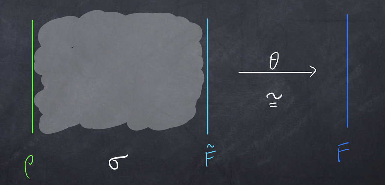
Figure 1. The sandwich picture of $(\sigma,\rho)$ acting on $F$: the $(\sigma,\rho)$-module structure on $F$

Our starting point here is an old idea: the separation of an abstract symmetry structure from a concrete realization as symmetries of some object. The advent of abstract groups [W] was a significant development in mathematics, as was the advent of abstract algebras. We offer an abstract symmetry structure in the context of field theory as Definition 3.1 and its concrete realization on a field theory as Definition 3.2. For broad conceptual purposes one can analogize a field theory to a linear representation of a Lie group or to a module over an algebra, and these analogies inspire some of our nomenclature, for example the use of module for a boundary theory. The essential content of our definition is that the action of a “symmetry algebra” on an $n$-dimensional field theory $F$ expresses $F$ as a sandwich $\rho\otimes_{\sigma}\widetilde{F}$ in which $\sigma$ is an $(n+1)$-dimensional topological field theory; $\rho$ is a topological right boundary theory of $\sigma$, often assumed to be regular or Dirichlet; and $\widetilde{F}$ is a left boundary theory of $\sigma$, which typically is not topological. The sandwich—the dimensional reduction of $\sigma$ on an interval with endpoints colored by $\rho$ and $\widetilde{F}$—together with an isomorphism $\theta$ to the original theory $F$, is depicted in Figure 1. Defects supported away from $\widetilde{F}$-boundaries belong to the topological theory $\sigma$ with its topological right boundary theory $\rho$, the pair $(\sigma,\rho)$ that comprises the abstract symmetry structure. We introduce the term $n$-dimensional quiche for the pair $(\sigma,\rho)$. These topological defects act in the quantum field theory $F$ by transport via the isomorphism $\theta$, but they can be manipulated universally in the topological field theory $(\sigma,\rho)$ independently of any particular $(\sigma,\rho)$-module. In this sense $(\sigma,\rho)$-defects are analogous to elements of an abstract algebra. This also provides a connection to the work of [GKSW].

Another aspect of our work is a clarification of the role of topological defects and their relation to symmetries. In §2 we give a definition of local and global topological defects, together with a description of background fields in the presence of these defects. We also construct a composition law on topological defects. We stress that the composition law preserves the codimension of defects: the composition of two codimension $\ell$ defects is a codimension $\ell$ defect, notwithstanding claims one often hears to the contrary.

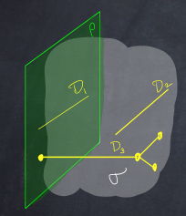
Figure 2. The quiche $(\sigma,\rho)$, a $\rho$-defect $D_{1}$ (on the boundary), and $(\sigma,\rho)$-defects $D_{2}$ (in the bulk) and $D_{3}$ (emanating from the boundary)

The sandwich presentation of a theory with symmetry appears in earlier talks and papers, such as [Te, GKSW, FT1, GK]; see also [FFRS] and the references therein for early links between defects and symmetry. However, the use of the sandwich presentation to develop a calculus of topological defects acting on a quantum field theory—and to do so based on fully local topological field theory—is new. (Theories of defects in topological field theory are not new: [FFRS, KaSa, FSV] is a small sample of older literature.)

Topological field theory imposes strong finiteness constraints, called dualizability, but one can relax those constraints as follows. In the lingo, one takes  $\sigma$ to be a once-categorified $n$-dimensional topological field theory and takes $\rho$ and $\widetilde{F}$ to be a relative field theory to $\sigma$. We make comments in this direction throughout, though in almost all of our examples $\sigma$ is a full $(n+1)$-dimensional theory. Under the basic analogy of field theory with Lie group representations, $(\sigma,\rho)$-modules with $\sigma$ a full $(n+1)$-dimensional theory correspond to representations of finite groups. It is desirable to investigate in greater depth analogs of infinite discrete group and compact Lie group symmetries.

We begin in Section 1 with a quick exposition of groups and algebras of symmetries. The case of algebras (§1.2) provides the most direct motivation for our definitions. We discuss quotients and projective symmetries in these contexts; both have echos in field theory. In Section 2 we review formal ideas in Wick-rotated field theory. The basic framework sees a field theory as a linear representation of a geometric bordism category, an idea most developed for topological theories. We introduce domain walls, boundaries, and more general defects. Our treatment here is quite heuristic, favoring exposition over precision; a technically complete account is possible for topological theories. As already stated, our main definitions are in Section 3. We illustrate with a few examples in §3.3, deferring more details and more intricate examples to §4. Section 3 concludes with a general discussion of quotients by symmetries and finite electromagnetic duality, which realizes quotients for a special class of symmetries.

Section 4 illustrates our formulation of symmetry through a series of examples. The case of symmetries in quantum mechanics (§4.2), which we linger over, makes contact with the motivating scenario of modules over an algebra and also provides valuable intuition for higher dimensional theories. From there we move on to examples in higher dimensions and examples with higher symmetry. We focus on the composition law for defects, which often does not have a valid expression in classical terms. We conclude in Section 5 with a discussion of quotient defects, duality defects, and some applications thereof.

There is a class of topological field theories constructed by a finite version of the Feynman path integral. These finite homotopy theories are the subject of Appendix A. In the basic case one sums over maps into a $\pi$-finite space. (Significantly, one can drop $\pi$-finiteness and construct a once-categorified theory from any topological space.) These theories are a fertile laboratory for general concepts in field theory, and as well they are often the basis of a symmetry structure which acts on quantum field theories of interest. By their nature they are amenable to computations based on topological rather than analytic techniques. We sketch how to manipulate defects in such theories.

As already mentioned, our goal in this paper is to illustrate the sandwich formulation of symmetries and the resulting topological calculus of defects rather than to give a complete and rigorous development. We also remark that unitarity is not brought in here, but of course it is important for physical applications to do so. Our referencing is hardly complete; we refer the reader to the recent Snowmass whitepaper on generalized symmetries [CDIS] as well as the Snowmass whitepaper on physical mathematics [BFMNRS, §2.5] for more perspective, examples, and references. The lecture notes [F3] cover much of the same ground, but there are some different examples developed there as well. See also the conference proceedings [F4], which contains additional motivation and an application to line defects in 4-dimensional gauge theories.

We offer this work as a tribute to Vaughan Jones, whose untimely passing is a great loss, both mathematically and personally. We treasure the memories of our interactions with Vaughan in the realms of mathematics, physics, and well beyond.

Ibou Bah, David Ben-Zvi, Mike Freedman, Dan Friedan, Mike Hopkins, Theo Johnson-Freyd, Alexei Kitaev, Justin Kulp, Kiran Luecke, Ingo Runkel, Will Stewart, and Jingxiang Wu offered valuable comments, for which we thank them all. This research is under the auspices of the Simons Collaboration on Global Categorical Symmetry, and we thank our colleagues for their valuable feedback. We are grateful to Andrew Moore for his expert rendering of Figure 8.

1. Groups and algebras of symmetries

We review two settings for symmetry in mathematics: groups of symmetries  (§1.1) and algebras of symmetries (§1.2). (Appendix A generalizes the former in a topological setting.) In each instance we restrict our exposition for the most part to the simplest case of finite symmetries, though many considerations generalize beyond the finite case. In particular, the groups and algebras carry no topology. For each there is abstract “symmetry data” as well as concrete realizations of that symmetry data. The distinction between abstract symmetry and its concrete realizations serves us well when we come to field theory in §3. Here, in §1.3, we discuss quotients in both the group and algebra contexts. We conclude with brief discussions of projective symmetries (§1.4) and higher algebras of symmetries (§1.5).

1.1. Fibering over $BG$

Let $G$ be a finite group. A classifying space $BG$ is derived from a contractible topological space $EG$ equipped with a free $G$-action by taking the quotient; the homotopy type of $BG$ is independent of choices. If $X$ is a topological space equipped with a $G$-action, then the Borel construction is the total space of a fiber bundle

(1.1) $$\begin{gathered}\lx@xy@svg{\hbox{\raise 0.0pt\hbox{\kern 10.97464pt\hbox{\ignorespaces\ignorespaces\ignorespaces\hbox{\vtop{\kern 0.0pt\offinterlineskip\halign{\entry@#!@&&\entry@@#!@\cr&\\\crcr}}}\ignorespaces{\hbox{\kern-9.7362pt\raise 0.0pt\hbox{\hbox{\kern 0.0pt\raise 0.0pt\hbox{\hbox{\kern 3.0pt\raise 0.0pt\hbox{$\textstyle{X_{G}\ignorespaces\ignorespaces\ignorespaces\ignorespaces}$}}}}}}}\ignorespaces\ignorespaces\ignorespaces\ignorespaces{}{\hbox{\lx@xy@droprule}}\ignorespaces\ignorespaces\ignorespaces{\hbox{\kern 0.0pt\raise-19.12332pt\hbox{{}\hbox{\kern 0.0pt\raise 0.0pt\hbox{\hbox{\kern 3.0pt\hbox{\hbox{\kern 0.0pt\raise-1.50694pt\hbox{$\scriptstyle{\pi}$}}}\kern 3.0pt}}}}}}\ignorespaces{\hbox{\kern 0.0pt\raise-28.41333pt\hbox{\hbox{\kern 0.0pt\raise 0.0pt\hbox{\lx@xy@tip{1}\lx@xy@tip{-1}}}}}}{\hbox{\lx@xy@droprule}}{\hbox{\lx@xy@droprule}}{\hbox{\kern 6.97464pt\raise 0.0pt\hbox{\hbox{\kern 0.0pt\raise 0.0pt\hbox{\hbox{\kern 3.0pt\raise 0.0pt\hbox{$\textstyle{=EG\times^{\vphantom{1*\prime y\vee M}}_{G}X}$}}}}}}}{\hbox{\kern-10.97464pt\raise-38.24664pt\hbox{\hbox{\kern 0.0pt\raise 0.0pt\hbox{\hbox{\kern 3.0pt\raise 0.0pt\hbox{$\textstyle{BG}$}}}}}}}\ignorespaces}}}}\ignorespaces\end{gathered} \textstyle{X_{G}\ignorespaces\ignorespaces\ignorespaces\ignorespaces} \scriptstyle{\pi} \textstyle{=EG\times^{\vphantom{1*\prime y\vee M}}_{G}X} \textstyle{BG} \textstyle{X_{G}\ignorespaces\ignorespaces\ignorespaces\ignorespaces} \scriptstyle{\pi} \textstyle{=EG\times^{\vphantom{1*\prime y\vee M}}_{G}X} \textstyle{BG}$$

with fiber $X$. If $*\in BG$ is a chosen point, and we choose a basepoint in the $G$-orbit in $EG$ labeled by $*$, then the fiber $\pi^{-1}(*)$ is canonically identified with $X$. We say the abstract (group) symmetry data is the pair $(BG,*)$, and a realization of the symmetry $(BG,*)$ on $X$ is a fiber bundle (1.1) over $BG$ together with an identification of the fiber over $*\in BG$ with $X$.

Remark .

We use a pair $(\mathscr{X},*)$ consisting of a $\pi$-finite topological space $\mathscr{X}$ and a basepoint $*\in\mathscr{X}$ as a generalization of $(BG,*)$. In this context the based loop space $\Omega\mathscr{X}$ is a higher, homotopical version of a finite group: a grouplike $A_{\infty}$-space [Sta], which is the generalization of the more classical $H$-group [Sp, §1.5] that takes into account higher coherence. For simplicity we call these higher finite groups.

1.2. Algebras of symmetries

Let $A$ be an algebra, and for simplicity suppose that the ground field is ${\mathbb{C}}$. For our expository purposes it suffices to assume that $A$ and the modules that follow are finite dimensional. Let $R$ be the right regular $A$-module, i.e., the vector space $A$ furnished with the right action of $A$ by multiplication. The pair $(A,R)$ is abstract (algebra) symmetry data: the action of $(A,R)$ on a vector space $V$ is a pair $(L,\theta)$ consisting of a left $A$-module $L$ together with an isomorphism of vector spaces

(1.2) $$\theta\colon R\,\otimes^{\vphantom{1*\prime y\vee M}}_{A}L\xrightarrow{\;\;\cong\;\;}V.$$

Example .

Let $G$ be a finite group. The group algebra $A={\mathbb{C}}[G]$ is the free vector space on the set $G$, which is then a linear basis of $A$; multiply basis elements according to the group law in $G$. A left $A$-module $L$ is canonically identified as a linear representation of $G$. The tensor product in (1.2) recovers the vector space which underlies the representation. In the setup of §1.1, take $X=L$ to construct a vector bundle $L_{G}\to BG$ whose fiber over $*\in BG$ is $L$.

Observe that the right regular module satisfies the algebra isomorphism

(1.3) $$\operatorname{End}_{A}(R)\cong A,$$

where the left hand side is the algebra of linear maps $R\to R$ that commute with the right $A$-action.

1.3. Quotients

In the topological setting of §1.1, the total space $X_{G}$ of the Borel construction plays the role of the quotient space $X/G$. Indeed, if $G$ acts freely on $X$, then there is a homotopy equivalence $X_{G}\simeq X/G$; in general, $X_{G}$ is the homotopy quotient.

For any map $f\colon Y\to BG$ of topological spaces we form the homotopy pullback

(1.4) $$\begin{gathered}\lx@xy@svg{\hbox{\raise 0.0pt\hbox{\kern 7.01389pt\hbox{\ignorespaces\ignorespaces\ignorespaces\hbox{\vtop{\kern 0.0pt\offinterlineskip\halign{\entry@#!@&&\entry@@#!@\cr&\\&&\\&\crcr}}}\ignorespaces{\hbox{\kern-3.0pt\raise 0.0pt\hbox{\hbox{\kern 0.0pt\raise 0.0pt\hbox{\hbox{\kern 3.0pt\raise 0.0pt\hbox{$\textstyle{}$}}}}}}}{\hbox{\kern 35.2177pt\raise 0.0pt\hbox{\hbox{\kern 0.0pt\raise 0.0pt\hbox{\hbox{\kern 3.0pt\raise 0.0pt\hbox{$\textstyle{Z\ignorespaces\ignorespaces\ignorespaces\ignorespaces\ignorespaces\ignorespaces\ignorespaces\ignorespaces}$}}}}}}}\ignorespaces\ignorespaces\ignorespaces{}\ignorespaces\ignorespaces{\hbox{\lx@xy@drawline@}}\ignorespaces{\hbox{\kern 7.0139pt\raise-31.47473pt\hbox{\hbox{\kern 0.0pt\raise 0.0pt\hbox{\lx@xy@tip{1}\lx@xy@tip{-1}}}}}}\ignorespaces\ignorespaces{\hbox{\lx@xy@drawline@}}\ignorespaces{\hbox{\lx@xy@drawline@}}\ignorespaces\ignorespaces\ignorespaces{}\ignorespaces\ignorespaces{\hbox{\lx@xy@drawline@}}\ignorespaces{\hbox{\kern 76.96317pt\raise-29.57506pt\hbox{\hbox{\kern 0.0pt\raise 0.0pt\hbox{\lx@xy@tip{1}\lx@xy@tip{-1}}}}}}\ignorespaces\ignorespaces{\hbox{\lx@xy@drawline@}}\ignorespaces{\hbox{\lx@xy@drawline@}}{\hbox{\kern-7.01389pt\raise-37.78998pt\hbox{\hbox{\kern 0.0pt\raise 0.0pt\hbox{\hbox{\kern 3.0pt\raise 0.0pt\hbox{$\textstyle{Y\ignorespaces\ignorespaces\ignorespaces\ignorespaces}$}}}}}}}\ignorespaces\ignorespaces\ignorespaces{}\ignorespaces\ignorespaces{\hbox{\lx@xy@drawline@}}\ignorespaces\ignorespaces\ignorespaces{\hbox{\kern 11.32074pt\raise-62.79607pt\hbox{{}\hbox{\kern 0.0pt\raise 0.0pt\hbox{\hbox{\kern 3.0pt\hbox{\hbox{\kern 0.0pt\raise-1.75pt\hbox{$\scriptstyle{f}$}}}\kern 3.0pt}}}}}}\ignorespaces{\hbox{\kern 31.0701pt\raise-65.74664pt\hbox{\hbox{\kern 0.0pt\raise 0.0pt\hbox{\lx@xy@tip{1}\lx@xy@tip{-1}}}}}}\ignorespaces\ignorespaces{\hbox{\lx@xy@drawline@}}\ignorespaces{\hbox{\lx@xy@drawline@}}{\hbox{\kern 38.98853pt\raise-37.78998pt\hbox{\hbox{\kern 0.0pt\raise 0.0pt\hbox{\hbox{\kern 3.0pt\raise 0.0pt\hbox{$\textstyle{}$}}}}}}}{\hbox{\kern 76.96317pt\raise-37.78998pt\hbox{\hbox{\kern 0.0pt\raise 0.0pt\hbox{\hbox{\kern 3.0pt\raise 0.0pt\hbox{$\textstyle{X_{G}\ignorespaces\ignorespaces\ignorespaces\ignorespaces}$}}}}}}}\ignorespaces\ignorespaces\ignorespaces{}\ignorespaces\ignorespaces{\hbox{\lx@xy@drawline@}}\ignorespaces\ignorespaces\ignorespaces{\hbox{\kern 63.56348pt\raise-61.19191pt\hbox{{}\hbox{\kern 0.0pt\raise 0.0pt\hbox{\hbox{\kern 3.0pt\hbox{\hbox{\kern 0.0pt\raise-1.50694pt\hbox{$\scriptstyle{\pi}$}}}\kern 3.0pt}}}}}}\ignorespaces{\hbox{\kern 52.96318pt\raise-66.30939pt\hbox{\hbox{\kern 0.0pt\raise 0.0pt\hbox{\lx@xy@tip{1}\lx@xy@tip{-1}}}}}}\ignorespaces\ignorespaces{\hbox{\lx@xy@drawline@}}\ignorespaces{\hbox{\lx@xy@drawline@}}{\hbox{\kern-3.0pt\raise-75.57996pt\hbox{\hbox{\kern 0.0pt\raise 0.0pt\hbox{\hbox{\kern 3.0pt\raise 0.0pt\hbox{$\textstyle{}$}}}}}}}{\hbox{\kern 31.01389pt\raise-75.57996pt\hbox{\hbox{\kern 0.0pt\raise 0.0pt\hbox{\hbox{\kern 3.0pt\raise 0.0pt\hbox{$\textstyle{BG}$}}}}}}}\ignorespaces}}}}\ignorespaces\end{gathered} \textstyle{Z\ignorespaces\ignorespaces\ignorespaces\ignorespaces\ignorespaces\ignorespaces\ignorespaces\ignorespaces} \textstyle{Y\ignorespaces\ignorespaces\ignorespaces\ignorespaces} \scriptstyle{f} \textstyle{X_{G}\ignorespaces\ignorespaces\ignorespaces\ignorespaces} \scriptstyle{\pi} \textstyle{BG} \textstyle{Z\ignorespaces\ignorespaces\ignorespaces\ignorespaces\ignorespaces\ignorespaces\ignorespaces\ignorespaces} \textstyle{Y\ignorespaces\ignorespaces\ignorespaces\ignorespaces} \scriptstyle{f} \textstyle{X_{G}\ignorespaces\ignorespaces\ignorespaces\ignorespaces} \scriptstyle{\pi} \textstyle{BG}$$

If $Y$ is path connected and pointed, then there is a homotopy equivalence $Y\simeq B(\Omega Y)$. If $BG$ also has a basepoint, and if the map $f\colon Y\to BG$ is basepoint-preserving, then $f$  is the classifying map of a homomorphism $\Omega Y\to G=\Omega BG$, at least in the $A_{\infty}$-homotopical sense. In this case $Z$ is the homotopy quotient of $X$ by the action of $\Omega Y$. As a special case, if $G^{\prime}\subset G$ is a subgroup, and $Y=BG^{\prime}\to BG$ is the classifying map of the inclusion, then $Z$ is homotopy equivalent to the total space of the Borel construction $X_{G^{\prime}}$. Hence (1.4) is a generalized quotient construction. For $G^{\prime}=\{e\}$ we have $Y=*$ and we recover $Z=X$, as in §1.1.

There is an analogous story in the setting §1.2 of algebras. An augmentation of an algebra $A$ is an algebra homomorphism $\epsilon\colon A\to{\mathbb{C}}$. Use $\epsilon$ to endow the scalars ${\mathbb{C}}$ with a right $A$-module structure: set $\lambda\cdot a=\lambda\epsilon(a)$ for $\lambda\in{\mathbb{C}}$, $a\in A$. If $L$ is a left $A$-module, the vector space

(1.5) $$Q={\mathbb{C}}\otimes^{\vphantom{1*\prime y\vee M}}_{A}L={\mathbb{C}}\otimes^{\vphantom{1*\prime y\vee M}}_{\epsilon}L$$

plays the role of the “quotient” of $L$ by $A$.

Example .

For the group algebra of a finite group $G$, there is a natural augmentation

(1.6) $$\epsilon\colon{\mathbb{C}}[G] \longrightarrow{\mathbb{C}}$$

$$\sum\limits_{g\in G}\lambda_{g}g \longmapsto\sum\limits_{g\in G}\lambda_{g}$$

where $\lambda_{g}\in{\mathbb{C}}$. If $L$ is a representation of $G$, extended to a left ${\mathbb{C}}[G]$-module, then the tensor product (1.5) is the vector space of coinvariants:

(1.7) $$1\otimes\ell=1\otimes g\cdot\ell,\qquad\ell\in L,\quad g\in G,$$

in the tensor product with the augmentation. More generally, an augmentation of ${\mathbb{C}}[G]$ is induced from a character of $G$, i.e., a 1-dimensional linear representation of $G$.

As a particular case, let $S$ be a finite set equipped with a left $G$-action, and let $L={\mathbb{C}}\langle S\rangle$ be the free vector space generated by $S$. Then for the natural augmentation (1.6), the vector space ${\mathbb{C}}\otimes^{\vphantom{1*\prime y\vee M}}_{\epsilon}L$ can be identified with ${\mathbb{C}}\langle S/G\rangle$, the free vector space on the quotient set. An arbitrary character $\chi\colon G\to{\mathbb{C}}^{\times}$ induces a line bundle $L_{\chi}\to S/\!/G$ over the groupoid or stack quotient, and for the associated augmentation $\epsilon\colon{\mathbb{C}}[G]\to{\mathbb{C}}$ the coinvariants $C\otimes_{\epsilon}L$ are isomorphic to the space of its global sections.

We can form the “sandwich” (1.5) with any right $A$-module in place of the augmentation. For $A={\mathbb{C}}[G]$, if $G^{\prime}\subset G$ is a subgroup, then ${\mathbb{C}}\langle G^{\prime}\backslash G\rangle$ is a right $G$-module; for $G^{\prime}=G$ it reduces to the augmentation module (1.6). If $L$ is a $G$-representation, then

(1.8) $${\mathbb{C}}\langle G^{\prime}\backslash G\rangle\otimes^{\vphantom{1*\prime y\vee M}}_{{\mathbb{C}}[G]}L\cong{\mathbb{C}}\otimes^{\vphantom{1*\prime y\vee M}}_{{\mathbb{C}}[G^{\prime}]}L$$

is the vector space of coinvariants of the restricted $G^{\prime}$-representation.

Remark .

There is a mismatch in our description of quotients in topology and quotients in algebra. To align our accounts, one should use derived quotients in algebra, and so replace the tensor product in (1.8) with the (left) derived tensor product, i.e., with Tor. Then one computes the entire complex homology of the Borel quotient, not just the free vector space generated by its components. However, this mismatch does not occur for finite groups in characteristic zero.

1.4. Projective symmetries

We begin with an example in the algebra framework §1.2. Let $G$ be a finite group, and suppose

(1.9) $$1\longrightarrow{\mathbb{C}}^{\times}\longrightarrow G^{\tau}\longrightarrow G\longrightarrow 1$$

is a central extension. Let $L^{\tau}\to G$ be the complex line bundle associated to the principal ${\mathbb{C}}^{\times}$-bundle (1.9). Define the twisted group algebra

(1.10) $$A^{\tau}=\bigoplus\limits_{g\in G}L^{\tau}_{g}.$$

Then $A^{\tau}$ inherits an algebra structure from the group structure of $G$. Furthermore, $G^{\tau}\subset A^{\tau}$ lies in the group of units. An $A^{\tau}$-module restricts to a linear representation of $G^{\tau}$ on which the center ${\mathbb{C}}^{\times}$ acts by scalar multiplication, and vice versa. Observe that there is no analog of the augmentation (1.6) unless the central extension (1.9) splits; indeed, an augmentation induces a splitting. (Restrict $A^{\tau}\to{\mathbb{C}}$ to $G^{\tau}\subset A^{\tau}$.) More generally, if $G^{\prime}\subset G$ is a subgroup, then a splitting of the restriction of (1.9) over $G^{\prime}$ induces an $A^{\tau}$-module structure on ${\mathbb{C}}\langle G^{\prime}\backslash G\rangle$, and we can use this to define the quotient by $G^{\prime}$, as in (1.8). Absent the splitting, the projectivity obstructs the quotient construction. There is an analogous story in the context of §1.1; see Remark A.3.2.

Remark .

That central extensions obstruct augmentations has an echo in field theory: ’t Hooft anomalies obstruct the quotient operation (gauging) by a symmetry.

1.5. Higher algebra

The higher versions of finite groups in Remark 1.1 have an analog in algebras as well. For example, a fusion category $\mathscr{A}$ is a “once higher” version of a finite dimensional semisimple algebra, and there is a well-developed theory of modules over a fusion category [EGNO]. In particular, $\mathscr{A}$ is a right module over itself, the right regular module. A finite group $G$ gives rise to the fusion category $\mathscr{A}=\operatorname{Vect}[G]$ of finite rank vector bundles over $G$ with convolution product. The analog of an augmentation for a fusion category $\mathscr{A}$ is a fiber functor—a tensor functor $\mathscr{A}\to\operatorname{Vect}$—and for $\mathscr{A}=\operatorname{Vect}[G]$ the natural choice is pushforward under the map $G\to*$ to a point. More generally, by analogy with characters as augmentations of ${\mathbb{C}}[G]$, a central extension of $G$ by ${\mathbb{C}}^{\times}$ produces a fiber functor $\operatorname{Vect}[G]\to\operatorname{Vect}$. If $\omega$ is a cocycle which represents an element of $H^{3}(G;{\mathbb{C}}^{\times})$, then there is a twisted variant $\operatorname{Vect}^{\omega}[G]$, but there is no fiber functor if the cohomology class of $\omega$ is nonzero; see Figure 34.

Higher categorical generalizations of fusion categories are a topic of much current interest and development, and presumably have analogs of the constructions presented above.

2. Formal structures in field theory

We review basic notions in Wick-rotated field theory on compact manifolds. Segal [S1] initiated this framework for 2-dimensional conformal field theories. Recently, Kontsevich-Segal [KS] discuss general quantum field theories from this viewpoint. The entire story is most developed for topological field theories, beginning with Atiyah [A], who made the connection to Thom’s theory of bordism; continuing with the introduction and development of fully local field theory [F1, La, BD, L]; and then with the connection of fully local field theory to defects [K]. (We have only skimmed the surface of relevant literature.) Our exposition emphasizes the metaphor:

(2.1) field theory $$\sim$$ representation of a Lie group

We briefly touch on axioms (§2.1), domain walls (§2.2), boundary theories and anomalies (§2.3), and general defects (§2.4). There is no pretense of rigor or completeness here. For the topological case there are rigorous definitions in the literature for most of what we write; a few items are still under development.

2.1. Axioms

The discrete parameters that determine the “type” of field theory are a nonnegative integer $n$ and a collection $\mathcal{F}$ of $n$-dimensional fields. One thinks of $n$ as the dimension of spacetime and $\mathcal{F}$ as the collection of background fields. Some fields have a topological flavor—orientations, spin structures, etc.—while others are more geometric—Riemannian metrics, connections for a fixed gauge group, scalar fields, spinor fields, etc. (There are no fluctuating fields; they have already been “integrated out” before the formulation in this axiom system. Nor is there spacetime; we work in the Wick-rotated setting in which every nonzero tangent vector is spacelike.) There is a bordism category $\operatorname{Bord}_{n}(\mathcal{F})$ of $n$-dimensional smooth manifolds $M$ with corners equipped with a choice of fields, i.e., an object in $\mathcal{F}(M)$. We refer to the literature for more details, say [L, CS] for the fully local topological case and [KS] for the nonextended general case. We assume that all topological theories are fully local (i.e., fully extended downward in dimension), in which case $\operatorname{Bord}_{n}(\mathcal{F})$ is a symmetric monoidal $n$-category. In the nonextended case, we interpret ‘$\operatorname{Bord}_{n}(\mathcal{F})$’ as a 1-category $\operatorname{Bord}_{\langle n-1,n\rangle}(\mathcal{F})$ whose objects are closed $(n-1)$-manifolds and whose morphisms are bordisms between them. Let $\mathscr{C}$ be a symmetric monoidal $n$-category. A topological field theory is a symmetric monoidal functor

(2.2) $$F\colon\operatorname{Bord}_{n}(\mathcal{F})\longrightarrow\mathscr{C}.$$

Recall that the cobordism hypothesis [L] enables a calculus of such functors in terms of duality data inside the codomain category $\mathscr{C}$. Turning to nontopological theories, a similar calculus is not in place and is a subject of wide interest. In the meantime, we confine ourselves to nonextended nontopological theories, and so replace $\mathscr{C}$ by the 1-category $t\!\operatorname{Vect}$ of suitable complex topological vector spaces under tensor product. Finally, a field theory may be evaluated in smooth families parametrized by a smooth manifold $S$, and it should behave well under base change. Therefore, (2.2) should be sheafified over $\operatorname{Man}$, the site of smooth manifolds and smooth diffeomorphisms [ST]. This applies to both topological and nontopological field theories.

Remark .

1. A topological field theory imposes strong finiteness. In the metaphor (2.1), a topological field theory is analogous to a representation of a finite group. We also use the notion of a once-categorified $n$-dimensional field theory, which in the topological case is a symmetric monoidal functor $\operatorname{Bord}_{n}(\mathcal{F})\to\mathscr{C}$, where $\mathscr{C}$ is a symmetric monoidal $(n+1)$-category. With typical choices of codomain $\mathscr{C}$, in the top dimension such a theory assigns a vector space rather than a complex number. The finiteness conditions are more relaxed than in a full topological field theory; for example, the vector spaces attached to top dimensional closed manifolds need not be finite dimensional in a once-categorified topological theory.

2. The collection of field theories of a fixed dimension $n$ on a fixed collection $\mathcal{F}$ of background fields has an associative composition law: juxtaposition of quantum systems with no interaction, sometimes called ‘stacking’. We denote this composition law as a tensor product. For example, on a closed $(n-1)$-manifold $Y$ the state space $(F_{1}\otimes F_{2})(Y)$ is the tensor product $F_{1}(Y)\otimes F_{2}(Y)$ of the state spaces of the constituent systems. There is a unit theory $\mathbbm{1}$ for this operation. For example, if $F_{1},F_{2}$ are theories, and $Y$ is a closed $(n-1)$-manifold with background fields, then $(F_{1}\otimes F_{2})(Y)=F_{1}(Y)\otimes F_{2}(Y)$. The unit theory has $\mathbbm{1}(Y)={\mathbb{C}}$; there is a single state on every space. There is then a subcategory of units for the composition law: invertible field theories.

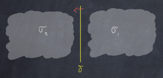
Figure 3. A domain wall $\delta\colon\sigma_{1}\to\sigma_{2}$

2.2. Domain walls

Let $\sigma_{1},\sigma_{2}$ be $(n+1)$-dimensional theories on background fields $\mathcal{F}_{1},\mathcal{F}_{2}$ with common codomain $\mathscr{C}$. (Recall the notation for background fields in footnote ⁷. In the sequel ‘$\sigma$’ usually denotes a topological field theory, but in this section the theories $\sigma_{i}$ need not be topological.) A domain wall $\delta\colon\sigma_{1}\to\sigma_{2}$ is the analog of a bimodule, so we use the convenient terminology ‘$(\sigma_{2},\sigma_{1})$-bimodule’; see Figure 3 for a depiction. In the topological case one can build a higher category in which a domain wall is a 1-morphism, but we do not pursue that here. The triple $(\sigma_{1},\sigma_{2},\delta)$ is formally a functor with domain a bordism category of smooth $(n+1)$-dimensional manifolds with corners, each equipped with a partition into regions labeled ‘1’ and ‘2’ separated by a cooriented codimension one submanifold (with corners) which is “$\delta$-colored”; the codomain of the functor is $\mathscr{C}$. The bordism category is illustrated in Figure 4 in the top dimension. See [L, Example 4.3.23] for the topological case, though of course the notion transcends the purely topological. The background fields $\mathcal{F}\colon\operatorname{Man}_{n+1}^{\textnormal{op}}\to\operatorname{Set}_{\Delta}$ on the domain wall form a correspondence

(2.3) $$\begin{gathered}\lx@xy@svg{\hbox{\raise 0.0pt\hbox{\kern 7.6639pt\hbox{\ignorespaces\ignorespaces\ignorespaces\hbox{\vtop{\kern 0.0pt\offinterlineskip\halign{\entry@#!@&&\entry@@#!@\cr&\\&&\crcr}}}\ignorespaces{\hbox{\kern-3.0pt\raise 0.0pt\hbox{\hbox{\kern 0.0pt\raise 0.0pt\hbox{\hbox{\kern 3.0pt\raise 0.0pt\hbox{$\textstyle{}$}}}}}}}{\hbox{\kern 31.6639pt\raise 0.0pt\hbox{\hbox{\kern 0.0pt\raise 0.0pt\hbox{\hbox{\kern 3.0pt\raise 0.0pt\hbox{$\textstyle{\mathcal{F}\ignorespaces\ignorespaces\ignorespaces\ignorespaces\ignorespaces\ignorespaces\ignorespaces\ignorespaces}$}}}}}}}\ignorespaces\ignorespaces\ignorespaces{}\ignorespaces\ignorespaces{\hbox{\lx@xy@drawline@}}\ignorespaces{\hbox{\kern 7.66391pt\raise-30.10905pt\hbox{\hbox{\kern 0.0pt\raise 0.0pt\hbox{\lx@xy@tip{1}\lx@xy@tip{-1}}}}}}\ignorespaces\ignorespaces{\hbox{\lx@xy@drawline@}}\ignorespaces{\hbox{\lx@xy@drawline@}}\ignorespaces\ignorespaces\ignorespaces{}\ignorespaces\ignorespaces{\hbox{\lx@xy@drawline@}}\ignorespaces{\hbox{\kern 68.1917pt\raise-30.11655pt\hbox{\hbox{\kern 0.0pt\raise 0.0pt\hbox{\lx@xy@tip{1}\lx@xy@tip{-1}}}}}}\ignorespaces\ignorespaces{\hbox{\lx@xy@drawline@}}\ignorespaces{\hbox{\lx@xy@drawline@}}{\hbox{\kern-7.6639pt\raise-37.73553pt\hbox{\hbox{\kern 0.0pt\raise 0.0pt\hbox{\hbox{\kern 3.0pt\raise 0.0pt\hbox{$\textstyle{\mathcal{F}_{1}}$}}}}}}}{\hbox{\kern 34.9278pt\raise-37.73553pt\hbox{\hbox{\kern 0.0pt\raise 0.0pt\hbox{\hbox{\kern 3.0pt\raise 0.0pt\hbox{$\textstyle{}$}}}}}}}{\hbox{\kern 68.1917pt\raise-37.73553pt\hbox{\hbox{\kern 0.0pt\raise 0.0pt\hbox{\hbox{\kern 3.0pt\raise 0.0pt\hbox{$\textstyle{\mathcal{F}_{2}}$}}}}}}}\ignorespaces}}}}\ignorespaces\end{gathered} \textstyle{\mathcal{F}\ignorespaces\ignorespaces\ignorespaces\ignorespaces\ignorespaces\ignorespaces\ignorespaces\ignorespaces} \textstyle{\mathcal{F}_{1}} \textstyle{\mathcal{F}_{2}} \textstyle{\mathcal{F}\ignorespaces\ignorespaces\ignorespaces\ignorespaces\ignorespaces\ignorespaces\ignorespaces\ignorespaces} \textstyle{\mathcal{F}_{1}} \textstyle{\mathcal{F}_{2}}$$

Thus we can have geometric domain walls which depend on a Riemannian metric between topological theories, or in the purely topological case a spin domain wall between oriented theories, etc. As a special case, a domain wall from the tensor unit theory $\mathbbm{1}$ to itself is an $n$-dimensional (absolute, standalone) theory, though with $(n+1)$-dimensional fields instead of $n$-dimensional fields. More generally, we can tensor any domain wall $\delta\colon\sigma_{1}\to\sigma_{2}$ with an $n$-dimensional theory to obtain a new domain wall.

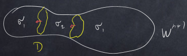
Figure 4. Domain walls in the manifold $W$

There is a composition law on topological domain walls:

(2.4) $$\begin{gathered}\lx@xy@svg{\hbox{\raise 0.0pt\hbox{\kern 7.25706pt\hbox{\ignorespaces\ignorespaces\ignorespaces\hbox{\vtop{\kern 0.0pt\offinterlineskip\halign{\entry@#!@&&\entry@@#!@\cr&&\crcr}}}\ignorespaces{\hbox{\kern-7.25706pt\raise 0.0pt\hbox{\hbox{\kern 0.0pt\raise 0.0pt\hbox{\hbox{\kern 3.0pt\raise 0.0pt\hbox{$\textstyle{\sigma_{1}\ignorespaces\ignorespaces\ignorespaces\ignorespaces\ignorespaces\ignorespaces\ignorespaces\ignorespaces\ignorespaces}$}}}}}}}\ignorespaces\ignorespaces\ignorespaces\ignorespaces{}{\hbox{\lx@xy@droprule}}\ignorespaces\ignorespaces\ignorespaces{\hbox{\kern 14.15152pt\raise 5.98611pt\hbox{{}\hbox{\kern 0.0pt\raise 0.0pt\hbox{\hbox{\kern 3.0pt\hbox{\hbox{\kern 0.0pt\raise-2.98611pt\hbox{$\scriptstyle{\delta^{\prime}}$}}}\kern 3.0pt}}}}}}\ignorespaces{\hbox{\kern 31.25706pt\raise 0.0pt\hbox{\hbox{\kern 0.0pt\raise 0.0pt\hbox{\lx@xy@tip{1}\lx@xy@tip{-1}}}}}}{\hbox{\lx@xy@droprule}}{\hbox{\lx@xy@droprule}}\ignorespaces\ignorespaces\ignorespaces\ignorespaces\ignorespaces{}{}{}{{}{}{}{}{}{}{}{}{}{}{}{}{}{}}{}\ignorespaces\hbox{\hbox{\kern 0.0pt\raise 0.0pt\hbox{{}{}{{}}{{}{}{}}{}}}}\ignorespaces{}\ignorespaces{}{}{}{{}{}}\ignorespaces\ignorespaces{\hbox{\kern 28.16974pt\raise-17.9861pt\hbox{{}\hbox{\kern 0.0pt\raise 0.0pt\hbox{\hbox{\kern 3.0pt\hbox{\hbox{\kern 0.0pt\raise-2.98611pt\hbox{$\scriptstyle{\delta^{\prime\prime}\circ\,\delta^{\prime}}$}}}\kern 3.0pt}}}}}}\ignorespaces{}{}{}{{}{}{}{}{}{}{}{}{}{}{}{}{}{}{}{}{}{}{}{}}{\hbox{\kern 69.76929pt\raise-4.09717pt\hbox{\hbox{\kern 0.0pt\raise 0.0pt\hbox{\lx@xy@tip{1}\lx@xy@tip{-1}}}}}}\ignorespaces\hbox{\hbox{\kern 0.0pt\raise 0.0pt\hbox{{}{}{}{{}}{{}{}{}\lx@xy@spline@}{}}}}\ignorespaces{}\ignorespaces\hbox{\hbox{\kern 0.0pt\raise 0.0pt\hbox{{}{}{{}}{{}{}{}}{}}}}\ignorespaces{}{\hbox{\kern 31.25706pt\raise 0.0pt\hbox{\hbox{\kern 0.0pt\raise 0.0pt\hbox{\hbox{\kern 3.0pt\raise 0.0pt\hbox{$\textstyle{\sigma_{2}\ignorespaces\ignorespaces\ignorespaces\ignorespaces}$}}}}}}}\ignorespaces\ignorespaces\ignorespaces\ignorespaces{}{\hbox{\lx@xy@droprule}}\ignorespaces\ignorespaces\ignorespaces{\hbox{\kern 52.11566pt\raise 5.98611pt\hbox{{}\hbox{\kern 0.0pt\raise 0.0pt\hbox{\hbox{\kern 3.0pt\hbox{\hbox{\kern 0.0pt\raise-2.98611pt\hbox{$\scriptstyle{\delta^{\prime\prime}}$}}}\kern 3.0pt}}}}}}\ignorespaces{\hbox{\kern 69.7712pt\raise 0.0pt\hbox{\hbox{\kern 0.0pt\raise 0.0pt\hbox{\lx@xy@tip{1}\lx@xy@tip{-1}}}}}}{\hbox{\lx@xy@droprule}}{\hbox{\lx@xy@droprule}}{\hbox{\kern 69.7712pt\raise 0.0pt\hbox{\hbox{\kern 0.0pt\raise 0.0pt\hbox{\hbox{\kern 3.0pt\raise 0.0pt\hbox{$\textstyle{\sigma_{3}}$}}}}}}}\ignorespaces}}}}\ignorespaces\end{gathered} \textstyle{\sigma_{1}\ignorespaces\ignorespaces\ignorespaces\ignorespaces\ignorespaces\ignorespaces\ignorespaces\ignorespaces\ignorespaces} \scriptstyle{\delta^{\prime}} \scriptstyle{\delta^{\prime\prime}\circ\,\delta^{\prime}} \textstyle{\sigma_{2}\ignorespaces\ignorespaces\ignorespaces\ignorespaces} \scriptstyle{\delta^{\prime\prime}} \textstyle{\sigma_{3}} \textstyle{\sigma_{1}\ignorespaces\ignorespaces\ignorespaces\ignorespaces\ignorespaces\ignorespaces\ignorespaces\ignorespaces\ignorespaces} \scriptstyle{\delta^{\prime}} \scriptstyle{\delta^{\prime\prime}\circ\,\delta^{\prime}} \textstyle{\sigma_{2}\ignorespaces\ignorespaces\ignorespaces\ignorespaces} \scriptstyle{\delta^{\prime\prime}} \textstyle{\sigma_{3}}$$

2.3. Boundary theories, anomalies, and anomalous theories

Following the metaphor of domain wall as bimodule, there are special cases of right or left modules. For field theory these are called right boundary theories or left boundary theories, as depicted in Figure 5. (Normally, we omit the region labeled by the tensor unit theory ‘$\mathbbm{1}$’ in the drawings.) A right boundary theory of $\sigma$ is a domain wall $\sigma\to\mathbbm{1}$; a left boundary theory is a domain wall $\mathbbm{1}\to\sigma$. The nomenclature of right vs. left may at first be confusing; it does follow standard usage for modules over an algebra—the direction (right or left) is that of the action of the algebra on the module. In fact, following our general usage for domain walls, we sometimes use the terms ‘right $\sigma$-module’ and ‘left $\sigma$-module’ for right and left boundary theories.

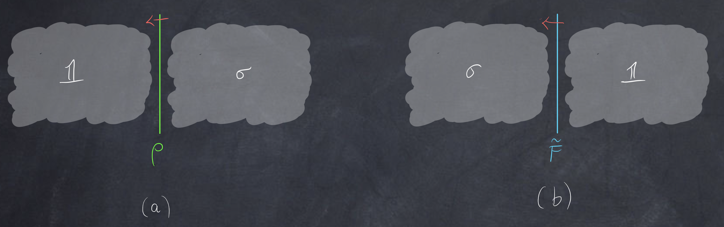
Figure 5. (a) a right boundary theory (b) a left boundary theory

A special nomenclature is used for the special case in which the bulk theory is invertible.

Definition .

Let $\alpha$ be an invertible $(n+1)$-dimensional field theory. An anomalous field theory $F$ with anomaly $\alpha$ is a left $\alpha$-module.

The choice of left vs. right is a convention we make. We emphasize that the background fields for $\alpha$ and $F$ may be different, as in (2.3). For example, a free spinor field theory $F$ in 3 dimensions is defined on spin Riemannian manifolds, whereas the associated anomaly theory $\alpha$ is topological: it is defined on a bordism category of spin manifolds. In other words, $\mathcal{F}_{F}=\{\textnormal{metric, spin structure}\}$ whereas $\mathcal{F}_{\alpha}=\{\textnormal{spin structure}\}$.

Remark .

1. In the metaphor (2.1) of field theory as Lie group representation, an anomalous field theory is a projective representation and the anomaly is the cocycle that measures the induced central extension of the Lie group.

2. An $(n+1)$-dimensional topological field theory with a topological boundary theory is defined as a functor out of a bordism category usually denoted $\operatorname{Bord}^{\partial}_{n+1}$; see [L, Example 4.3.22].

3. A boundary theory of a once-categorified $n$-dimensional theory (Remark 2.1(1)) is called a relative field theory; it is defined on a subcategory of $\operatorname{Bord}_{n+1}$ which drastically constrains the allowed $(n+1)$-manifolds [Ste]. One can replace the $(n+1)$-dimensional theories in §2.2 and §2.3 with once-categorified $n$-dimensional theories. Since finiteness conditions for once-categorified topological field theories are relaxed, this leads to wider applicability.

2.4. Defects

Domain walls and boundaries are special cases of the general notion of a defect in a field theory. Our discussion here is specifically for topological theories; with modification, some aspects apply more generally (see Remark 2.4 below). Defects are supported on submanifolds, or more generally on stratified subsets. Our goal in this section is to outline a calculus of fully local topological defects based on the cobordism hypothesis. Just as fully local topological field theories are generated by data associated to a point, so too can global defects be generated by purely local data. The nature of this local data depends on the codimension of the defect, as we spell out below.

Suppose $m$ is a positive integer, $\mathcal{F}$ is a collection of background fields, and

(2.5) $$\sigma\colon\operatorname{Bord}_{m}(\mathcal{F})\longrightarrow\mathscr{C}$$

is a topological field theory with values in a symmetric monoidal $m$-category $\mathscr{C}$. (In our application to quiche, $m=n+1$.) We describe defects of codimension $\ell$ in a $k$-dimensional manifold $M$, where $k\in\{1,\dots,m\}$, $\ell\in\{1,\dots,m\}$ and $\ell\leq k$. (There are also defects of codimension 0, but they require a separate treatment which we do not give here.) Let $Z\subset M$ be a submanifold of codimension $\ell$, and let $\nu\subset M$ be an open tubular neighborhood of $Z\subset M$; assume the closure $\bar{\nu}$ is the total space of a fiber bundle $\bar{\nu}\to Z$ with fiber the closed $\ell$-dimensional disk. The fiber over $p\in Z$ is denoted $\bar{\nu}_{p}$; its boundary $\partial\bar{\nu}_{p}$ is diffeomorphic to the $\ell$-dimensional sphere $S^{\ell-1}$. It is the link of $Z\subset M$ at $p$; see Figure 6. Caution: the depicted point $p\in Z$ is not an embedded point defect in $Z$, but rather it is the support of the local defect data.

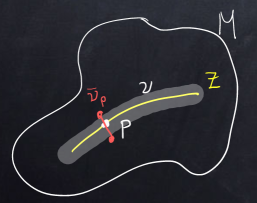
Figure 6. The tubular neighborhood and link of a submanifold

Remark .

Since $\sigma$ is a topological field theory, we may assume that the sheaf $\mathcal{F}$ is locally constant. In the presence of a defect supported on $Z$, the sheaf $\mathcal{F}\negmedspace\bigm{|}^{\vphantom{1*\prime y\vee M}}_{M}$ is refined to a constructible sheaf relative to the stratification $Z\subset M$. We elaborate in §2.5.

Definition .

Assume that $M$ is a closed manifold and $Z\subset M$ is a closed submanifold.

1. A local defect at $p\in Z$ is a morphism

   (2.6) $$\delta_{p}\in\operatorname{Hom}\bigl{(}1_{\Omega^{\ell-1}\mathscr{C}},\sigma(\partial\bar{\nu}_{p})\bigr{)}.$$

   Observe that $\sigma(\partial\bar{\nu}_{p})$ is an object in $\Omega^{\ell-1}\mathscr{C}$ (see footnote ⁸ for the definition of the loop category), $1_{\Omega^{\ell-1}\mathscr{C}}$ is the tensor unit object in $\Omega^{\ell-1}\mathscr{C}$, and $\delta_{p}$ is a 1-morphism in $\Omega^{\ell-1}\mathscr{C}$.

2. The transparent (local) defect is $\delta_{p}=\sigma(\bar{\nu}_{p})$, where we regard $\bar{\nu}_{p}$ as a bordism $\emptyset^{\ell-1}\to\partial\bar{\nu}_{p}$.

3. A global defect on $Z$ is a morphism

   (2.7) $$\delta_{Z}\in\operatorname{Hom}\bigl{(}1_{\Omega^{m-1}\mathscr{C}},\sigma(\partial\bar{\nu})\bigr{)};$$

   if $\Omega^{m-1}\mathscr{C}$ is a category of vector spaces, then $\delta_{Z}$  is a vector in a vector space.

4. The transparent (global) defect is $\delta_{Z}=\sigma(\bar{\nu})$.

The transparent defects can be erased safely.

We make several comments about this definition.

Remark .

$W=M\setminus\nu$ is a compact manifold with boundary $\partial\bar{\nu}$. Define the bordism $W\colon\partial\bar{\nu}\to\emptyset$ by letting the boundary be incoming. If $\delta_{Z}$ is a global defect, evaluate the theory on $(M,Z,\delta_{Z})$ as $\sigma(W)(\delta_{Z})$. This is of the same type as the value $\sigma(M)$ on the closed manifold $M$: a complex number if $\dim M=m$, a complex vector space if $\dim M=m-1$, etc.

Remark .

As written, Section 2.4 does not take into account background fields, a defect that we ameliorate in §2.5. The main idea is to replace the single datum in (2.6), (2.7) with a family of data parametrized by a space of background fields. For the local defect (2.6) it is the space $\mathcal{F}\Bigl{(}\operatorname{germ}\bigl{(}\{p\}\subset\nu_{p}\bigr{)}\Bigr{)}$, the value of the constructible sheaf $\mathcal{F}$ on the restriction of $Z\subset M$ to a neighborhood of $\{p\}\subset\nu_{p}$. For the global defect (2.7) it is the space $\mathcal{F}\bigl{(}\operatorname{germ}(\partial\bar{\nu})\bigr{)}$, the value of the sheaf $\mathcal{F}$ on a germ of a neighborhood of $\partial\bar{\nu}$ in $M$.

Remark .

Section 2.4(1) defines a local defect at the point $p$ in the particular submanifold $Z\subset M$. There is also the notion of a local defect theory; it is defined in §2.5 below.

Remark .

Local defects can be integrated to global defects. The general case is discussed in §2.5. As an illustration in a special case, suppose $Z\subset W$ is equipped with a normal framing. This identifies each link $\partial\bar{\nu}_{p}$, $p\in Z$, with the standard sphere $S^{\ell-1}$. In this situation it makes sense to assign a single local defect

(2.8) $$\delta\in\operatorname{Hom}\bigl{(}1_{\Omega^{\ell-1}\mathscr{C}},\sigma(S^{\ell-1})\bigr{)}$$

to $Z$. Now $\sigma(S^{\ell-1})\in\Omega^{\ell-1}\mathscr{C}$ defines an $(m-\ell+1)$-dimensional field theory $\sigma^{(\ell-1)}$—the dimensional reduction of $\sigma$ along $S^{\ell-1}$—and a local defect  $\delta$ determines a left boundary theory $\delta^{(\ell-1)}$ for $\sigma^{(\ell-1)}$, if we assume sufficient finiteness (dualizability). Note that the cobordism hypothesis with singularities [L, §4.3] is used to define the boundary theory $\delta^{(\ell-1)}$. In turn, that boundary theory is used to integrate the local defect (2.8) to the global defect

(2.9) $$\delta_{Z}=\bigl{(}\sigma^{(\ell-1)},\delta^{(\ell-1)}\bigr{)}\bigl{(}[0,1]\times Z\bigr{)}\;\in\operatorname{Hom}\bigl{(}1_{\Omega^{m-1}\mathscr{C}},\sigma(Z\times S^{\ell-1})\bigr{)},$$

where $\{0\}\times Z$ is colored with the boundary theory $\delta^{(\ell-1)}$ and $\{1\}\times Z$ is outgoing.

So far this we have not specified background fields. To begin that discussion, observe that the theory $\sigma^{(\ell-1)}$ takes values in $\Omega^{\ell-1}\mathscr{C}$. If $S^{\ell-1}$ is not equipped with any background fields, then the background fields of the reduced theory are encoded in the sheaf (see footnote ⁷)

(2.10) $$\operatorname{Man}_{m-\ell+1}^{\textnormal{op}}\xrightarrow{\;\;-\times S^{\ell-1}\;\;}\operatorname{Man}_{m}^{\textnormal{op}}\xrightarrow{\;\;\;\mathcal{F}\;\;\;}\operatorname{Set}_{\Delta}$$

Depending on $\mathcal{F}$ we might be able to endow $S^{\ell-1}$ with some fields to simplify (2.10). For example, if $\mathcal{F}$ is an $m$-dimensional orientation, and we orient $S^{\ell-1}$, then we can take the background field of the dimensionally reduced theory $\sigma^{(\ell-1)}$ to be an $(m-\ell+1)$-dimensional orientation. In the case at hand let $\mathcal{F}$ be an $m$-framing—a trivialization of the $m$-dimensional tangent bundle—and supply $S^{\ell-1}$ with an $\ell$-framing. Then we can truncate the dimensionally reduced theory $\sigma^{(\ell-1)}$ to a once-categorified $(m-\ell)$-dimensional theory whose background field is an $(m-\ell)$-framing. The local defect (2.8) then also uses an $(m-\ell)$-framing, and the last $(m-\ell)$ vectors of the bulk $m$-framing are required to restrict to the $(m-\ell)$-framing of the defect.

Remark .

If the bulk theory $\sigma$ is the trivial—tensor unit—theory, then a local defect (2.6) is an object in $\Omega^{\ell}\mathscr{C}$ and a global defect (2.7) is a number. By the cobordism hypothesis, a local defect determines an $(m-\ell)$-dimensional topological field theory, once background fields are appropriately accounted for as in §2.5. In this case, local-to-global integration computes the partition function of this field theory on $Z$.

Remark .

A defect on $Z$ may be tensored with a standalone field theory on $Z$ to obtain a new defect. This corresponds to composing with an element of $\operatorname{Hom}(1,1)$ in (2.6) or (2.7).

Remark .

As in (2.3), the sheaf of background fields on a defect need not agree with the sheaf of background fields in the bulk; the former need only map to the latter. Thus we can have a spin defect in an oriented topological field theory.

Remark .

Defects can also be defined for manifolds $M$ with boundaries and corners, and in the standard situation $Z\subset M$ is a submanifold. An example is depicted in Figure 20, in which the interval is a submanifold of the closed strip.

Remark .

If $M$ is a manifold with boundary, and $Z\subset\partial M$ is a submanifold of the boundary, then this too is allowed since we could extend $Z$ away from the boundary via a transparent defect, thereby bringing us the situation envisioned in Section 2.4.

Remark .

We also use a generalization in which boundaries, corners, and singularities are allowed in $Z$. Then different strata of $Z$ have different links, and we compute them and assign (local) defects working from the lowest codimension to the highest. We give several illustrations, for example in §4.2 and at the end of §4.4.1.

Remark .

If $M$ is a closed manifold of dimension $m-1$, then $V=\sigma(M)$ is a vector space and $\sigma\bigl{(}[0,1]\times M\bigr{)}$ is the identity map $\operatorname{id}_{V}$. A defect supported in the interior of $[0,1]\times M$ evaluates under $\sigma$ to a linear operator on $V$. In this situation the terms ‘operator’ and ‘observable’ are often used in place of ‘defect’.

Remark .

There are also (nontopological) defects in nontopological theories. For positive dimensional local defects we need an extension beyond a two-tier theory, but it is not needed for global defects. In nontopological theories local defects take values in a limit as the radius of the linking sphere shrinks to zero. For $\dim M=m$ and $\dim Z=0$ the resulting point defects are often called ‘local operators’. For $\dim Z=1$ they are line defects.

Remark .

In a once-categorified $(m-1)$-dimensional theory

(2.11) $$\sigma\colon\operatorname{Bord}_{m-1}(\mathcal{F})\longrightarrow\mathscr{C},$$

if the manifold $M$ in Definition 2.4 is $m$-dimensional, then the prescriptions (2.6) and (2.7) for labeling defects require evaluation on manifolds not in the domain of $\sigma$. We indicate the necessary modification to the prescriptions in case $m=2$. If $\sigma$ were a full 2-dimensional theory, say a 2-framed theory, then a point defect would be labeled by an element of $\operatorname{Hom}\bigl{(}1,\sigma(S^{1})\bigr{)}$, where the circle $S^{1}$ has the constant 2-framing. Suppose $x=\sigma(\operatorname{pt})\in\mathscr{C}$ is the value of $\sigma$ on the standard 2-framed point. Let $c\colon 1\to x^{\vee}\otimes x$ be the coevaluation 1-morphism in the duality data for $x$. Then $\sigma(S^{1})=c^{R}\circ c$, where $c^{R}$ is the right adjoint of $c$. (See [FT2, Figs. 24–25] for a similar computation in the framed bordism category with evaluation in place of coevaluation, and also [FT2, §2.2] for a general discussion of the algebra $\operatorname{End}^{R}(c):=c^{R}\circ c$.) The right adjoint $c^{R}$ exists if $\sigma$ is a full 2-dimensional theory, and in that case we have the adjunction isomorphism

(2.12) $$\operatorname{Hom}(1,c^{R}\circ c)\cong\operatorname{Hom}(c,c).$$

The right hand side, $\operatorname{End}(c)$, is defined even if $\sigma$ is only a once-categorified 1-dimensional theory. Therefore, we replace $\operatorname{Hom}\bigl{(}1,\sigma(S^{1})\bigr{)}$—the space of point defects in a full 2-dimensional theory—with $\operatorname{End}(c)$ in a once-categorified 1-dimensional theory. Since $\operatorname{End}(c)$ is an algebra, point defects in a once-categorified 1-dimensional theory have a composition law, just as they do in a full 2-dimensional theory (see below). We can extend the domain of (2.11) and consider  $\operatorname{End}(c)$ as the value of $\sigma$ on the non-Hausdorff manifold obtained by identifying two intervals on the complement of a point, as in Figure 7. This 1-framed 1-manifold acts as a substitute for the 2-framed $S^{1}$ in a full 2-dimensional 2-framed theory. The reader can draw the corresponding non-Hausdorff substitute for $S^{2}$ to see that the appellations raviolo or UFO are apposite for these non-Hausdorff manifolds. The 2-dimensional version of ravioli/UFOs appear in algebraic geometry in relation to Hecke correspondences on the moduli stack of vector bundles on an algebraic curve. A recent application in the context of topological field theory is contained in [BFN]; see also [BDGHK].

Figure 7. Two possible depictions of the 1-dimensional raviolo

Remark .

The value of a topological field theory $\sigma$ on $S^{\ell-1}$ is an $E_{\ell}$-algebra. This leads to a composition law on defects, either for local defects  (2.6) or global defects (2.7). If $Z$ is normally framed, one can consider two parallel copies $Z^{\prime},Z^{\prime\prime}$, and then a normal slice of the complement of open tubular neighborhoods of $Z^{\prime},Z^{\prime\prime}$ inside a closed tubular neighborhood of $Z$ is the “pair of pants” which defines the composition law of the $E_{\ell}$-structure. The composition law on topological point defects is a topological version of the usual operator product expansion. The composition law gives rise to the dichotomy between invertible defects and noninvertible defects.

2.5. Tangential structures and the passage from local to global defects

Our goals in this section are: (1) to explain how to include background fields into the discussion of defects in §2.4, and (2) to set up the application of the cobordism hypothesis to integrate a local defect to a global defect. Detailed arguments are not provided, but there is enough here to work them out.

To begin we briefly discuss background fields in topological field theory. Recall from footnote ⁷ that background fields are encoded in a simplicial sheaf

(2.13) $$\mathcal{F}\colon\operatorname{Man}_{m}^{\textnormal{op}}\to\operatorname{Set}_{\Delta}$$

on the category of smooth $m$-manifolds and local diffeomorphisms. Since an $m$-manifold is locally diffeomorphic to an $m$-ball, a sheaf is determined by its values on balls in affine $m$-space, together with its values on local diffeomorphisms of $m$-balls. The colimit as the radius of the ball shrinks to zero is the stalk, and the sheaf is determined by the stalk and the action of a group of germs of diffeomorphisms acting on it. A field theory is topological if it factors through a sheaf of fields that is locally constant, which means that the inclusion map from a small ball to a larger ball maps under the sheaf to a weak equivalence of simplicial sets. Furthermore, for a locally constant sheaf the action of diffeomorphisms is equivalent to the action of the general linear group $\operatorname{GL}_{m}\!{\mathbb{R}}$, and up to homotopy this is an action of the orthogonal group $\operatorname{O}_{m}$. Replacing a simplicial set by a space, a topological background field is a topological space equipped with an $\operatorname{O}_{m}$-action, and hence there is an associated fibration

(2.14) $$B\longrightarrow B\!\operatorname{O}_{m}$$

The data (2.14) is often called an $m$-dimensional tangential structure: if $M$ is a smooth $m$-manifold, and if $M\to B\!\operatorname{O}_{m}$ is a classifying map of its tangent bundle, then a lift

(2.15) $$\begin{gathered}\lx@xy@svg{\hbox{\raise 0.0pt\hbox{\kern 8.39583pt\hbox{\ignorespaces\ignorespaces\ignorespaces\hbox{\vtop{\kern 0.0pt\offinterlineskip\halign{\entry@#!@&&\entry@@#!@\cr&\\&\crcr}}}\ignorespaces{\hbox{\kern-3.0pt\raise 0.0pt\hbox{\hbox{\kern 0.0pt\raise 0.0pt\hbox{\hbox{\kern 3.0pt\raise 0.0pt\hbox{$\textstyle{}$}}}}}}}{\hbox{\kern 37.90985pt\raise 0.0pt\hbox{\hbox{\kern 0.0pt\raise 0.0pt\hbox{\hbox{\kern 3.0pt\raise 0.0pt\hbox{$\textstyle{B\ignorespaces\ignorespaces\ignorespaces\ignorespaces}$}}}}}}}\ignorespaces\ignorespaces\ignorespaces\ignorespaces{}{\hbox{\lx@xy@droprule}}\ignorespaces{\hbox{\kern 44.95325pt\raise-27.60277pt\hbox{\hbox{\kern 0.0pt\raise 0.0pt\hbox{\lx@xy@tip{1}\lx@xy@tip{-1}}}}}}{\hbox{\lx@xy@droprule}}{\hbox{\lx@xy@droprule}}{\hbox{\kern-8.39583pt\raise-37.43608pt\hbox{\hbox{\kern 0.0pt\raise 0.0pt\hbox{\hbox{\kern 3.0pt\raise 0.0pt\hbox{$\textstyle{M\ignorespaces\ignorespaces\ignorespaces\ignorespaces\ignorespaces\ignorespaces\ignorespaces\ignorespaces}$}}}}}}}\ignorespaces\ignorespaces\ignorespaces{}\ignorespaces\ignorespaces{\hbox{\lx@xy@drawline@}}\ignorespaces{\hbox{\kern 41.34973pt\raise-3.0pt\hbox{\hbox{\kern 0.0pt\raise 0.0pt\hbox{\lx@xy@tip{1}\lx@xy@tip{-1}}}}}}\ignorespaces\ignorespaces{\hbox{\lx@xy@drawline@}}\ignorespaces{\hbox{\lx@xy@drawline@}}\ignorespaces\ignorespaces\ignorespaces\ignorespaces{}{\hbox{\lx@xy@droprule}}\ignorespaces{\hbox{\kern 32.39583pt\raise-37.43608pt\hbox{\hbox{\kern 0.0pt\raise 0.0pt\hbox{\lx@xy@tip{1}\lx@xy@tip{-1}}}}}}{\hbox{\lx@xy@droprule}}{\hbox{\lx@xy@droprule}}{\hbox{\kern 32.39583pt\raise-37.43608pt\hbox{\hbox{\kern 0.0pt\raise 0.0pt\hbox{\hbox{\kern 3.0pt\raise 0.0pt\hbox{$\textstyle{B\!\operatorname{O}_{m}}$}}}}}}}\ignorespaces}}}}\ignorespaces\end{gathered} \textstyle{B\ignorespaces\ignorespaces\ignorespaces\ignorespaces} \textstyle{M\ignorespaces\ignorespaces\ignorespaces\ignorespaces\ignorespaces\ignorespaces\ignorespaces\ignorespaces} \textstyle{B\!\operatorname{O}_{m}} \textstyle{B\ignorespaces\ignorespaces\ignorespaces\ignorespaces} \textstyle{M\ignorespaces\ignorespaces\ignorespaces\ignorespaces\ignorespaces\ignorespaces\ignorespaces\ignorespaces} \textstyle{B\!\operatorname{O}_{m}}$$

is a $B$-structure on the manifold $M$. Example: $B=B\!\operatorname{SO}_{m}$ and the lift is an orientation. Tangential structures in this form were introduced into bordism theory by Lashof [Las]. A fibration (2.14) gives rise to a simplicial sheaf (2.13): to an $m$-manifold $M$ we assign the space of lifts in (2.15).

Figure 8. Local defect data, including tangential structures

We turn now to the diagram in Figure 8, which will occupy us for the rest of this section. The data that define a fully local bulk topological field theory $\sigma$ are:

1. the fibration $B\to B\!\operatorname{O}_{m}$

2. the (yellow) fibration $\mathscr{E}\to B\!\operatorname{O}_{m}$

3. the (green) section $\sigma(\operatorname{pt})$

The additional data that define the defect are:

1. the fibration $D^{\prime}\to B\!\operatorname{O}_{m-\ell}\times B\!\operatorname{O}_{\ell}$

2. the (red) map $\widehat{D}\to\widehat{B}$

3. the (cyan) section $\delta$

Systematic explanations follow.

First, the data of the bulk theory. The fibration (B1) is the tangential structure of the bulk theory $\sigma$, as just explained. The theory $\sigma$ takes values in an $(\infty,m)$-category $\mathscr{C}$. Form the space $\mathscr{C}^{\textnormal{fd}}$ by removing from $\mathscr{C}$ all non-fully-dualizable objects and all noninvertible morphisms. The cobordism hypothesis [L] implies that $\mathscr{C}^{\textnormal{fd}}$ carries an $\operatorname{O}_{m}$-action; this action defines the fibration (B2). The cobordism hypothesis asserts that the fully local topological field theory $\sigma$ is determined by and can be defined by a section (B3) of the pullback of the fibration (B2) to the total space of (B1).

Heuristically, the space $B\!\operatorname{O}_{m}$ parametrizes a universal family of $m$-dimensional vector spaces; $B\!\operatorname{O}_{m}$  can be modeled as a Grassmann manifold. In terms of the bordism category, $B\!\operatorname{O}_{m}$ parametrizes a universal family of points embedded in a germ of an $m$-manifold. In the topological bordism category a germ is reduced to infinitesimal information: an inflated tangent bundle. The tangent bundle to a point is the zero vector space; it is inflated to be $m$-dimensional. If we inflate by the standard vector space ${\mathbb{R}}^{m}$, then the point comes with an $m$-framing. Instead, we inflate by a general vector space without a choice of basis, which is why we have a family over the Grassmannian. The total space $B$ of the fibration (B1) parametrizes the universal family of points equipped with a $B$-structure. It is for each point in the universal family that we must specify the value of $\sigma$; that is the section (B3).

We map into this universal data a particular smooth $m$-manifold $M$ with a codimension $\ell$ submanifold $Z$. The classifying map of the tangent bundle to the complement $M\setminus Z$ of $Z$ is depicted in the diagram, as is a lift of that classifying map to $B$. This encodes a $B$-structure on the complement $M\setminus Z$. Depending on the nature of the defect, the $B$-structure may or may not extend over its support $Z$. For example, if $B=B\!\operatorname{Spin}_{m}$ encodes a spin structure, then there may be codimension 2 defects on a spin manifold over which the spin structure does not extend.

Now we turn to the defect data (D1)–(D3). The fibration (D1) defines the tangential structure along the support of the defect. The map (D2) is gluing data from the defect tangential structure to the bulk tangential structure. The section (D3) is the data that determines the defect.

In more detail, the space $B\!\operatorname{O}_{m-\ell}\times B\!\operatorname{O}_{\ell}$ parametrizes $m$-dimensional real vector spaces equipped with an $(m-\ell)$-dimensional subspace and an $\ell$-dimensional complement. This is the structure of the tangent space to an $m$-manifold along a codimension $\ell$ submanifold. The tangential structure (D1) along the defect may use both the tangent and normal spaces to the support of the defect. The gluing to the bulk tangential structure takes place on a deleted neighborhood of the support of the defect: a tubular neighborhood minus the zero section. This deformation retracts to the sphere bundle of the normal bundle. The arrow

(2.16) $$\pi\colon B\!\operatorname{O}_{m-\ell}\times B\!\operatorname{O}_{\ell-1}\longrightarrow B\!\operatorname{O}_{m-\ell}\times B\!\operatorname{O}_{\ell}$$

is the universal normal sphere bundle. (The typical fiber is the link of the submanifold.) In the diagram both the bulk tangential structure (B1) and the defect tangential structure (D1) have been lifted to the total space of the universal normal sphere bundle. The map (D2) is the defect-to-bulk arrow that compares the two tangential structures. In the diagram the arrow $Z\to D^{\prime}$ encodes the defect tangential structure on the particular defect $Z\subset M$. The bulk and defect tangential structures have been lifted to maps out of the total space $S(\nu)$ of the sphere bundle of the normal bundle $\nu\to Z$. The compatibility of the bulk and defect tangential structures is the homotopy commutation data of the triangle

(2.17) $$\begin{gathered}\lx@xy@svg{\hbox{\raise 0.0pt\hbox{\kern 12.71297pt\hbox{\ignorespaces\ignorespaces\ignorespaces\hbox{\vtop{\kern 0.0pt\offinterlineskip\halign{\entry@#!@&&\entry@@#!@\cr&\\\crcr}}}\ignorespaces{\hbox{\kern-3.0pt\raise 0.0pt\hbox{\hbox{\kern 0.0pt\raise 0.0pt\hbox{\hbox{\kern 3.0pt\raise 0.0pt\hbox{$\textstyle{\widehat{D}\ignorespaces\ignorespaces\ignorespaces\ignorespaces}$}}}}}}}\ignorespaces\ignorespaces\ignorespaces\ignorespaces{}{\hbox{\lx@xy@droprule}}\ignorespaces{\hbox{\kern 36.71297pt\raise 0.0pt\hbox{\hbox{\kern 0.0pt\raise 0.0pt\hbox{\lx@xy@tip{1}\lx@xy@tip{-1}}}}}}{\hbox{\lx@xy@droprule}}{\hbox{\lx@xy@droprule}}{\hbox{\kern 36.71297pt\raise 0.0pt\hbox{\hbox{\kern 0.0pt\raise 0.0pt\hbox{\hbox{\kern 3.0pt\raise 0.0pt\hbox{$\textstyle{\widehat{B}}$}}}}}}}{\hbox{\kern-12.71297pt\raise-35.0pt\hbox{\hbox{\kern 0.0pt\raise 0.0pt\hbox{\hbox{\kern 3.0pt\raise 0.0pt\hbox{$\textstyle{S(\nu)\ignorespaces\ignorespaces\ignorespaces\ignorespaces\ignorespaces\ignorespaces\ignorespaces\ignorespaces}$}}}}}}}\ignorespaces\ignorespaces\ignorespaces\ignorespaces{}{\hbox{\lx@xy@droprule}}\ignorespaces{\hbox{\kern 0.0pt\raise-3.0pt\hbox{\hbox{\kern 0.0pt\raise 0.0pt\hbox{\lx@xy@tip{1}\lx@xy@tip{-1}}}}}}{\hbox{\lx@xy@droprule}}{\hbox{\lx@xy@droprule}}\ignorespaces\ignorespaces\ignorespaces{}\ignorespaces\ignorespaces{\hbox{\lx@xy@drawline@}}\ignorespaces{\hbox{\kern 36.71297pt\raise-2.64258pt\hbox{\hbox{\kern 0.0pt\raise 0.0pt\hbox{\lx@xy@tip{1}\lx@xy@tip{-1}}}}}}\ignorespaces\ignorespaces{\hbox{\lx@xy@drawline@}}\ignorespaces{\hbox{\lx@xy@drawline@}}\ignorespaces}}}}\ignorespaces\end{gathered} \textstyle{\widehat{D}\ignorespaces\ignorespaces\ignorespaces\ignorespaces} \textstyle{\widehat{B}} \textstyle{S(\nu)\ignorespaces\ignorespaces\ignorespaces\ignorespaces\ignorespaces\ignorespaces\ignorespaces\ignorespaces} \textstyle{\widehat{D}\ignorespaces\ignorespaces\ignorespaces\ignorespaces} \textstyle{\widehat{B}} \textstyle{S(\nu)\ignorespaces\ignorespaces\ignorespaces\ignorespaces\ignorespaces\ignorespaces\ignorespaces\ignorespaces}$$

The local defect data (2.6) uses the bulk theory $\sigma$ evaluated on the linking spheres of the submanifold. The lower diagram in Figure 8 includes (green arrow) the value of $\sigma$ on the universal linking spheres, which are parametrized by $B\!\operatorname{O}_{m-\ell}\times B\!\operatorname{O}_{\ell}$. The fiber bundle $\Gamma_{\pi}(\beta)\to B\!\operatorname{O}_{m-\ell}\times B\!\operatorname{O}_{\ell}$ is defined by specifying its fiber: the space of $B$-structures on the corresponding $(\ell-1)$-sphere. The value of $\sigma$ on the linking sphere takes values in $\Omega^{\ell-1}\mathscr{C}^{\textnormal{fd}}$, and as we move over the parameter space $B\!\operatorname{O}_{m-\ell}\times B\!\operatorname{O}_{\ell}$ of spheres the categories $\Omega^{\ell-1}\mathscr{C}^{\textnormal{fd}}$ form a local system over $\Gamma_{\pi}(\beta)$ (pulled back from a local system over the base $B\!\operatorname{O}_{m-\ell}\times B\!\operatorname{O}_{\ell}$). The fully dualizable subcategories of the hom categories $\operatorname{Hom}\bigl{(}1,\sigma(S^{\ell-1})\bigr{)}$ form a local system over $\Gamma_{\pi}(\beta)$, which in the diagram has been pulled back to $D^{\prime}$. Finally, a (universal) local defect theory (D3) is a section of this local system. (A particular defect on $Z$, as in (2.6), is a section of the pullback of $\mathscr{H}\to D^{\prime}$ over $Z$ via $Z\to D^{\prime}$.)

Finally, at the bottom of Figure 8 the general local defect theory $\delta$ has been pulled back to the particular defect with support $Z$. The cobordism hypothesis with singularities integrates this local defect to a global defect on $Z$.

3. Symmetry in field theory

We begin with the definitions, first of abstract topological symmetry data—a quiche—in field theory (§3.1) and then of a realization in quantum field theory (§3.2). We give some variations, most notably a relaxation of finiteness conditions (see Remark 3.1(8)), and also to symmetries of anomalous field theories (see Remark 3.2(3)). Section 3.3 illustrates with a few examples; more are developed in §4. In §3.4 we discuss the quotient of a field theory by a symmetry: the gauging operation. It is expressed in terms of an augmentation of the field theory that encodes the symmetry. In §3.5 we describe a dual symmetry which is induced on a quotient, at least in the situation of finite electromagnetic duality.

3.1. Abstract topological symmetry data in field theory

This discussion is inspired by the considerations in §1.1 and §1.2. The crucial notion of a ‘regular boundary theory’ is given immediately after the following. See footnote ¹ for an explanation of the choice of terminology.

Definition .

Fix $n\in{\mathbb{Z}}^{\geq 0}$. An $n$-dimensional quiche is a pair $(\sigma,\rho)$, where $\sigma\colon\operatorname{Bord}_{n+1}(\mathcal{F})\to\mathscr{C}$ is an $(n+1)$-dimensional topological field theory and $\rho$ is a right topological $\sigma$-module.

The dimension $n$ pertains to the theories on which $(\sigma,\rho)$ acts, not to the dimension of the field theory $\sigma$. One might want to assume that $\rho$ is nonzero if the codomain $\mathscr{C}$ is a linear $n$-category; this is true for the particular boundaries in Definition 3.1 below. Note too that we can relax the condition that $\sigma$ be a full $(n+1)$-dimensional field theory; see Remark 3.1(8).

This definition is extremely general. The following singles out a class of boundary theories which more closely models the discussions in §1.1 and §1.2. Recall that if $\mathscr{C}^{\prime}$ is a symmetric monoidal $n$-category, then there is a symmetric monoidal Morita $(n+1)$-category $\operatorname{Alg}(\mathscr{C}^{\prime})$ whose objects are algebra objects in $\mathscr{C}^{\prime}$ and whose 1-morphisms $A_{0}\to A_{1}$ are $(A_{1},A_{0})$-bimodules $B$; we write ‘${}^{\vphantom{1*\prime y\vee M}}_{A_{1}}\mkern-1.5muB^{\vphantom{1*\prime y\vee M}}_{A_{0}}$’ to emphasize the bimodule structure. If $A_{1}=1$, then we write the resulting right module as $B^{\vphantom{1*\prime y\vee M}}_{\mkern-1.5muA_{0}}$. See [L, JS, Hau, GS, BJS] for a development of Morita theory in higher categories as well as for discussions of dualizability.

Definition .

Suppose $\mathscr{C}^{\prime}$ is a symmetric monoidal $n$-category and $\sigma$ is an $(n+1)$-dimensional topological field theory with codomain $\mathscr{C}=\operatorname{Alg}(\mathscr{C}^{\prime})$. Let $A=\sigma(\operatorname{pt})$. Then $A$ is an algebra in $\mathscr{C}^{\prime}$ which, as an object in $\mathscr{C}$, is $(n+1)$-dualizable. (We can relax to $n$-dualizable; see Remark 3.1(8).) Assume that the right regular module $A^{\vphantom{1*\prime y\vee M}}_{\!A}$ is $n$-dualizable as a 1-morphism in $\mathscr{C}$. Then the boundary theory $\rho$ determined by $A^{\vphantom{1*\prime y\vee M}}_{\!A}$ is the right regular boundary theory of $\sigma$, or the right regular $\sigma$-module.

We use an extension of the cobordism hypothesis [L, Example 4.3.22] to generate the boundary theory $\rho$ from the right regular module $A^{\vphantom{1*\prime y\vee M}}_{\!A}$. Observe that $A^{\vphantom{1*\prime y\vee M}}_{\!A}$ is the value of the pair $(\sigma,\rho)$ on the bordism depicted in Figure 9; the white point is incoming, so the depicted bordism maps $\operatorname{pt}\to\emptyset$.

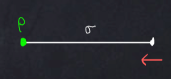
Figure 9. The bordism which computes $A_{A}$

Remark .

1. The right regular $\sigma$-module $\rho$ satisfies $\operatorname{End}_{\sigma}(\rho)\cong\sigma$, as follows from the cobordism hypothesis by the corresponding statement for algebras. See Figure 11.

2. The regular boundary theory is often called a Dirichlet boundary theory.

3. For arbitrary $(\sigma,\rho)$ acting on a field theory $F$ as in the next section, we can replace $(\sigma,\rho)$ with an algebra and its right regular module at the price of losing some dualizability; see Remark 3.2(2).

4. Not every topological field theory $\sigma$ can appear in Definition 3.1. For example, consider a 3-dimensional Reshetikhin-Turaev theory, which we assume has been extended to a fully local theory, i.e., a $(0,1,2,3)$-theory. (Usually one takes ‘Reshetikhin-Turaev theory’ to mean a $(1,2,3)$-theory, but in fact it can be made fully local [FST].) The main theorem in [FT2] asserts that “most” such theories do not admit any nonzero topological boundary theory, hence they cannot act as symmetries of a 2-dimensional field theory. (If we only assume that the Reshetikhin-Turaev theory is a $(1,2,3)$-theory, then there are possible boundary theories, at least if we include ${\mathbb{Z}}/2{\mathbb{Z}}$-gradings.) On the other hand, the Turaev-Viro theory $\sigma^{\vphantom{1*\prime y\vee M}}_{\!\Phi}$ formed from a (spherical) fusion category $\Phi$ takes values in the 3-category $\operatorname{Alg}(\operatorname{Cat})$ for a suitable 2-category $\operatorname{Cat}$ of linear categories. Thus $\sigma^{\vphantom{1*\prime y\vee M}}_{\!\Phi}$ admits the right regular $\sigma$-module defined by the right regular $\Phi$-module $\Phi^{\vphantom{1*\prime y\vee M}}_{\mkern-1.5mu\Phi}$.

5. Let $\mathscr{X}$ be a $\pi$-finite space, as in Definition A.1, and let $\sigma_{\mathscr{X}}^{(n+1)}$ be the associated $(n+1)$-dimensional topological field theory. A basepoint $*\to\mathscr{X}$ determines a right regular $\sigma$-module; see Definition A.3.2(1). This holds even if $\mathscr{X}$ is equipped with a reduced cocycle, i.e., a cocycle on the pair $(\mathscr{X},*)$. Finite group symmetries are of this type, as are finite higher group symmetries and finite 2-group symmetries.

6. Let $G$ be a finite group. Then $G$-symmetry in an $n$-dimensional quantum field theory is realized via $(n+1)$-dimensional finite gauge theory. The partition function counts principal $G$-bundles, weighted by the reciprocal of the order of the automorphism group. The regular boundary theory has an additional fluctuating field: a section of the principal $G$-bundle. Finite $G$-gauge theory can be realized as in (5) with $\mathscr{X}=BG$ a classifying space of $G$.

7. A variation on (6) is a Dijkgraaf-Witten theory [DW] in which the counting of bundles is also weighted by a characteristic number defined by a cohomology class in $H^{n+1}(BG;{\mathbb{C}}^{\times})$. For $n=1$ this class is represented by a central extension (1.9) of $G$, and the fully local field theory with values in the Morita 2-category $\operatorname{Alg}(\operatorname{Vect})$ is generated by the twisted group algebra (1.10). Observe that the passage from linear to projective symmetries (see §1.4) is not a structural change in the framework, but rather is a different choice of $(\sigma,\rho)$.

8. As in Remark 2.3(2), the topological field theory $\sigma$ need only be a once-categorified $n$-dimensional theory, not a full $(n+1)$-dimensional theory; see Example 3.3. However, a full theory may allow the possibility of more defects; see Example 4.1.

3.2. Concrete realization of topological symmetry in field theory

Let $\sigma$ be an $(n+1)$-dimensional topological field theory and let $\rho$ be a right topological $\sigma$-module. We now define a realization of the quiche $(\sigma,\rho)$ as symmetries of a quantum field theory.

Figure 10. The sandwich

Definition .

Let $(\sigma,\rho)$ be an $n$-dimensional quiche. Let $F$ be an $n$-dimensional field theory. A $(\sigma,\rho)$-module structure on $F$ is a pair $(\widetilde{F},\theta)$ in which $\widetilde{F}$ is a left $\sigma$-module and $\theta$ is an isomorphism

(3.1) $$\theta\colon\rho\otimes^{\vphantom{1*\prime y\vee M}}_{\sigma}\widetilde{F}\xrightarrow{\;\;\cong\;\;}F$$

of absolute $n$-dimensional theories.

Here ‘$\rho\otimes^{\vphantom{1*\prime y\vee M}}_{\sigma}\widetilde{F}$’ notates the dimensional reduction of $\sigma$ along the closed interval with boundaries colored with $\rho$ and $\widetilde{F}$; see Figure 10. The bulk theory $\sigma$ with its right and left boundary theories $\rho$ and $\widetilde{F}$ is sometimes called a sandwich.

Remark .

1. As in Remark 3.1(8), $\sigma$ need only be a once-categorified $n$-dimensional theory. In that case $\rho$ and $\widetilde{F}$ are relative field theories [Ste].

   

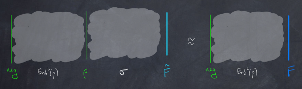
   Figure 11. The algebra $\operatorname{End}^{L}(\rho)$ acting on $F$

2. As alluded to in Remark 3.1(3), we can replace an arbitrary $\sigma$ with a theory whose value on a point is an algebra as follows. Define the 1-morphism $\rho_{1}\colon\sigma(\operatorname{pt})\to 1$ as the value of $(\sigma,\rho)$ on the bordism in Figure 9. The composition $\operatorname{End}^{L}(\rho_{1})=\rho_{1}\circ\rho_{1}^{L}$ of $\rho_{1}$ with its left adjoint is an algebra object in $\Omega\mathscr{C}$, and $\rho_{1}$ is a left $\operatorname{End}^{L}(\rho_{1})$-module; see [FT2, §2.2]. Assuming $\operatorname{End}^{L}(\rho_{1})$ is $n$-dualizable, it determines a once-categorified $n$-dimensional topological field theory $\operatorname{End}^{L}(\rho)\colon\operatorname{Bord}_{n}(\mathcal{F})\to\operatorname{Alg}(\Omega\mathscr{C})$. If we furthermore assume that the right regular module of $\operatorname{End}^{L}(\rho_{1})$ is $n$-dualizable, then it determines a right relative field theory ‘reg’ over $\operatorname{End}^{L}(\rho)$. Then as depicted in Figure 11, if $F$ has a $(\sigma,\rho)$-module structure, it also acquires a $\bigl{(}\operatorname{End}^{L}(\rho),\textnormal{regular}\bigr{)}$-module structure. These dualizability assumptions hold in many examples.

   

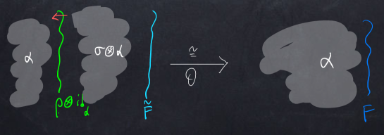
   Figure 12. The symmetry $(\sigma,\rho)$ acting on an anomalous theory

3. Definition 3.2 extends to anomalous theories $F$, or more generally to left boundary theories from some $(n+1)$-dimensional theory, as illustrated in Figure 12. In this case $\widetilde{F}$ is a left $(\sigma\otimes\alpha)$-module, and the right $(\rho\otimes\operatorname{id}_{\alpha})$-module completes the sandwich.

4. The theory $F$ and so the boundary theory $\widetilde{F}$ may be topological or nontopological, and we allow it to be not fully local (in which case we use truncations of $\sigma$ and $\rho$). We caution that there could be more topological symmetries if we do not insist on full locality of $(\sigma,\rho)$, and this can even happen if $F$ is a topological theory; see Remark 3.1(4) for an example.

5. The sandwich picture Remark 2.3 separates out the topological part $(\sigma,\rho)$ of the theory from the potentially nontopological part $\widetilde{F}$ of the theory. This is advantageous, for example in the study of defects (§4). It allows general computations in the $n$-dimensional quiche which apply to every realization as a symmetry of a field theory.

6. Typically, symmetry persists under renormalization group flow, hence a low energy approximation to $F$ should also be a $(\sigma,\rho)$-module. If $F$ is gapped, then at low energies we expect a topological theory (up to an invertible theory), so we can bring to bear powerful methods and theorems in topological field theory to investigate topological left $\sigma$-modules. This leads to dynamical predictions; see §5.

3.3. Examples

Example (quantum mechanics $n=1$).

Consider a quantum mechanical system defined by a Hilbert space $\mathscr{H}$ and a time-independent Hamiltonian $H$. The Wick-rotated theory $F$ is regarded as a map with domain $\operatorname{Bord}_{\langle 0,1\rangle}(\mathcal{F})$ for

(3.2) $$\mathcal{F}=\{\textnormal{orientation},\textnormal{Riemannian metric}\}.$$

Roughly speaking, $F(\operatorname{pt}_{+})=\mathscr{H}$ and $F(X)=e^{-\tau H/\hbar}$ for $\tau\in{\mathbb{R}}^{>0}$ and $X=[0,\tau]$ with the standard orientation and Riemannian metric. We refer to  [KS, §3] and [S2] for more precise statements.

Now suppose $G$ is a finite group equipped with a unitary representation $S\colon G\to U(\mathscr{H})$, and assume that the $G$-action commutes with the Hamiltonian $H$. To express this symmetry in terms of Definition 3.1 and Definition 3.2, let $\sigma$ be the 2-dimensional finite gauge theory with gauge group $G$. If we were only concerned with $\sigma$ we might set the codomain of $\sigma$ to be $\mathscr{C}=\operatorname{Alg}(\mathscr{C}^{\prime})$ for $\mathscr{C}^{\prime}$ the category of finite dimensional complex vector spaces and linear maps. But to accommodate the boundary theory $\widetilde{F}$ for quantum mechanics, we let $\mathscr{C}^{\prime}$ be a suitable category of topological vector spaces, as in [KS, §3]. The quiche $(\sigma,\rho)$ is defined on $\operatorname{Bord}_{2}=\operatorname{Bord}_{\langle 0,1,2\rangle}$ with no background fields. Then $\sigma(\operatorname{pt})={\mathbb{C}}[G]$ is the complex group algebra of $G$, and $\rho(\operatorname{pt})$ is its right regular module.

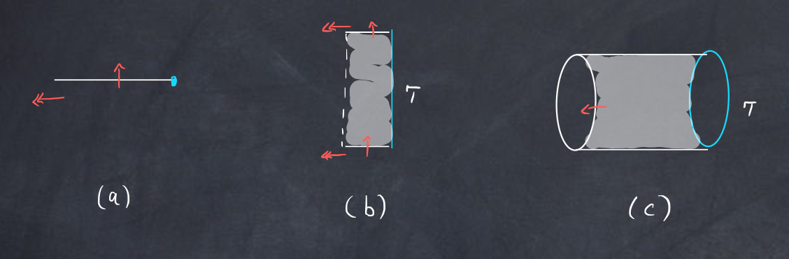
Figure 13. Three bordisms evaluated in (3.3) in the theory $(\sigma,\widetilde{F})$

Now we describe the left boundary theory $\widetilde{F}$, which has as background fields (3.2), as does the (absolute) quantum mechanical theory $F$. Observe that by cutting out a collar neighborhood it suffices to define $\widetilde{F}$ on cylinders (products with $[0,1]$) over $\widetilde{F}$-colored boundaries. The bordisms in Figure 13 do not have a well-defined width since there is a Riemannian metric only on the colored boundary. That boundary has a well-defined length $\tau$ in (b) and (c). The “arrows of time” distinguish incoming from outgoing boundaries in codimension one; we defer to [FT2, §2.1.1] for the conventions in higher codimension and for the constancy condition encoded in the dotted line in (b). Evaluation of these bordisms under $(\sigma,\widetilde{F})$ gives:

(3.3) $$\textnormal{(a)~{}the left module }{}^{\vphantom{1*\prime y\vee M}}_{{\mathbb{C}}[G]}\mathscr{H}$$

$$\textnormal{(b) }e^{-\tau H/\hbar}\colon{}^{\vphantom{1*\prime y\vee M}}_{{\mathbb{C}}[G]}\mathscr{H}\longrightarrow{}^{\vphantom{1*\prime y\vee M}}_{{\mathbb{C}}[G]}\mathscr{H}$$

(c) the central function $$g\longmapsto\operatorname{Tr}^{\vphantom{1*\prime y\vee M}}_{\mathscr{H}}\bigl{(}S(g)e^{-\tau H/\hbar}\bigr{)} G$$ on 

Assertions (a) and (b) are part of the definition of $\widetilde{F}$; it is the essential data needed to construct the nontopological $\sigma$-module $\widetilde{F}$. For (c), first note that the bordism evaluates to a class function on $G$, since $\sigma(S^{1})$ is the vector space of these class functions.

Remark .

As already mentioned in Remark 3.1(6), the finite gauge theory $\sigma$ can be constructed via a finite path integral from the $\pi$-finite space $BG$. Similarly, the boundary theory $\rho$ can be constructed from a basepoint $*\to BG$: the principal $G$-bundles are equipped with a trivialization on $\rho$-colored boundaries. A traditional picture of the $G$-symmetry of the theory $F$ uses this classical picture: the background fields $\mathcal{F}$ are augmented to $\widetilde{\mathcal{F}}=\{\textnormal{orientation},\textnormal{Riemannian metric},\textnormal{$G$-bundle}\}$, which fibers over the sheaf $\{\textnormal{$G$-bundle}\}$, so in that sense fibers over $BG$ as in §1.1. There is an absolute field theory on $\widetilde{\mathcal{F}}$ which is the “coupling of $F$ to a background gauge field” for the symmetry group $G$. The framework we are advocating here of $F$ as a $(\sigma,\rho)$-module uses the quantum finite gauge theory $\sigma$.

Remark .

The finite path integral construction of the regular (Dirichlet) boundary theory makes the isomorphism $\theta$ in (3.1) apparent. Namely, to evaluate $(\sigma,\rho)$ we sum over $G$-bundles equipped with a trivialization on $\rho$-colored boundaries. Since the trivialization propagates across an interval, the sandwich theory (Figure 10) is the original theory $F$ without the explicit $G$-symmetry.

Example (a once-categorified symmetry theory).

Let $G$ be an infinite discrete group and let ${\mathbb{C}}[G]$ be its group algebra, which we treat as untopologized. As an object in the Morita 2-category $\operatorname{Alg}(\operatorname{Vect})$ of algebras in vector spaces, ${\mathbb{C}}[G]$ is 1-dualizable but not 2-dualizable. By the cobordism hypothesis, it determines a once-categorified 1-dimensional topological field theory $\sigma$ with $\sigma(\operatorname{pt})={\mathbb{C}}[G]$. Furthermore, the right regular module ${\mathbb{C}}[G]_{{\mathbb{C}}[G]}$, regarded as a 1-morphism ${\mathbb{C}}[G]\to 1$ in $\operatorname{Alg}(\operatorname{Vect})$, has a right adjoint but not a left adjoint. Hence it determines a right relative field theory $\rho$. The pair $(\sigma,\rho)$ is a valid 1-dimensional quiche (see Remark 3.1(8)).

A similar story works for $G$ a compact Lie group. By the Peter-Weyl theorem the space of $L^{2}$ functions on $G$ is a completion of a direct sum $A_{G}$ of matrix algebras; the sum is indexed by the set of equivalence classes of irreducible representations of $G$. (If $\dim G>0$ then the direct sum $A_{G}$ is not unital; adjoin a unit to obtain a unital algebra. Its “regular” module is taken to be the direct sum without the unit.) There is a once-categorified 1-dimensional topological field theory with values in $\operatorname{Alg}(\operatorname{Vect})$ whose value on a point is $A_{G}$. In this theory the circle maps to an infinite dimensional vector space which is a sum of lines, one line for each irreducible representation of $G$.

If $G$ is an infinite discrete group or a compact Lie group, and if $\mathscr{H}$ is a Hilbert space equipped with a linear $G$-action, and $H$ is a $G$-invariant Hamiltonian, then as in Example 3.3 we can construct a left $(\sigma,\rho)$-module structure on the 1-dimensional quantum mechanical theory $F$ built from $\mathscr{H},H$. This illustrates Remark 3.2(1).

Example (full WZW).

As mentioned earlier (Remark 3.1(4)), many 3-dimensional Chern-Simons theories $\sigma^{\prime}$ do not admit nonzero fully local topological boundary theories, hence cannot act as symmetries on 2-dimensional field theories. But the doubled theory $\sigma=|\sigma^{\prime}|^{2}$ is a Turaev-Viro theory, and it can be realized with codomain $\operatorname{Alg}(\mathscr{C}^{\prime})$ for $\mathscr{C}^{\prime}$ a suitable 2-category of linear categories; see [FT2, §1.3] for example. In particular, $\sigma$ admits a right regular boundary theory $\rho$. Then the full nonchiral Wess-Zumino-Witten model $F$ (with the same group and level as the Chern-Simons theory $\sigma^{\prime}$) carries a $(\sigma,\rho)$-module structure.

Figure 14. Folding the chiral-antichiral WZW picture to obtain symmetry of full WZW

Remark .

Frequently a chiral 2-dimensional rational conformal field theory $F^{\prime}$, such as a WZW model, is viewed as a left boundary theory of a 3-dimensional topological field theory $\sigma^{\prime}$; see [Wi2, MSei2, EMSS, ADW, MSei3]. There is a conjugate anti-chiral theory $F^{\prime\prime}$ which is a right boundary theory of $\sigma^{\prime}$. There is a canonical nonchiral theory $F$ formed as the sandwich $F^{\prime\prime}\otimes_{\sigma^{\prime}}F^{\prime}$. This is called the diagonal combination of the chiral and antichiral theories. The setup in Example 3.3 is a folding in the middle, which doubles $\sigma^{\prime}$ to $\sigma$ with left boundary theory $F^{\prime\prime}\otimes F^{\prime}$; see Figure 14 in which the right regular boundary theory $\rho$ is also depicted. (Note that whereas a modular tensor category is used in the construction of $\sigma^{\prime}$, only the underlying fusion category is retained under doubling to form $\sigma$: the braiding is lost.) The right regular boundary theory $\rho$ produces the diagonal combination; any topological right boundary theory can be substituted in place of $\rho$ to form a sandwich which is a 2-dimensional conformal field theory. In some cases topological right $\sigma$-modules can be classified, and this leads to a classification of full conformal field theories obtained by combining a fixed chiral rational conformal field theory with its conjugate anti-chiral theory. The traditional approach does not use full locality, but rather uses single-valuedness of correlation functions in genera 0 and 1 (which follows automatically in our setup for oriented boundary theories); see [CIZ, MSei1, DV, KaSa, FRS] and also more more recent papers [D, E-M]. We hope to elaborate on our approach elsewhere.

Example (a homotopical symmetry).

Let $G$ be a connected compact Lie group, and suppose $A\subset G$ is a finite subgroup of the center of $G$. Let $\overline{G}=G/A$. Then a $G$-gauge theory in $n$ dimensions—for example, pure Yang-Mills theory—often has a $BA$ symmetry. In this case we take $\sigma=\sigma_{B^{2}\!A}^{(n+1)}$ to be the $A$-gerbe theory based on the $\pi$-finite space $B^{2}\!A$, and we take  $\rho$ to be the regular boundary theory constructed from a basepoint $*\to B^{2}\!A$. (See Appendix A for finite homotopy theories.) The left $\sigma$-module $\widetilde{F}$ is a $\overline{G}$-gauge theory: given an $A$-gerbe in the bulk, on the $\widetilde{F}$-boundary we sum over pairs consisting of a $\overline{G}$-connection and an isomorphism of the restricted $A$-gerbe with the obstruction to lifting the connection to a $G$-connection. Aspects of this example are discussed in more detail in [FT3, §4], and it is taken up again in [F4].

This remark extends considerably an issue that comes up in many physics papers. In a pure Yang-Mills theory with gauge group $G$ (or in a gauge theory, such as Donaldson-Witten theory, with all fields in the adjoint representation) the partition function on a manifold is constructed from the sum over principal $G$-bundles with fixed “’t Hooft flux.” Indeed, as pointed out by ’t Hooft, the partition function makes sense for such bundles. In our picture this corresponds to the insertion of a codimension two defect on the $\rho$-boundary. If we consider the same field representations, but take the gauge group to be $\overline{G}$, then when defining the partition function we sum over ’t Hooft fluxes. In the current picture, the ’t Hooft flux of the $G$-theory is fixed because of the boundary theory on the topological side of the quiche, coupled to the $\overline{G}$ theory on the right.

These examples only scratch the surface; we offer additional illustrations in §4 below. Many more examples appear in the literature.

3.4. Quotienting by a symmetry in field theory

Section 1.3 is motivation for the following.

Definition .

Let $\mathscr{C}^{\prime}$ be a symmetric monoidal $n$-category, and set $\mathscr{C}=\operatorname{Alg}(\mathscr{C}^{\prime})$. An augmentation of $A\in\mathscr{C}$ is an algebra homomorphism $\epsilon^{\vphantom{1*\prime y\vee M}}_{\mkern-1.5muA}\colon A\to 1$ from $A$ to the tensor unit $1\in\mathscr{C}$.

Thus $\epsilon^{\vphantom{1*\prime y\vee M}}_{\mkern-1.5muA}$ is a 1-morphism in $\mathscr{C}^{\prime}$ equipped with data that exhibits the structure of an algebra homomorphism. Augmentations may not exist, as in §1.4.

Remark .

A general 1-morphism $A\to 1$ in $\mathscr{C}$ is an object of $\mathscr{C}^{\prime}$ equipped with a right $A$-module structure. An augmentation is a right $A$-module structure on the tensor unit $1\in\mathscr{C}^{\prime}$.

Definition .

Let $\mathscr{C}^{\prime}$ be a symmetric monoidal $n$-category, and set $\mathscr{C}=\operatorname{Alg}(\mathscr{C}^{\prime})$. Let $\mathcal{F}$ be a collection of $(n+1)$-dimensional fields, and suppose $\sigma\colon\operatorname{Bord}_{n+1}(\mathcal{F})\to\mathscr{C}$ is a topological field theory. A right boundary theory $\epsilon$ for $\sigma$ is an augmentation of $\sigma$ if $\epsilon(\operatorname{pt})$ is an augmentation of $\sigma(\operatorname{pt})$ in the sense of Definition 3.4.

An augmentation in this sense is often called a Neumann boundary theory.

Remark .

In this context, if $\rho$ is the right regular boundary theory of $\sigma$ and $\epsilon$ is an augmentation of $\sigma$, then we can use the homomorphism $\epsilon(\operatorname{pt})\colon A\to 1$ to make $1$ into a left $A$-module, where $A=\sigma(\operatorname{pt})$, and so construct a dual left boundary theory $\epsilon^{L}$. Then the sandwich $\rho\otimes_{\sigma}\epsilon^{L}$ is the trivial theory, as follows from the cobordism hypothesis since its value on a point is $A\otimes_{A}1\cong 1$.

Example (finite path integrals).

Let $\mathscr{X}$ be a $\pi$-finite space, and let $\sigma=\sigma_{\mathscr{X}}^{(n+1)}$ be the associated topological field theory. There is a canonical Neumann boundary theory; it is the quantization of $\operatorname{id}_{\mathscr{X}}\colon\mathscr{X}\to\mathscr{X}$. See Section A.3.2.

Example (twisted version).

Continuing, suppose $\lambda\in Z^{n+1}(\mathscr{X};{\mathbb{C}}^{\times})$ is a cocycle for ordinary cohomology with ${\mathbb{C}}^{\times}$ coefficients. Recall (Definition A.3.2) that a right boundary theory may be constructed from a pair $(p,\mu)$ of a map $p\colon\mathscr{Y}\to\mathscr{X}$ of $\pi$-finite spaces and a cochain $\mu\in C^{n}(\mathscr{Y};{\mathbb{C}}^{\times})$ such that $\delta\mu=-p^{*}\lambda$. For $\mathscr{Y}=\mathscr{X}$ and $f=\operatorname{id}_{\mathscr{X}}$ the cochain $\mu$ exists iff the cohomology class $[\lambda]\in H^{n+1}(\mathscr{X};{\mathbb{C}}^{\times})$ vanishes. For example, a Dijkgraaf-Witten theory with nontrivial twisting does not admit an augmentation. If $[\lambda]=0$, and even if $\lambda=0$, then different choices of $\mu$ (up to coboundaries) yield different Neumann boundary theories. The general definition of an augmentation in this context is Definition A.3.2(2).

We use notations in Definition 3.1 and Definition 3.2 in the following.

Definition .

Suppose given an $n$-dimensional quiche $(\sigma,\rho)$ and a $(\sigma,\rho)$-module structure $(\widetilde{F},\theta)$ on a quantum field theory $F$. Suppose $\epsilon$ is an augmentation of $\sigma$. Then the quotient of $F$ by the symmetry $\sigma$ with augmentation $\epsilon$ is

(3.4) $$F\!\mkern-1.5mu\bigm{/}_{\!\mkern-1.5mu\epsilon}\!\sigma:=\epsilon\otimes_{\sigma}\widetilde{F}.$$

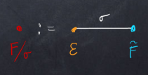
Figure 15. The quotient $F\!\mkern-1.5mu\bigm{/}_{\!\mkern-1.5mu\epsilon}\!\sigma$

The right hand side of (3.4) is the sandwich in Figure 15.

Example .

Let $G$ be a finite group, and let $\sigma=\sigma_{BG}^{(n+1)}$ be the associated finite gauge theory. Use the canonical Neumann boundary theory of Example 3.4. In the semiclassical picture this corresponds to summing over all principal $G$-bundles with no additional fields on the $\epsilon$-colored boundaries. This is the usual quotienting operation, oft called ‘gauging’.

Remark .

A nontrivial $n$-cocycle $\mu$, as in Example 3.4, induces a sum over $G$-bundles with weights, so a twisted version of the usual quotient. This twist goes by various names: ‘discrete torsion’, ‘$\theta$-angles’, etc., depending on the context. The following example is an illustration.

Example .

Picking up on Section 3.3, consider the quantum mechanical system of a particle on the Euclidean line ${\mathbb{R}}_{x}$ with Hamiltonian the Laplace operator $-d^{2}/dx^{2}$. The system is invariant under the action of the infinite discrete group ${\mathbb{Z}}$ by translations. We realize it as a theory relative to 1-dimensional once-categorified ${\mathbb{Z}}$-gauge theory. The group algebra ${\mathbb{C}}[{\mathbb{Z}}]$ has a natural augmentation (1.6), and the quotient (3.4) relative to this augmentation is the particle on the circle ${\mathbb{R}}/{\mathbb{Z}}$. Now for $\theta\in{\mathbb{R}}/2\pi{\mathbb{Z}}$ consider the character $n\mapsto e^{in\theta}$ of ${\mathbb{Z}}$. The quotient by the augmentation that corresponds to this character is the particle on the circle in the presence of a constant magnetic field.

Example .

Picking up on Section 3.3, if we replace the regular boundary theory by the augmentation $\epsilon$, then the sandwich $\epsilon\otimes_{\sigma}\widetilde{F}$ is the $\overline{G}$-gauge theory.

Example .

For $n=2$ if the codomain of $\sigma$ is a 3-category $\mathscr{C}=\operatorname{Alg}(\operatorname{Cat})$ of tensor categories, then an augmentation $A\to\operatorname{Vect}$ of the tensor category $A=\sigma(\operatorname{pt})$ is called a ‘fiber functor’. Fiber functors need not exist. For example, suppose $\lambda$ is a cocycle which represents the nonzero cohomology class in $H^{3}(B{\mathbb{Z}}/2{\mathbb{Z}};{\mathbb{C}}^{\times})$. The fusion category $\operatorname{Vect}^{\lambda}[{\mathbb{Z}}/2{\mathbb{Z}}]$ is a twisted categorified group ring of ${\mathbb{Z}}/2{\mathbb{Z}}$ with coefficients in $\operatorname{Vect}$: see [EGNO, Example 2.3.8]. (An alternative description of $\operatorname{Vect}^{\lambda}[{\mathbb{Z}}/2{\mathbb{Z}}]$ is in [FHLT, §4].) This tensor category does not admit a fiber functor [EGNO, Example 5.1.3]. The associated 3-dimensional topological field theory—a Dijkgraaf-Witten theory—with its right regular module encodes anomalous involutions on quantum field theories.

Now suppose that the codomain of $\sigma$ has the form $\mathscr{C}=\operatorname{Alg}(\mathscr{C}^{\prime})$, as in Definition 3.4, let $\rho$ be the right regular boundary theory, and suppose $\epsilon$ is a right boundary theory which is an augmentation of $\sigma$. Then there is a preferred domain wall $\delta$ from $\rho$ to $\epsilon$ as well as a preferred domain wall $\delta^{*}$ from $\epsilon$ to $\rho$.

Definition .

$\delta$  is the Dirichlet-to-Neumann domain wall, and $\delta^{*}$ is the Neumann-to-Dirichlet domain wall.

Let $F$ be an $n$-dimensional field theory equipped with a $(\sigma,\rho)$-module structure. Then $\delta$ and $\delta^{*}$ determine canonical domain walls $\delta\colon F\to F\!\mkern-1.5mu\bigm{/}_{\!\mkern-1.5mu\epsilon}\!\sigma$ and $\delta^{*}\colon F\!\mkern-1.5mu\bigm{/}_{\!\mkern-1.5mu\epsilon}\!\sigma\to F$, as depicted in Figure 16.

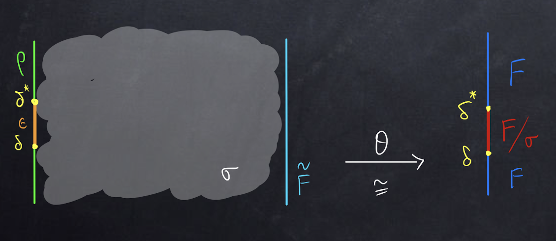
Figure 16. The canonical domain walls $\delta\colon F\to F\!\mkern-1.5mu\bigm{/}_{\!\mkern-1.5mu\epsilon}\!\sigma$ and $\delta^{*}\colon F\!\mkern-1.5mu\bigm{/}_{\!\mkern-1.5mu\epsilon}\!\sigma\to F$

3.5. Dual symmetry on a quotient; finite electromagnetic duality

In special situations a quotient theory $F\!\mkern-1.5mu\bigm{/}_{\!\mkern-1.5mu\epsilon}\!\sigma$ inherits a $(\sigma^{\vee},\rho^{\vee})$-module structure for a dual $(\sigma^{\vee},\rho^{\vee})$ to the original quiche  $(\sigma,\rho)$. One situation in which this occurs is when $\sigma$ is the field theory of a $\pi$-finite infinite loop space, or equivalently a connective $\pi$-finite spectrum; see Definition A.1. Examples include symmetries by (higher) finite abelian groups as well as by 2-groups whose $k$-invariant is a stable cohomology class. This dual symmetry is well-known in the physics literature. In low dimensions there is a precise analog for nonabelian groups [AG], [DGNO, §4.1.2], and higher dimensional generalizations have appeared recently [BSW].

Remark .

Although our exposition is confined to $\pi$-finite spectra, this duality holds more generally: for example, electromagnetic duality for general finite groups. The expectation is that the dual symmetry to a general quiche $(\sigma,\rho)$ with augmentation $\epsilon$ is the quiche which comprises $\sigma^{\vee}=\operatorname{End}_{\sigma}(\epsilon)$ with its regular module $\rho^{\vee}$; it has an augmentation $\epsilon^{\vee}=\operatorname{Hom}_{\sigma}(\rho,\epsilon)$.

Recall that if $A$ is a finite abelian group, then its Pontrjagin dual is the finite abelian group $A^{\vee}=\operatorname{Hom}(A,\mathbb{T})$. There is a similar character dual for $\pi$-finite spectra. First, define the spectrum $I\mathbb{T}$ by the universal property

(3.5) $$[\boldsymbol{X},I\mathbb{T}]\cong(\pi_{0}\boldsymbol{X})^{\vee}$$

for all spectra $\boldsymbol{X}$. (Here $[\boldsymbol{X},\boldsymbol{X}^{\prime}]$ denotes the abelian group of homotopy classes of spectrum maps $\boldsymbol{X}\to\boldsymbol{X}$.) The spectrum of maps $\boldsymbol{A}\to I\mathbb{T}$ is the character dual spectrum $\boldsymbol{A}^{\vee}$ of the $\pi$-finite spectrum $\boldsymbol{A}$; the spectrum $\boldsymbol{A}^{\vee}$ is also $\pi$-finite.

Fix $n\in{\mathbb{Z}}^{>0}$ and suppose $\boldsymbol{A}$ is a $\pi$-finite spectrum with 0-space the pointed topological space $\mathscr{X}^{\vphantom{1*\prime y\vee M}}_{\!\boldsymbol{A}}$. Let $\sigma=\sigma_{\boldsymbol{A}}^{(n+1)}$ be the corresponding $(n+1)$-dimensional topological field theory. The basepoint $*\to\mathscr{X}^{\vphantom{1*\prime y\vee M}}_{\!\boldsymbol{A}}$ determines a Dirichlet boundary theory $\rho$. The homotopy class of the duality pairing

(3.6) $$\Sigma^{n}\boldsymbol{A}^{\vee}\times\boldsymbol{A}\longrightarrow\Sigma^{n}I\mathbb{T}$$

is an $I\mathbb{T}$-cohomology class on $\mathscr{X}^{\vphantom{1*\prime y\vee M}}_{\Sigma^{n}\boldsymbol{A}^{\vee}}\times\mathscr{X}^{\vphantom{1*\prime y\vee M}}_{\!\boldsymbol{A}}$; let $\mu$ be a cocycle representative.

Definition .

1. The dual quiche $(\sigma^{\vee},\rho^{\vee})$ to $(\sigma,\rho)$ is the finite homotopy theory $\sigma^{\vee}=\sigma_{\mathscr{X}^{\vphantom{1*\prime y\vee M}}_{\Sigma^{n}\boldsymbol{A}^{\vee}}}^{(n+1)}$ with Dirichlet boundary theory $\rho^{\vee}$ defined by the basepoint $*\to\mathscr{X}^{\vphantom{1*\prime y\vee M}}_{\Sigma^{n}\boldsymbol{A}^{\vee}}$.

2. The canonical domain wall $\zeta$ between $\sigma^{\vee}$ and $\sigma$—i.e., $(\sigma^{\vee},\sigma)$-bimodule—is the finite homotopy theory constructed from the correspondence of $\pi$-finite spaces

   (3.7) $$\begin{gathered}\lx@xy@svg{\hbox{\raise 0.0pt\hbox{\kern 16.68156pt\hbox{\ignorespaces\ignorespaces\ignorespaces\hbox{\vtop{\kern 0.0pt\offinterlineskip\halign{\entry@#!@&&\entry@@#!@\cr&\\&&\crcr}}}\ignorespaces{\hbox{\kern-3.0pt\raise 0.0pt\hbox{\hbox{\kern 0.0pt\raise 0.0pt\hbox{\hbox{\kern 3.0pt\raise 0.0pt\hbox{$\textstyle{}$}}}}}}}{\hbox{\kern 40.68156pt\raise 0.0pt\hbox{\hbox{\kern 0.0pt\raise 0.0pt\hbox{\hbox{\kern 3.0pt\raise 0.0pt\hbox{$\textstyle{(\mathscr{X}^{\vphantom{1*\prime y\vee M}}_{\Sigma^{n}\boldsymbol{A}^{\vee}}\times\mathscr{X}^{\vphantom{1*\prime y\vee M}}_{\!\boldsymbol{A}},\mu)\ignorespaces\ignorespaces\ignorespaces\ignorespaces\ignorespaces\ignorespaces\ignorespaces\ignorespaces}$}}}}}}}\ignorespaces\ignorespaces\ignorespaces{}\ignorespaces\ignorespaces{\hbox{\lx@xy@drawline@}}\ignorespaces{\hbox{\kern 16.68158pt\raise-32.99765pt\hbox{\hbox{\kern 0.0pt\raise 0.0pt\hbox{\lx@xy@tip{1}\lx@xy@tip{-1}}}}}}\ignorespaces\ignorespaces{\hbox{\lx@xy@drawline@}}\ignorespaces{\hbox{\lx@xy@drawline@}}\ignorespaces\ignorespaces\ignorespaces{}\ignorespaces\ignorespaces{\hbox{\lx@xy@drawline@}}\ignorespaces{\hbox{\kern 151.43333pt\raise-33.01395pt\hbox{\hbox{\kern 0.0pt\raise 0.0pt\hbox{\lx@xy@tip{1}\lx@xy@tip{-1}}}}}}\ignorespaces\ignorespaces{\hbox{\lx@xy@drawline@}}\ignorespaces{\hbox{\lx@xy@drawline@}}{\hbox{\kern-16.68156pt\raise-41.17552pt\hbox{\hbox{\kern 0.0pt\raise 0.0pt\hbox{\hbox{\kern 3.0pt\raise 0.0pt\hbox{$\textstyle{\mathscr{X}^{\vphantom{1*\prime y\vee M}}_{\Sigma^{n}\boldsymbol{A}^{\vee}}}$}}}}}}}{\hbox{\kern 81.05745pt\raise-41.17552pt\hbox{\hbox{\kern 0.0pt\raise 0.0pt\hbox{\hbox{\kern 3.0pt\raise 0.0pt\hbox{$\textstyle{}$}}}}}}}{\hbox{\kern 151.43333pt\raise-41.17552pt\hbox{\hbox{\kern 0.0pt\raise 0.0pt\hbox{\hbox{\kern 3.0pt\raise 0.0pt\hbox{$\textstyle{\mathscr{X}^{\vphantom{1*\prime y\vee M}}_{\!\boldsymbol{A}}}$}}}}}}}\ignorespaces}}}}\ignorespaces\end{gathered} \textstyle{(\mathscr{X}^{\vphantom{1*\prime y\vee M}}_{\Sigma^{n}\boldsymbol{A}^{\vee}}\times\mathscr{X}^{\vphantom{1*\prime y\vee M}}_{\!\boldsymbol{A}},\mu)\ignorespaces\ignorespaces\ignorespaces\ignorespaces\ignorespaces\ignorespaces\ignorespaces\ignorespaces} \textstyle{\mathscr{X}^{\vphantom{1*\prime y\vee M}}_{\Sigma^{n}\boldsymbol{A}^{\vee}}} \textstyle{\mathscr{X}^{\vphantom{1*\prime y\vee M}}_{\!\boldsymbol{A}}} \textstyle{(\mathscr{X}^{\vphantom{1*\prime y\vee M}}_{\Sigma^{n}\boldsymbol{A}^{\vee}}\times\mathscr{X}^{\vphantom{1*\prime y\vee M}}_{\!\boldsymbol{A}},\mu)\ignorespaces\ignorespaces\ignorespaces\ignorespaces\ignorespaces\ignorespaces\ignorespaces\ignorespaces} \textstyle{\mathscr{X}^{\vphantom{1*\prime y\vee M}}_{\Sigma^{n}\boldsymbol{A}^{\vee}}} \textstyle{\mathscr{X}^{\vphantom{1*\prime y\vee M}}_{\!\boldsymbol{A}}}$$

   in which the maps are projections onto the factors in the Cartesian product. There is a similar canonical domain wall $\zeta^{\vee}\colon\sigma^{\vee}\to\sigma$.

3. The canonical Neumann boundary theories  $\epsilon,\epsilon^{\vee}$ are the finite homotopy theories induced from the identity maps on $\mathscr{X}^{\vphantom{1*\prime y\vee M}}_{\!\boldsymbol{A}},\mathscr{X}^{\vphantom{1*\prime y\vee M}}_{\Sigma^{n}\boldsymbol{A}^{\vee}}$, respectively.

Our formulation emphasizes the role of $\sigma$ as a symmetry for another quantum field theory. But $\sigma$ is a perfectly good $(n+1)$-dimensional field theory in its own right. From that perspective $\sigma^{\vee}$ is the $(n+1)$-dimensional electromagnetic dual theory. See [Liu] for more about electromagnetic duality in this context.

Remark .

As usual, we have not made explicit the background fields for $\sigma$, $\sigma^{\vee}$, and $\zeta$, $\zeta^{\vee}$. In fact, the theories $\sigma$ and $\sigma^{\vee}$ are defined on bordisms unadorned by background fields: they are “unoriented theories”. For $\zeta$ we need a set of (topological) background fields which orient manifolds sufficiently to integrate $\mu$. For example, if $\mu$ is a singular cocycle with coefficients in $\mathbb{T}$, then we need a usual orientation. For $I\mathbb{T}$ we would need framings.

Proposition .

There is an isomorphism of right $\sigma$-modules

(3.8) $$\psi\colon\rho^{\vee}\otimes_{\sigma^{\vee}}\zeta\xrightarrow{\;\;\cong\;\;}\epsilon$$

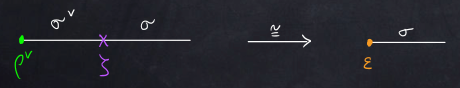
Figure 17. An isomorphism of right $\sigma$-modules

This isomorphism is depicted in Figure 17. In words, (generalized) electromagnetic duality swaps Dirichlet and Neumann boundary theories.

Proof.

We use the calculus of $\pi$-finite spectra, as described in §A.3.1—see especially the composition law (A.29). The theory $\sigma$ is induced from $\mathscr{X}^{\vphantom{1*\prime y\vee M}}_{\!\boldsymbol{A}}$, the theory $\sigma^{\vee}$ from $\mathscr{X}^{\vphantom{1*\prime y\vee M}}_{\Sigma^{n}\boldsymbol{A}^{\vee}}$, the boundary theory $\rho^{\vee}$ from $*\to\mathscr{X}^{\vphantom{1*\prime y\vee M}}_{\Sigma^{n}\boldsymbol{A}^{\vee}}$, and the domain wall $\zeta$ from the correspondence diagram (3.7). Hence $\rho^{\vee}\otimes_{\sigma^{\vee}}\zeta$ is induced from the homotopy fiber product:

(3.9) $$\begin{gathered}\lx@xy@svg{\hbox{\raise 0.0pt\hbox{\kern 5.5pt\hbox{\ignorespaces\ignorespaces\ignorespaces\hbox{\vtop{\kern 0.0pt\offinterlineskip\halign{\entry@#!@&&\entry@@#!@\cr&&\\&&&\crcr}}}\ignorespaces{\hbox{\kern-5.5pt\raise 0.0pt\hbox{\hbox{\kern 0.0pt\raise 0.0pt\hbox{\hbox{\kern 3.0pt\raise 0.0pt\hbox{$\textstyle{\ast\ignorespaces\ignorespaces\ignorespaces\ignorespaces}$}}}}}}}\ignorespaces\ignorespaces\ignorespaces{}\ignorespaces\ignorespaces{\hbox{\lx@xy@drawline@}}\ignorespaces{\hbox{\kern 39.16873pt\raise-29.42888pt\hbox{\hbox{\kern 0.0pt\raise 0.0pt\hbox{\lx@xy@tip{1}\lx@xy@tip{-1}}}}}}\ignorespaces\ignorespaces{\hbox{\lx@xy@drawline@}}\ignorespaces{\hbox{\lx@xy@drawline@}}{\hbox{\kern 29.5pt\raise 0.0pt\hbox{\hbox{\kern 0.0pt\raise 0.0pt\hbox{\hbox{\kern 3.0pt\raise 0.0pt\hbox{$\textstyle{(\mathscr{X}^{\vphantom{1*\prime y\vee M}}_{\!\boldsymbol{A}},0)\ignorespaces\ignorespaces\ignorespaces\ignorespaces\ignorespaces\ignorespaces\ignorespaces\ignorespaces}$}}}}}}}\ignorespaces\ignorespaces\ignorespaces{}\ignorespaces\ignorespaces{\hbox{\lx@xy@drawline@}}\ignorespaces{\hbox{\kern 5.50002pt\raise 0.0pt\hbox{\hbox{\kern 0.0pt\raise 0.0pt\hbox{\lx@xy@tip{1}\lx@xy@tip{-1}}}}}}\ignorespaces\ignorespaces{\hbox{\lx@xy@drawline@}}\ignorespaces{\hbox{\lx@xy@drawline@}}\ignorespaces\ignorespaces\ignorespaces{}\ignorespaces\ignorespaces{\hbox{\lx@xy@drawline@}}\ignorespaces{\hbox{\kern 104.08536pt\raise 0.0pt\hbox{\hbox{\kern 0.0pt\raise 0.0pt\hbox{\lx@xy@tip{1}\lx@xy@tip{-1}}}}}}\ignorespaces\ignorespaces{\hbox{\lx@xy@drawline@}}\ignorespaces{\hbox{\lx@xy@drawline@}}{\hbox{\kern 104.08536pt\raise 0.0pt\hbox{\hbox{\kern 0.0pt\raise 0.0pt\hbox{\hbox{\kern 3.0pt\raise 0.0pt\hbox{$\textstyle{(\mathscr{X}^{\vphantom{1*\prime y\vee M}}_{\Sigma^{n}\boldsymbol{A}^{\vee}}\times\mathscr{X}^{\vphantom{1*\prime y\vee M}}_{\!\boldsymbol{A}},\mu)\ignorespaces\ignorespaces\ignorespaces\ignorespaces\ignorespaces\ignorespaces\ignorespaces\ignorespaces}$}}}}}}}\ignorespaces\ignorespaces\ignorespaces{}\ignorespaces\ignorespaces{\hbox{\lx@xy@drawline@}}\ignorespaces{\hbox{\kern 71.47426pt\raise-33.7633pt\hbox{\hbox{\kern 0.0pt\raise 0.0pt\hbox{\lx@xy@tip{1}\lx@xy@tip{-1}}}}}}\ignorespaces\ignorespaces{\hbox{\lx@xy@drawline@}}\ignorespaces{\hbox{\lx@xy@drawline@}}\ignorespaces\ignorespaces\ignorespaces{}\ignorespaces\ignorespaces{\hbox{\lx@xy@drawline@}}\ignorespaces{\hbox{\kern 214.83713pt\raise-33.01395pt\hbox{\hbox{\kern 0.0pt\raise 0.0pt\hbox{\lx@xy@tip{1}\lx@xy@tip{-1}}}}}}\ignorespaces\ignorespaces{\hbox{\lx@xy@drawline@}}\ignorespaces{\hbox{\lx@xy@drawline@}}{\hbox{\kern-3.0pt\raise-41.17552pt\hbox{\hbox{\kern 0.0pt\raise 0.0pt\hbox{\hbox{\kern 3.0pt\raise 0.0pt\hbox{$\textstyle{}$}}}}}}}{\hbox{\kern 38.11111pt\raise-41.17552pt\hbox{\hbox{\kern 0.0pt\raise 0.0pt\hbox{\hbox{\kern 3.0pt\raise 0.0pt\hbox{$\textstyle{\mathscr{X}^{\vphantom{1*\prime y\vee M}}_{\Sigma^{n}\boldsymbol{A}^{\vee}}}$}}}}}}}{\hbox{\kern 144.46124pt\raise-41.17552pt\hbox{\hbox{\kern 0.0pt\raise 0.0pt\hbox{\hbox{\kern 3.0pt\raise 0.0pt\hbox{$\textstyle{}$}}}}}}}{\hbox{\kern 214.83713pt\raise-41.17552pt\hbox{\hbox{\kern 0.0pt\raise 0.0pt\hbox{\hbox{\kern 3.0pt\raise 0.0pt\hbox{$\textstyle{\mathscr{X}^{\vphantom{1*\prime y\vee M}}_{\!\boldsymbol{A}}}$}}}}}}}\ignorespaces}}}}\ignorespaces\end{gathered} \textstyle{\ast\ignorespaces\ignorespaces\ignorespaces\ignorespaces} \textstyle{(\mathscr{X}^{\vphantom{1*\prime y\vee M}}_{\!\boldsymbol{A}},0)\ignorespaces\ignorespaces\ignorespaces\ignorespaces\ignorespaces\ignorespaces\ignorespaces\ignorespaces} \textstyle{(\mathscr{X}^{\vphantom{1*\prime y\vee M}}_{\Sigma^{n}\boldsymbol{A}^{\vee}}\times\mathscr{X}^{\vphantom{1*\prime y\vee M}}_{\!\boldsymbol{A}},\mu)\ignorespaces\ignorespaces\ignorespaces\ignorespaces\ignorespaces\ignorespaces\ignorespaces\ignorespaces} \textstyle{\mathscr{X}^{\vphantom{1*\prime y\vee M}}_{\Sigma^{n}\boldsymbol{A}^{\vee}}} \textstyle{\mathscr{X}^{\vphantom{1*\prime y\vee M}}_{\!\boldsymbol{A}}} \textstyle{\ast\ignorespaces\ignorespaces\ignorespaces\ignorespaces} \textstyle{(\mathscr{X}^{\vphantom{1*\prime y\vee M}}_{\!\boldsymbol{A}},0)\ignorespaces\ignorespaces\ignorespaces\ignorespaces\ignorespaces\ignorespaces\ignorespaces\ignorespaces} \textstyle{(\mathscr{X}^{\vphantom{1*\prime y\vee M}}_{\Sigma^{n}\boldsymbol{A}^{\vee}}\times\mathscr{X}^{\vphantom{1*\prime y\vee M}}_{\!\boldsymbol{A}},\mu)\ignorespaces\ignorespaces\ignorespaces\ignorespaces\ignorespaces\ignorespaces\ignorespaces\ignorespaces} \textstyle{\mathscr{X}^{\vphantom{1*\prime y\vee M}}_{\Sigma^{n}\boldsymbol{A}^{\vee}}} \textstyle{\mathscr{X}^{\vphantom{1*\prime y\vee M}}_{\!\boldsymbol{A}}}$$

Here we use that the restriction of $\mu$ to $*\times\mathscr{X}^{\vphantom{1*\prime y\vee M}}_{\!\boldsymbol{A}}$ is zero. So the sandwich is the right $\sigma$-module induced from the composition

(3.10) $$\begin{gathered}\qquad\qquad\lx@xy@svg{\hbox{\raise 0.0pt\hbox{\kern 25.29268pt\hbox{\ignorespaces\ignorespaces\ignorespaces\hbox{\vtop{\kern 0.0pt\offinterlineskip\halign{\entry@#!@&&\entry@@#!@\cr&\\&&\crcr}}}\ignorespaces{\hbox{\kern-25.29268pt\raise 0.0pt\hbox{\hbox{\kern 0.0pt\raise 0.0pt\hbox{\hbox{\kern 3.0pt\raise 0.0pt\hbox{$\textstyle{(\mathscr{X}^{\vphantom{1*\prime y\vee M}}_{\!\boldsymbol{A}},0)\ignorespaces\ignorespaces\ignorespaces\ignorespaces}$}}}}}}}\ignorespaces\ignorespaces\ignorespaces{}\ignorespaces\ignorespaces{\hbox{\lx@xy@drawline@}}\ignorespaces{\hbox{\kern 49.29268pt\raise 0.0pt\hbox{\hbox{\kern 0.0pt\raise 0.0pt\hbox{\lx@xy@tip{1}\lx@xy@tip{-1}}}}}}\ignorespaces\ignorespaces{\hbox{\lx@xy@drawline@}}\ignorespaces{\hbox{\lx@xy@drawline@}}{\hbox{\kern 49.29268pt\raise 0.0pt\hbox{\hbox{\kern 0.0pt\raise 0.0pt\hbox{\hbox{\kern 3.0pt\raise 0.0pt\hbox{$\textstyle{(\mathscr{X}^{\vphantom{1*\prime y\vee M}}_{\Sigma^{n}\boldsymbol{A}^{\vee}}\times\mathscr{X}^{\vphantom{1*\prime y\vee M}}_{\!\boldsymbol{A}},\mu)\ignorespaces\ignorespaces\ignorespaces\ignorespaces}$}}}}}}}\ignorespaces\ignorespaces\ignorespaces{}\ignorespaces\ignorespaces{\hbox{\lx@xy@drawline@}}\ignorespaces{\hbox{\kern 160.04445pt\raise-32.8406pt\hbox{\hbox{\kern 0.0pt\raise 0.0pt\hbox{\lx@xy@tip{1}\lx@xy@tip{-1}}}}}}\ignorespaces\ignorespaces{\hbox{\lx@xy@drawline@}}\ignorespaces{\hbox{\lx@xy@drawline@}}{\hbox{\kern-3.0pt\raise-40.95331pt\hbox{\hbox{\kern 0.0pt\raise 0.0pt\hbox{\hbox{\kern 3.0pt\raise 0.0pt\hbox{$\textstyle{}$}}}}}}}{\hbox{\kern 89.66856pt\raise-40.95331pt\hbox{\hbox{\kern 0.0pt\raise 0.0pt\hbox{\hbox{\kern 3.0pt\raise 0.0pt\hbox{$\textstyle{}$}}}}}}}{\hbox{\kern 160.04445pt\raise-40.95331pt\hbox{\hbox{\kern 0.0pt\raise 0.0pt\hbox{\hbox{\kern 3.0pt\raise 0.0pt\hbox{$\textstyle{\mathscr{X}^{\vphantom{1*\prime y\vee M}}_{\!\boldsymbol{A}}}$}}}}}}}\ignorespaces}}}}\ignorespaces\end{gathered} \textstyle{(\mathscr{X}^{\vphantom{1*\prime y\vee M}}_{\!\boldsymbol{A}},0)\ignorespaces\ignorespaces\ignorespaces\ignorespaces} \textstyle{(\mathscr{X}^{\vphantom{1*\prime y\vee M}}_{\Sigma^{n}\boldsymbol{A}^{\vee}}\times\mathscr{X}^{\vphantom{1*\prime y\vee M}}_{\!\boldsymbol{A}},\mu)\ignorespaces\ignorespaces\ignorespaces\ignorespaces} \textstyle{\mathscr{X}^{\vphantom{1*\prime y\vee M}}_{\!\boldsymbol{A}}} \textstyle{(\mathscr{X}^{\vphantom{1*\prime y\vee M}}_{\!\boldsymbol{A}},0)\ignorespaces\ignorespaces\ignorespaces\ignorespaces} \textstyle{(\mathscr{X}^{\vphantom{1*\prime y\vee M}}_{\Sigma^{n}\boldsymbol{A}^{\vee}}\times\mathscr{X}^{\vphantom{1*\prime y\vee M}}_{\!\boldsymbol{A}},\mu)\ignorespaces\ignorespaces\ignorespaces\ignorespaces} \textstyle{\mathscr{X}^{\vphantom{1*\prime y\vee M}}_{\!\boldsymbol{A}}}$$

which is $\operatorname{id}_{\mathscr{X}^{\vphantom{1*\prime y\vee M}}_{\!\boldsymbol{A}}}$. That theory is the Neumann boundary theory $\epsilon$. ∎

Corollary .

Let $F$ be a quantum field theory equipped with a $(\sigma,\rho)$-module structure. Then the quotient $F\!\mkern-1.5mu\bigm{/}_{\!\mkern-1.5mu\epsilon}\!\sigma$ carries a canonical $(\sigma^{\vee},\rho^{\vee})$-module structure.

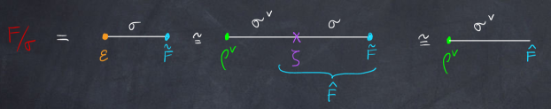
Figure 18. The dual symmetry on the quotient $F\!\mkern-1.5mu\bigm{/}_{\!\mkern-1.5mu\epsilon}\!\sigma$

Proof.

The proof is contained in Figure 18. In words: Let $(\widetilde{F},\theta)$ be the $(\sigma,\rho)$-module data, as in Definition 3.2. Define the left $\sigma^{\vee}$-module

(3.11) $$\widehat{F}=\zeta\otimes_{\sigma}\widetilde{F}$$

and the isomorphism

(3.12) $$\widehat{\theta}\colon\rho^{\vee}\otimes_{\sigma^{\vee}}\widehat{F}=\rho^{\vee}\otimes_{\sigma^{\vee}}\zeta\otimes_{\sigma}\widetilde{F}\xrightarrow{\;\;\psi\,\otimes\,\theta\;\;}\epsilon\otimes_{\sigma}\widetilde{F}=F\!\mkern-1.5mu\bigm{/}_{\!\mkern-1.5mu\epsilon}\!\sigma$$

Then $(\widehat{F},\widehat{\theta})$ is the desired $(\sigma^{\vee},\rho^{\vee})$-module structure. ∎

Remark .

The domain wall $\zeta\colon\sigma\to\sigma^{\vee}$ maps left $\sigma$-modules to left $\sigma^{\vee}$-modules; this is the effect of electromagnetic duality (on left modules). It follows from the previous that the transform of $F$ under electromagnetic duality is the quotient $F\!\mkern-1.5mu\bigm{/}_{\!\mkern-1.5mu\epsilon}\!\sigma$. This duality is involutive up to a multiplicative constant: the Euler theory; see [Liu] for details.

Example .

Let $n=2$ and let $A$ be a finite abelian group. As explained in [FT1] and many previous references, given an appropriately admissible real-valued function on $A$ there is a corresponding Ising model. It can be viewed as a 2-dimensional field theory on manifolds equipped with a lattice (appropriately defined). The group $A$ acts as a symmetry on this theory: the Ising model has a $(\sigma,\rho)$-module structure for $\sigma=\sigma_{BA}^{(3)}$ the 3-dimensional $A$-gauge theory. Finite electromagnetic duality maps $\sigma_{BA}^{(3)}$ to 3-dimensional $A^{\vee}$-gauge theory $\sigma_{BA^{\vee}}^{(3)}$. The effect on the boundary Ising model is called Kramers-Wannier duality. For $A=\mbox{$\raisebox{-0.70007pt}{\rotatebox{9.9}{\tiny{\bf/} }}\mu\raisebox{-4.2194pt}{\scalebox{2.0}{$\color[rgb]{1,1,1}\phantom{.}$}}\raisebox{3.7889pt}{$\color[rgb]{1,1,1}\phantom{.}$}\hskip 4.60007pt$}_{2}$ the admissible function is parametrized by an inverse temperature $\beta\in{\mathbb{R}}^{>0}$ and, under the canonical identification $A=A^{\vee}$, Kramers-Wannier duality amounts to an involution $\beta\leftrightarrow\beta^{\vee}$ of ${\mathbb{R}}^{>0}$. The unique fixed point $\beta^{c}$ is the critical temperature; it is the unique temperature at which the Ising model is not gapped. As another example, if $A=\mbox{$\raisebox{-0.70007pt}{\rotatebox{9.9}{\tiny{\bf/} }}\mu\raisebox{-4.2194pt}{\scalebox{2.0}{$\color[rgb]{1,1,1}\phantom{.}$}}\raisebox{3.7889pt}{$\color[rgb]{1,1,1}\phantom{.}$}\hskip 4.60007pt$}_{5}$ then there is a distinguished line in the space of admissible functions (modulo uniform scaling), which is the line of five-state Potts models. (One can replace 5 with any integer $\geq 5$ in this discussion.) There is again an involution on this line with a unique fixed point, but now the model is gapped everywhere on the line; there is a first-order phase transition at the fixed point [D-CGHMT].

4. Symmetries, defects, and composition laws

Elements of an abstract algebra $A$ act as operators on any (left) module $L$, and any equation in $A$ holds for the corresponding operators on $L$. The analogs for the quiche $(\sigma,\rho)$ in field theory are defects in $(\sigma,\rho)$ and the relations among them. Hence we begin in §4.1 with an exposition of these defects and how they transport to topological defects in a $(\sigma,\rho)$-module theory. We illustrate this concretely for finite groups of symmetries acting in quantum mechanics. We found this simple example to be quite instructive for the general story, which explains the length of our treatment in §4.2. In §4.3 we move one dimension higher, where with extra room there are new phenomena: the difference between local and global defects (Remark 4.3), defects supported on singular sets (Figure 29), etc. These examples focus on ordinary finite groups of symmetries. Our formalism easily incorporates higher groups of symmetries, as we take up in §4.4. The twistings in a higher group make the composition laws for defects more complicated than might be suspected, as we illustrate in §4.4.1. (There are many theories with a 2-group of symmetries as described in §4.4.1; see [KT, Ta, CDI, BCH] for example.) More exotic phenomena can be exhibited with a simple 2-stage spectrum, as we touch upon in §4.4.2.

4.1. Generalities

Fix a positive integer $n$. Suppose $(\sigma,\rho)$ is an $n$-dimensional quiche and $F$ is an $n$-dimensional quantum field theory equipped with a left $(\sigma,\rho)$-module structure $(\widetilde{F},\theta)$. Assume, as in §2.4, that $M$ is a $k$-dimensional manifold or bordism, $k\in\{0,1,\dots,n\}$, and $D\subset M$ is a submanifold or a stratified subspace that is the support of a defect $\delta_{D}$. Use the isomorphism (3.1) to transport the defect $\delta_{D}$ to a defect $\hat{\delta}_{D}$ supported on $[0,1]\times D\subset[0,1]\times M$ for the theory $(\sigma,\rho,\widetilde{F})$, where $\{0\}\times M$ is $\rho$-colored and $\{1\}\times M$ is $\widetilde{F}$-colored; see Figure 19.

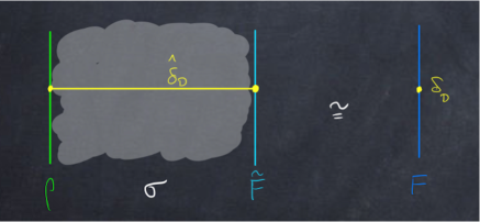
Figure 19. Transporting a defect under the isomorphism $\theta$ in (3.1)

Conversely, defects in the theory $(\sigma,\rho,\widetilde{F})$ transport to defects in $F$, but the possibilities are richer as we illustrate below. We first single out a collection of defects associated to the $(\sigma,\rho)$-symmetry.

Definition .

A $(\sigma,\rho)$-defect is a defect in the topological field theory $(\sigma,\rho)$. We call it a $\rho$-defect if its support lies entirely in a $\rho$-colored boundary.

These are defects in the abstract symmetry theory. If $F$ is a quantum field theory equipped with an $(\sigma,\rho)$-module structure $(\widetilde{F},\theta)$, then a $(\sigma,\rho)$-defect induces a defect in the theory $(\sigma,\rho,\widetilde{F})$ and hence a defect in the theory $F$. Since the defect in the sandwich picture is supported away from $\widetilde{F}$-colored boundaries, it is a topological defect in the theory $F$.

Remark .

Computations with $(\sigma,\rho)$-defects, such as compositions, are carried out in the topological field theory $(\sigma,\rho)$. They apply to the induced defects in any $(\sigma,\rho)$-module.

Remark .

Pictures such as Figure 19 are interpreted as a schematic for a tubular neighborhood of the support $D\subset M$ of the defect (and its Cartesian product with $[0,1]$). Also, unless otherwise stated, for ease of exposition we often implicitly assume a normal framing to  $D$ so that its link may be identified with a standard sphere.

The image in $F$ of a defect in the $(\sigma,\rho,\widetilde{F})$-theory might not be apparent; this is a significant advantage of the sandwich picture of $F$.

Example .

Let $n=3$ and consider a 3-dimensional quantum field theory $F$ on $S^{3}$, and assume $F$ has an $(\sigma,\rho)$-module structure. In the corresponding $(\sigma,\rho,\widetilde{F})$-theory we can contemplate a defect supported on a 2-disk $D$ in $[0,1)\times S^{3}$ whose boundary $K=\partial D\subset\{0\}\times S^{3}$ is a knot in the Dirichlet boundary. (Such a knot is termed ‘slice’.) It is possible that $K$ does not bound a disk in $S^{3}$—its Seifert genus may be positive. In this case the projection of the slice disk $D$ to a defect in the theory $F$ on $S^{3}$ is at best an immersed disk with boundary $K$, and it appears that such a topological defect is difficult to describe directly in the theory $F$. More generally, it is an open question whether all operators generated by topological defects in a full $(n+1)$-dimensional topological field theory $\sigma$ can be replicated in a once-categorified $n$-dimensional theory, even allowing for “raviolization” (Remark 2.4).

4.2. Finite symmetry in quantum mechanics

We resume consideration of the quantum mechanical theory $F$ in Example 3.3: $n=1$, the state space is a Hilbert space $\mathscr{H}$ equipped with a Hamiltonian $H$, and $H$ is invariant under the linear action of a finite group $G$ on $\mathscr{H}$. Then $\sigma$ is the 2-dimensional finite gauge theory which counts principal $G$-bundles, $\rho$ is the Dirichlet boundary theory which sums over sections of the $G$-bundle on $\rho$-colored boundaries, and $\widetilde{F}$ is constructed from the left module $\!{}^{\vphantom{1*\prime y\vee M}}_{A}\mathscr{H}$ over the group algebra $A={\mathbb{C}}[G]$. We take the codomain of $\sigma$ to be the Morita 2-category of algebras in vector spaces.

Recall from (3.3)(b) that $F\bigl{(}[0,\tau]\bigr{)}=e^{-\tau H/\hbar}$ for the standard Riemannian metric on $[0,\tau]$. Now let $D=\{t\}\subset(0,\tau)$ and suppose $\delta_{t}$ is a point defect. The link of $D\subset[0,\tau]$ is a 0-sphere $S^{0}_{\epsilon}=\{t-\epsilon,t+\epsilon\}$, and according to Remark 2.4 the point defect $\delta_{t}$ lies in the nuclear Fréchet space computed as the inverse limit

(4.1) $$\lim\limits_{\epsilon\to 0}F(S^{0}_{\epsilon});$$

see [KS, §3]. The topological vector space (4.1) can be realized as a space of operators which may be highly singular. This is what is exactly what is expected for observables in quantum theory. For our more formal purposes, we can simply treat $\delta_{t}$ as a bounded operator on $\mathscr{H}$.

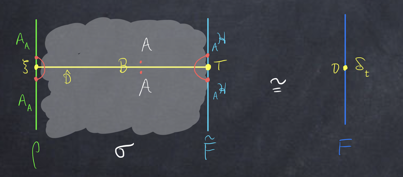
Figure 20. The point defect $\delta_{t}$ transported under the isomorphism (3.1)

Transport $\delta_{t}$ to a defect in the sandwich theory, as in Figure 20. We obtain a defect supported on the manifold-with-boundary $\widehat{D}=[0,1]\times\{t\}$, i.e., a domain wall. Treat $\widehat{D}$ as a stratified manifold and work in order of increasing codimension. First, the link of a point in the interior of $\widehat{D}$ is $S^{0}$, and $\operatorname{Hom}\bigl{(}1,\sigma(S^{0})\bigr{)}$ is the category of left $A\otimes A^{\textnormal{op}}$-modules, or equivalently of $(A,A)$-bimodules. So the label of the defect along the interior is an $(A,A)$-bimodule $\!{}^{\vphantom{1*\prime y\vee M}}_{A}B^{\vphantom{1*\prime y\vee M}}_{\mkern-1.5muA}$ . Next, the link of the endpoint on the $\rho$-colored boundary is a closed interval with interior colored with $\sigma$, boundary colored with $\rho$, and an interior point defect colored with $B$; see Figure 21. To evaluate this under $(\sigma,\rho)$, we use the rules and conventions laid out in [FT2]; they are used here in Figure 22.

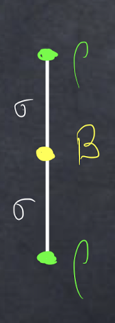
Figure 21. The link of the $\rho$-boundary point of $\widehat{D}$ in Figure 20

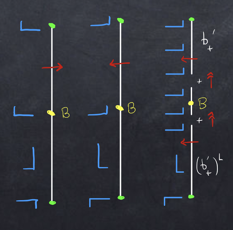
Figure 22. Evaluation of the link

(For comparison, see Figures 26 and 27 in [FT2].) In the first picture in Figure 22, then, the arrow of time points into the complement of the endpoint of the defect; see Remark 2.4. The 2-framing $f_{1},f_{2}$ is depicted as long, short. That framing is the transport of the constant framing in Figure 20; the $\pi$-rotation of the framing is a consequence of the unbending of the link. Note that our conventions require that the last framing vector point out at the $\rho$-boundary. The second picture in Figure 22 is obtained from the first by reflection in a vertical axis, so it is equivalent. The third picture expresses this bordism as a composition of bordisms glued at the $+$ point. The bordism $(b^{\prime}_{+})^{L}$ on the bottom is the left adjoint of the bordism $b^{\prime}_{+}$ on the top; see [FT2, §A.2.5]. Under $(\sigma,\rho)$, the bordism $b^{\prime}_{+}\colon+\to\emptyset^{0}$ evaluates to the right regular module $A_{A}\colon A\to 1$ in the Morita 2-category. Its left adjoint is the left $A$-module $\operatorname{Hom}_{A}(A,A)=A$. Therefore, under $(\sigma,\rho)$ the link depicted in Figure 21 evaluates to the vector space

(4.2) $$A\otimes_{A}B\otimes_{A}A\cong B.$$

Hence the label at the left endpoint of the defect in Figure 20 is a vector $\xi\in B$. At the right endpoint on the $\widetilde{F}$-colored boundary we must take a limit as the link shrinks, as in (4.1). A similar analysis to Figure 22 computes the value of this link under $(\sigma,\rho)$ as

(4.3) $$\mathscr{H}^{*}\otimes_{A}B\otimes_{A}\mathscr{H}\cong\operatorname{Hom}_{(A,A)}\bigl{(}B,\operatorname{End}(\mathscr{H})\bigr{)},$$

the space of $(A,A)$-bimodule maps $B\to\operatorname{End}(\mathscr{H})$; as remarked previously we must interpret ‘$\operatorname{End}(\mathscr{H})$’ as a space of unbounded linear operators. Let $T\colon B\to\operatorname{End}(\mathscr{H})$ be a choice of label at that endpoint. Then the image of the interval defect in the sandwich picture with labels $(\xi,B,T)$ is the point defect in the theory $F$ labeled by the operator $T(\xi)$. (It is instructive to consider the special case $B=A$—the transparent defect in the interior—in which case the defect illustrated in Figure 20 reduces to two point defects.)

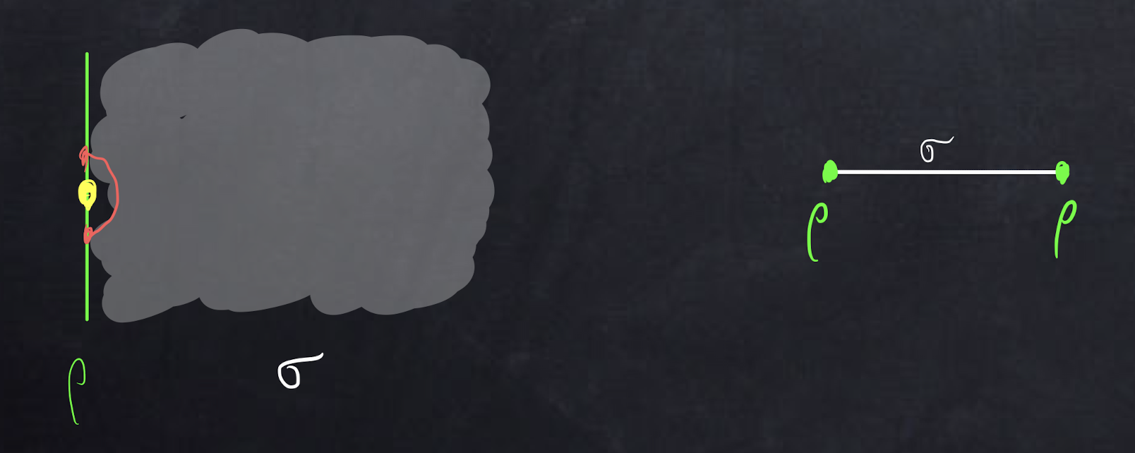
Figure 23. A point $\rho$-defect and its link

The $\widehat{D}$-defects which specialize to $(\sigma,\rho)$-defects have support disjoint from the $\widetilde{F}$-colored boundary, and so for these ${}^{\vphantom{1*\prime y\vee M}}_{A}B^{\vphantom{1*\prime y\vee M}}_{\mkern-1.5muA}=\!{}^{\vphantom{1*\prime y\vee M}}_{A}A^{\vphantom{1*\prime y\vee M}}_{\mkern-1.5muA}$ is the identity $(A,A)$-bimodule and $T=\operatorname{id}_{\mathscr{H}}$ is the identity operator. Then $\xi\in A={\mathbb{C}}[G]$. In particular, we have a defect $g\in G$ for each group element; see Figure 23. (The notion of a classical label for a defect in a finite homotopy theory is defined in Section A.3. The label $g\in G$ is an example.) Note that the link of a point defect supported on the $\rho$-colored boundary—a point $\rho$-defect—evaluates to the vector space $A\otimes_{A}A=A$. Next, consider a point $(\sigma,\rho)$-defect with support in the interior, as in Figure 24. The link is a circle $S^{1}$, and $\sigma(S^{1})$ is the center of the group algebra ${\mathbb{C}}[G]$. Here the classical labels are conjugacy classes in $G$: the label is the sum of the group elements in a conjugacy class. In particular, central elements of $G$ can label interior point defects.

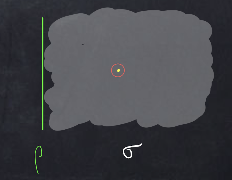
Figure 24. An interior point defect and its linking circle

Remark .

1. The point defects depicted in Figures 23 and  24 have a clear geometric interpretation in the semiclassical construction of finite gauge theory. For the point $\rho$-defect labeled by a group element $g$, the principal $G$-bundle has a trivialization on the complement of the point defect in the $\rho$-colored boundary, and the trivialization on the $\rho$-colored boundary jumps by the group element $g$ (relative to a coorientation of the point defect in the $\rho$-colored boundary). For the interior point defect labeled by a conjugacy class, the principal $G$-bundle is defined on the complement of the point and has holonomy in that conjugacy class (again relative to a coorientation of the point defect).

2. The $(\sigma,\rho)$-defects that are usually associated with $G$-symmetry are those supported on the $\rho$-colored boundary. This observation applies quite generally. Observe that these $\rho$-defects commute with defects whose support is disjoint from the $\rho$-colored boundary, since they are topological and can be homotoped on that boundary without crossing the other defects. Similarly, the defects supported in the interior commute with $\rho$-defects; this exhibits their central nature. In this example the center is smaller, so there are in a sense fewer interior $(\sigma,\rho)$-defects than there are $\rho$-defects. This is not true in higher dimensions; see §4.3.

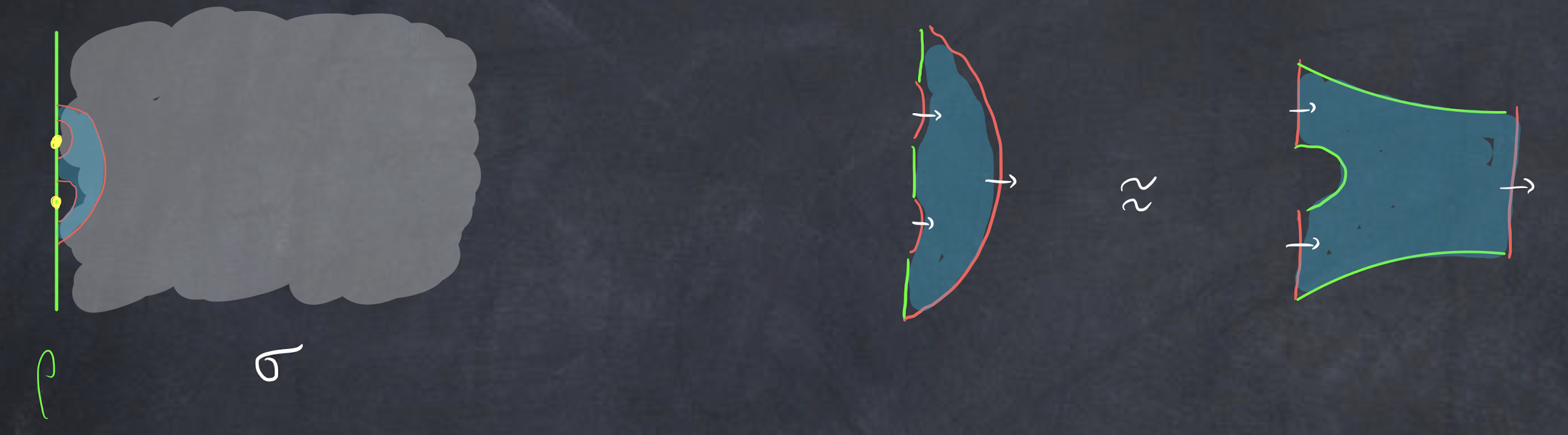
Figure 25. The composition law by evaluation on a pair of chaps

The composition law on point $\rho$-defects is computed by evaluating the “pair of chaps” in Figure 25. This works out to be the multiplication map $A\otimes A\to A$ of the group algebra; see (4.6) below. In particular, on classical labels in $G$ it restricts to the group product $G\times G\to G$.

Remark .

We make several observations that we invite the reader to apply to subsequent examples as well.

1. We can evaluate bordisms in the theory $(\sigma,\rho)$ by regarding $\sigma=\sigma_{BG}^{(2)}$ as the finite homotopy theory built from $BG$ with its basepoint $*\to BG$. So, for example, the mapping space of the link in Figure 23 is

   (4.4) $$\operatorname{Map}\bigl{(}([0,1],\{0,1\})\,,\,(BG,*)\bigr{)}\simeq\Omega BG\simeq G,$$

   which quantizes to the vector space of functions on $G$. This is canonically isomorphic to the vector space underlying the group algebra ${\mathbb{C}}[G]$. Similarly, the mapping space of the link in Figure 24 is the free loop space

   (4.5) $$\operatorname{Map}(S^{1},BG)\simeq\bigsqcup\limits_{[g]}BZ_{g},$$

   where the disjoint union runs over conjugacy classes in $G$ and $Z_{g}$ is the centralizer of a chosen element $g$ in the conjugacy class. The mapping space of the pair of chaps $C$ in Figure 25 fits into the correspondence diagram

   (4.6) $$\begin{gathered}\lx@xy@svg{\hbox{\raise 0.0pt\hbox{\kern 32.2826pt\hbox{\ignorespaces\ignorespaces\ignorespaces\hbox{\vtop{\kern 0.0pt\offinterlineskip\halign{\entry@#!@&&\entry@@#!@\cr&\\&&\crcr}}}\ignorespaces{\hbox{\kern-3.0pt\raise 0.0pt\hbox{\hbox{\kern 0.0pt\raise 0.0pt\hbox{\hbox{\kern 3.0pt\raise 0.0pt\hbox{$\textstyle{}$}}}}}}}{\hbox{\kern 56.2826pt\raise 0.0pt\hbox{\hbox{\kern 0.0pt\raise 0.0pt\hbox{\hbox{\kern 3.0pt\raise 0.0pt\hbox{$\textstyle{\operatorname{Map}\bigl{(}(C,\partial C_{\rho}),(BG,*)\bigr{)}\ignorespaces\ignorespaces\ignorespaces\ignorespaces\ignorespaces\ignorespaces\ignorespaces\ignorespaces}$}}}}}}}\ignorespaces\ignorespaces\ignorespaces{}\ignorespaces\ignorespaces{\hbox{\lx@xy@drawline@}}\ignorespaces{\hbox{\kern 27.25287pt\raise-30.0pt\hbox{\hbox{\kern 0.0pt\raise 0.0pt\hbox{\lx@xy@tip{1}\lx@xy@tip{-1}}}}}}\ignorespaces\ignorespaces{\hbox{\lx@xy@drawline@}}\ignorespaces{\hbox{\lx@xy@drawline@}}\ignorespaces\ignorespaces\ignorespaces{}\ignorespaces\ignorespaces{\hbox{\lx@xy@drawline@}}\ignorespaces{\hbox{\kern 188.55008pt\raise-33.58025pt\hbox{\hbox{\kern 0.0pt\raise 0.0pt\hbox{\lx@xy@tip{1}\lx@xy@tip{-1}}}}}}\ignorespaces\ignorespaces{\hbox{\lx@xy@drawline@}}\ignorespaces{\hbox{\lx@xy@drawline@}}{\hbox{\kern-32.2826pt\raise-39.83331pt\hbox{\hbox{\kern 0.0pt\raise 0.0pt\hbox{\hbox{\kern 3.0pt\raise 0.0pt\hbox{$\textstyle{\Omega BG\times\Omega BG}$}}}}}}}{\hbox{\kern 107.41634pt\raise-39.83331pt\hbox{\hbox{\kern 0.0pt\raise 0.0pt\hbox{\hbox{\kern 3.0pt\raise 0.0pt\hbox{$\textstyle{}$}}}}}}}{\hbox{\kern 188.55008pt\raise-39.83331pt\hbox{\hbox{\kern 0.0pt\raise 0.0pt\hbox{\hbox{\kern 3.0pt\raise 0.0pt\hbox{$\textstyle{\Omega BG}$}}}}}}}\ignorespaces}}}}\ignorespaces\end{gathered} \textstyle{\operatorname{Map}\bigl{(}(C,\partial C_{\rho}),(BG,*)\bigr{)}\ignorespaces\ignorespaces\ignorespaces\ignorespaces\ignorespaces\ignorespaces\ignorespaces\ignorespaces} \textstyle{\Omega BG\times\Omega BG} \textstyle{\Omega BG} \textstyle{\operatorname{Map}\bigl{(}(C,\partial C_{\rho}),(BG,*)\bigr{)}\ignorespaces\ignorespaces\ignorespaces\ignorespaces\ignorespaces\ignorespaces\ignorespaces\ignorespaces} \textstyle{\Omega BG\times\Omega BG} \textstyle{\Omega BG}$$

   that encodes restriction to the incoming and outgoing boundaries. Here $\partial C_{\rho}$ is the $\rho$-colored portion of $\partial C$. The left arrow in (4.6) is a homotopy equivalence and the right arrow is composition of loops. Hence the quantization of (4.6) is the convolution product of functions on $G$.

2. The computation in (4.6) generalizes to any pointed $\pi$-finite space $(\mathscr{X},*)$ in place of $(BG,*)$. (We encounter this when composing codimension one $\rho$-defects in any dimension.) Then the correspondence is multiplication on the group $\Omega\mathscr{X}$, and the quantization is pushforward under multiplication, i.e., a convolution product. If the codomain of $\sigma$ has the form $\operatorname{Alg}(\mathscr{C}^{\prime})$, then compute $\sigma(\operatorname{pt})$ as follows: (1) quantize $\Omega\mathscr{X}$ to an object in $\mathscr{C}^{\prime}$, and (2) induce the algebra structure from pushforward under multiplication $\Omega\mathscr{X}\times\Omega\mathscr{X}\to\Omega\mathscr{X}$.

3. In Figure 20, if ${}^{\vphantom{1*\prime y\vee M}}_{A}B^{\vphantom{1*\prime y\vee M}}_{\mkern-1.5muA}=\!{}^{\vphantom{1*\prime y\vee M}}_{A}A^{\vphantom{1*\prime y\vee M}}_{\mkern-1.5muA}$ is the identity $(A,A)$-bimodule and $\xi\in A$ is the unit, then $T\subset\operatorname{Hom}_{A}(\mathscr{H},\mathscr{H})$ maps to a point defect in the theory $F$ which commutes with the $G$-symmetry. (After erasing transparent defects, in the sandwich picture we have a point defect supported on the $\widetilde{F}$-boundary.) It therefore commutes with all $(\sigma,\rho)$-defects, which can be seen in the sandwich picture by moving defects up and down without collision. Similarly, an interior point defect in Figure 24 commutes with a point $\rho$-defect in Figure 23: the interior point and boundary point move freely up and down without intersection. This makes the topological nature and symmetry properties of $(\sigma,\rho)$-defects manifest.

4. Even if we begin with a group symmetry, as in this example, there are noninvertible topological $(\sigma,\rho)$-defects. Here elements of the group algebra ${\mathbb{C}}[G]$ label point defects on the $\rho$-colored boundary, and the algebra ${\mathbb{C}}[G]$ contains noninvertible elements. Also, central defects are generally noninvertible. This fits general quantum theory, which produces algebras rather than groups.

5. $(\sigma,\rho)$-defects give rise to structure in any $(\sigma,\rho)$-module: linear operators on vector spaces of point defects and on state spaces, endofunctors on categories of line defects and categories of superselection sectors, etc. These can be used to explore dynamics.

4.3. 2-dimensional theories with finite symmetry

Let $G$ be a finite group and let $\sigma$ be finite pure 3-dimensional $G$-gauge theory. As a fully local field theory, $\sigma$ can take values in $\operatorname{Alg}(\operatorname{Cat})$, a suitable 3-category of tensor categories, in which case $\sigma(\operatorname{pt})$ is the fusion category $\mathscr{A}=\operatorname{Vect}[G]$ introduced in §1.5. We can construct $\sigma$ as the finite homotopy theory $\sigma_{BG}^{(3)}$ based on the $\pi$-finite space $BG$. This is convenient for computations. The right regular boundary theory $\rho$ is constructed using the right regular module $\mathscr{A}_{\mathscr{A}}$. There are no background fields for $\sigma$ or $\rho$: the quiche $(\sigma,\rho)$ is an unoriented theory.

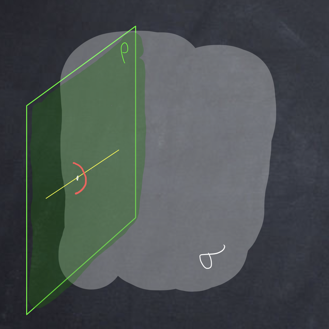
Figure 26. A line defect supported on the $\rho$-colored boundary

The most familiar $(\sigma,\rho)$-defects are the codimension 1 defects supported on the $\rho$-colored boundary, as depicted in Figure 26. The link maps under $(\sigma,\rho)$ to the quantization of the mapping space (4.4). (It is the same mapping space for the link of a codimension 1 defect in finite gauge theory of any dimension.) That quantization is a linear category, the category $\operatorname{Vect}(G)$ of vector bundles over $G$; it is the linear category which underlies the fusion category $\mathscr{A}$. The fusion product—computed from the link in Figure 27, which is the same as the link in Figure 25—is derived from the correspondence (4.6) and is the fusion product of $\mathscr{A}$. Each $g\in G$ gives rise to an invertible defect, labeled by the vector bundle over $G$ whose fiber is ${\mathbb{C}}$ at $g$ and is the zero vector space away from $g$.

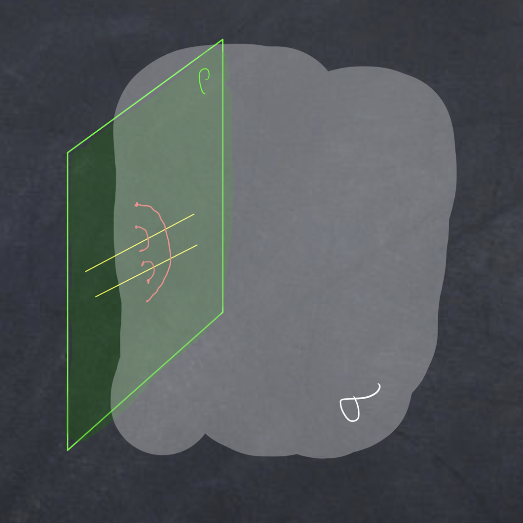
Figure 27. Fusion of line defects

Remark (${\mathbb{R}\mathbb{P}}^{1}\subset{\mathbb{R}\mathbb{P}}^{2}$).

As an illustration of how global defects may differ from local defects and from classical labels, consider the theory $(\sigma,\rho)$ on $[0,1)\times{\mathbb{R}\mathbb{P}}^{2}$ with a defect supported on $\{0\}\times{\mathbb{R}\mathbb{P}}^{1}$. The category attached to the local link is $\operatorname{Vect}(G)$, as above, but globally the link twists—the normal bundle to ${\mathbb{R}\mathbb{P}}^{1}\subset{\mathbb{R}\mathbb{P}}^{2}$ is the non-product real Möbius line bundle—so the local links quantize to a local system of categories over ${\mathbb{R}\mathbb{P}}^{1}$ with each isomorphic to $\operatorname{Vect}(G)$. The twist is by the involution induced from reflection on the linking interval. Classically this reflection inverts the parallel transport of a $G$-bundle trivialized at the endpoints of the link. Denote inversion as $\iota\colon G\to G$. The induced involution $\iota^{*}\colon\operatorname{Vect}(G)\to\operatorname{Vect}(G)$ is pullback of vector bundles. Defects supported on ${\mathbb{R}\mathbb{P}}^{1}$ have a global label which is a section of this local system, or equivalently a (homotopy) fixed point of the involution $\iota^{*}$, i.e., an $\iota$-equivariant vector bundle over $G$. The invertible defects are trivial lines supported at elements of order dividing two.

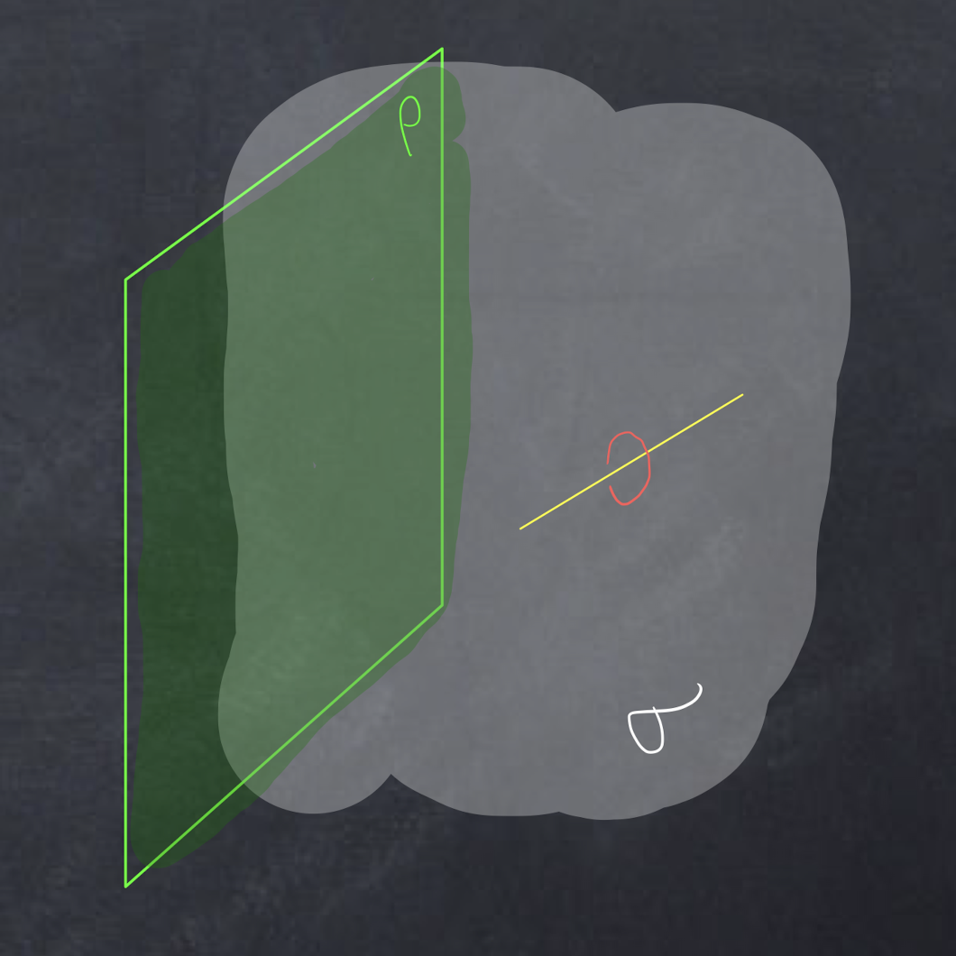
Figure 28. A line defect supported in the bulk

Now consider a line defect supported in the bulk, as in Figure 28. The link is a circle, and so a local defect is an object in the category $\sigma(S^{1})=\operatorname{Vect}_{G}(G)$ of $G$-equivariant vector bundles over $G$. (Here $G$ acts on itself via conjugation.) This is the (Drinfeld) center of $\mathscr{A}$. Note that unlike the case $n=2$—see Remark 4.2(2)—the center here is “larger” than the algebra $\mathscr{A}$. The simple objects of the center are labeled by a pair consisting of a conjugacy class and an irreducible representation of the centralizer of an element in the conjugacy class. The corresponding defect is invertible iff the representation is 1-dimensional. Among these defects are the Wilson and ’t Hooft lines of the 3-dimensional $G$-gauge theory. There is a rich set of topological defects that goes beyond those labeled by group elements.

Remark .

The reader can check that the only non-transparent point defects are scalar multiples of the identity.

Remark .

A variation includes a twist of the pure $G$-gauge theory via a cocycle representing a class in $H^{3}(BG;{\mathbb{C}}^{\times})$. This is also a finite homotopy theory, first studied by Dijkgraaf-Witten [DW]. There is a regular boundary theory $\rho$, but there is not a fiber functor, as already mentioned in §1.5.

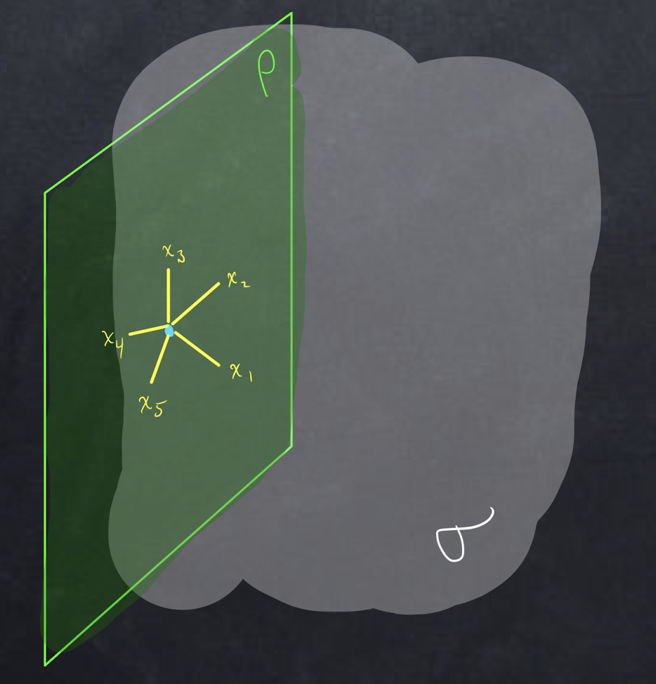
Figure 29. A stratified $\rho$-defect

The example of finite $G$-gauge theory generalizes to arbitrary Turaev-Viro theories. Let $\Phi$ be a spherical fusion category, let $\sigma$ be the induced 3-dimensional topological field theory (of oriented bordisms) with $\sigma(\operatorname{pt})=\Phi$, and define the regular boundary theory $\rho$ via the right regular module $\Phi_{\Phi}$. The category of line $\rho$-defects is the linear category which underlies $\Phi$, so a defect is labeled (locally) by an object of $\Phi$. The fusion product is the tensor product in $\Phi$. We can also have nontrivial stratified $\rho$-defects, such as illustrated in Figure 29. In the figure the $x_{i}$ are objects of $\Phi$ and the label at the central point is a vector in $\operatorname{Hom}_{\Phi}(1,x_{1}\otimes\cdots\otimes x_{5})$.

4.4. Higher group symmetries: composition of defects

The two examples in this section demonstrate that in general there is no sensible composition law on classical labels in finite homotopy theories. (See Section A.3 for a definition of classical labels.) We illustrate that nonzero $k$-invariants manifest as higher multiplicative structures in the categories obtained by quantization. We will also emphasize both at the semiclassical and quantum levels how automorphisms of local defects play a role in their globalization by means of the topology of the normal bundle. (See Section 4.3 for an example of this phenomenon.)

4.4.1. A 2-group example

Let $G$ be a finite group, let $A$ be a finite abelian group, and fix a cocycle $k$ for a cohomology class $[k]\in H^{3}(G;A)$. (We leave the reader to include a nontrivial $G$-action on $A$ in what follows.) Realize $k$ as a map $k\colon BG\to B^{3}\mkern-1.5muA$, and form the $\pi$-finite space $\mathscr{X}$ as a pullback:

(4.7) $$\begin{gathered}\lx@xy@svg{\hbox{\raise 0.0pt\hbox{\kern 11.77675pt\hbox{\ignorespaces\ignorespaces\ignorespaces\hbox{\vtop{\kern 0.0pt\offinterlineskip\halign{\entry@#!@&&\entry@@#!@\cr&\\&\\&\crcr}}}\ignorespaces{\hbox{\kern-11.77675pt\raise 0.0pt\hbox{\hbox{\kern 0.0pt\raise 0.0pt\hbox{\hbox{\kern 3.0pt\raise 0.0pt\hbox{$\textstyle{B^{2}\mkern-1.5muA\ignorespaces\ignorespaces\ignorespaces\ignorespaces\ignorespaces\ignorespaces\ignorespaces\ignorespaces}$}}}}}}}\ignorespaces\ignorespaces\ignorespaces\ignorespaces{}{\hbox{\hbox{\kern 0.0pt\raise 1.0pt\hbox{\lx@xy@droprule}}\hbox{\kern 0.0pt\raise-1.0pt\hbox{\lx@xy@droprule}}}}\ignorespaces{}{\hbox{\hbox{\kern 0.0pt\raise 1.0pt\hbox{\lx@xy@droprule}}\hbox{\kern 0.0pt\raise-1.0pt\hbox{\lx@xy@droprule}}}}{\hbox{\hbox{\kern 0.0pt\raise 1.0pt\hbox{\lx@xy@droprule}}\hbox{\kern 0.0pt\raise-1.0pt\hbox{\lx@xy@droprule}}}}\ignorespaces\ignorespaces\ignorespaces\ignorespaces{}{\hbox{\lx@xy@droprule}}\ignorespaces{\hbox{\kern 0.0pt\raise-27.90222pt\hbox{\hbox{\kern 0.0pt\raise 0.0pt\hbox{\lx@xy@tip{1}\lx@xy@tip{-1}}}}}}{\hbox{\lx@xy@droprule}}{\hbox{\lx@xy@droprule}}{\hbox{\kern 53.77675pt\raise 0.0pt\hbox{\hbox{\kern 0.0pt\raise 0.0pt\hbox{\hbox{\kern 3.0pt\raise 0.0pt\hbox{$\textstyle{B^{2}\mkern-1.5muA\ignorespaces\ignorespaces\ignorespaces\ignorespaces}$}}}}}}}\ignorespaces\ignorespaces\ignorespaces\ignorespaces{}{\hbox{\lx@xy@droprule}}\ignorespaces{\hbox{\kern 65.5535pt\raise-30.08275pt\hbox{\hbox{\kern 0.0pt\raise 0.0pt\hbox{\lx@xy@tip{1}\lx@xy@tip{-1}}}}}}{\hbox{\lx@xy@droprule}}{\hbox{\lx@xy@droprule}}{\hbox{\kern-6.75pt\raise-37.73553pt\hbox{\hbox{\kern 0.0pt\raise 0.0pt\hbox{\hbox{\kern 3.0pt\raise 0.0pt\hbox{$\textstyle{\mathscr{X}\ignorespaces\ignorespaces\ignorespaces\ignorespaces\ignorespaces\ignorespaces\ignorespaces\ignorespaces}$}}}}}}}\ignorespaces\ignorespaces\ignorespaces{}\ignorespaces\ignorespaces{\hbox{\lx@xy@drawline@}}\ignorespaces{\hbox{\kern 60.0535pt\raise-37.73553pt\hbox{\hbox{\kern 0.0pt\raise 0.0pt\hbox{\lx@xy@tip{1}\lx@xy@tip{-1}}}}}}\ignorespaces\ignorespaces{\hbox{\lx@xy@drawline@}}\ignorespaces{\hbox{\lx@xy@drawline@}}\ignorespaces\ignorespaces\ignorespaces\ignorespaces{}{\hbox{\lx@xy@droprule}}\ignorespaces{\hbox{\kern 0.0pt\raise-65.63776pt\hbox{\hbox{\kern 0.0pt\raise 0.0pt\hbox{\lx@xy@tip{1}\lx@xy@tip{-1}}}}}}{\hbox{\lx@xy@droprule}}{\hbox{\lx@xy@droprule}}{\hbox{\kern 60.0535pt\raise-37.73553pt\hbox{\hbox{\kern 0.0pt\raise 0.0pt\hbox{\hbox{\kern 3.0pt\raise 0.0pt\hbox{$\textstyle{\ast\ignorespaces\ignorespaces\ignorespaces\ignorespaces}$}}}}}}}\ignorespaces\ignorespaces\ignorespaces\ignorespaces{}{\hbox{\lx@xy@droprule}}\ignorespaces{\hbox{\kern 65.5535pt\raise-63.83331pt\hbox{\hbox{\kern 0.0pt\raise 0.0pt\hbox{\lx@xy@tip{1}\lx@xy@tip{-1}}}}}}{\hbox{\lx@xy@droprule}}{\hbox{\lx@xy@droprule}}{\hbox{\kern-10.97464pt\raise-75.47107pt\hbox{\hbox{\kern 0.0pt\raise 0.0pt\hbox{\hbox{\kern 3.0pt\raise 0.0pt\hbox{$\textstyle{BG\ignorespaces\ignorespaces\ignorespaces\ignorespaces}$}}}}}}}\ignorespaces\ignorespaces\ignorespaces\ignorespaces{}{\hbox{\lx@xy@droprule}}\ignorespaces\ignorespaces\ignorespaces{\hbox{\kern 27.84447pt\raise-70.04051pt\hbox{{}\hbox{\kern 0.0pt\raise 0.0pt\hbox{\hbox{\kern 3.0pt\hbox{\hbox{\kern 0.0pt\raise-2.43056pt\hbox{$\scriptstyle{k}$}}}\kern 3.0pt}}}}}}\ignorespaces{\hbox{\kern 53.77675pt\raise-75.47107pt\hbox{\hbox{\kern 0.0pt\raise 0.0pt\hbox{\lx@xy@tip{1}\lx@xy@tip{-1}}}}}}{\hbox{\lx@xy@droprule}}{\hbox{\lx@xy@droprule}}{\hbox{\kern 53.77675pt\raise-75.47107pt\hbox{\hbox{\kern 0.0pt\raise 0.0pt\hbox{\hbox{\kern 3.0pt\raise 0.0pt\hbox{$\textstyle{B^{3}\mkern-1.5muA}$}}}}}}}\ignorespaces}}}}\ignorespaces\end{gathered} \textstyle{B^{2}\mkern-1.5muA\ignorespaces\ignorespaces\ignorespaces\ignorespaces\ignorespaces\ignorespaces\ignorespaces\ignorespaces} \textstyle{B^{2}\mkern-1.5muA\ignorespaces\ignorespaces\ignorespaces\ignorespaces} \textstyle{\mathscr{X}\ignorespaces\ignorespaces\ignorespaces\ignorespaces\ignorespaces\ignorespaces\ignorespaces\ignorespaces} \textstyle{\ast\ignorespaces\ignorespaces\ignorespaces\ignorespaces} \textstyle{BG\ignorespaces\ignorespaces\ignorespaces\ignorespaces} \scriptstyle{k} \textstyle{B^{3}\mkern-1.5muA} \textstyle{B^{2}\mkern-1.5muA\ignorespaces\ignorespaces\ignorespaces\ignorespaces\ignorespaces\ignorespaces\ignorespaces\ignorespaces} \textstyle{B^{2}\mkern-1.5muA\ignorespaces\ignorespaces\ignorespaces\ignorespaces} \textstyle{\mathscr{X}\ignorespaces\ignorespaces\ignorespaces\ignorespaces\ignorespaces\ignorespaces\ignorespaces\ignorespaces} \textstyle{\ast\ignorespaces\ignorespaces\ignorespaces\ignorespaces} \textstyle{BG\ignorespaces\ignorespaces\ignorespaces\ignorespaces} \scriptstyle{k} \textstyle{B^{3}\mkern-1.5muA}$$

Then $\mathscr{X}$ is the classifying space of a 2-group $\Omega\mathscr{X}$ which is an extension of $G$ by $BA$. Note that $BA$ is the sub and $G$ is the quotient. The extension class is $[k]\in H^{3}(G;A)\cong H^{2}(G;BA)$. A nonzero $[k]$ means the extension is not split, in which case $\Omega\mathscr{X}$ is not the product 2-group. We do not use the 2-group directly, but rather use its classifying space $\mathscr{X}$. Maps into $\mathscr{X}$ are “background gauge fields” for the 2-group symmetry.

Set $n=2$ and let $\sigma=\sigma_{\mathscr{X}}^{(3)}$ be the finite homotopy theory built from $\mathscr{X}$. It has a regular boundary theory $\rho$ as the quantization of a basepoint $*\to\mathscr{X}$. Let the codomain of $\sigma$ be $\operatorname{Alg}(\operatorname{Cat})$, a 3-category of tensor categories; the domain is the bordism category $\operatorname{Bord}_{3}$ of unoriented manifolds. The tensor category $\sigma(\operatorname{pt})$ is obtained by quantizing $\mathscr{X}$. One way to compute it, based on Remark 4.2(2), is to quantize $\Omega\mathscr{X}$ to a linear category and induce the monoidal structure from multiplication on $\Omega\mathscr{X}$. First assume $G=1$, so that $\mathscr{X}=B^{2}\mkern-1.5muA$ and $\Omega\mathscr{X}$ is the homotopical group $BA$. The category of (flat) vector bundles on $\Omega\mathscr{X}=BA$ is $\operatorname{Rep}(A)$, the category of linear representations of $A$. The monoidal structure induced by multiplication on $BA$ is not the usual tensor product of representations. Rather, identify $\operatorname{Rep}(A)\simeq\operatorname{Vect}(A^{\vee})$, where $\operatorname{Vect}(A^{\vee})$ is the category of vector bundles on the Pontrjagin dual group. The monoidal structure on $\operatorname{Vect}(A^{\vee})$ is pointwise tensor product. Denote this tensor category as ‘$\operatorname{Rep}_{c}(A)$’. Observe that the tensor unit is the trivial line bundle on $\operatorname{Vect}(A^{\vee})$ with fiber ${\mathbb{C}}$, which corresponds to the regular representation of $A$ in $\operatorname{Rep}_{c}(A)$. For general finite $G$, but zero $k$-invariant, the quantization is the group ring of $G$ with coefficients in $\operatorname{Rep}_{c}(A)$, which we denote $\operatorname{Rep}_{c}(A)[G]$. The objects of the underlying linear category $\mathcal{L}$ are vector bundles on $G$ whose fibers are representations of $A$, or equivalently the fibers are vector bundles over $A^{\vee}$. A $k$-invariant $[k]\in H^{3}(G;A)\cong H^{2}(G;BA)$ can be represented as a principal $A$-bundle $K\to G\times G$—compare [FHLT, §4.1]—together with further cocycle data/conditions. Observe that an $A$-torsor $K_{g_{1},g_{2}}$ produces a complex line bundle $L_{g_{1},g_{2}}\to A^{\vee}$. So there is a twisted convolution product: if $W_{i}\to G$, $i=1,2$, are bundles over $G$ whose fibers are vector bundles over $A^{\vee}$, then define

(4.8) $$(W_{1}*W_{2})_{g}=\bigoplus\limits_{g_{1}g_{2}=g}L_{g_{1},g_{2}}\otimes(W_{1})_{g_{1}}\otimes(W_{2})_{g_{2}},\qquad g\in G.$$

This produces a tensor category $\mathscr{T}=\operatorname{Rep}_{c}(A)_{k}[G]$; it is the desired quantization of $\mathscr{X}$. The tensor unit 1 is the vector bundle over $G$ supported at $e\in G$ with fiber the regular representation of $A$. Notice that $\operatorname{Hom}_{\mathscr{T}}(1,1)$ is the vector space underlying this representation, the vector space $\operatorname{Fun}(A)$ of functions $A\to{\mathbb{C}}$, and it carries the algebra structure of the group algebra.

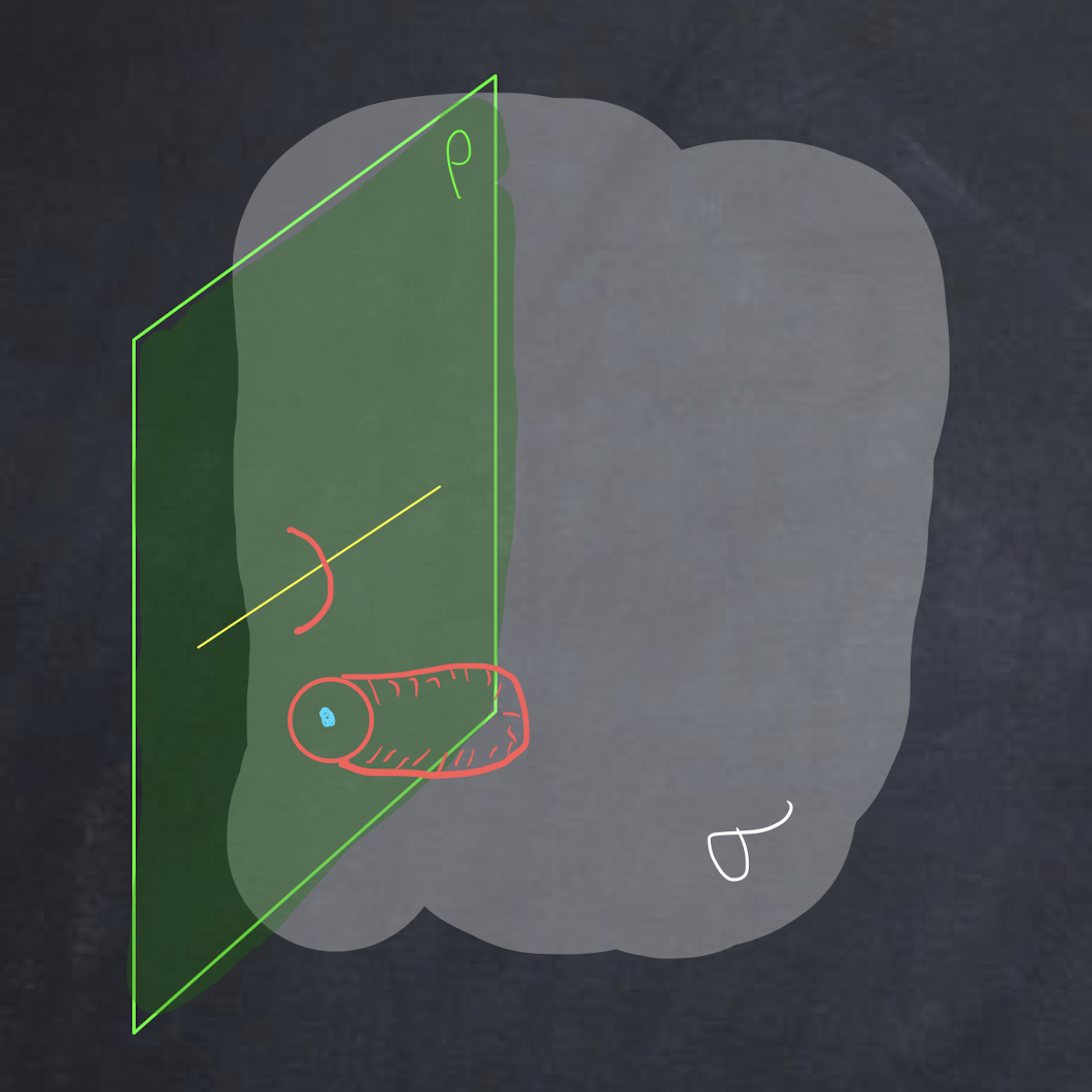
Figure 30. A point defect and a line defect on the $\rho$-colored boundary

Now consider point and line $\rho$-defects, as illustrated together with their links in Figure 30. The mapping spaces of these links into $\mathscr{X}$ are—respectively for the point defect and line defect—the (iterated) based loop spaces

(4.9) $$\Omega^{2}\mathscr{X} \simeq A$$

(4.10) $$\Omega\mathscr{X} \simeq G\times BA$$

(See (4.4) for more detail.) The classical labels for invertible defects are—respectively for the point defects and line defects—elements of the abelian group $A$ and of the group $G$. The quantizations are the vector space $\operatorname{Hom}_{\mathscr{T}}(1,1)$ and the linear category $\mathcal{L}$, respectively:

(4.11) $$\operatorname{Fun}(A)$$

(4.12) $$\mathcal{L}=\operatorname{Vect}(G)\times\operatorname{Rep}(A)$$

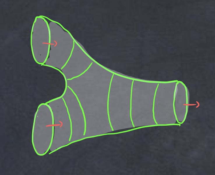
Figure 31. Computation of the fusion rule for point defects

The (quantum) composition law on point defects is computed by quantization of a 3-dimensional pair of chaps $S$, which can also be described as a solid pair of pants: see Figure 31. From the correspondence

(4.13) $$\begin{gathered}\lx@xy@svg{\hbox{\raise 0.0pt\hbox{\kern 25.52223pt\hbox{\ignorespaces\ignorespaces\ignorespaces\hbox{\vtop{\kern 0.0pt\offinterlineskip\halign{\entry@#!@&&\entry@@#!@\cr&\\&&\crcr}}}\ignorespaces{\hbox{\kern-3.0pt\raise 0.0pt\hbox{\hbox{\kern 0.0pt\raise 0.0pt\hbox{\hbox{\kern 3.0pt\raise 0.0pt\hbox{$\textstyle{}$}}}}}}}{\hbox{\kern 49.52223pt\raise 0.0pt\hbox{\hbox{\kern 0.0pt\raise 0.0pt\hbox{\hbox{\kern 3.0pt\raise 0.0pt\hbox{$\textstyle{\operatorname{Map}(S,\mathscr{X})\ignorespaces\ignorespaces\ignorespaces\ignorespaces\ignorespaces\ignorespaces\ignorespaces\ignorespaces}$}}}}}}}\ignorespaces\ignorespaces\ignorespaces{}\ignorespaces\ignorespaces{\hbox{\lx@xy@drawline@}}\ignorespaces{\hbox{\kern 21.82079pt\raise-28.09778pt\hbox{\hbox{\kern 0.0pt\raise 0.0pt\hbox{\lx@xy@tip{1}\lx@xy@tip{-1}}}}}}\ignorespaces\ignorespaces{\hbox{\lx@xy@drawline@}}\ignorespaces{\hbox{\lx@xy@drawline@}}\ignorespaces\ignorespaces\ignorespaces{}\ignorespaces\ignorespaces{\hbox{\lx@xy@drawline@}}\ignorespaces{\hbox{\kern 123.45287pt\raise-32.05176pt\hbox{\hbox{\kern 0.0pt\raise 0.0pt\hbox{\lx@xy@tip{1}\lx@xy@tip{-1}}}}}}\ignorespaces\ignorespaces{\hbox{\lx@xy@drawline@}}\ignorespaces{\hbox{\lx@xy@drawline@}}{\hbox{\kern-25.52223pt\raise-39.73553pt\hbox{\hbox{\kern 0.0pt\raise 0.0pt\hbox{\hbox{\kern 3.0pt\raise 0.0pt\hbox{$\textstyle{\Omega^{2}\mathscr{X}\times\Omega^{2}\mathscr{X}}$}}}}}}}{\hbox{\kern 71.48755pt\raise-39.73553pt\hbox{\hbox{\kern 0.0pt\raise 0.0pt\hbox{\hbox{\kern 3.0pt\raise 0.0pt\hbox{$\textstyle{}$}}}}}}}{\hbox{\kern 123.45287pt\raise-39.73553pt\hbox{\hbox{\kern 0.0pt\raise 0.0pt\hbox{\hbox{\kern 3.0pt\raise 0.0pt\hbox{$\textstyle{\Omega^{2}\mathscr{X}}$}}}}}}}\ignorespaces}}}}\ignorespaces\end{gathered} \textstyle{\operatorname{Map}(S,\mathscr{X})\ignorespaces\ignorespaces\ignorespaces\ignorespaces\ignorespaces\ignorespaces\ignorespaces\ignorespaces} \textstyle{\Omega^{2}\mathscr{X}\times\Omega^{2}\mathscr{X}} \textstyle{\Omega^{2}\mathscr{X}} \textstyle{\operatorname{Map}(S,\mathscr{X})\ignorespaces\ignorespaces\ignorespaces\ignorespaces\ignorespaces\ignorespaces\ignorespaces\ignorespaces} \textstyle{\Omega^{2}\mathscr{X}\times\Omega^{2}\mathscr{X}} \textstyle{\Omega^{2}\mathscr{X}}$$

which is essentially the diagram for the group law on $\pi_{2}\mathscr{X}$, we deduce the commutative algebra structure of convolution on $\operatorname{Fun}(A)$, which is then the group algebra ${\mathbb{C}}[A]$. Therefore, for point defects the composition law for quantum defects, labeled by elements of the vector space $\operatorname{Fun}(A)$, specializes to multiplication on $A$, which is the natural composition law on classical labels.

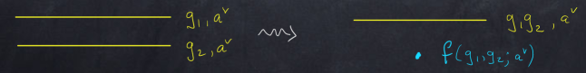
Figure 32. A putative composition law on labels for line defects

Now consider line defects. Recall that classical labels—path components in (4.10)—are elements of $G$ and their composition law is multiplication in $G$. By contrast, the set of isomorphism classes of simple objects in the category $\mathcal{L}$ in (4.12) is $G\times A^{\vee}$. Under the tensor structure on $\mathcal{L}$, given in (4.8), the product of two simples is simple; the induced composition law on $G\times A^{\vee}$ is the group law of $G$ on $G\times\{a^{\vee}\}$ for all $a^{\vee}\in A^{\vee}$.

If the $k$-invariant vanishes, so the symmetry group splits as $G\times BA$, then simple line defects compose as just described; see §4.3. The general composition law, which is based on quantum labels, is computed from the pair of chaps $C$, as in Figure 25. It leads to the correspondence

(4.14) $$\begin{gathered}\lx@xy@svg{\hbox{\raise 0.0pt\hbox{\kern 22.72223pt\hbox{\ignorespaces\ignorespaces\ignorespaces\hbox{\vtop{\kern 0.0pt\offinterlineskip\halign{\entry@#!@&&\entry@@#!@\cr&\\&&\crcr}}}\ignorespaces{\hbox{\kern-3.0pt\raise 0.0pt\hbox{\hbox{\kern 0.0pt\raise 0.0pt\hbox{\hbox{\kern 3.0pt\raise 0.0pt\hbox{$\textstyle{}$}}}}}}}{\hbox{\kern 46.72223pt\raise 0.0pt\hbox{\hbox{\kern 0.0pt\raise 0.0pt\hbox{\hbox{\kern 3.0pt\raise 0.0pt\hbox{$\textstyle{\operatorname{Map}(C,\mathscr{X})\ignorespaces\ignorespaces\ignorespaces\ignorespaces\ignorespaces\ignorespaces\ignorespaces\ignorespaces}$}}}}}}}\ignorespaces\ignorespaces\ignorespaces{}\ignorespaces\ignorespaces{\hbox{\lx@xy@drawline@}}\ignorespaces{\hbox{\kern 18.30301pt\raise-29.0pt\hbox{\hbox{\kern 0.0pt\raise 0.0pt\hbox{\lx@xy@tip{1}\lx@xy@tip{-1}}}}}}\ignorespaces\ignorespaces{\hbox{\lx@xy@drawline@}}\ignorespaces{\hbox{\lx@xy@drawline@}}\ignorespaces\ignorespaces\ignorespaces{}\ignorespaces\ignorespaces{\hbox{\lx@xy@drawline@}}\ignorespaces{\hbox{\kern 121.80704pt\raise-32.12491pt\hbox{\hbox{\kern 0.0pt\raise 0.0pt\hbox{\lx@xy@tip{1}\lx@xy@tip{-1}}}}}}\ignorespaces\ignorespaces{\hbox{\lx@xy@drawline@}}\ignorespaces{\hbox{\lx@xy@drawline@}}{\hbox{\kern-22.72223pt\raise-38.83331pt\hbox{\hbox{\kern 0.0pt\raise 0.0pt\hbox{\hbox{\kern 3.0pt\raise 0.0pt\hbox{$\textstyle{\Omega\mathscr{X}\times\Omega\mathscr{X}}$}}}}}}}{\hbox{\kern 69.26463pt\raise-38.83331pt\hbox{\hbox{\kern 0.0pt\raise 0.0pt\hbox{\hbox{\kern 3.0pt\raise 0.0pt\hbox{$\textstyle{}$}}}}}}}{\hbox{\kern 121.80704pt\raise-38.83331pt\hbox{\hbox{\kern 0.0pt\raise 0.0pt\hbox{\hbox{\kern 3.0pt\raise 0.0pt\hbox{$\textstyle{\Omega\mathscr{X}}$}}}}}}}\ignorespaces}}}}\ignorespaces\end{gathered} \textstyle{\operatorname{Map}(C,\mathscr{X})\ignorespaces\ignorespaces\ignorespaces\ignorespaces\ignorespaces\ignorespaces\ignorespaces\ignorespaces} \textstyle{\Omega\mathscr{X}\times\Omega\mathscr{X}} \textstyle{\Omega\mathscr{X}} \textstyle{\operatorname{Map}(C,\mathscr{X})\ignorespaces\ignorespaces\ignorespaces\ignorespaces\ignorespaces\ignorespaces\ignorespaces\ignorespaces} \textstyle{\Omega\mathscr{X}\times\Omega\mathscr{X}} \textstyle{\Omega\mathscr{X}}$$

which induces a tensor structure on the quantization of $\Omega\mathscr{X}\simeq G\times BA$. By Remark 4.2(2) this recovers $\sigma(\operatorname{pt})$, namely the tensor category $\mathscr{T}=\operatorname{Rep}_{c}(A)_{k}[G]$ with its monoidal structure (4.8). This is the correct composition law on line defects. The important point is that the cocycle $k$ is part of the tensor structure; if $[k]\neq 0$ then whereas the space $\Omega\mathscr{X}$ is a Cartesian product, the group $\mathscr{X}$ is not a direct product: it is a nonsplit 2-group. A choice of splitting $\Omega\mathscr{X}\simeq G\times BA$ as a space does not lead to the group law on $G$, which is the quotient of the 2-group $\Omega\mathscr{X}$ by the subgroup $BA$. (This is apparent in the model $K\to G\times G$ for the $k$-invariant given before (4.8).)

Remark .

If $k\neq 0$, then one might be tempted to make an ansatz that the fusion of two line defects is the union of a line defect and a point defect, as in Figure 32, for some putative function $f(g_{1},g_{2};a^{\vee})$. The problem appears when fusing three line defects. Suppose the labels are $g_{1},g_{2},g_{3}\in G$ and the same $a^{\vee}\in A^{\vee}$. The ansatz implies that the compositions $(\ell_{g_{1}}*\ell_{g_{2}})*\ell_{g_{3}}$ and $\ell_{g_{1}}*(\ell_{g_{2}}*\ell_{g_{3}})$ differ by a point defect with label $\delta f(g_{1},g_{2},g_{3};a^{\vee})$, having viewed $f\in C^{2}(G;A)$. As we will explain next, these compositions differ by the contraction $\langle a^{\vee},k\rangle$. However, if $[k]\in H^{3}(G;A)$ is nonzero, then no such ansatz is possible.

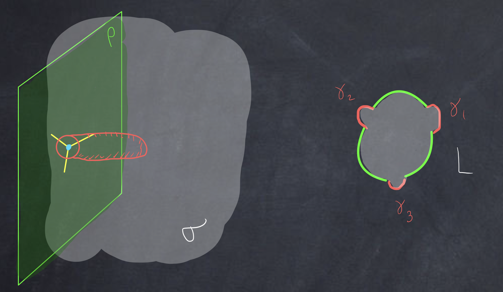
Figure 33. A defect supported on a stratified submanifold and its link $L$

As a further example, consider a $\rho$-defect whose support is a graph, as depicted in Figure 33. This is a special case of the defect in Figure 29. The three line defects are labeled by an object in the category $\mathcal{L}$. We must supply a label for the point defect at the intersection of the line defects. Let $L$ be the link of the point. Observe that some portions of $\partial L$ are $\rho$-colored. By restriction we obtain a map

(4.15) $$\operatorname{Map}(L,\mathscr{X})\longrightarrow\Omega\mathscr{X}\times\Omega\mathscr{X}\times\Omega\mathscr{X}$$

The image consists of triples $(\gamma_{1},\gamma_{2},\gamma_{3})$ of based loops in $\mathscr{X}$ whose product $\gamma_{1}\gamma_{2}\gamma_{3}$ is null homotopic; the fiber over such a triple consists of null homotopies which, up to homotopy, form an $A$-torsor, since $\pi_{2}\mathscr{X}=A$. Therefore, in the quantization we expect that for fixed labels on the line defects, the possible labels on the point defect form a $\operatorname{Fun}(A)$-module. Indeed, if the lines are labeled by objects $\ell_{1},\ell_{2},\ell_{3}\in\mathcal{L}$, then $\ell_{1}*\ell_{2}*\ell_{3}$ must be isomorphic to $1$. The label on the point defect is a vector in $\operatorname{Hom}_{\mathcal{L}}(1,\ell_{1}*\ell_{2}*\ell_{3})$, and as expected this vector space is a module over $\operatorname{Hom}_{\mathcal{L}}(1,1)=\operatorname{Fun}(A)$.

4.4.2. An example with higher homotopy groups

Let $\mathscr{X}$ be the $\pi$-finite space whose Postnikov tower is

(4.16) $$B^{3}{\mathbb{Z}}/2{\mathbb{Z}}\longrightarrow\mathscr{X}\longrightarrow B^{2}{\mathbb{Z}}/2{\mathbb{Z}}$$

with $k$-invariant $\operatorname{Sq}^{2}\colon B^{2}{\mathbb{Z}}/2{\mathbb{Z}}\longrightarrow B^{4}{\mathbb{Z}}/2{\mathbb{Z}}$. Since the Steenrod square is a stable cohomology operation, $\mathscr{X}$ is an infinite loop space. We grade so that it is the 2-space in a spectrum $h$ which is an extension

(4.17) $$\Sigma H{\mathbb{Z}}/2{\mathbb{Z}}\xrightarrow{\;\;i\;\;}h\xrightarrow{\;\;j\;\;}H{\mathbb{Z}}/2{\mathbb{Z}}$$

The spectrum $h$ is similar to the spectrum $e$ in [F2, Proposition 4.4] with which it shares the following properties:

1. $h$ is a module over $ko$, the connective real $K$-theory spectrum,

2. $h$ is oriented for spin bundles, and

3. for any space $Z$ there is a natural identification of $h^{0}(Z)$ with the group of isomorphism classes of ${\mathbb{Z}}/2{\mathbb{Z}}$-graded double covers of $Z$.

We will exploit these properties to facilitate some computations.

Fix a positive integer $n$ and let $\sigma=\sigma_{\mathscr{X}}^{(n+1)}$ be the indicated finite homotopy theory. We emphasize that $\sigma$ is an unoriented theory, that is, there are no nontrivial background fields. Below we use a spin structure to derive some formulas for the quantum invariants, but the spin structure is not necessary to define the theory. Fix a basepoint of $\mathscr{X}$ to construct a regular boundary theory $\rho$. Let $X$ be an $n$-manifold and consider $\sigma$ on $[0,1)\times X$ with $\rho$-colored boundary at $\{0\}\times X$. We consider $\rho$-defects in this theory.

Codimension two defects: semiclassical and quantum

Let $Z\subset X$ be a codimension 2 submanifold with normal bundle $\pi\colon\nu\to Z$.

1. Semiclassical local defects. The link of $\{0\}\times Z\subset[0,1)\times X$ at $p\in Z$ can be identified with the unit disk $D(\nu_{p})$ in the fiber of the normal bundle. As in §4.4.1, the mapping space of semiclassical local defects is the space of pointed maps $D(\nu_{p})\!\bigm{/}\!\partial D(\nu_{p})\to\mathscr{X}$. A framing ${\mathbb{R}}^{2}\xrightarrow{\;\cong\;}\nu_{p}$ identifies this mapping space as

(4.18) $$\Omega^{2}\mathscr{X}\simeq{\mathbb{Z}}/2{\mathbb{Z}}\times B{\mathbb{Z}}/2{\mathbb{Z}}.$$

2. Automorphisms. The space of oriented framings ${\mathbb{R}}^{2}\xrightarrow{\;\cong\;}\nu_{p}$ is homotopy equivalent to a circle. Over that circle we have two fiber bundles and an isomorphism between them. One has fiber the space of pointed maps $D(\nu_{p})\!\bigm{/}\!\partial D(\nu_{p})\to\mathscr{X}$, and the other has fiber the space of pointed maps $D({\mathbb{R}}^{2})\!\bigm{/}\!\partial D({\mathbb{R}}^{2})\to\mathscr{X}$. The monodromy of the isomorphism between them is an automorphism of the identity of (4.18). On the component labeled by $0\in{\mathbb{Z}}/2{\mathbb{Z}}$ it is the identity automorphism. On the component labeled by $1\in{\mathbb{Z}}/2{\mathbb{Z}}$ it is the nontrivial automorphism of the identity functor of $B{\mathbb{Z}}/2{\mathbb{Z}}$.

3. Semiclassical global defects. Globally over $Z$, consider the space $\operatorname{Map}(Z^{\nu},\mathscr{X})$ of pointed maps out of the Thom space $Z^{\nu}$ of the normal bundle. Assume that the normal bundle admits a spin structure. Homotopy classes of maps $Z^{\nu}\to\mathscr{X}$ form the cohomology group $h^{2}(Z^{\nu})$, and the existence of the spin structure on the normal bundle implies that $h^{2}(Z^{\nu})$ sits in an exact sequence (compare (4.21) below)

(4.19) $$0\longrightarrow H^{1}(Z;{\mathbb{Z}}/2{\mathbb{Z}})\longrightarrow h^{2}(Z^{\nu})\longrightarrow H^{0}(Z;{\mathbb{Z}}/2{\mathbb{Z}})\longrightarrow 0,$$

where we have used the Thom isomorphism in cohomology with ${\mathbb{Z}}/2{\mathbb{Z}}$ coefficients. The composition law on defects is the standard abelian group structure on $h^{2}(Z^{\nu})$.

4. Splitting the sequence. Now choose a spin structure on the normal bundle $\pi\colon\nu\to Z$. Then the Thom isomorphism for the cohomology theory $h$ identifies $h^{2}(Z^{\nu})$ as the abelian group $h^{0}(Z)$, which is isomorphic to a direct product of the quotient and sub in (4.19). Its elements are pairs $(g,\rho)$ consisting of a locally constant function $g\colon Z\to{\mathbb{Z}}/2{\mathbb{Z}}$ and a double cover $\rho\colon\widetilde{Z}\to Z$. Now shift the spin structure on $\pi\colon\nu\to Z$ by a double cover of $Z$. It follows from essentially the same argument as in [F2, Proposition 4.4] that the shift in the Thom isomorphism $h^{2}(Z^{\nu})\xrightarrow{\;\cong\;}h^{0}(Z)$ is the shearing

(4.20) $$(g,\rho)\mapsto(g,\rho+g\delta)$$

on $h^{0}(Z)$, where $\delta\in H^{1}(Z;{\mathbb{Z}}/2{\mathbb{Z}})$ classifies the difference of spin structures.

5. Dehn twists. This dependence on spin structures can be manifested as follows. Cut $Z$ along a codimension one hypersurface Poincaré dual to $\delta\in H^{1}(Z;{\mathbb{Z}}/2{\mathbb{Z}})$ and reglue using a full twist on the link. This gives a “Dehn twist” automorphism of $Z^{\nu}$. It shifts the spin structure by $\delta$, and so it acts on the space of global labels by the shearing (4.20).

6. The $w_{2}$ obstruction. Dropping the assumption that the normal bundle $\pi$ has a spin structure, (4.19) is replaced by the exact sequence

(4.21) $$0\longrightarrow H^{1}(Z;{\mathbb{Z}}/2{\mathbb{Z}})\longrightarrow h^{2}(Z^{\nu})\longrightarrow H^{0}(Z;{\mathbb{Z}}/2{\mathbb{Z}})\xrightarrow{\;\;w_{2}(\nu)\;\;}H^{2}(Z;{\mathbb{Z}}/2{\mathbb{Z}}).$$

Hence the group $h^{2}(Z^{\nu})$ of isomorphism classes of defects does not allow a nonzero $H^{0}$ “part” on components of $Z$ over which the normal bundle is not spinable.

The link of a codimension 2 defect is a circle, and the value of any topological field theory on a circle has an $E_{2}$-structure. Semiclassically, that $E_{2}$-structure on the double loop space $\Omega^{2}\mathscr{X}$ in (4.18) recovers the space $\mathscr{X}$.

This concludes the semiclassical discussion.

7. Local quantum defects. For definiteness take $n=3$. Then the quantization of (4.18) is the linear category of ${\mathbb{Z}}/2{\mathbb{Z}}$-graded representations of ${\mathbb{Z}}/2{\mathbb{Z}}$. As an $E_{2}$-category, i.e., a braided tensor category, this is $\operatorname{Vect}\langle{\mathbb{Z}}/2{\mathbb{Z}}\rangle\oplus s\!\operatorname{Vect}$, the sum of the braided tensor categories of ${\mathbb{Z}}/2{\mathbb{Z}}$-graded vector spaces and super vector spaces. This comes about as the Karoubi completion of the span of two objects ($\pi_{2}\mathscr{X}$), each with endomorphism algebra ${\mathbb{C}}[\pi_{3}\mathscr{X}]={\mathbb{C}}[{\mathbb{Z}}/2{\mathbb{Z}}]$. This is the linear category of local topological line $\rho$-defects.

As tensor categories, $\operatorname{Vect}\langle{\mathbb{Z}}/2{\mathbb{Z}}\rangle$ is equivalent to $s\!\operatorname{Vect}$. However, the braiding is different due to the Koszul sign rule in the latter. It is induced from the $k$-invariant between $\pi_{2}\mathscr{X}$ and $\pi_{3}\mathscr{X}$ and is the action of the nonidentity element in the latter group. Said differently, the identification in (4.18) preserves the group structure but not the commutativity at the $E_{2}$ level. This manifests in the braiding of global line defects in the 3-manifold $X$.

8. Global quantum defects. The global quantum defects supported on $Z\subset X$ form the vector space of functions on $h^{2}(Z^{\nu})$; see point (3) above. The integration of local quantum defects to global quantum defects assigns a vector in this vector space to each object in the category $\operatorname{Vect}\langle{\mathbb{Z}}/2{\mathbb{Z}}\rangle\oplus s\!\operatorname{Vect}$. This map depends on a trivialization of $\nu\to Z$; a change of trivialization acts by the shearing (4.20).

If $Z^{\prime}$ is a parallel copy of $Z$, then we can identify the vector spaces of global defects on $Z$ and $Z^{\prime}$ and define a composition law; see Section 2.4. In this case the result is the group algebra ${\mathbb{C}}[h^{2}(Z^{\nu})]$.

Codimension one defects

We now undertake an analogous study of codimension one defects.

1. Semiclassical global defects. Consider a codimension 1 submanifold $W\subset X$. Then the analog of (4.21) is the exact sequence

(4.22) $$0\longrightarrow H^{2}(W;{\mathbb{Z}}/2{\mathbb{Z}})\longrightarrow h^{2}(W^{\nu})\longrightarrow H^{1}(W;{\mathbb{Z}}/2{\mathbb{Z}})\xrightarrow{\;\;w_{1}(\nu)\,\smile\,\operatorname{Sq}^{1}\;\;}H^{3}(W;{\mathbb{Z}}/2{\mathbb{Z}})$$

Assume the normal bundle $\nu\to W$ to $W\subset X$ is trivialized. As before, a choice of spin structure on $\nu\to W$ induces a Thom isomorphism on $h^{\bullet}$ and a splitting

(4.23) $$h^{2}(W^{\nu})\cong h^{1}(W)\cong H^{1}(W;{\mathbb{Z}}/2{\mathbb{Z}})\oplus H^{2}(W;{\mathbb{Z}}/2{\mathbb{Z}}).$$

Different spin structures shear the splitting, as in (4.20). However, (4.23)  is only an isomorphism of sets, not of abelian groups. The nonzero $k$-invariant $\operatorname{Sq}^{2}$ in (4.16) implies that the abelian group law on $h^{2}(W^{\nu})$ transports to the group law

(4.24) $$(a_{1},b_{1})+(a_{2},b_{2})=(a_{1}+a_{2},b_{1}+b_{2}+a_{1}\smile a_{2})$$

on $H^{1}(W;{\mathbb{Z}}/2{\mathbb{Z}})\oplus H^{2}(W;{\mathbb{Z}}/2{\mathbb{Z}})$.

2. Composition law. One consequence of the group law (4.24) is that the square of a defect whose class in (4.23) is $(a,0)$ has equivalence class $(0,a\smile a)$. In particular, such a defect need not be of order two.

When the normal bundle $\nu\to W$ is not trivial we can still have a self composition law of double covering defects of $W$. Let $\widetilde{W}$ be the boundary of a tubular neighborhood of $W$, and denote by $p\colon\widetilde{W}\to W$ the double cover. Write $\delta=w_{1}(\nu)\in H^{1}(W;{\mathbb{Z}}/2{\mathbb{Z}})$. Consider the following process: begin with a defect supported on $W$, pull back to a defect supported on $\widetilde{W}$, and then compose the defects on the two sheets to obtain a defect supported on $W$. On isomorphism classes of defects this process induces the map

(4.25) $$p_{*}\circ p^{*}\colon h^{2}(W^{\nu})\longrightarrow h^{2}(W^{\nu})$$

The map $p_{*}\circ p^{*}$ on ordinary cohomology is multiplication by the order of the cover, which is 2, and so it vanishes on mod 2 cohomology. Apply this twice to the short exact sequences (4.22) for $W$ and $\widetilde{W}$ to conclude: (1) the value of (4.25) on a class in $h^{2}(W^{\nu})$ only depends on its image in the quotient $H^{1}(W;{\mathbb{Z}}/2{\mathbb{Z}})$, and (2) the result lies in the subgroup $H^{2}(W;{\mathbb{Z}}/2{\mathbb{Z}})$. We claim that (4.25) is the restriction of the quadratic map

(4.26) $$H^{1}(W;{\mathbb{Z}}/2{\mathbb{Z}}) \longrightarrow H^{2}(W;{\mathbb{Z}}/2{\mathbb{Z}})$$

$$a \longmapsto\quad\;a^{2}+\delta a$$

to the subgroup of $H^{1}(W;{\mathbb{Z}}/2{\mathbb{Z}})$ cut out by the last map in (4.22). Namely, (4.25) is a natural quadratic map for all spaces $W$ equipped with a double cover, hence is a linear combination of $a^{2},\delta a,\delta^{2}$. Furthermore, it vanishes when $a=0$ or $a=\delta$, and it reduces to $a^{2}$ when $\delta=0$ by the previous paragraph. It follows that (4.26) is the only possibility.

3. Local quantum defects. Specialize to $n=3$. For local defects, we quantize $\Omega\mathscr{X}$ to a tensor category. Since $\Omega\mathscr{X}$ is a based loop space the tensor category has an additional $E_{1}$-structure. Proceeding as in point  (7) above for codimension two defects, we first quantize $\Omega^{2}\mathscr{X}$ as a linear category, use one loop to derive the tensor structure, and use the second loop to derive the $E_{1}$-structure. The result is a braided tensor category, namely the same braided tensor category $\operatorname{Vect}\langle{\mathbb{Z}}/2{\mathbb{Z}}\rangle\oplus s\!\operatorname{Vect}$ as in point  (7) above.

4. Global quantum defects. On $W\subset X$, the quantization of the semiclassical global defects of point (1) above is the vector space of functions on the group $h^{2}(W^{\nu})$ in (4.22). Integration of an unobstructed object in the category $\operatorname{Vect}\langle{\mathbb{Z}}/2{\mathbb{Z}}\rangle\oplus s\!\operatorname{Vect}$ gives a vector in this vector space, but the result depends on a choice of spin structure on the normal bundle.

If the normal bundle $\nu\to W$ is trivialized, then the composition of defects is encoded in an algebra structure on this vector space, namely the group algebra of the group law (4.24).

5. Quotient and duality defects

In this section we take up two types of defects which have been discussed in the literature recently: quotient defects and duality defects. Recall from §3.4 that the quotient $F\!\mkern-1.5mu\bigm{/}_{\!\mkern-1.5mu\epsilon}\!\sigma$ of a field theory $F$ by a symmetry $\sigma$ is defined using an augmentation. Now, in §5.1, we use an augmentation to define a defect on a positive codimensional submanifold which, in effect, takes the quotient on that submanifold. Returning to the quotient theory, there are special situations in which there exists an isomorphism $F\!\mkern-1.5mu\bigm{/}_{\!\mkern-1.5mu\epsilon}\!\sigma\to F$. In §5.2 we use such an isomorphism to define a self-domain wall of $F$ called a duality defect, and we give some applications.

5.1. Quotient defects: quotienting on a submanifold

Fix a positive integer $n$ and an $n$-dimensional quiche $(\sigma,\rho)$. Suppose $\epsilon$ is an augmentation of $\sigma$, as in Definition 3.4. As explained in Definition 3.4, if $(\widetilde{F},\theta)$ is a $(\sigma,\rho)$-module structure on an $n$-dimensional quantum field theory $F$, then dimensional reduction of $\sigma$ along the closed interval depicted in Figure 15, which is the sandwich $\epsilon\otimes_{\sigma}\widetilde{F}$, is the quotient $F\!\mkern-1.5mu\bigm{/}_{\!\mkern-1.5mu\epsilon}\!\sigma$ of $F$ by the symmetry. This can be interpreted as the theory $F$ with the topological space-filling defect $\epsilon$.

There is a generalization which places the defect on a submanifold; see [RSS] and the references therein. For this, recall the Dirichlet-to-Neumann and Neumann-to-Dirichlet domain walls $\delta,\delta^{*}$ introduced in Definition 3.4. Suppose $M$ is a bordism on which we evaluate $F$, and suppose $Z\subset M$ is a submanifold of codimension $\ell$ on which we place the defect. (We do not make background fields explicit here; see §2.5.) Form the sandwich $[0,1]\times M$ with $\{0\}\times M$ colored with $\rho$ and $\{1\}\times M$ colored with $\widetilde{F}$. Let $\nu\subset M$ be an open tubular neighborhood of $Z\subset M$ with projection $\pi\colon\nu\to Z$, and arrange that the closure $\bar{\nu}$ of $\nu$ is the total space of a disk bundle $\bar{\nu}\to Z$.

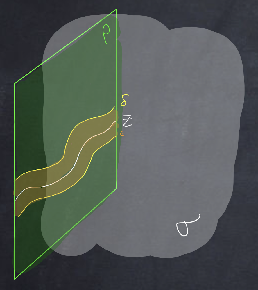
Figure 34. The quotient defect $\epsilon(Z)$

Definition .

The quotient defect $\epsilon(Z)$ is the $\rho$-defect supported on $\{0\}\times\bar{\nu}$ with $\{0\}\times\nu$ colored with $\epsilon$ and $\{0\}\times\partial\bar{\nu}$ colored with $\delta$.

This defect is depicted in Figure 34. The label $\delta$ is for the domain wall from $\rho$ to $\epsilon$; if we read in the other direction from $\epsilon$ to $\rho$, then the label is $\delta^{*}$.

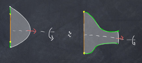
Figure 35. The local label of $\epsilon(Z)$ in codimension 1

Next, we compute the local label of the quotient defect $\epsilon(Z)$, as in Definition 2.4(1), and so express $\epsilon(Z)$ as a defect supported on $Z$. Consider a somewhat larger tubular neighborhood, now of $\{0\}\times Z\subset[0,1)\times M$. Recall $\ell=\operatorname{codim}^{\vphantom{1*\prime y\vee M}}_{\mkern-1.5muM}\!Z$. The tubular neighborhood for $\ell=1$ is depicted in Figure 35. Its value in the topological theory $\sigma$—with boundaries and defects $\rho,\epsilon,\delta$—is an object in $\operatorname{Hom}\bigl{(}1,\sigma(D^{1},S^{0}_{\delta})\bigr{)}$. (If $\mathscr{C}=\operatorname{Alg}(\mathscr{C}^{\prime})$ is the codomain of $\sigma$, and $\sigma(\operatorname{pt})=A$ is an algebra object in $\mathscr{C}^{\prime}$, then $\sigma(D^{1},S^{0}_{\delta})=A$ as an object of $\mathscr{C}^{\prime}$.)

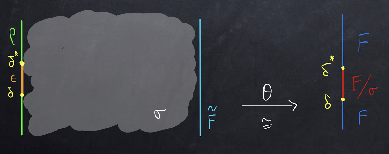
Figure 36. The codimension 1 quotient defect as a composition of domain walls

Remark .

The defect $\epsilon(Z)$ for $\ell=1$ can be interpreted as follows, assuming $Z\subset M$ has trivialized normal bundle. Let $Z_{1},Z_{2}$ be parallel normal translates of $Z$, color the region in between $\{0\}\times Z_{1}$ and $\{0\}\times Z_{2}$ with $\epsilon$, color the remainder of $\{0\}\times M$ with $\rho$, and use the domain wall $\delta$ at $\{0\}\times Z_{1}$ and $\{0\}\times Z_{2}$; see Figure 36. Then $\epsilon(Z)$ is the composition $\delta^{*}(Z_{2})*\delta(Z_{1})$. If a quantum field theory $F$ has a $(\sigma,\rho)$-module structure, then $\delta(Z_{1})$ is a domain wall from $F$ to $F\!\mkern-1.5mu\bigm{/}_{\!\mkern-1.5mu\epsilon}\!\sigma$ and $\delta^{*}(Z_{2})$ is a domain wall from $F\!\mkern-1.5mu\bigm{/}_{\!\mkern-1.5mu\epsilon}\!\sigma$ to $F$; the composition $\epsilon(Z)$ is a self domain wall of $F$.

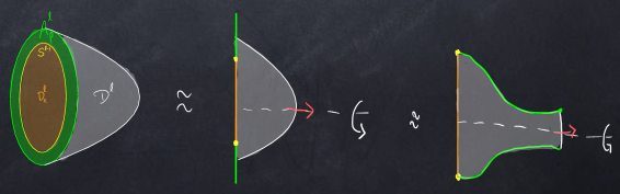
Figure 37. The local label of $\epsilon(Z)$ in codimension 2

The tubular neighborhood of $\{0\}\times Z\subset[0,1)\times M$ for codimension $\ell=2$ is the 3-dimensional bordism obtained from Figure 35 by revolution in 3-space, as illustrated in Figure 37. For general $\ell>1$, the bordism is the $(\ell+1)$-disk $D^{\ell+1}$ with boundary $S^{\ell}$ partitioned as

(5.1) $$\partial D^{\ell+1}=D^{\ell}_{\epsilon}\cup A^{\ell}_{\rho}\cup D^{\ell}$$

into a pair of disks $D^{\ell}$ and an annulus $A^{\ell}$; the domain wall $\delta$ is placed at the intersection of the $\epsilon$ and $\rho$-colored regions.

Remark .

These are the local defects. As always, the global defects are a section of a bundle (local system) of local defects over the submanifold $Z\subset M$.

Example (finite homotopy theory: local label).

Let $\sigma=\sigma_{\mathscr{X}}^{(n+1)}$ be the finite homotopy theory built from a $\pi$-finite space $\mathscr{X}$. Then we can use the calculus described in Appendix A to compute semiclassical spaces of defects. Suppose $\rho$ is specified by a basepoint $*\to\mathscr{X}$ and $\epsilon$ is specified by the identity map $\mathscr{X}\xrightarrow{\;\operatorname{id}\;}\mathscr{X}$. Then $\delta$, which is a domain wall between boundary theories (Section A.3.2), is specified by the homotopy fiber product

(5.2) $$\begin{gathered}\lx@xy@svg{\hbox{\raise 0.0pt\hbox{\kern 5.5pt\hbox{\ignorespaces\ignorespaces\ignorespaces\hbox{\vtop{\kern 0.0pt\offinterlineskip\halign{\entry@#!@&&\entry@@#!@\cr&\\&&\\&\crcr}}}\ignorespaces{\hbox{\kern-3.0pt\raise 0.0pt\hbox{\hbox{\kern 0.0pt\raise 0.0pt\hbox{\hbox{\kern 3.0pt\raise 0.0pt\hbox{$\textstyle{}$}}}}}}}{\hbox{\kern 30.75pt\raise 0.0pt\hbox{\hbox{\kern 0.0pt\raise 0.0pt\hbox{\hbox{\kern 3.0pt\raise 0.0pt\hbox{$\textstyle{\ast\ignorespaces\ignorespaces\ignorespaces\ignorespaces\ignorespaces\ignorespaces\ignorespaces\ignorespaces}$}}}}}}}\ignorespaces\ignorespaces\ignorespaces{}\ignorespaces\ignorespaces{\hbox{\lx@xy@drawline@}}\ignorespaces{\hbox{\kern 5.50002pt\raise-30.31824pt\hbox{\hbox{\kern 0.0pt\raise 0.0pt\hbox{\lx@xy@tip{1}\lx@xy@tip{-1}}}}}}\ignorespaces\ignorespaces{\hbox{\lx@xy@drawline@}}\ignorespaces{\hbox{\lx@xy@drawline@}}\ignorespaces\ignorespaces\ignorespaces{}\ignorespaces\ignorespaces{\hbox{\lx@xy@drawline@}}\ignorespaces{\hbox{\kern 67.0pt\raise-29.31604pt\hbox{\hbox{\kern 0.0pt\raise 0.0pt\hbox{\lx@xy@tip{1}\lx@xy@tip{-1}}}}}}\ignorespaces\ignorespaces{\hbox{\lx@xy@drawline@}}\ignorespaces{\hbox{\lx@xy@drawline@}}{\hbox{\kern-5.5pt\raise-35.74304pt\hbox{\hbox{\kern 0.0pt\raise 0.0pt\hbox{\hbox{\kern 3.0pt\raise 0.0pt\hbox{$\textstyle{\ast\ignorespaces\ignorespaces\ignorespaces\ignorespaces}$}}}}}}}\ignorespaces\ignorespaces\ignorespaces{}\ignorespaces\ignorespaces{\hbox{\lx@xy@drawline@}}\ignorespaces{\hbox{\kern 29.5pt\raise-65.72748pt\hbox{\hbox{\kern 0.0pt\raise 0.0pt\hbox{\lx@xy@tip{1}\lx@xy@tip{-1}}}}}}\ignorespaces\ignorespaces{\hbox{\lx@xy@drawline@}}\ignorespaces{\hbox{\lx@xy@drawline@}}{\hbox{\kern 33.25pt\raise-35.74304pt\hbox{\hbox{\kern 0.0pt\raise 0.0pt\hbox{\hbox{\kern 3.0pt\raise 0.0pt\hbox{$\textstyle{}$}}}}}}}{\hbox{\kern 67.0pt\raise-35.74304pt\hbox{\hbox{\kern 0.0pt\raise 0.0pt\hbox{\hbox{\kern 3.0pt\raise 0.0pt\hbox{$\textstyle{\mathscr{X}\ignorespaces\ignorespaces\ignorespaces\ignorespaces}$}}}}}}}\ignorespaces\ignorespaces\ignorespaces{}\ignorespaces\ignorespaces{\hbox{\lx@xy@drawline@}}\ignorespaces\ignorespaces\ignorespaces{\hbox{\kern 55.73628pt\raise-58.76105pt\hbox{{}\hbox{\kern 0.0pt\raise 0.0pt\hbox{\hbox{\kern 3.0pt\hbox{\hbox{\kern 0.0pt\raise-2.43056pt\hbox{$\scriptstyle{\operatorname{id}}$}}}\kern 3.0pt}}}}}}\ignorespaces{\hbox{\kern 43.00002pt\raise-65.945pt\hbox{\hbox{\kern 0.0pt\raise 0.0pt\hbox{\lx@xy@tip{1}\lx@xy@tip{-1}}}}}}\ignorespaces\ignorespaces{\hbox{\lx@xy@drawline@}}\ignorespaces{\hbox{\lx@xy@drawline@}}{\hbox{\kern-3.0pt\raise-72.57635pt\hbox{\hbox{\kern 0.0pt\raise 0.0pt\hbox{\hbox{\kern 3.0pt\raise 0.0pt\hbox{$\textstyle{}$}}}}}}}{\hbox{\kern 29.5pt\raise-72.57635pt\hbox{\hbox{\kern 0.0pt\raise 0.0pt\hbox{\hbox{\kern 3.0pt\raise 0.0pt\hbox{$\textstyle{\mathscr{X}}$}}}}}}}\ignorespaces}}}}\ignorespaces\end{gathered} \textstyle{\ast\ignorespaces\ignorespaces\ignorespaces\ignorespaces\ignorespaces\ignorespaces\ignorespaces\ignorespaces} \textstyle{\ast\ignorespaces\ignorespaces\ignorespaces\ignorespaces} \textstyle{\mathscr{X}\ignorespaces\ignorespaces\ignorespaces\ignorespaces} \scriptstyle{\operatorname{id}} \textstyle{\mathscr{X}} \textstyle{\ast\ignorespaces\ignorespaces\ignorespaces\ignorespaces\ignorespaces\ignorespaces\ignorespaces\ignorespaces} \textstyle{\ast\ignorespaces\ignorespaces\ignorespaces\ignorespaces} \textstyle{\mathscr{X}\ignorespaces\ignorespaces\ignorespaces\ignorespaces} \scriptstyle{\operatorname{id}} \textstyle{\mathscr{X}}$$

That the homotopy fiber product is a point $*$ is the manifestation of the uniqueness of $\delta$.

The space of maps from the link of a point of $Z$ into $\mathscr{X}$ is

(5.3) $$\operatorname{Map}\bigl{(}(D^{\ell},S^{\ell-1}),(\mathscr{X},*)\bigr{)}=\Omega^{\ell}\mathscr{X}.$$

Set

(5.4) $$N^{\ell}=\bigl{(}D^{\ell+1},A^{\ell}\bigr{)},$$

where $A^{\ell}\subset\partial D^{\ell+1}$; see (5.1) and Figure 37. The semiclassical local defect $\epsilon(Z)$, in the sense of Section A.3, is the map induced by restriction to $\Omega^{\ell}\mathscr{X}$:

(5.5) $$\operatorname{Map}(N^{\ell},\mathscr{X})\longrightarrow\Omega^{\ell}\mathscr{X}.$$

Here the basepoint in $\mathscr{X}$ is implicit. This map is a homotopy equivalence, as can be proved using the technique in [H, Example 0.8]. So we can replace (5.5) with the identity map on $\Omega^{\ell}\mathscr{X}$.

Now the map $\operatorname{id}\colon\Omega^{\ell}\mathscr{X}\to\Omega^{\ell}\mathscr{X}$, viewed as a correspondence from a point $*$ to $\Omega^{\ell}\mathscr{X}$, quantizes to an object in the quantization of $\Omega^{\ell}\mathscr{X}$, and it is typically noninvertible. For example, if we are at the level in which the quantization of $\Omega^{\ell}\mathscr{X}$ is a vector space, then the vector space is $\operatorname{Fun}(\pi_{0}\Omega^{\ell}\mathscr{X})=\operatorname{Fun}(\pi_{\ell}\mathscr{X})$, which typically has dimension $>1$. The local label we compute is the constant function 1. If the quantization is a linear category, then it is the category $\operatorname{Vect}(\Omega^{\ell}\mathscr{X})$ of flat vector bundles over $\Omega^{\ell}\mathscr{X}$, i.e., vector bundles on the fundamental groupoid $\pi_{\leq 1}\Omega^{\ell}\mathscr{X}$, and the local label is the trivial bundle with fiber ${\mathbb{C}}$.

Example (finite homotopy theory: global label).

We continue with Section 5.1, but now compute the global label of the defect $\epsilon(Z)$. As in §4.4.2, we must quantize

(5.6) $$\operatorname{id}\colon\operatorname{Map}(Z^{\nu},\mathscr{X})\longrightarrow\operatorname{Map}(Z^{\nu},\mathscr{X}),$$

where $Z^{\nu}$ is the Thom space of the normal bundle. As an example, suppose $\ell=1$ and assume that the normal bundle $\nu\to Z$ has been trivialized. (This amounts to a coorientation of the codimension 1 submanifold $Z\subset M$—a direction for the domain wall.) Then

(5.7) $$\operatorname{Map}(Z^{\nu},\mathscr{X})\simeq\operatorname{Map}(Z,\Omega\mathscr{X}).$$

For example, if $A$ is a finite abelian group and $\mathscr{X}=B^{2}\!A$—so $\sigma$ encodes a $BA$-symmetry—then $\operatorname{Map}(Z^{\nu},B^{2}\!A)\simeq\operatorname{Map}(Z,BA)$ is the “space” of principal $A$-bundles $P\to Z$. One should, rather, treat it as a groupoid, the groupoid $\operatorname{Bun}_{A}(Z)$ of principal $A$-bundles over $Z$ and isomorphisms between them. A point $*\to\operatorname{Bun}_{A}(Z)$ is a principal $A$-bundle $P\to Z$, and this map quantizes to a global defect $\eta(P)$ supported on $Z$. The quantization of $\operatorname{id}\colon\operatorname{Bun}_{A}(Z)\to\operatorname{Bun}_{A}(Z)$ is a sum of the quantizations of $*\!\!\bigm{/}\!\!\operatorname{Aut}P\to\operatorname{Bun}_{A}(Z)$ over isomorphism classes of principal $A$-bundles $P\to Z$. Informally, we might write this as a sum over isomorphism classes of $P\to Z$ of

(5.8) $$\frac{1}{\#\operatorname{Aut}P}\,\eta(P)=\frac{1}{\#H^{0}(Z;A)}\,\eta(P).$$

This sort of expression appears in [CCHLS, (1.3)], for example.

The $\rho$-defect $\eta(P)$ has a geometric semiclassical interpretation. Without the defect one is summing over $A$-gerbes on $[0,1)\times M$ which are trivialized on $\{0\}\times M$. Putting the defect $\eta(P)$ on $\{0\}\times Z$ amounts to the instruction to trivialize the $A$-gerbe only on $\bigl{(}\{0\}\times M\bigr{)}\;\setminus\;\bigl{(}\{0\}\times Z\bigr{)}$ and to demand—relative to the coorientation of $Z$—that the trivialization jump by the $A$-bundle $P\to Z$. (Compare Remark 4.2(1).)

Remark .

1. As stated in Remark 5.1, the defect $\epsilon(Z)$ is the composition of the Dirichlet$\to$Neumann and Neumann$\to$Dirichlet domain walls in case $\ell=1$. In terms of $\pi$-finite spaces, that computation is the homotopy fiber product

   (5.9) $$\begin{gathered}\lx@xy@svg{\hbox{\raise 0.0pt\hbox{\kern 5.5pt\hbox{\ignorespaces\ignorespaces\ignorespaces\hbox{\vtop{\kern 0.0pt\offinterlineskip\halign{\entry@#!@&&\entry@@#!@\cr&&\\&&&\\&&&&\\\\&&\crcr}}}\ignorespaces{\hbox{\kern-3.0pt\raise 0.0pt\hbox{\hbox{\kern 0.0pt\raise 0.0pt\hbox{\hbox{\kern 3.0pt\raise 0.0pt\hbox{$\textstyle{}$}}}}}}}{\hbox{\kern 26.0pt\raise 0.0pt\hbox{\hbox{\kern 0.0pt\raise 0.0pt\hbox{\hbox{\kern 3.0pt\raise 0.0pt\hbox{$\textstyle{}$}}}}}}}{\hbox{\kern 52.5pt\raise 0.0pt\hbox{\hbox{\kern 0.0pt\raise 0.0pt\hbox{\hbox{\kern 3.0pt\raise 0.0pt\hbox{$\textstyle{\Omega\mathscr{X}\ignorespaces\ignorespaces\ignorespaces\ignorespaces\ignorespaces\ignorespaces\ignorespaces\ignorespaces}$}}}}}}}\ignorespaces\ignorespaces\ignorespaces{}\ignorespaces\ignorespaces{\hbox{\lx@xy@drawline@}}\ignorespaces{\hbox{\kern 34.50002pt\raise-24.91443pt\hbox{\hbox{\kern 0.0pt\raise 0.0pt\hbox{\lx@xy@tip{1}\lx@xy@tip{-1}}}}}}\ignorespaces\ignorespaces{\hbox{\lx@xy@drawline@}}\ignorespaces{\hbox{\lx@xy@drawline@}}\ignorespaces\ignorespaces\ignorespaces{}\ignorespaces\ignorespaces{\hbox{\lx@xy@drawline@}}\ignorespaces{\hbox{\kern 91.22223pt\raise-24.9198pt\hbox{\hbox{\kern 0.0pt\raise 0.0pt\hbox{\lx@xy@tip{1}\lx@xy@tip{-1}}}}}}\ignorespaces\ignorespaces{\hbox{\lx@xy@drawline@}}\ignorespaces{\hbox{\lx@xy@drawline@}}{\hbox{\kern-3.0pt\raise-29.74304pt\hbox{\hbox{\kern 0.0pt\raise 0.0pt\hbox{\hbox{\kern 3.0pt\raise 0.0pt\hbox{$\textstyle{}$}}}}}}}{\hbox{\kern 23.5pt\raise-29.74304pt\hbox{\hbox{\kern 0.0pt\raise 0.0pt\hbox{\hbox{\kern 3.0pt\raise 0.0pt\hbox{$\textstyle{\ast\ignorespaces\ignorespaces\ignorespaces\ignorespaces\ignorespaces\ignorespaces\ignorespaces\ignorespaces}$}}}}}}}\ignorespaces\ignorespaces\ignorespaces{}\ignorespaces\ignorespaces{\hbox{\lx@xy@drawline@}}\ignorespaces{\hbox{\kern 5.50002pt\raise-53.84642pt\hbox{\hbox{\kern 0.0pt\raise 0.0pt\hbox{\lx@xy@tip{1}\lx@xy@tip{-1}}}}}}\ignorespaces\ignorespaces{\hbox{\lx@xy@drawline@}}\ignorespaces{\hbox{\lx@xy@drawline@}}\ignorespaces\ignorespaces\ignorespaces{}\ignorespaces\ignorespaces{\hbox{\lx@xy@drawline@}}\ignorespaces{\hbox{\kern 56.11111pt\raise-53.56665pt\hbox{\hbox{\kern 0.0pt\raise 0.0pt\hbox{\lx@xy@tip{1}\lx@xy@tip{-1}}}}}}\ignorespaces\ignorespaces{\hbox{\lx@xy@drawline@}}\ignorespaces{\hbox{\lx@xy@drawline@}}{\hbox{\kern 59.86111pt\raise-29.74304pt\hbox{\hbox{\kern 0.0pt\raise 0.0pt\hbox{\hbox{\kern 3.0pt\raise 0.0pt\hbox{$\textstyle{}$}}}}}}}{\hbox{\kern 91.22223pt\raise-29.74304pt\hbox{\hbox{\kern 0.0pt\raise 0.0pt\hbox{\hbox{\kern 3.0pt\raise 0.0pt\hbox{$\textstyle{\ast\ignorespaces\ignorespaces\ignorespaces\ignorespaces\ignorespaces\ignorespaces\ignorespaces\ignorespaces}$}}}}}}}\ignorespaces\ignorespaces\ignorespaces{}\ignorespaces\ignorespaces{\hbox{\lx@xy@drawline@}}\ignorespaces{\hbox{\kern 69.61113pt\raise-53.56006pt\hbox{\hbox{\kern 0.0pt\raise 0.0pt\hbox{\lx@xy@tip{1}\lx@xy@tip{-1}}}}}}\ignorespaces\ignorespaces{\hbox{\lx@xy@drawline@}}\ignorespaces{\hbox{\lx@xy@drawline@}}\ignorespaces\ignorespaces\ignorespaces{}\ignorespaces\ignorespaces{\hbox{\lx@xy@drawline@}}\ignorespaces{\hbox{\kern 120.22223pt\raise-53.8518pt\hbox{\hbox{\kern 0.0pt\raise 0.0pt\hbox{\lx@xy@tip{1}\lx@xy@tip{-1}}}}}}\ignorespaces\ignorespaces{\hbox{\lx@xy@drawline@}}\ignorespaces{\hbox{\lx@xy@drawline@}}{\hbox{\kern-5.5pt\raise-59.48608pt\hbox{\hbox{\kern 0.0pt\raise 0.0pt\hbox{\hbox{\kern 3.0pt\raise 0.0pt\hbox{$\textstyle{\ast\ignorespaces\ignorespaces\ignorespaces\ignorespaces}$}}}}}}}\ignorespaces\ignorespaces\ignorespaces{}\ignorespaces\ignorespaces{\hbox{\lx@xy@drawline@}}\ignorespaces{\hbox{\kern 56.11111pt\raise-108.43951pt\hbox{\hbox{\kern 0.0pt\raise 0.0pt\hbox{\lx@xy@tip{1}\lx@xy@tip{-1}}}}}}\ignorespaces\ignorespaces{\hbox{\lx@xy@drawline@}}\ignorespaces{\hbox{\lx@xy@drawline@}}{\hbox{\kern 26.0pt\raise-59.48608pt\hbox{\hbox{\kern 0.0pt\raise 0.0pt\hbox{\hbox{\kern 3.0pt\raise 0.0pt\hbox{$\textstyle{}$}}}}}}}{\hbox{\kern 56.11111pt\raise-59.48608pt\hbox{\hbox{\kern 0.0pt\raise 0.0pt\hbox{\hbox{\kern 3.0pt\raise 0.0pt\hbox{$\textstyle{\mathscr{X}\ignorespaces\ignorespaces\ignorespaces\ignorespaces}$}}}}}}}\ignorespaces\ignorespaces\ignorespaces\ignorespaces{}{\hbox{\lx@xy@droprule}}\ignorespaces{\hbox{\kern 62.86111pt\raise-104.48608pt\hbox{\hbox{\kern 0.0pt\raise 0.0pt\hbox{\lx@xy@tip{1}\lx@xy@tip{-1}}}}}}{\hbox{\lx@xy@droprule}}{\hbox{\lx@xy@droprule}}{\hbox{\kern 93.72223pt\raise-59.48608pt\hbox{\hbox{\kern 0.0pt\raise 0.0pt\hbox{\hbox{\kern 3.0pt\raise 0.0pt\hbox{$\textstyle{}$}}}}}}}{\hbox{\kern 120.22223pt\raise-59.48608pt\hbox{\hbox{\kern 0.0pt\raise 0.0pt\hbox{\hbox{\kern 3.0pt\raise 0.0pt\hbox{$\textstyle{\ast\ignorespaces\ignorespaces\ignorespaces\ignorespaces}$}}}}}}}\ignorespaces\ignorespaces\ignorespaces{}\ignorespaces\ignorespaces{\hbox{\lx@xy@drawline@}}\ignorespaces{\hbox{\kern 69.61113pt\raise-108.43292pt\hbox{\hbox{\kern 0.0pt\raise 0.0pt\hbox{\lx@xy@tip{1}\lx@xy@tip{-1}}}}}}\ignorespaces\ignorespaces{\hbox{\lx@xy@drawline@}}\ignorespaces{\hbox{\lx@xy@drawline@}}{\hbox{\kern-3.0pt\raise-86.90274pt\hbox{\hbox{\kern 0.0pt\raise 0.0pt\hbox{\hbox{\kern 3.0pt\raise 0.0pt\hbox{$\textstyle{}$}}}}}}}{\hbox{\kern-3.0pt\raise-114.3194pt\hbox{\hbox{\kern 0.0pt\raise 0.0pt\hbox{\hbox{\kern 3.0pt\raise 0.0pt\hbox{$\textstyle{}$}}}}}}}{\hbox{\kern 26.0pt\raise-114.3194pt\hbox{\hbox{\kern 0.0pt\raise 0.0pt\hbox{\hbox{\kern 3.0pt\raise 0.0pt\hbox{$\textstyle{}$}}}}}}}{\hbox{\kern 56.11111pt\raise-114.3194pt\hbox{\hbox{\kern 0.0pt\raise 0.0pt\hbox{\hbox{\kern 3.0pt\raise 0.0pt\hbox{$\textstyle{\mathscr{X}}$}}}}}}}\ignorespaces}}}}\ignorespaces\end{gathered} \textstyle{\Omega\mathscr{X}\ignorespaces\ignorespaces\ignorespaces\ignorespaces\ignorespaces\ignorespaces\ignorespaces\ignorespaces} \textstyle{\ast\ignorespaces\ignorespaces\ignorespaces\ignorespaces\ignorespaces\ignorespaces\ignorespaces\ignorespaces} \textstyle{\ast\ignorespaces\ignorespaces\ignorespaces\ignorespaces\ignorespaces\ignorespaces\ignorespaces\ignorespaces} \textstyle{\ast\ignorespaces\ignorespaces\ignorespaces\ignorespaces} \textstyle{\mathscr{X}\ignorespaces\ignorespaces\ignorespaces\ignorespaces} \textstyle{\ast\ignorespaces\ignorespaces\ignorespaces\ignorespaces} \textstyle{\mathscr{X}} \textstyle{\Omega\mathscr{X}\ignorespaces\ignorespaces\ignorespaces\ignorespaces\ignorespaces\ignorespaces\ignorespaces\ignorespaces} \textstyle{\ast\ignorespaces\ignorespaces\ignorespaces\ignorespaces\ignorespaces\ignorespaces\ignorespaces\ignorespaces} \textstyle{\ast\ignorespaces\ignorespaces\ignorespaces\ignorespaces\ignorespaces\ignorespaces\ignorespaces\ignorespaces} \textstyle{\ast\ignorespaces\ignorespaces\ignorespaces\ignorespaces} \textstyle{\mathscr{X}\ignorespaces\ignorespaces\ignorespaces\ignorespaces} \textstyle{\ast\ignorespaces\ignorespaces\ignorespaces\ignorespaces} \textstyle{\mathscr{X}}$$

   which is then the domain wall

   (5.10) $$\begin{gathered}\lx@xy@svg{\hbox{\raise 0.0pt\hbox{\kern 5.5pt\hbox{\ignorespaces\ignorespaces\ignorespaces\hbox{\vtop{\kern 0.0pt\offinterlineskip\halign{\entry@#!@&&\entry@@#!@\cr&\\&&\\&\crcr}}}\ignorespaces{\hbox{\kern-3.0pt\raise 0.0pt\hbox{\hbox{\kern 0.0pt\raise 0.0pt\hbox{\hbox{\kern 3.0pt\raise 0.0pt\hbox{$\textstyle{}$}}}}}}}{\hbox{\kern 29.5pt\raise 0.0pt\hbox{\hbox{\kern 0.0pt\raise 0.0pt\hbox{\hbox{\kern 3.0pt\raise 0.0pt\hbox{$\textstyle{\Omega\mathscr{X}\ignorespaces\ignorespaces\ignorespaces\ignorespaces\ignorespaces\ignorespaces\ignorespaces\ignorespaces}$}}}}}}}\ignorespaces\ignorespaces\ignorespaces{}\ignorespaces\ignorespaces{\hbox{\lx@xy@drawline@}}\ignorespaces{\hbox{\kern 5.50002pt\raise-30.81238pt\hbox{\hbox{\kern 0.0pt\raise 0.0pt\hbox{\lx@xy@tip{1}\lx@xy@tip{-1}}}}}}\ignorespaces\ignorespaces{\hbox{\lx@xy@drawline@}}\ignorespaces{\hbox{\lx@xy@drawline@}}\ignorespaces\ignorespaces\ignorespaces{}\ignorespaces\ignorespaces{\hbox{\lx@xy@drawline@}}\ignorespaces{\hbox{\kern 74.22223pt\raise-30.81775pt\hbox{\hbox{\kern 0.0pt\raise 0.0pt\hbox{\lx@xy@tip{1}\lx@xy@tip{-1}}}}}}\ignorespaces\ignorespaces{\hbox{\lx@xy@drawline@}}\ignorespaces{\hbox{\lx@xy@drawline@}}{\hbox{\kern-5.5pt\raise-35.74304pt\hbox{\hbox{\kern 0.0pt\raise 0.0pt\hbox{\hbox{\kern 3.0pt\raise 0.0pt\hbox{$\textstyle{\ast\ignorespaces\ignorespaces\ignorespaces\ignorespaces}$}}}}}}}\ignorespaces\ignorespaces\ignorespaces{}\ignorespaces\ignorespaces{\hbox{\lx@xy@drawline@}}\ignorespaces{\hbox{\kern 33.11111pt\raise-65.4414pt\hbox{\hbox{\kern 0.0pt\raise 0.0pt\hbox{\lx@xy@tip{1}\lx@xy@tip{-1}}}}}}\ignorespaces\ignorespaces{\hbox{\lx@xy@drawline@}}\ignorespaces{\hbox{\lx@xy@drawline@}}{\hbox{\kern 36.86111pt\raise-35.74304pt\hbox{\hbox{\kern 0.0pt\raise 0.0pt\hbox{\hbox{\kern 3.0pt\raise 0.0pt\hbox{$\textstyle{}$}}}}}}}{\hbox{\kern 74.22223pt\raise-35.74304pt\hbox{\hbox{\kern 0.0pt\raise 0.0pt\hbox{\hbox{\kern 3.0pt\raise 0.0pt\hbox{$\textstyle{\ast\ignorespaces\ignorespaces\ignorespaces\ignorespaces}$}}}}}}}\ignorespaces\ignorespaces\ignorespaces{}\ignorespaces\ignorespaces{\hbox{\lx@xy@drawline@}}\ignorespaces{\hbox{\kern 46.61113pt\raise-65.43481pt\hbox{\hbox{\kern 0.0pt\raise 0.0pt\hbox{\lx@xy@tip{1}\lx@xy@tip{-1}}}}}}\ignorespaces\ignorespaces{\hbox{\lx@xy@drawline@}}\ignorespaces{\hbox{\lx@xy@drawline@}}{\hbox{\kern-3.0pt\raise-71.48608pt\hbox{\hbox{\kern 0.0pt\raise 0.0pt\hbox{\hbox{\kern 3.0pt\raise 0.0pt\hbox{$\textstyle{}$}}}}}}}{\hbox{\kern 33.11111pt\raise-71.48608pt\hbox{\hbox{\kern 0.0pt\raise 0.0pt\hbox{\hbox{\kern 3.0pt\raise 0.0pt\hbox{$\textstyle{\mathscr{X}}$}}}}}}}\ignorespaces}}}}\ignorespaces\end{gathered} \textstyle{\Omega\mathscr{X}\ignorespaces\ignorespaces\ignorespaces\ignorespaces\ignorespaces\ignorespaces\ignorespaces\ignorespaces} \textstyle{\ast\ignorespaces\ignorespaces\ignorespaces\ignorespaces} \textstyle{\ast\ignorespaces\ignorespaces\ignorespaces\ignorespaces} \textstyle{\mathscr{X}} \textstyle{\Omega\mathscr{X}\ignorespaces\ignorespaces\ignorespaces\ignorespaces\ignorespaces\ignorespaces\ignorespaces\ignorespaces} \textstyle{\ast\ignorespaces\ignorespaces\ignorespaces\ignorespaces} \textstyle{\ast\ignorespaces\ignorespaces\ignorespaces\ignorespaces} \textstyle{\mathscr{X}}$$

   This recovers the description of $\epsilon(Z)$ in (5.5).

2. If the $\pi$-finite space $\mathscr{X}$ is equipped with a cocycle $\lambda$ which represents a cohomology class $[\lambda]\in h^{n}(\mathscr{X})$ for some cohomology theory $h$, then a codimension $\ell$ quotient defect has semiclassical label space $\Omega^{\ell}\mathscr{X}$ with transgressed cocycle and its cohomology class $[\tau^{\ell}\lambda]\in h^{n-\ell}(\Omega^{\ell}\mathscr{X})$. A nonzero cohomology class obstructs the quotient. However, as observed in [RSS] it is possible that $[\lambda]\neq 0$ but $[\tau^{\ell}\lambda]=0$ for some $\ell$, which means that the quotient by $\sigma$ does not exist but quotient defects of sufficiently high codimension do exist.

Example (Turaev-Viro symmetry).

Suppose $n=2$ and the 3-dimensional theory $\sigma$ is of Turaev-Viro type with $\sigma(\operatorname{pt})=\Phi$ a fusion category. Assume $\rho$ is given by the right regular module $\Phi_{\Phi}$ and $\epsilon$ is given by a fiber functor $\epsilon^{\vphantom{1*\prime y\vee M}}_{\Phi}\colon\Phi\to\operatorname{Vect}$. Then the codimension 1 quotient defect has local label the object $x_{\text{reg}}\in\Phi$ defined as

(5.11) $$x_{\text{reg}}=\sum\limits_{x}\epsilon^{\vphantom{1*\prime y\vee M}}_{\Phi}(x)^{*}\otimes x,$$

where the sum is over a representative set of simple objects $x$. See [FT1, Proposition 8.9] for a very similar computation.

5.2. Duality defects

This section is inspired by [CCHLS, KOZ]. Our approach separates out a topological sector of these quantum field theories and uses the calculus of defects we have developed.

Resume the general setup: $(\sigma,\rho)$ is an $n$-dimensional quiche, with $\rho$ a regular right $\sigma$-module, and $\sigma$ is equipped with an augmentation. Suppose $F$ is a quantum field theory equipped with a $(\sigma,\rho)$-module structure $(\sigma,\rho,\widetilde{F})$. Assume further that $F$ is equipped with an isomorphism

(5.12) $$\phi\colon F\!\mkern-1.5mu\bigm{/}_{\!\mkern-1.5mu\epsilon}\!\sigma\xrightarrow{\;\;\cong\;\;}F.$$

Example .

The existence of (5.12) is a special feature of $F$ and $\sigma$. An example with $n=2$ is the Ising model (for the group $\mbox{$\raisebox{-0.70007pt}{\rotatebox{9.9}{\tiny{\bf/} }}\mu\raisebox{-4.2194pt}{\scalebox{2.0}{$\color[rgb]{1,1,1}\phantom{.}$}}\raisebox{3.7889pt}{$\color[rgb]{1,1,1}\phantom{.}$}\hskip 4.60007pt$}_{2}$) at the critical temperature; see Example 3.5. In this case $\sigma$ is the 3-dimensional $\mbox{$\raisebox{-0.70007pt}{\rotatebox{9.9}{\tiny{\bf/} }}\mu\raisebox{-4.2194pt}{\scalebox{2.0}{$\color[rgb]{1,1,1}\phantom{.}$}}\raisebox{3.7889pt}{$\color[rgb]{1,1,1}\phantom{.}$}\hskip 4.60007pt$}_{2}$-gauge theory. For the five-state Potts model, also discussed in Example 3.5, $\sigma$ is the 3-dimensional $\mbox{$\raisebox{-0.70007pt}{\rotatebox{9.9}{\tiny{\bf/} }}\mu\raisebox{-4.2194pt}{\scalebox{2.0}{$\color[rgb]{1,1,1}\phantom{.}$}}\raisebox{3.7889pt}{$\color[rgb]{1,1,1}\phantom{.}$}\hskip 4.60007pt$}_{5}$-gauge theory. There are examples in $n=4$ discussed in [CCHLS, KOZ]. In these cases $\sigma$ is the 5-dimensional $\mbox{$\raisebox{-0.70007pt}{\rotatebox{9.9}{\tiny{\bf/} }}\mu\raisebox{-4.2194pt}{\scalebox{2.0}{$\color[rgb]{1,1,1}\phantom{.}$}}\raisebox{3.7889pt}{$\color[rgb]{1,1,1}\phantom{.}$}\hskip 4.60007pt$}_{2}$-gerbe theory $\sigma_{B^{2}\!\mbox{$\raisebox{-0.49005pt}{\rotatebox{9.9}{\tiny{\bf/} }}\mu\raisebox{-2.95358pt}{\scalebox{2.0}{$\color[rgb]{1,1,1}\phantom{.}$}}\raisebox{2.65222pt}{$\color[rgb]{1,1,1}\phantom{.}$}\hskip 3.22005pt$}_{2}}^{(5)}$. These include $\operatorname{U}_{1}$  Yang-Mills theory with coupling constant $\tau=2\sqrt{-1}$ and $N=4$ supersymmetric $\operatorname{SU}_{2}$ Yang-Mills theory with $\tau=\sqrt{-1}$.

Recall the domain walls $\delta\colon F\to F\!\mkern-1.5mu\bigm{/}_{\!\mkern-1.5mu\epsilon}\!\sigma$ and $\delta^{*}\colon F\!\mkern-1.5mu\bigm{/}_{\!\mkern-1.5mu\epsilon}\!\sigma\to F$ introduced in Definition 3.4.

Definition .

The duality defect is the self-domain wall

(5.13) $$\Delta=\phi\circ\delta\colon F\longrightarrow F.$$

Since $\delta$ is a topological defect, and $\phi$ is an isomorphism of theories, the composition $\Delta$ is also a topological defect.

View $\phi$ as a domain wall from $F$ to $F\!\mkern-1.5mu\bigm{/}_{\!\mkern-1.5mu\epsilon}\!\sigma$, and furthermore imagine that there is a 2-category of theories, domain walls, and domain walls between domain walls. Then we can consider the adjoint $\phi^{*}$. It is a general fact in 2-categories that if the 1-morphism  $\phi$ is invertible, then its adjoint equals its inverse: $\phi^{*}=\phi^{-1}$. Accepting all this, we compute

(5.14) $$\Delta^{*}\circ\Delta=(\phi\delta)^{*}(\phi\delta)=\delta^{*}\phi^{*}\phi\delta=\delta^{*}\phi^{-1}\phi\delta=\delta^{*}\circ\delta$$

The composition $\delta^{*}\circ\delta$ is the quotient defect; see Remark 5.1.

The following example illustrates a situation in which there is a larger quiche $(\hat{\sigma},\hat{\rho})$ in which we can interpret $\hat{\sigma}$ as $\sigma$ with $\Delta$ adjoined. In this situation $F$ has a $(\hat{\sigma},\hat{\rho})$-module structure. We do not attempt a general construction beyond the example.

Example .

In the case of the $n=2$ Ising model introduced in Example 5.2, the three dimensional $\mbox{$\raisebox{-0.70007pt}{\rotatebox{9.9}{\tiny{\bf/} }}\mu\raisebox{-4.2194pt}{\scalebox{2.0}{$\color[rgb]{1,1,1}\phantom{.}$}}\raisebox{3.7889pt}{$\color[rgb]{1,1,1}\phantom{.}$}\hskip 4.60007pt$}_{2}$-gauge theory $\sigma$ has $\sigma(\operatorname{pt})$ the fusion category whose set of isomorphism classes of simple objects is identified with $\mbox{$\raisebox{-0.70007pt}{\rotatebox{9.9}{\tiny{\bf/} }}\mu\raisebox{-4.2194pt}{\scalebox{2.0}{$\color[rgb]{1,1,1}\phantom{.}$}}\raisebox{3.7889pt}{$\color[rgb]{1,1,1}\phantom{.}$}\hskip 4.60007pt$}_{2}=\{1,\psi\}$. Then $\hat{\sigma}(\operatorname{pt})$ is the fusion category whose set of isomorphism classes of simple objects is $\{1,\psi,\Delta\}$, where the fusion rules are

(5.15) $$\psi^{2} =1$$

$$\psi\Delta =\Delta$$

$$\Delta^{2} =1+\psi$$

For the last equation, combine (5.14) with (5.7) or (5.11). This is an example of a Tambara–Yamagami fusion category [TY].

One can use this enhanced symmetry to draw dynamical conclusions. Namely, assume that $F$ is gapped and furthermore its infrared behavior is modeled by an invertible field theory $\lambda$. Furthermore, we posit that $\lambda$ carry a $(\sigma,\rho)$-module structure as well as a self-defect $\Delta$ which satisfies (5.14). (If we construct the larger symmetry $(\hat{\sigma},\hat{\rho})$, then we posit that $\lambda$ carry a $(\hat{\sigma},\hat{\rho})$-module structure.) Now because $\lambda$ is invertible, self-domain walls of $\lambda$ do not couple to $\lambda$; they are an independent field theories that act as an endomorphisms on $\lambda$. (Compare: an endomorphism of a line is multiplication by a complex number. More formally, since $\lambda$ is invertible, it follows that $\operatorname{End}(\lambda)\cong\operatorname{End}(\mathbbm{1})$.) So $\delta^{*}\circ\delta$ acts as multiplication by an $(n-1)$-dimensional topological field theory, and so too does $\Delta$ act as multiplication by a topological field theory. Those theories satisfy (5.14): $\Delta$ is a kind of square root of $\delta^{*}\circ\delta$. But in some situations no such square root exists, as we can prove using the well-developed principles of topological field theory. If so, this rules out the possibility of an invertible field theory in the infrared, i.e., the possibility that $F$ be “trivially gapped”. (We find the term ‘infrared invertible’ more suitable.)

Example .

Now take $\sigma=\sigma_{B^{2}\!\mbox{$\raisebox{-0.49005pt}{\rotatebox{9.9}{\tiny{\bf/} }}\mu\raisebox{-2.95358pt}{\scalebox{2.0}{$\color[rgb]{1,1,1}\phantom{.}$}}\raisebox{2.65222pt}{$\color[rgb]{1,1,1}\phantom{.}$}\hskip 3.22005pt$}_{2}}^{(5)}$ to be the $\mbox{$\raisebox{-0.70007pt}{\rotatebox{9.9}{\tiny{\bf/} }}\mu\raisebox{-4.2194pt}{\scalebox{2.0}{$\color[rgb]{1,1,1}\phantom{.}$}}\raisebox{3.7889pt}{$\color[rgb]{1,1,1}\phantom{.}$}\hskip 4.60007pt$}_{2}$-gerbe theory in 5 dimensions; it acts on 4-dimensional theories with $B\!\mbox{$\raisebox{-0.70007pt}{\rotatebox{9.9}{\tiny{\bf/} }}\mu\raisebox{-4.2194pt}{\scalebox{2.0}{$\color[rgb]{1,1,1}\phantom{.}$}}\raisebox{3.7889pt}{$\color[rgb]{1,1,1}\phantom{.}$}\hskip 4.60007pt$}_{2}$-symmetry. Assume that $\Delta$ is adjoined and that (5.14) is satisfied. The composition $\delta^{*}\circ\delta$ is computed in Remark 5.1(1); from (5.10) we see that it acts on an invertible 4-dimensional theory as multiplication by 3-dimensional $\mbox{$\raisebox{-0.70007pt}{\rotatebox{9.9}{\tiny{\bf/} }}\mu\raisebox{-4.2194pt}{\scalebox{2.0}{$\color[rgb]{1,1,1}\phantom{.}$}}\raisebox{3.7889pt}{$\color[rgb]{1,1,1}\phantom{.}$}\hskip 4.60007pt$}_{2}$-gauge theory $\Gamma=\sigma_{B\!\mbox{$\raisebox{-0.49005pt}{\rotatebox{9.9}{\tiny{\bf/} }}\mu\raisebox{-2.95358pt}{\scalebox{2.0}{$\color[rgb]{1,1,1}\phantom{.}$}}\raisebox{2.65222pt}{$\color[rgb]{1,1,1}\phantom{.}$}\hskip 3.22005pt$}_{2}}^{(3)}$.

Example .

Continue with Example 5.2. We claim there is no 3-dimensional topological field theory $T$ such that $T^{*}\circ T=\Gamma$. If so, evaluate on a point to obtain fusion categories $T(\operatorname{pt})$ and $\Gamma(\operatorname{pt})=\operatorname{Vect}[\mbox{$\raisebox{-0.70007pt}{\rotatebox{9.9}{\tiny{\bf/} }}\mu\raisebox{-4.2194pt}{\scalebox{2.0}{$\color[rgb]{1,1,1}\phantom{.}$}}\raisebox{3.7889pt}{$\color[rgb]{1,1,1}\phantom{.}$}\hskip 4.60007pt$}_{2}]$. The number of simple objects in $\operatorname{Vect}[\mbox{$\raisebox{-0.70007pt}{\rotatebox{9.9}{\tiny{\bf/} }}\mu\raisebox{-4.2194pt}{\scalebox{2.0}{$\color[rgb]{1,1,1}\phantom{.}$}}\raisebox{3.7889pt}{$\color[rgb]{1,1,1}\phantom{.}$}\hskip 4.60007pt$}_{2}]$ is 2, which is not a perfect square. The number of simple objects in $T^{*}(\operatorname{pt})\otimes T(\operatorname{pt})$ is a perfect square. This contradiction proves that there is no invertible left $\sigma$-module on which $\Delta$ acts.

Example .

One example is pure $U_{1}$-gauge theory $F$ in $n=4$ dimensions. Such a theory has a coupling constant $\tau$ which lies in the upper half plane. The quotient $F\!\mkern-1.5mu\bigm{/}_{\!\mkern-1.5mu\epsilon}\!\sigma$ by  $B\!\mbox{$\raisebox{-0.70007pt}{\rotatebox{9.9}{\tiny{\bf/} }}\mu\raisebox{-4.2194pt}{\scalebox{2.0}{$\color[rgb]{1,1,1}\phantom{.}$}}\raisebox{3.7889pt}{$\color[rgb]{1,1,1}\phantom{.}$}\hskip 4.60007pt$}_{2}$ is another $U_{1}$-gauge theory but with coupling constant $\tau/4$. The transformation $\tau\mapsto-1/\tau$ lifts to an isomorphism $\phi$ of the corresponding gauge theories. Hence for $\tau=2\sqrt{-1}$ the isomorphism $\phi$ maps as in (5.12). The previous arguments show that $F$ is not infrared invertible. (We know from other arguments that $F$ is not even gapped, much less infrared invertible.)

Another example with $B\!\mbox{$\raisebox{-0.70007pt}{\rotatebox{9.9}{\tiny{\bf/} }}\mu\raisebox{-4.2194pt}{\scalebox{2.0}{$\color[rgb]{1,1,1}\phantom{.}$}}\raisebox{3.7889pt}{$\color[rgb]{1,1,1}\phantom{.}$}\hskip 4.60007pt$}_{2}$-symmetry is $N=4$ supersymmetric $\operatorname{SU}_{2}$-gauge theory, which also has a coupling constant $\tau$. The quotient is $N=4$  supersymmetric $\operatorname{SO}_{3}$-gauge theory, and now S-duality can be used to supply the isomorphism $\phi$. (See [AST, §2.4] for a discussion of S-duality in these theories.) It turns out that one must take $\tau=\sqrt{-1}$. So we learn that this theory is not infrared invertible. (Again, it is not even gapped.)

Example .

Continue with the $n=2$ Ising model at the critical temperature (Example 5.2 and Example 5.2). In this case $\delta^{*}\circ\delta$  acts on an invertible 2-dimensional theory as multiplication by the 1-dimensional topological field theory which is the $\sigma$-model into $\mbox{$\raisebox{-0.70007pt}{\rotatebox{9.9}{\tiny{\bf/} }}\mu\raisebox{-4.2194pt}{\scalebox{2.0}{$\color[rgb]{1,1,1}\phantom{.}$}}\raisebox{3.7889pt}{$\color[rgb]{1,1,1}\phantom{.}$}\hskip 4.60007pt$}_{2}$; see Remark 5.1(1) or Example 5.1. In particular, the vector space attached to a point has dimension 2. Hence there is no square root: $\Delta$ acts as multiplication by a 1-dimensional topological field theory, as does $\Delta^{*}$, and the vector space attached to a point has the same dimension in both. Since $\sqrt{2}$ is not an integer, this cannot happen.

The Ising model at the critical temperature is not gapped, but the argument has more power applied instead to the five-state Potts model. There again the argument shows there cannot be a unique vacuum at the critical value of the parameter (the fixed point of the Kramers-Wannier involution of Example 3.5). Now, as opposed to in the previous examples, the theory is gapped at this critical parameter.

Remark .

In these examples the theory $F$ sits in a 1-parameter family $F_{s},\;s\in{\mathbb{R}}$, of theories in which the duality defect (5.13) extends to an involution $F_{s}\leftrightarrow F_{s^{*}}$ where $s\leftrightarrow s^{*}$ is an involution of the parameter space with unique fixed point $s_{c}$ and $F=F_{s_{c}}$. If we assume that $F_{s}$, $s\neq s_{c}$, is infrared invertible, and we also assume that there is a phase transition at  $s_{c}$, then we easily conclude that $F=F_{s_{c}}$ cannot be infrared invertible. (Either $F_{s_{c}}$ is gapless or if it is gapped the phase transition is of first-order and there is more than one vacuum.) But without the assumption that there is a phase transition, we cannot rule out the possibility that all $F_{s}$ are infrared invertible.

Appendix A Finite homotopy theories

The class of topological field theories described here was introduced by Kontsevich [Ko] in 1988 and was picked up by Quinn [Q] a few years later. They are also the subject of a series of papers by Turaev [Tu] in the early 2000’s. These finite homotopy theories lend themselves to explicit computation using topological techniques. Not only do they arise in examples, but they also form a useful playground for the general study of quantum field theory.

Quantization proceeds via finite algebraic processes, as opposed to the infinite dimensional analysis required for typical quantum field theories. The “finite path integral” quantization in fully local field theory was introduced in [F1] with further development in [FHLT, §3,§8]; see also [FT1, §9]. The modern approach uses ambidexterity or higher semiadditivity, as introduced by Hopkins–Lurie [HL]; see also [HeL, Ha, CSY, RS]. Nonetheless, as far as we know a definitive treatment is still missing. Here we summarize a bit about quantization of theories with an illustrative example. Then we indicate how to use mapping spaces to encode semiclassical defects, and how to quantize them via a finite path integral.

We can drop the $\pi$-finiteness assumption at the cost of only being able to carry out quantization below the top dimension; the sum which leads to a complex number is no longer finite and there is no topology to control convergence. Just below the top dimension we obtain functions on a possibly infinite discrete set, which is a well-defined vector space albeit not finite dimensional in general. Put differently, in the absence of $\pi$-finiteness we construct a once-categorified topological field theory (see Remark 2.1(1)).

A.1. $\pi$-finiteness

Definition .

1. A topological space $\mathscr{X}$ is $\pi$-finite if (i) $\pi_{0}\mathscr{X}$ is a finite set, (ii) for all $x\in\mathscr{X}$, the homotopy group $\pi_{q}(\mathscr{X},x)$, $q\geq 1$, is finite, and (iii) there exists $Q\in{\mathbb{Z}}^{>0}$ such that $\pi_{q}(\mathscr{X},x)=0$ for all $q>Q$, $x\in\mathscr{X}$. (For a fixed bound $Q$ we say that $\mathscr{X}$ is $Q$-finite.)

2. A continuous map $f\colon\mathscr{Y}\to\mathscr{Z}$ of topological spaces is $\pi$-finite if for all $z\in\mathscr{Z}$ the homotopy fiber over $z$ is a $\pi$-finite space.

3. A spectrum $E$ is $\pi$-finite if each space in the spectrum is a $\pi$-finite space.

Example .

An Eilenberg-MacLane space $K(\pi,q)$ is $\pi$-finite if $\pi$ is a finite group. We use notation which emphasizes the role of $\mathscr{X}$ as a classifying space: if $q=1$ we denote $K(\pi,1)$ by $B\pi$, and if $q\geq 1$ and $A$ is a finite abelian group, we denote $K(A,q)$ by $B^{q}\mkern-1.5muA$. In the text, for example in §4.4, we encounter $\pi$-finite spaces with two nonzero homotopy groups.

Remark .

If $\mathscr{X}$ is a path connected topological space with basepoint $x\in\mathscr{X}$, then $\mathscr{X}$ is the classifying space of its based loop space $\Omega\mathscr{X}$, where the latter is a higher finite group (Section 1.1) by composition of based loops.

Remark .

1. A topological space $\mathscr{X}$ gives rise to a sequence of higher fundamental groupoids $\pi_{0}\mathscr{X}$, $\pi_{\leq 1}\mathscr{X}$, $\pi_{\leq 2}\mathscr{X}$,…, or indeed to an $\infty$-groupoid. There is a classifying space construction which passes in the opposite direction from higher groupoids to topological spaces. An $\infty$-groupoid is $\pi$-finite iff the corresponding topological space is $\pi$-finite.

2. In a similar way, one can define $\pi$-finiteness for a simplicial set.

3. A simplicial sheaf is $\pi$-finite if its values are $\pi$-finite simplicial sets.

4. These variations pertain to the relative cases of maps, as in Definition A.1(2).

Example .

Fix $m\in{\mathbb{Z}}^{\geq 1}$ and consider the simplicial sheaves of fields (as in footnote ⁷) which assign to an $m$-manifold $W$:

(A.1) $$\widetilde{\mathcal{F}}(W) =\{\textnormal{Riemannian metrics, $\operatorname{SU}_{2}$-connections on~{}$W$}\}$$

$$\mathcal{F}(W) =\{\textnormal{Riemannian metrics, $\operatorname{SO}_{3}$-connections on~{}$W$}\}$$

There is a map $p\colon\widetilde{\mathcal{F}}\to\mathcal{F}$ which takes an $\operatorname{SU}_{2}$-connection to the associated $\operatorname{SO}_{3}$-connection. The map $p$ is a fiber bundle of simplicial sheaves. Neither $\widetilde{\mathcal{F}}$ nor $\mathcal{F}$ is $\pi$-finite, but the map $p$ is $\pi$-finite. The fiber over a principal $\operatorname{SO}_{3}$-bundle $\overline{P}\to W$ is the groupoid of lifts to a principal $\operatorname{SU}_{2}$-bundle $P\to W$. These lifts, if they exist, form a torsor over the groupoid of double covers of $W$. The groupoid of double covers is the fundamental groupoid of the mapping space $\operatorname{Map}(W,B\!\mbox{$\raisebox{-0.70007pt}{\rotatebox{9.9}{\tiny{\bf/} }}\mu\raisebox{-4.2194pt}{\scalebox{2.0}{$\color[rgb]{1,1,1}\phantom{.}$}}\raisebox{3.7889pt}{$\color[rgb]{1,1,1}\phantom{.}$}\hskip 4.60007pt$}_{2})$, where $\mbox{$\raisebox{-0.70007pt}{\rotatebox{9.9}{\tiny{\bf/} }}\mu\raisebox{-4.2194pt}{\scalebox{2.0}{$\color[rgb]{1,1,1}\phantom{.}$}}\raisebox{3.7889pt}{$\color[rgb]{1,1,1}\phantom{.}$}\hskip 4.60007pt$}_{2}=\{\pm 1\}$ is the center of $\operatorname{SU}_{2}$. Observe that $B\!\mbox{$\raisebox{-0.70007pt}{\rotatebox{9.9}{\tiny{\bf/} }}\mu\raisebox{-4.2194pt}{\scalebox{2.0}{$\color[rgb]{1,1,1}\phantom{.}$}}\raisebox{3.7889pt}{$\color[rgb]{1,1,1}\phantom{.}$}\hskip 4.60007pt$}_{2}\simeq{\mathbb{R}\mathbb{P}}^{\infty}$ is a $\pi$-finite space, in fact a $\pi$-finite infinite loop space.

A.2. Field theories from $\pi$-finite spaces and maps

Fix $m\in{\mathbb{Z}}^{\geq 1}$ and suppose $p\colon\widetilde{\mathcal{F}}\to\mathcal{F}$ is a $\pi$-finite fiber bundle of simplicial sheaves $\operatorname{Man}_{m}^{\textnormal{op}}\to\operatorname{Set}_{\Delta}$, as in Example A.1. The basic idea is that there is a finite process which takes an $m$-dimensional field theory $\widetilde{\sigma}$ over $\widetilde{\mathcal{F}}$ as input and produces an $m$-dimensional field theory $\sigma$ over $\mathcal{F}$ as output. One obtains $\sigma$ from $\widetilde{\sigma}$ by summing over the (fluctuating) fields in the fibers of $p$. Since $p$ is $\pi$-finite, this is a finite sum—a finite version of the Feynman path integral. In this generality the theories $\widetilde{\sigma},\sigma$ need not be topological.

Remark .

1. It often happens that the theory $\widetilde{\sigma}$ is “classical”, in which case it is an invertible field theory. Then $\sigma$ is its quantization.

2. If $\mathscr{X}$ is a $\pi$-finite space, $\mathcal{F}_{\mathscr{X}}$ is the simplicial sheaf of maps into $\mathscr{X}$, and $p\colon\mathcal{F}^{\prime}\times\mathcal{F}_{\mathscr{X}}\to\mathcal{F}^{\prime}$ is projection for some simplicial sheaf $\mathcal{F}^{\prime}$, then we use the notation $\sigma=\sigma_{\mathscr{X}}^{(m)}$.

3. The framework is most developed for topological field theories, in which case we can work in fully local field theory.

The basic idea of quantization—see [FHLT, §3] for details—is as follows. Let $\mathscr{X}$ be a $\pi$-finite space and fix a dimension $m$ for the quantized theory $\sigma$. If $Y$ is a closed $(m-1)$-manifold, then we construct the vector space $\sigma(Y)$ in two steps. First, consider the mapping space $\operatorname{Map}(Y,\mathscr{X})$; this is the space of “classical fields” on $Y$. To each point we attach the trivial line ${\mathbb{C}}$, and the second step of the quantization is to form the space of sections of this trivial line bundle over $\operatorname{Map}(Y,\mathscr{X})$. However, we must take sections in a homotopical sense—so “flat” sections—which here simply means locally constant sections. Now a locally constant function $\operatorname{Map}(Y,\mathscr{X})\to{\mathbb{C}}$ factors through the set $\pi_{0}\operatorname{Map}(Y,\mathscr{X})$ of path components, and so $\sigma(Y)$ can be identified with the space of functions on this set. There is a similar, but more algebraically more complicated procedure in other dimensions. Put together, the finite path integral is a composition of functors

(A.2) $$\operatorname{Bord}_{m}(\mathcal{F})\xrightarrow{\;\;\pi_{\leq m}\operatorname{Map}(-,\mathscr{X})\;\;}\operatorname{Fam}_{m}(\mathscr{C})\xrightarrow{\;\;\operatorname{Sum}_{m}\;\;}\mathscr{C}$$

in which $\mathscr{C}$ is an $m$-category and $\operatorname{Fam}_{m}(\mathscr{C})$ is an $m$-category of $m$-groupoids equipped with local systems valued in morphisms at the appropriate level in $\mathscr{C}$; morphisms in $\operatorname{Fam}_{m}(\mathscr{C})$ are correspondences. The first map in (A.2) takes a bordism to the mapping space into $\mathscr{X}$, viewed as a (higher) correspondence via restrictions to boundaries and corners. A cocycle on $\mathscr{X}$ is used to construct an invertible $\mathscr{C}$-valued local system. The second map is a finite sum, constructed as a limit or colimit, as developed in the theory of higher semiadditivity referred to at the beginning of this appendix. It is this map $\operatorname{Sum}_{m}$ that is called ‘quantization’.

The above abstract reasoning leads to the following concrete formulae for the values of the $m$-dimensional field theory $\sigma_{\mathscr{X}}$ associated to a $\pi$-finite space $\mathscr{X}$. The domain of $\sigma_{\mathscr{X}}$ is the bordism category with fields given by maps to $\mathscr{X}$. Here we take the codomain of $\sigma_{\mathscr{X}}$ to be a choice of $m$-category $\mathscr{C}$ such that $\Omega^{m}\mathscr{C}={\mathbb{C}}$, $\Omega^{m-1}(\mathscr{C})$ is the category of finite-dimensional complex vector spaces, and $\Omega^{m-2}(\mathscr{C})$ is a 2-category of complex linear categories. Often in this paper our codomain $\mathscr{C}$ has $\Omega^{m-2}(\mathscr{C})$ equal to the 2-category of complex algebras. For such codomains the quantization is described in [FHLT, §8].

As we have stated above the state space associated a compact closed $(m-1)$-dimensional manifold $M_{m-1}$ is the vector space of complex-valued locally constant functions on $\mathscr{X}^{M_{m-1}}=\operatorname{Map}(M_{m-1},\mathscr{X})$, so

(A.3) $$\sigma_{\mathscr{X}}(M_{m-1})\cong\operatorname{Fun}(\pi_{0}(\mathscr{X}^{M_{m-1}}))~{}.$$

We next write the amplitudes between state spaces associated with bordisms; see [FHLT, §8] for a fuller treatment. If $M_{m}:N^{0}_{m-1}\to N^{1}_{m-1}$ is a bordism and $\iota_{a}:N^{a}_{m-1}\hookrightarrow M_{m-1}$ is the embedding into the appropriate boundary of $M_{m}$ then we have a correspondence of spaces

(A.4)

where $p_{a}=\iota_{a}^{*}$. The amplitude is the linear map given by the “push-pull formula”: $\sigma_{\mathscr{X}}(M_{m}):=p_{1,*}\circ p_{0}^{*}$ applied to locally constant functions. Here $p_{0}^{*}(\Psi)$, for a function $\Psi$ on the mapping space from $N^{0}_{m-1}$ to $\mathscr{X}$ is simply the function on a mapping space from $M_{m}$ to $\mathscr{X}$ given by restriction of the mapping to the boundary $N_{m-1}^{0}$. On the other hand, defining,

(A.5) $$p_{1,*}:\operatorname{Fun}(\pi_{0}(\mathscr{X}^{M_{m}}))\rightarrow\operatorname{Fun}(\pi_{0}(\mathscr{X}^{N^{1}_{m-1}}))$$

requires some more care. If $\Psi\in\operatorname{Fun}(\pi_{0}(\mathscr{X}^{M_{m}}))$ and $h:N^{1}_{m-1}\to\mathscr{X}$ then

(A.6) $$p_{1,*}(\Psi)(h):=\sum_{[\phi]\in\pi_{0}(p_{1}^{-1}(h))}\left(\prod_{i=1}^{\infty}\left(\#\pi_{1}(p_{i}^{-1}(h),\phi)\right)^{(-1)^{i}}\right)\Psi(\phi)$$

Note that for each connected component of the fiber above the mapping $h:N^{1}_{m-1}\to\mathscr{X}$ we choose a mapping $\phi:M_{m}\to\mathscr{X}$ in that component. Since $\Psi$ is locally constant on $\mathscr{X}^{M_{m}}$ the choice of $\phi$ does not affect the right hand side. Thanks to the $\pi$-finiteness condition $p^{-1}(h)$ is a $\pi$-finite space and hence the sum is finite and the infinite product is well-defined. Note that the function $p_{1,*}(\Psi)(h)$ is locally constant in $h$. Note too that $p_{1,*}$ is not simply “sum along fibers.” Rather, it is the formula for homotopy cardinality; see [BaDo], for example. An immediate consequence of (A.6) is the formula for the partition function on $m$-manifolds without boundary:

(A.7) $$\sigma_{\mathscr{X}}(M_{m})=\sum_{[\phi]\in\pi_{0}(\mathscr{X}^{M_{m}})}\left(\prod_{i=1}^{\infty}\left(\#\pi_{i}(\mathscr{X}^{M_{m}},\phi)\right)^{(-1)^{i}}\right)~{}.$$

Now, as explained in [FHLT] there is an inductive procedure for determining the value of $\sigma_{\mathscr{X}}(M_{m-\ell})$ for closed manifolds of smaller dimension. An important idea in that procedure is that the algebra objects in a symmetric monoidal $j$-category form a $(j+1)$-category. The result of the discussion in [FHLT] is that $\sigma_{\mathscr{X}}(M_{m-2})$ is the $1$-category of “locally constant vector bundles” over $\mathscr{X}^{M_{m-2}}$. “Locally constant vector bundles” should be interpreted as flat vector bundles, a.k.a. local systems. A local system on $\mathscr{X}^{M_{m-2}}$ is the same thing as a vector bundle over the groupoid $\pi_{\leq 1}(\mathscr{X}^{M_{m-2}})$ and hence we have:

(A.8) $$\sigma_{\mathscr{X}}(M_{m-2})=\operatorname{Vect}(\pi_{\leq 1}(\mathscr{X}^{M_{m-2}}))~{}.$$

Next, a bordism $M_{m-1}:N^{0}_{m-2}\to N^{1}_{m-2}$ produces a functor $\sigma_{\mathscr{X}}(M_{m-1})$ again given by a push-pull formula associated with a correspondence diagram analogous to (A.4).

The theories $\sigma_{\mathscr{X}}$ can be enhanced in interesting ways if one provides the extra data of a ${\mathbb{C}}^{*}$-valued $m$-cocycle $\lambda$ on $\mathscr{X}$. In general this will require an extension of the fields in the domain of $\sigma_{\mathscr{X}}$ to include orientations. Equation (A.3) for statespaces is now modified to be the vector space of flat sections of a distinguished flat complex line bundle over $\mathscr{X}^{M_{m-1}}$ determined by $\lambda$. The line bundle is determined by integrating $ev^{*}(\lambda)$ over $M_{m-1}$, where $ev:M_{m-1}\times\mathscr{X}^{M_{m-1}}\to\mathscr{X}$ is the evaluation map, to obtain a $1$-cocycle on $\mathscr{X}^{M_{m-1}}$. The $1$-cocycle determines a flat line bundle over $\mathscr{X}^{M_{m-1}}$. The amplitudes are modified by including a factor $\langle\phi^{*}\lambda,[M_{m}]\rangle$ in sums such as (A.7), the category of vector bundles over $\pi_{\leq 1}(\mathscr{X}^{M_{m-2}})$ is replaced by a category of twisted vector bundles, and so forth.

We now give an explicit example in which the target is an Eilenberg-MacLane space. This example recurs in [F4].

Example .

Let $A$ be a finite abelian group and set $\mathscr{X}=B^{2}\mkern-1.5muA$. For definiteness fix dimension $m=5$. Our aim is to construct a 5-dimensional topological field theory $\sigma=\sigma_{B^{2}\mkern-1.5muA}^{(5)}$. In the terms above: $\widetilde{\mathcal{F}}$ is the simplicial sheaf on $\operatorname{Man}_{5}$ which assigns to a 5-manifold $W$ the 2-groupoid $\pi_{\leq 2}\operatorname{Map}(W,B^{2}\mkern-1.5muA)$, $\widetilde{\sigma}$ is the tensor unit theory, and $\mathcal{F}$ is the trivial simplicial sheaf which assigns a point to each 5-manifold $W$. (The triviality of $\mathcal{F}$ is the statement that $\sigma$  is an “unoriented theory”—there are no background fields.) We have not specified the codomain $\mathscr{C}$ of the theory, and one has latitude in this choice. For our purposes we assume standard choices at the top three levels: $\Omega^{3}\mathscr{C}=\operatorname{Cat}$ is a linear 2-category of complex linear categories, from which it follows that $\Omega^{4}\mathscr{C}=\operatorname{Vect}$ is a linear 1-category of complex vector spaces and $\Omega^{5}\mathscr{C}={\mathbb{C}}$.

Let $M$ be a closed manifold. Then $\sigma(M)$ is the quantization of the mapping space

(A.9) $$\mathscr{X}^{M}=\operatorname{Map}(M,\mathscr{X})$$

The nature of that quantization depends on $\dim M$. Here we simply report the results.

$\dim M=5$: The quantization is a (rational) number, a weighted sum over homotopy classes of maps $M\to\mathscr{X}$:

(A.10) $$\sigma(M)=\sum\limits_{[\phi]\in\pi_{0}(\mathscr{X}^{M})}\frac{\#\pi_{2}(\mathscr{X}^{M},\phi)}{\#\pi_{1}(\mathscr{X}^{M},\phi)}\;\;=\;\;\frac{\#H^{0}(M;A)}{\#H^{1}(M;A)}\;\#H^{2}(M;A).$$

$\dim M=4$: The quantization is the vector space of locally constant complex-valued functions on $\mathscr{X}^{M}$:

(A.11) $$\sigma(M)=\operatorname{Fun}\bigl{(}\pi_{0}(\mathscr{X}^{M})\bigr{)}=\operatorname{Fun}\bigl{(}H^{2}(M;A)\bigr{)}.\phantom{MMMMMMMN}$$

$\dim M=3$: The quantization is the linear category of flat vector bundles (local systems) over $\mathscr{X}^{M}$:

(A.12) $$\phantom{M}\begin{aligned} \sigma(M)=\operatorname{Vect}\bigl{(}\pi_{\leq 1}(\mathscr{X}^{M})\bigr{)}&=\operatorname{Vect}\bigl{(}H^{2}(M;A)\bigr{)}\times\operatorname{Rep}\bigl{(}H^{1}(M;A)\bigr{)}\\ &\simeq\operatorname{Vect}\bigl{(}H^{2}(M;A)\times H^{1}(M;A)^{\vee}\bigr{)},\end{aligned}$$

where $\mathscr{A}^{\vee}$ is the Pontrjagin dual group of characters of the finite abelian group $\mathscr{A}$. (If $M$ is oriented, there is an isomorphism $H^{1}(M;A)^{\vee}\cong H^{2}(M;A^{\vee})$.)

Remark .

1. In this example $\mathscr{X}$ is an Eilenberg-MacLane space, which explains the cohomological translations in (A.10)–(A.12).

2. All homotopy groups of the mapping space are used in the top dimension of the theory—see (A.10)—whereas in codimension $\ell$ only $\pi_{\leq(\ell-1)}$ enters.

3. See [FHLT, §8] for a fuller treatment, including higher codimension; in that reference the codomain is a higher category of algebras.

In terms of the paradigm at the beginning of this subsection, the example so far has trivial  $\widetilde{\sigma}$. We now give an example in which $\widetilde{\sigma}$ is a nontrivial invertible theory. The data which defines it is a pair $(\mathscr{X},\lambda)$ consisting of a $\pi$-finite space $\mathscr{X}$ and a “cocycle” $\lambda$ on $\mathscr{X}$. Typically we need a generalized orientation to integrate $\lambda$, depending on the generalized cohomology theory in which $\lambda$ is a cocycle. (The model for a geometric representative of a cohomology class—a “cocycle”—may vary.)

Example (twisted $\mathscr{X}=B^{2}\mkern-1.5muA$).

We continue with $\mathscr{X}=B^{2}\mkern-1.5muA$, and we illustrate with $A={\mathbb{Z}}/2{\mathbb{Z}}$ the cyclic group of order 2. Then $H^{5}(\mathscr{X};{\mathbb{C}}^{\times})\cong H^{6}(\mathscr{X};{\mathbb{Z}})$ is cyclic of order 2. Let $\lambda$ be a cocycle which represents this class. The quantizations in Example A.2 are altered as follows. For $\dim M=5$ weight the sum in (A.10) by $\langle\phi^{*}\lambda,[M]\rangle$, where $[M]$ is the fundamental class. For $\dim M=4$ the transgression of $\lambda$ to $\mathscr{X}^{M}$ induces a flat complex line bundle (of order 2) $L\to\mathscr{X}^{M}$; now (A.11) becomes the space of flat sections of $L\to\mathscr{X}^{M}$. Note that a flat section vanishes on a component of $\mathscr{X}^{M}$ on which the automorphisms act by a nonidentity character. Similarly, for $\dim M=3$ the cocycle $\lambda$ transgresses to a twisting of $K$-theory, and the quantization is a category of twisted vector bundles.

Some finite homotopy theories are constructed from an invertible theory $\widetilde{\sigma}$ based on a cocycle that uses the intrinsic geometry, possibly mixed with the extrinsic geometry that we have been using heretofore, as illustrated in the next example. See [De] for one situation in which such a theory arises from a lattice model.

Example (twisted $\mathscr{X}=B^{2}\mkern-1.5muA$ mixed with intrinsic geometry).

Continue with $\mathscr{X}=B^{2}({\mathbb{Z}}/2{\mathbb{Z}})$ and $m=5$. We construct a topological field theory $\sigma$ of oriented manifolds ($\mathcal{F}=\{\textnormal{orientation}\}$) from an invertible topological field theory $\widetilde{\sigma}$ of oriented manifolds equipped with a ${\mathbb{Z}}/2{\mathbb{Z}}$-gerbe ($\widetilde{\mathcal{F}}=\{\textnormal{orientation, ${\mathbb{Z}}/2{\mathbb{Z}}$-gerbe}\}$). The latter are classified by maps into the spectrum

(A.13) $$\Sigma^{5}MT\!\operatorname{SO}_{5}\wedge B^{2}({\mathbb{Z}}/2{\mathbb{Z}})_{+};$$

see [FHT1, FH2] for the notation and for more on invertible field theories and homotopy theory. Let $\iota\in H^{2}(B{\mathbb{Z}}/2{\mathbb{Z}};{\mathbb{Z}}/2{\mathbb{Z}})$ be the tautological class, and let $w_{3}=\operatorname{Sq}^{1}\!w_{2}\in H^{3}(\Sigma^{5}MT\!\operatorname{SO}_{5};{\mathbb{Z}}/2{\mathbb{Z}})$ be the third Stiefel-Whitney class. Use the cup product $w_{3}\smile\iota$ to define an invertible field theory $\widetilde{\sigma}$, and then the finite path integral to define a topological field theory $\sigma$ whose partition function on a closed oriented 5-manifold $M$ is

(A.14) $$\sigma(M)=\sum\limits_{[\phi]\in\pi_{0}(\mathscr{X}^{M})}\frac{\#\pi_{2}(\mathscr{X}^{M},\phi)}{\#\pi_{1}(\mathscr{X}^{M},\phi)}\;(-1)^{\langle w_{3}(M)\smile\phi^{*}\iota,\,[M]\rangle}.$$

The weighting factor $(-1)^{\langle w_{3}(M)\smile\phi^{*}\iota,\,[M]\rangle}$ reflects the mixing with the intrinsic geometry.

Remark .

There is a composition law—tensor product—on field theories with fixed domain and codomain. This is sometimes called “stacking” of quantum systems. The tensor product of finite homotopy theories based on $(\mathscr{X}_{1},\lambda_{1})$ and $(\mathscr{X}_{2},\lambda_{2})$ is the finite homotopy theory based on $(\mathscr{X}_{1}\times\mathscr{X}_{2},\lambda_{1}+\lambda_{2})$. In the relative setting of Definition A.1(2), the Cartesian product is generalized to the fiber product over the base.

A.3. Defects in finite homotopy theories

Our account here implicitly assumes framings. One could combine with the ideas in §2.5 to generalize to arbitrary tangential structures.

Consider a finite homotopy theory $\sigma$ based on a $\pi$-finite space $\mathscr{X}$. For a defect on a submanifold of codimension $\ell\in{\mathbb{Z}}^{\geq 1}$, the link is $S^{\ell-1}$—canonically if the normal bundle is framed—and so the mapping space on the link is

(A.15) $$\mathscr{X}^{S^{\ell-1}}:=\operatorname{Map}(S^{\ell-1},\mathscr{X}).$$

Note that if $\mathscr{X}$ is equipped with a cocycle $\lambda$, then $\lambda$ transgresses to a cocycle $\tau^{\ell-1}\lambda$ on $\mathscr{X}^{S^{\ell-1}}$ with a drop of degree by $\ell-1$. Recall the definition of a local defect in Definition 2.4(1) .

Definition .

Fix $m,\ell\in{\mathbb{Z}}^{\geq 1}$ with $\ell\leq m$. Let $\mathscr{X}$ be a $\pi$-finite space and suppose $\lambda$ is a cocycle of degree $m$ on $\mathscr{X}$. A semiclassical local defect of codimension $\ell$ for $(\mathscr{X},\lambda)$ is a $\pi$-finite map

(A.17) $$\delta\colon\mathscr{Y}\longrightarrow\mathscr{X}^{S^{\ell-1}}$$

and a trivialization $\mu$ of $\delta^{*}(\tau^{\ell-1}\lambda)$.

Since $\mathscr{X}^{S^{\ell-1}}$ is $\pi$-finite, (A.17)  amounts to a $\pi$-finite space $\mathscr{Y}$ and a continuous map $\delta$. Intuitively, $\mathscr{Y}$ takes into account the degrees of freedom on the defect. The local quantum defect in $\operatorname{Hom}\bigl{(}1,\sigma(S^{\ell-1})\bigr{)}$ is the quantization of the map (A.17), viewed as a correspondence

(A.18) $$\begin{gathered}\lx@xy@svg{\hbox{\raise 0.0pt\hbox{\kern 5.5pt\hbox{\ignorespaces\ignorespaces\ignorespaces\hbox{\vtop{\kern 0.0pt\offinterlineskip\halign{\entry@#!@&&\entry@@#!@\cr&\\&&\crcr}}}\ignorespaces{\hbox{\kern-3.0pt\raise 0.0pt\hbox{\hbox{\kern 0.0pt\raise 0.0pt\hbox{\hbox{\kern 3.0pt\raise 0.0pt\hbox{$\textstyle{}$}}}}}}}{\hbox{\kern 29.5pt\raise 0.0pt\hbox{\hbox{\kern 0.0pt\raise 0.0pt\hbox{\hbox{\kern 3.0pt\raise 0.0pt\hbox{$\textstyle{\mathscr{Y}\ignorespaces\ignorespaces\ignorespaces\ignorespaces\ignorespaces\ignorespaces\ignorespaces\ignorespaces}$}}}}}}}\ignorespaces\ignorespaces\ignorespaces{}\ignorespaces\ignorespaces{\hbox{\lx@xy@drawline@}}\ignorespaces{\hbox{\kern 5.50002pt\raise-32.29381pt\hbox{\hbox{\kern 0.0pt\raise 0.0pt\hbox{\lx@xy@tip{1}\lx@xy@tip{-1}}}}}}\ignorespaces\ignorespaces{\hbox{\lx@xy@drawline@}}\ignorespaces{\hbox{\lx@xy@drawline@}}\ignorespaces\ignorespaces\ignorespaces{}\ignorespaces\ignorespaces{\hbox{\lx@xy@drawline@}}\ignorespaces\ignorespaces\ignorespaces{\hbox{\kern 56.57437pt\raise-13.60332pt\hbox{{}\hbox{\kern 0.0pt\raise 0.0pt\hbox{\hbox{\kern 3.0pt\hbox{\hbox{\kern 0.0pt\raise-2.43056pt\hbox{$\scriptstyle{\delta}$}}}\kern 3.0pt}}}}}}\ignorespaces{\hbox{\kern 67.0pt\raise-28.3009pt\hbox{\hbox{\kern 0.0pt\raise 0.0pt\hbox{\lx@xy@tip{1}\lx@xy@tip{-1}}}}}}\ignorespaces\ignorespaces{\hbox{\lx@xy@drawline@}}\ignorespaces{\hbox{\lx@xy@drawline@}}{\hbox{\kern-5.5pt\raise-38.06775pt\hbox{\hbox{\kern 0.0pt\raise 0.0pt\hbox{\hbox{\kern 3.0pt\raise 0.0pt\hbox{$\textstyle{\ast}$}}}}}}}{\hbox{\kern 33.25pt\raise-38.06775pt\hbox{\hbox{\kern 0.0pt\raise 0.0pt\hbox{\hbox{\kern 3.0pt\raise 0.0pt\hbox{$\textstyle{}$}}}}}}}{\hbox{\kern 67.0pt\raise-38.06775pt\hbox{\hbox{\kern 0.0pt\raise 0.0pt\hbox{\hbox{\kern 3.0pt\raise 0.0pt\hbox{$\textstyle{\mathscr{X}^{S^{\ell-1}}}$}}}}}}}\ignorespaces}}}}\ignorespaces\end{gathered} \textstyle{\mathscr{Y}\ignorespaces\ignorespaces\ignorespaces\ignorespaces\ignorespaces\ignorespaces\ignorespaces\ignorespaces} \scriptstyle{\delta} \textstyle{\ast} \textstyle{\mathscr{X}^{S^{\ell-1}}} \textstyle{\mathscr{Y}\ignorespaces\ignorespaces\ignorespaces\ignorespaces\ignorespaces\ignorespaces\ignorespaces\ignorespaces} \scriptstyle{\delta} \textstyle{\ast} \textstyle{\mathscr{X}^{S^{\ell-1}}}$$

Remark .

The term ‘classical label’ is used in the main text in the context of finite homotopy theories; the set of classical labels of codimension $\ell$ is $\pi_{0}(\mathscr{X}^{S^{\ell-1}})$. (For $\rho$-defects it is $\pi_{0}(\Omega^{\ell-1}\mathscr{X})$.) We illustrate in §4.4 that classical labels do not adequately label quantum defects.

We now turn to semiclassical global defects. As an example, based on Section 2.4, if $M$ is a closed manifold and $Z\subset M$ is a normally framed codimension $\ell$ submanifold on which the defect (A.17) is placed, the value of the theory $\sigma$ on $M$ with the defect on $Z$ is the quantization of the mapping space

(A.19) $$\operatorname{Map}\bigl{(}(M,Z),(\mathscr{X},\mathscr{Y})\bigr{)}$$

consisting of pairs of maps $\phi\colon M\to\mathscr{X}$ and $\psi\colon Z\to\mathscr{Y}$ which satisfy a compatibility condition: if $i\colon Z\times S^{\ell-1}\hookrightarrow M$ is the inclusion of the boundary of a tubular neighborhood of $Z\subset M$, and $\phi^{\prime}\colon Z\to\mathscr{X}^{S^{\ell-1}}$ is the adjoint of the composition

(A.20) $$Z\times S^{\ell-1}\lhook\joinrel\longrightarrow^{\!\!\!\!\!\!\!\!i^{\vphantom{1*\prime y\vee M}}}\;\;M\xrightarrow{\;\;\phi\;\;}\mathscr{X},$$

then the diagram

(A.21) $$\begin{gathered}\lx@xy@svg{\hbox{\raise 0.0pt\hbox{\kern 6.77083pt\hbox{\ignorespaces\ignorespaces\ignorespaces\hbox{\vtop{\kern 0.0pt\offinterlineskip\halign{\entry@#!@&&\entry@@#!@\cr&\\&\crcr}}}\ignorespaces{\hbox{\kern-3.0pt\raise 0.0pt\hbox{\hbox{\kern 0.0pt\raise 0.0pt\hbox{\hbox{\kern 3.0pt\raise 0.0pt\hbox{$\textstyle{}$}}}}}}}{\hbox{\kern 46.64915pt\raise 0.0pt\hbox{\hbox{\kern 0.0pt\raise 0.0pt\hbox{\hbox{\kern 3.0pt\raise 0.0pt\hbox{$\textstyle{\mathscr{Y}\ignorespaces\ignorespaces\ignorespaces\ignorespaces}$}}}}}}}\ignorespaces\ignorespaces\ignorespaces\ignorespaces{}{\hbox{\lx@xy@droprule}}\ignorespaces\ignorespaces\ignorespaces{\hbox{\kern 53.39915pt\raise-25.03387pt\hbox{{}\hbox{\kern 0.0pt\raise 0.0pt\hbox{\hbox{\kern 3.0pt\hbox{\hbox{\kern 0.0pt\raise-2.43056pt\hbox{$\scriptstyle{\delta}$}}}\kern 3.0pt}}}}}}\ignorespaces{\hbox{\kern 53.39915pt\raise-37.76555pt\hbox{\hbox{\kern 0.0pt\raise 0.0pt\hbox{\lx@xy@tip{1}\lx@xy@tip{-1}}}}}}{\hbox{\lx@xy@droprule}}{\hbox{\lx@xy@droprule}}{\hbox{\kern-6.77083pt\raise-50.06775pt\hbox{\hbox{\kern 0.0pt\raise 0.0pt\hbox{\hbox{\kern 3.0pt\raise 0.0pt\hbox{$\textstyle{Z\ignorespaces\ignorespaces\ignorespaces\ignorespaces\ignorespaces\ignorespaces\ignorespaces\ignorespaces}$}}}}}}}\ignorespaces\ignorespaces\ignorespaces\ignorespaces{}{\hbox{\lx@xy@droprule}}\ignorespaces\ignorespaces\ignorespaces{\hbox{\kern 21.06416pt\raise-43.4011pt\hbox{{}\hbox{\kern 0.0pt\raise 0.0pt\hbox{\hbox{\kern 3.0pt\hbox{\hbox{\kern 0.0pt\raise-2.30556pt\hbox{$\scriptstyle{\phi^{\prime}}$}}}\kern 3.0pt}}}}}}\ignorespaces{\hbox{\kern 42.77083pt\raise-50.06775pt\hbox{\hbox{\kern 0.0pt\raise 0.0pt\hbox{\lx@xy@tip{1}\lx@xy@tip{-1}}}}}}{\hbox{\lx@xy@droprule}}{\hbox{\lx@xy@droprule}}\ignorespaces\ignorespaces\ignorespaces{}\ignorespaces\ignorespaces{\hbox{\lx@xy@drawline@}}\ignorespaces\ignorespaces\ignorespaces{\hbox{\kern 16.46983pt\raise-18.92278pt\hbox{{}\hbox{\kern 0.0pt\raise 0.0pt\hbox{\hbox{\kern 3.0pt\hbox{\hbox{\kern 0.0pt\raise-1.75pt\hbox{$\scriptstyle{\psi}$}}}\kern 3.0pt}}}}}}\ignorespaces{\hbox{\kern 50.19994pt\raise-3.0pt\hbox{\hbox{\kern 0.0pt\raise 0.0pt\hbox{\lx@xy@tip{1}\lx@xy@tip{-1}}}}}}\ignorespaces\ignorespaces{\hbox{\lx@xy@drawline@}}\ignorespaces{\hbox{\lx@xy@drawline@}}{\hbox{\kern 42.77083pt\raise-50.06775pt\hbox{\hbox{\kern 0.0pt\raise 0.0pt\hbox{\hbox{\kern 3.0pt\raise 0.0pt\hbox{$\textstyle{\mathscr{X}^{S^{\ell-1}}}$}}}}}}}\ignorespaces}}}}\ignorespaces\end{gathered}\qquad\qquad \textstyle{\mathscr{Y}\ignorespaces\ignorespaces\ignorespaces\ignorespaces} \scriptstyle{\delta} \textstyle{Z\ignorespaces\ignorespaces\ignorespaces\ignorespaces\ignorespaces\ignorespaces\ignorespaces\ignorespaces} \scriptstyle{\phi^{\prime}} \scriptstyle{\psi} \textstyle{\mathscr{X}^{S^{\ell-1}}} \textstyle{\mathscr{Y}\ignorespaces\ignorespaces\ignorespaces\ignorespaces} \scriptstyle{\delta} \textstyle{Z\ignorespaces\ignorespaces\ignorespaces\ignorespaces\ignorespaces\ignorespaces\ignorespaces\ignorespaces} \scriptstyle{\phi^{\prime}} \scriptstyle{\psi} \textstyle{\mathscr{X}^{S^{\ell-1}}}$$

is required to commute.

Remark .

1. Strict commutation is unnatural in this context. One can use instead a mapping space of triples $(\phi,\psi,\gamma)$ with a specified homotopy $\gamma\colon\delta\circ\psi\to\phi^{\prime}$. However, the homotopy can be incorporated into a tubular neighborhood of $Z$, so nothing is lost by using the strict mapping space.

2. There are many variations of this basic scenario. The defect may have support on a manifold with boundary or corners, or more generally on a stratified manifold. Such is the case for the $\rho$-defects in Definition 4.1; a further example is in Figure 33.

3. Also, to include background fields and more complicated cocycles, we use a relative version with $\pi$-finite maps; see §2.5 for the quantum picture. We leave the general development to the reader or to the future.

Our thesis is that there is a calculus of semiclassical mapping spaces which encodes defects and their fusion laws. Rather than pursue general theory, we indicate some general classes of defects and their composition laws, beginning with boundaries and domain walls. (Observe that boundaries are naturally normally framed, and we will assume a normal framing on domain walls, though see Remark 4.3 for a non-coframable domain wall.)

A.3.1. Domain walls

Fix $m\in{\mathbb{Z}}^{\geq 1}$ and let $(\mathscr{X}_{1},\lambda_{1})$, $(\mathscr{X}_{2},\lambda_{2})$ be pairs of $\pi$-finite spaces and degree $m$ cocycles. The following is a variation of Definition A.3.

Definition .

A semiclassical domain wall from $(\mathscr{X}_{1},\lambda_{1})$ to $(\mathscr{X}_{2},\lambda_{2})$ is a pair $(\mathscr{Y},\mu)$ consisting of a $\pi$-finite space $\mathscr{Y}$ equipped with a correspondence

(A.22) $$\begin{gathered}\lx@xy@svg{\hbox{\raise 0.0pt\hbox{\kern 18.57779pt\hbox{\ignorespaces\ignorespaces\ignorespaces\hbox{\vtop{\kern 0.0pt\offinterlineskip\halign{\entry@#!@&&\entry@@#!@\cr&\\&&\crcr}}}\ignorespaces{\hbox{\kern-3.0pt\raise 0.0pt\hbox{\hbox{\kern 0.0pt\raise 0.0pt\hbox{\hbox{\kern 3.0pt\raise 0.0pt\hbox{$\textstyle{}$}}}}}}}{\hbox{\kern 42.57779pt\raise 0.0pt\hbox{\hbox{\kern 0.0pt\raise 0.0pt\hbox{\hbox{\kern 3.0pt\raise 0.0pt\hbox{$\textstyle{(\mathscr{Y},\mu)\ignorespaces\ignorespaces\ignorespaces\ignorespaces\ignorespaces\ignorespaces\ignorespaces\ignorespaces}$}}}}}}}\ignorespaces\ignorespaces\ignorespaces{}\ignorespaces\ignorespaces{\hbox{\lx@xy@drawline@}}\ignorespaces\ignorespaces\ignorespaces{\hbox{\kern 18.96037pt\raise-13.8889pt\hbox{{}\hbox{\kern 0.0pt\raise 0.0pt\hbox{\hbox{\kern 3.0pt\hbox{\hbox{\kern 0.0pt\raise-1.75pt\hbox{$\scriptstyle{f_{1}}$}}}\kern 3.0pt}}}}}}\ignorespaces{\hbox{\kern 15.33984pt\raise-29.5pt\hbox{\hbox{\kern 0.0pt\raise 0.0pt\hbox{\lx@xy@tip{1}\lx@xy@tip{-1}}}}}}\ignorespaces\ignorespaces{\hbox{\lx@xy@drawline@}}\ignorespaces{\hbox{\lx@xy@drawline@}}\ignorespaces\ignorespaces\ignorespaces{}\ignorespaces\ignorespaces{\hbox{\lx@xy@drawline@}}\ignorespaces\ignorespaces\ignorespaces{\hbox{\kern 85.75046pt\raise-13.8889pt\hbox{{}\hbox{\kern 0.0pt\raise 0.0pt\hbox{\hbox{\kern 3.0pt\hbox{\hbox{\kern 0.0pt\raise-1.75pt\hbox{$\scriptstyle{f_{2}}$}}}\kern 3.0pt}}}}}}\ignorespaces{\hbox{\kern 101.5737pt\raise-29.5pt\hbox{\hbox{\kern 0.0pt\raise 0.0pt\hbox{\lx@xy@tip{1}\lx@xy@tip{-1}}}}}}\ignorespaces\ignorespaces{\hbox{\lx@xy@drawline@}}\ignorespaces{\hbox{\lx@xy@drawline@}}{\hbox{\kern-18.57779pt\raise-40.0pt\hbox{\hbox{\kern 0.0pt\raise 0.0pt\hbox{\hbox{\kern 3.0pt\raise 0.0pt\hbox{$\textstyle{(\mathscr{X}_{1},\lambda_{1})}$}}}}}}}{\hbox{\kern 55.45164pt\raise-40.0pt\hbox{\hbox{\kern 0.0pt\raise 0.0pt\hbox{\hbox{\kern 3.0pt\raise 0.0pt\hbox{$\textstyle{}$}}}}}}}{\hbox{\kern 98.3255pt\raise-40.0pt\hbox{\hbox{\kern 0.0pt\raise 0.0pt\hbox{\hbox{\kern 3.0pt\raise 0.0pt\hbox{$\textstyle{(\mathscr{X}_{2},\lambda_{2})}$}}}}}}}\ignorespaces}}}}\ignorespaces\end{gathered} \textstyle{(\mathscr{Y},\mu)\ignorespaces\ignorespaces\ignorespaces\ignorespaces\ignorespaces\ignorespaces\ignorespaces\ignorespaces} \scriptstyle{f_{1}} \scriptstyle{f_{2}} \textstyle{(\mathscr{X}_{1},\lambda_{1})} \textstyle{(\mathscr{X}_{2},\lambda_{2})} \textstyle{(\mathscr{Y},\mu)\ignorespaces\ignorespaces\ignorespaces\ignorespaces\ignorespaces\ignorespaces\ignorespaces\ignorespaces} \scriptstyle{f_{1}} \scriptstyle{f_{2}} \textstyle{(\mathscr{X}_{1},\lambda_{1})} \textstyle{(\mathscr{X}_{2},\lambda_{2})}$$

where $\mu$ is a trivialization of $f_{2}^{*}\lambda_{2}-f_{1}^{*}\lambda_{1}$.

Remark .

1. We have written (A.22) to conform to standard practice for a correspondence from $\mathscr{X}_{1}$ to $\mathscr{X}_{2}$, but to fit our right/left conventions, as illustrated in Figure 4, we could swap $\mathscr{X}_{1}$ and $\mathscr{X}_{2}$.

2. The link of a domain wall is $S^{0}$, and (A.22) is the analog of (A.17) for $\ell=1$.

3. If $\mathscr{Y}^{\prime}$ is a $\pi$-finite space equipped with a degree $m-1$ cocycle $\mu^{\prime}$, then there is a new semiclassical domain wall

   (A.23) $$\begin{gathered}\lx@xy@svg{\hbox{\raise 0.0pt\hbox{\kern 18.57779pt\hbox{\ignorespaces\ignorespaces\ignorespaces\hbox{\vtop{\kern 0.0pt\offinterlineskip\halign{\entry@#!@&&\entry@@#!@\cr&\\&&\crcr}}}\ignorespaces{\hbox{\kern-3.0pt\raise 0.0pt\hbox{\hbox{\kern 0.0pt\raise 0.0pt\hbox{\hbox{\kern 3.0pt\raise 0.0pt\hbox{$\textstyle{}$}}}}}}}{\hbox{\kern 30.57779pt\raise 0.0pt\hbox{\hbox{\kern 0.0pt\raise 0.0pt\hbox{\hbox{\kern 3.0pt\raise 0.0pt\hbox{$\textstyle{(\mathscr{Y}\times\mathscr{Y}^{\prime},\mu+\mu^{\prime})\ignorespaces\ignorespaces\ignorespaces\ignorespaces\ignorespaces\ignorespaces\ignorespaces\ignorespaces}$}}}}}}}\ignorespaces\ignorespaces\ignorespaces{}\ignorespaces\ignorespaces{\hbox{\lx@xy@drawline@}}\ignorespaces{\hbox{\kern 16.80615pt\raise-29.94443pt\hbox{\hbox{\kern 0.0pt\raise 0.0pt\hbox{\lx@xy@tip{1}\lx@xy@tip{-1}}}}}}\ignorespaces\ignorespaces{\hbox{\lx@xy@drawline@}}\ignorespaces{\hbox{\lx@xy@drawline@}}\ignorespaces\ignorespaces\ignorespaces{}\ignorespaces\ignorespaces{\hbox{\lx@xy@drawline@}}\ignorespaces{\hbox{\kern 112.7128pt\raise-29.94443pt\hbox{\hbox{\kern 0.0pt\raise 0.0pt\hbox{\lx@xy@tip{1}\lx@xy@tip{-1}}}}}}\ignorespaces\ignorespaces{\hbox{\lx@xy@drawline@}}\ignorespaces{\hbox{\lx@xy@drawline@}}{\hbox{\kern-18.57779pt\raise-40.44443pt\hbox{\hbox{\kern 0.0pt\raise 0.0pt\hbox{\hbox{\kern 3.0pt\raise 0.0pt\hbox{$\textstyle{(\mathscr{X}_{1},\lambda_{1})}$}}}}}}}{\hbox{\kern 61.75435pt\raise-40.44443pt\hbox{\hbox{\kern 0.0pt\raise 0.0pt\hbox{\hbox{\kern 3.0pt\raise 0.0pt\hbox{$\textstyle{}$}}}}}}}{\hbox{\kern 110.93091pt\raise-40.44443pt\hbox{\hbox{\kern 0.0pt\raise 0.0pt\hbox{\hbox{\kern 3.0pt\raise 0.0pt\hbox{$\textstyle{(\mathscr{X}_{2},\lambda_{2})}$}}}}}}}\ignorespaces}}}}\ignorespaces\end{gathered} \textstyle{(\mathscr{Y}\times\mathscr{Y}^{\prime},\mu+\mu^{\prime})\ignorespaces\ignorespaces\ignorespaces\ignorespaces\ignorespaces\ignorespaces\ignorespaces\ignorespaces} \textstyle{(\mathscr{X}_{1},\lambda_{1})} \textstyle{(\mathscr{X}_{2},\lambda_{2})} \textstyle{(\mathscr{Y}\times\mathscr{Y}^{\prime},\mu+\mu^{\prime})\ignorespaces\ignorespaces\ignorespaces\ignorespaces\ignorespaces\ignorespaces\ignorespaces\ignorespaces} \textstyle{(\mathscr{X}_{1},\lambda_{1})} \textstyle{(\mathscr{X}_{2},\lambda_{2})}$$

   This corresponds to tensoring with the $(m-1)$-dimensional theory $(\mathscr{Y}^{\prime},\mu^{\prime})$ on the domain wall; see Remark A.2.

To quantize a semiclassical domain wall, we use (A.22) to construct a mapping space. Let $M$ be a closed manifold of dimension $\leq m$ separated by a cooriented hypersurface $Z$:

(A.24) $$M=M_{1}\cup^{\vphantom{1*\prime y\vee M}}_{Z}M_{2}.$$

Form the mapping space

(A.25) $$\mathscr{M}=\bigl{\{}(\phi_{1},\phi_{2},\psi):\phi_{i}\colon M_{i}\to\mathscr{X}_{i},\;\psi\colon Z\to\mathscr{Y},\;f_{i}\circ\psi=\phi_{i}\negmedspace\bigm{|}^{\vphantom{1*\prime y\vee M}}_{Z}\bigr{\}}.$$

This is essentially a special case of (A.19). Now quantize $\mathscr{M}$ as illustrated around (A.4).

Suppose $(\mathscr{X}_{1},\lambda_{1})$, $(\mathscr{X}_{2},\lambda_{2})$, $(\mathscr{X}_{3},\lambda_{3})$ are $\pi$-finite spaces and degree $m$ cocycles, and let

(A.26) $$(\mathscr{Y}^{\prime},\mu^{\prime})\colon(\mathscr{X}_{1},\lambda_{1})\longrightarrow(\mathscr{X}_{2},\lambda_{2})$$

$$(\mathscr{Y}^{\prime\prime},\mu^{\prime\prime})\colon(\mathscr{X}_{2},\lambda_{2})\longrightarrow(\mathscr{X}_{3},\lambda_{3})$$

be semiclassical domain walls. Their composition

(A.27) $$(\mathscr{Y},\mu)\colon(\mathscr{X}_{1},\lambda_{1})\longrightarrow(\mathscr{X}_{3},\lambda_{3})$$

is the homotopy fiber product over the maps to $\mathscr{X}_{2}$

(A.28) $$\begin{gathered}\lx@xy@svg{\hbox{\raise 0.0pt\hbox{\kern 8.15001pt\hbox{\ignorespaces\ignorespaces\ignorespaces\hbox{\vtop{\kern 0.0pt\offinterlineskip\halign{\entry@#!@&&\entry@@#!@\cr&&\\&&&\\&&&&\crcr}}}\ignorespaces{\hbox{\kern-3.0pt\raise 0.0pt\hbox{\hbox{\kern 0.0pt\raise 0.0pt\hbox{\hbox{\kern 3.0pt\raise 0.0pt\hbox{$\textstyle{}$}}}}}}}{\hbox{\kern 36.67001pt\raise 0.0pt\hbox{\hbox{\kern 0.0pt\raise 0.0pt\hbox{\hbox{\kern 3.0pt\raise 0.0pt\hbox{$\textstyle{}$}}}}}}}{\hbox{\kern 72.59003pt\raise 0.0pt\hbox{\hbox{\kern 0.0pt\raise 0.0pt\hbox{\hbox{\kern 3.0pt\raise 0.0pt\hbox{$\textstyle{\mathscr{Y}\ignorespaces\ignorespaces\ignorespaces\ignorespaces\ignorespaces\ignorespaces\ignorespaces\ignorespaces}$}}}}}}}\ignorespaces\ignorespaces\ignorespaces{}\ignorespaces\ignorespaces{\hbox{\lx@xy@drawline@}}\ignorespaces{\hbox{\kern 47.19002pt\raise-30.4803pt\hbox{\hbox{\kern 0.0pt\raise 0.0pt\hbox{\lx@xy@tip{1}\lx@xy@tip{-1}}}}}}\ignorespaces\ignorespaces{\hbox{\lx@xy@drawline@}}\ignorespaces{\hbox{\lx@xy@drawline@}}\ignorespaces\ignorespaces\ignorespaces{}\ignorespaces\ignorespaces{\hbox{\lx@xy@drawline@}}\ignorespaces{\hbox{\kern 111.49004pt\raise-29.91208pt\hbox{\hbox{\kern 0.0pt\raise 0.0pt\hbox{\lx@xy@tip{1}\lx@xy@tip{-1}}}}}}\ignorespaces\ignorespaces{\hbox{\lx@xy@drawline@}}\ignorespaces{\hbox{\lx@xy@drawline@}}{\hbox{\kern-3.0pt\raise-37.61108pt\hbox{\hbox{\kern 0.0pt\raise 0.0pt\hbox{\hbox{\kern 3.0pt\raise 0.0pt\hbox{$\textstyle{}$}}}}}}}{\hbox{\kern 32.15001pt\raise-37.61108pt\hbox{\hbox{\kern 0.0pt\raise 0.0pt\hbox{\hbox{\kern 3.0pt\raise 0.0pt\hbox{$\textstyle{\mathscr{Y}^{\prime}\ignorespaces\ignorespaces\ignorespaces\ignorespaces\ignorespaces\ignorespaces\ignorespaces\ignorespaces}$}}}}}}}\ignorespaces\ignorespaces\ignorespaces{}\ignorespaces\ignorespaces{\hbox{\lx@xy@drawline@}}\ignorespaces{\hbox{\kern 8.15001pt\raise-68.21317pt\hbox{\hbox{\kern 0.0pt\raise 0.0pt\hbox{\lx@xy@tip{1}\lx@xy@tip{-1}}}}}}\ignorespaces\ignorespaces{\hbox{\lx@xy@drawline@}}\ignorespaces{\hbox{\lx@xy@drawline@}}\ignorespaces\ignorespaces\ignorespaces{}\ignorespaces\ignorespaces{\hbox{\lx@xy@drawline@}}\ignorespaces{\hbox{\kern 71.19002pt\raise-68.22112pt\hbox{\hbox{\kern 0.0pt\raise 0.0pt\hbox{\lx@xy@tip{1}\lx@xy@tip{-1}}}}}}\ignorespaces\ignorespaces{\hbox{\lx@xy@drawline@}}\ignorespaces{\hbox{\lx@xy@drawline@}}{\hbox{\kern 76.34003pt\raise-37.61108pt\hbox{\hbox{\kern 0.0pt\raise 0.0pt\hbox{\hbox{\kern 3.0pt\raise 0.0pt\hbox{$\textstyle{}$}}}}}}}{\hbox{\kern 111.49004pt\raise-37.61108pt\hbox{\hbox{\kern 0.0pt\raise 0.0pt\hbox{\hbox{\kern 3.0pt\raise 0.0pt\hbox{$\textstyle{\mathscr{Y}^{\prime\prime}\ignorespaces\ignorespaces\ignorespaces\ignorespaces\ignorespaces\ignorespaces\ignorespaces\ignorespaces}$}}}}}}}\ignorespaces\ignorespaces\ignorespaces{}\ignorespaces\ignorespaces{\hbox{\lx@xy@drawline@}}\ignorespaces{\hbox{\kern 87.49004pt\raise-68.36438pt\hbox{\hbox{\kern 0.0pt\raise 0.0pt\hbox{\lx@xy@tip{1}\lx@xy@tip{-1}}}}}}\ignorespaces\ignorespaces{\hbox{\lx@xy@drawline@}}\ignorespaces{\hbox{\lx@xy@drawline@}}\ignorespaces\ignorespaces\ignorespaces{}\ignorespaces\ignorespaces{\hbox{\lx@xy@drawline@}}\ignorespaces{\hbox{\kern 152.07002pt\raise-68.37234pt\hbox{\hbox{\kern 0.0pt\raise 0.0pt\hbox{\lx@xy@tip{1}\lx@xy@tip{-1}}}}}}\ignorespaces\ignorespaces{\hbox{\lx@xy@drawline@}}\ignorespaces{\hbox{\lx@xy@drawline@}}{\hbox{\kern-8.15001pt\raise-76.12439pt\hbox{\hbox{\kern 0.0pt\raise 0.0pt\hbox{\hbox{\kern 3.0pt\raise 0.0pt\hbox{$\textstyle{\mathscr{X}_{1}}$}}}}}}}{\hbox{\kern 36.67001pt\raise-76.12439pt\hbox{\hbox{\kern 0.0pt\raise 0.0pt\hbox{\hbox{\kern 3.0pt\raise 0.0pt\hbox{$\textstyle{}$}}}}}}}{\hbox{\kern 71.19002pt\raise-76.12439pt\hbox{\hbox{\kern 0.0pt\raise 0.0pt\hbox{\hbox{\kern 3.0pt\raise 0.0pt\hbox{$\textstyle{\mathscr{X}_{2}}$}}}}}}}{\hbox{\kern 116.78003pt\raise-76.12439pt\hbox{\hbox{\kern 0.0pt\raise 0.0pt\hbox{\hbox{\kern 3.0pt\raise 0.0pt\hbox{$\textstyle{}$}}}}}}}{\hbox{\kern 152.07002pt\raise-76.12439pt\hbox{\hbox{\kern 0.0pt\raise 0.0pt\hbox{\hbox{\kern 3.0pt\raise 0.0pt\hbox{$\textstyle{\mathscr{X}_{3}}$}}}}}}}\ignorespaces}}}}\ignorespaces\end{gathered} \textstyle{\mathscr{Y}\ignorespaces\ignorespaces\ignorespaces\ignorespaces\ignorespaces\ignorespaces\ignorespaces\ignorespaces} \textstyle{\mathscr{Y}^{\prime}\ignorespaces\ignorespaces\ignorespaces\ignorespaces\ignorespaces\ignorespaces\ignorespaces\ignorespaces} \textstyle{\mathscr{Y}^{\prime\prime}\ignorespaces\ignorespaces\ignorespaces\ignorespaces\ignorespaces\ignorespaces\ignorespaces\ignorespaces} \textstyle{\mathscr{X}_{1}} \textstyle{\mathscr{X}_{2}} \textstyle{\mathscr{X}_{3}} \textstyle{\mathscr{Y}\ignorespaces\ignorespaces\ignorespaces\ignorespaces\ignorespaces\ignorespaces\ignorespaces\ignorespaces} \textstyle{\mathscr{Y}^{\prime}\ignorespaces\ignorespaces\ignorespaces\ignorespaces\ignorespaces\ignorespaces\ignorespaces\ignorespaces} \textstyle{\mathscr{Y}^{\prime\prime}\ignorespaces\ignorespaces\ignorespaces\ignorespaces\ignorespaces\ignorespaces\ignorespaces\ignorespaces} \textstyle{\mathscr{X}_{1}} \textstyle{\mathscr{X}_{2}} \textstyle{\mathscr{X}_{3}}$$

This is the composition of correspondence diagrams (in the homotopy category); the trivialization $\mu$ of $\lambda_{3}-\lambda_{1}$ is the sum $\mu_{1}+\mu_{2}$. (For ease of reading, we omitted pullbacks in the previous clause.) We write (A.28) with cocycles and trivializations as follows:

(A.29) $$\begin{gathered}\lx@xy@svg{\hbox{\raise 0.0pt\hbox{\kern 18.57779pt\hbox{\ignorespaces\ignorespaces\ignorespaces\hbox{\vtop{\kern 0.0pt\offinterlineskip\halign{\entry@#!@&&\entry@@#!@\cr&&\\&&&\\&&&&\crcr}}}\ignorespaces{\hbox{\kern-3.0pt\raise 0.0pt\hbox{\hbox{\kern 0.0pt\raise 0.0pt\hbox{\hbox{\kern 3.0pt\raise 0.0pt\hbox{$\textstyle{}$}}}}}}}{\hbox{\kern 44.99164pt\raise 0.0pt\hbox{\hbox{\kern 0.0pt\raise 0.0pt\hbox{\hbox{\kern 3.0pt\raise 0.0pt\hbox{$\textstyle{}$}}}}}}}{\hbox{\kern 77.40549pt\raise 0.0pt\hbox{\hbox{\kern 0.0pt\raise 0.0pt\hbox{\hbox{\kern 3.0pt\raise 0.0pt\hbox{$\textstyle{(\mathscr{Y},\mu^{\prime}+\mu^{\prime\prime})\ignorespaces\ignorespaces\ignorespaces\ignorespaces\ignorespaces\ignorespaces\ignorespaces\ignorespaces}$}}}}}}}\ignorespaces\ignorespaces\ignorespaces{}\ignorespaces\ignorespaces{\hbox{\lx@xy@drawline@}}\ignorespaces{\hbox{\kern 63.65132pt\raise-29.05556pt\hbox{\hbox{\kern 0.0pt\raise 0.0pt\hbox{\lx@xy@tip{1}\lx@xy@tip{-1}}}}}}\ignorespaces\ignorespaces{\hbox{\lx@xy@drawline@}}\ignorespaces{\hbox{\lx@xy@drawline@}}\ignorespaces\ignorespaces\ignorespaces{}\ignorespaces\ignorespaces{\hbox{\lx@xy@drawline@}}\ignorespaces{\hbox{\kern 144.67014pt\raise-29.05556pt\hbox{\hbox{\kern 0.0pt\raise 0.0pt\hbox{\lx@xy@tip{1}\lx@xy@tip{-1}}}}}}\ignorespaces\ignorespaces{\hbox{\lx@xy@drawline@}}\ignorespaces{\hbox{\lx@xy@drawline@}}{\hbox{\kern-3.0pt\raise-40.44443pt\hbox{\hbox{\kern 0.0pt\raise 0.0pt\hbox{\hbox{\kern 3.0pt\raise 0.0pt\hbox{$\textstyle{}$}}}}}}}{\hbox{\kern 30.57779pt\raise-40.44443pt\hbox{\hbox{\kern 0.0pt\raise 0.0pt\hbox{\hbox{\kern 3.0pt\raise 0.0pt\hbox{$\textstyle{(\mathscr{Y}^{\prime},\mu^{\prime})\ignorespaces\ignorespaces\ignorespaces\ignorespaces\ignorespaces\ignorespaces\ignorespaces\ignorespaces}$}}}}}}}\ignorespaces\ignorespaces\ignorespaces{}\ignorespaces\ignorespaces{\hbox{\lx@xy@drawline@}}\ignorespaces{\hbox{\kern 12.4585pt\raise-70.38885pt\hbox{\hbox{\kern 0.0pt\raise 0.0pt\hbox{\lx@xy@tip{1}\lx@xy@tip{-1}}}}}}\ignorespaces\ignorespaces{\hbox{\lx@xy@drawline@}}\ignorespaces{\hbox{\lx@xy@drawline@}}\ignorespaces\ignorespaces\ignorespaces{}\ignorespaces\ignorespaces{\hbox{\lx@xy@drawline@}}\ignorespaces{\hbox{\kern 89.1748pt\raise-70.38885pt\hbox{\hbox{\kern 0.0pt\raise 0.0pt\hbox{\lx@xy@tip{1}\lx@xy@tip{-1}}}}}}\ignorespaces\ignorespaces{\hbox{\lx@xy@drawline@}}\ignorespaces{\hbox{\lx@xy@drawline@}}{\hbox{\kern 100.60205pt\raise-40.44443pt\hbox{\hbox{\kern 0.0pt\raise 0.0pt\hbox{\hbox{\kern 3.0pt\raise 0.0pt\hbox{$\textstyle{}$}}}}}}}{\hbox{\kern 141.79861pt\raise-40.44443pt\hbox{\hbox{\kern 0.0pt\raise 0.0pt\hbox{\hbox{\kern 3.0pt\raise 0.0pt\hbox{$\textstyle{(\mathscr{Y}^{\prime\prime},\mu^{\prime\prime})\ignorespaces\ignorespaces\ignorespaces\ignorespaces\ignorespaces\ignorespaces\ignorespaces\ignorespaces}$}}}}}}}\ignorespaces\ignorespaces\ignorespaces{}\ignorespaces\ignorespaces{\hbox{\lx@xy@drawline@}}\ignorespaces{\hbox{\kern 118.43945pt\raise-70.38885pt\hbox{\hbox{\kern 0.0pt\raise 0.0pt\hbox{\lx@xy@tip{1}\lx@xy@tip{-1}}}}}}\ignorespaces\ignorespaces{\hbox{\lx@xy@drawline@}}\ignorespaces{\hbox{\lx@xy@drawline@}}\ignorespaces\ignorespaces\ignorespaces{}\ignorespaces\ignorespaces{\hbox{\lx@xy@drawline@}}\ignorespaces{\hbox{\kern 197.43594pt\raise-70.38885pt\hbox{\hbox{\kern 0.0pt\raise 0.0pt\hbox{\lx@xy@tip{1}\lx@xy@tip{-1}}}}}}\ignorespaces\ignorespaces{\hbox{\lx@xy@drawline@}}\ignorespaces{\hbox{\lx@xy@drawline@}}{\hbox{\kern-18.57779pt\raise-80.88885pt\hbox{\hbox{\kern 0.0pt\raise 0.0pt\hbox{\hbox{\kern 3.0pt\raise 0.0pt\hbox{$\textstyle{(\mathscr{X}_{1},\lambda_{1})}$}}}}}}}{\hbox{\kern 44.99164pt\raise-80.88885pt\hbox{\hbox{\kern 0.0pt\raise 0.0pt\hbox{\hbox{\kern 3.0pt\raise 0.0pt\hbox{$\textstyle{}$}}}}}}}{\hbox{\kern 85.02426pt\raise-80.88885pt\hbox{\hbox{\kern 0.0pt\raise 0.0pt\hbox{\hbox{\kern 3.0pt\raise 0.0pt\hbox{$\textstyle{(\mathscr{X}_{2},\lambda_{2})}$}}}}}}}{\hbox{\kern 157.75246pt\raise-80.88885pt\hbox{\hbox{\kern 0.0pt\raise 0.0pt\hbox{\hbox{\kern 3.0pt\raise 0.0pt\hbox{$\textstyle{}$}}}}}}}{\hbox{\kern 191.7063pt\raise-80.88885pt\hbox{\hbox{\kern 0.0pt\raise 0.0pt\hbox{\hbox{\kern 3.0pt\raise 0.0pt\hbox{$\textstyle{(\mathscr{X}_{3},\lambda_{3})}$}}}}}}}\ignorespaces}}}}\ignorespaces\end{gathered} \textstyle{(\mathscr{Y},\mu^{\prime}+\mu^{\prime\prime})\ignorespaces\ignorespaces\ignorespaces\ignorespaces\ignorespaces\ignorespaces\ignorespaces\ignorespaces} \textstyle{(\mathscr{Y}^{\prime},\mu^{\prime})\ignorespaces\ignorespaces\ignorespaces\ignorespaces\ignorespaces\ignorespaces\ignorespaces\ignorespaces} \textstyle{(\mathscr{Y}^{\prime\prime},\mu^{\prime\prime})\ignorespaces\ignorespaces\ignorespaces\ignorespaces\ignorespaces\ignorespaces\ignorespaces\ignorespaces} \textstyle{(\mathscr{X}_{1},\lambda_{1})} \textstyle{(\mathscr{X}_{2},\lambda_{2})} \textstyle{(\mathscr{X}_{3},\lambda_{3})} \textstyle{(\mathscr{Y},\mu^{\prime}+\mu^{\prime\prime})\ignorespaces\ignorespaces\ignorespaces\ignorespaces\ignorespaces\ignorespaces\ignorespaces\ignorespaces} \textstyle{(\mathscr{Y}^{\prime},\mu^{\prime})\ignorespaces\ignorespaces\ignorespaces\ignorespaces\ignorespaces\ignorespaces\ignorespaces\ignorespaces} \textstyle{(\mathscr{Y}^{\prime\prime},\mu^{\prime\prime})\ignorespaces\ignorespaces\ignorespaces\ignorespaces\ignorespaces\ignorespaces\ignorespaces\ignorespaces} \textstyle{(\mathscr{X}_{1},\lambda_{1})} \textstyle{(\mathscr{X}_{2},\lambda_{2})} \textstyle{(\mathscr{X}_{3},\lambda_{3})}$$

Remark .

This prescription for composition is a special case of (A.37) below.

A.3.2. Boundaries

As in §2.3 we specialize domain walls to boundary theories.

Definition .

Let $\mathscr{X}$ be a $\pi$-finite space and suppose $\lambda$ is a cocycle of degree $m$ on $\mathscr{X}$.

1. A right semiclassical boundary theory of $(\mathscr{X},\lambda)$ is a pair $(\mathscr{Y},\mu)$ consisting of a $\pi$-finite space $\mathscr{Y}$, a map $f\colon\mathscr{Y}\to\mathscr{X}$, and a trivialization $\mu$ of $-f^{*}\lambda$.

2. A left semiclassical boundary theory of $(\mathscr{X},\lambda)$ is a pair $(\mathscr{Y},\mu)$ consisting of a $\pi$-finite space $\mathscr{Y}$, a map $f\colon\mathscr{Y}\to\mathscr{X}$, and a trivialization $\mu$ of $f^{*}\lambda$.

The mapping spaces used for quantization specialize (A.25).

In this finite homotopy context there are special forms for Dirichlet and Neumann boundary theories, which we call regular and augmentation, respectively.

Definition .

Let $\mathscr{X}$ be a connected $\pi$-finite space and suppose $\lambda$ is a cocycle of degree $m$ on $\mathscr{X}$.

1. A semiclassical right regular boundary theory of $(\mathscr{X},\lambda)$ is a basepoint $f\colon*\to\mathscr{X}$ and a trivialization $\mu$ of $-f^{*}\lambda$.

2. A semiclassical right augmentation of $(\mathscr{X},\lambda)$ is a trivialization $\mu$ of $-\lambda$; the map $f$ in Definition A.3.2 is the identity $\operatorname{id}_{\mathscr{X}}\colon\mathscr{X}\to\mathscr{X}$.

Remark .

Note that the regular boundary condition amounts to an extra semiclassical (fluctuating) field on the boundary which is a trivialization of the bulk field (map to $\mathscr{X}$).

Example .

Let $m=2$. Fix a finite group $G$ and let $\mathscr{X}=BG$ with basepoint $*\to BG$. The value of the theory on the interval depicted in Figure 9 is the quantization of the restriction map to the right endpoint

(A.30) $$\operatorname{Map}\bigl{(}([0,1],\{0\}),(BG,*)\bigr{)}\longrightarrow\operatorname{Map}\bigl{(}\{1\},BG\bigr{)},$$

which up to homotopy is the map $*\to BG$. Choose the codomain $\mathscr{C}=\operatorname{Cat}$ so that, as in (A.12), the quantization of $\operatorname{Map}(*,BG)$ is the category $\operatorname{Vect}(\pi_{\leq 1}BG)\simeq\operatorname{Rep}(G)$. Then the quantization of the map $*\to BG$, or better of the correspondence

(A.31) $$\begin{gathered}\lx@xy@svg{\hbox{\raise 0.0pt\hbox{\kern 5.5pt\hbox{\ignorespaces\ignorespaces\ignorespaces\hbox{\vtop{\kern 0.0pt\offinterlineskip\halign{\entry@#!@&&\entry@@#!@\cr&\\&&\crcr}}}\ignorespaces{\hbox{\kern-3.0pt\raise 0.0pt\hbox{\hbox{\kern 0.0pt\raise 0.0pt\hbox{\hbox{\kern 3.0pt\raise 0.0pt\hbox{$\textstyle{}$}}}}}}}{\hbox{\kern 29.5pt\raise 0.0pt\hbox{\hbox{\kern 0.0pt\raise 0.0pt\hbox{\hbox{\kern 3.0pt\raise 0.0pt\hbox{$\textstyle{\ast\ignorespaces\ignorespaces\ignorespaces\ignorespaces\ignorespaces\ignorespaces\ignorespaces\ignorespaces}$}}}}}}}\ignorespaces\ignorespaces\ignorespaces{}\ignorespaces\ignorespaces{\hbox{\lx@xy@drawline@}}\ignorespaces{\hbox{\kern 5.50002pt\raise-30.12486pt\hbox{\hbox{\kern 0.0pt\raise 0.0pt\hbox{\lx@xy@tip{1}\lx@xy@tip{-1}}}}}}\ignorespaces\ignorespaces{\hbox{\lx@xy@drawline@}}\ignorespaces{\hbox{\lx@xy@drawline@}}\ignorespaces\ignorespaces\ignorespaces{}\ignorespaces\ignorespaces{\hbox{\lx@xy@drawline@}}\ignorespaces{\hbox{\kern 64.5pt\raise-26.06522pt\hbox{\hbox{\kern 0.0pt\raise 0.0pt\hbox{\lx@xy@tip{1}\lx@xy@tip{-1}}}}}}\ignorespaces\ignorespaces{\hbox{\lx@xy@drawline@}}\ignorespaces{\hbox{\lx@xy@drawline@}}{\hbox{\kern-5.5pt\raise-35.74304pt\hbox{\hbox{\kern 0.0pt\raise 0.0pt\hbox{\hbox{\kern 3.0pt\raise 0.0pt\hbox{$\textstyle{\ast}$}}}}}}}{\hbox{\kern 32.0pt\raise-35.74304pt\hbox{\hbox{\kern 0.0pt\raise 0.0pt\hbox{\hbox{\kern 3.0pt\raise 0.0pt\hbox{$\textstyle{}$}}}}}}}{\hbox{\kern 64.5pt\raise-35.74304pt\hbox{\hbox{\kern 0.0pt\raise 0.0pt\hbox{\hbox{\kern 3.0pt\raise 0.0pt\hbox{$\textstyle{BG}$}}}}}}}\ignorespaces}}}}\ignorespaces\end{gathered} \textstyle{\ast\ignorespaces\ignorespaces\ignorespaces\ignorespaces\ignorespaces\ignorespaces\ignorespaces\ignorespaces} \textstyle{\ast} \textstyle{BG} \textstyle{\ast\ignorespaces\ignorespaces\ignorespaces\ignorespaces\ignorespaces\ignorespaces\ignorespaces\ignorespaces} \textstyle{\ast} \textstyle{BG}$$

of mapping spaces derived from Figure 9, is the pushforward of the trivial bundle over $*$ with fiber ${\mathbb{C}}$ (the tensor unit). This is the regular representation of $G$ in $\operatorname{Rep}(G)$. If, instead, we choose $\mathscr{C}=\operatorname{Alg}(\operatorname{Vect})$, then the prescription (A.8) is altered so that $\operatorname{Map}(*,BG)$ quantizes to the group algebra ${\mathbb{C}}[G]$ and $*\to BG$ quantizes to the right regular module: see [FHLT, Example 3.6]. We leave the reader to incorporate a nonzero cocycle in the form of a central extension

(A.32) $$1\longrightarrow{\mathbb{C}}^{\times}\longrightarrow G^{\tau}\longrightarrow G\longrightarrow 1$$

as in §1.4.

Let $(\mathscr{X},\lambda)$ be given and suppose $(\mathscr{Y}^{\prime},\mu^{\prime})$ and $(\mathscr{Y}^{\prime\prime},\mu^{\prime\prime})$ are right and left semiclassical boundary theories for $(\mathscr{X},\lambda)$. Then, as a special case of the composition (A.29), the $(m-1)$-dimensional semiclassical sandwich of $(\mathscr{X},\lambda)$ between $(\mathscr{Y}^{\prime},\mu^{\prime})$ and $(\mathscr{Y}^{\prime\prime},\mu^{\prime\prime})$ has as its semiclassical data the pair $(\mathscr{Y}^{\prime}\overset{h}{\times}^{\vphantom{1*\prime y\vee M}}_{\mathscr{X}}\mathscr{Y}^{\prime\prime},\mu^{\prime}+\mu^{\prime\prime})$, where $\mathscr{Y}^{\prime}\overset{h}{\times}^{\vphantom{1*\prime y\vee M}}_{\mathscr{X}}\mathscr{Y}^{\prime\prime}$ is the homotopy fiber product; observe that $\mu^{\prime}+\mu^{\prime\prime}$ is a cocycle of degree $m-1$. This is the data that defines an $(m-1)$-dimensional theory.

Remark .

One could go on to define semiclassical defects within defects using a variation of the setup in §A.3.1. In particular, we will encounter semiclassical domain walls between semiclassical boundary theories in Section 5.1.

A.3.3. Composition laws in higher codimension

The general composition law on local defects is constructed using the higher dimensional pair of pants—see the end of §2—or, in the case of $\rho$-defects as in Figure 25, using the higher dimensional pair of chaps. Here we state the semiclassical version of the first of these.

Resume the setup of Definition A.3: $m,\ell\in{\mathbb{Z}}^{\geq 1}$ are integers with $\ell\leq m$, and $(\mathscr{X},\lambda)$ is the finite homotopy data for an $m$-dimensional theory $\sigma$. Let $P$ be the $\ell$-dimensional pair of pants: as a manifold with boundary,

(A.33) $$P=D^{\ell}\;\setminus\;B^{\ell}\amalg B^{\ell},$$

where $B^{\ell}\amalg B^{\ell}$ are embedded balls in the interior of $D^{\ell}$. As a bordism,

(A.34) $$P\colon S^{\ell-1}\amalg S^{\ell-1}\longrightarrow S^{\ell-1},$$

where the domain spheres are the inner boundaries of $P$ and the codomain sphere is the outer boundary. By integration over $P$, the cocycle $\lambda$ on $\mathscr{X}$ transgresses to an isomorphism

(A.35) $$\mu\colon r_{0}^{*}\pi_{1}^{*}(\tau^{\ell-1}\lambda)+r_{0}^{*}\pi_{2}^{*}(\tau^{\ell-1}\lambda)\longrightarrow r_{1}^{*}(\tau^{\ell-1}\lambda)$$

of cocycles on the mapping space $\mathscr{X}^{P}$. Here $\pi_{i}\colon\mathscr{X}^{S^{\ell-1}}\times\mathscr{X}^{S^{\ell-1}}\to\mathscr{X}^{S^{\ell-1}}$ is projection onto the $i^{\textnormal{th}}$ factor. Then the composition law on $\sigma(S^{\ell-1})$ is the quantization of the correspondence

(A.36) $$\begin{gathered}\lx@xy@svg{\hbox{\raise 0.0pt\hbox{\kern 108.8619pt\hbox{\ignorespaces\ignorespaces\ignorespaces\hbox{\vtop{\kern 0.0pt\offinterlineskip\halign{\entry@#!@&&\entry@@#!@\cr&\\&&\crcr}}}\ignorespaces{\hbox{\kern-3.0pt\raise 0.0pt\hbox{\hbox{\kern 0.0pt\raise 0.0pt\hbox{\hbox{\kern 3.0pt\raise 0.0pt\hbox{$\textstyle{}$}}}}}}}{\hbox{\kern-38.5382pt\raise 0.0pt\hbox{\hbox{\kern 0.0pt\raise 0.0pt\hbox{\hbox{\kern 3.0pt\raise 0.0pt\hbox{$\textstyle{\bigl{(}\mathscr{X}^{P}\!,\,\mu\bigr{)}\ignorespaces\ignorespaces\ignorespaces\ignorespaces\ignorespaces\ignorespaces\ignorespaces\ignorespaces}$}}}}}}}\ignorespaces\ignorespaces\ignorespaces{}\ignorespaces\ignorespaces{\hbox{\lx@xy@drawline@}}\ignorespaces\ignorespaces\ignorespaces{\hbox{\kern-9.85002pt\raise 56.03905pt\hbox{{}\hbox{\kern 0.0pt\raise 0.0pt\hbox{\hbox{\kern 3.0pt\hbox{\hbox{\kern 0.0pt\raise-0.8625pt\hbox{$\scriptstyle{r_{0}}$}}}\kern 3.0pt}}}}}}\ignorespaces{\hbox{\kern-1.03711pt\raise 107.8489pt\hbox{\hbox{\kern 0.0pt\raise 0.0pt\hbox{\lx@xy@tip{1}\lx@xy@tip{-1}}}}}}\ignorespaces\ignorespaces{\hbox{\lx@xy@drawline@}}\ignorespaces{\hbox{\lx@xy@drawline@}}\ignorespaces\ignorespaces\ignorespaces{}\ignorespaces\ignorespaces{\hbox{\lx@xy@drawline@}}\ignorespaces\ignorespaces\ignorespaces{\hbox{\kern-62.15703pt\raise 54.10728pt\hbox{{}\hbox{\kern 0.0pt\raise 0.0pt\hbox{\hbox{\kern 3.0pt\hbox{\hbox{\kern 0.0pt\raise-0.8625pt\hbox{$\scriptstyle{r_{1}}$}}}\kern 3.0pt}}}}}}\ignorespaces{\hbox{\kern-78.63353pt\raise 107.8489pt\hbox{\hbox{\kern 0.0pt\raise 0.0pt\hbox{\lx@xy@tip{1}\lx@xy@tip{-1}}}}}}\ignorespaces\ignorespaces{\hbox{\lx@xy@drawline@}}\ignorespaces{\hbox{\lx@xy@drawline@}}{\hbox{\kern-69.4618pt\raise 113.8489pt\hbox{\hbox{\kern 0.0pt\raise 0.0pt\hbox{\hbox{\kern 3.0pt\raise 0.0pt\hbox{$\textstyle{\bigl{(}\mathscr{X}^{S^{\ell-1}}\times\mathscr{X}^{S^{\ell-1}},\,\pi_{1}^{*}(\tau^{\ell-1}\lambda)+\pi_{2}^{*}(\tau^{\ell-1}\lambda)\bigr{)}}$}}}}}}}{\hbox{\kern-22.70004pt\raise 113.8489pt\hbox{\hbox{\kern 0.0pt\raise 0.0pt\hbox{\hbox{\kern 3.0pt\raise 0.0pt\hbox{$\textstyle{}$}}}}}}}{\hbox{\kern-108.8619pt\raise 113.8489pt\hbox{\hbox{\kern 0.0pt\raise 0.0pt\hbox{\hbox{\kern 3.0pt\raise 0.0pt\hbox{$\textstyle{\bigl{(}\mathscr{X}^{S^{\ell-1}},\,\tau^{\ell-1}\lambda\bigr{)}}$}}}}}}}\ignorespaces}}}}\ignorespaces\end{gathered} \textstyle{\bigl{(}\mathscr{X}^{P}\!,\,\mu\bigr{)}\ignorespaces\ignorespaces\ignorespaces\ignorespaces\ignorespaces\ignorespaces\ignorespaces\ignorespaces} \scriptstyle{r_{0}} \scriptstyle{r_{1}} \textstyle{\bigl{(}\mathscr{X}^{S^{\ell-1}}\times\mathscr{X}^{S^{\ell-1}},\,\pi_{1}^{*}(\tau^{\ell-1}\lambda)+\pi_{2}^{*}(\tau^{\ell-1}\lambda)\bigr{)}} \textstyle{\bigl{(}\mathscr{X}^{S^{\ell-1}},\,\tau^{\ell-1}\lambda\bigr{)}} \textstyle{\bigl{(}\mathscr{X}^{P}\!,\,\mu\bigr{)}\ignorespaces\ignorespaces\ignorespaces\ignorespaces\ignorespaces\ignorespaces\ignorespaces\ignorespaces} \scriptstyle{r_{0}} \scriptstyle{r_{1}} \textstyle{\bigl{(}\mathscr{X}^{S^{\ell-1}}\times\mathscr{X}^{S^{\ell-1}},\,\pi_{1}^{*}(\tau^{\ell-1}\lambda)+\pi_{2}^{*}(\tau^{\ell-1}\lambda)\bigr{)}} \textstyle{\bigl{(}\mathscr{X}^{S^{\ell-1}},\,\tau^{\ell-1}\lambda\bigr{)}}$$

The composition law on $\sigma(S^{\ell-1})$ induces the composition law—the fusion product—on $\operatorname{Hom}\bigl{(}1,\sigma(S^{\ell-1})\bigr{)}$, the higher category of local codimension $\ell$ defects. Suppose given $(\mathscr{Y}_{1},\mu_{1})$ and $(\mathscr{Y}_{2},\mu_{2})$ semiclassical local defects of codimension $\ell$, as in Definition A.3. Then the product of their quantizations in $\operatorname{Hom}\bigl{(}1,\sigma(S^{\ell-1})\bigr{)}$ is the quantization of the composition $r_{1}\circ g$ in the homotopy fiber product of $\delta_{1}\times\delta_{2}$ and $r_{0}$ in the diagram

(A.37) $$\begin{gathered}\lx@xy@svg{\hbox{\raise 0.0pt\hbox{\kern 69.4618pt\hbox{\ignorespaces\ignorespaces\ignorespaces\hbox{\vtop{\kern 0.0pt\offinterlineskip\halign{\entry@#!@&&\entry@@#!@\cr&\\&\\&&\crcr}}}\ignorespaces{\hbox{\kern-3.0pt\raise 0.0pt\hbox{\hbox{\kern 0.0pt\raise 0.0pt\hbox{\hbox{\kern 3.0pt\raise 0.0pt\hbox{$\textstyle{}$}}}}}}}{\hbox{\kern-14.5382pt\raise 0.0pt\hbox{\hbox{\kern 0.0pt\raise 0.0pt\hbox{\hbox{\kern 3.0pt\raise 0.0pt\hbox{$\textstyle{\bigl{(}\mathscr{Y},\,\pi_{1}^{*}\mu_{1}+\pi_{2}^{*}\mu_{2}+\mu\bigr{)}\ignorespaces\ignorespaces\ignorespaces\ignorespaces\ignorespaces\ignorespaces\ignorespaces\ignorespaces}$}}}}}}}\ignorespaces\ignorespaces\ignorespaces{}\ignorespaces\ignorespaces{\hbox{\lx@xy@drawline@}}\ignorespaces{\hbox{\kern 1.77539pt\raise 96.0pt\hbox{\hbox{\kern 0.0pt\raise 0.0pt\hbox{\lx@xy@tip{1}\lx@xy@tip{-1}}}}}}\ignorespaces\ignorespaces{\hbox{\lx@xy@drawline@}}\ignorespaces{\hbox{\lx@xy@drawline@}}\ignorespaces\ignorespaces\ignorespaces{}\ignorespaces\ignorespaces{\hbox{\lx@xy@drawline@}}\ignorespaces\ignorespaces\ignorespaces{\hbox{\kern 20.68256pt\raise 51.0pt\hbox{{}\hbox{\kern 0.0pt\raise 0.0pt\hbox{\hbox{\kern 3.0pt\hbox{\hbox{\kern 0.0pt\raise-0.8264pt\hbox{$\scriptstyle{g}$}}}\kern 3.0pt}}}}}}\ignorespaces{\hbox{\kern 30.27248pt\raise 96.0pt\hbox{\hbox{\kern 0.0pt\raise 0.0pt\hbox{\lx@xy@tip{1}\lx@xy@tip{-1}}}}}}\ignorespaces\ignorespaces{\hbox{\lx@xy@drawline@}}\ignorespaces{\hbox{\lx@xy@drawline@}}{\hbox{\kern-47.23685pt\raise 102.0pt\hbox{\hbox{\kern 0.0pt\raise 0.0pt\hbox{\hbox{\kern 3.0pt\raise 0.0pt\hbox{$\textstyle{\bigl{(}\mathscr{Y}_{1}\times\mathscr{Y}_{2},\,\pi^{*}_{1}\mu_{1}+\pi_{2}^{*}\mu_{2}\bigr{)}\ignorespaces\ignorespaces\ignorespaces\ignorespaces}$}}}}}}}\ignorespaces\ignorespaces\ignorespaces\ignorespaces{}{\hbox{\lx@xy@droprule}}\ignorespaces\ignorespaces\ignorespaces{\hbox{\kern 0.0pt\raise 152.92445pt\hbox{{}\hbox{\kern 0.0pt\raise 0.0pt\hbox{\hbox{\kern 3.0pt\hbox{\hbox{\kern 0.0pt\raise-1.78612pt\hbox{$\scriptstyle{\delta_{1}\times\delta_{2}}$}}}\kern 3.0pt}}}}}}\ignorespaces{\hbox{\kern 0.0pt\raise 197.8489pt\hbox{\hbox{\kern 0.0pt\raise 0.0pt\hbox{\lx@xy@tip{1}\lx@xy@tip{-1}}}}}}{\hbox{\lx@xy@droprule}}{\hbox{\lx@xy@droprule}}{\hbox{\kern 11.43433pt\raise 102.0pt\hbox{\hbox{\kern 0.0pt\raise 0.0pt\hbox{\hbox{\kern 3.0pt\raise 0.0pt\hbox{$\textstyle{\bigl{(}\mathscr{X}^{P}\!,\,\mu\bigr{)}\ignorespaces\ignorespaces\ignorespaces\ignorespaces\ignorespaces\ignorespaces\ignorespaces\ignorespaces}$}}}}}}}\ignorespaces\ignorespaces\ignorespaces{}\ignorespaces\ignorespaces{\hbox{\lx@xy@drawline@}}\ignorespaces\ignorespaces\ignorespaces{\hbox{\kern 15.13625pt\raise 154.45377pt\hbox{{}\hbox{\kern 0.0pt\raise 0.0pt\hbox{\hbox{\kern 3.0pt\hbox{\hbox{\kern 0.0pt\raise-0.8625pt\hbox{$\scriptstyle{r_{0}}$}}}\kern 3.0pt}}}}}}\ignorespaces{\hbox{\kern 1.77539pt\raise 197.8489pt\hbox{\hbox{\kern 0.0pt\raise 0.0pt\hbox{\lx@xy@tip{1}\lx@xy@tip{-1}}}}}}\ignorespaces\ignorespaces{\hbox{\lx@xy@drawline@}}\ignorespaces{\hbox{\lx@xy@drawline@}}\ignorespaces\ignorespaces\ignorespaces{}\ignorespaces\ignorespaces{\hbox{\lx@xy@drawline@}}\ignorespaces\ignorespaces\ignorespaces{\hbox{\kern 12.80174pt\raise 152.31071pt\hbox{{}\hbox{\kern 0.0pt\raise 0.0pt\hbox{\hbox{\kern 3.0pt\hbox{\hbox{\kern 0.0pt\raise-0.8625pt\hbox{$\scriptstyle{r_{1}}$}}}\kern 3.0pt}}}}}}\ignorespaces{\hbox{\kern 18.75096pt\raise 197.8489pt\hbox{\hbox{\kern 0.0pt\raise 0.0pt\hbox{\lx@xy@tip{1}\lx@xy@tip{-1}}}}}}\ignorespaces\ignorespaces{\hbox{\lx@xy@drawline@}}\ignorespaces{\hbox{\lx@xy@drawline@}}{\hbox{\kern-69.4618pt\raise 203.8489pt\hbox{\hbox{\kern 0.0pt\raise 0.0pt\hbox{\hbox{\kern 3.0pt\raise 0.0pt\hbox{$\textstyle{\bigl{(}\mathscr{X}^{S^{\ell-1}}\times\mathscr{X}^{S^{\ell-1}},\,\pi_{1}^{*}(\tau^{\ell-1}\lambda)+\pi_{2}^{*}(\tau^{\ell-1}\lambda)\bigr{)}}$}}}}}}}{\hbox{\kern 27.27248pt\raise 203.8489pt\hbox{\hbox{\kern 0.0pt\raise 0.0pt\hbox{\hbox{\kern 3.0pt\raise 0.0pt\hbox{$\textstyle{}$}}}}}}}{\hbox{\kern-8.91685pt\raise 203.8489pt\hbox{\hbox{\kern 0.0pt\raise 0.0pt\hbox{\hbox{\kern 3.0pt\raise 0.0pt\hbox{$\textstyle{\bigl{(}\mathscr{X}^{S^{\ell-1}},\,\tau^{\ell-1}\lambda\bigr{)}}$}}}}}}}\ignorespaces}}}}\ignorespaces\end{gathered} \textstyle{\bigl{(}\mathscr{Y},\,\pi_{1}^{*}\mu_{1}+\pi_{2}^{*}\mu_{2}+\mu\bigr{)}\ignorespaces\ignorespaces\ignorespaces\ignorespaces\ignorespaces\ignorespaces\ignorespaces\ignorespaces} \scriptstyle{g} \textstyle{\bigl{(}\mathscr{Y}_{1}\times\mathscr{Y}_{2},\,\pi^{*}_{1}\mu_{1}+\pi_{2}^{*}\mu_{2}\bigr{)}\ignorespaces\ignorespaces\ignorespaces\ignorespaces} \scriptstyle{\delta_{1}\times\delta_{2}} \textstyle{\bigl{(}\mathscr{X}^{P}\!,\,\mu\bigr{)}\ignorespaces\ignorespaces\ignorespaces\ignorespaces\ignorespaces\ignorespaces\ignorespaces\ignorespaces} \scriptstyle{r_{0}} \scriptstyle{r_{1}} \textstyle{\bigl{(}\mathscr{X}^{S^{\ell-1}}\times\mathscr{X}^{S^{\ell-1}},\,\pi_{1}^{*}(\tau^{\ell-1}\lambda)+\pi_{2}^{*}(\tau^{\ell-1}\lambda)\bigr{)}} \textstyle{\bigl{(}\mathscr{X}^{S^{\ell-1}},\,\tau^{\ell-1}\lambda\bigr{)}} \textstyle{\bigl{(}\mathscr{Y},\,\pi_{1}^{*}\mu_{1}+\pi_{2}^{*}\mu_{2}+\mu\bigr{)}\ignorespaces\ignorespaces\ignorespaces\ignorespaces\ignorespaces\ignorespaces\ignorespaces\ignorespaces} \scriptstyle{g} \textstyle{\bigl{(}\mathscr{Y}_{1}\times\mathscr{Y}_{2},\,\pi^{*}_{1}\mu_{1}+\pi_{2}^{*}\mu_{2}\bigr{)}\ignorespaces\ignorespaces\ignorespaces\ignorespaces} \scriptstyle{\delta_{1}\times\delta_{2}} \textstyle{\bigl{(}\mathscr{X}^{P}\!,\,\mu\bigr{)}\ignorespaces\ignorespaces\ignorespaces\ignorespaces\ignorespaces\ignorespaces\ignorespaces\ignorespaces} \scriptstyle{r_{0}} \scriptstyle{r_{1}} \textstyle{\bigl{(}\mathscr{X}^{S^{\ell-1}}\times\mathscr{X}^{S^{\ell-1}},\,\pi_{1}^{*}(\tau^{\ell-1}\lambda)+\pi_{2}^{*}(\tau^{\ell-1}\lambda)\bigr{)}} \textstyle{\bigl{(}\mathscr{X}^{S^{\ell-1}},\,\tau^{\ell-1}\lambda\bigr{)}}$$

This diagram is the general composition law on semiclassical local defects. By quantizing we obtain the general composition law on local defect theories.

Remark .

The identity object—the tensor unit or transparent defect—in $\operatorname{Hom}(1,\sigma(S^{\ell-1}))$ is the quantization of the semiclassical defect

(A.38) $$\mathscr{X}^{D^{\ell}}\longrightarrow\mathscr{X}^{S^{\ell-1}}$$

given by the restriction from maps out of $D^{\ell}$ to maps out of its boundary $S^{\ell-1}$.

A.4. An example: finite gauge theories

Recall that to a finite group $G$ and a positive integer $m$ is associated the finite gauge theory $\sigma=\sigma_{BG}^{(m)}$ built from the $\pi$-finite space $\mathscr{X}=BG$. Furthermore, if $\lambda$ is a cocycle for a class in $H^{m}(BG;{\mathbb{C}}^{\times})$, then there is a twisted version of this theory on oriented manifolds: the Dijkgraaf-Witten theory $\sigma=\sigma_{BG,\lambda}^{(m)}$. Here we give examples of boundaries and domain walls in these theories.

Fix $m\in{\mathbb{Z}}^{\geq 1}$. Suppose $f\colon H\to G$ is a homomorphism of finite groups, let $\lambda\in Z^{m}(BG;{\mathbb{C}}^{\times})$ be a cocycle, and let $\mu\in C^{m-1}(BH;{\mathbb{C}}^{\times})$ be a cochain which satisfies

(A.39) $$\delta\mu=(Bf)^{*}\lambda,$$

where $Bf\colon BH\to BG$ is the induced map on classifying spaces. Then (Definition A.3.2) the pair $(BH,\pm\mu)$ is a left/right semiclassical boundary theory of $(BG,\lambda)$.

For a space $M$, the groupoid $\pi_{\leq 1}(BG^{M})$ is equivalent to the groupoid of principal $G$-bundles over $M$. For a pair of spaces $(M,N)$ in which $N\subset M$ is a subspace, let $\operatorname{Map}\bigl{(}(M,N),(BG,BH)\bigr{)}$ be the mapping space of pairs $\phi\colon M\to BG$ and $\psi\colon N\to BH$ such that

(A.40) $$\begin{gathered}\lx@xy@svg{\hbox{\raise 0.0pt\hbox{\kern 7.56248pt\hbox{\ignorespaces\ignorespaces\ignorespaces\hbox{\vtop{\kern 0.0pt\offinterlineskip\halign{\entry@#!@&&\entry@@#!@\cr&\\&\crcr}}}\ignorespaces{\hbox{\kern-3.0pt\raise 0.0pt\hbox{\hbox{\kern 0.0pt\raise 0.0pt\hbox{\hbox{\kern 3.0pt\raise 0.0pt\hbox{$\textstyle{}$}}}}}}}{\hbox{\kern 43.56248pt\raise 0.0pt\hbox{\hbox{\kern 0.0pt\raise 0.0pt\hbox{\hbox{\kern 3.0pt\raise 0.0pt\hbox{$\textstyle{BH\ignorespaces\ignorespaces\ignorespaces\ignorespaces}$}}}}}}}\ignorespaces\ignorespaces\ignorespaces\ignorespaces{}{\hbox{\lx@xy@droprule}}\ignorespaces\ignorespaces\ignorespaces{\hbox{\kern 55.16837pt\raise-24.41666pt\hbox{{}\hbox{\kern 0.0pt\raise 0.0pt\hbox{\hbox{\kern 3.0pt\hbox{\hbox{\kern 0.0pt\raise-1.75pt\hbox{$\scriptstyle{Bf}$}}}\kern 3.0pt}}}}}}\ignorespaces{\hbox{\kern 55.16837pt\raise-39.0pt\hbox{\hbox{\kern 0.0pt\raise 0.0pt\hbox{\lx@xy@tip{1}\lx@xy@tip{-1}}}}}}{\hbox{\lx@xy@droprule}}{\hbox{\lx@xy@droprule}}{\hbox{\kern-7.56248pt\raise-48.83331pt\hbox{\hbox{\kern 0.0pt\raise 0.0pt\hbox{\hbox{\kern 3.0pt\raise 0.0pt\hbox{$\textstyle{N\ignorespaces\ignorespaces\ignorespaces\ignorespaces\ignorespaces\ignorespaces\ignorespaces\ignorespaces}$}}}}}}}\ignorespaces\ignorespaces\ignorespaces\ignorespaces{}{\hbox{\lx@xy@droprule}}\ignorespaces\ignorespaces\ignorespaces{\hbox{\kern 14.43257pt\raise-41.64998pt\hbox{{}\hbox{\kern 0.0pt\raise 0.0pt\hbox{\hbox{\kern 3.0pt\hbox{\hbox{\kern 0.0pt\raise-2.43333pt\hbox{$\scriptstyle{\phi|^{\vphantom{1*\prime y\vee M}}_{N}}$}}}\kern 3.0pt}}}}}}\ignorespaces{\hbox{\kern 44.19373pt\raise-48.83331pt\hbox{\hbox{\kern 0.0pt\raise 0.0pt\hbox{\lx@xy@tip{1}\lx@xy@tip{-1}}}}}}{\hbox{\lx@xy@droprule}}{\hbox{\lx@xy@droprule}}\ignorespaces\ignorespaces\ignorespaces{}\ignorespaces\ignorespaces{\hbox{\lx@xy@drawline@}}\ignorespaces\ignorespaces\ignorespaces{\hbox{\kern 17.63287pt\raise-18.30556pt\hbox{{}\hbox{\kern 0.0pt\raise 0.0pt\hbox{\hbox{\kern 3.0pt\hbox{\hbox{\kern 0.0pt\raise-1.75pt\hbox{$\scriptstyle{\psi}$}}}\kern 3.0pt}}}}}}\ignorespaces{\hbox{\kern 51.77872pt\raise-3.0pt\hbox{\hbox{\kern 0.0pt\raise 0.0pt\hbox{\lx@xy@tip{1}\lx@xy@tip{-1}}}}}}\ignorespaces\ignorespaces{\hbox{\lx@xy@drawline@}}\ignorespaces{\hbox{\lx@xy@drawline@}}{\hbox{\kern 44.19373pt\raise-48.83331pt\hbox{\hbox{\kern 0.0pt\raise 0.0pt\hbox{\hbox{\kern 3.0pt\raise 0.0pt\hbox{$\textstyle{BG}$}}}}}}}\ignorespaces}}}}\ignorespaces\end{gathered} \textstyle{BH\ignorespaces\ignorespaces\ignorespaces\ignorespaces} \scriptstyle{Bf} \textstyle{N\ignorespaces\ignorespaces\ignorespaces\ignorespaces\ignorespaces\ignorespaces\ignorespaces\ignorespaces} \scriptstyle{\phi|^{\vphantom{1*\prime y\vee M}}_{N}} \scriptstyle{\psi} \textstyle{BG} \textstyle{BH\ignorespaces\ignorespaces\ignorespaces\ignorespaces} \scriptstyle{Bf} \textstyle{N\ignorespaces\ignorespaces\ignorespaces\ignorespaces\ignorespaces\ignorespaces\ignorespaces\ignorespaces} \scriptstyle{\phi|^{\vphantom{1*\prime y\vee M}}_{N}} \scriptstyle{\psi} \textstyle{BG}$$

commutes. Then $\pi_{\leq 1}\operatorname{Map}\bigl{(}(M,N),(BG,BH)\bigr{)}$ is equivalent to the groupoid of principal $G$-bundles $P\to M$ equipped with a reduction along $f$ to a principal $H$-bundle $P^{\prime}\to N$. For such data the cochains $\lambda,\mu$ determine a relative characteristic class $(\lambda,\mu)(P,P^{\prime})\in H^{m}(M,N;{\mathbb{C}}^{\times})$.

Now if $M$ is a compact $m$-manifold with boundary, and we color the boundary with the right boundary theory given by $(H,f,\mu)$, then the partition function on $M$ is (compare to (A.10))

(A.41) $$\sum\limits_{[P,P^{\prime}]}\frac{\bigl{\langle}(\lambda,\mu)(P,P^{\prime}),[M,\partial M]\bigr{\rangle}^{-1}}{\#\operatorname{Aut}(P,P^{\prime})},$$

where the sum is over equivalence classes of principal $G$-bundles $P\to M$ equipped with a reduction along $f$ to a principal $H$-bundle $P^{\prime}\to\partial M$. The inverse is due to the minus sign in Section A.3.2(1).

Example ($m=3$).

Fix a cocycle $\lambda$ for a class in $H^{3}(BG;{\mathbb{C}}^{\times})$. The quantum theory $\sigma=\sigma_{BG,\lambda}^{(3)}\colon\operatorname{Bord}_{3}\to\operatorname{Alg}(\operatorname{Cat})$ with values in the 3-category of tensor categories has $\sigma(\operatorname{pt})=\operatorname{Vect}^{\lambda}[G]$, the fusion category of vector bundles over $G$ under convolution with a twist from the cocycle $\lambda$. The quantization of the bordism in Figure 9 is the right $\operatorname{Vect}[G]$-module $\operatorname{Vect}(H)$ whose objects are vector bundles over $H$. If $W\to G$ and $V\to H$ are vector bundles, then $V*W\to H$ is the vector bundle

(A.42) $$(V*W)_{h}=\bigoplus\limits_{\begin{subarray}{c}h^{\prime}\in H,\;g\in G\\[1.0pt] h^{\prime}f(g)=h\end{subarray}}L_{h^{\prime},g}\otimes V_{h^{\prime}}\otimes W_{g},$$

where $L\to G\times G$ is a line bundle constructed from the cocycle $\lambda$ (together with data over $G^{\times 3}$ and a condition over $G^{\times 4}$); see [FHLT, §4].

We sketch a similar example of a domain wall (§A.3.1). Let $G_{1},G_{2}$ be finite groups and suppose $\lambda_{1},\lambda_{2}$ are degree $m$ cocycles with values in ${\mathbb{C}}^{\times}$ on $BG_{1},BG_{2}$, respectively. Then a correspondence

(A.43) $$\begin{gathered}\lx@xy@svg{\hbox{\raise 0.0pt\hbox{\kern 8.33124pt\hbox{\ignorespaces\ignorespaces\ignorespaces\hbox{\vtop{\kern 0.0pt\offinterlineskip\halign{\entry@#!@&&\entry@@#!@\cr&\\&&\crcr}}}\ignorespaces{\hbox{\kern-3.0pt\raise 0.0pt\hbox{\hbox{\kern 0.0pt\raise 0.0pt\hbox{\hbox{\kern 3.0pt\raise 0.0pt\hbox{$\textstyle{}$}}}}}}}{\hbox{\kern 32.33124pt\raise 0.0pt\hbox{\hbox{\kern 0.0pt\raise 0.0pt\hbox{\hbox{\kern 3.0pt\raise 0.0pt\hbox{$\textstyle{H_{12}\ignorespaces\ignorespaces\ignorespaces\ignorespaces\ignorespaces\ignorespaces\ignorespaces\ignorespaces}$}}}}}}}\ignorespaces\ignorespaces\ignorespaces{}\ignorespaces\ignorespaces{\hbox{\lx@xy@drawline@}}\ignorespaces\ignorespaces\ignorespaces{\hbox{\kern 9.73726pt\raise-13.20778pt\hbox{{}\hbox{\kern 0.0pt\raise 0.0pt\hbox{\hbox{\kern 3.0pt\hbox{\hbox{\kern 0.0pt\raise-1.75pt\hbox{$\scriptstyle{f_{1}}$}}}\kern 3.0pt}}}}}}\ignorespaces{\hbox{\kern 8.33125pt\raise-31.0957pt\hbox{\hbox{\kern 0.0pt\raise 0.0pt\hbox{\lx@xy@tip{1}\lx@xy@tip{-1}}}}}}\ignorespaces\ignorespaces{\hbox{\lx@xy@drawline@}}\ignorespaces{\hbox{\lx@xy@drawline@}}\ignorespaces\ignorespaces\ignorespaces{}\ignorespaces\ignorespaces{\hbox{\lx@xy@drawline@}}\ignorespaces\ignorespaces\ignorespaces{\hbox{\kern 63.45773pt\raise-13.20778pt\hbox{{}\hbox{\kern 0.0pt\raise 0.0pt\hbox{\hbox{\kern 3.0pt\hbox{\hbox{\kern 0.0pt\raise-1.75pt\hbox{$\scriptstyle{f_{2}}$}}}\kern 3.0pt}}}}}}\ignorespaces{\hbox{\kern 77.05621pt\raise-31.10385pt\hbox{\hbox{\kern 0.0pt\raise 0.0pt\hbox{\lx@xy@tip{1}\lx@xy@tip{-1}}}}}}\ignorespaces\ignorespaces{\hbox{\lx@xy@drawline@}}\ignorespaces{\hbox{\lx@xy@drawline@}}{\hbox{\kern-8.33124pt\raise-38.63776pt\hbox{\hbox{\kern 0.0pt\raise 0.0pt\hbox{\hbox{\kern 3.0pt\raise 0.0pt\hbox{$\textstyle{G_{1}}$}}}}}}}{\hbox{\kern 39.69373pt\raise-38.63776pt\hbox{\hbox{\kern 0.0pt\raise 0.0pt\hbox{\hbox{\kern 3.0pt\raise 0.0pt\hbox{$\textstyle{}$}}}}}}}{\hbox{\kern 77.05621pt\raise-38.63776pt\hbox{\hbox{\kern 0.0pt\raise 0.0pt\hbox{\hbox{\kern 3.0pt\raise 0.0pt\hbox{$\textstyle{G_{2}}$}}}}}}}\ignorespaces}}}}\ignorespaces\end{gathered} \textstyle{H_{12}\ignorespaces\ignorespaces\ignorespaces\ignorespaces\ignorespaces\ignorespaces\ignorespaces\ignorespaces} \scriptstyle{f_{1}} \scriptstyle{f_{2}} \textstyle{G_{1}} \textstyle{G_{2}} \textstyle{H_{12}\ignorespaces\ignorespaces\ignorespaces\ignorespaces\ignorespaces\ignorespaces\ignorespaces\ignorespaces} \scriptstyle{f_{1}} \scriptstyle{f_{2}} \textstyle{G_{1}} \textstyle{G_{2}}$$

of finite groups together with a cochain $\mu_{12}\in C^{m-1}(BH_{12};{\mathbb{C}}^{\times})$ that satisfies

(A.44) $$\delta\mu_{12}=(Bf_{2})^{*}\lambda_{2}-(Bf_{1})^{*}\lambda_{1}$$

determines a domain wall from $\sigma_{BG_{1},\lambda_{1}}^{(m)}$ to $\sigma_{BG_{2},\lambda_{2}}^{(m)}$; see Definition A.3.1.

To illustrate the composition of semiclassical domain walls, suppose

(A.45) $$\begin{gathered}\lx@xy@svg{\hbox{\raise 0.0pt\hbox{\kern 8.33124pt\hbox{\ignorespaces\ignorespaces\ignorespaces\hbox{\vtop{\kern 0.0pt\offinterlineskip\halign{\entry@#!@&&\entry@@#!@\cr&&&\\&&&&\crcr}}}\ignorespaces{\hbox{\kern-3.0pt\raise 0.0pt\hbox{\hbox{\kern 0.0pt\raise 0.0pt\hbox{\hbox{\kern 3.0pt\raise 0.0pt\hbox{$\textstyle{}$}}}}}}}{\hbox{\kern 32.33124pt\raise 0.0pt\hbox{\hbox{\kern 0.0pt\raise 0.0pt\hbox{\hbox{\kern 3.0pt\raise 0.0pt\hbox{$\textstyle{H_{12}\ignorespaces\ignorespaces\ignorespaces\ignorespaces\ignorespaces\ignorespaces\ignorespaces\ignorespaces}$}}}}}}}\ignorespaces\ignorespaces\ignorespaces{}\ignorespaces\ignorespaces{\hbox{\lx@xy@drawline@}}\ignorespaces{\hbox{\kern 8.33125pt\raise-31.0957pt\hbox{\hbox{\kern 0.0pt\raise 0.0pt\hbox{\lx@xy@tip{1}\lx@xy@tip{-1}}}}}}\ignorespaces\ignorespaces{\hbox{\lx@xy@drawline@}}\ignorespaces{\hbox{\lx@xy@drawline@}}\ignorespaces\ignorespaces\ignorespaces{}\ignorespaces\ignorespaces{\hbox{\lx@xy@drawline@}}\ignorespaces{\hbox{\kern 77.05621pt\raise-31.10385pt\hbox{\hbox{\kern 0.0pt\raise 0.0pt\hbox{\lx@xy@tip{1}\lx@xy@tip{-1}}}}}}\ignorespaces\ignorespaces{\hbox{\lx@xy@drawline@}}\ignorespaces{\hbox{\lx@xy@drawline@}}{\hbox{\kern 82.38745pt\raise 0.0pt\hbox{\hbox{\kern 0.0pt\raise 0.0pt\hbox{\hbox{\kern 3.0pt\raise 0.0pt\hbox{$\textstyle{}$}}}}}}}{\hbox{\kern 117.71869pt\raise 0.0pt\hbox{\hbox{\kern 0.0pt\raise 0.0pt\hbox{\hbox{\kern 3.0pt\raise 0.0pt\hbox{$\textstyle{H_{23}\ignorespaces\ignorespaces\ignorespaces\ignorespaces\ignorespaces\ignorespaces\ignorespaces\ignorespaces}$}}}}}}}\ignorespaces\ignorespaces\ignorespaces{}\ignorespaces\ignorespaces{\hbox{\lx@xy@drawline@}}\ignorespaces{\hbox{\kern 93.7187pt\raise-31.0957pt\hbox{\hbox{\kern 0.0pt\raise 0.0pt\hbox{\lx@xy@tip{1}\lx@xy@tip{-1}}}}}}\ignorespaces\ignorespaces{\hbox{\lx@xy@drawline@}}\ignorespaces{\hbox{\lx@xy@drawline@}}\ignorespaces\ignorespaces\ignorespaces{}\ignorespaces\ignorespaces{\hbox{\lx@xy@drawline@}}\ignorespaces{\hbox{\kern 162.44366pt\raise-31.10385pt\hbox{\hbox{\kern 0.0pt\raise 0.0pt\hbox{\lx@xy@tip{1}\lx@xy@tip{-1}}}}}}\ignorespaces\ignorespaces{\hbox{\lx@xy@drawline@}}\ignorespaces{\hbox{\lx@xy@drawline@}}{\hbox{\kern-8.33124pt\raise-38.63776pt\hbox{\hbox{\kern 0.0pt\raise 0.0pt\hbox{\hbox{\kern 3.0pt\raise 0.0pt\hbox{$\textstyle{G_{1}}$}}}}}}}{\hbox{\kern 39.69373pt\raise-38.63776pt\hbox{\hbox{\kern 0.0pt\raise 0.0pt\hbox{\hbox{\kern 3.0pt\raise 0.0pt\hbox{$\textstyle{}$}}}}}}}{\hbox{\kern 77.05621pt\raise-38.63776pt\hbox{\hbox{\kern 0.0pt\raise 0.0pt\hbox{\hbox{\kern 3.0pt\raise 0.0pt\hbox{$\textstyle{G_{2}}$}}}}}}}{\hbox{\kern 125.08118pt\raise-38.63776pt\hbox{\hbox{\kern 0.0pt\raise 0.0pt\hbox{\hbox{\kern 3.0pt\raise 0.0pt\hbox{$\textstyle{}$}}}}}}}{\hbox{\kern 162.44366pt\raise-38.63776pt\hbox{\hbox{\kern 0.0pt\raise 0.0pt\hbox{\hbox{\kern 3.0pt\raise 0.0pt\hbox{$\textstyle{G_{3}}$}}}}}}}\ignorespaces}}}}\ignorespaces\end{gathered} \textstyle{H_{12}\ignorespaces\ignorespaces\ignorespaces\ignorespaces\ignorespaces\ignorespaces\ignorespaces\ignorespaces} \textstyle{H_{23}\ignorespaces\ignorespaces\ignorespaces\ignorespaces\ignorespaces\ignorespaces\ignorespaces\ignorespaces} \textstyle{G_{1}} \textstyle{G_{2}} \textstyle{G_{3}} \textstyle{H_{12}\ignorespaces\ignorespaces\ignorespaces\ignorespaces\ignorespaces\ignorespaces\ignorespaces\ignorespaces} \textstyle{H_{23}\ignorespaces\ignorespaces\ignorespaces\ignorespaces\ignorespaces\ignorespaces\ignorespaces\ignorespaces} \textstyle{G_{1}} \textstyle{G_{2}} \textstyle{G_{3}}$$

is a diagram of finite groups and homomorphisms. Furthermore, assume $\lambda_{1},\lambda_{2},\lambda_{3}$ are cocycles on $BG_{1},BG_{2},BG_{3}$ and $\mu_{12},\mu_{23}$ are cochains on $BH_{12},BH_{23}$ which satisfy analogs of (A.44). We leave the reader to compute the composition (A.29) using the fiber product of the interior maps in (A.45).

References

- [A] M. Atiyah, Topological quantum field theories, Inst. Hautes Études Sci. Publ. Math. (1988), no. 68, 175–186 (1989).
- [ADW] Scott Axelrod, Steve Della Pietra, and Edward Witten, Geometric quantization of Chern-Simons gauge theory, J. Diff. Geom. 33 (1991), no. 3, 787–902.
- [AG] Sergey Arkhipov and Dennis Gaitsgory, Another realization of the category of modules over the small quantum group, Adv. Math. 173 (2003), no. 1, 114–143, arXiv:math/0010270.
- [AST] Ofer Aharony, Nathan Seiberg, and Yuji Tachikawa, Reading between the lines of four-dimensional gauge theories, JHEP 08 (2013), 115, arXiv:1305.0318 [hep-th].
- [BaDo] John C. Baez and James Dolan, From finite sets to Feynman diagrams, Mathematics unlimited—2001 and beyond, Springer, Berlin, 2001, pp. 29–50.
- [BC] E. H. Brown and M. Comenetz, Pontrjagin duality for generalized homology and cohomology theories, Amer. J. Math. 98 (1976), 1–27.
- [BCH] Francesco Benini, Clay Córdova, and Po-Shen Hsin, On 2-Group Global Symmetries and their Anomalies, JHEP 03 (2019), 118, arXiv:1803.09336 [hep-th].
- [BD] John C. Baez and James Dolan, Higher-dimensional algebra and topological quantum field theory, J. Math. Phys. 36 (1995), no. 11, 6073–6105, arXiv:q-alg/950300.
- [BDGHK] Mathew Bullimore, Tudor Dimofte, Davide Gaiotto, Justin Hilburn, and Hee-Cheol Kim, Vortices and Vermas, Adv. Theor. Math. Phys. 22 (2018), 803–917, arXiv:1609.04406 [hep-th].
- [BFMNRS] Ibrahima Bah, Daniel S. Freed, Gregory W. Moore, Nikita Nekrasov, Shlomo S. Razamat, and Sakura Schäfer-Nameki, A panorama of physical mathematics 2021, arXiv:2211.04467.
- [BFN] Alexander Braverman, Michael Finkelberg, and Hiraku Nakajima, Towards a mathematical definition of Coulomb branches of 3-dimensional gauge theories, II, Adv. Theor. Math. Phys. 22 (2018), no. 5, 1071–1147.
- [BJS] Adrien Brochier, David Jordan, and Noah Snyder, On dualizability of braided tensor categories, arXiv:1804.07538.
- [BM] Dmitriy Belov and Gregory W. Moore, Conformal blocks for AdS(5) singletons, arXiv:hep-th/0412167.
- [BSW] Lakshya Bhardwaj, Sakura Schafer-Nameki, and Jingxiang Wu, Universal Non-Invertible Symmetries, 2208.05973.
- [CCHLS] Yichul Choi, Clay Cordova, Po-Shen Hsin, Ho Tat Lam, and Shu-Heng Shao, Non-Invertible Duality Defects in 3+1 Dimensions, arXiv:2111.01139.
- [CDI] Clay Córdova, Thomas T Dumitrescu, and Kenneth Intriligator, Exploring 2-group global symmetries, Journal of High Energy Physics 2019 (2019), no. 2, 1–110, arXiv:1802.04790.
- [CDIS] Clay Cordova, Thomas T. Dumitrescu, Kenneth Intriligator, and Shu-Heng Shao, Snowmass White Paper: Generalized Symmetries in Quantum Field Theory and Beyond, 2205.09545.
- [CIZ] A. Cappelli, C. Itzykson, and J.-B. Zuber, The -- classification of minimal and conformal invariant theories, Comm. Math. Phys. 113 (1987), no. 1, 1–26.
- [CS] Damien Calaque and Claudia Scheimbauer, A note on the -category of cobordisms, Algebr. Geom. Topol. 19 (2019), no. 2, 533–655, arXiv:1509.08906.
- [CSY] Shachar Carmeli, Tomer M. Schlank, and Lior Yanovski, Ambidexterity in chromatic homotopy theory, Invent. Math. 228 (2022), no. 3, 1145–1254, arXiv:1811.02057.
- [D] A. Davydov, Bogomolov multiplier, double class-preserving automorphisms and modular invariants for orbifolds, arXiv:1312.7466.
- [D-CGHMT] Hugo Duminil-Copin, Maxime Gagnebin, Matan Harel, Ioan Manolescu, and Vincent Tassion, Discontinuity of the phase transition for the planar random-cluster and Potts models with , Ann. Sci. Éc. Norm. Supér. (4) 54 (2021), no. 6, 1363–1413, arXiv:1611.09877.
- [De] Arun Debray, The low-energy TQFT of the generalized double semion model, arXiv:1811.03583.
- [DGNO] Vladimir Drinfeld, Shlomo Gelaki, Dmitri Nikshych, and Victor Ostrik, On braided fusion categories. I, Selecta Math. (N.S.) 16 (2010), no. 1, 1–119, arXiv:0906.0620.
- [DV] Robbert Dijkgraaf and Erik P. Verlinde, Modular Invariance and the Fusion Algebra, Nucl. Phys. B Proc. Suppl. 5 (1988), 87–97.
- [DW] Robbert Dijkgraaf and Edward Witten, Topological gauge theories and group cohomology, Comm. Math. Phys. 129 (1990), no. 2, 393–429.
- [E-M] Cain Edie-Michell, Type II quantum subgroups of slN. I: Symmetries of local modules, arXiv:2102.09065. (with an appendix by Terry Gannon).
- [EGNO] Pavel Etingof, Shlomo Gelaki, Dmitri Nikshych, and Victor Ostrik, Tensor categories, Mathematical Surveys and Monographs, vol. 205, American Mathematical Society, Providence, RI, 2015.
- [EMSS] Shmuel Elitzur, Gregory W. Moore, Adam Schwimmer, and Nathan Seiberg, Remarks on the Canonical Quantization of the Chern-Simons-Witten Theory, Nucl. Phys. B 326 (1989), 108–134.
- [F1] Daniel S. Freed, Higher algebraic structures and quantization, Comm. Math. Phys. 159 (1994), no. 2, 343–398, arXiv:hep-th/9212115.
- [F2] by same author, Pions and generalized cohomology, J. Differential Geom. 80 (2008), no. 1, 45–77, arXiv:hep-th/0607134.
- [F3] by same author, Four lectures on finite symmetry in QFT. https://web.ma.utexas.edu/users/dafr/Freed_perim.pdf. based on lectures at Perimeter Institute, June 2022.
- [F4] Daniel S. Freed, Introduction to topological symmetry in QFT, arXiv:2212.00195.
- [FFRS] Jürg Fröhlich, Jürgen Fuchs, Ingo Runkel, and Christoph Schweigert, Kramers-Wannier duality from conformal defects, Phys. Rev. Lett. 93 (2004), no. 7, 070601, 4, arXiv:cond-mat/0404051.
- [FH1] Daniel S. Freed and Michael J. Hopkins, Chern–Weil forms and abstract homotopy theory, Bull. Amer. Math. Soc. (N.S.) 50 (2013), no. 3, 431–468, arXiv:1301.5959.
- [FH2] by same author, Reflection positivity and invertible topological phases, Geom. Topol. 25 (2021), no. 3, 1165–1330, arXiv:1604.06527.
- [FHLT] Daniel S. Freed, Michael J. Hopkins, Jacob Lurie, and Constantin Teleman, Topological quantum field theories from compact Lie groups, A celebration of the mathematical legacy of Raoul Bott, CRM Proc. Lecture Notes, vol. 50, Amer. Math. Soc., Providence, RI, 2010, pp. 367–403. arXiv:0905.0731.
- [FHT1] Daniel S. Freed, Michael J. Hopkins, and Constantin Teleman, Consistent orientation of moduli spaces, The many facets of geometry, Oxford Univ. Press, Oxford, 2010, pp. 395–419. arXiv:0711.1909.
- [FHT2] D. S. Freed, M. J. Hopkins, and C. Teleman, Loop groups and twisted -theory I, J. Topology 4 (2011), 737–798, arXiv:0711.1906.
- [FRS] Jürgen Fuchs, Ingo Runkel, and Christoph Schweigert, TFT construction of RCFT correlators. I. Partition functions, Nuclear Phys. B 646 (2002), no. 3, 353–497, hep-th/0204148.
- [FST] Daniel S. Freed, Claudia I. Scheimbauer, and Constantin Teleman. in preparation.
- [FSV] Jürgen Fuchs, Christoph Schweigert, and Alessandro Valentino, Bicategories for boundary conditions and for surface defects in 3-d TFT, Comm. Math. Phys. 321 (2013), no. 2, 543–575, arXiv:1203.4568.
- [FT1] Daniel S. Freed and Constantin Teleman, Topological dualities in the Ising model, arXiv:1806.00008.
- [FT2] by same author, Gapped boundary theories in three dimensions, Comm. Math. Phys. 388 (2021), no. 2, 845–892, arXiv:2006.10200.
- [FT3] by same author, Relative quantum field theory, Comm. Math. Phys. 326 (2014), no. 2, 459–476, arXiv:1212.1692.
- [GK] Davide Gaiotto and Justin Kulp, Orbifold groupoids, JHEP 02 (2021), 132, arXiv:2008.05960 [hep-th].
- [GKSW] Davide Gaiotto, Anton Kapustin, Nathan Seiberg, and Brian Willett, Generalized Global Symmetries, JHEP 02 (2015), 172, arXiv:1412.5148 [hep-th].
- [GS] Owen Gwilliam and Claudia Scheimbauer, Duals and adjoints in higher Morita categories, arXiv:1804.10924.
- [H] Allen Hatcher, Algebraic topology. available at https://pi.math.cornell.edu/~hatcher/AT/ATpage.html.
- [Ha] Yonatan Harpaz, Ambidexterity and the universality of finite spans, Proc. Lond. Math. Soc. (3) 121 (2020), no. 5, 1121–1170, arXiv:1703.09764.
- [Hau] Rune Haugseng, The higher Morita category of -algebras, Geom. Topol. 21 (2017), no. 3, 1631–1730, arXiv:1412.8459.
- [HeL] Gijs Heuts and Jacob Lurie, Ambidexterity, Topology and Field Theories, Contemp. Math., vol. 613, Amer. Math. Soc., Providence, RI, 2014, pp. 79–110.
- [HL] Michael J. Hopkins and Jacob Lurie, Ambidexterity in K(n)-local stable homotopy theory. https://www.math.ias.edu/~lurie/papers/Ambidexterity.pdf. preprint.
- [JS] Theo Johnson-Freyd and Claudia Scheimbauer, (Op)lax natural transformations, twisted quantum field theories, and “even higher” Morita categories, Advances in Mathematics 307 (2017), 147–223, arXiv:1502.06526.
- [K] Anton Kapustin, Topological field theory, higher categories, and their applications, Proceedings of the International Congress of Mathematicians. Volume III (New Delhi), Hindustan Book Agency, 2010, pp. 2021–2043. arXiv:1004:2307.
- [KaSa] Anton Kapustin and Natalia Saulina, Topological boundary conditions in abelian Chern-Simons theory, Nuclear Phys. B 845 (2011), no. 3, 393–435, arXiv:1008.0654.
- [Ko] Maxim Kontsevich, Rational conformal field theory and invariants of 3-dimensional manifolds. CNRS Luminy preprint, December 1988.
- [KOZ] Justin Kaidi, Kantaro Ohmori, and Yunqin Zheng, Kramers-Wannier-like Duality Defects in (3+1)D Gauge Theories, Phys. Rev. Lett. 128 (2022), no. 11, 111601, arXiv:2111.01141 [hep-th].
- [KS] Maxim Kontsevich and Graeme Segal, Wick rotation and the positivity of energy in quantum field theory, arXiv:2105.10161.
- [KT] Anton Kapustin and Ryan Thorngren, Higher symmetry and gapped phases of gauge theories, arXiv:1309.4721 [hep-th].
- [KWZ] Liang Kong, Xiao-Gang Wen, and Hao Zheng, Boundary-bulk relation in topological orders, Nucl. Phys. B 922 (2017), 62–76, arXiv:1702.00673 [cond-mat.str-el].
- [L] Jacob Lurie, On the classification of topological field theories, Current developments in mathematics, 2008, Int. Press, Somerville, MA, 2009, pp. 129–280. arXiv:0905.0465.
- [La] R. J. Lawrence, Triangulations, categories and extended topological field theories, Quantum topology, Ser. Knots Everything, vol. 3, World Sci. Publ., River Edge, NJ, 1993, pp. 191–208.
- [Las] R. Lashof, Poincaré duality and cobordism, Trans. Amer. Math. Soc. 109 (1963), 257–277.
- [Liu] Yu Leon Liu, Abelian duality in topological field theory, arXiv:2112.02199.
- [MS] G. W. Moore and G. B. Segal, D-branes and -theory in 2D topological field theory, Dirichlet branes and mirror symmetry (Paul S. Aspinwall, Tom Bridgeland, Alastair Craw, Michael R. Douglas, Mark Gross, Anton Kapustin, Gregory W. Moore, Graeme Segal, Balázs Szendrői, and P. M. H. Wilson, eds.), Clay Mathematics Monographs, vol. 4, American Mathematical Society, Providence, RI, 2009, pp. x+681. arXiv:hep-th/0609042.
- [MSei1] Gregory W. Moore and Nathan Seiberg, Naturality in Conformal Field Theory, Nucl. Phys. B 313 (1989), 16–40.
- [MSei2] by same author, Taming the Conformal Zoo, Phys. Lett. B 220 (1989), 422–430.
- [MSei3] by same author, Lectures on RCFT, Physics, geometry, and topology (Banff, AB, 1989), NATO Adv. Sci. Inst. Ser. B: Phys., vol. 238, Plenum, New York, 1990, pp. 263–361.
- [nLab] Physical Field (nLab). https://ncatlab.org/nlab/show/field+%28physics%29#DefinitionPhysicalField.
- [Q] Frank Quinn, Lectures on axiomatic topological quantum field theory, Geometry and quantum field theory (Park City, UT, 1991), IAS/Park City Math. Ser., vol. 1, Amer. Math. Soc., Providence, RI, 1995, pp. 323–453.
- [RS] David Reutter and Christopher Schommer-Pries, Semisimple Field Theories Detect Stable Diffeomorphism, arXiv:2206.10031.
- [RSS] Konstantinos Roumpedakis, Sahand Seifnashri, and Shu-Heng Shao, Higher Gauging and Non-invertible Condensation Defects, arXiv:2204.02407.
- [S1] Graeme Segal, The definition of conformal field theory, Topology, geometry and quantum field theory, London Math. Soc. Lecture Note Ser., vol. 308, Cambridge Univ. Press, Cambridge, 2004, pp. 421–577.
- [S2] G. B. Segal, Felix Klein Lectures 2011. http://www.mpim-bonn.mpg.de/node/3372/abstracts.
- [Sp] Edwin H. Spanier, Algebraic topology, Springer-Verlag, New York, 1981. Corrected reprint.
- [ST] Stephan Stolz and Peter Teichner, Supersymmetric field theories and generalized cohomology, Mathematical foundations of quantum field theory and perturbative string theory, Proc. Sympos. Pure Math., vol. 83, Amer. Math. Soc., Providence, RI, 2011, pp. 279–340. arXiv:1108.0189.
- [Sta] James Dillon Stasheff, Homotopy associativity of -spaces. I, II, Trans. Amer. Math. Soc. 108 (1963), 275-292; ibid. 108 (1963), 293–312.
- [Ste] William Stewart. in preparation.
- [Ta] Yuji Tachikawa, On gauging finite subgroups, SciPost Phys. 8 (2020), no. 1, 015, arXiv:1712.09542 [hep-th].
- [Te] Constantin Teleman, Categorical representation and character theory, April 2015. https://math.berkeley.edu/~teleman/math/BerkeleyMeeting.pdf. lecture at “Berkeley Mathematics-Physics meeting”.
- [Tu] Vladimir Turaev, Homotopy quantum field theory, EMS Tracts in Mathematics, vol. 10, European Mathematical Society (EMS), Zürich, 2010. Appendix 5 by Michael Müger and Appendices 6 and 7 by Alexis Virelizier.
- [TY] Daisuke Tambara and Shigeru Yamagami, Tensor categories with fusion rules of self-duality for finite abelian groups, J. Algebra 209 (1998), no. 2, 692–707.
- [W] Hans Wussing, The genesis of the abstract group concept, MIT Press, Cambridge, MA, 1984. A contribution to the history of the origin of abstract group theory, Translated from the German by Abe Shenitzer and Hardy Grant.
- [Wi1] Edward Witten, AdS / CFT correspondence and topological field theory, JHEP 12 (1998), 012, arXiv:hep-th/9812012.
- [Wi2] by same author, Quantum field theory and the Jones polynomial, Comm. Math. Phys. 121 (1989), no. 3, 351–399.