Estimates for maximal functions associated to hypersurfaces in ${\mathbb{R}}^{3}$ with height $h<2:$ Part II
A geometric conjecture and its proof for generic 2-surfaces

Abstract.

In this article, we continue the study of $L^{p}$-boundedness of the maximal operator ${\mathcal{M}}_{S}$ associated to averages along isotropic dilates of a given, smooth hypersurface $S$ of finite type in 3-dimensional Euclidean space which satisfies a natural transversality condition. An essentially complete answer to this problem had been given about ten years ago by the last named two authors in joint work with M. Kempe for the case where the height $h$ of the given surface is at least two. The case where $h<2,$ and where $S$ is contained in a sufficiently small neighborhood of a point $x^{0}\in S$ at which both principal curvatures vanish, had been treated in the first article (Part I) of this series.

Here we continue the study of the case $h<2,$ by assuming that exactly one of the principal curvatures of $S$ does not vanish at $x^{0}.$ Such surfaces exhibit singularities of type ${\mathcal{A}}$ in the sense of Arnol’d’s classification. We distinguish between two sub-types ${\mathcal{A}}^{-}$ and ${\mathcal{A}}^{+}.$ Under the assumption that $S$ is analytic, denoting by $p_{c}$ the minimal Lebesgue exponent such that ${\mathcal{M}}_{S}$ is $L^{p}$-bounded for $p>p_{c},$ we show that for sub-type ${\mathcal{A}}^{-}$ we have $p_{c}=\max\{3/2,h\},$ whereas for surfaces of sub-type ${\mathcal{A}}^{+}$ which do not belong to an exceptional subclass ${\mathcal{A}}^{e},$ we have $p_{c}=\max\{3/2,p_{e},h\}.$ Here, $p_{e}:=2n_{e}/(n_{e}+1),$ where $n_{e}$ is a new quantity, called the effective multiplicity, which can be determined from Newton polyhedra associated to the given surface $S.$ Our conjecture is that $p_{c}=\max\{3/2,p_{e},h\}$ also for surfaces of class ${\mathcal{A}}^{e}.$

We also state a conjecture on how the critical exponent $p_{c}$ might be determined by means of a geometric measure theoretic condition, which measures in some way the order of contact of arbitrary ellipsoids with $S,$ even for hypersurfaces in arbitrary dimension, and show that this conjecture holds indeed true for all classes of 2-hypersurfaces $S$ for which we have gained an essentially complete understanding of ${\mathcal{M}}_{S}$ so far.

For surfaces of type ${\mathcal{A}}^{e},$ we show that the methods devised in this paper allow at least to prove that $p_{c}\leq\max\{3/2,2n/(n+1)\}.$ Our results lead in particular to a proof of a conjecture by Iosevich-Sawyer-Seeger for arbitrary analytic 2-surfaces.

The study of the afore-mentioned conjecture for surfaces of type ${\mathcal{A}}^{e},$ which bears amazing connections to combinations of cone multipliers with Fourier integral operators, will be left to the third paper in this series.

1. Introduction

Let $S$ be a smooth hypersurface in ${\mathbb{R}}^{d}$ and let $0\neq\rho\in C_{0}^{\infty}(S)$ be a smooth non-negative function with compact support. Consider the associated averaging operators $A_{t},t>0,$ given by

$$A_{t}f(x):=\int_{S}f(x-ty)\rho(y)\,d{\sigma}(y),$$

where $d{\sigma}$ denotes the surface measure on $S.$ The associated maximal operator is given by

$${\mathcal{M}}f(x)={\mathcal{M}}_{\rho}f(x):=\sup_{t>0}|A_{t}f(x)|,\quad(x\in{\mathbb{R}}^{d}).$$

If $S$ is compact and $\rho\equiv 1,$ we also write ${\mathcal{M}}=:{\mathcal{M}}_{S}.$ We shall be interested in the question of $L^{p}$-boundedness of ${\mathcal{M}},$ i.e., we would like to determine the range of all $p\geq 1$ such that

(1.1) $$\|{\mathcal{M}}f(x)\|_{p}\leq C_{p}\|f\|_{p}\quad\text{for all}\ f\in{\mathcal{S}}.$$

We therefore define the critical exponent

$$p_{c} := \inf\{p\geq 1:\eqref{Mb}\text{ holds true}\},$$

so that (1.1) holds true when $p>p_{c},$ but fails to be true for $p<p_{c}$ (what happens when $p=p_{c}$ is not captured by this critical exponent).

Clearly, since $\rho$ has compact support, this problem can be localized to considering the contributions to ${\mathcal{M}}$ by small neighborhoods of points $x^{0}\in S.$ Fixing such a point $x^{0}\in S,$ and assuming that $\rho(x^{0})\neq 0$ (in order to exclude mitigating effects through the vanishing of our density $\rho$ at $x^{0}$), let us define the following local critical exponent associated to this point:

$$p_{c}(x^{0}) := \inf\{p\geq 1:\text{there is a neighborhood }U\text{ of }x^{0}\text{ such that }$$

$$\qquad\eqref{Mb}\text{ holds true whenever }\text{\rm supp\,}\rho\subset U\}.$$

Note that by testing ${\mathcal{M}}$ on the characteristic function of the unit ball in ${\mathbb{R}}^{d},$ it is easy to see that a necessary condition for ${\mathcal{M}}_{S}$ to be bounded on $L^{p}({\mathbb{R}}^{d})$ is that $p>d/(d-1),$ so that $p_{c}\geq d/(d-1),$ provided the transversality Assumption 1.1 below is satisfied.

In 1976, E. M. Stein [S76] proved that, conversely, if $S$ is the Euclidean unit sphere in ${\mathbb{R}}^{d},\ d\geq 3,$ then the corresponding spherical maximal operator is bounded on $L^{p}({\mathbb{R}}^{d})$ for every $p>d/(d-1).$ The analogous result in dimension $d=2$ was later proven by J. Bourgain [Bou85]. The key property of spheres which allows to prove such results is the non-vanishing of the Gaussian curvature on spheres. These results became the starting point for intensive studies of various classes of maximal operators associated to subvarieties. Stein’s monograph [S93] is an excellent reference to many of these developments.

Here, we continue our study of this question for maximal functions ${\mathcal{M}}$ associated to analytic 2-hypersurfaces in ${\mathbb{R}}^{3}.$ As in the preceding article [IKM10], and the first article [BDIM19] of this series, we shall work under the following transversality assumption on $S:$

Assumption 1.1 (Transversality).

The affine tangent plane $x+T_{x}S$ to $S$ through $x$ does not pass through the origin for every $x\in S.$ Equivalently, $x\notin T_{x}S$ for every $x\in S,$ so that $0\notin S$ and $x$ is transversal to $S$ for every point $x\in S.$

Let us now fix a point $x^{0}\in S.$ We recall that the transversality assumption allows us to find a linear change of coordinates in ${\mathbb{R}}^{3}$ so that in the new coordinates $S$ can locally be represented as the graph of a function $\phi,$ and that the norm of ${\mathcal{M}}$ when acting on $L^{p}({\mathbb{R}}^{3})$ is invariant under such a linear change of coordinates. More precisely, after applying a suitable linear change of coordinates to ${\mathbb{R}}^{3}$ we may assume that $x^{0}=(0,0,1),$ and that within a sufficiently small neighborhood $U$ of $x^{0},$ $S$ is given as the graph

$$U\cap S=\{(x_{1},x_{2},1+\phi(x_{1},x_{2})):(x_{1},x_{2})\in{\Omega}\}$$

of a smooth function $1+\phi$ defined on an open neighborhood ${\Omega}$ of $0\in{\mathbb{R}}^{2}$ and satisfying the conditions

(1.2) $$\phi(0,0)=0,\,\nabla\phi(0,0)=0.$$

Moreover, assuming now that $\text{\rm supp\,}\rho\subset U,$ the measure $\mu=\rho d{\sigma}$ is then explicitly given by

$$\int f\,d\mu=\int f(x,1+\phi(x))\eta(x)\,dx,$$

with a smooth, non-negative bump function $\eta\in C_{0}^{\infty}({\Omega}),$ and we may write for $(y,y_{3})\in{\mathbb{R}}^{2}\times{\mathbb{R}}$

$$A_{t}f(y,y_{3})=f*\mu_{t}(y,y_{3})=\int_{{\mathbb{R}}^{2}}f(y-tx,y_{3}-t(1+\phi(x)))\eta(x)\,dx,$$

where $\mu_{t}$ denotes the norm preserving scaling of the measure $\mu$ given by $\int f\,d\mu_{t}=\int f(tx,t(1+\phi(x)))\eta(x)\,dx.$

Let us briefly recall some basic notions concerning Newton polyhedra - for further ones we refer to [BDIM19], and [IM16]. We begin by looking at the Taylor series

$$\phi(x_{1},x_{2})\sim\sum_{{\alpha}_{1},{\alpha}_{2}=0}^{\infty}c_{{\alpha}_{1},{\alpha}_{2}}x_{1}^{{\alpha}_{1}}x_{2}^{{\alpha}_{2}}$$

of $\phi$ centered at the origin. The set

$${\mathcal{T}}(\phi):=\{({\alpha}_{1},{\alpha}_{2})\in{\mathbb{N}}^{2}:c_{{\alpha}_{1},{\alpha}_{2}}=\frac{1}{{\alpha}_{1}!{\alpha}_{2}!}\partial_{1}^{{\alpha}_{1}}\partial_{2}^{{\alpha}_{2}}\phi(0,0)\neq 0\}$$

will be called the Taylor support of $\phi$ at $(0,0).$ We shall always assume that the function $\phi$ is of finite type at every point, i.e., that the associated graph $S$ of $\phi$ is of finite type. Since we are also assuming that $\phi(0,0)=0$ and $\nabla\phi(0,0)=0,$ the finite type assumption at the origin just means that

$${\mathcal{T}}(\phi)\neq\emptyset.$$

The Newton polyhedron ${\mathcal{N}}(\phi)$ of $\phi$ at the origin is defined to be the convex hull of the union of all the quadrants $({\alpha}_{1},{\alpha}_{2})+{\mathbb{R}}^{2}_{+}$ in ${\mathbb{R}}^{2},$ with $({\alpha}_{1},{\alpha}_{2})\in{\mathcal{T}}(\phi).$ The height of $S$ at the point $x^{0}$ is defined by $h(x^{0},S):=h(\phi),$ where $h(\phi)$ is the height of $\phi$ in the sense of Varchenko (which can be computed by means of Newton polyhedra attached to $\phi$ with respect to local coordinate systems). For the notions of height, and adaptedness of coordinates, we refer to [V76] and [IM11a]. The height is invariant under affine linear changes of coordinates in the ambient space ${\mathbb{R}}^{3}.$

We recall what is known on this question so far.

• If $h(x^{0},S)\geq 2,$ and if the density $\rho$ is supported in a sufficiently small neighborhood of $x^{0},$ then the condition $p>h(x^{0},S)$ is sufficient for ${\mathcal{M}}$ to be $L^{p}$-bounded, and if $\rho(x^{0})\neq 0,$ this result is sharp (with the possible exception of the endpoint $p=h(x^{0},S),$ when $S$ is non-analytic) (see [IKM10], and also [IU] for some classes of hypersurfaces in ${\mathbb{R}}^{n}$). For an alternative approach to some of these results based on ”damping” techniques, see also [Gr12], [Gr13].

• If $h(x^{0},S)<2,$ and if either both principal curvatures of $S$ vanish at $x^{0},$ or both do not vanish, then under the same kind of assumptions on $\rho$ as before the condition $p>\max\{3/2,h(x^{0},S\})$ is sufficient, and necessary too, for (1.1) to hold (see [BDIM19]).

• If $h(x^{0},S)<2,$ and if exactly one of the two principal curvatures of $S$ at $x^{0}$ vanishes, then it follows from Theorem 3.1 of [BDIM19] that we may assume that, in a suitable linear coordinate system (recall here that our problem is invariant under linear changes of coordinates!)), the functions $\phi$ is of the form

  (1.3) $$\phi(x_{1},x_{2})=b(x_{1},x_{2})(x_{2}-\psi(x_{1}))^{2}+b_{0}(x_{1}),$$

  where $b,b_{0}$ and $\psi$ are smooth functions, and $b(0,0)\neq 0.$ Moreover, either $\psi$ is flat at $0,$ or $\psi(x_{1})=x_{1}^{m}\omega(x_{1})$, where ${\omega}$ is smooth with ${\omega}(0)\neq 0$ and $m\geq 2.$ We shall view the case where $\psi$ is flat as the case where formally $m=\infty.$

  Moreover, the function $b_{0}$ is of finite type at the origin and thus can be written as

  $$b_{0}(x_{1})=x_{1}^{n}\beta(x_{1}),$$

  where $n\geq 3$ is a positive integer and $\beta$ is a smooth function with $\beta(0)\neq 0.$ Note here that if $b_{0}$ were flat at the origin, then we would have $h(x^{0},S)=2$ (compare the subsequent discussion), so this case cannot arise here.

  This means that $\phi$ has a singularity of type ${\mathcal{A}}_{n-1}$ in the sense of Arnol’d’s classification of singularities (cf. [AGV88]), with finite $n\geq 3.$

  We remark that a representation of $\phi$ in the normal form (1.3) is possible if and only if the coordinates $(x_{1},x_{2})$ are linearly adapted in the sense of [IM16]. Throughout this paper, let us therefore assume that our coordinates $(x_{1},x_{2})$ are linearly adapted.

  The case $n=3$ of ${\mathcal{A}}_{n-1}$-type singularities had already been treated in [BDIM19] (compare Theorem 7.1). In this case, under the same kind of assumptions on $\rho$ as before, the condition $p>3/2$ is sufficient, and necessary too, for (1.1) to hold.

These results clearly imply that, for all these classes of surfaces addressed so far, we have that

(1.4) $$p_{c}(x^{0})=\max\{3/2,h\},$$

with $h:=h(x^{0},S).$

Let us also remark that matters change drastically when the transversality assumption fails, as has been shown by E. Zimmermann in his doctoral thesis [Z5]. Zimmermann studied the case where the hypersurface $S$ passes through the origin and proved, among other things, that for analytic $S$ and $\text{\rm supp\,}\rho$ sufficiently small, the condition $p>2$ is always sufficient for the $L^{p}$- boundedness of ${\mathcal{M}}_{S}.$

Under Assumption 1.1, however, what remains to be understood are the maximal functions associated to functions $\phi$ of the form (1.3) that exhibit singularities of type ${\mathcal{A}}_{n-1},$ with $n\geq 4.$ Their study will indeed present the most difficult challenges among all cases. In view of our discussion in Theorem 3.1 of [BDIM19] we shall distinguish the following two subcases, assuming that $\phi$ given by (1.3) has a singularity of type ${\mathcal{A}}_{n-1},n\geq 4$:

To begin with, let us recall from [BDIM19] when the coordinates $x$ are adapted to $\phi$ (assuming that $\phi$ is represented in the normal form (1.3)).

Case of adapted coordinates. The coordinates $x=(x_{1},x_{2})$ are adapted to $\phi$ if and only if $n\leq 2m$ (with the understanding that $m:=\infty$ if $\psi$ is flat at the origin).

In this case the principal weight associated to the principal edge of the Newton polyhedron ${\mathcal{N}}(\phi)$ is given by ${\kappa}:=(1/n,1/2),$ and

$$d(\phi)=h(\phi)=\frac{2n}{n+2},$$

where $d(\phi)$ and $h(\phi)$ denote the Newton distance and the height of $\phi$ in the sense of Varchenko (see [IM16], also for further notions used throughout this article).

Case of non-adapted coordinates. The coordinates $x=(x_{1},x_{2})$ are not adapted to $\phi$ if and only if $n>2m.$ In this case, adapted coordinates are given by $(y_{1},y_{2}):=(x_{1},x_{2}-x_{1}^{m}{\omega}(x_{1}),$ and in these coordinates $\phi$ is given by

$$\phi^{a}(y_{1},y_{2})=b(y_{1},y_{2}+y_{1}^{m}{\omega}(y_{1}))y_{2}^{2}+b_{0}(y_{1}).$$

Here, the principal weight is given by ${\kappa}:=(1/(2m),1/2),$ and Newton distance and height are given by

$$d(\phi)=\frac{2m}{m+1},\qquad h(\phi)=\frac{2n}{n+2}.$$

In particular we see that $h(\phi)\leq 3/2$ if and only if $n\leq 6.$ ·

As it turns out, for our purposes a slightly different distinction, namely between the cases where $n<2m,$ and where $n\geq 2m,$ becomes more natural.

Functions of type ${\mathcal{A}}_{n-1}^{+}$. By definition, this will be the case where $n<2m.$ Using the notation from [IM16], notice that this class of functions can equivalently be characterized by the following property of their Newton polyhedra, without any recourse to the normal form (1.3) (which will indeed not be of any real use in the study of this case).

Property $({\mathcal{A}}_{n-1}^{+}):$  The principal face $\pi(\phi)$ of the Newton polyhedron of $\phi$ is the line segment $[(0,2),(n,0)]$ with endpoints $(0,2)$ and $(n,0),$ and these are the only points of the Taylor support ${\mathcal{T}}(\phi)$ of $\phi$ which are on this line segment, i.e., the principal part $\phi_{\rm pr}$ of $\phi$ is of the form $c_{1}x_{2}^{2}+c_{2}x_{1}^{n},$ with $c_{1}\neq 0\neq c_{2}.$

Note that when $n\geq 3,$ property ${\mathcal{A}}_{n-1}^{+}$ in particular implies that the coordinates $x$ are adapted to $\phi$ (compare Proposition 1.2 in [IM16]), that (1.2) holds true, and that the Hessian matrix of $\phi$ at the origin is of the form

$$H\phi(0,0)=\left(\begin{array}[]{ccc}0&0\\ 0&{\partial}^{2}_{2}\phi(0,0)\\ \end{array}\right),\text{ where }\ {\partial}^{2}_{2}\phi(0,0)\neq 0.$$

Functions of type ${\mathcal{A}}_{n-1}^{-}$. This will be the remaining case where $n\geq 2m.$ This class can again be characterized just by means of Newton polyhedra: either the coordinates $x$ are not adapted to $\phi$ (this is the case where $n>2m$), or the principal face $\pi(\phi)$ is contained in the line segment $[(0,2),(n,0)],$ and besides the point $(0,2)$ there is a point $P$ different from the endpoints $(0,2)$ and $(n,0)$ which is contained in the Taylor support ${\mathcal{T}}(\phi).$ This is the case where $n=2m$ in the normal form (1.3), and here we have $P=(m,1).$ Note also that in this particular case the endpoint $(n,0)$ may or may not be in ${\mathcal{T}}(\phi).$

Remark. It turns out that the study of the maximal operator ${\mathcal{M}}$ for ${\mathcal{A}}_{n-1}$-type singularities requires very refined information on the resolution of singularities. For this reason, we shall assume in our main theorems that $\phi$ is analytic (by this we mean “real analytic”).

1.1. Case of ${\mathcal{A}}_{n-1}^{-}$

It is interesting to note that case ${\mathcal{A}}_{n-1}^{-},$ which includes all cases where the coordinates $x$ are not adapted to $\phi,$ turns out to be “easier” to handle than case ${\mathcal{A}}_{n-1}^{+}$. Indeed, it will be settled in a complete way (at least for analytic surfaces) in this paper by the following result:

Theorem 1.2.

Assume that $S$ is the graph of $1+\phi,$ and accordingly $x^{0}=(0,0,1),$ where $\phi$ is analytic and of type ${\mathcal{A}}_{n-1}^{-}$. Then, if the density $\rho$ is supported in a sufficiently small neighborhood of $x^{0},$ the condition (1.4), i.e., $p>\max\{3/2,h(x^{0},S)\},$ is still sufficient for ${\mathcal{M}}$ to be $L^{p}$-bounded, and if $\rho(x^{0})\neq 0,$ it is also necessary. In particular, here (1.4) still holds true.

1.2. Case of ${\mathcal{A}}_{n-1}^{+}$

The new feature arising in this case is that, in contrast to all previous situations, it will no longer just be the “order of contact” of $S$ at the point $x^{0}$ with small balls, or slightly thickened hyperplanes, which basically determines the range of Lebesgue exponents $p$ for which (1.1) holds true, but possibly also in some sense the “order of contact” with slightly thickened lines. Some instances of this kind of phenomenon had already been observed in articles by Nagel, Seeger, Wainger [NSeW93], and Iosevich and Sawyer [ISa96], [ISa97], [ISaSe99].

In order to formulate our conjecture for this case, and the results that we are able to prove in this paper towards this conjecture, we need to introduce a number of further quantities. So, let us assume that $\phi$ is of type ${\mathcal{A}}_{n-1}^{+}.$

Besides the height, we are here interested in a further characteristic quantity of the surface, which we shall call the “effective multiplicity”.

In order to define this notion, in a first step we decompose

(1.5) $$\phi(x_{1},x_{2})=\phi(0,x_{2})+\phi_{\rm red}(x_{1},x_{2}),$$

and consider the function $\phi_{\rm red}$ and its associated Newton polyhedron ${\mathcal{N}}(\phi_{\rm red}).$

We then define the number $n^{x}_{e}=n^{x}_{e}(\phi)$ by assuming that $(n^{x}_{e},1)$ is the point at which the horizontal line $t_{2}=1$ intersects the boundary of ${\mathcal{N}}(\phi_{\rm red})$ (see Figure 1).

A look at (1.3) will reveal that the point $(n,0)$ is a vertex of ${\mathcal{N}}(\phi_{\rm red}),$ and we denote by ${\gamma}_{1}$ the (non-horizontal) edge of ${\mathcal{N}}(\phi_{\rm red})$ which has $(n,0)$ as the right endpoint.

Note that this edge can possibly also be vertical, for instance if $\phi(x_{1},x_{2})=x_{2}^{2}\pm x_{1}^{n}.$ We then choose the weight ${\kappa}^{e}=({\kappa}^{e}_{1},{\kappa}^{e}_{2})=(1/n,{\kappa}^{e}_{2})$ with ${\kappa}^{e}_{2}\geq 0$ so that the edge ${\gamma}_{1}$ lies on the line $L_{1}:=\{t_{1},t_{2}):{\kappa}^{e}_{1}t_{1}+{\kappa}^{e}_{2}t_{2}=1\}.$ Then $(n^{x}_{e},1)\in L_{1}$, which implies that (see Figure 1)

(1.6) $$n^{x}_{e}=\frac{1-{\kappa}^{e}_{2}}{{\kappa}^{e}_{1}}=(1-{\kappa}^{e}_{2})n.$$

Note that clearly $n^{x}_{e}\leq n.$ For later use, let us also note that ${\kappa}^{e}_{2}<1/2.$

Indeed, when passing from the Newton polyhedron ${\mathcal{N}}(\phi)$ to ${\mathcal{N}}(\phi_{\rm red}),$ at least all of the points of the Taylor support ${\mathcal{T}}(\phi)$ of $\phi$ are removed from the $t_{2}$-axis, in particular the point $(0,2),$ and since by property (${\mathcal{A}}_{n-1}^{+}$) there is also no point of ${\mathcal{T}}(\phi)$ on the line segment with endpoints $(0,2)$ and $(n,0),$ we see that the line $L_{1}$ must intersect the $t_{2}$-axis above $2,$ i.e., $1/{\kappa}^{e}_{2}>2,$ if ${\kappa}^{e}_{2}>0,$ or must be the vertical line passing through the point $(n,0),$ if ${\kappa}^{e}_{2}=0.$

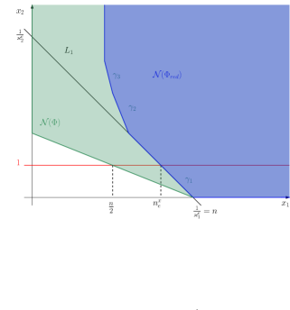
Figure 1. Effective Multiplicity

Next, somewhat in the spirit of Varchenko’s algorithm for constructing adapted coordinates for $\phi$ (see, e.g., [V76], [IM11a]), we shall allow for local coordinate changes (“non-linear shears”) of the form

(1.7) $$y_{1}:=x_{1}-{\alpha}(x_{2}),\quad y_{2}:=x_{2},$$

where ${\alpha}$ is smooth and vanishes at $x_{2}=0.$ Given such a coordinate system $y=(y_{1},y_{2}),$ we express $\phi$ in these coordinates by putting

$$\tilde{\phi}(y_{1},y_{2}):=\phi(y_{1}+{\alpha}(y_{2}),y_{2}).$$

Indeed, as will be discussed in more detail in Section 3, we can even allow for a more general class of local coordinate changes near the origin than in (1.7), of the form

(1.8) $$x_{1}:={\varphi}(y_{1},y_{2}),\quad x_{2}=y_{2},$$

where ${\varphi}$ is smooth, vanishes at the origin and ${\partial}_{1}{\varphi}(0,0)\neq 0.$ Such changes of coordinates will be called admissible. Here, we then put $\tilde{\phi}(y_{1},y_{2}):=\phi({\varphi}(y_{1},y_{2}),y_{2}).$

If we work in the category of analytic functions, we may and shall assume that the above changes of coordinates are analytic too, i.e., that ${\alpha}$ respectively ${\varphi}$ are analytic.

Note: The coordinates $(y_{1},y_{2})$ are also adapted to $\tilde{\phi}.$

Indeed, since $1/2>1/n,$ one easily checks that property (${\mathcal{A}}_{n-1}^{+}$) is preserved by these kind of coordinate changes (1.8).

We next decompose again $\tilde{\phi}(y_{1},y_{2})=\tilde{\phi}(0,y_{2})+\tilde{\phi}_{\rm red}(y_{1},y_{2})$ as we did for $\phi$ in (1.5), and compute for $\tilde{\phi}_{\rm red}$ as in (1.6) the corresponding number $n_{e}^{y}=(1-\tilde{\kappa}^{e}_{2})n,$ where $\tilde{\kappa}^{e}$ is the weight corresponding to the edge $\tilde{\gamma}_{1}$ with right endpoint $(n,0)$ of ${\mathcal{N}}(\tilde{\phi}_{\rm red}).$ Finally, we define

$$n_{e}=n_{e}(\phi):=\sup\limits_{y}n_{e}^{y},$$

where the supremum is taken over all analytic local coordinate systems $y=(y_{1},y_{2})$ of the form (1.8). Note also that $n_{e}\leq n.$

We shall show in Section 3 that this supremum is indeed a maximum, i.e., there exists a coordinate system $y=(y_{1},y_{2})$ such that $n_{e}^{y}=n_{e}.$ This coordinate system will even be of the form (1.7), so that it would indeed have sufficed to take the supremum over all coordinate systems (1.7) in the definition of $n_{e}.$ Any such coordinate system $y$ with $n^{y}=n_{e}$ will be called line-adapted to $\phi$ (not to be confused with the notion of “linearly adapted” coordinate systems introduced in [IM16]!), and the quantity $n_{e}$ will be called the effective multiplicity of $\phi.$ The latter notion is motivated by the following:

Given $n_{e},$ an important exponent for the study of the maximal operator ${\mathcal{M}}$ associated to $\phi$ will be given by

$$p_{e}:=\frac{2n_{e}}{n_{e}+1}.$$

For instance, every function which has a singularity of type $A_{n-1}$ can be written in suitable local coordinates in the normal form $\pm x_{2}^{2}\pm x_{1}^{n},$ which is of type ${\mathcal{A}}_{n-1}^{+}.$ For this normal form, we have ${\kappa}^{e}_{2}=0,$ and $n_{e}=n^{x}_{e}=(1-{\kappa}^{e}_{2})n=n.$

Thus, the exponent $p_{e}$ associated to $\phi$ before is formally the same as for the normal form $\pm x_{2}^{2}\pm x_{1}^{n_{e}}$ - this motivates our notion of effective multiplicity.

We remark that indeed also for ${\mathcal{A}}^{-}_{n-1}$ -singularities it is possible to define (in a less direct way) the notion of effective multiplicity (see Remark 10.2), so that this notion makes sense for any singularity of type ${\mathcal{A}}_{n-1}.$ However, we shall not really need to make use of this observation.

Remark 1.3.

If $\phi$ is of type ${\mathcal{A}}_{n-1}^{+},$ with $n\geq 4,$ then $p_{e}>h(\phi).$ Moreover, we always have $n<2n_{e},$ in particular $n_{e}>2,$ and $p_{e}\geq 3/2$ if and only if $n_{e}\geq 3.$

Indeed, we have $h=d={2n}/(n+2),$ and $p_{e}\geq{2n^{x}_{e}}/(n^{x}_{e}+1).$ And, a look at the Newton polyhedra of $\phi$ and $\phi_{\rm red}$ (cf. Figure 1) shows that the horizontal line $t_{2}=1$ intersects the principal face of ${\mathcal{N}}(\phi)$ at the $t_{1}$-coordinate $n/2<n_{e}^{x}\leq n_{e}.$ But, this implies that ${2n_{e}}/(n_{e}+1)>h.$ The remaining statements are immediate.

Let us present some examples of ${\mathcal{A}}_{n-1}^{+}$-type singularities. The first two examples show that the original coordinates $x$ may in general not be line-adapted, and that the inequality $n_{e}\leq n$ can indeed be strict:

Example 1.4.

Let $\phi(x_{1},x_{2}):=x_{2}^{2}+(x_{1}+x_{2}^{\ell})^{n},$ where $\ell\geq 2.$

Then $\phi_{\rm red}(x_{1},x_{2})=(x_{1}+x_{2}^{\ell})^{n}-x_{2}^{n\ell},$ so that ${\kappa}^{e}_{2}=1/n\ell,$ if $c\neq 0,$ hence

$$n_{e}^{x}=(1-\frac{1}{n\ell})n=n-\frac{1}{\ell}.$$

However, in the coordinates $y_{1}:=x_{1}+x_{2}^{\ell},y_{2}:=x_{2},$ we have $\tilde{\phi}(y_{1},y_{2})=y_{2}^{2}+y_{1}^{n},$ hence $n^{y}_{e}=n,$ so that $n_{e}=n.$ In particular, in contrast to the coordinates $x,$ the coordinates $y$ are line-adapted to $\phi$ (which follows easily from Proposition 3.1), and we have $p_{e}={2n}/(n+1).$

Example 1.5.

Let $\phi(x_{1},x_{2}):=(1+x_{1}^{\alpha}x_{2}^{\beta})x_{2}^{2}+x_{1}^{n},\qquad{\alpha},{\beta}\in{\mathbb{N}}.$

Here, if ${\alpha}\geq 1,$ then $\phi_{\rm red}(x_{1},x_{2})=x_{1}^{\alpha}x_{2}^{\beta}x_{2}^{2}+x_{1}^{n},$ and if ${\alpha}=0,$ then $\phi_{\rm red}(x_{1},x_{2})=x_{1}^{n}.$ Thus one computes that ${\kappa}^{e}_{2}=(n-{\alpha})/{n({\beta}+2)},$ if $1\leq{\alpha}<n,$ and ${\kappa}^{e}_{2}=n,$ if ${\alpha}\geq n.$ Hence, by (1.6), $n_{e}^{x}=(n({\beta}+1)+{\alpha})/({\beta}+2),$ if $1\leq{\alpha}<n,$ and $n_{e}^{x}=n,$ if ${\alpha}=0,$ or ${\alpha}\geq n.$ Moreover, it is easily seen that the coordinates $x$ are already line-adapted (which follows again from Proposition 3.1), and thus we have $n_{e}=n_{e}^{x}<n$ iff $1\leq{\alpha}<n.$ In particular, $p_{e}=2\big{(}n({\beta}+1)+{\alpha}\big{)}/\big{(}n({\beta}+1)+{\alpha}+{\beta}+2\big{)},$ if $1\leq{\alpha}<n,$ and $p_{e}=2n/(n+1),$ if ${\alpha}=0,$ or ${\alpha}\geq n.$

Example 1.6.

Let $\phi(x_{1},x_{2}):=\frac{1}{1-x_{1}}x_{2}^{2}+x_{1}^{n}.$

In contrast to Example 1.5, the graph of this function is convex for $|x_{1}|<1$ when $n$ is even. Since $1/(1-x_{1})=1+x_{1}+O(x_{1}^{2}),$ as in Example 1.5 we have $n_{e}^{x}=(n+1)/{2},$ and the coordinates $x$ are already line-adapted, so that $n_{e}=(n+1)/{2}$ and $p_{e}=2(n+1)/(n+3).$

Finally, for functions of type ${\mathcal{A}}_{n-1}^{+}$ let us put

$$\tilde{p}_{c}:=\max\{3/2,p_{e},h\}=\max\{3/2,p_{e}\},$$

where $h:=h(\phi)=h(x^{0},S).$ Note that in view of Remark 1.3 we have indeed that $\tilde{p}_{c}=\max\{3/2,p_{e}\}.$ The following result will be proven in Section 2:

Proposition 1.7.

Assume that $S$ is the graph of $1+\phi,$ and accordingly $x^{0}=(0,0,1),$ where $\phi$ is of type ${\mathcal{A}}_{n-1}^{+}$. Then, if $\rho(x^{0})\neq 0,$ the condition $p\geq\tilde{p}_{c}$ is necessary for ${\mathcal{M}}$ to be $L^{p}$-bounded.

Our main conjecture on the boundedness of the maximal operator ${\mathcal{M}}$ for singularities of type ${\mathcal{A}}_{n-1}^{+}$ states that the condition stated before is essentially also sufficient:

Conjecture 1.

Assume that $S$ is the graph of $1+\phi,$ and accordingly $x^{0}=(0,0,1),$ where $\phi$ is of type ${\mathcal{A}}_{n-1}^{+}.$ Then, if the density $\rho$ is supported in a sufficiently small neighborhood of $x^{0},$ the condition $p>\tilde{p}_{c}$ is sufficient for ${\mathcal{M}}={\mathcal{M}}_{\rho}$ to be $L^{p}$-bounded, so that indeed $p_{c}(x^{0})=\tilde{p}_{c}.$

We shall show that for a large class of functions $\phi$ of type ${\mathcal{A}}_{n-1}^{+}$ this conjecture indeed holds true. To describe this class, let us assume that $(y_{1},y_{2})$ is a line-adapted coordinate system in which the function $\phi(x_{1},x_{2})$ is represented by $\tilde{\phi}(y_{1},y_{2}).$

Assuming first that $\tilde{\kappa}^{e}_{2}>0,$ let us decompose the function $\tilde{\phi}_{\rm red}(y_{1},y_{2})=\tilde{\phi}(y_{1},y_{2})-\tilde{\phi}(0,y_{2})$ into

(1.9) $$\tilde{\phi}_{\rm red}(y_{1},y_{2})=p(y_{1},y_{2})+\tilde{\phi}_{\rm err}(y_{1},y_{2}),$$

with a $\tilde{\kappa}^{e}$-homogeneous polynomial $p$ of $\tilde{\kappa}^{e}$-degree 1 consisting of at least two monomial terms, with Taylor support on the first non-horizontal edge $\tilde{\gamma}_{1}$ of ${\mathcal{N}}(\tilde{\phi}_{\rm red}),$ which is compact and has right endpoint $(n,0)$ (and a remainder term $\tilde{\phi}_{\rm err}$ consisting of terms of higher $\tilde{\kappa}^{e}$-degree).

Assume next that $\tilde{\kappa}^{e}_{2}=0.$ Then $\tilde{\gamma}_{1}$ is vertical, and in this case $p(y_{1},y_{2})$ may no longer be a polynomial, but of the form $y_{1}^{n}G(y_{1},y_{2}),$ with $G$ analytic and $G(0,0)\neq 0.$

We shall be able to handle in this paper all functions of type ${\mathcal{A}}_{n-1}^{+}$, except for functions from a class that we shall denote by ${\mathcal{A}}_{n-1}^{e}.$ To facilitate notation, let us assume without loss of generality henceforth that $\beta(0)=1$ (see (1.3)).

The class of functions of type ${\mathcal{A}}_{n-1}^{+}\setminus{\mathcal{A}}_{n-1}^{e}$. By definition, these are those functions $\phi$ from ${\mathcal{A}}_{n-1}^{+}$ which satisfy the following assumptions:

Assume that $y=(y_{1},y_{2})$ is any line-adapted coordinate system. Then either $\tilde{\kappa}^{e}_{2}=0,$ or $\tilde{\kappa}^{e}_{2}>0,$ and the $\tilde{\kappa}^{e}$-homogeneous polynomial $p(y_{1},y_{2})$ satisfies the following two conditions:

• ${\partial}_{y_{1}}^{2}p(y_{1},y_{2})$ consists of at least two distinct monomial terms, one of them of course being $n(n-1)y_{1}^{n-2}.$

• If ${\partial}_{y_{1}}^{2}p(y_{1},y_{2})$ does not vanish of maximal possible order $n-2$ along a real, non-trivial root of ${\partial}_{y_{1}}^{2}p(y_{1},y_{2});$ more precisely, ${\partial}_{y_{1}}^{2}p(y_{1},y_{2})$ is not of the form

  (1.10) $${\partial}_{y_{1}}^{2}p(y_{1},y_{2})=n(n-1)(y_{1}-cy_{2}^{a})^{n-2},$$

  with $c\in{\mathbb{R}}\setminus\{0\}$ and integer exponent $a\in{\mathbb{N}}_{\geq 1}.$

On the exceptional class ${\mathcal{A}}_{n-1}^{e}$. We remark that if (1.10) is satisfied, i.e., if $\phi$ is of class ${\mathcal{A}}_{n-1}^{e},$ then ${\partial}_{y_{1}}p$ must be of the form ${\partial}_{y_{1}}p(y_{1},y_{2})=n(y_{1}-cy_{2}^{a})^{n-1}+c_{1}y_{2}^{a(n-1)},$ with $c_{1}\neq 0,$ for if $c_{1}=0,$ then the coordinates $y$ could not have been line-adapted by Corollary 3.5. Consequently, we would have

$$p(y_{1},y_{2})=(y_{1}-cy_{2}^{a})^{n}+c_{1}y_{1}y_{2}^{a(n-1)}+c_{0}y_{2}^{an},\qquad\text{with}\ c_{1}\neq 0.$$

Note that we could here perform a change of coordinates $u_{1}:=y_{1}-cy_{2}^{a},u_{2}=y_{2},$ so that in the new coordinates $u=(u_{1},u_{2}),$ we would have

$$p(y_{1},y_{2})=u_{1}^{n}+c_{1}u_{1}u_{2}^{a(n-1)}+(c_{0}+cc_{1})u_{2}^{an},$$

where $a(n-1)\geq 3,$ if $n\geq 3,$ so that we may write $a(n-1)=\beta+2,$ with $\beta\in{\mathbb{N}}.$ Since the last term depends on $u_{2}$ only, if then we look at the function $\tilde{\tilde{\phi}}(u_{1},u_{2})$ which represents $\phi$ in these coordinates, we see that $\tilde{\tilde{\phi}}_{\rm red}(u_{1},u_{2})$ is of the form

$$\tilde{\tilde{\phi}}_{\rm red}(u_{1},u_{2})=u_{1}^{n}+c_{1}u_{1}u_{2}^{\beta+2}+\tilde{\tilde{\phi}}_{\rm err}(u_{1},u_{2}),$$

and by the discussion in Section 3 it is easy to see that the coordinates $u$ are line-adapted too. Up to the error term, we see that this is now of the form described in Example 1.5, with ${\alpha}=1.$

On the other hand, if we assume that $(A1)$ is not satisfied, then we see that $p(y_{1},y_{2})$ must be of the form

$$p(y_{1},y_{2})=y_{1}^{n}+c_{1}y_{1}y_{2}^{k},$$

with $c_{1}\neq 0,$ and since $\tilde{\kappa}^{e}_{2}<1/2,$ it is easily seen that $k\geq 2,$ so that again

(1.11) $$p(y_{1},y_{2})=y_{1}^{n}+c_{1}y_{1}y_{2}^{\beta+2},\qquad\text{with}\ \beta\in{\mathbb{N}}.$$

Thus, we see that $\phi$ is of exceptional type ${\mathcal{A}}_{n-1}^{e}$ if and only if there is a line-adapted coordinate system in which $p(y)$ is of the form (1.11).

If we look at the examples, we thus see that the functions $\phi$ in Example 1.5 are of type ${\mathcal{A}}_{n-1}^{e}$ if and only if ${\alpha}=1.$ Another example of type ${\mathcal{A}}_{n-1}^{e}$ is Example 1.6, which is a variant of the case ${\alpha}=1,\beta=0$ in Example 1.5 in which $\phi$ is even convex whenever $n\geq 2$ is an even number.

Example 1.8.

Let $\phi(x_{1},x_{2}):=x_{2}^{2}+(x_{1}+x_{2}^{\ell})x_{2}^{k}+(x_{1}+x_{2}^{\ell})^{n},$ where $k\geq 2,\ell\geq 1$ and $\ell(n-1)<k.$

Here one checks that ${\kappa}_{1}^{e}=1/n,{\kappa}_{2}^{e}=1/n\ell.$ If we pass to the admissible coordinates $(y_{1},y_{2})$ with $y_{1}:=x_{1}+x_{2}^{\ell},y_{2}:=x_{2},$ then $\phi$ is represented by $\tilde{\phi}(y_{1},y_{2})=y_{2}^{2}+y_{1}y_{2}^{k}+y_{1}^{n},$ with $\tilde{\kappa}_{1}^{e}=1/n,\tilde{\kappa}^{e}_{2}=(n-1)/nk.$ And, one easily verifies by means of Proposition 3.1 that the coordinates $(y_{1},y_{2})$ are line-adapted to $\phi,$ whereas the coordinates $(x_{1},x_{2})$ are not, since $1/{\kappa}^{e}_{2}<1/\tilde{\kappa}^{e}_{2}.$ Moreover, $\tilde{\phi}_{\rm red}(y_{1},y_{2})=y_{1}y_{2}^{k}+y_{1}^{n},$ which shows that $\phi$ is of type ${\mathcal{A}}_{n-1}^{e}.$

Our main result on functions of type ${\mathcal{A}}_{n-1}^{+}$ in this paper is

Theorem 1.9.

Assume that $S$ is the graph of $1+\phi,$ and accordingly $x^{0}=(0,0,1),$ where $\phi$ is analytic and of type ${\mathcal{A}}_{n-1}^{+}\setminus{\mathcal{A}}_{n-1}^{e}$. Then, if the density $\rho$ is supported in a sufficiently small neighborhood of $x^{0},$ the condition $p>\max\{3/2,p_{e}\}$ is sufficient for ${\mathcal{M}}$ to be $L^{p}$-bounded. Moreover, if $\rho(x^{0})\neq 0,$ it is also necessary. I.e., in this case we have $p_{c}(x^{0})=\max\{3/2,p_{e}\}.$

We shall turn to the remaining exceptional class of functions of type ${\mathcal{A}}_{n-1}^{e}$ in the third paper of this series. However, in the last Section 14, we shall at least show that the condition $p>\max\{3/2,2n/(n+1)\}$ is sufficient for ${\mathcal{M}}$ to be $L^{p}$-bounded. In combination with all other results, this will lead to a proof of a conjecture by Iosevich-Sawyer-Seeger for arbitrary analytic 2-surfaces (compare Subsection 2.2).

1.3. A more general conjecture in arbitrary dimension

Let us come back to more general hypersurfaces $S\subset{\mathbb{R}}^{d}$ and their associated maximal operators ${\mathcal{M}}$ as discussed at the beginning of this section. Assuming that $S$ satisfies the transversality Assumption 1.1 near a given point $x^{0}\in S$ and is contained in a sufficiently small neighborhood of $x^{0}$ (as in the 3-dimensional case) we may assume that, after applying a suitable linear change of coordinates in ${\mathbb{R}}^{d},$ we have $x^{0}=(0,1)$ with respect to the splitting ${\mathbb{R}}^{d}={\mathbb{R}}^{d-1}\times{\mathbb{R}},$ and that $S$ is the graph

$$S=\{(x^{\prime},1+\phi(x^{\prime})):x^{\prime}\in{\Omega}\}$$

of a smooth function $1+\phi$ defined on an small open neighborhood ${\Omega}$ of $0\in{\mathbb{R}}^{d-1}$ satisfying

$$\phi(0)=0,\,\nabla\phi(0)=0.$$

By localizing to a sufficiently small neighborhood of $x^{0},$ we may also assume that

(1.12) $${\Omega}={\Omega}_{\varepsilon}=\{z^{\prime}\in{\mathbb{R}}^{d-1}:|z^{\prime}|<{\varepsilon}\}\quad\text{and}\quad|\nabla\phi(z^{\prime})|\leq\frac{1}{10}\quad\text{for all }z^{\prime}\in{\Omega},$$

where $0<{\varepsilon}<1$ can be assumed to be small.

Let us also assume here that $\rho\geq c>0$ on $S.$ Then, without loss of generality, we may even assume that

(1.13) $$A_{t}f(y)=\int_{\Omega}f(y^{\prime}-tx^{\prime},y_{d}-t(1+\phi(x^{\prime})))\,dx^{\prime}.$$

The following proposition, which yields necessary conditions of geometric measure theoretic type for the $L^{p}$- boundedness of the maximal operator ${\mathcal{M}}_{S},$ will be proved in Section 2 under these assumptions.

Proposition 1.10.

Let $T\subset{\mathbb{R}}^{d}$ be a symmetric convex body of positive volume $|T|>0$. Assume further that (1.12) is satisfied, and let $z_{d}:{\Omega}_{\varepsilon}\to{\mathbb{R}}$ be any $C^{1}$- function so that

(1.14) $$z_{d}(0)=1,\quad\nabla z_{d}(0)=0,\quad\text{and}\quad|\nabla z_{d}(z^{\prime})|\leq\frac{1}{6}\quad\text{for all }\ z^{\prime}\in{\Omega}_{\varepsilon}.$$

Put $T(z^{\prime}):=(z^{\prime},z_{d}(z^{\prime}))+T$ for $z^{\prime}\in{\Omega}_{\varepsilon},$ and

$$|T(z^{\prime})\cap S|:=\int_{{\Omega}_{\varepsilon}}\chi_{T(z^{\prime})}(x^{\prime},1+\phi(x^{\prime}))\,dx^{\prime}.$$

Then, for $1\leq p<\infty,$ we have

$$\int_{{\Omega}_{\varepsilon}}\frac{|T(z^{\prime})\cap S|^{p}}{|T|}\,dz^{\prime}\leq 4(C_{d}{\varepsilon}^{d-1})^{-p}\|{\mathcal{M}}\|_{L^{p}\to L^{p}}^{p}.$$

Remarks 1.11.

(i) The same result would hold more generally for any star-shaped body $T,$ but that fact does not seem to be relevant for our applications.

(ii) In view of John’s theorem, we may basically replace the class of all convex bodies $T$ in this result by the class of all ellipsoids centered at the origin.

(iii) Our proof will show that we even have the estimate

$$\int_{{\Omega}_{\varepsilon}}\frac{|T(z^{\prime})\cap S|^{p}}{|T|}\,dz^{\prime}\leq 4(C_{d}{\varepsilon}^{d-1})^{-p}\|{\mathcal{M}}_{\rm loc}\|_{L^{p}\to L^{p}}^{p},$$

where

$${\mathcal{M}}_{\rm loc}f(x):=\sup_{1/2\leq t\leq 1}|A_{t}f(x)|.$$

Under the assumptions (1.12) on $\phi,$ let us put

$$p_{\rm geom}(x^{0}):=\inf p,$$

where the infimum is taken over all $p\geq 1$ for which there is some ${\varepsilon}>0,$ and a constant $C_{p,{\varepsilon}}\in{\mathbb{R}}$ such that

$$\int_{{\Omega}_{\varepsilon}}\frac{|T(z^{\prime})\cap S|^{p}}{|T|}\,dz^{\prime}\leq C_{p,{\varepsilon}}$$

holds true for all ellipsoids $T$ centered at the origin and all $C^{1}$-functions $z_{d}:{\Omega}_{\varepsilon}\to{\mathbb{R}}$ satisfying the assumptions (1.14).

As a corollary to Proposition 1.10, we obtain

Corollary 1.12.

If $p<p_{\rm geom}(x^{0}),$ then the maximal operators ${\mathcal{M}}$ is unbounded on $L^{p}({\mathbb{R}}^{d}),$ so that in particular $p_{\rm geom}(x^{0})\leq p_{c}(x^{0}).$

Conjecture 2.

If $p>p_{\rm geom}(x^{0}),$ then the maximal operator ${\mathcal{M}}={\mathcal{M}}_{\rho}$ is bounded on $L^{p}({\mathbb{R}}^{d}),$ provided $\rho$ is supported in a sufficiently small neighborhood of $x^{0},$ so that indeed $p_{c}(x^{0})=p_{\rm geom}(x^{0}).$

Our discussion in Section 2 will reveal that this conjecture holds indeed true in dimension $d=3,$ with the possible exception of hypersurfaces of type ${\mathcal{A}}^{e},$ for which, however, it is equivalent to Conjecture 1.

1.4. A guide through the organization of the paper and the proofs of our main results

Section 2 will be devoted to the proof of Proposition 1.10, from which we shall also deduce the necessity of the conditions in our main Theorems 1.2 and 1.9. Moreover, we shall compare our results with results and a conjecture by Iosevich, Sawyer and Seeger from their article [ISaSe99].

In preparation of the proof of Theorem 1.9, in Sections 3 and 4 we shall study functions $\phi=\phi(x_{1},x_{2})$ of type ${\mathcal{A}}^{+}_{n-1}$ and their Legendre transforms $\breve{\phi}=\breve{\phi}(x_{1},s_{2})$ with respect to the second variable $x_{2}.$ The latter will be crucial in order to obtain very precise information on the partial Fourier transform of the measure $\mu$ with respect to $x_{2}.$ In particular, we shall show in Section 3 how to construct line-adapted coordinates for $\phi,$ and give a necessary and sufficient condition for a given coordinate system to be line-adapted. And, in Section 4, we shall show that the classes ${\mathcal{A}}^{+}_{n-1}$ and ${\mathcal{A}}^{e}_{n-1}$ are invariant under this Legendre transform, and that the principal parts $\phi_{\rm red}$ of $\phi$ and $\breve{\phi}_{\rm red}$ of $\breve{\phi}$ are “essentially” the same, a fact which will be crucial in order to be able to transfer the conditions $(A1),(A2)$ on $\phi_{\rm red}$ into the same conditions on $\breve{\phi}_{\rm red}.$

Next, in Section 5, we shall provide some auxiliary results which will be used frequently later on. First, we recall a well-know version of a van der Corput type estimate for one-dimensional oscillatory integrals. Then, in Lemma 5.2, we prove an identity for two-dimensional oscillatory integrals which has the flavour of a stationary phase identity and which will become crucial later on whenever we shall have to deal with the most challenging oscillatory integrals arising in our later studies. Next, we shall recall a lemma from our preceding paper [BDIM19] which will be applied whenever we shall prove $L^{p}$ - estimates for $p$ close to $1$ for maximal operators associated to “microlocalized” pieces of our measure $\mu.$ Finally, we shall perform some preliminary reductions which will allow to spectrally localize the measure $\mu$ to frequencies $\xi=(\xi_{1},\xi_{2},\xi_{3})$ where

$$|\xi_{3}|\sim{\lambda}\gg 1\text{ and }|s_{1}|,|s_{2}|\ll 1,\text{ with }s_{1}:=\frac{\xi_{1}}{\xi_{3}},s_{2}:=\frac{\xi_{2}}{\xi_{3}},s_{3}:=\frac{\xi_{3}}{{\lambda}}.$$

Here,${\lambda}$ is a dyadic number, and the resulting measure will be denoted by $\mu^{\lambda}.$

The Sections 6 to 9 will be devoted to the proof of the sufficiency of the conditions in Theorem 1.2. We begin by applying the method of stationary phase in the coordinate $x_{2};$ in particular, we determine the Legendre transform $\breve{\phi}(x_{1},s_{2})$ (cf. (6.2)) and show that the Fourier transform of $\mu^{\lambda}$ can be written as

$$\widehat{\mu^{\lambda}}(\xi)={\lambda}^{-\frac{1}{2}}e^{-i{\lambda}s_{3}\big{(}s_{2}^{2}B(s_{2})+1\big{)}}J({\lambda},s)\,\chi_{0}(s_{3}s^{\prime})\chi_{1}(s_{3}),$$

where $J({\lambda},s)$ denotes the one-dimensional oscillatory integral

$$J({\lambda},s):=\int e^{-i{\lambda}s_{3}\Phi_{0}(x_{1},s^{\prime})}\eta(x_{1},s_{2})\,dx_{1},$$

with phase $\Phi_{0}(x_{1},s^{\prime}):=\breve{\phi}_{1}(x_{1},s_{2})+s_{1}x_{1},$ where $s^{\prime}:=(s_{1},s_{2}).$ Quite important for us will also be the two-dimensional oscillatory integral

$$F({\lambda},s_{2},s_{3},y_{1}):=\iint e^{-i{\lambda}s_{3}(\Phi_{0}(x_{1},s^{\prime})-s_{1}y_{1})}\eta(x_{1},s_{2})\chi_{0}(s_{3}s^{\prime})\chi_{0}(s_{1})\,dx_{1}ds_{1},$$

which will allow us to write

$$\mu^{\lambda}(y+{\Gamma})={\lambda}^{\frac{5}{2}}\int\Big{(}\int F({\lambda},s_{2},s_{3},y_{1})e^{-i{\lambda}s_{3}(s_{2}^{2}B(s_{2})-s_{2}y_{2}-y_{3})}\chi_{0}(s_{2})ds_{2}\Big{)}\chi_{1}(s_{3})ds_{3},$$

where we have put $\Gamma:=(0,0,1).$

Our estimates for the maximal operator ${\mathcal{M}}^{\lambda}$ associated to the measure $\mu^{\lambda}$ will be based on an interpolation between $L^{2}$ - estimates and $L^{1+{\varepsilon}}$ - estimates for ${\varepsilon}>0$ sufficiently small. In view of Plancherel’s theorem, for these $L^{2}$- estimates, we shall need to estimate the oscillatory integrals $J({\lambda},s),$ whereas for our $L^{1+{\varepsilon}}$-estimates, pointwise bounds on $\mu^{\lambda}(y+{\Gamma})$ will be required in order to be able to apply Lemma 5.4.

As for the oscillatory integral $J({\lambda},s),$ which strongly depends on the parameter $s_{2},$ the strategy will be to fix a certain dyadic level of $s_{2},$ say where $s_{2}\sim 2^{-k}\ll 1,$ and then try to decompose the support of $\eta$ in $x_{1}$ into intervals over which the second derivative

$$\Phi(x_{1},s_{2}):={\partial}_{x_{1}}^{2}\Phi_{0}(x_{1},s^{\prime})={\partial}_{x_{1}}^{2}\breve{\phi}_{1}(x_{1},s_{2})$$

will essentially be of a certain level size for these values of $s_{2},$ so that for these parts of the oscillatory integral we can apply van der Corput’s estimate of order $2.$ Clearly, in order to perform this, we shall need to understand the null set $\Phi(x_{1},s_{2})=0.$ It is well-known that this set is the union of finitely many curves, either of the form $x_{1}=0,$ or $x_{1}=r(s_{2}),$ with non-trivial “real roots” $r(s_{2})$ which can be expanded as Puiseux series in $s_{2}$ – these facts will be re-called in Subsection 6.2, as well as their connections with the two-dimensional Newton-polyhedron ${\mathcal{N}}(\Phi)$ associated to $\Phi.$ We are here following ideas from [PS97]. These roots come in clusters, the first type of cluster being determined by the leading exponent of the roots (we also have to consider complex roots!). These in return are in one to one correspondence with the compact edges of ${\mathcal{N}}(\Phi):$ if $a=a_{l}$ is the leading exponent of all roots in a given cluster, then there is a unique compact edge ${\gamma}={\gamma}_{l}$ such that $a$ is just the modulus of the slope of this edge.

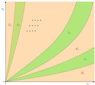
Figure 3. Domain Decomposition

Moreover, each compact edge ${\gamma}_{l}$ comes with a certain (typically) anisotropic scaling structure, which allows to decompose our $(x_{1},s_{2})$ - domain into certain domains $D_{l}$ which are invariant under the scalings associated to ${\gamma}_{l},$ and transition domains $E_{l}$ in between these homogeneous domain (see Figure 3). This decomposition will be explained in Section 7. Now, on each transition domain, it turns out that we do have a good resolution of singularities of $\Phi;$ indeed, by (7.5),

$$\Phi(x_{1},s_{2})=V(x_{1},s_{2})\,s_{2}^{A_{l}}x_{1}^{B_{l}},\qquad(x_{1},s_{2})\in E_{l},$$

where $|V(x_{1},s_{2})|\sim 1,$ and where $(B_{l},A_{l})$ is a vertex of ${\mathcal{N}}(\Phi)$ associated to $E_{l}.$ Thus, if we assume that $x_{1}\sim 2^{j},$ then we see that $|\Phi(x_{1},s_{2})|\sim 2^{-kA_{l}-jB_{l}},$ so that we can apply van der Corput’s estimate to the corresponding part $J_{j,k}({\lambda},s)$ of $J({\lambda},s)$ and get an appropriate $L^{2}$ - estimate for the associated maximal operator ${\mathcal{M}}^{\lambda}_{j,k}.$

However, a considerably bigger challenge comes with the $L^{1+{\varepsilon}}$ - estimates of ${\mathcal{M}}^{\lambda}_{j,k}.$ Here, we need to understand the original phase $\Phi_{0}$ and the associated functions $F_{j,k}$ and $\mu^{\lambda}_{j,k}.$ We show in (7.6) that, for suitable functions $g$ and $h,$

$$\Phi_{0}(x_{1},s^{\prime})=\breve{\phi}_{1}(x_{1},s_{2})+s_{1}x_{1}=U(x_{1},s_{2})s_{2}^{A_{l}}x_{1}^{B_{l}+2}+x_{1}(s_{1}+g(s_{2}))+h(s_{2}),$$

where $|U(z_{1},s_{2})|\sim 1,$ and one problem will be to gain a suitable control on these functions $g$ and $h$ (which is not very difficult in this first step of our resolution algorithm, but becomes more involved later on) in order to later also be able to control the integration in $s_{2}$ in our integral formula for $\mu^{\lambda}(y+{\Gamma}).$

Once the $L^{1+{\varepsilon}}$ - estimates are established, we can interpolate in order to obtain $L^{p}$-estimates for the maximal operators ${\mathcal{M}}^{\lambda}_{j,k}.$ In order to show that these estimates can indeed be summed over all dyadic ${\lambda}\gg 1$ and all indices $j,k$ associated to the domain $E_{l},$ we also need the important “Geometric Lemma” 7.3 and its corollary, Lemma 7.4, which will allow us to relate information from the Newton polyhedron to the exponents which appear in our $L^{p}$-estimates.

We are then left with the contributions by the homogeneous domains $D_{l},$ which will contain all real “root curves” of the associated cluster. Given any leading term $cs_{2}^{a}$ of some real root in the cluster, we can then essentially localize to a narrow, homogeneous neighborhood of the curve $x_{1}=cs_{2}^{a},$ which will contain all “root curves” with this leading term.

In order to study the contribution by this narrow domain, we perform a change of coordinates, by putting $x_{1}-cs_{2}^{a}=:\tilde{z},$ and express everything in these new coordinates $(\tilde{z},s_{2})$ in place of $(x_{1},s_{2}).$ In particular, we can then express the function $\Phi(x_{1},s_{2})$ as a function $\tilde{\Phi}(\tilde{z},s_{2}).$ All this will be done in Section 7.

In a second step of our resolution of singularities algorithm, we shall then consider the Newton polyhedron ${\mathcal{N}}(\tilde{\Phi}),$ and try to iterate the procedure from the first step, with $\Phi$ replaced by $\tilde{\Phi}.$ This will be performed in Section 8. The $L^{1+{\varepsilon}}$ - estimates for the corresponding transition domains $\tilde{E}_{l}$ will become even more involved in this Step 2. There are many subtleties arising in this process, let us just highlight one: Lemma 7.4 requires that the first compact edge of the Newton polyhedron has a left endpoint $(B_{1},A_{1})$ with $A_{1}\geq 1.$ This is immediate in Step 1, but no longer in Step 2, where this condition may fail. But, it turns out that the cases where this happens to fail can still be handled, since we do have a good resolution of singularities in these cases (see Subsection 8.1).

Proceeding in this way with our algorithm, in order to analyze the contributions by the new homogeneous domains $\tilde{D}_{l},$ we have again to perform changes of coordinates by subtracting second order terms of the Puiseux series expansions of roots from $\tilde{z},$ in order to arrive at Step 3, and so forth. All this will be explained in Section 9. Iterating this procedure, we shall, step by step, narrow down our considerations to smaller and smaller homogeneous domains containing only root curves from sub-clusters of higher and higher order, which, after a finite number of steps, will only contain one, real root $r(s_{2}),$ but possibly with multiplicity. However, in this case one can obtain a good resolution of singularity near this root, and can then essentially apply the same techniques that we had used for transition domains also to such kind of homogeneous domains.

The Sections 10 to 13 will be covering the proof of the sufficiency of the conditions in Theorem 1.9. By and large, we shall be able to follow the proof of Theorem 1.2 and shall therefore only highlight those parts of the proof which will require different or modified arguments. Major differences are caused by the change of coordinates (1.7) which leads to line-adapted coordinates. Moreover, a crucial new tool will be the “Multiplicity Lemma“ 11.1, which, under our assumptions $(A1),(A2),$ implies that in Step 2 of our resolution algorithm, the case where $A_{1}<1$ can only arise when all non-trivial real roots have multiplicity $1,$ so that we can then argue in a similar way as for Theorem 1.2. Another difference is the way how we control the functions $g$ and $h$ above; this, however, turns out to be even easier here than in the case of singularities of type ${\mathcal{A}}^{-}_{n-1},$ due to the fact that here $\tilde{\kappa}^{e}_{2}<1/2.$

Finally, in Section 14, we shall indicate how the proof of Theorem 1.9 can be modified to give a proof of the Iosevich-Sawyer-Seeger conjecture for surfaces of class ${\mathcal{A}}^{e}_{n-1}.$

Conventions: Throughout this article, we shall use the “variable constant” notation, i.e., many constants appearing in the course of our arguments, often denoted by $C,$ will typically have different values at different lines. Moreover, we shall use symbols such as $\sim,\lesssim$ or $\ll$ in order to avoid writing down constants, as explained in [IM16, Chapter 1]. By $\chi_{0}$ and $\chi_{1}$ we shall denote smooth cut-off functions on ${\mathbb{R}}$ with typically small compact supports, where $\chi_{1}$ vanishes near the origin and is identically one near $1,$ whereas $\chi_{0}$ is identically $1$ on a small neighborhood of the origin. These cut-off functions may also vary from line to line, and may in some instances, where several of such functions of different variables appear within the same formula, even designate different functions.

Also, if we speak of the slope of a line such as a supporting line to a Newton polyhedron, then we shall actually mean the modulus of the slope.

Acknowledgement: The authors wish to thank Spyros Dendrinos for helpful annotations on the paper and in particular for suggesting Example 1.6.

2. Necessary conditions

Let us first prove Proposition 1.10.

Proof of Proposition 1.10. Recall that ${\Omega}={\Omega}_{\varepsilon}=\{z^{\prime}\in{\mathbb{R}}^{d-1}:|z^{\prime}|<{\varepsilon}\},$ where $0<{\varepsilon}<1,$ and let

$$B:=\{t(z^{\prime},z_{d}(z^{\prime})):z^{\prime}\in\Omega,1/2\leq t\leq 1\}.$$

If $y\in B$, then $y=t(z^{\prime},z_{d}(z^{\prime}))=tz$, for suitable $t=t(y),z^{\prime}=z^{\prime}(y)$ and $1/2\leq t\leq 1$. Then, by (1.13), for such $y,t,z$,

$$A_{t}\chi_{T}(y) = \int_{\Omega}\chi_{T}(y^{\prime}-tx^{\prime},y_{d}-t(1+\phi(x^{\prime})))\,dx^{\prime}$$

$$= \int_{\Omega}\chi_{\frac{1}{t}(y+T)}(x^{\prime},1+\phi(x^{\prime}))dx^{\prime}$$

$$\geq C_{d}{\varepsilon}^{d-1}|T(z^{\prime})\cap S|,$$

since $T$ is symmetric and convex, which implies that $\frac{1}{t}(y+T)\supset T(z^{\prime})$. Thus,

$$|T(z^{\prime})\cap S|\leq\frac{1}{C_{d}{\varepsilon}^{d-1}}{\mathcal{M}}\chi_{T}(tz)$$

for $1/2\leq t\leq 1$. But, $F:(t,z^{\prime})\mapsto(tz^{\prime},tz_{d}(z^{\prime}))=tz$ is a $C^{1}$- change of coordinates, with Jacobian $J_{F}$ satisfying

$$|J_{F}(t,z^{\prime})|=t^{d-1}|z_{d}(z^{\prime})-z^{\prime}\cdot\nabla z_{d}(z^{\prime})|,$$

so that, by (1.14), $1/2^{d}\leq|J_{F}(t,z^{\prime})|\leq 2.$ Hence

$$\int_{\Omega}|T(z^{\prime})\cap S|^{p}dz^{\prime} \leq 2(C_{d}{\varepsilon}^{d-1})^{-p}\int_{\Omega}\int_{1/2}^{1}{\mathcal{M}}\chi_{T}(tz^{\prime},tz_{d}(z^{\prime})))^{p}dtdz^{\prime}$$

$$\leq 4(C_{d}{\varepsilon}^{d-1})^{-p}\int_{B}{\mathcal{M}}\chi_{T}(y)^{p}dy$$

$$\leq 4(C_{d}{\varepsilon}^{d-1})^{-p}\|{\mathcal{M}}\|^{p}_{p\to p}|T|.$$

Q.E.D.

In applications one would choose the function $z_{d}(z^{\prime})$ so that $|T(z^{\prime})\cap S|$ becomes essentially as large as possible.

2.1. The three dimensional case

Let us now turn our attention to the $d=3$ case. We will be looking at $T$ of the form $T=[-{\delta}_{1},{\delta}_{1}]\times[-{\delta}_{2},{\delta}_{2}]\times[-{\delta}_{3},{\delta}_{3}]$ with ${\delta}_{i}\leq 1.$ Let

$$I:=\{i\in\{1,2\}:{\delta}_{i}\sim 1\}.$$

We will be taking ${\delta}_{i}\ll 1$ for $i\not\in I$. Also let $k:=|I|$ and, given $z^{\prime}=(z_{1},z_{2})\in{\Omega},$ let us consider $(z_{1}^{0},z_{2}^{0}),$ where $z_{i}^{0}:=0,$ if $i\in I,$ and $z_{i}^{0}:=z_{i},$ if $i\not\in I$. It is then plausible that a good choice for the function $z_{3}(z_{1},z_{2})$ might be

(2.1) $$z_{3}(z_{1},z_{2}):=1+\phi(z_{1}^{0},z_{2}^{0}).$$

We deduce necessary conditions for the $L^{p}$-boundedness of ${\mathcal{M}}$ based on the following three examples, where the cases $k=0$ and $k=2$ can indeed by treated by this kind of choice of $z_{3}(z_{1},z_{2}).$ In the case $k=1,$ we will first have to apply suitable changes of coordinates of the form (1.7) before making this kind of choice.

Example 2.1.

The case $k=0$.

Here $I=\emptyset$, i.e., ${\delta}_{i}\ll 1,i=1,2,3$, and we choose $z_{3}(z_{1},z_{2}):=1+\phi(z_{1},z_{2})$. Then if we choose ${\delta}_{1}={\delta}_{2}={\delta}_{3}={\delta}\ll 1$, meaning that $T$ is a $\delta$-cube, we have $|T(z_{1},z_{2})\cap S|\sim{\delta}^{2}$ for all $(z_{1},z_{2})\in{\Omega}$, which implies that for all ${\delta}\ll 1,$

$$\|{\mathcal{M}}\|^{p}_{p\to p}\gtrsim\int_{\Omega}{\delta}^{2p-3}dz_{1}dz_{2}\sim{\delta}^{2p-3},$$

giving the necessary condition $p\geq 3/2$ ${\mathcal{M}}$ to be bounded on $L^{p}.$

Example 2.2.

The case $k=2$.

Here we choose $I=\{1,2\}$, hence only ${\delta}_{3}={\delta}\ll 1,$ and thus $T$ is essentially a ${\delta}$-slab. We choose $(z_{1}^{0},z_{2}^{0})=(0,0)$, so $z_{3}(z_{1},z_{2})=1+\phi(0,0)=1$. Then, the condition $|1+\phi(z_{1},z_{2})-z_{3}|=|\phi(z_{1},z_{2})|<{\delta}$ implies that $|T(z_{1},z_{2})\cap S|\sim{\delta}^{1/h}$ for all $(z_{1},z_{2})\in{\Omega}$ (i.e., $|(z_{1},z_{2})|<{\varepsilon}$), provided ${\varepsilon}>0$ is chosen sufficiently small. Here, $h=h(x^{0})$ denotes the height of $\phi$. This in turn implies that

$$\|{\mathcal{M}}\|^{p}_{p\to p}\gtrsim_{\varepsilon}\int_{\Omega}{\delta}^{p/h-1}dz_{1}dz_{2}\sim{\delta}^{p/h-1},$$

giving the necessary condition $p\geq h$ for ${\mathcal{M}}$ to be bounded on $L^{p}.$

Note that the same computations show that necessarily

(2.2) $$p_{\rm geom}\geq\max\{3/2,h\}.$$

Since we have seen in the Introduction that (1.4) holds true for all classes of 2-hypersurfaces, with the exception of hypersurfaces of type ${\mathcal{A}}_{n-1}^{+},$ and since by Corollary 1.12 we have $p_{\rm geom}\leq p_{c},$ (2.2) shows that indeed $p_{\rm geom}=p_{c}$ for these classes of surfaces.

Example 2.3.

The case $k=1$.

We can here focus on the remaining class of functions of type ${\mathcal{A}}_{n-1}^{+}.$ Following the discussion in Section 1 just before Examples 1.4 and 1.5, we may perform any local coordinate change as in (1.7) and denote by $y=(y_{1},y_{2})$ the new coordinate system.

Recall the decomposition $\phi(x_{1},x_{2})=\tilde{\phi}(y_{1},y_{2})=\tilde{\phi}(0,y_{2})+\tilde{\phi}_{\rm red}(y_{1},y_{2})$. Note that $\tilde{\phi}(0,y_{2})=y_{2}^{2}\rho(y_{2})$ for some analytic function $\rho$ at the origin. Denote by $\tilde{\gamma}_{1}$ the first edge of the Newton polyhedron ${\mathcal{N}}(\tilde{\phi}_{\rm red})$ of $\tilde{\phi}_{\rm red}$ with left endpoint $(n,0)$ (which must intersect the line $t_{2}=1$), and by $\tilde{L}_{1}:=\{\tilde{\kappa}^{e}_{1}t_{1}+\tilde{\kappa}^{e}_{2}t_{2}=1\}$ the line supporting $\tilde{\gamma}_{1}.$ Then $\tilde{\kappa}^{e}_{1}n_{y}^{e}+\tilde{\kappa}^{e}_{2}=1,$ hence (cf. (1.6))

$$n_{e}^{y}=(1-\tilde{\kappa}^{e}_{2})/\tilde{\kappa}^{e}_{1}.$$

Assume first that $\tilde{\kappa}^{e}_{2}>0,$ so that $\tilde{\gamma}_{1}$ is a compact edge.

We choose $I=\{1\}$, so that

$$T=[-1,1]\times[-{\delta}_{2},{\delta}_{2}]\times[-{\delta},{\delta}],$$

and then choose $z_{3}$ according to (2.1), but with respect to the coordinates $(y_{1},y_{2})$. Noting that $y_{2}=x_{2},$ this means that we put

$$z_{3}(z_{1},z_{2}):=1+\tilde{\phi}(0,z_{2})=1+z_{2}^{2}\rho(z_{2}).$$

Assume that the point $(x_{1},x_{2},1+\phi(x_{1},x_{2}))$ on $S$ lies in $T(z_{1},z_{2}).$ Then

$$|x_{1}-z_{1}|\leq 1,\ |x_{2}-z_{2}|\leq{\delta}_{2},\ |1+\phi(x_{1},x_{2})-z_{3}(z_{1},z_{2})|\leq{\delta}.$$

But, we have

(2.3) $$|1+\phi(x_{1},x_{2})-z_{3}(z_{1},z_{2})| = |1+\tilde{\phi}(y_{1},y_{2})-z_{3}(z_{1},z_{2})|$$

$$\leq |y_{2}^{2}\rho(y_{2})-z_{2}^{2}\rho(z_{2})|+|\tilde{\phi}_{\rm red}(y_{1},y_{2})|.$$

Note next that since $\tilde{\phi}_{\rm red}$ agrees with a $\tilde{\kappa}^{e}$-homogeneous polynomial of degree $1,$ up to some error term of higher $\tilde{\kappa}^{e}$-degree, we see that

$$|\tilde{\phi}_{\rm red}(y_{1},y_{2})|\lesssim|y_{1}|^{1/\tilde{\kappa}^{e}_{1}}+|y_{2}|^{1/\tilde{\kappa}^{e}_{2}},$$

provided ${\varepsilon}>0$ is sufficiently small in our definition of ${\Omega}.$ We also recall that $\tilde{\kappa}^{e}_{1}=1/n.$

Thus, to make sure that $|\tilde{\phi}_{\rm red}(y_{1},y_{2})|\leq{\delta}/2,$ it suffices to assume that

$$|x_{1}-\alpha(x_{2})|=|y_{1}|\leq c{\delta}^{\tilde{\kappa}^{e}_{1}}\quad\text{and}\quad|x_{2}|=|y_{2}|\leq 2c{\delta}^{\tilde{\kappa}^{e}_{2}},$$

where $0<c<1$ is sufficiently small. Let us therefore assume in what follows that $|z_{2}|\leq c{\delta}^{\tilde{\kappa}^{e}_{2}}$ and $|x_{2}|\leq 2c{\delta}^{\tilde{\kappa}^{e}_{2}}.$ Then also

$$|y_{2}^{2}\rho(y_{2})-z_{2}^{2}\rho(z_{2})|\lesssim|x_{2}-z_{2}|(|x_{2}|+|z_{2}|)\leq{\delta}_{2}4c{\delta}^{\tilde{\kappa}^{e}_{2}}.$$

We therefore choose ${\delta}_{2}:={\delta}^{1-\tilde{\kappa}^{e}_{2}}$ in the above definition of $T,$ i.e., we consider

$$T=T_{\delta}:=[-1,1]\times[-{\delta}^{1-\tilde{\kappa}^{e}_{2}},{\delta}^{1-\tilde{\kappa}^{e}_{2}}]\times[-{\delta},{\delta}].$$

Then, (2.3) and the subsequent estimates show that

$$|1+\phi(x_{1},x_{2})-z_{3}(z_{1},z_{2})|\leq\delta,$$

if $c$ is sufficiently small. To summarize: if we define the set

$$A_{\delta}(z_{1},z_{2}):=\{(x_{1},x_{2}):|x_{1}|\leq\frac{1}{2},|x_{2}|\leq 2c{\delta}^{\tilde{\kappa}^{e}_{2}},\,|x_{2}-z_{2}|\leq c{\delta}^{1-\tilde{\kappa}^{e}_{2}},|x_{1}-\alpha(x_{2})|\leq c{\delta}^{\tilde{\kappa}^{e}_{1}}\},$$

then if $|z_{1}|\leq 1/2,\,|z_{2}|\leq c{\delta}^{\tilde{\kappa}^{e}_{2}}$ and $(x_{1},x_{2})\in A_{\delta}(z_{1},z_{2}),$ we have $(x_{1},x_{2},1+\phi(x_{1},x_{2}))\in T_{\delta}(z_{1},z_{2}),$ so that

$$|T_{\delta}(z_{1},z_{2})\cap S|\geq|A_{\delta}(z_{1},z_{2})|\gtrsim{\delta}^{1-\tilde{\kappa}^{e}_{2}}{\delta}^{\tilde{\kappa}^{e}_{1}}={\delta}^{\tilde{\kappa}^{e}_{1}+1-\tilde{\kappa}^{e}_{2}},$$

provided $\tilde{\kappa}^{e}_{2}\leq 1/2.$ But, since ${\mathcal{N}}(\tilde{\phi}_{\rm red})\subset{\mathcal{N}}(\tilde{\phi}),$ and property ${\mathcal{A}}^{+}_{n-1}$ holds true also for $\tilde{\phi},$ we must indeed have $1/\tilde{\kappa}^{e}_{2}\geq 2.$

Thus, by Proposition 1.10, for any sufficiently small ${\delta}>0,$

$$\|{\mathcal{M}}\|^{p}_{p\to p} \gtrsim_{\varepsilon} \int_{|z_{1}|\leq 1,|z_{2}|\leq{\delta}^{\tilde{\kappa}^{e}_{2}}}\frac{|T_{\delta}(z_{1},z_{2})\cap S|^{p}}{|T|}dz_{1}dz_{2}$$

$$\gtrsim_{\varepsilon} {\delta}^{\tilde{\kappa}^{e}_{2}}\frac{{\delta}^{(\tilde{\kappa}^{e}_{1}+1-\tilde{\kappa}^{e}_{2})p}}{{\delta}^{2-\tilde{\kappa}^{e}_{2}}}$$

$$= {\delta}^{(\tilde{\kappa}^{e}_{1}+1-\tilde{\kappa}^{e}_{2})p-2(1-\tilde{\kappa}^{e}_{2})},$$

so we must have that

$$p\geq 2\frac{1-\tilde{\kappa}^{e}_{2}}{\tilde{\kappa}^{e}_{1}+1-\tilde{\kappa}^{e}_{2}}=\frac{2n^{y}_{e}}{n^{y}_{e}+1}.$$

Note that the right-hand side is increasing in $n_{e}^{y}.$

Assume finally that $\tilde{\kappa}^{e}_{2}=0.$ Then, for any $M\in{\mathbb{N}},M\gg 1,$ let us change coordinates to $y_{1}^{(M)}:=y_{1}+y_{2}^{M},y_{2}^{(M)}:=y_{2},$ and consider $\phi^{(M)}_{\rm red}$ representing $\tilde{\phi}_{\rm red}$ in these new coordinates. Then, for $M$ sufficiently large, the edge of ${\mathcal{N}}(\phi^{(M)}_{\rm red})$ passing through the line $t_{2}=1$ will be compact, and it is easily seen that $n_{e}^{y^{(M)}}\to n_{e}^{y}$ as $M\to\infty.$ Thus, by what we have already shown for the case where $\tilde{\gamma}_{1}$ is compact, also in this case we find that necessarily $p\geq 2n_{e}^{y}/(n_{e}^{y}+1).$

Our estimates imply the necessary condition $p\geq p_{e}$ for ${\mathcal{M}}$ to be bounded on $L^{p}.$

In combination, these three examples show that the condition

$$p\geq\tilde{p}_{c}=\max\{3/2,p_{e},h\}$$

is necessary in Case ${\mathcal{A}}_{n-1}^{+}$, which proves Proposition 1.7. In combination with Theorem 1.9, we see as well that indeed

$$p_{\rm geom}(x^{0})=p_{c}(x^{0})=\max\{3/2,p_{e},h\},$$

if $\phi$ is of type ${\mathcal{A}}_{n-1}^{+},$ but not of type ${\mathcal{A}}_{n-1}^{e},$ and Conjecture 1 would even imply that it is true for all functions of type ${\mathcal{A}}_{n-1}^{+}.$

2.2. A comparison with a conjecture by Iosevich-Sawyer-Seeger

A. Iosevich, E. Sawyer and A. Seeger conjectured in [ISaSe99] (Remark 1.6 (iii)) that, at least for convex surfaces, a sufficient condition for the $L^{p}({\mathbb{R}}^{d})$ - boundedness of the maximal operator ${\mathcal{M}}$ of Subsection 1.3 is the following:

For every $l=0,\dots,d-1$ and for every affine $l$-plane $E_{l}$ through $x^{0}$ the function $x\mapsto\text{\rm dist\,}(x,E_{l})^{-1}$ belongs to $L^{(d-l)/p}(S)$, that is

(2.4) $$\int_{S}\text{\rm dist\,}(x,E_{l})^{-(d-l)/p}d\sigma(x)<\infty.$$

Let us compare this conjecture with the results described in the Introduction for the case $d=3,$ so that we have to look at the condition (2.4) for $l=0,1,2$.

If $l=0,$ then obviously we have $\text{\rm dist\,}(x,E_{0})\sim|x-x^{0}|,$ so that $\text{\rm dist\,}(x,E_{0})^{-1}\in L^{3/p}(S)$ for every $p>3/2$.

The case $l=2$ had already been discussed in [IKM10], where it been shown that (2.4) is equivalent to the condition $p>h(\phi)=h$.

Finally, if $l=1,$ let us here concentrate on the case of singularities of type ${\mathcal{A}}_{n-1};$ for all other types analogous considerations apply as well. So let us assume that $\phi$ is given by the normal form (1.3), and that $x^{0}=(0,0,1).$ Then the maximal possible restriction on $p$ exerted by (2.4) appears when the line $E_{1}$ points in the direction of the $x_{1}$ - axis and passes through $x^{0}.$ Then

$$\text{\rm dist\,}(x,E_{1})\sim|x_{2}|+|b(x_{1},x_{2})(x_{2}-x_{1}^{m}\omega(x_{1}))^{2}+x_{1}^{n}\beta(x_{1})|\sim|x_{2}|+|x_{1}|^{n},$$

at least when $n$ is finite, and then (2.4) holds if and only if $p>{2n}/(n+1).$ Note that here $2n/(n+1)>2n/(n+2)=h.$

The case where $b_{0}(x_{1})$ in (1.3) is flat at the origin, where formally $n=\infty,$ works in a similar way.

Thus, since here $h=2n/(n+2),$ the conditions given by (2.4) require that

$$p>\max\Big{\{}\frac{3}{2},h,\frac{2n}{n+1}\Big{\}}=\max\Big{\{}\frac{3}{2},\frac{2n}{n+1}\Big{\}}.$$

Now, by Theorem 1.2, we know that for singularities of type ${\mathcal{A}}_{n-1}^{-},$ the condition $p>\max\{3/2,h\}=\max\{3/2,2n/(n+2)\}$ does suffice, which is a weaker condition, unless $n\leq 3.$ We remark that the corresponding surfaces cannot be convex, if the coordinates $(x_{1},x_{2})$ are not adapted to $\phi.$

On the other hand, for singularities of type ${\mathcal{A}}_{n-1}^{+}$ we always have $n_{e}\leq n,$ so that $p_{e}\leq{2n}/(n+1),$ and by Theorem 1.9 for type ${\mathcal{A}}_{n-1}^{+}\setminus{\mathcal{A}}_{n-1}^{e}$ the condition

$$p>\max\Big{\{}\frac{3}{2},p_{e}\Big{\}}=\max\Big{\{}\frac{3}{2},\frac{2n_{e}}{n_{e}+1}\Big{\}}$$

is sufficient. Since there are many cases in which we indeed have strict inequality $p_{e}<{2n}/(n+1),$ we see that the Iosevich-Sawyer-Seeger conjecture does not exactly identify the critical exponent $p_{c}$ in general, even for convex surfaces.

A concrete example of this type is Example 1.5, i.e., $\phi(x_{1},x_{2})=(1+x_{1}^{\alpha}x_{2}^{\beta})x_{2}^{2}+x_{1}^{n},$ with $2\leq{\alpha}<n$ and $n\geq 5.$ We had seen that here $n_{e}=(n({\beta}+1)+{\alpha})/({\beta}+2)<n,$ so that $p_{e}<2n/(n+1),$ and one checks easily that $n_{e}>3,$ so that by Remark 1.3 we have $p_{e}>3/2.$ Theorem 1.9 thus shows that the maximal operator is $L^{p}$- bounded in the wider range $p>p_{e}$ than $p>2n/(n+1).$

Another example is the following variant of Example 1.6, which is of type ${\mathcal{A}}_{n-1}^{+}\setminus{\mathcal{A}}_{n-1}^{e}.$

Example 2.4.

Let $\phi(x_{1},x_{2}):=\frac{1}{1-x_{1}^{2}}x_{2}^{2}+x_{1}^{n},$ with even $n\geq 4.$

The graph of this function is even convex for $|x_{1}|<1,$ provided $n$ is even. Since $1/(1-x_{1}^{2})=1+x_{1}^{2}+O(x_{1}^{4}),$ one finds that $n_{e}^{x}=(n+2)/{2},$ and the coordinates $x$ are already line-adapted, so that $n_{e}=(n+2)/{2}\geq 3,$ hence $p_{e}\geq 3/2.$ Thus, we see that $p_{e}=2(n+2)/(n+4)<2n/(n+1),$ and by Theorem 1.9, ${\mathcal{M}}$ is bounded on the wider range $p>p_{e}$ than $p>2n/(n+1).$

We also recall that we shall give a proof of the conjecture by Iosevich-Sawyer-Seeger for analytic singularities of type ${\mathcal{A}}_{n-1}^{e}$ in Section 14.

Thus, our discussion in the Introduction and the main theorems of this paper show that our results give a proof of the conjecture by Iosevich-Sawyer-Seeger in dimension $d=3$ (at least for analytic, but not necessarily convex surfaces $S$).

3. Existence of line-adapted coordinates for functions of type ${\mathcal{A}}^{+}_{n-1}$

Assume again that $\phi$ is of type ${\mathcal{A}}^{+}_{n-1}.$ Our first result will give some necessary conditions for the given coordinate system $x$ not to be line-adapted to $\phi;$ it bears some analogies with Theorem 3.3 of [IM11a], in which necessary conditions were given for the given coordinate system $x$ not to be adapted to $\phi$ in the sense of Varchenko. Our proof also basically follows ideas from that paper, but is somewhat simpler.

Recall from the Introduction the decomposition $\phi(x_{1},x_{2})=\phi(0,x_{2})+\phi_{\rm red}(x_{1},x_{2}).$ Recall also that the point $(n,0)$ is a vertex of ${\mathcal{N}}(\phi_{\rm red}),$ and that we denote by ${\gamma}_{1}$ the (non-horizontal) edge of ${\mathcal{N}}(\phi_{\rm red})$ which has $(n,0)$ as right endpoint. Moreover, the weight ${\kappa}^{e}=({\kappa}^{e}_{1},{\kappa}^{e}_{2})=(1/n,{\kappa}^{e}_{2})$ had been chosen so that the edge ${\gamma}_{1}$ lies on the line $L:=\{t_{1},t_{2}):{\kappa}^{e}_{1}t_{1}+{\kappa}^{e}_{2}t_{2}=1\}.$

Proposition 3.1.

Let $\phi$ by of type ${\mathcal{A}}^{+}_{n-1},$ and assume that the given coordinates $x$ are not line-adapted to $\phi.$ Then all of the following conditions hold true:

• The edge ${\gamma}_{1}$ is compact, i.e., ${\kappa}^{e}_{2}>0.$

• ${\kappa}^{e}_{1}/{\kappa}^{e}_{2}=1/({\kappa}^{e}_{2}n)\in{\mathbb{N}}.$

• If we denote by $\phi_{e_{1}}:=(\phi_{\rm red})_{{\kappa}^{e}}$ the ${\kappa}^{e}$-principal part of $\phi_{\rm red},$ then ${\partial}_{1}\phi_{e_{1}}$ has a (unique) root of multiplicity $n-1$ on the unit circle $S^{1},$ and this root does not lie on a coordinate axis.

Proof.

If the coordinates $x$ are not line-adapted to $\phi,$ then there is an admissible system of coordinates $y=(y_{1},y_{2})$ such that $n_{e}^{x}<n_{e}^{y}.$ Assume it is given by $x_{1}={\varphi}(y_{1},y_{2}),x_{2}=y_{2},$ and let $\tilde{\phi}(y_{1},y_{2}):=\phi({\varphi}(y_{1},y_{2}),y_{2})$ represent $\phi$ in the coordinates $y.$ Since ${\partial}_{1}{\varphi}(0,0)\not=0,$ the implicit function theorem and a Taylor expansion show that we may write ${\varphi}(y_{1},y_{2})$ as ${\varphi}(y_{1},y_{2})=(y_{1}-\psi(y_{2}))u(y_{1},\psi(y_{2})),$ with smooth functions $\psi$ and $u,$ where $u(0,0)\neq 0$ and $\psi(0)=0.$ After scaling, we may assume for simplicity that $u(0,0)=1.$

Obviously, if $\psi$ were a flat function at the origin, then the change of coordinates would not change the Newton polyhedra of $\phi$ and $\phi_{\rm red},$ so this case cannot arise here.

Thus, $\psi$ is of some finite type $k\geq 1,$ so that $\psi(y_{2})=y_{2}^{k}{\omega}(y_{2}),$ with a smooth function ${\omega}$ such that ${\omega}(0)\neq 0.$

Part (a) is obvious, for if ${\kappa}^{e}_{2}=0,$ then $n_{e}^{x}=n$ is already maximal possible.

To prove the other claims, let us first assume that $k>{\kappa}^{e}_{1}/{\kappa}^{e}_{2}.$ As in [IM11a] (Section 3 or Lemma 2.1 in that paper) we easily see that

$$\tilde{\phi}_{\rm red}(y_{1},y_{2}) = (\phi_{\rm red})_{{\kappa}^{e}}({\varphi}_{{\kappa}^{e}}(y_{1},y_{2}),y_{2})-(\phi_{\rm red})_{{\kappa}^{e}}({\varphi}_{{\kappa}^{e}}(0,y_{2}),y_{2})$$

$$\hskip 113.81102pt+\ \mbox{terms of higher ${\kappa}^{e}$-degree,}$$

so that $(\tilde{\phi}_{\rm red})_{{\kappa}^{e}}(y_{1},y_{2})=\phi_{e_{1}}({\varphi}_{{\kappa}^{e}}(y_{1},y_{2}),y_{2})-\phi_{e_{1}}({\varphi}_{{\kappa}^{e}}(0,y_{2}),y_{2}).$ Since $y_{1}$ has ${\kappa}^{e}$-degree ${\kappa}^{e}_{1},$ and $y_{2}^{k}$ has ${\kappa}^{e}$-degree $k{\kappa}^{e}_{2}>{\kappa}^{e}_{1},$ we see that ${\varphi}_{{\kappa}^{e}}(y_{1},y_{2})=y_{1},$ so that $(\tilde{\phi}_{\rm red})_{{\kappa}^{e}}=\phi_{e_{1}}.$ This would mean that the change of coordinates would not change the edge ${\gamma}_{1},$ contradicting our assumption $n_{e}^{x}<n_{e}^{y}.$ Thus, we must have $k\leq{\kappa}^{e}_{1}/{\kappa}^{e}_{2}.$

Assume next that $k<{\kappa}^{e}_{1}/{\kappa}^{e}_{2}.$ Then let us consider the weight $\tilde{\kappa}^{e}:=({\kappa}^{e}_{1},{{\kappa}^{e}_{1}}/k).$ Note that $1/\tilde{\kappa}^{e}_{2}<1/{\kappa}^{e}_{2},$ which means that the line $\tilde{L}:=\{(t_{1},t_{2}):\tilde{\kappa}^{e}_{1}t_{1}+\tilde{\kappa}^{e}_{2}t_{2}=1\}$ is less steep then $L.$ In particular, $\tilde{\kappa}^{e}_{1}\alpha_{1}+\tilde{\kappa}^{e}_{2}\alpha_{2}\geq 1$ for every $(\alpha_{1},\alpha_{2})\in{\mathcal{N}}(\phi_{\rm red}).$ Moreover, similarly as before, $(\tilde{\phi}_{\rm red})_{\tilde{\kappa}^{e}}(y_{1},y_{2})=(\phi_{\rm red})_{\tilde{\kappa}^{e}}({\varphi}_{\tilde{\kappa}^{e}}(y_{1},y_{2}),y_{2})-(\phi_{\rm red})_{\tilde{\kappa}^{e}}({\varphi}_{\tilde{\kappa}^{e}}(0,y_{2}),y_{2}).$ But, clearly ${\varphi}_{\tilde{\kappa}^{e}}(y_{1},y_{2})=y_{1}-cy_{2}^{k},$ with $c:={\omega}(0)\neq 0,$ and $(\phi_{\rm red})_{\tilde{\kappa}^{e}}=x_{1}^{n}\beta(0),$ with $\beta(0)\neq 0.$ Therefore $(\tilde{\phi}_{\rm red})_{\tilde{\kappa}^{e}}(y_{1},y_{2})=(y_{1}-cy_{2}^{k})^{n}\beta(0)-(-cy_{2}^{k})^{n}\beta(0),$ which shows that the edge $\tilde{\gamma}_{1}$ associated to $\tilde{\phi}$ lies on the line $\tilde{L}.$ But this in return would imply that $n_{e}^{x}>n_{e}^{y}.$

We thus see that necessarily $k={\kappa}^{e}_{1}/{\kappa}^{e}_{2},$ which proves (b).

To prove (c), recall that ${\kappa}^{e}_{1}/{\kappa}^{e}_{2}=k\geq 1$ is a natural number, so that in particular ${\kappa}^{e}_{1}\geq{\kappa}^{e}_{2}.$ Since $\phi_{e_{1}}$ is a ${\kappa}^{e}$-homogeneous polynomial of ${\kappa}^{e}$-degree 1, arguing as before, we see that the change to the coordinates $y$ leads to the corresponding function

$$(\tilde{\phi}_{\rm red})_{{\kappa}^{e}}(y_{1},y_{2})=\phi_{e_{1}}(y_{1}-cy_{2}^{k},y_{2})-\phi_{e_{1}}(-cy_{2}^{k},y_{2}),$$

which is again ${\kappa}^{e}$-homogeneous of degree 1. However, only when the Taylor support of the latter function consists just of the single point $(n,0),$ then in the $y$ coordinates the edge $\tilde{\gamma}_{1}$ corresponding to $\tilde{\phi}_{\rm red}$ can be steeper than the edge ${\gamma}_{1}$ (this is equivalent to the condition $n_{e}^{x}<n_{e}^{y}$) - otherwise it would have the same slope as ${\gamma}_{1}$. This means that necessarily

$$\phi_{e_{1}}(y_{1}-cy_{2}^{k},y_{2})-\phi_{e_{1}}(-cy_{2}^{k},y_{2})=ay_{1}^{n}$$

for some constant $a\neq 0,$ i.e., that

$$\phi_{e_{1}}(x_{1},x_{2})=a(x_{1}+cx_{2}^{k})^{n}+\phi_{e_{1}}(-cx_{2}^{k},x_{2}).$$

This implies that ${\partial}_{1}\phi_{e_{1}}(x_{1},x_{2})=an(x_{1}+cx_{2}^{k})^{n-1},$ so that ${\partial}_{1}\phi_{e_{1}}$ has indeed a (unique) root of multiplicity $n-1$ on the unit circle, and since $c\neq 0,$ it does not lie on a coordinate axis. Q.E.D.

Corollary 3.2.

If $(y_{1},y_{2})$ is any admissible coordinate system for $\phi$ in which (1.11) holds true, then these coordinates are already line-adapted to $\phi.$

Proof.

In this case, $\phi_{e_{1}}=p$ is of the form (1.11), and it is easily seen that then condition (c) in Proposition 3.1 cannot be satisfied. Q.E.D.

Proposition 3.3.

Let $\phi$ by of type ${\mathcal{A}}^{+}_{n-1},$ and assume that the given coordinates $x$ are not line-adapted to $\phi.$ Then there exists a local line-adapted coordinate system $y=(y_{1},y_{2})$ of the form (1.7), i.e., $y_{1}=x_{1}-\alpha(x_{2}),y_{2}=x_{2},$ where we can choose for ${\alpha}(x_{2})$ the unique smooth local solution to the equation ${\partial}_{1}^{n-1}\phi(x_{1},x_{2})=0$ in $x_{1}.$

Remark 3.4.

Since ${\alpha}(0)=0,$ we may locally write ${\alpha}(x_{2})=x_{2}^{l}\rho(x_{2}),$ where $l$ is a natural number $l\geq 1,$ $\rho$ is smooth, and where we may assume that $\rho(0)\neq 0,$ if ${\alpha}$ is of finite type $l$ at the origin. If ${\alpha}$ is flat at the origin, then we may choose $l$ arbitrarily large.

Without loss of generality, we may even assume that $l\geq 2,$ for if ${\alpha}$ is of finite type $l=1,$ we may first apply the linear change of coordinates $y_{1}=x_{1}-\rho(0)x_{2},y_{2}=x_{2},$ which is harmless as the estimation of our maximal operators is invariant under linear coordinate changes, and then apply in a second step a change of coordinates as before, but now with $l\geq 2.$

Proof of Proposition 3.3. In view of Proposition 3.1 it will suffice to show that the conditions (a) – (c) in that proposition already suffice to derive the existence of such an adapted coordinate system.

Since ${\partial}_{1}^{n-1}\phi(0,0)=0$ but ${\partial}_{1}^{n}\phi(0,0)\neq 0,$ the implicit function theorem guarantees locally the existence of a unique smooth solution $x_{1}={\alpha}(x_{2})$ to the equation ${\partial}_{1}^{n-1}\phi(x_{1},x_{2})=0.$ Applying a Taylor expansion of $\phi$ around $x_{1}={\alpha}(x_{2}),$ we see that

(3.1) $$\phi(x_{1},x_{2}) = B_{n}(x_{1},x_{2})(x_{1}-\alpha(x_{2}))^{n}$$

$$+ B_{n-2}(x_{2})(x_{1}-\alpha(x_{2}))^{n-2}+\dots+B_{1}(x_{2})(x_{1}-{\alpha}(x_{2}))+B_{0}(x_{2}),$$

where the functions $B_{j}$ are smooth and $B_{n}(0,0)=\beta\neq 0,B_{j}(0)=0$ for $0=1,\dots,n-2.$

Let $\tilde{\phi}(y_{1},y_{2})$ henceforth represent $\phi(x_{1},x_{2})$ in the new coordinates $y_{1}:=x_{1}-\alpha(x_{2}),y_{2}:=x_{2}.$ Since ${\partial}_{1}\phi_{\rm red}={\partial}_{1}\phi,$ (3.1) implies that

$${\partial}_{1}\phi_{\rm red}(x_{1},x_{2}) = A_{n-1}(x_{1}-\alpha(x_{2}),x_{2})(x_{1}-\alpha(x_{2}))^{n-1}$$

$$+ A_{n-2}(x_{2})(x_{1}-\alpha(x_{2}))^{n-3}+\dots+A_{1}(x_{2})(x_{1}-\alpha(x_{2}))+A_{0}(x_{2}),$$

where the functions $A_{j}$ are smooth and $A_{n-1}(0,0)\neq 0.$ Recall also from (a) – (c) in Proposition 3.1 that ${\kappa}_{1}/{\kappa}_{2}=:k\in{\mathbb{N}}$ is a positive integer. Moreover, either ${\alpha}$ is flat at the origin, or of some finite type $\ell,$ so that $\alpha(x_{2})=x_{2}^{\ell}{\omega}(x_{2}),$ with ${\omega}(0)\neq 0.$ But, since

$${\partial}_{1}^{n-1}\phi_{\rm red}(x_{1},x_{2})=D(x_{1},x_{2})(x_{1}-\alpha(x_{2})),$$

where $D(0,0)\neq 0,$ and since the ${\kappa}$-homogeneous part of ${\partial}_{1}^{n-1}\phi_{\rm red}$ has ${\kappa}$-degree $1-(n-1){\kappa}_{1}=1/n={\kappa}_{1},$ we see that we must have $\ell\geq k,$ since otherwise the homogeneity degree ${\kappa}_{2}\ell=({\ell}/k){\kappa}_{1}$ of the leading term of ${\alpha}$ would be strictly less than ${\kappa}_{1},$ and the same would apply to ${\partial}_{1}^{n-1}\phi_{\rm red}(x_{1},x_{2}).$

Consider next the ${\kappa}$-principal part of the function

$$A_{n-1}(y_{1},y_{2})y_{1}^{n-1}+A_{n-2}(y_{2})y_{1}^{n-3}+\dots+A_{1}(y_{2})y_{1}+A_{0}(y_{2}),$$

which is of the form

$$A_{n-1}(0,0)y_{1}^{n-1}+a_{n-3}y_{2}^{l_{n-3}}y_{1}^{n-3}+\dots+a_{1}y_{2}^{l_{1}}y_{1}+a_{0}y_{2}^{l_{0}},$$

with real coefficients $a_{j}$ and integer exponents $l_{j}>0,j=0,\dots,n-3.$ As in the proof of Proposition 3.1, we then see that

$${\partial}_{1}(\phi_{\rm red})_{\kappa}(x_{1},x_{2}) = A_{n-1}(0,0)(x_{1}-{\alpha}_{\kappa}(x_{2}))^{n-1}$$

$$+ a_{n-3}y_{2}^{l_{n-3}}(x_{1}-{\alpha}_{\kappa}(x_{2}))^{n-3}+\dots+a_{1}x_{2}^{l_{1}}(x_{1}-{\alpha}_{\kappa}(x_{2}))+a_{0}x_{2}^{l_{0}},$$

where ${\alpha}_{\kappa}$ denotes the ${\kappa}$-principal part of ${\alpha}.$ By condition (c), this polynomial must have a root of order $n-1$ away from the coordinate axes. Clearly this is only possible if all coefficients $a_{j},j=0,\dots n-3,$ are $0.$ But then ${\partial}_{1}(\phi_{\rm red})_{\kappa}=A_{n-1}(0,0)(x_{1}-{\alpha}_{\kappa}(x_{2}))^{n-1},$ so that in the coordinates $y$ we have ${\partial}_{1}(\tilde{\phi}_{\rm red})_{\kappa}=A_{n-1}(0,0)y_{1}^{n-1}$ plus terms of higher ${\kappa}$-degree. This shows that in the new coordinates $y,$ the edge $\tilde{\gamma}_{1}$ of the Newton polyhedron of $\tilde{\phi}_{\rm red}$ which passes through $(n,0)$ is steeper than ${\gamma}_{1},$ so that $n_{e}^{y}>n_{e}^{x}.$ We shall denote by $\tilde{\kappa}=(1/n,\tilde{\kappa}_{2})$ the weight associated to $\tilde{\gamma}_{1},$ which then satisfies $\tilde{\kappa}_{2}<{\kappa}_{2}.$

Note that this shows in particular that the conditions (a) – (c) imply that the original coordinates $x$ were not line-adapted.

Let us finally show that the coordinates $y$ are indeed line-adapted to $\phi.$ This is obvious if $\tilde{\kappa}_{2}=0,$ for then $n^{y}_{e}=n$ is maximal possible. Let us therefore assume that $\tilde{\kappa}_{2}>0.$

By (3.1), $\tilde{\phi}(y)$ can be written as

$$\tilde{\phi}(y)=\tilde{B}_{n}(y_{1},y_{2})y_{1}^{n}+B_{n-2}(y_{2})y_{1}^{n-2}+\dots+B_{1}(y_{2})y_{1}+B_{0}(y_{2}),$$

with smooth functions $B_{j},$ where $\tilde{B}_{n}(0,0)\neq 0.$ As before, this implies that

$${\partial}_{1}\tilde{\phi}_{\rm red}(y)={\partial}_{1}\tilde{\phi}(y)=\tilde{A}_{n-1}(y_{1},y_{2})y_{1}^{n-1}+A_{n-2}(y_{2})y_{1}^{n-3}+\dots+A_{1}(y_{2})y_{1}+A_{0}(y_{2}),$$

where $\tilde{A}_{n-1}(0,0)\neq 0.$ Then, as before, we see that the $\tilde{\kappa}$-homogeneous part of this function is of the form

$${\partial}_{1}(\phi_{\rm red})_{\tilde{\kappa}}(y_{1},y_{2})=\tilde{A}_{n-1}(0,0)y_{1}^{n-1}+\tilde{a}_{n-3}y_{2}^{\tilde{l}_{n-3}}y_{1}^{n-3}+\dots+\tilde{a}_{1}y_{2}^{\tilde{l}_{1}}y_{1}+\tilde{a}_{0}y_{2}^{\tilde{l}_{0}},$$

and not all coefficients $\tilde{a}_{j},j=0,\dots n-3,$ can vanish. Since this function, as a polynomial in $y_{1},$ contains no term with $y_{1}$ - exponent $n-2,$ it cannot have any root of order $n-1.$ Thus, by Proposition 3.1, the coordinates $y$ must be line-adapted to $\phi.$ Q.E.D.

Our proof shows that Proposition 3.1 can even be strengthened:

Corollary 3.5.

Let $\phi$ be of type ${\mathcal{A}}^{+}_{n-1}.$ Then the given coordinates $x$ are not line-adapted to $\phi$ if and only if all of the conditions (a)–(c) in Proposition 3.1 hold true.

4. On the Legendre transform in $x_{2}$ of functions of type ${\mathcal{A}}^{+}_{n-1}$

Let $\phi$ be a function of type ${\mathcal{A}}^{+}_{n-1}.$ Recall that we were left with the case $n\geq 4,$ on which we shall concentrate here.

Even though for the arguments to follow this would not be really necessary, we may assume that $\phi$ is given in the normal form (1.3), i.e.,

$$\phi(x_{1},x_{2})=b(x_{1},x_{2})(x_{2}-x_{1}^{m}\omega(x_{1}))^{2}+x_{1}^{n}\beta(x_{1}).$$

We shall later apply the method of stationary phase to the partial Fourier transform of the corresponding measure $\mu$ defined in Section 1, so we shall need to look for the critical point in $x_{2}$ of the phase

$$\Phi(x_{1},x_{2},s_{2}):=\phi(x_{1},x_{2})+s_{2}x_{2},$$

i.e., for the solution to the equation ${\partial}_{2}\Phi(x_{1},x_{2},s_{2})=0$ with $x_{2}(0,0)=0$. Note that such a solution will locally exist as a smooth function, in view of the implicit function theorem, since $\Phi(0,x_{2},0)=b(0,x_{2})x_{2}^{2}.$ We then denote by

$$\breve{\phi}(x_{1},s_{2}):=\Phi(x_{1},x_{2}^{c}(x_{1},s_{2}),s_{2})$$

the Legendre transform of $\phi(x_{1},x_{2})$ in $x_{2}$ (note that the Legendre transform $\L:\phi\mapsto\breve{\phi}$ is often defined with the opposite sign, which ensures that it is an involution, i.e., $\L\circ\L=\rm{id}$, but our definition is better adapted to the Fourier transform in $x_{2}$ and the usage of the method of stationary phase).

We shall see that the function $\breve{\phi},$ as a function of the two variables $x_{1}$ and $s_{2},$ will also be of type ${\mathcal{A}}^{+}_{n-1},$ so that we can define its associated effective multiplicity $n_{e}(\breve{\phi})$ too, and we have

Theorem 4.1.

If the function $\phi$ is of type ${\mathcal{A}}^{+}_{n-1},$ then so is its Legendre transform $\breve{\phi},$ and both have the same effective multiplicity, i.e., $n_{e}(\breve{\phi})=n_{e}(\phi).$

Moreover, if $\phi$ is of type ${\mathcal{A}}^{e}_{n-1},$ then so is its Legendre transform $\breve{\phi}.$

In order to prepare the proof of this theorem, recall from the Introduction the decomposition

$$\phi(x_{1},x_{2})=\phi(0,x_{2})+\phi_{\rm red}(x_{1},x_{2}),$$

and denote again by $e_{1}$ the (non-horizontal) edge of ${\mathcal{N}}(\phi_{\rm red})$ which has $(n,0)$ as right endpoint. Recall also the weight ${\kappa}^{e}=({\kappa}^{e}_{1},{\kappa}^{e}_{2})=(1/n,{\kappa}^{e}_{2})$ which is chosen so that the edge $e_{1}$ lies on the line $L_{1}:=\{t_{1},t_{2}):{\kappa}^{e}_{1}t_{1}+{\kappa}^{e}_{2}t_{2}=1\}.$ Recall also that $0\leq{\kappa}^{e}_{2}<1/2.$ We shall distinguish two cases:

a) If ${\kappa}^{e}_{2}>0,$ i.e., if the line $L_{1}$ is non-vertical, then the edge $e_{1}$ is compact, and we denote by $p=(\phi_{\rm red})_{\kappa}^{e}$ the ${\kappa}^{e}$-principal part of $\phi_{\rm red}$ (cf. [IM16]), i.e., the sum of all terms in the Taylor series expansion of $\phi_{\rm red}$ corresponding to points on $e_{1}.$ Then $p$ is ${\kappa}^{e}$-homogeneous of degree $1,$ i.e., if we define the dilations ${\delta}_{r},\,r\geq 0,$ associated to ${\kappa}^{e}$ by ${\delta}_{r}(x_{1},x_{2}):=(r^{{\kappa}^{e}_{1}}x_{1},r^{{\kappa}^{e}_{2}}x_{2}),$ then $p({\delta}_{r}(x_{1},x_{2}))=rp(x_{1},x_{2}).$ Thus we may further decompose

(4.1) $$\phi(x_{1},x_{2})=\phi(0,x_{2})+p(x_{1},x_{2})+\phi_{\rm err}(x_{1},x_{2}),$$

where $\phi_{\rm err}(x_{1},x_{2})$ consists of terms of higher ${\kappa}^{e}$-degree. By this we mean that there is some ${\varepsilon}>0$ such that $\phi_{\rm err}({\delta}_{r}\cdot)=O(r^{1+{\varepsilon}})$ for every $r>0,$ and the same applies to any $C^{k}$-norm of $\phi_{\rm err}({\delta}_{r}\cdot)$ over ${\Omega}.$ Indeed, since ${\mathcal{N}}(\phi_{\rm err})\subset\{(t_{1},t_{2}):{\kappa}^{e}_{1}t_{1}+{\kappa}^{e}_{2}t_{2}>1\},$ where ${\kappa}^{e}_{1},{\kappa}^{e}_{2}>0,$ this can indeed easily be seen by means of a Taylor approximation to sufficiently high degree.

b) If ${\kappa}^{e}_{2}=0,$ i.e., if $L$ is the line $t_{1}=n,$ then a Taylor expansion in $x_{1}$ shows that we may write

$$\phi(x_{1},x_{2})=\phi(0,x_{2})+x_{1}f_{1}(x_{2})+\cdots x_{1}^{n-1}f_{n-1}(x_{2})+x_{1}^{n}b_{n}(x_{2})+\phi_{\rm err}(x_{1},x_{2}),$$

where the functions $f_{1}(x_{2}),\dots f_{n-1}(x_{2})$ are flat, $b_{n}(0)=\beta(0)\neq 0,$ and where $\phi_{\rm err}(x_{1},x_{2})$ consists of terms of higher ${\kappa}^{e}$-degree (actually with ${\varepsilon}=1$).

We will first consider the case a), in which the following lemma will be crucial. Case b) will simply be reduced to case a) later.

The next result will be proved in the category of (real) analytic functions, but the proof works as well in the category of smooth functions.

Lemma 4.2.

Assume that ${\kappa}^{e}=({\kappa}^{e}_{1},{\kappa}^{e}_{2})$ is a weight such that $0<{\kappa}^{e}_{2}<1/2$ and ${\kappa}^{e}_{1}>0.$ Let $\phi$ be an analytic function which can be written in the form

$$\phi(x_{1},x_{2})=x_{2}^{2}b_{1}(x_{2})+\phi_{\rm red}(x_{1},x_{2})=x_{2}^{2}b_{1}(x_{2})+p(x_{1},x_{2})+\phi_{\rm err}(x_{1},x_{2}),$$

with an analytic function $b_{1}$ satisfying $b_{1}(0)\neq 0$ and an analytic function $\phi_{\rm red}(x_{1},x_{2})$ such that $\phi_{\rm red}(0,x_{2})\equiv 0.$ We assume that $\phi_{\rm red}$ decomposes into a non-zero ${\kappa}^{e}$-homogeneous polynomial $p$ of ${\kappa}^{e}$-degree $1$ such that $p(0,x_{2})=0,$ and a remainder term $\phi_{\rm err}$ consisting of terms of higher ${\kappa}^{e}$-degree. Then the Legendre transform $\breve{\phi}(x_{1},s_{2})$ of the function $\phi$ with respect to $x_{2}$ can be written in the form

$$\breve{\phi}(x_{1},s_{2})=s_{2}^{2}B(s_{2})+\breve{\phi}_{1}(x_{1},cs_{2})=s_{2}^{2}B(s_{2})+p(x_{1},cs_{2})+\breve{\phi}_{\rm err}(x_{1},cs_{2}),$$

where $B$ is an analytic function with $B(0)=-\frac{1}{4b_{1}(0)}\neq 0$, $c:=-\frac{1}{2b_{1}(0)}$, and $\breve{\phi}_{\rm err}$ is again an analytic remainder term consisting of terms of higher ${\kappa}^{e}$-degree. Moreover, also $\breve{\phi}_{1}(0,cs_{2})\equiv 0.$

Proof.

We begin by studying the equation

$$\partial_{2}(x_{2}^{2}b_{1}(x_{2})+s_{2}x_{2})=2x_{2}b_{1}(x_{2})+x_{2}^{2}{\partial}_{2}b_{1}(x_{2})+s_{2}=0.$$

Obviously the equation has an analytic solution $x_{2}(s_{2})$ by the implicit function theorem, however, we need more information. For this reason, we first write $x_{2}=ws_{2}$. Then it suffices to solve the equation

$$2wb_{1}(ws_{2})+s_{2}w^{2}{\partial}_{2}b_{1}(ws_{2})+1=0,$$

which is possible by the implicit function theorem. Let $w_{0}(s_{2})$ be the unique analytic solution to this equation. Note that $w_{0}(0)=-1/{2b_{1}(0)}$. Then we expand the function $x_{2}^{2}b_{1}(x_{2})+s_{2}x_{2}$ in $x_{2}$ around the point $s_{2}w_{0}(s_{2})$:

(4.2) $$x_{2}^{2}b_{1}(x_{2})+s_{2}x_{2}=s_{2}^{2}B(s_{2})+(x_{2}-s_{2}w_{0}(s_{2}))^{2}B_{2}(x_{2},s_{2}),$$

where $B(s_{2}):=w_{0}(s_{2})\{1+w_{0}(s_{2})b_{1}(s_{2}w_{0}(s_{2}))\}$ and $B_{2}$ are analytic functions, with $B(0)=-1/{4b_{1}(0)}$ and $B_{2}(x_{2},0)=b_{1}(x_{2})$.

We also expand

$$\phi_{\rm red}(x_{1},x_{2}) = \phi_{\rm red}(x_{1},s_{2}w_{0}(s_{2}))+(x_{2}-s_{2}w_{0}(s_{2})){\partial}_{2}\phi_{\rm red}(x_{1},s_{2}w_{0}(s_{2}))$$

$$+(x_{2}-s_{2}w_{0}(s_{2}))^{2}G(x_{1},x_{2},s_{2}),$$

where $G(x_{1},x_{2},s_{2})$ is an analytic function with $G(0,0,0)={\partial}_{2}^{2}\phi_{\rm red}(0,0)=0,$ since $\kappa^{e}_{2}<1/2$ (note, e.g, that ${\partial}_{2}^{2}p$ is ${\kappa}^{e}$-homogeneous of degree $1-2{\kappa}^{e}_{2}>0$).

For the Legendre transform, we seek a solution $x_{2}^{c}=x_{2}^{c}(x_{1},s_{2})$ to the equation

$${\partial}_{2}\phi(x_{1},x_{2}^{c})+s_{2}=0.$$

According to (4.2) and the subsequent expansion of $\phi_{\rm red}(x_{1},x_{2}),$ this equation can be re-written in the form

$$(x_{2}-s_{2}w_{0}(s_{2}))G_{1}(x_{1},x_{2},s_{2})+{\partial}_{2}\phi_{\rm red}(x_{1},s_{2}w_{0}(s_{2}))=0,$$

where $G_{1}$ is an analytic function with $G_{1}(0,0,0)=2(G(0,0,0)+B_{2}(0,0))=2b_{1}(0)$.

By a similar scaling argument as before, we see that the solution to the last equation is of the form

(4.3) $$x_{2}^{c}(x_{1},s_{2}) = s_{2}w_{0}(s_{2})+{\partial}_{2}\phi_{\rm red}(x_{1},s_{2}w_{0}(s_{2}))\,g(x_{1},s_{2})$$

$$= s_{2}w_{0}(0)+s_{2}^{2}\tilde{w}_{0}(s_{2})+{\partial}_{2}\phi_{\rm red}(x_{1},s_{2}w_{0}(s_{2}))\,g(x_{1},s_{2}),$$

where $g(x_{1},s_{2})$ is an analytic function (to be determined) with $g(0,0)=-1/{2b_{1}(0,0)}$.

Then we look at

(4.4) $$\breve{\phi}(x_{1},s_{2}) = \phi(x_{1},x_{2}^{c}(x_{1},s_{2}))+s_{2}x_{2}^{c}(x_{1},s_{2})$$

$$= \Big{(}x_{2}^{c}(x_{1},s_{2})^{2}b_{1}(x_{2}^{c}(x_{1},s_{2}))+s_{2}x_{2}^{c}(x_{1},s_{2})\Big{)}+\phi_{\rm red}(x_{1},x_{2}^{c}(x_{1},s_{2})).$$

It is easy to see by (4.3) and a Taylor expansion in $x_{2}$ around the point $s_{2}w_{0}(0)$ of

$$\phi_{\rm red}(x_{1},s_{2}w_{0}(0)+s_{2}^{2}\tilde{w}_{0}(s_{2})+{\partial}_{2}\phi_{\rm red}(x_{1},s_{2}w_{0}(s_{2}))\,g(x_{1},s_{2}))$$

that the term $\phi_{\rm red}(x_{1},x_{2}^{c}(x_{1},s_{2}))=p(x_{1},x_{2}^{c}(x_{1},s_{2}))+\phi_{\rm err}(x_{1},x_{2}^{c}(x_{1},s_{2}))$ is equal to the ${\kappa}^{e}$-homogeneous polynomial $p(x_{1},s_{2}w_{0}(0))$ plus a remainder term consisting of terms of higher ${\kappa}^{e}$-degree. Here we use indeed that $0<{\kappa}^{e}_{2}<1/2.$

To deal with what happens if we plug $x_{2}^{c}(x_{1},s_{2})$ into $x_{2}^{2}b_{1}(x_{2})+s_{2}x_{2},$ we use (4.2) and (4.3):

(4.5) $$(x_{2}^{2}b_{1}(x_{2})+s_{2}x_{2})|_{x_{2}=x_{2}^{c}(x_{1},x_{2})}$$

$$= s_{2}^{2}B(s_{2})+\Big{(}{\partial}_{2}\phi_{\rm red}(x_{1},s_{2}w_{0}(s_{2}))\,g(x_{1},s_{2})\Big{)}^{2}B_{2}(x_{2}^{c}(x_{1},x_{2}),s_{2}).$$

The first term $s_{2}^{2}B(s_{2})$ is just what we expect. For the second term, observe that ${\partial}_{2}\phi_{\rm red}(x_{1},s_{2}w_{0}(s_{2}))g(x_{1},s_{2})=\{{\partial}_{2}p(x_{1},s_{2}w_{0}(s_{2}))+{\partial}_{2}\phi_{\rm err}(x_{1},s_{2}w_{0}(s_{2}))\}g(x_{1},s_{2})$ is a sum of monomials of ${\kappa}^{e}$-degree $1-{\kappa}^{e}_{2}$ and error terms of even higher ${\kappa}^{e}$-degree. But then $(x_{2}^{c}(x_{1},x_{2})-s_{2}w_{0}(s_{2}))^{2}$ consists of terms of ${\kappa}^{e}$-degree at least $2-2\kappa^{e}_{2}>1$ since $\kappa^{e}_{2}<1/2$. In other words, the second term is a remainder term too.

Our discussion also shows that $\breve{\phi}_{1}(0,cs_{2})\equiv 0.$ Q.E.D.

Proof of Theorem 4.1. We are now in a position to prove Theorem 4.1. Again, we shall work in the category of analytic functions, but the proof works as well in the category of smooth functions.

Assume that the function $\phi$ is of type ${\mathcal{A}}^{+}_{n-1}.$ We begin by showing that its Legendre transform $\breve{\phi}$ is of type ${\mathcal{A}}^{+}_{n-1}$ too.

Suppose first that we are in case a), i.e., that ${\kappa}^{e}_{2}>0.$ This applies in particular if the coordinates $(x_{1},x_{2})$ are not line-adapted (recall from Proposition 3.1 that the coordinates $(x_{1},x_{2})$ are line-adapted if ${\kappa}^{e}_{2}=0$). Here, our claims follow directly from Lemma 4.2.

Next consider case b) where ${\kappa}^{e}_{2}=0.$ Then clearly $n_{e}(\phi)=n,$ and $\phi$ is of type ${\mathcal{A}}^{e}_{n-1}.$ Given any sufficiently small ${\kappa}^{\prime}_{2}>0,$ we then decompose $\phi$ in the form (4.1), but now with respect to the weight ${\kappa}^{\prime}:=(1/n,{\kappa}^{\prime}_{2}),$ i.e., we choose for the polynomial $p$ the ${\kappa}^{\prime}$-principal part $p_{{\kappa}^{\prime}}$ of $\phi_{\rm red},$ which is ${\kappa}^{\prime}$-homogeneous of degree $1$. Then clearly we have $p_{{\kappa}^{\prime}}(x_{1},x_{2})=x_{1}^{n}b_{n}(0)=x_{1}^{n}\beta(0).$ We may thus apply Lemma 4.2 with ${\kappa}^{\prime}$ in place of ${\kappa}^{e}$ and find that $\breve{\phi}(x_{1},s_{2})=s_{2}^{2}B(s_{2})+p_{{\kappa}^{\prime}}(x_{1},cs_{2})+\breve{\phi}_{\rm err}(x_{1},s_{2}),$ which implies that $j/n+{\kappa}_{2}^{\prime}k\geq 1$ for every point $(j,k)$ in the Taylor support of $\breve{\phi}_{\rm red}.$ Letting ${\kappa}^{\prime}_{2}$ tend to $0,$ we see that $j/n\geq 1,$ so that ${\mathcal{N}}(\breve{\phi}_{\rm red})$ is contained in the region where $t_{1}\geq n.$ This implies that again $\breve{\phi}$ is of type ${\mathcal{A}}^{+}_{n-1},$ and that $n_{e}(\breve{\phi})=n=n_{e}(\phi),$ so that $\breve{\phi}$ is of type ${\mathcal{A}}^{e}_{n-1}$ too.

In the second step of the proof, we show that $n_{e}(\breve{\phi})=n_{e}(\phi).$ In the case where the coordinates $(x_{1},x_{2})$ are line-adapted to $\phi,$ this is again immediate from Lemma 4.2 when ${\kappa}^{e}_{2}>0,$ and for the case ${\kappa}^{e}_{2}=0$ we have already verified this in the first step of the proof.

There remains the case where the coordinates $(x_{1},x_{2})$ are not line-adapted to $\phi.$ As shown in the proof of Proposition 3.3 then there exists an analytic function $\alpha(x_{2})$ with $\alpha(0)=0$ such that $\phi_{\rm red}$ can be written as

(4.6) $$\phi_{\rm red}(x_{1},x_{2}) = B_{n}(x_{1},x_{2})(x_{1}-\alpha(x_{2}))^{n}$$

$$+ B_{n-2}(x_{2})(x_{1}-\alpha(x_{2}))^{n-2}+\dots+B_{1}(x_{2})(x_{1}-\alpha(x_{2})),$$

where the functions $B_{j}$ are smooth and $B_{n}(0,0)=\beta(0)\neq 0,B_{j}(0)=0$ for $j=1,\dots,n-2,$ and so that the coordinates $y=(y_{1},y_{2}):=(x_{1}-\alpha(x_{2}),x_{2})$ are line-adapted. In these coordinates, $\phi_{\rm red}$ is given by

(4.7) $$\tilde{\phi}_{\rm red}(y_{1},y_{2})=B_{n}(y_{1}+{\alpha}(y_{2}),y_{2})y_{1}^{n}+B_{n-2}(y_{2})y_{1}^{n-2}+\dots+B_{1}(y_{2})y_{1}.$$

We denote by $\tilde{\gamma}_{1}$ the edge of ${\mathcal{N}}(\tilde{\phi}_{\rm red})$ which has $(n,0)$ as right endpoint, and choose the weight $\tilde{\kappa}^{e}=(\tilde{\kappa}^{e}_{1},\tilde{\kappa}^{e}_{2})=(1/n,\tilde{\kappa}^{e}_{2})$ so that $\tilde{\gamma}_{1}$ is contained in the line $\tilde{\kappa}^{e}_{1}t_{1}+\tilde{\kappa}^{e}_{2}t_{2}=1.$ Note that if we just work with smooth functions, then $\tilde{\kappa}^{e}_{2}=0$ if and only if all of the functions $B_{j}$ for $j=1,\dots,n-2,$ are flat, but in the category of analytic functions they even do vanish. In any case we see that if $\tilde{\kappa}^{e}_{2}=0,$ then $n_{e}^{y}=n,$ so that $n_{e}(\phi)=n.$

Let us first consider the case where $\tilde{\kappa}^{e}_{2}>0.$ As before, we decompose

(4.8) $$\tilde{\phi}_{\rm red}(y_{1},y_{2})=\tilde{p}(y_{1},y_{2})+\tilde{\phi}_{\rm err}(y_{1},y_{2}),$$

where $\tilde{p}$ is a $\tilde{\kappa}^{e}$-homogeneous polynomial of degree $1$, and $\tilde{\phi}_{\rm err}$ consists of terms of higher $\tilde{\kappa}^{e}$-degree. Next, following the proof of Lemma 4.2, we apply (4.4) to decompose $\breve{\phi}(x_{1},s_{2})$ as a sum of two terms. We first look at the term $\phi_{\rm red}(x_{1},x_{2}^{c}(x_{1},s_{2})),$ which according to (4.3) we can write as

(4.9) $$\phi_{\rm red}(x_{1},x_{2}^{c}(x_{1},s_{2}))=\phi_{\rm red}\big{(}x_{1},s_{2}w_{0}(s_{2})+{\partial}_{2}\phi_{\rm red}(x_{1},s_{2}w_{0}(s_{2}))\,g(x_{1},s_{2})\big{)}.$$

Let us assume without loss of generality that $g(0,0)=1.$ Then it will suffice to understand $\phi_{\rm red}\big{(}x_{1},s_{2}w_{0}(s_{2})+{\partial}_{2}\phi_{\rm red}(x_{1},s_{2}w_{0}(s_{2}))\big{)},$ since the passage from $g=1$ to our more general function $g$ will only add terms of higher $\tilde{\kappa}^{e}$ - degree.

Let us put $\tilde{\alpha}(s_{2}):={\alpha}(s_{2}w_{0}(s_{2})),$ and introduce the new coordinate $z_{1}:=x_{1}-\tilde{\alpha}(s_{2}).$ We will show that in the coordinates $(z_{1},s_{2})$, $\breve{\phi}$ is line-adapted.

We apply a Taylor expansion in the second variable of the right-hand side in (4.9) (with $g=1$) around the point $s_{2}w_{0}(s_{2}).$ Then, according to (4.6), the leading term is given by

$$\phi_{\rm red}\big{(}x_{1},s_{2}w_{0}(s_{2}))=\tilde{B}_{n}(z_{1},s_{2})z_{1}^{n}+\tilde{B}_{n-2}(s_{2})z_{1}^{n-2}+\dots+\tilde{B}_{1}(s_{2})z_{1},$$

where $\tilde{B}_{n}(z_{1},s_{2}):=B_{n}(z_{1}+\tilde{\alpha}(s_{2}),s_{2}w_{0}(s_{2}))$ and $\tilde{B}_{j}(s_{2}):=B_{j}(s_{2}w_{0}(s_{2}))$ for $j=1,\dots,n-2.$ A comparison with (4.7) then shows that $\phi_{\rm red}\big{(}x_{1},s_{2}w_{0}(s_{2}))=\tilde{p}(z_{1},s_{2}w_{0}(0))$ plus terms of $\tilde{\kappa}^{e}$ - degree $>1.$

The second term in this Taylor expansion will be given by

$$\big{(}{\partial}_{2}\phi_{\rm red}(x_{1},s_{2}w_{0}(s_{2})\big{)}^{2}.$$

Looking at (4.6), ${\partial}_{2}\phi_{\rm red}(x_{1},x_{2})$ is a sum of terms $B_{j}(x_{2})(x_{1}-\alpha(x_{2}))^{j},j=1,\dots,n-2,$ and $B_{n}(x_{1},x_{2})(x_{1}-\alpha(x_{2}))^{n}.$ And, for $j=1,\dots,n-2,$ ${\partial}_{2}\big{(}B_{j}(x_{2})(x_{1}-\alpha(x_{2}))^{j}\big{)}={\partial}_{2}B_{j}(x_{2})\,(x_{1}-\alpha(x_{2}))^{j}-j{\alpha}^{\prime}(x_{2})B_{j}(x_{2})(x_{1}-\alpha(x_{2}))^{j-1},$ so that

$${\partial}_{2}\big{(}B_{j}(x_{2})(x_{1}-\alpha(x_{2}))^{j}\big{)}|_{x_{2}=s_{2}w_{0}(s_{2})}={\partial}_{2}B_{j}(s_{2}w_{0}(s_{2}))\,z_{1}^{j}-j{\alpha}^{\prime}(s_{2}w_{0}(s_{2}))B_{j}(s_{2}w_{0}(s_{2}))z_{1}^{j-1};$$

a similar reasoning holds for $j=n.$ A comparison with (4.7) then shows that all of these summands consist, in the coordinates $(z_{1},s_{2}),$ of terms of $\tilde{\kappa}^{e}$-degree $\geq 1-\tilde{\kappa}^{e}_{2},$ or $\geq 1-\tilde{\kappa}^{e}_{1}.$ Since $\tilde{\kappa}^{e}_{2}<{\kappa}^{e}_{2}<1/2$ and also $\tilde{\kappa}^{e}_{1}=1/n<1/2,$ this shows that $\big{(}{\partial}_{2}\phi_{\rm red}(x_{1},s_{2}w_{0}(s_{2})\big{)}^{2}$ consists of error terms of $\tilde{\kappa}^{e}$-degree $>1.$ A similar reasoning applies also to the higher order terms in the afore mentioned Taylor expansion, so that we see that $\phi_{\rm red}(x_{1},x_{2}^{c}(x_{1},s_{2}))=\tilde{p}(z_{1},s_{2}w_{0}(0))$ plus terms of $\tilde{\kappa}^{e}$ - degree $>1.$

For the first term in (4.4), we use again (4.5). The first term $s_{2}^{2}B(s_{2})$ is exactly what we expect, and the second term consists of error terms of $\tilde{\kappa}^{e}$-degree $>1,$ as we have just seen.

Combining everything, we see that in the coordinates $(z_{1},s_{2}),$ in which $\breve{\phi}(x_{1},s_{2})$ is represented by the function $\breve{\phi}^{\rm la}(z_{1},s_{2}),$ we have

(4.10) $$\breve{\phi}^{\rm la}(z_{1},s_{2})=s_{2}^{2}B(s_{2})+\tilde{p}(z_{1},s_{2}w_{0}(0))\ +\text{ terms of $\tilde{\kappa}^{e}$ - degree $>1.$ }$$

This shows that the coordinates $(z_{1},s_{2})$ are line-adapted to $\breve{\phi},$ and that $n_{e}(\breve{\phi})=n_{e}(\phi).$ It also shows that if $\phi$ is of type ${\mathcal{A}}^{e}_{n-1},$ then so is $\breve{\phi}.$

Assume finally that $\tilde{\kappa}^{e}_{2}=0,$ so that $n_{e}(\phi)=n.$ We thus have to show that also $n_{e}(\breve{\phi})=n.$ To this end, we can apply the same kind of trick that we used before to handle case b). For any sufficiently small $\tilde{\kappa}^{\prime}_{2}>0,$ we decompose $\breve{\phi}$ is an (4.8), but now with respect to the weight $\tilde{\kappa}^{\prime}:=(1/n,\tilde{\kappa}^{\prime}_{2}).$ Then clearly $\tilde{p}(y_{1},y_{2})=B_{n}(0,0)y_{1}^{n}$ (note that the functions $B_{j}(y_{2}),j=1,\dots,n-2,$ in (4.7) are now all flat!). Thus, arguing as before, we see that $j/n+\tilde{\kappa}_{2}^{\prime}k\geq 1$ for every point $(j,k)$ in the Taylor support of $\breve{\phi}^{\rm la}_{\rm red}.$ Letting $\tilde{\kappa}^{\prime}_{2}$ tend to $0,$ we see that $j/n\geq 1,$ so that ${\mathcal{N}}(\breve{\phi}^{\rm la}_{\rm red})$ is contained in the region where $t_{1}\geq n.$ Q.E.D.

5. Preparatory steps in the proofs of Theorems 1.2 and 1.9

5.1. Auxiliary results

Let us first recall a classical version of van der Corput’s lemma (cf. Corollary to Proposition 2 in [S93, VIII]).

Lemma 5.1.

Suppose $\phi$ is smooth and real-valued in $(u,v)$ such that $|\phi^{(m)}(x)|\geq 1$ for all $x\in(u,v),$ where $m\geq 2.$ Then, for every smooth complex amplitude $a$ on $[u,v]$ we have that

$$\Big{|}\int_{u}^{v}e^{i{\lambda}\phi(x)}a(x)\,dx\Big{|}\leq c_{m}{\lambda}^{-\frac{1}{m}}\Big{[}|a(v)|+\int_{u}^{v}|a^{\prime}(x)|\,dx\Big{]}.$$

We shall also need the following lemma, which is closely related to [IM16, Lemma 5.6].

Lemma 5.2.

Consider the oscillatory integral

$$I(u,\zeta):=\iint e^{iN\big{(}\phi(x,\zeta)+\eta(u-x)\big{)}}a(x,\eta,u,\zeta)\,d\eta dx,$$

where $a$ is a smooth, compactly supported amplitude function on ${\mathbb{R}}\times{\mathbb{R}}\times{\mathbb{R}}\times{\mathbb{R}}^{p},$ $\phi$ is a real-valued smooth amplitude function defined on a neighborhood of the projection of the support of $a$ to the $(x,\zeta)$-variables, and $N\gg 1.$ We also assume that we have uniform bounds on the partial derivatives of $a$ and $\phi$ of any order. Then

$$I(u,\zeta)=N^{-1}e^{iN\phi(u,\zeta)}b(u,\zeta,N^{-1}),$$

where $b$ is a smooth amplitude with compact support whose partial derivatives can be controlled by means of the uniform bounds that we have postulated on $a$ and $\phi.$

Remarks 5.3.

i) Note that the phase function $\phi(u,\zeta)$ is just the value of the function $(x,\eta)\mapsto\phi(x,\zeta)+\eta(u-x)$ at its unique critical point $(x^{c},\eta^{c}):=(u,{\partial}_{x}\phi(u,\zeta)).$ Thus, at least formally, the result is a consequence of the method of stationary phase, but our subsequent direct argument is simpler and leads faster to the claimed estimates.

ii) It will become important later on to recall that the critical value, i.e., the value of a function at its critical point, is invariant under coordinate changes in the argument of the function.

Proof.

Denoting by ${\mathcal{F}}_{\eta}$ the partial Fourier transform in $\eta,$ we have

$$I(u,\zeta) = \int e^{iN\phi(x,\zeta)}{\mathcal{F}}_{\eta}a(x,N(x-u),u,\zeta)\,dx$$

$$= N^{-1}\int e^{iN\phi(u+tN^{-1},\zeta)}{\mathcal{F}}_{\eta}a(u+tN^{-1},t,u,\zeta)\,dt$$

$$= N^{-1}e^{iN\phi(u,\zeta)}b(u,\zeta,N^{-1}),$$

where

$$b(u,\zeta,N^{-1}):=\int e^{i\psi(u,tN^{-1},\zeta)}{\mathcal{F}}_{\eta}a(u+tN^{-1},t,u,\zeta)\,dt,$$

where by Taylor

$$\psi(u,tN^{-1},\zeta):=t\int\limits_{0}^{1}{\partial}_{x}\phi(u+stN^{-1},\zeta)\,ds.$$

Our claim now follows easily since ${\mathcal{F}}_{\eta}a(u+tN^{-1},t,u,\zeta)$ is rapidly decaying in $t.$

Q.E.D.

Another important tool for us will be the following result (cf. [BDIM19, Proposition 4.2]): If $A$ is a bounded Lebesgue measurable subset of ${\mathbb{R}}^{n},$ then we denote by ${\mathcal{M}}_{A}$ the corresponding maximal operator

$${\mathcal{M}}_{A}f(x):=\sup_{t>0}\int_{A}|f(x+ty)|\,dy,\qquad f\in L^{1}_{\rm loc}({\mathbb{R}}^{n}).$$

In particular, if $A=B_{1}(0)$ is the Euclidean unit ball, then ${\mathcal{M}}_{A}$ is the Hardy-Littlewood maximal operator ${\mathcal{M}}_{\rm HL}.$

Denote further by $\pi:{\mathbb{R}}^{n}\setminus\{0\}\to S^{n-1}$ the spherical projection onto the unit sphere $S^{n-1},$ given by $\pi(x):=x/|x|,$ and by $|\pi(A)|$ the $n-1$-dimensional volume of this set with respect to the surface measure on the sphere.

Lemma 5.4.

Assume that $A$ is an open subset of ${\mathbb{R}}^{n}$ contained in an annulus where $|x|\sim 1.$ Then, for $1<p\leq\infty,$ we have that

$$\|{\mathcal{M}}_{A}f\|_{L^{p}\to L^{p}}\leq C_{p}|\pi(A)|.$$

5.2. Dyadic frequency decomposition

To prove our main theorems, we shall follow in the first steps the discussion of ${\mathcal{A}}_{2}$ - type singularities in Subsection 7.1 of [BDIM19].

Recall that the maximal operator ${\mathcal{M}}_{S}$ is associated to the averaging operators of convolution with dilates of a measure $\mu,$ whose Fourier transform at $\xi=(\xi_{1},\xi_{2},\xi_{3})$ is given by

(5.1) $$\hat{\mu}(\xi):=\int e^{-i(\xi_{1}x_{1}+\xi_{2}x_{2}+\xi_{3}(1+\phi(x_{1},x_{2})))}\eta(x_{1},x_{2})\,dx_{1}dx_{2}.$$

In order to estimate this maximal operator, we shall perform a non-homogeneous dyadic frequency decomposition with respect to the last variable $\xi_{3}.$ Since the low frequency part is easily controlled by the Hardy-Littlewood maximal operator, we shall subsequently concentrate on the regions where $\pm\xi_{3}\sim{\lambda},$ with ${\lambda}\gg 1$ a sufficiently large dyadic number.

To be more specific, let us choose suitable smooth cut-off functions $\chi_{0}$ and $\chi_{1}$ of sufficiently small compact supports, where $\chi_{1}$ vanishes near the origin and is identically one near $1,$ whereas $\chi_{0}$ is identically $1$ on a small neighborhood of the origin. Then, for a fixed dyadic ${\lambda}\gg 1,$ we shall concentrate on the contribution by $\chi_{1}\left({\xi_{3}}/{\lambda}\right)\hat{\mu}(\xi).$ We shall later see that the estimates that we shall obtain for the corresponding maximal operators will sum over all such dyadic numbers ${\lambda}.$

As a further reduction, let us decompose these contributions into

$$\widehat{\mu^{\lambda}}(\xi):=\chi_{0}\left(\frac{\xi_{1}}{\lambda},\,\frac{\xi_{2}}{\lambda}\right)\chi_{1}\left(\frac{\xi_{3}}{\lambda}\right)\hat{\mu}(\xi),$$

and

$$\left(1-\chi_{0}\left(\frac{\xi_{1}}{\lambda},\,\frac{\xi_{2}}{\lambda}\right)\right)\chi_{1}\left(\frac{\xi_{3}}{\lambda}\right)\hat{\mu}(\xi).$$

Note that if we choose the support of the amplitude $\eta$ in (5.1) sufficiently small, then integrations by parts easily show that the latter term is of order $O({\lambda}^{-N})$ for every $N\in{\mathbb{N}}$ as ${\lambda}\to+\infty,$ so that the corresponding contribution to the maximal operators is under control.

It therefore suffices to control the contribution by $\mu^{\lambda}.$ As in [IM16] and [BDIM19], we write

$$\xi_{3}={\lambda}s_{3},\quad\xi_{1}={\lambda}s_{3}s_{1},\quad\xi_{2}={\lambda}s_{3}s_{2},$$

and put $s^{\prime}:=(s_{1},s_{2}),s:=(s^{\prime},s_{3}).$ Then, choosing the supports of $\chi_{0}$ and $\chi_{1}$ sufficiently small, we have

$$|s_{3}|\sim 1\quad\mbox{and}\quad|s^{\prime}|\ll 1$$

on the support of $\widehat{\mu^{\lambda}}$. Hence

(5.2) $$\widehat{\mu^{\lambda}}(\xi)=e^{-i{\lambda}s_{3}}\chi_{0}(s_{3}s^{\prime})\chi_{1}(s_{3})\int_{{\mathbb{R}}^{2}}e^{-i{\lambda}s_{3}(s_{1}x_{1}+s_{2}x_{2}+\phi(x))}\eta(x)\,dx.$$

6. First steps in the proof of Theorem 1.2

In this section, we assume that $\phi$ is of type ${\mathcal{A}}_{n-1}^{-},$ with $n\geq 4.$ Recall that then

$$2m\leq n\quad\text{and }\quad h=\frac{2n}{n+2}.$$

6.1. Stationary phase in $x_{2}$ and identities for $\mu^{\lambda}$

We first apply the method of stationary phase to the $x_{2}$ - integration in (5.2). Recall that for $\phi$ of type ${\mathcal{A}}_{n-1}^{-}$ we have $2m\leq n,$ so that both $m$ and $n$ are finite. We recall that the coordinates $(x_{1},y_{2})$ with $y_{2}:=x_{2}-\psi(x_{1})$ are adapted to $\phi.$ In these coordinates, $\phi$ is of the form $\phi^{a}(x_{1},y_{2})=b^{a}(x_{1},y_{2})y_{2}^{2}+b_{0}(x_{1}),$ where we had written $b_{0}(x_{1})=x_{1}^{n}{\beta}(x_{1})$ and $\psi(x_{1})=x_{1}^{m}{\omega}(x_{1}),$ with ${\beta}(0)\neq 0$ and ${\omega}(0)\neq 0.$ Changing coordinates in (5.2), we see that

$$\widehat{\mu^{\lambda}}(\xi)=e^{-i{\lambda}s_{3}}\chi_{0}(s_{3}s^{\prime})\chi_{1}(s_{3})\int_{{\mathbb{R}}^{2}}e^{-i{\lambda}s_{3}(s_{1}x_{1}+s_{2}\psi(x_{1})+s_{2}y_{2}+\phi^{a}(x_{1},y_{2})}\eta(x_{1},y_{2}+\psi(x_{1}))\,dy_{2}dx_{1}.$$

Applying the method of stationary phase to the $y_{2}$-integration, this leads to

$$\widehat{\mu^{\lambda}}(\xi) = e^{-is_{3}{\lambda}}\chi_{0}(s_{3}s^{\prime})\chi_{1}(s_{3})\big{[}{\lambda}^{-1/2}\int_{{\mathbb{R}}}e^{-i{\lambda}s_{3}(s_{1}x_{1}+s_{2}\psi(x_{1})+\phi^{a}(x_{1},y_{2}^{c}(x_{1},s_{2})))}\tilde{\eta}(x_{1},s_{2})\,dx_{1}$$

$$\hskip 227.62204pt+r({\lambda},s)\big{]},$$

with a slightly modified cut-off function $\chi_{1},$ where $\tilde{\eta}$ is another smooth bump function supported in a sufficiently small neighborhood of the origin, $r({\lambda},s)$ is a remainder term of order

$$r({\lambda},s)=O({\lambda}^{-\frac{3}{2}})\quad\mbox{as}\quad{\lambda}\to+\infty,$$

and $y_{2}^{c}(x_{1},s_{2})$ denotes the unique (non-degenerate) critical point of the phase $\phi^{a}$ with respect to $y_{2}.$ Then $\phi^{a}(x_{1},y_{2}^{c}(x_{1},s_{2}))=\breve{\phi}^{a}(x_{1},s_{2})$ is the Legendre transform of $\phi^{a}.$

Applying a similar scaling argument as in the proof of Lemma 4.2, we see that locally near the origin there exists a unique smooth function $w(x_{1},s_{2})$ with $w(0,0)=-1/b^{a}(0,0)$ such that $y_{2}^{c}(x_{1},s_{2})=s_{2}w(x_{1},s_{2}).$ This implies that $\breve{\phi}^{a}(x_{1},s_{2})=s_{2}^{2}\breve{b}^{a}(x_{1},s_{2})+x_{1}^{n}{\beta}(x_{1}),$ where $\breve{b}^{a}$ is smooth, with $\breve{b}^{a}(0,0)=-1/4b^{a}(0,0)\neq 0.$ Taylor expansion around $x_{1}=0$ then shows that $\breve{\phi}^{a}(x_{1},s_{2})$ can be written as

(6.1) $$\breve{\phi}^{a}(x_{1},s_{2})=s_{2}^{2}B(s_{2})+s_{2}^{2}x_{1}q(x_{1},s_{2})+x_{1}^{n}{\beta}(x_{1}),$$

with a smooth functions $B$ and $q,$ where $B(0)\neq 0$.

The contribution of the error term $r({\lambda},s)$ to $\widehat{\mu^{\lambda}},$ which we denote by $\mu^{\lambda}_{\rm error},$ and the corresponding maximal operator ${\mathcal{M}}^{\lambda}_{\rm error}$ are easily estimated, and we shall henceforth ignore it.

Indeed, let us briefly sketch the argument: since $\widehat{\mu^{\lambda}_{\rm error}}=O({\lambda}^{-\frac{3}{2}}),$ by applying the usual arguments to control the maximal operator on $L^{2},$ which are based on almost orthogonality and a variant of Sobolev’s embedding theorem (as for instance in the proof of [BDIM19, Proposition 4.1]), we obtain that

$$\|{\mathcal{M}}^{\lambda}_{\rm error}\|_{L^{2}\mapsto L^{2}}\lesssim{\lambda}^{\frac{1}{2}}{\lambda}^{-\frac{3}{2}}=C{\lambda}^{-1}.$$

On the other hand, we find that $|\mu^{\lambda}_{\rm error}(y+\Gamma)|\lesssim{\lambda}^{3/2}$ (compare (6.5), where the exponent $5/2=3-1/2$ has to be replaced by $3-3/2=3/2$), and by Lemma 5.4 this implies that for every ${\varepsilon}>0$,

$$\|{\mathcal{M}}^{\lambda}_{\rm error}\|_{L^{1+{\varepsilon}}\mapsto L^{1+{\varepsilon}}}\lesssim{\lambda}^{\frac{5}{2}}{\lambda}^{-1}.$$

Interpolation between these estimates leads to

$$\|{\mathcal{M}}^{\lambda}_{\rm error}\|_{L^{p}\mapsto L^{p}}\lesssim{\lambda}^{\frac{5}{2}(\frac{2}{p}-1)+{\varepsilon}}{\lambda}^{-1}={\lambda}^{\frac{5}{p}-\frac{7}{2}+{\varepsilon}}$$

for every ${\varepsilon}>0.$ However, we are assuming that $p>3/2,$ so that $5/p-7/2<-1/6,$ which shows that the estimates can be summed over all dyadic ${\lambda}$s.

Putting

(6.2) $$\breve{\phi}_{1}(x_{1},s_{2}):=x_{1}^{n}\beta(x_{1})+s_{2}x_{1}^{m}\omega(x_{1})+s_{2}^{2}x_{1}q(x_{1},s_{2}),$$

we thus see that finally may assume that

(6.3) $$\widehat{\mu^{\lambda}}(\xi) = {\lambda}^{-\frac{1}{2}}\int_{{\mathbb{R}}}e^{-i{\lambda}s_{3}\big{(}s_{1}x_{1}+s_{2}x_{1}^{n}{\omega}(x_{1})+\breve{\phi}^{a}(x_{1},s_{2})+1\big{)}}\,\eta(x_{1},s_{2})dx_{1}\,\chi_{0}(s_{3}s^{\prime})\chi_{1}(s_{3})$$

$$= {\lambda}^{-\frac{1}{2}}e^{-i{\lambda}s_{3}\big{(}s_{2}^{2}B(s_{2})+1\big{)}}J({\lambda},s)\,\chi_{0}(s_{3}s^{\prime})\chi_{1}(s_{3}),$$

where we have put

(6.4) $$J({\lambda},s):=\int e^{-i{\lambda}s_{3}(\breve{\phi}_{1}(x_{1},s_{2})+s_{1}x_{1})}\eta(x_{1},s_{2})\,dx_{1}.$$

In order to defray the notation, we have simply dropped the tilde from $\eta.$ Note also that, by Fourier inversion and a change from the coordinates $\xi$ to $s,$ we have that (with slightly modified functions $\chi_{0},\chi_{1}$)

(6.5) $$\mu^{\lambda}(y+{\Gamma}) = {\lambda}^{\frac{5}{2}}\int J({\lambda},s)e^{-i{\lambda}s_{3}\big{(}s_{2}^{2}B(s_{2})-s_{1}y_{1}-s_{2}y_{2}-y_{3}\big{)}}\chi_{0}(s_{3}s^{\prime})\chi_{1}(s_{3})\,ds$$

$$= {\lambda}^{\frac{5}{2}}\int\Big{(}\int F({\lambda},s_{2},s_{3},y_{1})e^{-i{\lambda}s_{3}(s_{2}^{2}B(s_{2})-s_{2}y_{2}-y_{3})}\chi_{0}(s_{2})ds_{2}\Big{)}\chi_{1}(s_{3})ds_{3},$$

where we have put $\Gamma:=(0,0,1),$ and

$$F({\lambda},s_{2},s_{3},y_{1}) := \int J({\lambda},s)e^{i{\lambda}s_{3}s_{1}y_{1}}\chi_{0}(s_{3}s^{\prime})\chi_{0}(s_{1})\,ds_{1}$$

(6.6) $$= \iint e^{-i{\lambda}s_{3}(\breve{\phi}_{1}(x_{1},s_{2})+s_{1}x_{1}-s_{1}y_{1})}\eta(x_{1},s_{2})\chi_{0}(s_{3}s^{\prime})\chi_{0}(s_{1})\,dx_{1}ds_{1}.$$

Quite important for us will thus be the function

(6.7) $$\Phi_{0}(x_{1},s^{\prime}):=\breve{\phi}_{1}(x_{1},s_{2})+s_{1}x_{1},$$

which allows to re-write

$$J({\lambda},s) = \int e^{-i{\lambda}s_{3}\Phi_{0}(x_{1},s^{\prime})}\eta(x_{1},s_{2})\,dx_{1},$$

$$F({\lambda},s_{2},s_{3},y_{1}) = \iint e^{-i{\lambda}s_{3}(\Phi_{0}(x_{1},s^{\prime})-s_{1}y_{1})}\eta(x_{1},s_{2})\chi_{0}(s_{3}s^{\prime})\chi_{0}(s_{1})\,dx_{1}ds_{1}.$$

We should like to mention that the variable $s_{3},$ which is of size $s_{3}\sim 1,$ will be irrelevant for our analysis, so that we hall basically consider it to be frozen.

In view our definition of the oscillatory integral $J({\lambda},s)$ and van der Corput’s lemma, what will be quite important for our analysis will indeed be the second derivative of $\Phi_{0}$ with respect to the variable $x_{1},$ i.e., the function

(6.8) $$\Phi(x_{1},s_{2}):={\partial}_{x_{1}}^{2}\Phi_{0}(x_{1},s^{\prime})={\partial}_{x_{1}}^{2}\breve{\phi}_{1}(x_{1},s_{2}),$$

which depends only on the integration variable $x_{1}$ in $J({\lambda},s),$ and the “parameter” $s_{2}.$ In order to understand the oscillatory integrals $J({\lambda},s)$ and $F({\lambda},s_{2},s_{3},y_{1}),$ it turns out that we need to understand the singularities of the function $\Phi(x_{1},s_{2})$ as a function of $x_{1}$ and $s_{2},$ and to this end we shall follow ideas from [PS97], [PSS99], [IKM10], [IM11a], [IM16] and related papers, by looking at Newton polyhedra associated to $\Phi$ and the related Puiseux series expansions of the roots of $\Phi.$

Remark 6.1.

In its definition, as well as in the proofs of our main Theorems 1.2 and 1.9, we shall make use of certain local coordinate changes of the form (1.7), in which the roles of the variables $x_{1}$ and $x_{2}$ are interchanged, compared to the changes of coordinates that had been used to pass to adapted coordinates in the monograph [IM16] and related papers, such as [IM11a].

Thus, when comparing with Newton polyhedra in these articles, one should imaging the coordinate axis to be interchanged compared to the present situation.

This should be taken into account when comparing the discussions in the next subsection with the discussions in these papers.

6.2. Description of the Newton polyhedron ${\mathcal{N}}(\Phi)$ of $\Phi$ in terms of the roots.

In the course of our arguments, by applying an algorithm for a resolution of singularities, we shall have to change coordinates from $x_{1}$ to $z_{\iota}$ in the step $\iota.$ Therefore let us begin by writing $z_{1}:=x_{1}$ in Step 1 of this algorithm, where we work in our original coordinate $x_{1},$ so that $\Phi(z_{1},s_{2})=\Phi(x_{1},s_{2})={\partial}_{z_{1}}^{2}\breve{\phi}_{1}(z_{1},s_{2}).$

Since $\Phi$ is real-analytic and real valued, the Weierstraß preparation theorem allows to write

$$\Phi(z_{1},s_{2})=U_{0}(z_{1},s_{2})z_{1}^{\nu_{1}}s_{2}^{\nu_{2}}\Psi(z_{1},s_{2})$$

near the origin, where $\Psi(x_{1},s_{2})$ is a pseudo-polynomial of the form

$$\Psi(z_{1},s_{2})=z_{1}^{N}+a_{1}(s_{2})z_{1}^{N-1}+\dots+a_{N}(s_{2}),\qquad(\nu_{1}+N=n-2),$$

and $U_{0},\,a_{1},\dots,a_{N}$ are real-analytic functions satisfying $U_{0}(0,0)\neq 0,\,a_{j}(0)=0$. By (6.2), we here have $\nu_{2}=0.$

Observe that the Newton polyhedron of $\Phi$ is the same as that of $z_{1}^{\nu_{1}}\Psi(z_{1},s_{2}).$ We shall also assume without loss of generality that $a_{N}$ is a non-trivial function, so that the roots $r(s_{2})$ of the equation $\Psi(z_{1},s_{2})=0,$ considered as a polynomial in $z_{1},$ are all non-trivial.

It is well-known that these roots can be expressed in a small neighborhood of $0$ as Puiseux series

$$r(s_{2})=c_{l_{1}}^{{\alpha}_{1}}s_{2}^{a_{l_{1}}}+c_{l_{1}l_{2}}^{{\alpha}_{1}{\alpha}_{2}}s_{2}^{a_{l_{1}l_{2}}^{{\alpha}_{1}}}+\cdots+c_{l_{1}\cdots l_{p}}^{{\alpha}_{1}\cdots{\alpha}_{p}}s_{2}^{a_{l_{1}\cdots l_{p}}^{{\alpha}_{1}\cdots{\alpha}_{p-1}}}+\cdots,$$

where

$$c_{l_{1}\cdots l_{p}}^{{\alpha}_{1}\cdots{\alpha}_{p-1}{\beta}}\neq c_{l_{1}\cdots l_{p}}^{{\alpha}_{1}\cdots{\alpha}_{p-1}{\gamma}}\quad\mbox{for}\quad{\beta}\neq{\gamma},$$

$$a_{l_{1}\cdots l_{p}}^{{\alpha}_{1}\cdots{\alpha}_{p-1}}>a_{l_{1}\cdots l_{p-1}}^{{\alpha}_{1}\cdots{\alpha}_{p-2}},$$

with strictly positive exponents $a_{l_{1}\cdots l_{p}}^{{\alpha}_{1}\cdots{\alpha}_{p-1}}>0$ and non-zero complex coefficients $c_{l_{1}\cdots l_{p}}^{{\alpha}_{1}\cdots{\alpha}_{p}}\neq 0,$ and where we have kept enough terms to distinguish between all the non-identical roots of $\Psi.$

By the cluster $\left[\begin{matrix}{\alpha}_{1}&\cdots&{\alpha}_{p}\\ l_{1}&\dots&l_{p}\end{matrix}\right],$ we shall designate all the roots $r(s_{2})$, counted with their multiplicities, which satisfy

$$r(s_{2})-\Big{(}c_{l_{1}}^{{\alpha}_{1}}s_{2}^{a_{l_{1}}}+c_{l_{1}l_{2}}^{{\alpha}_{1}{\alpha}_{2}}s_{2}^{a_{l_{1}l_{2}}^{{\alpha}_{1}}}+\cdots+c_{l_{1}\cdots l_{p}}^{{\alpha}_{1}\cdots{\alpha}_{p}}s_{2}^{a_{l_{1}\cdots l_{p}}^{{\alpha}_{1}\cdots{\alpha}_{p-1}}}\Big{)}=O(s_{2}^{b})\$$

for some exponent $b>a_{l_{1}\cdots l_{p}}^{{\alpha}_{1}\cdots{\alpha}_{p-1}}$. The corresponding function

$$c_{l_{1}}^{{\alpha}_{1}}s_{2}^{a_{l_{1}}}+c_{l_{1}l_{2}}^{{\alpha}_{1}{\alpha}_{2}}s_{2}^{a_{l_{1}l_{2}}^{{\alpha}_{1}}}+\cdots+c_{l_{1}\cdots l_{p}}^{{\alpha}_{1}\cdots{\alpha}_{p}}s_{2}^{a_{l_{1}\cdots l_{p}}^{{\alpha}_{1}\cdots{\alpha}_{p-1}}}$$

will be called the leading jet of the sub-cluster $\left[\begin{matrix}{\alpha}_{1}&\cdots&{\alpha}_{p}\\ l_{1}&\dots&l_{p}\end{matrix}\right].$

We also introduce the sub-clusters $\left[\begin{matrix}{\alpha}_{1}&\cdots&{\alpha}_{p-1}&\cdot\\ l_{1}&\dots&l_{p-1}&l_{p}\end{matrix}\right],$ by

$$\left[\begin{matrix}{\alpha}_{1}&\cdots&{\alpha}_{p-1}&\cdot\\ l_{1}&\dots&l_{p-1}&l_{p}\end{matrix}\right]:=\bigcup\limits_{{\alpha}_{p}}\left[\begin{matrix}{\alpha}_{1}&\cdots&{\alpha}_{p}\\ l_{1}&\dots&l_{p}\end{matrix}\right].$$

Each index ${\alpha}_{p}$ or $l_{p}$ varies in some finite range which we shall not specify here. We finally put

$$N\left[\begin{matrix}{\alpha}_{1}&\cdots&{\alpha}_{p}\\ l_{1}&\dots&l_{p}\end{matrix}\right]:=\mbox{number of roots in}\,\left[\begin{matrix}{\alpha}_{1}&\cdots&{\alpha}_{p}\\ l_{1}&\dots&l_{p}\end{matrix}\right],$$

$$N\left[\begin{matrix}{\alpha}_{1}&\cdots&{\alpha}_{p-1}&\cdot\\ l_{1}&\dots&l_{p-1}&l_{p}\end{matrix}\right]:=\mbox{number of roots in}\,\left[\begin{matrix}{\alpha}_{1}&\cdots&{\alpha}_{p-1}&\cdot\\ l_{1}&\dots&l_{p-1}&l_{p}\end{matrix}\right]$$

The number $N\left[\begin{matrix}{\alpha}_{1}&\cdots&{\alpha}_{p}\\ l_{1}&\dots&l_{p}\end{matrix}\right]$ will be called the multiplicity of the sub-cluster $\left[\begin{matrix}{\alpha}_{1}&\cdots&{\alpha}_{p}\\ l_{1}&\dots&l_{p}\end{matrix}\right].$

Let $a_{1}<\dots<a_{l}<\dots<a_{L}$ be the distinct leading exponents of all the roots of $\Psi.$ Each exponent $a_{l}$ corresponds to the cluster $\left[\begin{matrix}\cdot\\ l\end{matrix}\right],$ so that the set of all roots of $\Psi$ can be divided as $\bigcup\limits_{l=1}^{L}\left[\begin{matrix}\cdot\\ l\end{matrix}\right]$. Then we may write

(6.9) $$\Phi(z_{1},s_{2})=U_{0}(z_{1},s_{2})z_{1}^{\nu_{1}}\prod_{l=1}^{L}\Phi\left[\begin{matrix}\cdot\\ l\end{matrix}\right](z_{1},s_{2}),$$

where

$$\Phi\left[\begin{matrix}\cdot\\ l\end{matrix}\right](z_{1},s_{2}):=\prod_{r\in\left[\begin{matrix}\cdot\\ l\end{matrix}\right]}(z_{1}-r(s_{2})).$$

We introduce the following quantities:

(6.10) $$B_{l}=B\left[\begin{matrix}\cdot\\ l\end{matrix}\right]:=\nu_{1}+\sum_{\mu\geq l+1}N\left[\begin{matrix}\cdot\\ \mu\end{matrix}\right],\quad A_{l}=A\left[\begin{matrix}\cdot\\ l\end{matrix}\right]:=\sum_{\mu\leq l}a_{\mu}N\left[\begin{matrix}\cdot\\ \mu\end{matrix}\right].$$

Notice that $B_{l}$ is just the number of all roots with leading exponent strictly greater than $a_{l}$ (where we here interpret the trivial roots corresponding to the factor $(z_{1}-0)^{\nu_{1}}$ in our representation of $\Phi$ as roots with exponent $+\infty$), and that

$$B_{0}>B_{1}>\dots>B_{L},\qquad A_{0}<A_{1}\dots<A_{L}.$$

If $N_{{\rm all}}$ denotes the total number of all roots of $\Phi$ away from the axis $s_{2}=0,$ including the trivial ones and counted with their multiplicities, then we can also write

(6.11) $$B_{l}=N_{\rm all}-\sum_{\mu\leq l}N\left[\begin{matrix}\cdot\\ \mu\end{matrix}\right].$$

Then the vertices of the Newton diagram ${\mathcal{N}}_{d}(\Phi)$ of $\Phi$ are the points $(B_{l},A_{l})),\ l=0,\dots,L,$ and the Newton polyhedron ${\mathcal{N}}(\Phi)$ is the convex hull of the set $\cup((B_{l},A_{l})+{\mathbb{R}}_{+}^{2})$ (compare Observation 1 in [PS97]).

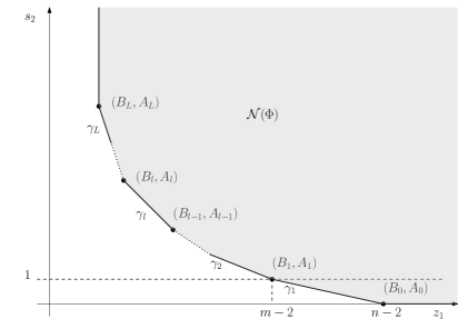
Figure 2. Edges

Notice also that

$$A_{l}+a_{l}B_{l}=A_{l-1}+a_{l}B_{l-1},$$

so that, if we put $\Delta A_{l}:=A_{l}-A_{l-1},\Delta B_{l}:=B_{l}-B_{l-1},$ then

$$a_{l}=\frac{\Delta A_{l}}{-\Delta B_{l}}$$

is just the (modulus) of the slope of the edge ${\gamma}_{l}:=[(B_{l},A_{l}),(B_{l-1},A_{l-1})]$ (compare Figure 2).

Let $L_{l}:=\{(t_{1},t_{2})\in{\mathbb{N}}^{2}:{\kappa}^{l}_{1}t_{1}+{\kappa}^{l}_{2}t_{2}=1\}$ denote the line supporting this edge ${\gamma}_{l}.$ It is easy to see that it is given by

$${\kappa}^{l}_{1} = \frac{\Delta A_{l}}{A_{l}\Delta B_{l}-B_{l}\Delta A_{l}}=\frac{a_{l}}{A_{l}+a_{l}B_{l}},$$

$${\kappa}^{l}_{2} = \frac{\Delta B_{l}}{A_{l}\Delta B_{l}-B_{l}\Delta A_{l}}=\frac{1}{A_{l}+a_{l}B_{l}}.$$

This defines a weight ${\kappa}^{l}:=({\kappa}_{1}^{l},{\kappa}_{2}^{l})$ associated to the edge ${\gamma}_{l},$ and we see that

$$\frac{{\kappa}^{l}_{1}}{{\kappa}^{l}_{2}}=a_{l}.$$

Note that

$$a_{1}<a_{2}<\dots<a_{l}<\dots<a_{L}.$$

Finally, fix $l,$ and let us determine the ${\kappa}^{l}$-principal part $\Phi_{{\kappa}^{l}}$ of $\Phi$ corresponding to the supporting line $L_{l}.$ To this end, observe that $\Phi$ has the same ${\kappa}^{l}$-principal part as the function

$$U_{0}(0,0)z_{1}^{\nu_{1}}\prod_{{\alpha},\mu}\Big{(}z_{1}-c^{\alpha}_{\mu}s_{2}^{a_{\mu}}\Big{)}^{N\left[\begin{matrix}{\alpha}\\ \mu\end{matrix}\right]}.$$

Moreover, the ${\kappa}^{l}$-principal part of $z_{1}-c^{\alpha}_{\mu}s_{2}^{a_{\mu}}$ is given by $-c^{\alpha}_{\mu}s_{2}^{a_{\mu}},$ if $\mu<l,$ and by $z_{1}$ if $\mu>l.$ This implies that

(6.12) $$\Phi_{{\kappa}^{l}}(z_{1},s_{2})=c_{l}\,s_{2}^{A_{l-1}}z_{1}^{B_{l}}\prod_{\alpha}\Big{(}z_{1}-c^{\alpha}_{l}s_{2}^{a_{l}}\Big{)}^{N{\left[\begin{matrix}{\alpha}\\ l\end{matrix}\right]}}.$$

In view of this identity, we shall say that the edge ${\gamma}_{l}$ is associated to the cluster of roots ${\left[\begin{matrix}\cdot\\ l\end{matrix}\right]}.$ We collect these results in the following lemma.

Lemma 6.2.

The vertices of the Newton polyhedron ${\mathcal{N}}(\Phi)$ of $\Phi$ are the points $(B_{l},A_{l}),$ $l=0,\dots,L,$ with $B_{j},A_{j}$ given by (6.10), and its compact edges are the intervals ${\gamma}_{l}:=[(B_{l},A_{l}),(B_{l-1},A_{l-1})],$ $l=1,\dots,L.$ Moreover the ${\kappa}^{l}$-principal part of $\Phi$ corresponding to the supporting line $L_{l}$ through the edge ${\gamma}_{l}$ is given by (6.12).

Based on the information given in this subsection and following ideas from [PS97], as well as from [IKM10] or [IM16], we shall apply a resolution (of singularity) algorithm which will allow us to reduce considerations step by step to suitable neighborhoods of smaller sub-clusters of roots until one ends up with a neighborhood a sub-cluster containing only one single root (with multiplicity)

7. Analysis in Step 1 of the resolution algorithm

We begin by working in our original coordinate $x_{1},$ and recall that we want to denote $x_{1}$ by $z_{1}.$ Recall also that we are restring attention to the upper half-plane $s_{2}>0.$

We shall decompose this half-plane into ${\kappa}^{l}$-homogeneous domains $D_{l}=D_{l}^{(1)}$ of the form

$$D_{l}:=\{(z_{1},s_{2}):2^{-M}s_{2}^{a_{l}}\leq|z_{1}|\leq 2^{M}s_{2}^{a_{l}}\},\quad l=1,\dots,L,$$

and transition domains

$$E_{0} := \{(z_{1},s_{2}):2^{M}s_{2}^{a_{1}}<|z_{1}|\},$$

$$E_{l} := \{(z_{1},s_{2}):2^{M}s_{2}^{a_{l+1}}<|z_{1}|<2^{-M}s_{2}^{a_{l}}\},\quad l=1,\dots,L-1,$$

$$E_{L} := \{(z_{1},s_{2}):|z_{1}|<2^{-M}s_{2}^{a_{L}}\}$$

between two such domains of different type of homogeneity. Here, $M\gg 1$ is an integer which will have to be chosen sufficiently large later on.

To localize to domains of type $D_{l}$ in a smooth way, we put more precisely

$$\rho_{l}(z_{1},s_{2}):=\chi_{0}\Big{(}\frac{z_{1}}{2^{M}s_{2}^{a_{l}}}\Big{)}-\chi_{0}\Big{(}\frac{z_{1}}{2^{-M}s_{2}^{a_{l}}}\Big{)},\quad l=1,\dots,L,$$

and replace $J({\lambda},s)$ in (6.4) by

$$J^{\rho_{l}}({\lambda},s):=\int e^{-i{\lambda}s_{3}(\breve{\phi}_{1}(z_{1},s_{2})+s_{1}z_{1})}\eta(z_{1},s_{2})\rho_{l}(z_{1},s_{2})\,dz_{1}.$$

The corresponding functions such as $\mu^{\lambda}$ and $F({\lambda},s_{2},s_{3},y_{1}),$ and the corresponding maximal operator will be designated by means an extra upper index $\rho_{l},$ such as $\mu^{\rho_{l},{\lambda}},$ $F^{\rho_{l}}({\lambda},s_{2},s_{3},y_{1})$ and ${\mathcal{M}}^{\rho_{l}}.$

Similarly, in order to localize to domains of type $E_{l},$ we put, for $l=1,\dots,L-1,$

$$\tau_{l}(z_{1},s_{2}) := \chi_{0}\Big{(}\frac{z_{1}}{2^{-M}s_{2}^{a_{l}}}\Big{)}\,-\chi_{0}\Big{(}\frac{z_{1}}{2^{M}s_{2}^{a_{l+1}}}\Big{)},$$

and define $\tau_{0}$ and $\tau_{L}$ by means of the obvious modifications of this definition. The corresponding functions and the corresponding maximal operator will be denoted by $\mu^{\tau_{l},{\lambda}},F^{\tau_{l}}({\lambda},s_{2},s_{3},y_{1}),{\mathcal{M}}^{\tau_{l}},$ … .

Recall that we may assume that $|s_{2}|<{\varepsilon},$ for any given ${\varepsilon}>0.$ It is then easy to see that, once we have chosen $M,$ by assuming that ${\varepsilon}>0$ is chosen sufficiently small, then $2^{-M}s_{2}^{a_{l}}>2^{M}s_{2}^{a_{l+1}}$ for every $l.$ Then the functions $\rho_{l},l=1,\dots L,$ jointly with the functions $\tau_{l},l=0,\dots L,$ form a partition of unity consisting of non-negative functions.

Finally note that it suffices to suitably control all the maximal operators defined in this way in order to prove the first statement in Theorem 1.2.

7.1. Dyadic localization in $z_{1}$ and $s_{2}$

Let us localize to

$$|z_{1}|\sim 2^{-j},\ s_{2}\sim 2^{-k},$$

where we may assume that $j,k$ are sufficiently large integers $\gg 1.$ To this end, we shall define scaled coordinates $z,{\sigma}_{2}$ by writing $z_{1}=2^{-j}z,\ s_{2}=2^{-k}{\sigma}_{2},$ so that

$$|z|\sim 1,\ s_{2}\sim 1.$$

Accordingly, let

$$J_{j,k}({\lambda},s) := \chi_{1}(2^{k}s_{2})\int e^{-i{\lambda}s_{3}(\breve{\phi}_{1}(z_{1},s_{2})+s_{1}z_{1})}\eta(z_{1},s_{2})\chi_{1}(2^{j}z_{1})\,dz_{1}$$

$$= \chi_{1}({\sigma}_{2})\,2^{-j}\int e^{-i{\lambda}s_{3}(\breve{\phi}_{1}(2^{-j}z,s_{2})+2^{-j}s_{1}z)}\chi_{1}(z)\,\eta(2^{-j}z,2^{-k}{\sigma}_{2})\,dz,$$

and

$$J^{\tau_{l}}_{j,k}({\lambda},s)=\chi_{1}({\sigma}_{2})\,2^{-j}\int e^{-i{\lambda}s_{3}(\breve{\phi}_{1}(2^{-j}z,s_{2})+2^{-j}s_{1}z)}\chi_{1}(z)\,(\tau_{l}\eta)(2^{-j}z,2^{-k}{\sigma}_{2})\,dz.$$

The corresponding functions such as $\mu^{\lambda}$ and $F({\lambda},s_{2},s_{3},y_{1}),$ and the corresponding maximal operator will be designated by means an extra lower index $j,k,$ such as $\mu^{{\lambda}}_{j,k},F_{j,k}({\lambda},s_{2},s_{3},y_{1}),{\mathcal{M}}_{j,k},$ and ${\mathcal{M}}^{\rho_{l}}_{j,k}.$

Convention: In order to defray the notation, we shall use the shorthand notation $\eta dz=\eta(2^{-j}z,2^{-k}{\sigma}_{2})\,dz$ in these integrals, as well as in many similar situations later on, where a smooth amplitude factor $\eta$ depending on integration variables (here the variable $z$) and small parameters (here $2^{-j}$ and $2^{-k}$) in such a way that we have uniform estimates for derivatives of these amplitude factors. The concrete meaning of $\eta$ will be allowed to be different at every instance where this symbol is used.

Thus, for instance we shall write

$$J^{\tau_{l}}_{j,k}({\lambda},s)=\chi_{1}({\sigma}_{2})\,2^{-j}\int e^{-i{\lambda}s_{3}(\breve{\phi}_{1}(2^{-j}z,s_{2})+2^{-j}s_{1}z)}\chi_{1}(z)\,\tau_{l}(2^{-j}z,2^{-k}{\sigma}_{2})\,\eta dz.$$

Similarly, we write

$$J^{\rho_{l}}_{j,k}({\lambda},s)=\chi_{1}({\sigma}_{2})\,2^{-j}\int e^{-i{\lambda}s_{3}(\breve{\phi}_{1}(2^{-j}z,s_{2})+2^{-j}s_{1}z)}\chi_{1}(z)\,\rho_{l}(2^{-j}z,2^{-k}{\sigma}_{2})\,\eta dz.$$

For the contribution by the transition domain $E_{l},$ i.e., for $J^{\tau_{l}},$ it is easily seen that we may assume that $J^{\tau_{l}}_{j,k}\equiv 0,$ unless

(7.1) $$j\geq ka_{l}+M/2,\qquad\text{if}\quad l=1,\dots L,$$

(7.2) $$j\leq ka_{l+1}-M/2,\qquad\text{if}\quad l=0,\dots L-1.$$

Similarly, for the contribution by the homogeneous domain $D_{l},1\leq l\leq L,$ i.e., for $J^{\rho_{l}},$ we may assume that $J^{\rho_{l}}_{j,k}\equiv 0,$ unless

(7.3) $$|j-ka_{l}|\leq M/2.$$

We thus see that the factors $\tau_{l}(2^{-j}z,2^{-k}{\sigma}_{2})$ respectively $\rho_{l}(2^{-j}z,2^{-k}{\sigma}_{2})$ can be absorbed into a modified factor $\eta$ in the definitions of $J^{\tau_{l}}_{j,k},$ respectively $J^{\rho_{l}}_{j,k},$ so that, with a slight abuse of notation, we may and shall henceforth assume that

$$J^{\tau_{l}}_{j,k}({\lambda},s) = J^{\rho_{l}}_{j,k}({\lambda},s)=J_{j,k}({\lambda},s)=\chi_{1}({\sigma}_{2})\,2^{-j}\int e^{-i{\lambda}s_{3}(\breve{\phi}_{1}(2^{-j}z,s_{2})+2^{-j}s_{1}z)}\chi_{1}(z)\,\eta dz$$

for the range of $j$s and $k$s described by (7.1) and (7.2), respectively (7.3).

7.2. Resolution of singularity on the transition domain $E_{l}$

It is well-known that on $E_{l},$ we may write

(7.4) $$\Phi(z_{1},s_{2})=V(z_{1},s_{2})\,s_{2}^{A_{l}}z_{1}^{B_{l}},\qquad(z_{1},s_{2})\in E_{l},$$

where the function $V$ is analytic away from the coordinate axes and $|V(z_{1},s_{2})|\sim 1$ (compare [PS97]). Actually, we shall need more precise information on the function $V:$ by (6.9), we may write

$$\Phi(z_{1},s_{2})=U_{0}(z_{1},s_{2})z_{1}^{\nu_{1}}\prod_{l^{\prime}=1}^{L}\prod_{r\in\left[\begin{matrix}\cdot\\ l^{\prime}\end{matrix}\right]}(z_{1}-r(s_{2})).$$

Now, if $l^{\prime}\geq l+1,$ then $a_{l^{\prime}}\geq a_{l+1},$ and since $a_{l^{\prime}}$ is the leading exponent of any root $r$ in the cluster $\left[\begin{matrix}\cdot\\ l^{\prime}\end{matrix}\right],$ we may factor

$$z_{1}-r(s_{2})=z_{1}\big{(}1-\frac{r(s_{2})}{z_{1}}\big{)},\quad\text{where}\ \frac{r(s_{2})}{z_{1}}=O(2^{-M/4}).$$

Similarly, if $l^{\prime}\leq l,$ then we may factor

$$z_{1}-r(s_{2})=s_{2}^{a_{l^{\prime}}}\big{(}-\frac{r(s_{2})}{s_{2}^{a_{l^{\prime}}}}+\frac{z_{1}}{s_{2}^{a_{l^{\prime}}}}\big{)},\quad\text{where}\ \frac{r(s_{2})}{s_{2}^{a_{l^{\prime}}}}=c^{\alpha}_{l^{\prime}}\neq 0,\text{ and }\frac{z_{1}}{s_{2}^{a_{l^{\prime}}}}=O(2^{-M/4}).$$

In combination with (6.10), this implies (7.4), with

$$V(z_{1},s_{2}):=U_{0}(z_{1},s_{2})\prod_{l^{\prime}=1}^{l}\prod_{r\in\left[\begin{matrix}\cdot\\ l^{\prime}\end{matrix}\right]}\big{(}-\frac{r(s_{2})}{s_{2}^{a_{l^{\prime}}}}+\frac{z_{1}}{s_{2}^{a_{l^{\prime}}}}\big{)}\prod_{l^{\prime}=l+1}^{L}\prod_{r\in\left[\begin{matrix}\cdot\\ l^{\prime}\end{matrix}\right]}\big{(}1-\frac{r(s_{2})}{z_{1}}\big{)}.$$

This implies in particular that, as a function of $z_{1},$ $V(z_{1},s_{2})$ admits a convergent Laurent expansion of the form

(7.5) $$V(z_{1},s_{2})=\sum\limits_{k=-B_{l}}^{\infty}z_{1}^{k}\rho_{k}(s_{2}),$$

where the $\rho_{k}(s_{2})$ are fractionally analytic in $s_{2}.$ Moreover, on $E_{l},$ we may assume that $|\rho_{0}(s_{2})|\sim 1$ and

$$\sum\limits_{0\neq k=-B_{l}}^{\infty}|z_{1}^{k}\rho_{k}(s_{2})|\ll 1.$$

In order derive information from (7.4) on the function $\Phi_{0}$ in (6.7), the following simple lemma will be useful:

Lemma 7.1.

Given $B\in{\mathbb{N}}$ and a smooth function $V(z)$ on an interval $I$ not containing $0,$ then there is a smooth function $U(z)$ on this interval such hat

$$\frac{d}{dz}\big{(}U(z)z^{B+1}\big{)}=V(z)z^{B}.$$

Proof.

We can choose

$$U(z):=z^{-(B+1)}\int z^{B}V(z)\,dz,$$

where the integral can designate any primitive of the integrand. Q.E.D.

Applying this to the term of order $k$ in (7.5), with $B=B_{l}$ and $B_{l}+k\geq 0,$ we see that if we define

$$V_{1}(z_{1},s_{2}):=\sum\limits_{k=-B_{l}}^{\infty}z_{1}^{k}\frac{\rho_{k}(s_{2})}{B_{l}+k+1},$$

then we find that

$${\partial}_{z_{1}}\big{(}V_{1}(z_{1},s_{2})z_{1}^{B_{l}+1}\big{)}=V(z_{1},s_{2})z_{1}^{B_{l}},$$

and iterating this once more, we obtain

$${\partial}_{z_{1}}^{2}\big{(}U(z_{1},s_{2})z_{1}^{B_{l}+2}\big{)}=V(z_{1},s_{2})z_{1}^{B_{l}},$$

if we set

$$U(z_{1},s_{2}):=\sum\limits_{k=-B_{l}}^{\infty}z_{1}^{k}\frac{\rho_{k}(s_{2})}{(B_{l}+k+1)(B_{l}+k+2)}.$$

Consequently,

$${\partial}_{z_{1}}^{2}\big{(}U(z_{1},s_{2})s_{2}^{A_{l}}z_{1}^{B_{l}+2}\big{)}=\Phi(z_{1},s_{2})={\partial}_{z_{1}}^{2}\breve{\phi}_{1}(z_{1},s_{2}).$$

Clearly, $U(z_{1},s_{2})$ has similar properties as $V(z_{1},s_{2});$ in particular, $|U(z_{1},s_{2})|\sim 1.$ Note also that the function $U(z_{1},s_{2})s_{2}^{A_{l}}z_{1}^{B_{l}+2}$ is analytic in $z_{1}$ and vanishes of second order at $z_{1}=0.$ Consequently, we see that

$$\breve{\phi}_{1}(z_{1},s_{2})=U(z_{1},s_{2})s_{2}^{A_{l}}z_{1}^{B_{l}+2}+z_{1}g(s_{2})+h(s_{2}),$$

where

$$\begin{split}h(s_{2})&=\breve{\phi}_{1}(0,s_{2})\equiv 0,\\ g(s_{2})&={\partial}_{z_{1}}\breve{\phi}_{1}(0,s_{2})=s_{2}^{2}q(0,s_{2})=:s_{2}^{2}q_{0}(s_{2}).\end{split}$$

Thus, we find that, on $E_{l},$

(7.6) $$\Phi_{0}(z_{1},s^{\prime}):=\breve{\phi}_{1}(z_{1},s_{2})+s_{1}z_{1}=U(z_{1},s_{2})s_{2}^{A_{l}}z_{1}^{B_{l}+2}+z_{1}(s_{1}+s^{2}q_{0}(s_{2})).$$

Let us finally again apply our changes of coordinates $z_{1}=2^{-j}z,\ s_{2}=2^{-k}{\sigma}_{2}.$ Then, if we put $A:=A_{l},B:=B_{l}$ and

$$d_{j,k}:=2^{-kA-j(B+2)},$$

assuming that (7.1), (7.2) hold true, we have that

(7.7) $$\Phi_{0}^{s}(z,s_{1},{\sigma}_{2}):=\Phi_{0}(z_{1},s^{\prime})=U^{s}(z,{\sigma}_{2})\,d_{j,k}{\sigma}_{2}^{A}z^{B+2}+2^{-j}z\big{(}s_{1}+2^{-2k}{\sigma}_{2}^{2}g^{s}({\sigma}_{2})\big{)},$$

with $U^{s}(z,{\sigma}_{2}):=U(2^{-j}z,2^{-k}{\sigma}_{2})$ and $g^{s}({\sigma}_{2}):=q_{0}(2^{-k}{\sigma}_{2}).$ Note that $|U^{s}(z,{\sigma}_{2})|\sim 1,$ whereas derivatives of $U^{s}(z,{\sigma}_{2})$ can be assumed to be very small, and recall that

$$|z|\sim 1,\sigma_{2}\sim 1,|s_{1}|\ll 1.$$

Note also that

(7.8) $$d_{j,k}\leq 2^{-2j}\ll 2^{-j}.$$

7.3. $L^{2}$ - estimation of ${\mathcal{M}}_{j,k}^{\lambda}$ for the contribution by $E_{l}$

We begin by observing that since $d_{j,k}\ll 2^{-j},$ by choosing $s_{1}$ and $s_{2}$ properly we can always find a critical point of $\Phi_{0}^{s}$ in (7.7) w.r. to $z.$ Thus, in view of Plancherel’s theorem, the best possible estimate of ${\mathcal{M}}_{j,k}^{\lambda}$ can be achieved by means of an application of van der Corput’s estimate of order $2$ to

$$J_{j,k}({\lambda},s)=\chi_{1}({\sigma}_{2})\,2^{-j}\int e^{-i{\lambda}s_{3}\Phi_{0}^{s}(z,s_{1},{\sigma}_{2})}\chi_{1}(z)\,\eta dz.$$

This leads to $|J_{j,k}({\lambda},s)|\lesssim 2^{-j}({\lambda}d_{j,k})^{-1/2},$ if ${\lambda}d_{j,k}\geq 1.$ If ${\lambda}d_{j,k}\leq 1,$ the trivial estimate $|J_{j,k}({\lambda},s)|\lesssim 2^{-j}$ holds true. Since, by (6.3), $|\widehat{\mu^{\lambda}_{j,k}}|\lesssim{\lambda}^{-1/2}|J_{j,k}({\lambda},s)|,$ the usual arguments show that this implies the following $L^{2}$- estimate:

(7.9) $$\|{\mathcal{M}}^{\lambda}_{j,k}\|_{2\to 2}\lesssim 2^{-j}(1+{\lambda}d_{j,k})^{-\frac{1}{2}}.$$

Remark 7.2.

Throughout Section 7, we shall assume that ${\lambda}2^{-j}\geq 1,$ i.e., $j\lesssim\log{\lambda}.$ The case where ${\lambda}2^{-j}\geq 1$ will be discussed in Subsection 8.7 of Section 8.

7.4. $L^{1+{\varepsilon}}$ - estimates of ${\mathcal{M}}_{j,k}^{\lambda}$ for the contribution by $E_{l},l=1,\dots,L,$ when ${\lambda}\geq 2^{j}$

In view of Lemma 5.4, the $L^{1+{\varepsilon}}$ - estimates require pointwise bounds for $\mu_{j,k}^{\lambda}.$ By (6.5), we have

$$\mu_{j,k}^{\lambda}(y+{\Gamma})={\lambda}^{\frac{5}{2}}2^{-k}\int\int F_{j,k}({\lambda},2^{-k}{\sigma}_{2},s_{3},y_{1})e^{-i{\lambda}s_{3}(s_{2}^{2}B(s_{2})-2^{-k}{\sigma}_{2}y_{2}-y_{3})}\chi_{1}({\sigma}_{2})d{\sigma}_{2}\chi_{1}(s_{3})ds_{3},$$

where

$$F_{j,k}({\lambda},2^{-k}{\sigma}_{2},s_{3},y_{1}) = 2^{-j}\iint e^{-i{\lambda}s_{3}(\Phi_{0}^{s}(z,s_{1},{\sigma}_{2})-s_{1}y_{1})}\chi_{0}(s_{1})\chi_{1}(z)\,\eta dzds_{1}.$$

Let us put $Y_{1}:=2^{j}y_{1},$ and use (7.6) to write the phase function in the latter integral as

(7.10) $$\Phi_{0}^{s}(z,s_{1},{\sigma}_{2})-s_{1}y_{1}=2^{-j}\big{[}U^{s}(z,{\sigma}_{2})\,2^{j}d_{j,k}{\sigma}_{2}^{A}z^{B+2}+z2^{-2k}{\sigma}_{2}^{2}g^{s}({\sigma}_{2})+s_{1}(z-Y_{1})\big{]}$$

Let us first consider the contribution by the region where $|Y_{1}|\gg 1$ and $|Y_{1}|\geq{\lambda}^{{\delta}-1}2^{j},$ where we assume that $0<{\delta}\ll 1.$ Here, ${\lambda}2^{-j}|Y_{1}|\gg{\lambda}^{\delta},$ and since $|z|\sim 1,$ integrations by parts in $s_{1}$ show that $F_{j,k}({\lambda},2^{-k}{\sigma}_{2},s_{3},y_{1})=O({\lambda}^{-N})$ for every $N\in{\mathbb{N}},$ and thus also $\mu_{j,k}^{\lambda}(y+{\Gamma})=O({\lambda}^{-N})$ for every $N\in{\mathbb{N}},$ which shows that this leads just to a small error term.

Consider next the contribution by the region where $1\ll|Y_{1}|\leq{\lambda}^{{\delta}-1}2^{j}.$ Then, by (7.8),

$${\lambda}d_{j,k}\leq 2^{\frac{j}{1-{\delta}}}2^{-2j}\ll 1,$$

if we choose ${\delta}$ sufficiently small. This shows that we can include the exponential factor corresponding to the term $U^{s}(z,{\sigma}_{2})\,d_{j,k}{\sigma}_{2}^{A}z^{B+2}$ of the phase $\Phi_{0}^{s}$ into the amplitude and consequently ignore it. Let us then collect all summands of the complete phase in the oscillatory integral $\mu_{j,k}^{\lambda}(y+{\Gamma})$ which depend on ${\sigma}_{2}:$

(7.11) $$\begin{split}&2^{-j}z2^{-2k}{\sigma}_{2}^{2}\tilde{g}({\sigma}_{2}))+2^{-2k}{\sigma}_{2}^{2}B(2^{-k}{\sigma}_{2})-2^{-k}{\sigma}_{2}y_{2}\\ &=2^{-2k}\big{[}{\sigma}_{2}^{2}B(2^{-k}{\sigma}_{2})-{\sigma}_{2}Y_{2}+2^{-j}{\sigma}_{2}^{2}z\tilde{g}({\sigma}_{2})\big{]},\end{split}$$

where we have set $Y_{2}:=2^{k}y_{2}.$

Let us now decompose the region where $1\ll|Y_{1}|\leq{\lambda}^{{\delta}-1}2^{j}$ into the regions

$$\Delta_{\iota_{1}}:=\{y:|Y_{1}|\sim 2^{\iota_{1}}\},$$

where clearly we may assume that $1\ll\iota_{1}<j.$ We further decompose $\Delta_{\iota_{1}}$ into the subregions

$$\Delta_{\iota_{1},\iota_{2}} := \{y:|Y_{1}|\sim 2^{\iota_{1}},|Y_{2}|\sim 2^{\iota_{2}}\},\quad 1\ll\iota_{2}\leq k,$$

$$\Delta_{\iota_{1},0} := \{y:|Y_{1}|\sim 2^{\iota_{1}},|Y_{2}|\lesssim 1\}.$$

Then

$$|\Delta_{\iota_{1},\iota_{2}}|\lesssim 2^{\iota_{1}+\iota_{2}-j-k}.$$

The corresponding measures which are given by restricting $\mu_{j,k}^{\lambda}$ to the corresponding sets and the associated maximal operators will be denoted $\mu_{k,j,\iota}^{\lambda}$ and ${\mathcal{M}}_{j,k,\iota}^{\lambda}.$

Now, clearly, if $y\in\Delta_{\iota_{1}},$ then we may integrate by parts in $s_{1}.$

Moreover, if $\iota_{2}\gg 1,$ and if ${\lambda}2^{-2k+\iota_{2}}\geq 1,$ then (7.11) shows that we can also integrate by parts in ${\sigma}_{2},$ and altogether this leads to the following estimate for $\mu_{k,j,\iota}^{\lambda}:$

$$|\mu_{j,k,\iota}^{\lambda}(y+{\Gamma})|\lesssim{\lambda}^{\frac{5}{2}}2^{-j-k}({\lambda}2^{-j}2^{\iota_{1}})^{-1}({\lambda}2^{-2k}2^{\iota_{2}})^{-1}={\lambda}^{\frac{1}{2}}2^{k-\iota_{1}-\iota_{2}}.$$

Thus, Lemma 5.4 shows that, for every ${\varepsilon}>0,$

$$\|{\mathcal{M}}_{j,k,\iota}^{\lambda}\|_{1+{\varepsilon}\to 1+{\varepsilon}}\lesssim{\lambda}^{\frac{1}{2}}2^{-j}.$$

But, recall that we are assuming that $j\lesssim\log{\lambda},$ and note that ${\lambda}2^{-2k+\iota_{2}}\geq 1$ implies that ${\lambda}2^{-k}\geq 1,$ hence $\iota_{2}\leq k\lesssim\log{\lambda},$ so that by summing over these $\iota$s we will just pick up an extra factor $(\log{\lambda})^{2}$ compared to previous estimate:

(7.12) $$\sum\limits_{\iota_{1}\lesssim j,\iota_{2}\leq k}\|{\mathcal{M}}_{j,k,\iota}^{\lambda}\|_{1+{\varepsilon}\to 1+{\varepsilon}}\lesssim{\lambda}^{\frac{1}{2}+{\varepsilon}}2^{-j},$$

for every ${\varepsilon}>0.$

Assume next that $\iota_{2}\gg 1$ and ${\lambda}2^{-2k+\iota_{2}}<1.$ Then $1\ll 2^{\iota_{2}}<2^{2k}{\lambda}^{-1},$ and so we cannot gain anything from the integration in ${\sigma}_{2}$ and arrive at the following estimate:

$$|\mu_{j,k,\iota}^{\lambda}(y+{\Gamma})|\lesssim{\lambda}^{\frac{5}{2}}2^{-j-k}({\lambda}2^{-j}2^{\iota_{1}})^{-1}={\lambda}^{\frac{3}{2}}2^{-k-\iota_{1}},$$

hence $\|{\mathcal{M}}_{j,k,\iota}^{\lambda}\|_{1+{\varepsilon}\to 1+{\varepsilon}}\lesssim{\lambda}^{\frac{3}{2}}2^{-j+\iota_{2}-2k}.$ Thus, summing over the corresponding $\iota$s, we get

$$\sum\limits_{\iota_{1}\lesssim j,\,2^{\iota_{2}}<2^{2k}{\lambda}^{-1}}\|{\mathcal{M}}_{j,k,\iota}^{\lambda}\|_{1+{\varepsilon}\to 1+{\varepsilon}}\lesssim\sum\limits_{\iota_{1}\lesssim j,\,2^{\iota_{2}}<2^{2k}{\lambda}^{-1}}{\lambda}^{\frac{3}{2}}2^{-j+\iota_{2}-2k}<{\lambda}^{\frac{1}{2}+{\varepsilon}}2^{-j},$$

which matches with (7.12).

Assume finally that $\iota_{2}=0.$ Then, in place of an integration by parts in ${\sigma}_{2},$ we apply van der Corput’s estimate of order 2 in ${\sigma}_{2},$ which leads to

$$|\mu_{j,k,\iota}^{\lambda}(y+{\Gamma})|\lesssim{\lambda}^{\frac{5}{2}}2^{-j-k}({\lambda}2^{-j}2^{\iota_{1}})^{-1}({\lambda}2^{-2k})^{-\frac{1}{2}}={\lambda}2^{-\iota_{1}},$$

hence

(7.13) $$\|{\mathcal{M}}_{j,k,(\iota_{1},0)}^{\lambda}\|_{1+{\varepsilon}\to 1+{\varepsilon}}\lesssim{\lambda}^{1+{\varepsilon}}2^{-j-k}.$$

Again, we can sum in $\iota_{1}\lesssim j,$ and combining all our estimates we see that the contribution ${\mathcal{M}}_{j,k,|Y_{1}|\gg 1}^{\lambda}$ of the region where $|Y_{1}|\gg 1$ to ${\mathcal{M}}_{j,k}^{\lambda}$ can be estimated by

(7.14) $$\|{\mathcal{M}}_{j,k,|Y_{1}|\gg 1}^{\lambda}\|_{1+{\varepsilon}\to 1+{\varepsilon}}\lesssim{\lambda}^{\frac{1}{2}+{\varepsilon}}2^{-j}+{\lambda}^{1+{\varepsilon}}2^{-j-k},$$

for every ${\varepsilon}>0.$

What remains is the contribution ${\mathcal{M}}_{j,k,|Y_{1}|\lesssim 1}^{\lambda}$ of the region where $|Y_{1}|\lesssim 1$ to ${\mathcal{M}}_{j,k}^{\lambda}.$ A look at the phase (7.10) shows that we are now in the position to apply Lemma 5.2 to the oscillatory integral $F_{j,k}({\lambda},2^{-k}{\sigma}_{2},s_{3},y_{1})$ in the variables $(s_{1},z)$ in place of $(\eta,x),$ with $N:={\lambda}2^{-j}\geq 1.$ Moreover, observe that $s_{1}$ and $z$ result from our original coordinates $s_{1}$ and $z_{1}=x_{1}$ by means of a smooth change of coordinates. Passing back to our original coordinate, according to Remarks 5.3 we therefore must evaluate the original phase $\breve{\phi}_{1}(x_{1},s_{2})+s_{1}x_{1}-s_{1}y_{1}$ in (6.6) at $x_{1}=y_{1},$ and thus get

(7.15) $$F_{j,k,|Y_{1}|\lesssim 1}({\lambda},s_{2},s_{3},y_{1})=({\lambda}2^{-j})^{-1}2^{-j}e^{-i{\lambda}s_{3}(\breve{\phi}_{1}(y_{1},s_{2})}\eta(y_{1},2^{-k}{\sigma}_{2}).$$

This implies that

$$\mu_{j,k,|Y_{1}|\lesssim 1}^{\lambda}(y+{\Gamma})={\lambda}^{\frac{3}{2}}2^{-k}\int e^{-i{\lambda}s_{3}\big{(}\breve{\phi}_{1}(y_{1},2^{-k}{\sigma}_{2})+2^{-2k}{\sigma}_{2}^{2}B(2^{-k}{\sigma}_{2})-2^{-k}{\sigma}_{2}y_{2}-y_{3}\big{)}}\chi_{1}({\sigma}_{2})\chi_{1}(s_{3})\,\eta d{\sigma}_{2}ds_{3}.$$

By (6.2), the complete phase is here given by

$$2^{-2k}\big{[}{\sigma}_{2}^{2}B(2^{-k}{\sigma}_{2})+y_{1}{\sigma}_{2}^{2}q(y_{1},2^{-k}{\sigma}_{2})-2^{k}{\sigma}_{2}(y_{2}-y_{1}^{m}\omega(y_{1}))\big{]}+y_{1}^{n}\beta(y_{1})-y_{3}.$$

In order to estimate the result of the integration in ${\sigma}_{2},$ we can argue now in a similar way as before and decompose the region where $|Y_{1}|\lesssim 1$ into the subregions

$$\Delta_{\iota_{2}} := \{y:|Y_{1}|\lesssim 1,2^{k}|y_{2}-y_{1}^{m}\omega(y_{1})|\sim 2^{\iota_{2}}\},1\ll\iota_{2}\leq k,$$

$$\Delta_{0} := \{y:|Y_{1}|\lesssim 1,2^{k}|y_{2}-y_{1}^{m}\omega(y_{1})|\lesssim 1\}.$$

Then

$$|\Delta_{\iota_{2}}|\lesssim 2^{-j}2^{\iota_{2}-k}.$$

If $\iota_{2}\gg 1,$ then we may integrate by parts in ${\sigma}_{2}$ and obtain

$$|\mu_{j,k,|Y_{1}|\lesssim 1,\iota_{2}}^{\lambda}(y+{\Gamma})|\lesssim{\lambda}^{\frac{3}{2}}2^{-k}({\lambda}2^{-2k+\iota_{2}})^{-1}={\lambda}^{\frac{1}{2}}2^{k-\iota_{2}},$$

hence

$$\|{\mathcal{M}}_{j,k,|Y_{1}|\lesssim 1,\iota_{2}}^{\lambda}\|_{1+{\varepsilon}\to 1+{\varepsilon}}\lesssim{\lambda}^{\frac{1}{2}}2^{-j}.$$

And, if $\iota_{2}=0,$ then we apply van der Corput’s estimate of order 2 in ${\sigma}_{2},$ which leads to

$$|\mu_{j,k,|Y_{1}|\lesssim 1,\iota_{2}}^{\lambda}(y+{\Gamma})|\lesssim{\lambda}^{\frac{3}{2}}2^{-k}({\lambda}2^{-2k})^{-\frac{1}{2}}={\lambda},$$

hence

$$\|{\mathcal{M}}_{j,k,|Y_{1}|\lesssim 1,\iota_{2}}^{\lambda}\|_{1+{\varepsilon}\to 1+{\varepsilon}}\lesssim{\lambda}2^{-k}2^{-j}.$$

These estimates match with (7.14), and thus altogether we find that, for every ${\varepsilon}>0,$

(7.16) $$\|{\mathcal{M}}_{j,k}^{\lambda}\|_{1+{\varepsilon}\to 1+{\varepsilon}}\lesssim{\lambda}^{1+{\varepsilon}}2^{-j-k}+{\lambda}^{\frac{1}{2}+{\varepsilon}}2^{-j}.$$

7.5. $L^{p}$ - estimates of ${\mathcal{M}}_{j,k}^{\lambda}$ for the contribution by $E_{l}$ when ${\lambda}\geq 2^{j}$

Interpolation between the $L^{2}$ - estimate (7.9) and the $L^{1+{\varepsilon}}$ - estimate (7.16) leads to

(7.17) $$\|{\mathcal{M}}_{j,k}^{\lambda}\|_{p\to p} \lesssim ({\lambda}^{1+{\varepsilon}}2^{-k})^{\frac{2}{p}-1}(1+{\lambda}d_{j,k})^{-\frac{1}{2}(2-\frac{2}{p})}2^{-j}+({\lambda}^{\frac{1}{2}+{\varepsilon}})^{\frac{2}{p}-1}(1+{\lambda}d_{j,k})^{-\frac{1}{2}(2-\frac{2}{p})}2^{-j}$$

$$\lesssim {\lambda}^{{\varepsilon}^{\prime}}({\lambda}d_{j,k})^{\frac{2}{p}-1}(1+{\lambda}d_{j,k})^{\frac{1}{p}-1}\,(d_{j,k}^{-1})^{\frac{2}{p}-1}\,2^{-k(\frac{2}{p}-1)}\,2^{-j}$$

$$\quad+\,{\lambda}^{{\varepsilon}^{\prime}}({\lambda}d_{j,k})^{\frac{1}{p}-\frac{1}{2}}(1+{\lambda}d_{j,k})^{\frac{1}{p}-1}\,(d_{j,k}^{-1})^{\frac{1}{p}-\frac{1}{2}}\,2^{-j},$$

if $1<p<2.$

• Since $1/p-1/2>0,$ we can first sum both terms over all dyadic ${\lambda}$s such that ${\lambda}d_{j,k}\leq 1,$ provided we choose ${\varepsilon}^{\prime}>0$ sufficiently small.

• If ${\lambda}d_{j,k}>1,$ then the total exponent of ${\lambda}d_{j,k}$ in the first summand is

  $$\frac{2}{p}-1+\frac{1}{p}-1=\frac{3}{p}-2<0,$$

  since we are assuming that $p>3/2.$ Similarly, the total exponent of ${\lambda}d_{j,k}$ in the second summand is

  $$\frac{1}{p}-\frac{1}{2}+\frac{1}{p}-1=\frac{2}{p}-\frac{3}{2}<\frac{4}{3}-\frac{3}{2}<0.$$

  Thus, again both terms can be summed over all dyadic ${\lambda}$s such that ${\lambda}d_{j,k}>1,$ provided we choose ${\varepsilon}^{\prime}>0$ sufficiently small.

This easily shows that, for every ${\varepsilon}^{\prime}>0,$

(7.18) $$\sum\limits_{{\lambda}\gg 1}\|{\mathcal{M}}_{j,k}^{\lambda}\|_{p\to p}\lesssim(d_{j,k}^{-1})^{\frac{2}{p}-1+{\varepsilon}^{\prime}}\,2^{-k(\frac{2}{p}-1)}\,2^{-j}+(d_{j,k}^{-1})^{\frac{1}{p}-\frac{1}{2}+{\varepsilon}^{\prime}}\,2^{-j}.$$

In order to also sum over the $j$s and $k$s associated to $E_{l},$ it turns out that we shall have to make use of the condition (7.1). To this end, we shall first derive a little lemma which will help to relate any edge of ${\mathcal{N}}(\Phi)$ having the vertex $(B,A):=(B_{l},A_{l})$ associated to the transition domain $E_{l}$ as an endpoint.

7.6. A geometric lemma and $L^{p}$-estimation of ${\mathcal{M}}^{\tau_{l}},l=1,\dots,L$

Lemma 7.3.

Given a weight ${\kappa}=({\kappa}_{1},{\kappa}_{2})$ such that ${\kappa}_{1}>0,{\kappa}_{2}\geq 0,$ and the associated line

$$L_{\kappa}:=\{(t_{1},t_{2}):{\kappa}_{1}t_{1}+{\kappa}_{2}t_{2}=1\},$$

assume that $(B,A)$ is any point on $L_{\kappa}.$ We define the number $n_{\kappa}-2$ as the $t_{1}$-coordinate of the intersection of the line $L_{\kappa}$ with the horizontal line $t_{2}=1$ (compare Figure 4). Then

$$n_{\kappa}=\frac{A-1}{a}+B+2,$$

where $a:={\kappa}_{1}/{\kappa}_{2}$ is the modulus of the slope of the line $L_{\kappa}.$

Proof.

The condition ${\kappa}_{1}B+{\kappa}_{2}A=1$ is equivalent to $A/a+B=1/{\kappa}_{1},$ hence to

$$\frac{A-1}{a}+B+2=\frac{1}{{\kappa}_{1}}-\frac{{\kappa}_{2}}{{\kappa}_{1}}+2=\frac{1-{\kappa}_{2}}{{\kappa}_{1}}+2=(n_{\kappa}-2)+2=n_{\kappa}.$$

Q.E.D.

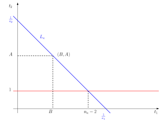
Figure 4. Meaning of $n_{\kappa}$

The next lemma will allow us to show that the estimates in (7.18) can be summed over the relevant $j$s and $k$s. Since in Step 2 and higher we shall have to deal with functions $\Phi(z,s_{2})$ which are analytic in the first variable $z,$ but only fractionally analytic in the second variable, we shall state it more generally for Newton-Puiseux polyhedra.

So, assume that $\Phi$ is such a function, with Newton-Puiseux polyhedron ${\mathcal{N}}(\Phi),$ whose vertices are the points $(B_{l},A_{l}),l=0,\dots L,$ where $(B_{0},A_{0})=(n-2,0),$ somewhat as in Subsection 6.2 (compare Figure 2). Note, however, that in contrast to the case of Newton polyhedra, where necessarily $A_{1}\geq 1,$ we may possibly have $A_{1}<1.$ Otherwise, we adapt the same notation as in Subsection 6.2.

Lemma 7.4.

Assume that $A_{1}\geq 1,$ so that $A_{l}\geq 1$ for every $l\geq 1.$ Then

$$\frac{A_{l}-1}{a_{l}}+B_{l}+2\leq\frac{A_{1}-1}{a_{1}}+B_{1}+2=\frac{A_{0}-1}{a_{1}}+B_{0}+2$$

for $l=1,\dots,L.$

The proof is geometrically evident in view of Lemma 7.3 (note that apparently the sequence $\{n_{{\kappa}^{l}}\}_{l}$ is decreasing) and can easily by carried out by means of an induction over $l\geq 0.$ It will therefore be omitted.

We are now in the position to show that the estimates in (7.18) can be summed over all relevant $j$s and $k$s associated to a given transition domain $E_{l},l=1,\dots,L,$ provided $p>\max\{3/2,h\}.$ Actually, we shall only need condition (7.1) here, i.e., $j\geq ka_{l}+M/2.$ Indeed, we shall prove that under these assumptions

(7.19) $$\sum\limits_{j,k\gg 1:j\geq ka_{l}}\Big{(}(d_{j,k}^{-1}2^{-k})^{\frac{2}{p}-1+{\varepsilon}^{\prime}}\,2^{-j}+(d_{j,k}^{-1})^{\frac{1}{p}-\frac{1}{2}+{\varepsilon}^{\prime}}\,2^{-j}\Big{)}<\infty,$$

provided we choose ${\varepsilon}^{\prime}>0$ sufficiently small.

In combination with estimate (7.18) this will clearly imply that for if $l=1,\dots,L,$

(7.20) $$\|{\mathcal{M}}^{\tau_{l}}\|_{p\to p}<\infty,$$

provided $p>\max\{3/2,h\}.$

Now, from (6.2) and (6.8), we find that the first two vertices of ${\mathcal{N}}(\Phi)$ are given by $(B_{0},A_{0})=(n-2,0)$ and $(B_{1},A_{1})=(m-2,1),$ and that ${\kappa}_{1}^{1}=1/(n-2)>0$ and

$$a_{1}=\frac{{\kappa}_{1}^{1}}{{\kappa}^{1}_{2}}=\frac{1}{n-m}.$$

(compare also Figure 2). Thus, Lemma 7.4 implies that

(7.21) $$\frac{A_{l}-1}{a_{l}}+B_{l}+2\leq m$$

for $l=1,\dots,L.$ Fix such an $l,$ and put $A:=A_{l},B:=B_{l}$ and $a=a_{l}>a_{1}=1/(n-m)>0.$ Then $d_{j,k}^{-1}=2^{kA+j(B+2)}$ and $k\leq j/a$ in (7.19). Thus, we can re-write (7.19) as

(7.22) $$\sum\limits_{j,k\gg 1:k\leq j/a}\Big{(}(2^{k(A-1)+j(B+2)})^{\frac{2}{p}-1+{\varepsilon}^{\prime}}\,2^{-j}+(2^{kA+j(B+2)})^{\frac{1}{p}-\frac{1}{2}+{\varepsilon}^{\prime}}\,2^{-j}\Big{)}<\infty.$$

Since the exponents $\frac{2}{p}-1+{\varepsilon}^{\prime}$ and $\frac{1}{p}-\frac{1}{2}+{\varepsilon}^{\prime}$ are strictly positive, we can first sum over all $k\leq j/a$ and are left with showing that

$$\sum\limits_{j\gg 1}\Big{(}2^{j\big{[}(\frac{A-1}{a}+B+2)(\frac{2}{p}-1+{\varepsilon}^{\prime})-1\big{]}}+2^{j\big{[}\frac{A}{a}+B+2)(\frac{1}{p}-\frac{1}{2}+{\varepsilon}^{\prime})-1\big{]}}\Big{)}<\infty.$$

But, by (7.21),

$$\frac{A-1}{a}+B+2\leq m\quad\text{and}\quad\frac{2}{p}-1<\frac{2}{n}\leq\frac{1}{m},$$

since $1/p<1/h=1/2+1/n$ and $n\geq 2m,$ so that we may assume that the exponent of the first summand in (7.22) is strictly negative and we can sum in $j.$

Similarly,

$$\frac{A}{a}+B+2\leq m+\frac{1}{a}\leq m+(n-m)=n\quad\text{and}\quad\frac{1}{p}-\frac{1}{2}<\frac{1}{n},$$

so that we may assume that the exponent of the second summand in (7.22) is strictly negative too and we can again sum in $j.$ This completes the proof of (7.19).

7.7. $L^{p}$-estimation of ${\mathcal{M}}^{\tau_{0}}$

Let us finally look at the case $l=0.$ Recall that here only the condition (7.2), i.e., $j\leq ka_{1}-M/2,$ is available, and that now

$$d_{j,k}^{-1}=2^{kA_{0}+j(B_{0}+2)}=2^{jn}.$$

Thus, here we would like to show that

(7.23) $$\sum\limits_{j,k\gg 1:k\geq j/a_{1}}\Big{(}(2^{jn-k})^{\frac{2}{p}-1+{\varepsilon}^{\prime}}\,2^{-j}+(2^{jn})^{\frac{1}{p}-\frac{1}{2}+{\varepsilon}^{\prime}}\,2^{-j}\Big{)}<\infty.$$

In the first summand, we can first sum over all $k\geq j/a_{1}$ and arrive at the sum

$$\sum\limits_{j\gg 1}2^{j\big{[}(n-\frac{1}{a_{1}})(\frac{2}{p}-1+{\varepsilon}^{\prime})-1\big{]}}.$$

But,

$$n-\frac{1}{a_{1}}=m,\quad\text{and}\quad\frac{2}{p}-1<\frac{2}{n}\leq\frac{1}{m},$$

so that we may assume that the exponent of the first summand in (7.23) is strictly negative by choosing ${\varepsilon}^{\prime}$ sufficiently small, and thus we can sum in $j.$

The second summand is insufficient for a summation in $k,$ unless, say, $k\lesssim j.$ In the latter case, we can sum in $k\lesssim j$ and arrive at the sum

(7.24) $$\sum\limits_{j\gg 1}2^{jn(\frac{1}{p}-\frac{1}{2}+{\varepsilon}^{\prime})}\,2^{-j},$$

with any slightly bigger ${\varepsilon}^{\prime}>0$ than before. This series is convergent for ${\varepsilon}^{\prime}$ sufficiently small, since we are assuming that $p>h.$

So, let us assume henceforth that, say, $k>jn.$ The crucial observation is that the second term in (7.16) can be improved when ${\lambda}2^{-k}\leq 1,$ and this will be needed for the case $l=0.$

To be more precise, assume first that ${\lambda}2^{-k}>1,$ i.e., $k\lesssim\log{\lambda}.$ Then we can keep the second term in (7.17), which is here given by

$${\lambda}^{{\varepsilon}^{\prime}}({\lambda}2^{-jn})^{\frac{1}{p}-\frac{1}{2}}(1+{\lambda}2^{-jn})^{\frac{1}{p}-1}\,(2^{jn})^{\frac{1}{p}-\frac{1}{2}}\,2^{-j}.$$

Summing now first in $k\lesssim\log{\lambda},$ we can estimate by the same kind of expression, but with a slightly bigger exponent ${\varepsilon}^{\prime}>0.$ After summing in ${\lambda},$ we are again left with the series in (7.24) and are done.

Assume next that ${\lambda}2^{-k}\leq 1.$ Then the exponential factor of the oscillatory integral $\mu_{j,k}^{\lambda}(y+\Gamma)$ which collects all terms depending only on ${\sigma}_{2}$ (compare (7.11)) is essentially non-oscillatory, and so we shall rather estimate for $y\in\Delta_{\iota_{1}}$ by

$$|\mu_{j,k,\iota_{1}}^{\lambda}(y+{\Gamma})|\lesssim{\lambda}^{\frac{5}{2}}2^{-j-k}({\lambda}2^{-j}2^{\iota_{1}})^{-1}={\lambda}^{\frac{3}{2}}2^{-k-\iota_{1}}.$$

Since $|\Delta_{\iota_{1}}|\lesssim 2^{\iota_{1}-j},$ we obtain the improved estimate

$$\|{\mathcal{M}}_{j,k,\iota_{1}}^{\lambda}\|_{1+{\varepsilon}\to 1+{\varepsilon}}\lesssim{\lambda}^{\frac{3}{2}}2^{-j-k}.$$

This shows that we can replace the second term in (7.16) by ${\lambda}^{\frac{3}{2}+{\varepsilon}}2^{-j-k},$ and finally, after interpolation with our $L^{2}$-estimate (7.9), we are led to summing

$$M({\lambda},j,k):=({\lambda}^{\frac{3}{2}+{\varepsilon}}2^{-k})^{\frac{2}{p}-1}(1+{\lambda}2^{-jn})^{\frac{1}{p}-1}2^{-j}$$

over our ${\lambda}$s, $j$s and $k$s.

Assume first that $2^{k}\geq{\lambda}>2^{jn}.$ Then $M({\lambda},j,k)\sim({\lambda}^{\frac{3}{2}+{\varepsilon}}2^{-k})^{\frac{2}{p}-1}({\lambda}2^{-jn})^{\frac{1}{p}-1}2^{-j},$ hence

$$\sum\limits_{k:2^{k}\geq{\lambda}}M({\lambda},j,k) \lesssim {\lambda}^{\frac{1}{p}-\frac{1}{2}+{\varepsilon}^{\prime}}({\lambda}2^{-jn})^{\frac{1}{p}-1}2^{-j}=({\lambda}2^{-jn})^{\frac{1}{p}-\frac{1}{2}+\frac{1}{p}-1+{\varepsilon}^{\prime}}2^{jn(\frac{1}{p}-\frac{1}{2}+{\varepsilon}^{\prime})}2^{-j}$$

$$= ({\lambda}2^{-jn})^{\frac{2}{p}-\frac{3}{2}+{\varepsilon}^{\prime}}2^{j\big{[}n(\frac{1}{p}-\frac{1}{2}+{\varepsilon}^{\prime})-1\big{]}}.$$

But, since we are assuming that $p>\max\{3/2,h\},$ we have $2/p-3/2=-1/6<0,$ and again $n(1/p-1/2)-1<0,$ so that we can first sum in ${\lambda}>2^{jn},$ and then in $j\gg 1,$ provided ${\varepsilon}^{\prime}>0$ is sufficiently small.

We are thus left with the case where ${\lambda}\leq 2^{jn}$ and $k>jn.$ Then $M({\lambda},j,k)\sim({\lambda}^{\frac{3}{2}+{\varepsilon}}2^{-k})^{\frac{2}{p}-1}2^{-j},$ and thus

$$\sum\limits_{{\lambda}:{\lambda}\leq 2^{jn}}M({\lambda},j,k)\lesssim(2^{jn(\frac{3}{2}+{\varepsilon})}2^{-k})^{\frac{2}{p}-1}2^{-j}.$$

This implies

$$\sum\limits_{k:k\geq jn}\sum\limits_{{\lambda}:{\lambda}\leq 2^{jn}}M({\lambda},j,k)\lesssim(2^{jn(\frac{1}{2}+{\varepsilon})})^{\frac{2}{p}-1}2^{-j}.$$

and again we can finally also sum in $j,$ since $p>h.$

Consequently, estimate (7.20) holds true even for $l=0.$

7.8. On the contributions by the homogeneous domains $D_{l},l=1,\dots,L$

Let us fix $l_{1}\in\{1,\dots,L\}.$ We recall that

$$D_{l_{1}}:=\{(z_{1},s_{2}):2^{-M}s_{2}^{a_{l_{1}}}\leq|z_{1}|\leq 2^{M}s_{2}^{a_{l_{1}}}\},$$

where we may assume that $\rho_{l_{1}}$ is supported in $D_{l_{1}}.$ We also recall from Subsection 7.1 that we may assume that

$$J^{\rho_{l_{1}}}({\lambda},s)=\sum\limits_{j,k:|j-ka_{l_{1}}|\leq M/2}J_{j,k}({\lambda},s).$$

We shall decompose $D_{l_{1}}$ into a finite number of very narrow subregions. To this end, fix any point $c$ in the compact interval $I:=[2^{-M},2^{M}],$ and put

$$D_{l_{1}}^{c}:=\{(z_{1},s_{2}):|z_{1}-cs_{2}^{a_{l_{1}}}|<{\varepsilon}s_{2}^{a_{l_{1}}}\},$$

where ${\varepsilon}>0$ is supposed to be sufficiently small. More precisely, recall from Subsection 6.2 that every root $r(s_{2})$ in the cluster $\left[\begin{matrix}\cdot\\ l_{1}\end{matrix}\right]$ associated to the compact edge ${\gamma}_{l_{1}}$ of ${\mathcal{N}}(\Phi)$ admits a Puiseux series expansion

$$r(s_{2})=c_{l_{1}}^{{\alpha}_{1}}s_{2}^{a_{l_{1}}}+c_{l_{1}l_{2}}^{{\alpha}_{1}{\alpha}_{2}}s_{2}^{a_{l_{1}l_{2}}^{{\alpha}_{1}}}+\cdots+c_{l_{1}\cdots l_{p}}^{{\alpha}_{1}\cdots{\alpha}_{p}}s_{2}^{a_{l_{1}\cdots l_{p}}^{{\alpha}_{1}\cdots{\alpha}_{p-1}}}+\cdots,$$

with leading term $c_{l_{1}}^{{\alpha}_{1}}s_{2}^{a_{l_{1}}},$ where the leading coefficient $c_{l_{1}}^{{\alpha}_{1}}$ may be real, or complex. By having chosen $M$ to be sufficiently large, we are of course assuming that all real coefficients $c_{l_{1}}^{{\alpha}_{1}}$ will be contained in the interval $I.$ Denote by $\mathcal{C}_{l_{1}}$ the set of those real coefficients $c_{l_{1}}^{{\alpha}_{1}}.$

If $c\notin\mathcal{C}_{l_{1}},$ we choose ${\varepsilon}>0$ at least so small that ${\varepsilon}\ll\text{\rm dist\,}(c,\mathcal{C}_{l_{1}}).$

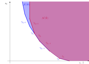
Figure 5. Comparison between ${\mathcal{N}}(\Phi)$ and ${\mathcal{N}}(\tilde{\Phi})$

Now, for any $c\in I,$ let us introduce the new variable $\tilde{z}:=z_{1}-cs_{2}^{a_{l_{1}}},$ and accordingly define

$$\tilde{\Phi}(\tilde{z},s_{2}):=\Phi(\tilde{z}+cs_{2}^{a_{l_{1}}},s_{2}).$$

Note that $\tilde{\Phi}$ is still analytic in $\tilde{z},$ but may be only fractionally analytic in $s_{2}.$ The region $D_{l_{1}}^{c}$ then corresponds to

$$\tilde{D}_{l_{1}}^{c}:=\{(\tilde{z},s_{2}):|\tilde{z}|<{\varepsilon}s_{2}^{a_{l_{1}}}\}.$$

In Step 2 of our resolution algorithm, which will be discussed in the next section, we shall base our analysis on the Newton polyhedron of $\tilde{\Phi}$ in place of ${\mathcal{N}}(\Phi).$ The corresponding vertices and compact edges of ${\mathcal{N}}(\tilde{\Phi})$ will be denoted by $(\tilde{B}_{l},\tilde{A}_{l}),l=0,\dots,\tilde{L}$ and $\tilde{\gamma}_{l}:=(\tilde{B}_{l},\tilde{A}_{l}),(\tilde{B}_{l-1},\tilde{A}_{l-1})],l=1,\dots,\tilde{L}.$ The line supporting the edge $\tilde{\gamma}_{l}$ will be denoted by $\tilde{L}_{l},$ the associated weight by $\tilde{\kappa}^{l},$ and the corresponding modulus of slope by $\tilde{a}_{l}=\tilde{\kappa}_{1}^{l}/\tilde{\kappa}_{2}^{l}.$ The corresponding homogeneous domains and transition domains into which we shall decompose the upper half-plane where $\tilde{z}\in{\mathbb{R}},s_{2}>0,$ will be denoted by $\tilde{D}_{l},l=1,\dots,\tilde{L},$ and $\tilde{E}_{l},l=0,\dots,\tilde{L}.$

Coming back to $\tilde{D}_{l_{1}}^{c},$ note that by (6.9),

(7.25) $$\tilde{\Phi}(\tilde{z},s_{2})=\tilde{U}_{0}(\tilde{z},s_{2})(\tilde{z}+cs_{2}^{a_{l_{1}}})^{\nu_{1}}\prod_{l=1}^{L}\Phi\left[\begin{matrix}\cdot\\ l\end{matrix}\right](\tilde{z}+cs_{2}^{a_{l_{1}}},s_{2}),$$

where

$$\Phi\left[\begin{matrix}\cdot\\ l\end{matrix}\right](\tilde{z}+cs_{2}^{a_{l_{1}}},s_{2})=\prod_{r\in\left[\begin{matrix}\cdot\\ l\end{matrix}\right]}(\tilde{z}+cs_{2}^{a_{l_{1}}}-r(s_{2}))=\prod_{r\in\left[\begin{matrix}\cdot\\ l\end{matrix}\right]}(\tilde{z}-\tilde{r}(s_{2})),$$

if we define adjusted roots $\tilde{r}$ by

$$\tilde{r}(s_{2}):=r(s_{2})-cs_{2}^{a_{l_{1}}}.$$

If now $l<l_{1}$ and $r\in\left[\begin{matrix}\cdot\\ l\end{matrix}\right],$ then $a_{l}<a_{l_{1}},$ so the roots $\tilde{r}(s_{2})$ and $r(s_{2})$ do have the same leading term and the same multiplicity.

Thus the identities (6.10) and (6.11) show that we indeed have

$$(\tilde{B}_{l},\tilde{A}_{l})=(B_{l},A_{l}),\quad 0\leq l<l_{1}.$$

In particular,

$$\tilde{\gamma}_{l}={\gamma}_{l}\quad\text{and}\quad\tilde{a}_{l}=a_{l},\ l<l_{1}$$

(compare Figure 5).

Case 1: $c\notin\mathcal{C}_{l_{1}}.$ Then, if $l=l_{1}$ and $r\in\left[\begin{matrix}\cdot\\ l\end{matrix}\right],$ we can factor

$$\tilde{z}-\tilde{r}(s_{2})=s_{2}^{a_{l_{1}}}\Big{(}c-c_{l_{1}}^{{\alpha}_{1}}+\frac{\tilde{z}}{s_{2}^{a_{l_{1}}}}\Big{)}+\text{higher degree terms},$$

where $|{\tilde{z}}/{s_{2}^{a_{l_{1}}}}|<{\varepsilon}.$ Moreover, if $c_{l_{1}}^{{\alpha}_{1}}$ is real, then $|c-c_{l_{1}}^{{\alpha}_{1}}|\gg{\varepsilon},$ and otherwise $|c-c_{l_{1}}^{{\alpha}_{1}}|\geq|\text{\rm Im\,}c_{l_{1}}^{{\alpha}_{1}}|>0,$ so that, by choosing ${\varepsilon}$ small enough, we can assume that in both cases $|c-c_{l_{1}}^{{\alpha}_{1}}|\gg{\varepsilon}.$ Thus we may assume that $|c-c_{l_{1}}^{{\alpha}_{1}}+{\tilde{z}}/{s_{2}^{a_{l_{1}}}}|\sim 1.$

Arguing in a similar way also for $l\neq l_{1}$ (compare our discussion in Subsection 7.2), we find that the edge $\tilde{\gamma}_{l_{1}}$ has the same slope and right endpoint as ${\gamma}_{l_{1}},$ but as left endpoint a point of the form $(0,\tilde{A}_{l_{1}}),$ and that we can factor

$$\tilde{\Phi}(\tilde{z},s_{2})=V(\tilde{z},s_{2})\,s_{2}^{\tilde{A}_{l_{1}}},\qquad(\tilde{z},s_{2})\in\tilde{D}_{l_{1}}^{c},$$

where the function $V(\tilde{z},s_{2})$ behaves in a similar way is in Subsection 7.2. In particular, here $\tilde{L}=l_{1}.$

Remark 7.5.

This shows that, by changing from $z_{1}$ to $\tilde{z},$ we can regard the region $\tilde{D}_{l_{1}}^{c}$ now like a transition domain $\tilde{E}_{\tilde{L}},$ in the coordinates $(\tilde{z},s_{2}).$ With view to Lemma 7.4, we also remark that here $\tilde{A}_{l_{1}}\geq A_{l_{1}}\geq A_{1}=1.$ These kind of domains will be handled in Step 2 of our resolution algorithm.

Case 2: $c\in\mathcal{C}_{l_{1}}.$ Then $c$ is of the form $c=c_{l_{1}}^{{\alpha}_{1}}\in{\mathbb{R}}.$ This will fix ${\alpha}_{1}$ in the sequel. We then recall from (6.12) that, up to a constant factor, the ${\kappa}^{l_{1}}$-principal part of $\Phi$ is given by

$$\Phi_{{\kappa}^{l_{1}}}(z_{1},s_{2})=s_{2}^{A_{l_{1}-1}}z_{1}^{B_{l_{1}}}\prod_{\alpha}\Big{(}z_{1}-c^{\alpha}_{l_{1}}s_{2}^{a_{l_{1}}}\Big{)}^{N\left[\begin{matrix}{\alpha}\\ l_{1}\end{matrix}\right]}.$$

Consequently, the ${\kappa}^{l_{1}}$-principal part of $\tilde{\Phi}$ is given by

$$\tilde{\Phi}_{{\kappa}^{l_{1}}}(\tilde{z},s_{2})=s_{2}^{A_{l_{1}-1}}(\tilde{z}+cs_{2}^{a_{l_{1}}})^{B_{l_{1}}}\prod_{\alpha}\Big{(}\tilde{z}-(c^{\alpha}_{l_{1}}-c_{l_{1}}^{{\alpha}_{1}})\ s_{2}^{a_{l_{1}}}\Big{)}^{N\left[\begin{matrix}{\alpha}\\ l_{1}\end{matrix}\right]}.$$

We must therefore distinguish two sub-cases:

Subcase (i): $B_{l_{1}}>0,$ or $\left[\begin{matrix}\cdot\\ l_{1}\end{matrix}\right]\supsetneqq\left[\begin{matrix}{\alpha}_{1}\\ l_{1}\end{matrix}\right].$ Then $\tilde{\Phi}_{{\kappa}^{l_{1}}}$ is not a monomial, and thus the edge $\tilde{\gamma}_{l_{1}}$ lies on the same line as ${\gamma}_{l_{1}}.$ It thus will have the same slope $\tilde{a}_{l_{1}}=a_{l_{1}}$ and right endpoint $(B_{l_{1}-1},A_{l_{1}-1})$ as ${\gamma}_{l_{1}},$ but the left endpoints of these two edges may be different.

Here

$$\tilde{E}_{l_{1}}=\{(\tilde{z},s_{2}):2^{M}s_{2}^{\tilde{a}_{l_{1}+1}}<|\tilde{z}|<2^{-M}s_{2}^{a_{l_{1}}}\}.$$

Thus, if we choose ${\varepsilon}<2^{-M},$ and decompose

$$\tilde{D}_{l_{1}}^{c}=\tilde{D}_{l_{1},1}^{c}\cup\tilde{D}_{l_{1},2}^{c},$$

where

$$\tilde{D}_{l_{1},1}^{c} := \{(\tilde{z},s_{2}):2^{M}s_{2}^{\tilde{a}_{l_{1}+1}}\leq|\tilde{z}|<{\varepsilon}s_{2}^{a_{l_{1}}}\},$$

$$\tilde{D}_{l_{1},2}^{c} := \{(\tilde{z},s_{2}):|\tilde{z}|<2^{M}s_{2}^{a_{l_{1}+1}}\},$$

then $\tilde{D}_{l_{1},1}^{c}\subset\tilde{E}_{l_{1}}.$ Note that for $l_{1}=\tilde{L},$ we even have $\tilde{D}_{l_{1}}^{c}\subset\tilde{E}_{l_{1}}.$

Moreover, clearly $\tilde{D}_{l_{1},2}^{c}$ is contained in the union of the $\tilde{E}_{l}$s and $\tilde{D}_{l}$s with $l\geq l_{1}+1,$ and therefore

$$\tilde{D}_{l_{1}}^{c}\subset\bigcup\limits_{l=l_{1}}^{\tilde{L}}\tilde{E}_{l}\,\cup\bigcup\limits_{l=l_{1}+1}^{\tilde{L}}\tilde{D}_{l}.$$

Remarks 7.6.

(a) We thus see that in Subcase (i) the contribution by $D_{l_{1}}^{c}$ to our maximal operator can be covered by the contributions by the $\tilde{E}_{l}$s with $l\geq l_{1}$ and the $\tilde{D}_{l}$s with $l\geq l_{1}+1.$ Those by the $\tilde{E}_{l}$s will be completely covered by Step 2 of our resolution algorithm in the next section, and to the $\tilde{D}_{l}$s we shall apply a similar kind of reasoning as in the present section, which will lead to Step 3 of our resolution algorithm, and so forth. Note also that $l_{1}+1\geq 2,$ so that the first edge with right endpoint $(n-2,0)$ will be the same for all steps $\geq 2,$ namely $\tilde{\gamma}_{1}.$ Thus, if $\tilde{A}_{1}\geq 1,$ then we can apply Lemma 7.4 in Step 2, and as well in any higher step.

(b) Note also that if $\tilde{a}_{l}$ with $l\geq l_{1}+1$ is the leading exponent of a root $\tilde{r}(s_{2})$ of $\tilde{\Phi},$ then $\tilde{a}_{l}$ is of the form $a_{l_{1}l_{2}}^{{\alpha}_{1}},$ and the leading term of $\tilde{r}(s_{2})$ is of the form $c_{l_{1}l_{2}}^{{\alpha}_{1}{\alpha}_{2}}s_{2}^{a_{l_{1}l_{2}}^{{\alpha}_{1}}}.$

Subcase (ii): $B_{l_{1}}=0$ and $\left[\begin{matrix}\cdot\\ l_{1}\end{matrix}\right]=\left[\begin{matrix}{\alpha}_{1}\\ l_{1}\end{matrix}\right],$ i.e., all roots in $\left[\begin{matrix}\cdot\\ l_{1}\end{matrix}\right]$ have the same leading term $cs_{2}^{a_{l_{1}}}.$ Then $\tilde{\Phi}_{{\kappa}^{l_{1}}}(\tilde{z},s_{2})=s_{2}^{A_{l_{1}-1}}\tilde{z}^{N\left[\begin{matrix}\cdot\\ l_{1}\end{matrix}\right]}=s_{2}^{A_{l_{1}-1}}\tilde{z}^{B_{l_{1}-1}}$ is a monomial, so that the edge $\tilde{\gamma}_{l_{1}}$ has “shrunk” to the vertex $(B_{l_{1}-1},A_{l_{1}-1})$ of ${\mathcal{N}}(\tilde{\Phi})$ by the change of coordinates from $z_{1}$ to $\tilde{z}.$ Here, the edge $\tilde{\gamma}_{l_{1}}$ will thus have a slope $\tilde{a}_{l_{1}}>a_{l_{1}}.$

Here

$$\tilde{E}_{l_{1}-1}=\{(\tilde{z},s_{2}):2^{M}s_{2}^{\tilde{a}_{l_{1}}}<|\tilde{z}|<2^{-M}s_{2}^{a_{l_{1}-1}}\},$$

since $\tilde{a}_{l_{1}-1}=a_{l_{1}-1}.$ And, we claim that we may assume that

$$2^{M}s_{2}^{\tilde{a}_{l_{1}}}<{\varepsilon}s_{2}^{a_{l_{1}}}\leq 2^{-M}s_{2}^{a_{l_{1}-1}}.$$

Indeed, the first inequality is equivalent to $s_{2}^{\tilde{a}_{l_{1}}-a_{l_{1}}}<{\varepsilon}2^{-M}.$ But, $\tilde{a}_{l_{1}}-a_{l_{1}}>0,$ so that the latter inequality can be assumed to be true because we may assume that $s_{2}\ll 1$ is sufficiently small. The second inequality follows in a similar way. Let us here decompose $\tilde{D}_{l_{1}}^{c}=\tilde{D}_{l_{1},1}^{c}\cup\tilde{D}_{l_{1},2}^{c},$ where now

$$\tilde{D}_{l_{1},1}^{c} := \{(\tilde{z},s_{2}):2^{M}s_{2}^{\tilde{a}_{l_{1}}}\leq|\tilde{z}|<{\varepsilon}s_{2}^{a_{l_{1}}}\},$$

$$\tilde{D}_{l_{1},2}^{c} := \{(\tilde{z},s_{2}):|\tilde{z}|<2^{M}s_{2}^{\tilde{a}_{l_{1}}}\}.$$

Then $\tilde{D}_{l_{1},1}^{c}\subset\tilde{E}_{l_{1}-1},$ in a similar way as in the previous subcase we see that here

(7.26) $$\tilde{D}_{l_{1}}^{c}\subset\bigcup\limits_{l=l_{1}-1}^{\tilde{L}}\tilde{E}_{l}\,\cup\bigcup\limits_{l=l_{1}}^{\tilde{L}}\tilde{D}_{l}.$$

Remarks 7.7.

(a) If $l_{1}=1,$ then for our phase $\Phi$ in (6.8), by (6.2) we have

(7.27) $$\begin{split}{\kappa}^{1}&=\big{(}\frac{1}{n-2},\frac{n-m}{n-2}\big{)},\quad a_{1}=\frac{1}{n-m},\\ \Phi_{{\kappa}^{1}}(z_{1},s_{2})&=z_{1}^{n-2}n(n-1)\beta(0)+s_{2}z_{1}^{m-2}m(m-1)\omega(0).\end{split}$$

Note that here $B_{l_{1}}=m-2.$ Moreover, since we are assuming that $n\geq 2m,$ we have $n-m\geq m\geq 2,$ so that the polynomial $z_{1}^{n-m}n(n-1)\beta(0)+s_{2}m(m-1)\omega(0)$ has at least 2 different (real or complex) roots, each of multiplicity 1, hence $\left[\begin{matrix}\cdot\\ 1\end{matrix}\right]\supsetneqq\left[\begin{matrix}{\alpha}_{1}\\ 1\end{matrix}\right].$ This shows that here only Subcase (i) can arise.

In particular, in Step 2, Subcase (ii) can only arise when $l_{1}\geq 2,$ and the same applies then to all higher steps, so that $l_{1}-1\geq 1$ in (7.26) – thus no transition domains $\tilde{E}_{0}$ will appear in (7.26).

(b) By (7.26) we see that in Subcase (ii) the contribution by $D_{l_{1}}^{c}$ to our maximal operator can be covered by the contributions by the $\tilde{E}_{l}$s with $l\geq l_{1}-1\geq 1$ and the $\tilde{D}_{l}$s with $l\geq l_{1}\geq 2.$ Those by the $\tilde{E}_{l}$s will be completely covered by Step 2 of our resolution algorithm in the next section, and to the $\tilde{D}_{l}$s we shall apply a similar kind of reasoning as in the present section, which will lead to Step 3 of our resolution algorithm, and so forth. Note again that since here $l_{1}\geq 2,$ the first edge with right endpoint $(n-2,0)$ will be the same for all steps $\geq 2,$ namely $\tilde{\gamma}_{1}.$ Thus, if $\tilde{A}_{1}\geq 1,$ then we can apply Lemma 7.4 in Step 2, and as well in any higher step.

(c) Note also that if $\tilde{a}_{l}$ with $l\geq l_{1}$ is the leading exponent of a root $\tilde{r}(s_{2})$ of $\tilde{\Phi},$ then $\tilde{a}_{l}$ is of the form $a_{l_{1}l_{2}}^{{\alpha}_{1}},$ and the leading term of $\tilde{r}(s_{2})$ is of the form $c_{l_{1}l_{2}}^{{\alpha}_{1}{\alpha}_{2}}s_{2}^{a_{l_{1}l_{2}}^{{\alpha}_{1}}}.$

We finally remark that, by compactness of the interval $I,$ we can cover the homogeneous domain $D_{l_{1}}$ by the sub-domains $D_{l_{1}}^{c},c\in\mathcal{C}_{l_{1}},$ and a finite number of subdomains $D_{l_{1}}^{c^{j}},$ with $c^{j}\notin\mathcal{C}_{l_{1}}.$

Thus we may reduce our studies to considering such sub-domains $D_{l_{1}}^{c},$ for which we shall then, as explained before, pass to the coordinate $\tilde{z}$ in place of $z_{1}.$ The study of the contributions of the corresponding homogeneous domains $\tilde{D}_{l_{1}}^{c}$ will be carried out in Step 2 (and higher) of our algorithm.

7.9. Stopping domains $D^{c}_{l_{1}},c\in\mathcal{C}_{l_{1}},$ for the resolution algorithm at Step 1

We shall stop on the domain $D^{c}_{l_{1}},c=c_{l_{1}}^{{\alpha}_{1}}\in\mathcal{C}_{l_{1}},$ when the multiplicity $N\left[\begin{matrix}{\alpha}_{1}\\ l_{1}\end{matrix}\right]$ of the cluster $\left[\begin{matrix}{\alpha}_{1}\\ l_{1}\end{matrix}\right]$ agrees with the multiplicity of every sub-cluster of it.

Observe that this is equivalent to the condition that the cluster $\left[\begin{matrix}{\alpha}_{1}\\ l_{1}\end{matrix}\right]$ contains only one, real root $r$ of multiplicity $N\left[\begin{matrix}{\alpha}_{1}\\ l_{1}\end{matrix}\right].$ The fact that this root must be real stems from the observation that with any root in $\left[\begin{matrix}{\alpha}_{1}\\ l_{1}\end{matrix}\right]$, its complex conjugate must also be in the same cluster, since $\Phi$ is real.

The contribution by such a domain $D^{c}_{l_{1}}$ will be covered in a complete way in Subsection 8.8 of the next section.

Remark 7.8 (Stopping when $l_{1}=1$).

If $l_{1}=1,$ we have seen in Remark 7.7 (a) that any real root in $\left[\begin{matrix}{\alpha}_{1}\\ 1\end{matrix}\right]$ has multiplicity $1,$ so that by (6.12) we do have $N\left[\begin{matrix}{\alpha}_{1}\\ 1\end{matrix}\right]=1.$ This shows that for $l_{1}=1$ we stop our resolution algorithm in Step 1.

8. Analysis in Step 2 of the resolution algorithm

In this section, we shall proceed in a similar way as in the previous Section 7, but our analysis will now be based on the coordinates $\tilde{z}$ and the function $\tilde{\Phi}$ in place of $z_{1}$ and the function $\Phi.$ Adapting the notation from the previous subsection, recall that

$$z_{1}=\tilde{z}+w(s_{2}),$$

where here $w(s_{2})=cs_{2}^{a_{l_{1}}}.$ The non-trivial extra term $w(s_{2}),$ however, will create additional challenges compared to the analysis in the previous section.

Of course, we shall have to apply the same change of coordinates also to our original phase functions $\breve{\phi}_{1}(x_{1},s_{2})$ and $\Phi_{0}(x_{1},s^{\prime}):=\breve{\phi}_{1}(x_{1},s_{2})+s_{1}x_{1}$ in (6.7), and therefore put

$$\tilde{\Phi}_{0,0}(\tilde{z},s_{2}) := \breve{\phi}_{1}(\tilde{z}+w(s_{2}),s_{2}),$$

$$\tilde{\Phi}_{0}(\tilde{z},s^{\prime}) := \Phi_{0}(\tilde{z}+w(s_{2}),s_{2})=\tilde{\Phi}_{0,0}(\tilde{z},s_{2})+s_{1}\tilde{z}+s_{1}w(s_{2}).$$

Note that then

(8.1) $$\tilde{\Phi}(\tilde{z},s_{2}):={\partial}_{\tilde{z}}^{2}\tilde{\Phi}_{0}(\tilde{z},s^{\prime})={\partial}_{\tilde{z}}^{2}\tilde{\Phi}_{0,0}(\tilde{z},s_{2})$$

(compare with (6.8)).

A crucial tool will again be Lemma 7.4. Its application will here require that $\tilde{A}_{1}\geq 1,$ so let us begin by discussing this condition.

8.1. On the condition $\tilde{A}_{1}\geq 1$

By Remark 7.5, we see that $\tilde{A}_{1}\geq 1$ in Case 1, i.e., when $c\notin\mathcal{C}_{l_{1}}.$ Assume next that we are in Case 2 where $c=c_{l_{1}}^{{\alpha}_{1}}\in\mathcal{C}_{l_{1}}.$ Then, if $l_{1}\geq 2,$ we have that $\tilde{A}_{1}=A_{1}\geq 1.$

But, in Remark 7.8 we have seen that for $l_{1}=1$ we can stop our resolution algorithm already at Step 1, so that henceforth we may and shall assume that $l_{1}\geq 2,$ hence $\tilde{A}_{1}=A_{1}\geq 1.$

For the sake of completeness, let us finally observe that when $l_{1}=1,$ then by Remark 7.7 (a) we must be in Subcase (i), and by (7.27) we have

$$\Phi_{{\kappa}^{1}}(z_{1},s_{2})=C_{1}z_{1}^{m-2}\big{(}z_{1}^{n-m}+C_{2}s_{2}\big{)}=C_{1}z_{1}^{m-2}\prod_{\alpha}\Big{(}z_{1}-c^{\alpha}_{l_{1}}s_{2}^{a_{1}}\Big{)},$$

with nontrivial real constants $C_{1},C_{2}.$ This implies that

$$\tilde{\Phi}_{{\kappa}^{1}}(\tilde{z},s_{2})=C_{1}\tilde{z}\,(\tilde{z}+c_{l_{1}}^{{\alpha}_{1}}s_{2}^{a_{1}})^{m-2}\prod_{{\alpha}\neq{\alpha}_{1}}\Big{(}\tilde{z}-(c^{\alpha}_{l_{1}}-c_{l_{1}}^{{\alpha}_{1}})\ s_{2}^{a_{1}}\Big{)},$$

where the product over the ${\alpha}$s such that ${\alpha}\neq{\alpha}_{1}$ will consist of $n-m-1\geq 1$ different factors, since all non-trivial roots of $\Phi_{{\kappa}^{1}}$ have multiplicity 1. By (6.10) this implies that $\tilde{A}_{1}=(n-3)a_{1}=(n-3)/(n-m),$ and $\tilde{B}_{1}=1,$ so that $\tilde{\gamma}_{1}=[(1,(n-3)/(n-m)),(n-2,0)].$

Thus, $\tilde{A}_{1}<1$ if and only if $m=2.$

Remarks 8.1.

(a) Notice that by Remark 7.8 and our discussion in Subsection 8.8 we see that we shall have dealt in a complete way with the contribution by the homogeneous domain $D_{1}$ and therefore will be allowed to assume that $l_{1}\geq 2$ in Step 3 and higher.

(b) We shall see later (see Section 9) that our resolution algorithm will stop whenever we have arrived at a narrow subdomain containing only one sub-cluster of roots consisting of just one root (possibly with multiplicity) whose leading jet $w(s_{2})$ is real, i.e., when no further “fine splitting” of roots can occur. In such a case we shall be able to argue in a very similar way as we are doing here.

Recall also that since the edges $\tilde{\gamma}_{1}$ and ${\gamma}_{1}$ are lying on the same line $L_{1},$ we have $\tilde{a}_{1}=a_{1},$ and

(8.2) $$\frac{\tilde{A}_{1}-1}{\tilde{a}_{1}}+\tilde{B}_{1}+2=m.$$

For later use, note that this identity remains valid even when $\tilde{A}_{1}<1.$ And, if $m\geq 3,$ so that $\tilde{A}_{1}\geq 1,$ then by Lemma 7.4 we also have

(8.3) $$\frac{\tilde{A}_{l}-1}{\tilde{a}_{l}}+\tilde{B}_{l}+2\leq m,\quad l=1,\dots,\tilde{L}.$$

Clearly, this holds true also for $l_{1}\geq 2.$

8.2. Domain decomposition and dyadic localization in $\tilde{z}$ and $s_{2}$

After having fixed $l_{1}\in\{1,\dots,L\},$ according to our discussion in the previous section we can cover the domain $\tilde{D}_{l_{1}}^{c}$ by $\tilde{\kappa}^{l}$- homogeneous domains $\tilde{D}_{l}$ of the form

$$\tilde{D}_{l}:=\{(\tilde{z},s_{2}):2^{-M}s_{2}^{\tilde{a}_{l}}\leq|\tilde{z}|\leq 2^{M}s_{2}^{\tilde{a}_{l}}\},\quad l\leq\tilde{L},$$

and transition domains of the form

$$\tilde{E}_{l} := \{(\tilde{z},s_{2}):2^{M}s_{2}^{\tilde{a}_{l+1}}<|\tilde{z}|<2^{-M}s_{2}^{\tilde{a}_{l}}\},\quad l\leq\tilde{L}-1,$$

$$\tilde{E}_{\tilde{L}} := \{(\tilde{z},s_{2}):|\tilde{z}|<2^{-M}s_{2}^{\tilde{a}_{\tilde{L}}}\}.$$

More precisely, in Case 1 where $c\notin\mathcal{C}_{l_{1}},$ according to Remark 7.5 we just need the transition domain $\tilde{E}_{\tilde{L}},$ where $\tilde{L}=l_{1}.$

In Case 2, where $c\in\mathcal{C}_{l_{1}},$ we need to distinguish two subcases: if we are in Subcase (i), then according to Remark 7.6 (a) we shall need the transition domains $\tilde{E}_{l}$ with $l\geq l_{1}\geq 1$ and the homogeneous domains $\tilde{D}_{l}$ with $l\geq l_{1}+1\geq 2.$ Moreover, according to Remark 8.1 (a), we shall treat the case $l_{1}=1$ separately (in Subsection 8.8), so that we shall here even assume that $l_{1}\geq 2.$

In Subcase (ii) of Case 2, according to Remark 7.7 we may assume that $l_{1}\geq 2$ and shall then need the transition domains $\tilde{E}_{l}$ with $l\geq l_{1}-1\geq 1$ and the homogeneous domains $\tilde{D}_{l}$ with $l\geq l_{1}\geq 2.$

Moreover, our discussion in Subsection 8.1 shows that under these assumptions we always have that $\tilde{A}_{1}\geq 1.$

Recall also that in all cases that had appeared we had seen that the edges $\tilde{\gamma}_{1}$ and ${\gamma}_{1}$ were supported on the same line $\tilde{L}_{1}=L_{1}$ of “slope” $\tilde{a}_{1}=a_{1},$ so that the identity (8.2) and the inequalities (8.3) will hold true.

Having fixed $l_{1}$ and $l$ according to these assumptions, we shall put

$$a:=a_{l_{1}},\quad\tilde{a}:=\tilde{a}_{l}.$$

Note that if we are in Case 1, or Subcase (i) of Case 2, then $\tilde{a}\geq\tilde{a}_{l_{1}}=a,$ but in Subcase (ii) it may also happen that $\tilde{a}<a$ (for instance if $l=l_{1}-1,$ where $\tilde{a}=a_{l_{1}-1}<a_{l_{1}}=a$).

Note also that, in analogy to (8.3), by Lemma 7.4 we also have

(8.4) $$\frac{\tilde{A}_{l}-1}{\tilde{a}_{l}}+\tilde{B}_{l}+2\leq m,\quad l=1,\dots,\tilde{L},$$

since $\tilde{A}_{1}\geq 1.$

As in Section 7, we shall again localize to these domains $\tilde{D}_{l}$ and $\tilde{E}_{l}$ in a smooth way by means of the corresponding functions $\tilde{\rho}_{l}$ respectively $\tilde{\tau}_{l}$ given by

$$\tilde{\rho}_{l}(\tilde{z},s_{2}):=\chi_{0}\Big{(}\frac{\tilde{z}}{2^{M}s_{2}^{\tilde{a}_{l}}}\Big{)}-\chi_{0}\Big{(}\frac{\tilde{z}}{2^{-M}s_{2}^{\tilde{a}_{l}}}\Big{)},$$

respectively

$$\tilde{\tau}_{l}(\tilde{z},s_{2}):=\chi_{0}\Big{(}\frac{\tilde{z}}{2^{-M}s_{2}^{\tilde{a}_{l}}}\Big{)}\,-\chi_{0}\Big{(}\frac{\tilde{z}}{2^{M}s_{2}^{\tilde{a}_{l+1}}}\Big{)}.$$

The corresponding functions such as $\mu^{\lambda},J({\lambda},s)$ and $F({\lambda},s_{2},s_{3},y_{1}),$ will be designated by means of an extra upper index $\tilde{\rho}_{l}$ respectively $\tilde{\tau}_{l},$ such as $\mu^{\tilde{\rho}_{l},{\lambda}},J^{\tilde{\rho}}({\lambda},s),$ or $F^{\tilde{\tau}_{l}}({\lambda},s_{2},s_{3},y_{1}).$

Similarly as before, let us here localize to

$$|\tilde{z}|\sim 2^{-j},\ s_{2}\sim 2^{-k},$$

where we may assume that $j,k$ are sufficiently large integers $\gg 1.$ To this end, we define scaled coordinates $z,{\sigma}_{2}$ by writing $\tilde{z}=2^{-j}z,\ s_{2}=2^{-k}{\sigma}_{2},$ so that

$$|z|\sim 1,\ \sigma_{2}\sim 1.$$

Accordingly, let us here put

$$\tilde{J}_{j,k}({\lambda},s) := \chi_{1}(2^{k}s_{2})\int e^{-i{\lambda}s_{3}\tilde{\Phi}_{0}(\tilde{z},s^{\prime})}\chi_{1}(2^{j}\tilde{z})\,\eta d\tilde{z}$$

$$= \chi_{1}({\sigma}_{2})\,2^{-j}\int e^{-i{\lambda}s_{3}\tilde{\Phi}_{0}^{s}(z,s_{1},{\sigma}_{2})}\chi_{1}(z)\,\eta dz,$$

where we have put

$$\tilde{\Phi}_{0}^{s}(z,s_{1},{\sigma}_{2}):=\tilde{\Phi}_{0}(2^{-j}z,s_{1},2^{-k}{\sigma}_{2}),$$

and

$$\tilde{F}_{j,k}({\lambda},2^{-k}{\sigma}_{2},s_{3},y_{1}) := 2^{-j}\iint e^{-i{\lambda}s_{3}(\tilde{\Phi}_{0}^{s}(z,s_{1},{\sigma}_{2})-s_{1}y_{1})}\chi_{0}(s_{1})\chi_{1}(z)\,\eta dzds_{1}.$$

The corresponding contribution to $\mu^{\lambda}$ is here given by

(8.5) $$\mu_{j,k}^{\lambda}(y+{\Gamma}) := {\lambda}^{\frac{5}{2}}2^{-k}\times$$

$$\iint\tilde{F}_{j,k}({\lambda},2^{-k}{\sigma}_{2},s_{3},y_{1})e^{-i{\lambda}s_{3}(s_{2}^{2}B(s_{2})-2^{-k}{\sigma}_{2}y_{2}-y_{3})}\chi_{1}({\sigma}_{2})d{\sigma}_{2}\chi_{1}(s_{3})ds_{3}.$$

Of course, we are following here the same conventions as in Subsection 7.1. Applying the same reasoning as in that subsection, in analogy to (7.1), (7.2) and (7.3) we see here that for the contribution by the transition domain $\tilde{E}_{l},$ i.e., for $J^{\tilde{\tau}_{l}},$ we may assume that $J^{\tilde{\tau}_{l}}_{j,k}\equiv 0,$ unless

(8.6) $$j\geq k\tilde{a}_{l}+M/2,\qquad\text{if}\quad l=1,\dots\tilde{L}.$$

Similarly, for the contribution by the homogeneous domain $\tilde{D}_{l},2\leq l\leq\tilde{L},$ i.e., for $J^{\tilde{\rho}_{l}},$ we may assume that $J^{\tilde{\rho}_{l}}_{j,k}\equiv 0,$ unless

(8.7) $$|j-k\tilde{a}_{l}|\leq M/2.$$

For the range of $j$s and $k$s described by (8.6), respectively (8.7), we are then also allowed to assume for simplicity that

$$J^{\tilde{\tau}_{l}}_{j,k}({\lambda},s) = J^{\tilde{\rho}_{l}}_{j,k}({\lambda},s)=\tilde{J}_{j,k}({\lambda},s).$$

The corresponding maximal operators will be designated by means of an extra lower index $j,k,$ such as ${\mathcal{M}}_{j,k}^{\lambda},$ or ${\mathcal{M}}^{\rho_{l}}_{j,k}.$

8.3. Resolution of singularity on the transition domain $\tilde{E}_{l}$

Fix $\tilde{E}_{l}$ with $l\geq l_{1},$ respectively $l\geq l_{1}-1\geq 1$ if we are in the Subcase (ii) of Case 2. Arguing as in Subsection 7.2, we may write

(8.8) $$\tilde{\Phi}(\tilde{z},s_{2})=\tilde{V}(\tilde{z},s_{2})\,s_{2}^{\tilde{A}_{l}}\tilde{z}^{\tilde{B}_{l}},\qquad(\tilde{z},s_{2})\in\tilde{E}_{l},$$

where $\tilde{V}$ is analytic in $\tilde{z}$ and fractional analytic in $s_{2}$ away from the coordinate axes and $|\tilde{V}|\sim 1.$ Moreover, by means of Lemma 7.1 we see again that there is a function $\tilde{U}(\tilde{z},s_{2})$ having similar properties as $\tilde{V}(\tilde{z},s_{2})$ such that

$${\partial}_{\tilde{z}}^{2}\big{(}\tilde{U}(\tilde{z},s_{2})s_{2}^{\tilde{A}_{l}}\tilde{z}^{\tilde{B}_{l}+2}\big{)}=\tilde{\Phi}(\tilde{z},s_{2})={\partial}_{\tilde{z}}^{2}\tilde{\Phi}_{0,0}(\tilde{z},s_{2}).$$

In particular, $|\tilde{U}|\sim 1.$ Again the function $\tilde{U}(\tilde{z},s_{2})s_{2}^{\tilde{A}_{l}}\tilde{z}^{\tilde{B}_{l}+2}$ is analytic in $\tilde{z}$ and vanishes of second order at $\tilde{z}=0.$ Consequently, we see that (compare also (8.1))

$$\tilde{\Phi}_{0,0}(\tilde{z},s_{2})=\tilde{U}(\tilde{z},s_{2})s_{2}^{\tilde{A}_{l}}\tilde{z}^{\tilde{B}_{l}+2}+\tilde{z}\tilde{g}(s_{2})+\tilde{h}(s_{2}),$$

with fractional analytic functions $\tilde{g}(s_{2}),\tilde{h}(s_{2}).$ Since $\tilde{z}=0$ iff $z_{1}=w(s_{2})$ (recall that $\tilde{z}=z_{1}-w(s_{2})$), these are explicitly given by

(8.9) $$\begin{split}\tilde{h}(s_{2})&=\breve{\phi}_{1}(w(s_{2}),s_{2}),\\ \tilde{g}(s_{2})&={\partial}_{z_{1}}\breve{\phi}_{1}(w(s_{2}),s_{2}).\end{split}$$

Consequently,

$$\tilde{\Phi}_{0}(\tilde{z},s^{\prime})=\tilde{U}(\tilde{z},s_{2})s_{2}^{\tilde{A}_{l}}\tilde{z}^{\tilde{B}_{l}+2}+s_{1}(\tilde{z}+w(s_{2}))+\tilde{z}\tilde{g}(s_{2})+\tilde{h}(s_{2}).$$

Let us finally again apply our changes of coordinates $\tilde{z}=2^{-j}z,\ s_{2}=2^{-k}{\sigma}_{2}.$ Then, if we put $A:=\tilde{A}_{l},B:=\tilde{B}_{l}$ and

$$d_{j,k}:=2^{-kA-j(B+2)},$$

assuming that (8.6) holds true, we obtain

$$\tilde{\Phi}_{0}^{s}(z,s_{1},{\sigma}_{2})-s_{1}y_{1}=d_{j,k}U^{s}(z,{\sigma}_{2}){\sigma}_{2}^{A}z^{B+2}+s_{1}(2^{-j}z+w(s_{2})-y_{1})+2^{-j}z\tilde{g}(s_{2})+\tilde{h}(s_{2}),$$

where $U$ has similar properties as in (7.7).

Remark 8.2.

Note that we have picked up in particular the new term $s_{1}w(s_{2}),$ where

$$|w(s_{2})|\sim s_{2}^{a}\sim 2^{-ka}$$

(recall that $a=a_{l_{1}}$). The same will in fact apply in all subsequent steps of our resolution algorithm, where in Step $p$ we will have to choose for $w(s_{2})$ the leading jet

$$w(s_{2}):=c_{l_{1}}^{{\alpha}_{1}}s_{2}^{a_{l_{1}}}+c_{l_{1}l_{2}}^{{\alpha}_{1}{\alpha}_{2}}s_{2}^{a_{l_{1}l_{2}}^{{\alpha}_{1}}}+\cdots+c_{l_{1}\cdots l_{p}}^{{\alpha}_{1}\cdots{\alpha}_{p}}s_{2}^{a_{l_{1}\cdots l_{p}}^{{\alpha}_{1}\cdots{\alpha}_{p-1}}}.$$

Let us then write

$$w(s_{2})=2^{-ka}{\sigma}_{2}^{a}\tilde{w}({\sigma}_{2}),$$

so that $|\tilde{w}|\sim 1,$ whereas all derivatives of $\tilde{w}$ can be assumed to be very small. We shall use the following abbreviations:

$$Y_{1}: = 2^{ka}y_{1},$$

$$\gamma({\sigma}_{2},Y_{1}) := {\sigma}_{2}^{a}\tilde{w}({\sigma}_{2})-Y_{1},$$

$$K := 2^{j-ka}.$$

These allow us to re-write

(8.10) $$\tilde{\Phi}_{0}^{s}(z,s_{1},{\sigma}_{2})-s_{1}y_{1}$$

$$= d_{j,k}U^{s}(z,{\sigma}_{2}){\sigma}_{2}^{A}z^{B+2}+2^{-j}s_{1}\big{(}K{\gamma}({\sigma}_{2},Y_{1})+z\big{)}+2^{-j}z\tilde{g}(s_{2})+\tilde{h}(s_{2}),$$

where $z\sim 1\sim{\sigma}_{2}.$ We can then re-write

$$\tilde{F}_{j,k}({\lambda},2^{-k}{\sigma}_{2},s_{3},y_{1})=2^{-j}\iint e^{-i{\lambda}s_{3}(\tilde{\Phi}_{0}^{s}(z,s_{1},{\sigma}_{2})-s_{1}y_{1})}\chi_{0}(s_{1})\chi_{1}(z)\,\eta dzds_{1}$$

(8.11) $$=2^{-j}e^{-i{\lambda}s_{3}\tilde{h}(s_{2})}\,\int{\varphi}\big{(}s_{3}{\lambda}2^{-j}[K{\gamma}({\sigma}_{2},Y_{1})+z]\big{)}$$

$$\hskip 142.26378pt\times e^{-i{\lambda}s_{3}\big{(}d_{j,k}U^{s}(z,{\sigma}_{2}){\sigma}_{2}^{A}z^{B+2}+2^{-j}z\tilde{g}(2^{-k}{\sigma}_{2})\big{)}}\chi_{1}(z)\eta dz,$$

where ${\varphi}:=\widehat{\chi_{0}}\in{\mathcal{S}}({\mathbb{R}})$ is rapidly decaying.

8.4. $L^{2}$ - estimation of ${\mathcal{M}}_{j,k}^{\lambda}$ for the contribution by $\tilde{E}_{l}$

In the same way as we had argued in Subsection 8.4, we obtain the same kind of $L^{2}$-estimate:

(8.12) $$\|{\mathcal{M}}^{\lambda}_{j,k}\|_{2\to 2}\lesssim 2^{-j}(1+{\lambda}d_{j,k})^{-\frac{1}{2}}.$$

8.5. $L^{1+{\varepsilon}}$ - estimates of ${\mathcal{M}}_{j,k}^{\lambda}$ for the contribution by $\tilde{E}_{l}$ when ${\lambda}\geq 2^{j}$

8.5.1. Reduction to $K|\gamma({\sigma}_{2},Y_{1})|\lesssim 1$

a) Let us first consider the ${\sigma}_{2}$ -region where

(8.13) $$K|\gamma({\sigma}_{2},Y_{1})|\gg 1.$$

Then $K{\gamma}({\sigma}_{2},Y_{1})+z\sim K{\gamma}({\sigma}_{2},Y_{1}).$

Case 1: ${\lambda}d_{j,k}\geq 1$. Note that this implies that

$${\lambda}\geq 2^{kA+j(B+2)}\geq 2^{2j},\quad\text{hence}\quad 2^{j}\leq{\lambda}^{\frac{1}{2}}.$$

Given any $0<{\delta}\ll 1,$ we may then assume that $K|\gamma({\sigma}_{2},Y_{1})|\geq{\lambda}^{{\delta}-1}2^{j}.$ For, if

$$1\ll K|\gamma({\sigma}_{2},Y_{1})|<{\lambda}^{{\delta}-1}2^{j},$$

then we would have $1\ll{\lambda}^{{\delta}-1/2},$ contradicting our assumption that ${\lambda}\gg 1,$ if we choose ${\delta}<1/2.$

But, if $K|\gamma({\sigma}_{2},Y_{1})|\geq\max\{1,{\lambda}^{{\delta}-1}2^{j}\},$ then $|{\lambda}2^{-j}[K{\gamma}({\sigma}_{2},Y_{1})+z]|\geq{\lambda}^{{\delta}},$ so that by (8.11) and (8.5) we see that the contribution to $\mu_{j,k}$ by this ${\sigma}_{2}$-region is a small error term of order $O({\lambda}^{-N})$ for every $N\in{\mathbb{N}}.$

Case 2: ${\lambda}d_{j,k}<1$. Here, we may ignore the term $d_{j,k}U^{s}(z,{\sigma}_{2}){\sigma}_{2}^{A}z^{B+2}$ of the phase in (8.11), since we can include the factor $e^{-i{\lambda}s_{3}(d_{j,k}U^{s}(z,{\sigma}_{2}){\sigma}_{2}^{A}z^{B+2})}$ in the amplitude. Let us thus assume that

$$\tilde{F}_{j,k}({\lambda},2^{-k}{\sigma}_{2},s_{3},y_{1}) = 2^{-j}e^{-i{\lambda}s_{3}\tilde{h}(s_{2})}\,\int{\varphi}\big{(}s_{3}{\lambda}2^{-j}[K{\gamma}({\sigma}_{2},Y_{1})+z]\big{)}$$

$$\hskip 85.35826pt\times e^{-i{\lambda}s_{3}\big{(}2^{-j}z\tilde{g}^{s}({\sigma}_{2})+\tilde{h}^{s}({\sigma}_{2})\big{)}}\chi_{1}(z)\eta dz,$$

where we have put

$$\tilde{g}^{s}({\sigma}_{2}):=\tilde{g}(2^{-k}{\sigma}_{2}),\quad\tilde{h}^{s}({\sigma}_{2}):=\tilde{h}(2^{-k}{\sigma}_{2}).$$

This case will require a more careful analysis. Observe first that by (8.9) and (6.2), we have

$$\tilde{h}(s_{2}) = w(s_{2})^{n}\beta(w(s_{2}))+s_{2}w(s_{2})^{m}\omega(w(s_{2}))+s_{2}^{2}w(s_{2})q(w(s_{2}),s_{2}),$$

$$\tilde{g}(s_{2}) = w(s_{2})^{n-1}\tilde{\beta}(w(s_{2}))+s_{2}w(s_{2})^{m-1}\tilde{\omega}(w(s_{2}))+s_{2}^{2}\tilde{q}(s_{2})=:\tilde{g}_{0}(s_{2})+s_{2}^{2}\tilde{q}(s_{2}).$$

Note that the term $s_{2}^{2}w(s_{2})q(w(s_{2}),s_{2})$ can be absorbed by the term $s_{2}^{2}B(s_{2})$ in (8.5), by slightly modifying the definition of $B(s_{2}),$ still keeping the condition $|B(s_{2})|\sim 1.$ Let us therefore henceforth simply assume that

$$\tilde{h}(s_{2})=w(s_{2})^{n}\beta(w(s_{2}))+s_{2}w(s_{2})^{m}\omega(w(s_{2})).$$

Lemma 8.3.

For every ${\alpha}\in{\mathbb{N}},$ the following estimate holds true:

$$|{\partial}_{{\sigma}_{2}}^{\alpha}\tilde{h}^{s}({\sigma}_{2})|\lesssim 2^{-k(1+ma)},\qquad|{\partial}_{{\sigma}_{2}}^{\alpha}\tilde{g}_{0}^{s}({\sigma}_{2})|\lesssim 2^{-k(1+(m-1)a)},\quad\text{if}\quad{\sigma}_{2}\sim 1.$$

Proof.

Note that

$$na-(1+ma)=(n-m)a-1\geq(n-m)a_{1}-1=0,$$

so that $na\geq 1+ma$ and also $(n-1)a\geq 1+(m-1)a.$ Since $|w(s_{2})|\sim s_{2}^{a}\sim 2^{-ka},$ the claimed estimates now follow easily. Q.E.D.

Subcase 2.a: ${\lambda}2^{-ka}\lesssim 1.$ Here, by Lemma 8.3, ${\lambda}\tilde{h}^{s}({\sigma}_{2})=O(2^{-k})$ and ${\lambda}\tilde{g}_{0}^{s}({\sigma}_{2})=O(2^{-k}),$ since $m\geq 2.$ We may thus ignore the terms $\tilde{h}^{s}({\sigma}_{2})$ and $2^{-j}z\tilde{g}_{0}({\sigma}_{2})$ in the amplitude of $\tilde{F}_{j,k}.$

Moreover, since we shall here not use any oscillation from the $z$-integration, we may also assume that the term $2^{-j}zs_{2}^{2}\tilde{q}(s_{2})$ stemming from our decomposition of $\tilde{g}(s_{2})$ is absorbed by the term $s_{2}^{2}B(s_{2})$ in (8.5), so that

$$\tilde{F}_{j,k}({\lambda},2^{-k}{\sigma}_{2},s_{3},y_{1})=2^{-j}\iint e^{-i{\lambda}s_{3}2^{-j}s_{1}[K{\gamma}({\sigma}_{2},Y_{1})+z]}\chi_{0}(s_{1})\chi_{1}(z)\,\eta dzds_{1}.$$

Note also that

$${\lambda}2^{-j}[K{\gamma}({\sigma}_{2},Y_{1})+z]={\lambda}2^{-ka}{\sigma}_{2}^{a}\tilde{w}({\sigma}_{2})-{\lambda}2^{-ka}Y_{1}+{\lambda}2^{-j}z.$$

The first term ${\lambda}2^{-ka}{\sigma}_{2}^{a}\tilde{w}({\sigma}_{2})$ can later on be included into the amplitude in (8.5), since ${\lambda}2^{-ka}\lesssim 1,$ so that we can ignore this term.

Assume first that $|Y_{1}|\gg 1.$ Then $1\ll|K{\gamma}({\sigma}_{2},Y_{1})|\sim K|Y_{1}|,$ hence

(8.14) $${\lambda}2^{-j}|K{\gamma}({\sigma}_{2},Y_{1})+z|\sim{\lambda}2^{-ka}|Y_{1}|.$$

We can then proceed in a similar way as we did in the first part of Subsection 7.4.

If $|Y_{1}|\gg 1$ and $|Y_{1}|\geq{\lambda}^{{\delta}-1}2^{ka},$ integrations by parts in $s_{1}$ show that $F_{j,k}=O({\lambda}^{-N})$ for every $N\in{\mathbb{N}},$ and thus also $\mu_{j,k}^{\lambda}(y+{\Gamma})=O({\lambda}^{-N})$ for every $N\in{\mathbb{N}},$ which shows that this leads just to a small error term.

So, assume next that

$$1\ll|Y_{1}|\lesssim{\lambda}^{{\delta}-1}2^{ka}.$$

We then decompose this region into the regions

$$\Delta_{\iota_{1}}:=\{y:|Y_{1}|\sim 2^{\iota_{1}}\},$$

where clearly we may assume that $1\ll\iota_{1}\lesssim k.$ We further decompose $\Delta_{\iota_{1}}$ into the subregions

$$\Delta_{\iota_{1},\iota_{2}} := \{y:|Y_{1}|\sim 2^{\iota_{1}},|Y_{2}|\sim 2^{\iota_{2}}\},\quad 1\ll\iota_{2}\leq k,$$

$$\Delta_{\iota_{1},0} := \{y:|Y_{1}|\sim 2^{\iota_{1}},|Y_{2}|\lesssim 1\}.$$

Then

$$|\Delta_{\iota_{1},\iota_{2}}|\lesssim 2^{\iota_{1}+\iota_{2}-ka-k}.$$

For $y\in\Delta_{\iota_{1}},$ then we may integrate by parts in $s_{1}.$ Moreover, if $\iota_{2}\gg 1,$ and if ${\lambda}2^{-2k+\iota_{2}}\geq 1,$ then our preceding discussion and (7.11) show that we can also integrate by parts in ${\sigma}_{2},$ and altogether this leads to the following estimate for $\mu_{k,j,\iota}^{\lambda}:$

$$|\mu_{j,k,\iota}^{\lambda}(y+{\Gamma})|\lesssim{\lambda}^{\frac{5}{2}}2^{-j-k}({\lambda}2^{-ka}2^{\iota_{1}})^{-1}({\lambda}2^{-2k}2^{\iota_{2}})^{-1}={\lambda}^{\frac{1}{2}}2^{-j+k+ka-\iota_{1}-\iota_{2}}.$$

Thus, Lemma 5.4 shows that, for every ${\varepsilon}>0,$

$$\|{\mathcal{M}}_{j,k,\iota}^{\lambda}\|_{1+{\varepsilon}\to 1+{\varepsilon}}\lesssim{\lambda}^{\frac{1}{2}}2^{-j}.$$

And, if $\iota_{2}=0,$ we can again apply van der Corput’s estimate of order 2 in ${\sigma}_{2},$ which leads to

$$|\mu_{j,k,\iota}^{\lambda}(y+{\Gamma})|\lesssim{\lambda}^{\frac{5}{2}}2^{-j-k}({\lambda}2^{-ka}2^{\iota_{1}})^{-1}({\lambda}2^{-2k})^{-\frac{1}{2}}={\lambda}2^{-j+ka-\iota_{1}},$$

hence

$$\|{\mathcal{M}}_{j,k,(\iota_{1},0)}^{\lambda}\|_{1+{\varepsilon}\to 1+{\varepsilon}}\lesssim{\lambda}^{1+{\varepsilon}}2^{-j-k}.$$

These estimate have to be summed over the $\iota_{2}$s, which will produce an extra factor of order $O(k).$ However, later on we have to sum over the $j$s and $k$s such that $k\lesssim j/\tilde{a},$ so effectively by summing we shall only pick up a factor of order $O(2^{{\varepsilon}j}),$ where we may choose ${\varepsilon}>0$ as small as we need; this will cause no harm.

Assume next that $|Y_{1}|\lesssim 1.$ Here we decompose into the regions

$$\Delta_{\iota_{2}} := \{y:|Y_{1}|\lesssim 1,|Y_{2}|\sim 2^{\iota_{2}}\},\quad 1\ll\iota_{2}\leq k,$$

$$\Delta_{0} := \{y:|Y_{1}|,|Y_{2}|\lesssim 1\}.$$

Then

$$|\Delta_{\iota_{2}}|\lesssim 2^{\iota_{2}-ka-k}.$$

We can now only gain from integration by parts (respectively an application of van der Corput’s estimate) in ${\sigma}_{2},$ and thus obtain

$$|\mu_{j,k,\iota_{2}}^{\lambda}(y+{\Gamma})|\lesssim{\lambda}^{\frac{5}{2}}2^{-j-k}({\lambda}2^{-2k}2^{\iota_{2}})^{-1}={\lambda}^{\frac{3}{2}}2^{-j+k-\iota_{2}}\lesssim{\lambda}^{\frac{1}{2}}2^{-j+k+ka-\iota_{2}},$$

where we have used our assumption ${\lambda}2^{-ka}\lesssim 1.$ Similarly,

$$|\mu_{j,k,0}^{\lambda}(y+{\Gamma})|\lesssim{\lambda}^{\frac{5}{2}}2^{-j-k}({\lambda}2^{-2k})^{-\frac{1}{2}}={\lambda}^{2}2^{-j}\lesssim{\lambda}2^{-j+ka}.$$

This shows that we arrive at the same estimates as before, if we choose $\iota_{1}=0$ therein.

Subcase 2.b: ${\lambda}2^{-ka}\gg 1.$ Assume again first that $|Y_{1}|\gg 1,$ so that (8.14) holds true.

If $|Y_{1}|\geq{\lambda}^{\delta}$ for some ${\delta}$ such that $0<{\delta}\ll 1,$ then ${\lambda}2^{-j}|K{\gamma}({\sigma}_{2},Y_{1})+z|\gtrsim{\lambda}^{{\delta}},$ hence

(8.15) $$\mu_{j,k}^{\lambda}(y+\Gamma)=O({\lambda}^{-N})\qquad\text{for every}\quad N\in{\mathbb{N}},$$

since ${\varphi}$ is rapidly decaying, so this case contributes again only a small error term.

So, assume next w.l.o.g. that $1\ll|Y_{1}|\leq{\lambda}^{\delta}.$ Then

(8.16) $$|y_{1}|\lesssim{\lambda}^{\delta}2^{-ka},$$

and, by (8.14),

(8.17) $$|{\varphi}\big{(}s_{3}{\lambda}2^{-j}[K{\gamma}({\sigma}_{2},Y_{1})+z]\big{)}|\lesssim({\lambda}2^{-ka}|Y_{1}|)^{-N}\leq({\lambda}2^{-ka})^{-N}$$

for every $N\in{\mathbb{N}}.$

Again, if ${\lambda}2^{-ka}\geq{\lambda}^{\delta},$ this implies (8.15), so let us assume that ${\lambda}2^{-ka}\leq{\lambda}^{\delta}.$ Then, by Lemma 8.3, since $m\geq 2,$

$$|{\lambda}\tilde{h}^{s}({\sigma}_{2})|\lesssim{\lambda}2^{-k(1+ma)}={\lambda}^{1-m}({\lambda}2^{-ka})^{m}2^{-k}\ll{\lambda}^{1-m}{\lambda}^{{\delta}m}\leq{\lambda}^{{\delta}m-1}\ll 1,$$

if we choose ${\delta}>0$ sufficiently small. Similarly,

$$|{\lambda}2^{-j}z\tilde{g}_{0}^{s}({\sigma}_{2})|\lesssim 2^{-j}{\lambda}2^{-k(1+(m-1)a)}\leq 2^{-j}({\lambda}2^{-ka})2^{-k}.$$

Let us next write $\tilde{a}=da,$ where $d>0.$ Since we are on $\tilde{E}_{l},$ by (8.6) we then have that $j\geq k\tilde{a}=kda.$ Thus, for every ${\varepsilon}>0,$

$$|{\lambda}2^{-j}z\tilde{g}_{0}^{s}({\sigma}_{2})| \lesssim 2^{-kda}({\lambda}2^{-ka})2^{-k}={\lambda}^{-{\varepsilon}}({\lambda}2^{-ka})^{1+{\varepsilon}}2^{-k(1+da-a{\varepsilon})}$$

$$\leq {\lambda}^{-{\varepsilon}+{\delta}(1+{\varepsilon})}2^{-k(1+da-a{\varepsilon})}.$$

Choosing first ${\varepsilon}>0$ sufficiently small, and then ${\delta}>0$ sufficiently small, we see that also $|{\lambda}2^{-j}z\tilde{g}_{0}^{s}({\sigma}_{2})|\ll 1.$

We may thus again ignore the terms $\tilde{h}^{s}({\sigma}_{2})$ and $2^{-j}z\tilde{g}_{0}({\sigma}_{2})$ in the amplitude of $\tilde{F}_{j,k},$ so that we may assume that

(8.18) $$\mu_{j,k}^{\lambda}(y+{\Gamma}) = {\lambda}^{\frac{5}{2}}2^{-j-k}\iint{\varphi}\big{(}s_{3}{\lambda}2^{-j}[K{\gamma}({\sigma}_{2},Y_{1})+z]\big{)}\,e^{i{\lambda}s_{3}y_{3}}(1-\chi_{0}(K{\gamma}({\sigma}_{2},Y_{1})))$$

$$\hskip 5.69046pt\times e^{-i{\lambda}s_{3}2^{-2k}\Big{(}{\sigma}_{2}^{2}\big{(}B(2^{-k}{\sigma}_{2})+2^{-j}z\tilde{q}^{s}({\sigma}_{2})\big{)}-{\sigma}_{2}Y_{2}\Big{)}}\chi_{1}(z)\chi_{1}({\sigma}_{2})\chi_{1}(s_{3})\eta dzd{\sigma}_{2}ds_{3}.$$

Here, we assume that $\chi_{0}\equiv 1$ on a sufficiently large neighborhood of the origin, and we have put $Y_{2}:=2^{k}y_{2}.$

Reduction to $|Y_{2}|\lesssim 1.$ Note that here

$$\Big{|}{\partial}_{{\sigma}_{2}}\big{(}{\varphi}\big{(}s_{3}{\lambda}2^{-j}[K{\gamma}({\sigma}_{2},Y_{1})+z]\big{)}\big{)}\Big{|} \lesssim {\lambda}2^{-ka}\Big{|}{\varphi}^{\prime}\big{(}s_{3}{\lambda}2^{-j}[K{\gamma}({\sigma}_{2},Y_{1})+z]\big{)}\Big{|}$$

$$\lesssim \Big{|}\tilde{\varphi}\big{(}s_{3}{\lambda}2^{-j}[K{\gamma}({\sigma}_{2},Y_{1})+z]\big{)}\Big{|},$$

where $\tilde{\varphi}\in{\mathcal{S}}({\mathbb{R}})$, and where we have used (8.14) and $1\leq|Y_{1}|$ for the last inequality. Note that also the ${\sigma}_{2}$-derivative of $\chi_{0}(K{\gamma}({\sigma}_{2},Y_{1}))$ can be controlled in a similar way, since $K=2^{j}2^{-ka}\leq{\lambda}2^{-ka}.$

Thus, the ${\sigma}_{2}$-derivative of the amplitude in (8.18) behaves in the same way as the factor itself. In a similar way as in Subsection 7.4, let us consider now the subregions

$$\Delta_{\iota} := \{y:1\ll|Y_{1}|\leq{\lambda}^{\delta},|Y_{2}|\sim 2^{\iota}\},\quad 1\ll\iota_{2}\leq k.$$

Since for $y\in\Delta_{\iota}$

$$\Big{|}{\partial}_{{\sigma}_{2}}\Big{(}{\sigma}_{2}^{2}\big{(}B(2^{-k}{\sigma}_{2})+2^{-j}z\tilde{q}^{s}({\sigma}_{2})\big{)}-{\sigma}_{2}Y_{2}\Big{)}\Big{|}\sim 2^{\iota},$$

an integration by parts in ${\sigma}_{2},$ using also (8.17) with $N=1,$ shows that

$$|\mu_{j,k}^{\lambda}(y+{\Gamma})|={\lambda}^{\frac{5}{2}}2^{-j-k}({\lambda}2^{-ka})^{-1}\,({\lambda}2^{-2k}2^{\iota})^{-1}={\lambda}^{\frac{1}{2}}2^{-j}2^{k(a+1)}2^{-\iota}.$$

And, by (8.16), we find that $|\Delta_{\iota}|\lesssim{\lambda}^{\delta}2^{-ka}2^{-k}2^{\iota},$ so that we conclude that

$$\|{\mathcal{M}}_{j,k,\iota}^{\lambda}\|_{1+{\varepsilon}\to 1+{\varepsilon}}\lesssim{\lambda}^{\frac{1}{2}+{\varepsilon}}2^{-j},$$

provided we choose ${\delta}>0$ sufficiently small. Here, ${\mathcal{M}}_{j,k,\iota}^{\lambda}$ denotes the contribution by $\Delta_{\iota}$ to ${\mathcal{M}}_{j,k}^{\lambda}.$ Thus, we obtain the following analogue of (7.12):

$$\sum\limits_{1\ll\iota\leq k}\|{\mathcal{M}}_{j,k,\iota}^{\lambda}\|_{1+{\varepsilon}\to 1+{\varepsilon}}\lesssim{\lambda}^{\frac{1}{2}+{\varepsilon}}2^{-j}.$$

We have thus reduced ourselves to the region

$$\Delta_{0}:=\{y:1\ll|Y_{1}|\leq{\lambda}^{\delta},|Y_{2}|\lesssim 1\}.$$

Here, we apply van der Corput’s estimate of order $2$ (Lemma 5.1) in ${\sigma}_{2}$ and obtain

$$|\mu_{j,k}^{\lambda}(y+{\Gamma})|={\lambda}^{\frac{5}{2}}2^{-j-k}({\lambda}2^{-ka})^{-1}\,({\lambda}2^{-2k})^{-\frac{1}{2}}={\lambda}2^{-j}2^{ka},$$

whereas $|\Delta_{0}|\lesssim{\lambda}^{\delta}2^{-ka}2^{-k},$ so that we shall here obtain the estimate

$$\|{\mathcal{M}}_{j,k,0}^{\lambda}\|_{1+{\varepsilon}\to 1+{\varepsilon}}\lesssim{\lambda}^{1+{\varepsilon}}2^{-j-k}$$

as in (7.13) of Section 7, and altogether we arrive also here at the estimate (7.14) for the contribution by the region where $|Y_{1}|\gg 1.$

We have thus reduced ourselves to estimating the contribution by the region where $|Y_{1}|\lesssim 1.$ Recall also that we are still assuming (8.13) and ${\lambda}2^{-j}\geq 1.$

We next observe that we can further reduce to the case where $1\ll|K{\gamma}({\sigma}_{2},Y_{1})|\lesssim 2^{j}{\lambda}^{{\delta}-1},$ again with $0<{\delta}\ll 1,$ for if $|K{\gamma}({\sigma}_{2},Y_{1})|\gg 2^{j}{\lambda}^{{\delta}-1},$ we see from (8.18) that the contribution to $\mu_{j,k}$ by this ${\sigma}_{2}$-region is a small error term of order $O({\lambda}^{-N})$ for every $N\in{\mathbb{N}}.$

So, let us assume that

$${\sigma}_{2}\in\Sigma:=\{{\sigma}_{2}\sim 1:|{\gamma}({\sigma}_{2},Y_{1})|\lesssim{\lambda}^{{\delta}-1}2^{ka}\}.$$

Then $|\Sigma|\lesssim{\lambda}^{{\delta}-1}2^{ka},$ and thus

$$\iint\limits_{\Sigma}\big{|}{\varphi}\big{(}s_{3}{\lambda}2^{-j}[K{\gamma}({\sigma}_{2},Y_{1})+z]\big{)}\big{|}\,\chi_{1}({\sigma}_{2})|\eta|dzd{\sigma}_{2}\lesssim|\Sigma|({\lambda}2^{-j})^{-1}={\lambda}^{{\delta}-2}2^{j+ka},$$

hence, by (8.18),

$$|\mu_{j,k}^{\lambda}(y+{\Gamma})|={\lambda}^{\frac{5}{2}}2^{-j-k}{\lambda}^{{\delta}-2}2^{j+ka}={\lambda}^{\frac{1}{2}+{\delta}}2^{k(a-1)}.$$

Moreover, since here $y\in\Delta:=\{y:1\ll|Y_{1}|\lesssim 1\},$ where $|\Delta|\lesssim 2^{-ka},$ by choosing ${\delta}>0$ sufficiently small we may conclude that

$$\|{\mathcal{M}}_{j,k,|Y_{1}|\lesssim 1}^{\lambda}\|_{1+{\varepsilon}\to 1+{\varepsilon}}\lesssim{\lambda}^{\frac{1}{2}+{\varepsilon}}2^{-k}.$$

Note that this type of estimate had not yet appeared in Section 7.

b) We have thus reduced ourselves to estimating the contribution by the ${\sigma}_{2}$ -region where

(8.19) $$K|\gamma({\sigma}_{2},Y_{1})|\lesssim 1.$$

A look at the phase $\tilde{\Phi}_{0}^{s}(z,s_{1},{\sigma}_{2})-s_{1}y_{1}$ in (8.10) then shows that we can now again apply Lemma 5.2 in the variables $(s_{1},z)$ in place of $(\eta,x)$ to the oscillatory integral $\tilde{F}_{j,k}({\lambda},2^{-k}{\sigma}_{2},s_{3},y_{1})$ in (8.11), with $N:={\lambda}2^{-j}\geq 1.$ Moreover, observe that $s_{1}$ and $z$ result from our original coordinates $s_{1}$ and $z_{1}=x_{1}$ by means of a smooth change of coordinates. Passing back to our original coordinate, according to Remarks 5.3 we therefore must evaluate the original phase $\breve{\phi}_{1}(x_{1},s_{2})+s_{1}x_{1}-s_{1}y_{1}$ in (6.6) at $x_{1}=y_{1},$ and thus get

$$\tilde{F}_{j,k}({\lambda},2^{-k}{\sigma}_{2},s_{3},y_{1})=({\lambda}2^{-j})^{-1}2^{-j}e^{-i{\lambda}s_{3}(\breve{\phi}_{1}(y_{1},s_{2})}\eta(y_{1},2^{-k}{\sigma}_{2}).$$

This implies that

$$\mu_{j,k,K|{\gamma}|\lesssim 1}^{\lambda}(y+{\Gamma}) = {\lambda}^{\frac{3}{2}}2^{-k}\int e^{-i{\lambda}s_{3}\big{(}\breve{\phi}_{1}(y_{1},2^{-k}{\sigma}_{2})+2^{-2k}{\sigma}_{2}^{2}B(2^{-k}{\sigma}_{2})-2^{-k}{\sigma}_{2}y_{2}-y_{3}\big{)}}$$

$$\hskip 56.9055pt\times\chi_{1}({\sigma}_{2})\chi_{1}(s_{3})\,\chi_{0}(K{\gamma}({\sigma}_{2},Y_{1}))\,\eta d{\sigma}_{2}ds_{3}$$

for the contribution by the region where $K|{\gamma}({\sigma}_{2},Y_{1})|\lesssim 1.$ By (6.2), we have

$$\breve{\phi}_{1}(y_{1},2^{-k}{\sigma}_{2}):=y_{1}^{n}\beta(y_{1})+2^{-k}{\sigma}_{2}y_{1}^{m}\omega(y_{1})+2^{-2k}{\sigma}_{2}^{2}y_{1}q(y_{1},2^{-k}{\sigma}_{2}).$$

The last term can be absorbed by the term $2^{-2k}{\sigma}_{2}^{2}B(2^{-k}{\sigma}_{2}),$ by slightly modifying $B(s_{2})$ to $B(s_{2},y_{1}),$ which allows us to assume for simplicity that $q\equiv 0.$ Then we may re-write

$$\mu_{j,k,K|{\gamma}|\lesssim 1}^{\lambda}(y+{\Gamma}) = {\lambda}^{\frac{3}{2}}2^{-k}\int e^{-is_{3}{\lambda}\big{(}2^{-k}\Phi_{1}({\sigma}_{2},y)+y_{1}^{n}\beta(y_{1})-y_{3}\big{)}}$$

$$\hskip 56.9055pt\times\chi_{1}({\sigma}_{2})\chi_{1}(s_{3})\,\chi_{0}(K{\gamma}({\sigma}_{2},Y_{1}))\,\eta d{\sigma}_{2}ds_{3},$$

where the phase $\Phi_{1}({\sigma}_{2},y)$ is given by

$$\Phi_{1}({\sigma}_{2},y):=-{\sigma}_{2}[y_{2}-y_{1}^{m}\omega(y_{1})]+2^{-k}{\sigma}_{2}^{2}B(2^{-k}{\sigma}_{2},y_{1}).$$

We shall now distinguish two subcases:

The subcase where $K\lesssim 1.$ We claim that then our assumption (8.19) implies that $|y_{1}|\lesssim 2^{-j}.$

To this end, note first that the condition $K\lesssim 1$ is equivalent to $2^{-ka}\lesssim 2^{-j}.$ Thus, if $|Y_{1}|\lesssim 1,$ then $|y_{1}|\lesssim 2^{-ka}\lesssim 2^{-j}.$ And, if $|Y_{1}|\gg 1,$ then $1\gtrsim K|{\gamma}({\sigma}_{2},Y_{1}))|\sim K|Y_{1}|=2^{j}|y_{1}|,$ so that again $|y_{1}|\lesssim 2^{-j}.$

Observe next that here all ${\sigma}_{2}$-derivatives of $\chi_{0}(K{\gamma}({\sigma}_{2},Y_{1}))$ are uniformly bounded. This shows that we can now just follow the arguments from the last part of Subsection 7.4 (after identity (7.15)), by either integrating by parts in ${\sigma}_{2},$ or applying van der Corput’s estimates, in order to arrive again at estimates of the form (7.16) for the corresponding contributions to ${\mathcal{M}}_{j,k}^{\lambda}$ (notice that in Subsection 7.4 the quantity $Y_{1}$ had been defined in a different way, so that there $|Y_{1}|\lesssim 1$ had been equivalent to $|y_{1}|\lesssim 2^{-j}$).

The subcase where $K\gg 1.$ Here we see that necessarily $|Y_{1}|\lesssim 1.$ We shall again try to follow our reasoning from Subsection 7.4, but shall see that the case $\iota_{2}=0$ will still require a more refined reasoning.

Let us again decompose the region where $|Y_{1}|\lesssim 1$ into the subregions

$$\Delta_{\iota_{2}} := \{y:|Y_{1}|\lesssim 1,2^{k}|y_{2}-y_{1}^{m}\omega(y_{1})|\sim 2^{\iota_{2}}\},1\ll\iota_{2}\leq k,$$

$$\Delta_{0} := \{y:|Y_{1}|\lesssim 1,2^{k}|y_{2}-y_{1}^{m}\omega(y_{1})|\lesssim 1\}.$$

Then

$$|\Delta_{\iota_{2}}|\lesssim 2^{-ka}2^{\iota_{2}-k}.$$

Assume first that $\iota_{2}\gg 1.$ Observe first that

$$\int\Big{|}{\partial}_{{\sigma}_{2}}\big{(}\chi_{0}(K{\gamma}({\sigma}_{2},Y_{1}))\chi_{1}({\sigma}_{2})\eta\big{)}\Big{|}\,d{\sigma}_{2}\lesssim K\int\big{|}\chi^{\prime}_{0}(K{\gamma}({\sigma}_{2},Y_{1}))\big{|}\chi_{1}({\sigma}_{2})\,d{\sigma}_{2}\lesssim 1,$$

since here ${\sigma}_{2}\sim 1,$ so that we may use $\tau_{2}:={\sigma}_{2}^{a}\tilde{w}({\sigma}_{2})$ as a new variable of integration in place of ${\sigma}_{2}.$ Thus, we may again integrate by parts in ${\sigma}_{2}$ and obtain that

$$|\mu_{j,k,K|{\gamma}|\lesssim 1,\iota_{2}}^{\lambda}(y+{\Gamma})|\lesssim{\lambda}^{\frac{3}{2}}2^{-k}({\lambda}2^{-2k+\iota_{2}})^{-1}={\lambda}^{\frac{1}{2}}2^{k-\iota_{2}},$$

hence

(8.20) $$\|{\mathcal{M}}_{j,k,K|{\gamma}|\lesssim 1,\iota_{2}}^{\lambda}\|_{1+{\varepsilon}\to 1+{\varepsilon}}\lesssim{\lambda}^{\frac{1}{2}+{\varepsilon}}2^{-ka}.$$

Note that this type of estimate had not yet appeared in Section 7.

Assume finally that $\iota_{2}=0.$ Then a direct application of van der Corput’s estimate of order 2 in ${\sigma}_{2}$ would lead in a similar way to the estimate

$$\|{\mathcal{M}}_{j,k,K|{\gamma}|\lesssim 1,0}^{\lambda}\|_{1+{\varepsilon}\to 1+{\varepsilon}}\lesssim{\lambda}2^{-k}2^{-ka},$$

which turns out to be insufficient. Indeed, we shall need to gain a factor $K^{-1}=2^{ka}2^{-j}$ over this estimate, which will require a more refined argument.

Note first that $|{\partial}_{{\sigma}_{2}}{\gamma}({\sigma}_{2},Y_{1})|\sim 1.$ This allows us to write, for ${\sigma}_{2}\sim 1,$

$${\gamma}({\sigma}_{2},Y_{1})=(\sigma_{2}-\sigma_{2}^{c})W(\sigma_{2},Y_{1}),$$

where ${\sigma}_{2}^{c}={\sigma}_{2}(Y_{1})$ and $W$ are analytic functions with $|{\sigma}_{2}^{c}|\sim 1\sim|W|.$ It is then natural to change coordinates from ${\sigma}_{2}$ to

$$\tau_{2}:=K({\sigma}_{2}-{\sigma}_{2}^{c}),\quad\text{i.e.,}\quad{\sigma}_{2}={\sigma}_{2}^{c}+K^{-1}\tau_{2}.$$

Then, for $y\in\Delta_{0},$ we may assume that, with respect to our new variables of integration,

(8.21) $$\mu_{j,k,K|{\gamma}|\lesssim 1,0}^{\lambda}(y+{\Gamma}) = {\lambda}^{\frac{3}{2}}2^{-k}K^{-1}\int e^{-is_{3}{\lambda}\big{(}2^{-k}\Phi_{2}(\tau_{2},y)+y_{1}^{n}\beta(y_{1})-y_{3}\big{)}}$$

$$\hskip 56.9055pt\times\chi_{1}({\sigma}_{2}^{c}+K^{-1}\tau_{2})\chi_{1}(s_{3})\,\chi_{0}(\tau_{2})\,\eta d\tau_{2}ds_{3},$$

where

$$\Phi_{2}(\tau_{2},y):=\Phi_{1}({\sigma}_{2}^{c}+K^{-1}\tau_{2},y)=-\big{(}{\sigma}_{2}[y_{2}-y_{1}^{m}\omega(y_{1})]+2^{-k}{\sigma}_{2}^{2}B(2^{-k}{\sigma}_{2},y_{1})\big{)}\Big{|}_{{\sigma}_{2}:={\sigma}_{2}^{c}+K^{-1}\tau_{2}}.$$

Since $y\in\Delta_{0},$ we may further write

$$y_{2}-y_{1}^{m}\omega(y_{1})=:2^{-k}Y_{2},\quad\text{where}\quad|Y_{2}|\lesssim 1,$$

so that

$$\Phi_{2}(\tau_{2},y)=\Phi_{1}({\sigma}_{2}^{c}+K^{-1}\tau_{2},y)=2^{-k}\big{(}-{\sigma}_{2}Y_{2}+{\sigma}_{2}^{2}B(2^{-k}{\sigma}_{2},y_{1})\big{)}\Big{|}_{{\sigma}_{2}:={\sigma}_{2}^{c}(Y_{1})+K^{-1}\tau_{2}}.$$

By performing a Taylor expansion of the phase function $\Phi_{1}({\sigma}_{2}^{c}+K^{-1}\tau_{2},y)$ with respect to $K^{-1}\tau_{2},$ we see that we may write

$${\lambda}2^{-k}\Phi_{2}(\tau_{2},y)={\lambda}2^{-2k}\Big{(}H_{0}(Y)+K^{-1}\tau_{2}\,H_{1}(Y)+K^{-2}\tau_{2}^{2}\,H_{2}(Y,K^{-1}\tau_{2})\Big{)},$$

where the $H_{j}$ are analytic functions of their very variables, and where

(8.22) $$|H_{2}|\sim 1,\qquad H_{1}(Y)=-(Y_{2}-A(y_{1}))=-2^{k}\big{(}y_{2}-y_{1}^{m}{\omega}(y_{1})-2^{-k}A(y_{1})\big{)}.$$

Here, $A(y_{1})=2{\sigma}_{2}^{c}(Y_{1})B(0,y_{1})+D(y_{1}),$ with an error term $D(y_{1})$ of order $O(2^{-k}).$ Note also that

$$\big{|}{\partial}_{\tau_{2}}^{2}\big{[}\tau_{2}^{2}H_{2}(Y,K^{-1}\tau_{2})\big{]}\big{|}\sim 1,\qquad\big{|}{\partial}_{\tau_{2}}\big{[}\tau_{2}^{2}H_{2}(Y,K^{-1}\tau_{2})\big{]}\big{|}\lesssim 1,$$

since $K\gg 1.$

We are thus led to decomposing the $y$-region $\Delta_{0}$ into the following subsets:

$$\Delta_{0,\nu} := \{y\in\Delta_{0}:|H_{1}(Y)|\sim 2^{\nu}K^{-1}\},\qquad 1\ll\nu\lesssim\log K\leq\log{\lambda};$$

$$\Delta_{0,0} := \{y\in\Delta_{0}:|H_{1}(Y)|\lesssim K^{-1}\}.$$

As usually, the corresponding measures will be denoted by $\mu_{j,k,\nu}^{\lambda},$ and so forth. Since $2^{ka}|y_{1}|=|Y_{1}|\lesssim 1$ on $\Delta_{0},$ in combination with (8.22) we see that

(8.23) $$|\Delta_{0,\nu}|\lesssim 2^{-ka}2^{-k}2^{\nu}K^{-1}.$$

Assume first that $\nu\gg 1.$ Then an integration by parts with respect to $\tau_{2}$ in (8.21) leads to

$$|\mu_{j,k,\nu}^{\lambda}(y+\Gamma)|\lesssim{\lambda}^{\frac{3}{2}}2^{-k}K^{-1}\big{[}{\lambda}2^{-2k}\,2^{\nu}K^{-2}\big{]}^{-1}={\lambda}^{\frac{1}{2}}2^{k-\nu}K,$$

hence, in combination with (8.23),

$$\|{\mathcal{M}}_{j,k,\nu}^{\lambda}\|_{1+{\varepsilon}\to 1+{\varepsilon}}\lesssim{\lambda}^{\frac{1}{2}+{\varepsilon}}2^{-ka},$$

i.e., the same type of estimate as in (8.20).

Assume next that $\nu=0.$ Here, we can again apply van der Corput’s estimate of order 2 in $\tau_{2}$ and obtain that

$$|\mu_{j,k,0}^{\lambda}(y+\Gamma)|\lesssim{\lambda}^{\frac{3}{2}}2^{-k}K^{-1}\big{[}{\lambda}2^{-2k}\,K^{-2}\big{]}^{-\frac{1}{2}}={\lambda},$$

hence

$$\|{\mathcal{M}}_{j,k,0}^{\lambda}\|_{1+{\varepsilon}\to 1+{\varepsilon}}\lesssim{\lambda}2^{-ka}2^{-k}K^{-1}={\lambda}^{1+{\varepsilon}}2^{-j-k},$$

which is again of the form (7.13).

Combining all the estimates from this subsection, we see that in analogy with the estimate (7.16) which we had established for Step 1, for Step 2 we obtain that for every ${\varepsilon}>0$ we have the following estimate:

(8.24) $$\|{\mathcal{M}}_{j,k}^{\lambda}\|_{1+{\varepsilon}\to 1+{\varepsilon}}\lesssim{\lambda}^{1+{\varepsilon}}2^{-j-k}+{\lambda}^{\frac{1}{2}+{\varepsilon}}2^{-j}+{\lambda}^{\frac{1}{2}+{\varepsilon}}2^{-k}+{\lambda}^{\frac{1}{2}+{\varepsilon}}2^{-ka}.$$

8.6. $L^{p}$ - estimates of ${\mathcal{M}}_{j,k}^{\lambda}$ for the contribution by $E_{l}$ when ${\lambda}\geq 2^{j}$

Interpolation between the $L^{2}$ - estimate (8.12) and the $L^{1+{\varepsilon}}$ - estimate (8.24) leads to

$$\|{\mathcal{M}}_{j,k}^{\lambda}\|_{p\to p} \lesssim ({\lambda}^{1+{\varepsilon}}2^{-k})^{\frac{2}{p}-1}(1+{\lambda}d_{j,k})^{-\frac{1}{2}(2-\frac{2}{p})}2^{-j}+({\lambda}^{\frac{1}{2}+{\varepsilon}})^{\frac{2}{p}-1}(1+{\lambda}d_{j,k})^{-\frac{1}{2}(2-\frac{2}{p})}2^{-j}$$

$$+ ({\lambda}^{\frac{1}{2}+{\varepsilon}}2^{-k})^{\frac{2}{p}-1}\big{(}2^{-j}(1+{\lambda}d_{j,k})^{-\frac{1}{2}}\big{)}^{2-\frac{2}{p}}$$

$$+ ({\lambda}^{\frac{1}{2}+{\varepsilon}}2^{-ka})^{\frac{2}{p}-1}\big{(}2^{-j}(1+{\lambda}d_{j,k})^{-\frac{1}{2}}\big{)}^{2-\frac{2}{p}}$$

$$\lesssim {\lambda}^{{\varepsilon}^{\prime}}({\lambda}d_{j,k})^{\frac{2}{p}-1}(1+{\lambda}d_{j,k})^{\frac{1}{p}-1}\,(d_{j,k}^{-1})^{\frac{2}{p}-1}\,2^{-k(\frac{2}{p}-1)}\,2^{-j}$$

$$+\,{\lambda}^{{\varepsilon}^{\prime}}({\lambda}d_{j,k})^{\frac{1}{p}-\frac{1}{2}}(1+{\lambda}d_{j,k})^{\frac{1}{p}-1}\,(d_{j,k}^{-1})^{\frac{1}{p}-\frac{1}{2}}2^{-j}$$

$$+{\lambda}^{{\varepsilon}^{\prime}}({\lambda}d_{j,k})^{\frac{1}{p}-\frac{1}{2}}(1+{\lambda}d_{j,k})^{\frac{1}{p}-1}\,(d_{j,k}^{-1})^{\frac{1}{p}-\frac{1}{2}}\,2^{-k(\frac{2}{p}-1)}2^{-j(2-\frac{2}{p})}$$

$$+{\lambda}^{{\varepsilon}^{\prime}}({\lambda}d_{j,k})^{\frac{1}{p}-\frac{1}{2}}(1+{\lambda}d_{j,k})^{\frac{1}{p}-1}\,(d_{j,k}^{-1})^{\frac{1}{p}-\frac{1}{2}}\,2^{-ka(\frac{2}{p}-1)}2^{-j(2-\frac{2}{p})},$$

if $1<p<2.$ Arguing as in Subsection 7.5, we see that we can sum over all dyadic ${\lambda}$s and obtain that, for every ${\varepsilon}^{\prime}>0,$

$$\sum\limits_{{\lambda}\gg 1}\|{\mathcal{M}}_{j,k}^{\lambda}\|_{p\to p} \lesssim (d_{j,k}^{-1}2^{-k})^{\frac{2}{p}-1+{\varepsilon}^{\prime}}\,2^{-j}+(d_{j,k}^{-1})^{\frac{1}{p}-\frac{1}{2}+{\varepsilon}^{\prime}}\,2^{-j}$$

$$+ (d_{j,k}^{-1})^{\frac{1}{p}-\frac{1}{2}+{\varepsilon}^{\prime}}\,2^{-k(\frac{2}{p}-1)}2^{-j(2-\frac{2}{p})}$$

$$+ (d_{j,k}^{-1})^{\frac{1}{p}-\frac{1}{2}+{\varepsilon}^{\prime}}\,2^{-ka(\frac{2}{p}-1)}2^{-j(2-\frac{2}{p})}.$$

Recall next that $A=\tilde{A}_{l},B=\tilde{B}_{l},$ so that by (8.4)

$$\frac{A-1}{\tilde{a}}+B+2\leq m,\quad\text{and}\quad d_{j,k}^{-1}=2^{kA+j(B+2)}.$$

Moreover, since we are on $\tilde{E}_{l},$ by (8.6) we have $j\geq k\tilde{a}.$ This shows that we can argue in exactly the same way as in Subsection 7.6 in order to show that we can sum the first two terms on the right-hand side of (8.6) over all $k$s and $j$s such that $j\geq k\tilde{a}.$

This leaves us with showing that

(8.26) $$\sum\limits_{j,k\gg 1:j\geq k\tilde{a}}\Big{(}(d_{j,k}^{-1})^{\frac{1}{p}-\frac{1}{2}+{\varepsilon}^{\prime}}\,2^{-k(\frac{2}{p}-1)}2^{-j(2-\frac{2}{p})}+(d_{j,k}^{-1})^{\frac{1}{p}-\frac{1}{2}+{\varepsilon}^{\prime}}\,2^{-ka(\frac{2}{p}-1)}2^{-j(2-\frac{2}{p})}\Big{)}<\infty,$$

provided ${\varepsilon}^{\prime}>0$ is sufficiently small.

But, if $j\geq k\tilde{a},$ since $A\geq 1,$ we see that

$$(d_{j,k}^{-1})^{\frac{1}{p}-\frac{1}{2}+{\varepsilon}^{\prime}}\,2^{-k(\frac{2}{p}-1)}2^{-j(2-\frac{2}{p})} = (2^{kA+j(B+2)})^{\frac{1}{p}-\frac{1}{2}+{\varepsilon}^{\prime}}\,2^{-k(\frac{2}{p}-1)}2^{-j(2-\frac{2}{p})}$$

$$= (2^{k(A-1)+j(B+2)})^{\frac{1}{p}-\frac{1}{2}+{\varepsilon}^{\prime}}\,2^{-k(\frac{1}{p}-\frac{1}{2}-{\varepsilon}^{\prime})}2^{-j(2-\frac{2}{p})}$$

$$\leq 2^{j\big{(}\frac{A-1}{\tilde{a}}+B+2\big{)}(\frac{1}{p}-\frac{1}{2}+{\varepsilon}^{\prime})}\,2^{-k(\frac{1}{p}-\frac{1}{2}-{\varepsilon}^{\prime})}2^{-j(2-\frac{2}{p})}$$

$$\leq 2^{jm(\frac{1}{p}-\frac{1}{2}+{\varepsilon}^{\prime})}\,2^{-k(\frac{1}{p}-\frac{1}{2}-{\varepsilon}^{\prime})}2^{-j(2-\frac{2}{p})}$$

$$= 2^{j\big{[}m(\frac{1}{p}-\frac{1}{2}+{\varepsilon}^{\prime})+\frac{2}{p}-2\big{]}}\,2^{-k(\frac{1}{p}-\frac{1}{2}-{\varepsilon}^{\prime})}.$$

But,

$$m(\frac{1}{p}-\frac{1}{2})+\frac{2}{p}-2<m\frac{1}{2m}+\frac{2}{p}-2=\frac{2}{p}-\frac{3}{2}<0,$$

since $p>\max\{3/2,h\}.$ Thus we see that if we choose ${\varepsilon}^{\prime}$ sufficiently small, then both the exponent of $2^{j}$ as well as that of $2^{k}$ in the last estimate are negative, so that we can sum these estimates over all $j,k\geq 1.$

We are thus left with the second sum in (8.26). But, since $j\geq k\tilde{a},$

$$(d_{j,k}^{-1})^{\frac{1}{p}-\frac{1}{2}+{\varepsilon}^{\prime}}\,2^{-ka(\frac{2}{p}-1)}2^{-j(2-\frac{2}{p})} = (2^{kA+j(B+2)})^{\frac{1}{p}-\frac{1}{2}+{\varepsilon}^{\prime}}\,2^{-ka(\frac{2}{p}-1)}2^{-j(2-\frac{2}{p})}$$

$$= (2^{k(A-1)+j(B+2)})^{\frac{1}{p}-\frac{1}{2}+{\varepsilon}^{\prime}}\,2^{k(\frac{1}{p}-\frac{1}{2}+{\varepsilon}^{\prime})-ka(\frac{2}{p}-1)}2^{-j(2-\frac{2}{p})}$$

$$\leq 2^{j\big{(}\frac{A-1}{\tilde{a}}+B+2\big{)}(\frac{1}{p}-\frac{1}{2}+{\varepsilon}^{\prime})}\,2^{k(\frac{1}{p}-\frac{1}{2}+{\varepsilon}^{\prime}-\frac{2a}{p}+a)}2^{-j(2-\frac{2}{p})}$$

$$\leq 2^{j\big{[}m(\frac{1}{p}-\frac{1}{2}+{\varepsilon}^{\prime})+\frac{2}{p}-2\big{]}}\,2^{k(\frac{1}{p}-\frac{1}{2}+{\varepsilon}^{\prime}-\frac{2a}{p}+a)}.$$

Again, we may assume that the exponent of $2^{j}$ is strictly negative.

Assume first that $\tilde{a}\geq a.$ Then $j\geq ka,$ hence after summing first in $j\geq ka,$ we are left with the sum

$$\sum\limits_{k\geq 1}2^{ka\big{[}m(\frac{1}{p}-\frac{1}{2}+{\varepsilon}^{\prime})+\frac{2}{p}-2\big{]}}\,2^{k(\frac{1}{p}-\frac{1}{2}+{\varepsilon}^{\prime}-\frac{2a}{p}+a)}.$$

But, the exponent of $2^{k}$ can be estimated as follows:

$$a\big{[}m(\frac{1}{p}-\frac{1}{2})+\frac{2}{p}-2\big{]}+\frac{1}{p}-\frac{1}{2}-\frac{2a}{p}+a = (am+1)(\frac{1}{p}-\frac{1}{2})-a$$

$$<(am+1)\frac{1}{n}-a=\frac{1-(n-m)a}{n}\leq 0,$$

since $p>h$ and $a\geq a_{1}=1/(n-m).$ By choosing ${\varepsilon}^{\prime}$ sufficiently small, we can thus finally also sum over all $k\geq 1.$

Assume finally that $\tilde{a}<a.$ Then $-2a/p+a=-2a(1/p-1/2)<-2\tilde{a}(1/p-1/2)=-2\tilde{a}/p+\tilde{a},$ so that we can here estimate

$$(d_{j,k}^{-1})^{\frac{1}{p}-\frac{1}{2}+{\varepsilon}^{\prime}}\,2^{-ka(\frac{2}{p}-1)}2^{-j(2-\frac{2}{p})} \leq 2^{j\big{[}m(\frac{1}{p}-\frac{1}{2}+{\varepsilon}^{\prime})+\frac{2}{p}-2\big{]}}\,2^{k(\frac{1}{p}-\frac{1}{2}+{\varepsilon}^{\prime}-\frac{2\tilde{a}}{p}+\tilde{a})}.$$

Thus, after summing first in $j\geq k\tilde{a},$ we are left with the sum

$$\sum\limits_{k\geq 1}2^{k\tilde{a}\big{[}m(\frac{1}{p}-\frac{1}{2}+{\varepsilon}^{\prime})+\frac{2}{p}-2\big{]}}\,2^{k(\frac{1}{p}-\frac{1}{2}+{\varepsilon}^{\prime}-\frac{2\tilde{a}}{p}+\tilde{a})}.$$

From here on, we can argue as before, only with $a$ replaced by $\tilde{a};$ note here that also $\tilde{a}\geq a_{1}.$

This concludes the proof of estimate (8.26).

8.7. $L^{p}$ - estimates of ${\mathcal{M}}_{j,k}^{\lambda}$ for the contribution by $E_{l}$ and $\tilde{E}_{l}$ when ${\lambda}<2^{j}$

We shall study here both the situations in Step 1 as well as in Step 2. Let us begin by observing that the condition ${\lambda}<2^{j}$ implies that

(8.27) $${\lambda}d_{j,k}<2^{-j}\ll 1.$$

This implies by (7.9), respectively (8.12), that here we have the $L^{2}$-estimate

(8.28) $$\|{\mathcal{M}}^{\lambda}_{j,k}\|_{2\to 2}\lesssim 2^{-j}.$$

As for the $L^{1+{\varepsilon}}$-estimates, let us first look at the Step 1-situation and the contribution by $E_{l}$: By (7.10) and (8.27), we may here assume that

$$\Phi_{0}^{s}(z,s_{1},{\sigma}_{2})-s_{1}y_{1}=-s_{1}y_{1};$$

the exponentials of all other terms of the phase can be included into the amplitude. Thus,

$$F_{j,k}({\lambda},2^{-k}{\sigma}_{2},s_{3},y_{1}) = 2^{-j}\iint e^{-i{\lambda}s_{3}(\Phi_{0}^{s}(z,s_{1},{\sigma}_{2})-s_{1}y_{1})}\chi_{0}(s_{1})\chi_{1}(z)\,\eta dzds_{1}$$

$$\sim 2^{-j}{\varphi}(-{\lambda}s_{3}y_{1}),$$

where ${\varphi}:=\widehat{\chi_{0}}\in{\mathcal{S}}({\mathbb{R}})$ is rapidly decaying. This shows that, up to a small error term, we can reduce to the region where

$$|y_{1}|\leq{\lambda}^{{\delta}-1},$$

where again we may later on choose ${\delta}>0$ as small as we like. But then we obtain

(8.29) $$\mu_{j,k}^{\lambda}(y+{\Gamma}) = {\lambda}^{\frac{5}{2}}2^{-j-k}$$

$$\times\int e^{-i{\lambda}s_{3}(2^{-2k}{\sigma}_{2}^{2}B(2^{-k}{\sigma}_{2})-2^{-k}{\sigma}_{2}y_{2}-y_{3})}\chi_{1}({\sigma}_{2})d{\sigma}_{2}\chi_{1}(s_{3})\,{\varphi}(-{\lambda}s_{3}y_{1})ds_{3}.$$

Let us first assume that ${\lambda}\geq 2^{k}.$ In a similar way as in Subsection 7.4 we may then decompose the remaining $y$-region into the subregions

$$\Delta_{\iota} := \{y:|y_{1}|\leq{\lambda}^{{\delta}-1},|y_{2}|\sim 2^{\iota-k}\},\quad 1\ll\iota\leq k,$$

$$\Delta_{0} := \{y:|y_{1}|\leq{\lambda}^{{\delta}-1},|y_{2}|\lesssim 2^{-k}\}.$$

Then

$$|\Delta_{\iota}|\lesssim{\lambda}^{{\delta}-1}2^{\iota-k}.$$

And, as before, if $\iota\gg 1,$ an integration by parts in ${\sigma}_{2}$ shows that

$$|\mu_{j,k,\iota}^{\lambda}(y+{\Gamma})|\lesssim{\lambda}^{\frac{5}{2}}2^{-j-k}({\lambda}2^{\iota-2k})^{-1}={\lambda}^{\frac{3}{2}}2^{-j}2^{k-\iota}.$$

Hence, if we choose ${\delta}$ sufficiently small,

$$\|{\mathcal{M}}_{j,k,\iota}^{\lambda}\|_{1+{\varepsilon}\to 1+{\varepsilon}}\lesssim{\lambda}^{\frac{3}{2}+{\varepsilon}/2}2^{-j}2^{k-\iota}{\lambda}^{{\delta}-1}2^{\iota-k}\lesssim{\lambda}^{\frac{1}{2}+{\varepsilon}}2^{-j},$$

which leads to the following analogue of (7.12):

$$\sum\limits_{\iota\leq k}\|{\mathcal{M}}_{j,k,\iota}^{\lambda}\|_{1+{\varepsilon}\to 1+{\varepsilon}}\lesssim{\lambda}^{\frac{1}{2}+{\varepsilon}}2^{-j}.$$

If $\iota=0,$ we can again apply van der Corput’s estimate and obtain in a similar way that $\|{\mathcal{M}}_{j,k,0}^{\lambda}\|_{1+{\varepsilon}\to 1+{\varepsilon}}\lesssim{\lambda}^{1+{\varepsilon}}2^{-j-k}.$ Altogether, we thus obtain the following analogue of (7.16):

$$\|{\mathcal{M}}_{j,k}^{\lambda}\|_{1+{\varepsilon}\to 1+{\varepsilon}}\lesssim{\lambda}^{1+{\varepsilon}}2^{-j-k}+{\lambda}^{\frac{1}{2}+{\varepsilon}}2^{-j}.$$

Interpolating the estimates (8.28) and (7.16), we find that for $1<p<2,$

$$\|{\mathcal{M}}_{j,k}^{\lambda}\|_{p\to p}\lesssim({\lambda}^{1+{\varepsilon}}2^{-k})^{\frac{2}{p}-1}2^{-j}+({\lambda}^{\frac{1}{2}+{\varepsilon}})^{\frac{2}{p}-1}2^{-j}.$$

As for the first term, summing over all $k\geq 0$ and all dyadic ${\lambda}$s such that ${\lambda}<2^{j},$ we are left with the sum

$$\sum\limits_{j\geq 0}2^{j\big{(}(1+{\varepsilon})(\frac{2}{p}-1)-1\big{)}},$$

which is easily seen to be convergent if we choose ${\varepsilon}>0$ sufficiently small.

As for the second term, summing first over all all $k\leq\log{\lambda}$ and then all dyadic ${\lambda}$s that ${\lambda}<2^{j},$ we are left with the sum

$$\sum\limits_{j\geq 0}2^{j\big{(}(\frac{1}{2}+{\varepsilon})(\frac{2}{p}-1)-1\big{)}},$$

with an ${\varepsilon}>0$ which may have to be chosen slightly bigger than before. Again, it is easily seen that the latter series is convergent if we choose ${\varepsilon}>0$ sufficiently small, since $p>3/2.$

Let us finally assume that ${\lambda}<2^{k}.$ Then the “oscillatory integral” $\mu_{j,k}^{\lambda}(y+{\Gamma})$ has indeed essentially no oscillation, so that we only get the estimates

$$|\mu_{j,k}^{\lambda}(y+{\Gamma})|\lesssim{\lambda}^{\frac{5}{2}}2^{-j-k}\quad\text{and}\quad|\Delta|\lesssim{\lambda}^{{\delta}-1},$$

where $\Delta:=\{y:|y_{1}|\leq{\lambda}^{{\delta}-1},|y_{2}|\ll 1\}.$ Thus,

$$\|{\mathcal{M}}_{j,k}^{\lambda}\|_{1+{\varepsilon}\to 1+{\varepsilon}}\lesssim{\lambda}^{\frac{3}{2}+{\varepsilon}}2^{-j-k},$$

hence

$$\|{\mathcal{M}}_{j,k}^{\lambda}\|_{p\to p}\lesssim({\lambda}^{\frac{3}{2}+{\varepsilon}}2^{-k})^{\frac{2}{p}-1}2^{-j}.$$

Summing first over all $j$s such that $2^{j}>{\lambda}$ and all $k$s such that $2^{k}>{\lambda},$ we are left with the sum

$$\sum\limits_{{\lambda}\gg 1}{\lambda}^{\big{(}(\frac{3}{2}+{\varepsilon}-1)(\frac{2}{p}-1)-1\big{)}}.$$

But, $(3/2-1)(2/p-1)-1=1/p-3/2<-5/6,$ since $p>3/2,$ so that the sum is again convergent if we choose ${\varepsilon}>0$ sufficiently small.

Let us next look at the Step 2-situation and the contribution by $\tilde{E}_{l}$: By (8.10) and (8.27), we may here assume that

$$\tilde{\Phi}_{0}^{s}(z,s_{1},{\sigma}_{2})-s_{1}y_{1}=s_{1}2^{-ka}{\gamma}({\sigma}_{2},Y_{1})+\tilde{h}(s_{2}),$$

where $z\sim 1\sim{\sigma}_{2}.$ Putting again $\tilde{h}^{s}({\sigma}_{2}):=\tilde{h}(2^{-k}{\sigma}_{2}),$ we find that

$$\tilde{F}_{j,k}({\lambda},2^{-k}{\sigma}_{2},s_{3},y_{1})=2^{-j}e^{-i{\lambda}s_{3}\tilde{h}^{s}({\sigma}_{2})}\,\int{\varphi}\big{(}s_{3}{\lambda}2^{-ka}{\gamma}({\sigma}_{2},Y_{1})\big{)}\chi_{1}(z)\eta dz,$$

where ${\varphi}:=\widehat{\chi_{0}}\in{\mathcal{S}}({\mathbb{R}})$ is rapidly decaying and, by (8.5),

$$\mu_{j,k}^{\lambda}(y+{\Gamma}) = {\lambda}^{\frac{5}{2}}2^{-k}\times$$

$$\iint\tilde{F}_{j,k}({\lambda},2^{-k}{\sigma}_{2},s_{3},y_{1})e^{-i{\lambda}s_{3}(s_{2}^{2}B(s_{2})-2^{-k}{\sigma}_{2}y_{2}-y_{3})}\chi_{1}({\sigma}_{2})d{\sigma}_{2}\chi_{1}(s_{3})ds_{3}.$$

Assume first that ${\lambda}2^{-ka}\geq 1.$ We then decompose in $y$ into the regions

$$\Delta_{\iota} := \{y:|Y_{1}|\sim 2^{\iota}\},\quad 1\ll\iota\leq ka,$$

$$\Delta_{0} := \{y:|Y_{1}|\lesssim 1\},$$

and denote the corresponding contributions by $\mu_{j,k,\iota}^{\lambda}.$ Then

$$|\Delta_{\iota}|\lesssim 2^{\iota}2^{-ka}.$$

And, if $\iota\gg 1,$ then clearly

$$|\tilde{F}_{j,k,\iota}({\lambda},2^{-k}{\sigma}_{2},s_{3},y_{1})|\lesssim 2^{-j}({\lambda}2^{-ka}2^{\iota})^{-1},$$

hence

$$|\mu_{j,k,\iota}^{\lambda}(y+{\Gamma})|\lesssim{\lambda}^{\frac{5}{2}}2^{-j-k}({\lambda}2^{-ka}2^{\iota})^{-1}.$$

This implies that

(8.30) $$\|{\mathcal{M}}_{j,k,\iota}^{\lambda}\|_{1+{\varepsilon}\to 1+{\varepsilon}}\lesssim{\lambda}^{\frac{3}{2}+{\varepsilon}}2^{-j-k}.$$

Finally, if $\iota=0,$ we can estimate

$$|\mu_{j,k,0}^{\lambda}(y+{\Gamma})|\lesssim{\lambda}^{\frac{5}{2}}2^{-j-k}\int\big{|}{\varphi}\big{(}s_{3}{\lambda}2^{-ka}{\gamma}({\sigma}_{2},Y_{1})\big{)}\big{|}\chi_{1}({\sigma}_{2})d{\sigma}_{2}\,\chi_{1}(s_{3})\chi_{1}(z)dzds_{3}.$$

But,

$$\int\big{|}{\varphi}\big{(}s_{3}{\lambda}2^{-ka}({\sigma}_{2}^{a}\tilde{w}({\sigma}_{2})-Y_{1})\big{)}\big{|}\chi_{1}({\sigma}_{2})d{\sigma}_{2}\lesssim({\lambda}2^{-ka})^{-1},$$

since ${\sigma}_{2}\sim 1,$ so that we may use $\tau_{2}:={\sigma}_{2}^{a}\tilde{w}({\sigma}_{2})$ as a new variable of integration in place of ${\sigma}_{2}.$ Thus,

$$|\mu_{j,k,0}^{\lambda}(y+{\Gamma})|\lesssim{\lambda}^{\frac{5}{2}}2^{-j-k}({\lambda}2^{-ka})^{-1},$$

so that (8.30) remains valid also for $\iota=0.$ Interpolation with (8.28) leads to

$$\|{\mathcal{M}}_{j,k,\iota}^{\lambda}\|_{p\to p}\lesssim\big{(}{\lambda}^{\frac{3}{2}+{\varepsilon}}2^{-k}\big{)}^{\frac{2}{p}-1}2^{-j}.$$

Summing the estimate in first in $\iota\leq ka,$ then in $k\geq 0$ and next over all $j$s such that $2^{j}>{\lambda},$ we are left with the sum

$$\sum\limits_{{\lambda}\gg 1}{\lambda}^{(\frac{3}{2}+{\varepsilon})(\frac{2}{p}-1)}{\lambda}^{-1}={\lambda}^{\frac{3}{p}-\frac{5}{2}+{\varepsilon}^{\prime}},$$

where ${\varepsilon}^{\prime}>0$ can be chosen as small as we like. Since $p>3/2,$ we have that $3/p-5/2<2-5/2<0,$ so that the remaining series in ${\lambda}$ is convergent.

Assume next that ${\lambda}2^{-ka}<1.$ Here, we must again invoke Lemma 8.3. According to this lemma, we have that for ${\sigma}_{2}\sim 1,$

$$|{\partial}_{{\sigma}_{2}}^{\alpha}\tilde{h}^{s}({\sigma}_{2})|\lesssim 2^{-k(1+ma)}.$$

This implies that ${\lambda}2^{-k(1+ma)}\ll{\lambda}2^{-ka}<1,$ which shows that we can now include the factor $e^{-i{\lambda}s_{3}\tilde{h}^{s}({\sigma}_{2})}$ of $\tilde{F}_{j,k}({\lambda},2^{-k}{\sigma}_{2},s_{3},y_{1})$ in the oscillatory integral defining $\mu_{j,k}^{\lambda}(y+{\Gamma})$ into the amplitude. I.e., we may simply assume that $\tilde{h}^{s}\equiv 0,$ and thus write

$$\mu_{j,k}^{\lambda}(y+{\Gamma}) = {\lambda}^{\frac{5}{2}}2^{-j-k}\times$$

$$\hskip-56.9055pt\iint e^{-i{\lambda}s_{3}(2^{-2k}{\sigma}_{2}^{2}B(2^{-k}{\sigma}_{2})-2^{-k}{\sigma}_{2}y_{2}-y_{3})}\chi_{1}({\sigma}_{2}){\varphi}\big{(}s_{3}{\lambda}2^{-ka}{\gamma}({\sigma}_{2},Y_{1})\big{)}\eta d{\sigma}_{2}\,\chi_{1}(s_{3})ds_{3}.$$

But note that ${\lambda}2^{-ka}{\gamma}({\sigma}_{2},Y_{1})={\lambda}2^{-ka}{\sigma}_{2}^{a}\tilde{w}({\sigma}_{2})-{\lambda}y_{1},$ where the first term is harmless, since ${\lambda}2^{-ka}\leq 1.$ A comparison with the identity (8.29) thus shows that we may now argue exactly as we did for the Step 1- situation.

This concludes our discussion of the case where ${\lambda}<2^{j}.$

8.8. $L^{p}$ - estimates for the contributions by domains $D_{l_{1}}^{c},c\in\mathcal{C}_{l_{1}},$ when the algorithm stops after step 1

Assume now that $c=c^{{\alpha}_{1}}_{l_{1}}\in\mathcal{C}_{l_{1}}$ is such that the cluster $\left[\begin{matrix}{\alpha}_{1}\\ l_{1}\end{matrix}\right]$ contains only one, real root $r_{0}$ of multiplicity $N_{0}:=N\left[\begin{matrix}{\alpha}_{1}\\ l_{1}\end{matrix}\right].$ The leading term of $r_{0}(s_{2})$ is then given by $c^{{\alpha}_{1}}_{l_{1}}s_{2}^{a},$ where again $a:=a_{l_{1}}.$

We can then modify our change of coordinates by re-defining

$$\tilde{z}:=z_{1}-r_{0}(s_{2}),\qquad\text{and}\qquad\tilde{\Phi}(\tilde{z},s_{2}):=\Phi(\tilde{z}+r_{0}(s_{2}),s_{2}).$$

The domain corresponding to $D_{l_{1}}^{c}$ is then essentially again of the form

$$\tilde{D}_{l_{1}}^{c}=\{(\tilde{z},s_{2}):|\tilde{z}|<{\varepsilon}s_{2}^{a_{l_{1}}}\},$$

with $0<{\varepsilon}\ll 1.$ We claim that then also on $\tilde{D}_{l_{1}}^{c}$ we have a good resolution of singularities of $\tilde{\Phi},$ namely

(8.31) $$\tilde{\Phi}(\tilde{z},s_{2})=\tilde{V}(\tilde{z},s_{2})\,s_{2}^{\tilde{A}}\tilde{z}^{N_{0}},\qquad(\tilde{z},s_{2})\in\tilde{D}_{l_{1}}^{c},$$

for some $\tilde{A}\geq 1,$ where $\tilde{V}$ has similar properties as in (8.8).

Indeed, in analogy to (7.25), we have that

$$\tilde{\Phi}(\tilde{z},s_{2})=\tilde{U}_{0}(\tilde{z},s_{2})(\tilde{z}+r_{0}(s_{2}))^{\nu_{1}}\prod_{l=1}^{L}\Phi\left[\begin{matrix}\cdot\\ l\end{matrix}\right](\tilde{z}+r_{0}(s_{2}),s_{2}).$$

Since $|\tilde{z}|\ll|r_{0}(s_{2})|,$ by modifying $\tilde{U}_{0}(\tilde{z},s_{2})$ appropriately, we may replace here $(\tilde{z}+r_{0}(s_{2}))^{\nu_{1}}$ by $s_{2}^{a\nu_{1}},$ as well as $\Phi\left[\begin{matrix}\cdot\\ l\end{matrix}\right](\tilde{z}+r_{0}(s_{2}),s_{2})$ by the following:

– if $l<l_{1},$ then by $s_{2}^{a_{l}N\left[\begin{matrix}\cdot\\ l\end{matrix}\right]};$

– if $l=l_{1},$ then by $\prod\limits_{{\alpha}\neq{\alpha}_{1}}s_{2}^{aN\left[\begin{matrix}{\alpha}\\ l_{1}\end{matrix}\right]}\,\tilde{z}^{N_{0}};$

– if $l>l_{1},$ then by $s_{2}^{aN\left[\begin{matrix}\cdot\\ l\end{matrix}\right]}.$

This shows that indeed (8.31) holds true. Moreover, a quite similar reasoning shows that the ${\kappa}^{l_{1}}$-principal part of $\tilde{\Phi}$ is given by

$$\tilde{\Phi}_{{\kappa}^{l_{1}}}={\rm constant}\,(\tilde{z}+cs_{2}^{a})^{\nu_{1}}\prod\limits_{l<l_{1}}s_{2}^{a_{l}N\left[\begin{matrix}\cdot\\ l\end{matrix}\right]}\prod\limits_{{\alpha}\neq{\alpha}_{1}}\big{(}\tilde{z}-(c_{l_{1}}^{{\alpha}}-c_{l_{1}}^{{\alpha}_{1}})s_{2}^{a}\big{)}^{N\left[\begin{matrix}{\alpha}\\ l_{1}\end{matrix}\right]}\,\tilde{z}^{N_{0}}\prod\limits_{l>l_{1}}(\tilde{z}+cs_{2}^{a})^{N\left[\begin{matrix}\cdot\\ l\end{matrix}\right]}.$$

The term with the smallest power of $\tilde{z}$ in this ${\kappa}^{l_{1}}$ - homogenous function agrees with a constant multiple of $s_{2}^{\tilde{A}}\tilde{z}^{N_{0}},$ which shows that the Newton-Puiseux polyhedron of $\tilde{\Phi}$ must be of the type sketched in Figure 6.

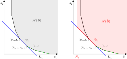
Figure 6. Stopping: comparison between ${\mathcal{N}}(\Phi)$ and ${\mathcal{N}}(\tilde{\Phi})$

Consequently, we see that $\tilde{L}=l_{1},$ $(\tilde{B}_{\tilde{L}},\tilde{A}_{\tilde{L}})=(N_{0},\tilde{A})$ and $\tilde{a}_{\tilde{L}}=a_{l_{1}}=a,$ if $N_{0}<B_{l_{1}-1},$ whereas $\tilde{L}=l_{1}-1,$ $(\tilde{B}_{\tilde{L}},\tilde{A}_{\tilde{L}})=(N_{0},\tilde{A})=(B_{l_{1}-1},A_{l_{1}-1})$ and $\tilde{a}_{\tilde{L}}=a_{l_{1}-1},$ if $N_{0}=B_{l_{1}-1}.$ This shows that the region $\tilde{D}_{l_{1}}^{c}$ is contained in the transition domain

$$\tilde{E}_{\tilde{L}}:=\{(\tilde{z},s_{2}):|\tilde{z}|<2^{-M}s_{2}^{\tilde{a}_{\tilde{L}}}\}$$

defined as in Subsection 8.2, provided we choose ${\varepsilon}\ll 2^{-M},$ so that the desired $L^{p}$-estimates for the contribution by $\tilde{D}_{l_{1}}^{c}$ follow immediately from our discussions in the previous subsections.

8.9. On the contributions by the homogeneous domains $\tilde{D}_{l}$

Recall that we are here in Case 2, i.e., $c\in\mathcal{C}_{l_{1}},$ and that more precisely in Subcase (i) we shall assume that $l\geq l_{1}+1\geq 2,$ where $l_{1}\geq 1,$ and in Subcase (ii) we assume that $l\geq l_{1}\geq 2.$

The following notation, which lends for a generalisation to higher steps of the resolution algorithm, will be come useful: We shall write $\Phi=:\Phi^{[1]},D_{l}=:D_{l}^{[1]},$ and so forth, and

$$\tilde{\Phi}=:\Phi^{[2]},\quad\tilde{z}=:z_{2}=z_{1}-c^{{\alpha}_{1}}_{l_{1}}s_{2}^{a},\quad\tilde{D}_{l}=:D_{l}^{[2]},$$

and so forth, where as before $a=a_{l_{1}}.$

Recall next from Remark 7.7 (c) that if we are on $D_{l}^{[2]}$ and if $\tilde{a}_{l}$ is the leading exponent of a root $\tilde{r}(s_{2})$ of $\Phi^{[2]}$ lying in $D_{l}^{[2]},$ then $\tilde{a}_{l}$ is of the form $a_{l_{1}l_{2}}^{{\alpha}_{1}},$ and the leading term of $\tilde{r}(s_{2})$ is of the form $c_{l_{1}l_{2}}^{{\alpha}_{1}{\alpha}_{2}}s_{2}^{a_{l_{1}l_{2}}^{{\alpha}_{1}}}.$

Fixing from here on $l_{2},$ by replacing $\Phi=:\Phi^{[1]}$ by $\Phi^{[2]},$ and the set $\mathcal{C}_{l_{1}}$ by the set $\mathcal{C}^{{\alpha}_{1}}_{l_{1},l_{2}}$ of all real coefficients $c_{l_{1}l_{2}}^{{\alpha}_{1}{\alpha}_{2}},$ we can thus from here on proceed as in Subsection 7.8, changing first from the variable $z_{2}$ to

$$\tilde{z}_{2}=z_{3}:=z_{2}-cs_{2}^{a_{l_{1}l_{2}}^{{\alpha}_{1}}}=z_{1}-\big{(}c^{{\alpha}_{1}}_{l_{1}}s_{2}^{a}+cs_{2}^{a_{l_{1}l_{2}}^{{\alpha}_{1}}}\big{)},$$

in order to pass from homogeneous regions

$$D_{l}^{[2],c}:=\{(z_{2},s_{2}):|z_{2}-cs_{2}^{a_{l_{1}l_{2}}^{{\alpha}_{1}}}|<{\varepsilon}s_{2}^{a_{l_{1}l_{2}}^{{\alpha}_{1}}}\},$$

to

$$\tilde{D}^{[2],c}:=\{(z_{3},s_{2}):|z_{3}|<{\varepsilon}s_{2}^{a_{l_{1}l_{2}}^{{\alpha}_{1}}}\},$$

and from $\Phi^{[2]}$ to $\tilde{\Phi}^{[2]}=:\Phi^{[3]},$ and so forth. Note also that if $c=c_{l_{1}l_{2}}^{{\alpha}_{1}{\alpha}_{2}}\in\mathcal{C}^{{\alpha}_{1}}_{l_{1},l_{2}},$ then we can write

$$z_{3}=z_{1}-w(s_{2}),$$

if we choose for $w(s_{2})$ here

$$w(s_{2}):=c^{{\alpha}_{1}}_{l_{1}}s_{2}^{a}+c_{l_{1}l_{2}}^{{\alpha}_{1}{\alpha}_{2}}s_{2}^{a_{l_{1}l_{2}}^{{\alpha}_{1}}},$$

i.e., the leading jet of the sub-cluster $\left[\begin{matrix}{\alpha}_{1}&{\alpha}_{2}\\ l_{1}&l_{2}\end{matrix}\right].$ Moreover, we clearly still have that

$$|w(s_{2})|\sim s_{2}^{a}$$

(compare with Remark 8.2).

We are thus led to Step 3 of the resolution of singularities algorithm, in which we can apply the same arguments as in Step 2, now applied to $\Phi^{[2]}$ in place of $\Phi,$ in order to derive the desired $L^{p}$-estimates for the associated maximal operators.

9. Higher steps of the resolution algorithm and conclusion of the proof of Theorem 1.2

In the same way as we had passed from Step 1 to Step 2, and from Step 2 to Step 3, we can now proceed recursively. Suppose we have already introduced the functions $\Phi^{[1]},\dots,\Phi^{[p]},p\geq 2,$ where

$$\Phi^{[j]}(z_{j},s_{2})=\Phi(z_{j}+w_{j}(s_{2}),s_{2})\qquad j=2,\dots,p,$$

and where $w_{j}(s_{2})$ is the real, leading jet of a sub-cluster $\left[\begin{matrix}{\alpha}_{1}&\cdots&{\alpha}_{j-1}\\ l_{1}&\dots&l_{j-1}\end{matrix}\right].$ Note that then $z_{j}=z_{1}-w_{j}(s_{2}).$ The transition domains associated to $\Phi^{[p]}$ can be handled as before in Step 2. And, by narrowing down in a similar way as in the previous steps to a homogeneous subdomain $D^{[p+1],c},$ which corresponds to a narrow subdomain in the original coordinates $z_{1}$ containing only roots from a sub-cluster $\left[\begin{matrix}{\alpha}_{1}&\cdots&{\alpha}_{p}\\ l_{1}&\dots&l_{p}\end{matrix}\right]$ of order $p$ of the previous sub-cluster $\left[\begin{matrix}{\alpha}_{1}&\cdots&{\alpha}_{p-1}\\ l_{1}&\dots&l_{p-1}\end{matrix}\right]$ of order $p-1$ whose associated leading jet

$$w_{p+1}(s_{2}):=c_{l_{1}}^{{\alpha}_{1}}s_{2}^{a_{l_{1}}}+c_{l_{1}l_{2}}^{{\alpha}_{1}{\alpha}_{2}}s_{2}^{a_{l_{1}l_{2}}^{{\alpha}_{1}}}+\cdots+c_{l_{1}\cdots l_{p}}^{{\alpha}_{1}\cdots{\alpha}_{p}}s_{2}^{a_{l_{1}\cdots l_{p}}^{{\alpha}_{1}\cdots{\alpha}_{p-1}}}$$

is real, we can introduce the next function

$$\Phi^{[p+1]}(z_{p+1},s_{2}):=\Phi(z_{p+1}+w_{p+1}(s_{2}),s_{2}).$$

Note that then $z_{p+1}=z_{p}-c_{l_{1}\cdots l_{p}}^{{\alpha}_{1}\cdots{\alpha}_{p}}s_{2}^{a_{l_{1}\cdots l_{p}}^{{\alpha}_{1}\cdots{\alpha}_{p-1}}},$ and

$$\Phi^{[p+1]}(z_{p+1},s_{2})=\Phi^{[p]}(z_{p+1}+c_{l_{1}\cdots l_{p}}^{{\alpha}_{1}\cdots{\alpha}_{p}}s_{2}^{a_{l_{1}\cdots l_{p}}^{{\alpha}_{1}\cdots{\alpha}_{p-1}}},s_{2}).$$

We have thus arrived at Step $p+1$ and can bootstrap.

In this way, we shall construct nested sequences of subclusters $\Big{\{}\left[\begin{matrix}{\alpha}_{1}&\cdots&{\alpha}_{p}\\ l_{1}&\dots&l_{p}\end{matrix}\right]\Big{\}}_{p}.$ The corresponding sequences of multiplicities of these sub-clusters are then decreasing and must therefore eventually become constant, say after step $p=P,$ and we are reduced to a narrow homogeneous domain. But, arguing as in Subsection 7.9, then the sub-cluster of order $P$ can contain only one, real root, of some multiplicity $N_{0},$ and we can estimate the contribution by this narrow homogeneous domain in the same way as we did in Subsection 8.8.

This shows that our resolution algorithm will always stop after a finite number of steps; this completes the proof of Theorem 1.2.

10. First steps in the proof of Theorem 1.9

In this section, we assume that $\phi$ is of type ${\mathcal{A}}_{n-1}^{+}\setminus{\mathcal{A}}_{n-1}^{e},$ with $n\geq 4.$ Since the coordinates $(x_{1},x_{2})$ in the normal form (1.3) are in this case already adapted to $\phi$ (because $n<2m),$ we shall here not really make use of this normal form, but instead use Property $({\mathcal{A}}_{n-1}^{+})$ in these linearly adapted coordinates $(x_{1},x_{2}).$

10.1. Stationary phase in $x_{2}$

We again first apply the method of stationary phase to the $x_{2}$-integration in (5.2), which leads to

(10.1) $$\widehat{\mu^{\lambda}}(\xi) = e^{-is_{3}{\lambda}}\chi_{0}(s_{3}s^{\prime})\chi_{1}(s_{3})\big{[}{\lambda}^{-1/2}\int_{{\mathbb{R}}}e^{-i{\lambda}s_{3}(s_{1}x_{1}+\phi(x_{1},x_{2}^{c}(x_{1},s_{2})))}\tilde{\eta}(x_{1},s_{2})\,dx_{1}$$

$$\hskip 227.62204pt+r({\lambda},s)\big{]},$$

with a slightly modified cut-off function $\chi_{1},$ where $\tilde{\eta}$ is another smooth bump function supported in a sufficiently small neighborhood of the origin, $r({\lambda},s)$ is a remainder term of order

$$r({\lambda},s)=O({\lambda}^{-\frac{3}{2}})\quad\mbox{as}\quad{\lambda}\to+\infty,$$

and $x_{2}^{c}(x_{1},s_{2})$ denotes the unique (non-degenerate) critical point of the phase $\phi$ with respect to $x_{2}.$ Then, similarly as before, $\phi(x_{1},x_{2}^{c}(x_{1},s_{2}))=\breve{\phi}(x_{1},s_{2})$ is the Legendre transform of $\phi.$

Following the proof of Theorem 4.1, let us choose line-adapted coordinates $(y_{1},y_{2})=(x_{1}-\alpha(x_{2}),x_{2}),$ in which $\phi(x_{1},x_{2})$ is given by $\tilde{\phi}(y_{1},y_{2}),$ and decompose

$$\tilde{\phi}(y_{1},y_{2})=\tilde{\phi}(0,y_{2})+\tilde{\phi}_{\rm red}(y_{1},y_{2}).$$

We then denote by $\tilde{\gamma}_{1}$ the first non-vertical edge of ${\mathcal{N}}(\tilde{\phi}_{\rm red}),$ which has $(n,0)$ as its left endpoint, and choose the weight $\tilde{\kappa}^{e}=(\tilde{\kappa}^{e}_{1},\tilde{\kappa}^{e}_{2})=(1/n,\tilde{\kappa}^{e}_{2})$ so that $\tilde{\gamma}_{1}$ is contained in the line $\tilde{\kappa}^{e}_{1}t_{1}+\tilde{\kappa}^{e}_{2}t_{2}=1.$

Assume first that $\tilde{\kappa}^{e}_{2}>0.$ Then, as we have seen, we may decompose

$$\tilde{\phi}_{\rm red}(y_{1},y_{2})=p(y_{1},y_{2})+\tilde{\phi}_{\rm err}(y_{1},y_{2}),$$

where $p=p_{\tilde{e}_{1}}$ is a $\tilde{\kappa}^{e}$-homogeneous polynomial of $\tilde{\kappa}^{e}$-degree $1$ with Taylor support on the first compact edge $\tilde{\gamma}_{1}$ of ${\mathcal{N}}(\tilde{\phi}_{\rm red}),$ consisting of at least two monomial terms, one of them being of the form $cy_{1}^{n},$ and where $\tilde{\phi}_{\rm err}$ consists of terms of higher $\tilde{\kappa}^{e}$-degree.

If we put $z_{1}:=x_{1}-\tilde{\alpha}(s_{2}),$ with $\tilde{\alpha}(s_{2}):={\alpha}(s_{2}w_{0}(s_{2})),$ then we had seen in the proofs of Lemma 4.2 and Theorem 4.1 that the new coordinates $(z_{1},s_{2})$ are line-adapted to $\breve{\phi}(x_{1},s_{2}).$ Moreover, if we assume without loss of generality (for simplicity) that $w_{0}(0)=1,$ then if $\breve{\phi}(x_{1},s_{2})$ is represented by the function $\breve{\phi}^{\rm la}(z_{1},s_{2})$ in these line-adapted coordinates, then by (4.10) we have the following analogue of (6.1):

$$\breve{\phi}^{\rm la}(z_{1},s_{2})=s_{2}^{2}B(s_{2})+\breve{\phi}_{1}(z_{1},s_{2})$$

where

(10.2) $$\breve{\phi}_{1}(z_{1},s_{2})=p(z_{1},s_{2})+\breve{\phi}_{\rm err}(z_{1},s_{2}),$$

with the same polynomial $p$ as in (1.9) and an error term $\breve{\phi}_{\rm err}$ consisting of terms of $\tilde{\kappa}^{e}$-degree $>1,$ and where $p(0,s_{2})\equiv 0\equiv\breve{\phi}_{\rm err}(0,s_{2}).$ Note that this defines here the function $\breve{\phi}_{1}$ for the present setting.

On the other hand, if $\tilde{\kappa}^{e}_{2}=0,$ then we have seen in the proof of Theorem 4.1 that ${\mathcal{N}}(\breve{\phi}^{\rm la}_{\rm red})$ is contained in the region where $t_{1}\geq n.$ Since $\phi$ is analytic, this implies that

(10.3) $$\breve{\phi}^{\rm la}(z_{1},s_{2})=s_{2}^{2}B(s_{2})+\breve{\phi}_{1}(z_{1},s_{2})=s_{2}^{2}B(s_{2})+z_{1}^{n}\big{(}G(s_{2})+\breve{\phi}_{\rm err}(z_{1},s_{2})\big{)},$$

where $G$ and $\breve{\phi}_{\rm err}$ are analytic and $G(0)\neq 0,$ whereas $\breve{\phi}_{\rm err}(0,s_{2})\equiv 0.$

Remark 10.1.

The identity (10.3) shows that the function $\breve{\phi}^{\rm la}$ has already a good resolution of singularity when $\tilde{\kappa}^{e}_{2}=0,$ and that here $n_{e}=n.$ We shall therefore assume that $\tilde{\kappa}^{e}_{2}>0$ in the subsequent sections, and only briefly comment on the case $\tilde{\kappa}^{e}_{2}=0$ in Subsection 12.6.

The contribution of the error term $r({\lambda},s)$ to $\widehat{\mu^{\lambda}}$ in (10.1) and the corresponding maximal operator are again easily estimated, and we shall henceforth ignore this error term.

After changing from the coordinate $x_{1}$ to the coordinate $z_{1}$ in the integral in (10.1), we then we may finally assume that

$$\widehat{\mu^{\lambda}}(\xi) = {\lambda}^{-\frac{1}{2}}\chi_{0}(s_{3}s^{\prime})\chi_{1}(s_{3})e^{-i{\lambda}s_{3}\big{(}s_{2}^{2}B(s_{2})+s_{1}\tilde{\alpha}(s_{2})+1\big{)}}$$

$$\hskip 85.35826pt\times\int_{{\mathbb{R}}}e^{-i{\lambda}s_{3}(s_{1}z_{1}+\breve{\phi}_{1}(z_{1},s_{2}))}\eta\,dz_{1}$$

$$= {\lambda}^{-\frac{1}{2}}\chi_{0}(s_{3}s^{\prime})\chi_{1}(s_{3})e^{-i{\lambda}s_{3}\big{(}s_{2}^{2}B(s_{2})+s_{1}\tilde{\alpha}(s_{2})+1\big{)}}J({\lambda},s),$$

where again

$$J({\lambda},s):=\int e^{-i{\lambda}s_{3}(\breve{\phi}_{1}(z_{1},s_{2})+s_{1}z_{1})}\eta\,dz_{1}.$$

In order to defray the notation, we have simply dropped the tilde from $\eta.$ Introducing also

$$F({\lambda},s_{2},s_{3},y_{1}) := \int J({\lambda},s)e^{i{\lambda}s_{3}s_{1}(y_{1}-\tilde{\alpha}(s_{2}))}\chi_{0}(s_{3}s^{\prime})\chi_{0}(s_{1})\,ds_{1}$$

(10.4) $$= \iint e^{-i{\lambda}s_{3}\big{(}\breve{\phi}_{1}(z_{1},s_{2})+s_{1}(z_{1}+\tilde{\alpha}(s_{2})-y_{1})\big{)}}\eta(z_{1},s_{2})\chi_{0}(s_{3}s^{\prime})\chi_{0}(s_{1})\,\eta dz_{1}ds_{1},$$

by Fourier inversion and a change from the coordinates $\xi$ to $s,$ we then have that (with slightly modified functions $\chi_{0},\chi_{1}$)

$$\mu^{\lambda}(y+{\Gamma}) = {\lambda}^{\frac{5}{2}}\iint F({\lambda},s_{2},s_{3},y_{1})e^{-i{\lambda}s_{3}(s_{2}^{2}B(s_{2})-s_{2}y_{2}-y_{3})}$$

$$\hskip 56.9055pt\times\chi_{0}(s_{2})\,\eta ds_{2}\chi_{1}(s_{3})ds_{3},$$

where we have again put $\Gamma:=(0,0,1).$

Observe that (10.2) again allows to write $\breve{\phi}_{1}(z_{1},s_{2})$ in a similar way as we did this in (6.2):

$$\breve{\phi}_{1}(z_{1},s_{2})=z_{1}^{n}\beta(z_{1})+s_{2}z_{1}^{m^{\prime}}\omega(z_{1})+s_{2}^{2}z_{1}q(z_{1},s_{2}),$$

where $x_{1}^{m^{\prime}}\omega(z_{1})$ stands for a finite type function, if $m^{\prime}$ is finite, and a flat function, if $m^{\prime}=\infty.$ Note also that here $\tilde{\kappa}^{e}_{2}+m^{\prime}/n\geq 1.$

Remark 10.2 (On the notion of effective multiplicity for ${\mathcal{A}}^{-}_{n-1}$-singularities).

A comparison between the identities (6.2) and (10.2) for $\breve{\phi}_{1}$ suggests that at this stage we could as well have introduced the notion of effective multiplicity $n_{e}$ for functions $\phi$ of type ${\mathcal{A}}^{-}_{n-1},$ namely by means of the identity (6.2) for $\breve{\phi}_{1}.$ Indeed, for such $\phi,$ the edge $\breve{\gamma}_{1}$ of the Newton polyhedron ${\mathcal{N}}(\breve{\phi}_{1})$ with right vertex $(n,0)$ lies on the line ${\kappa}^{e}_{1}t_{1}+{\kappa}^{e}_{2}t_{2}=1,$ with the weight

$${\kappa}^{e}:=\big{(}\frac{1}{n},\frac{n-m}{n}\big{)},$$

and if we define the number $n_{e}$ in same way by means of the edge ${\gamma}_{1}$ as we did this for functions of type ${\mathcal{A}}^{+}_{n-1}$ in Subsection 1.2, we find that here $n_{e}=m,$ since the point $(m,1)$ lies on the edge $e_{1}.$ The according exponent $p_{e}$ would then be given by $p_{e}=2m/(m+1).$ But, note that here $p_{e}\leq h=2n/(n+2),$ since $2m\leq n,$ so $p_{e}$ is not really relevant for ${\mathcal{A}}^{-}_{n-1}$-type singularities. This was the reason why we had introduced the notion of effective multiplicity only for ${\mathcal{A}}^{+}_{n-1}$-singularities, for which in addition a direct definition of $n_{e}$ in terms of Newton polyhedra associated to $\phi$ is available.

Recall, however, that in contrast to Section 6, we now have

(10.5) $$\tilde{\kappa}^{e}_{2}<1/2.$$

Recall also that since $\phi$ is of type ${\mathcal{A}}_{n-1}^{+}\setminus{\mathcal{A}}_{n-1}^{e},$ $p$ does satisfy the following two assumptions:

• ${\partial}_{z_{1}}^{2}p(z_{1},s_{2})$ consists of at least two distinct monomial terms, one of them of course being $n(n-1)z_{1}^{n-2}.$

• If ${\partial}_{z_{1}}^{2}p(z_{1},s_{2})$ does not vanish of maximal possible order $n-2$ along a real, non-trivial root of ${\partial}_{z_{1}}^{2}p(z_{1},s_{2});$ more precisely, ${\partial}_{z_{1}}^{2}p(z_{1},s_{2})$ is not of the form

  (10.6) $${\partial}_{z_{1}}^{2}p(z_{1},s_{2})=n(n-1)(z_{1}-cs_{2}^{d})^{n-2},$$

  with $c\in{\mathbb{R}}\setminus\{0\}$ and an integer exponent $d\in{\mathbb{N}}_{\geq 1}.$

Let us also recall from Remark 1.3 that

(10.7) $$n<2n_{e},\quad\text{in particular}\quad n_{e}>2.$$

With our new function $\breve{\phi}_{1}$ as defined in (10.2), we can now essentially follow the proof of Theorem 1.2, however, with some important modifications and changes, and we shall therefore mostly concentrate on those.

To this end, we shall adopt the same notation, putting for instance again (compare (6.7), (6.8))

$$\Phi_{0}(z_{1},s^{\prime}):=\breve{\phi}_{1}(z_{1},s_{2})+s_{1}z_{1},\qquad\Phi(z_{1},s_{2}):={\partial}_{z_{1}}^{2}\Phi_{0}(z_{1},s^{\prime})={\partial}_{z_{1}}^{2}\breve{\phi}_{1}(z_{1},s_{2}),$$

and shall use the same notation for the associated oscillatory integrals $J$ and $F,$ Newton polyhedra, and so forth.

It is important to observe that condition (A1) ensures that the Newton polyhedra of $\breve{\phi}_{1}$ and of $\Phi$ are closely related:

${\mathcal{N}}(\Phi)$ is obtained by translating ${\mathcal{N}}(\breve{\phi}_{1})$ by $-2$ in horizontal direction and then considering only the part with $t_{1}\geq 0$ (compare Figure 7).

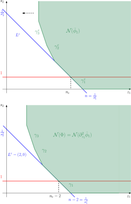
Figure 7. Comparison between ${\mathcal{N}}(\breve{\phi}_{1})$ and ${\mathcal{N}}(\Phi)$

In particular, since $n_{e}>2,$ the first edge ${\gamma}_{1}$ of ${\mathcal{N}}(\Phi)$, whose endpoints are $(B_{0},A_{0})=(n-2,0)$ and $(B_{1},A_{1}),$ where $A_{1}\geq 1,$ and the first edge ${\gamma}^{e}_{1}$ of ${\mathcal{N}}(\breve{\phi}_{1}),$ whose right endpoint is $(n,0),$ are having the same modulus of slope

(10.8) $$a_{1}=\frac{{\kappa}_{1}^{1}}{{\kappa}^{1}_{2}}=\frac{1}{n-n_{e}}.$$

Actually, a similar result holds true also for the other edges of ${\mathcal{N}}(\phi).$ To this end, let us denote by $\breve{\kappa}^{l}$ the weight associated to the $l$th edge ${\gamma}^{e}_{l}$ of ${\mathcal{N}}(\breve{\phi}_{1}).$ Then

$$a_{l}=\frac{{\kappa}_{1}^{l}}{{\kappa}^{l}_{2}}=\frac{\breve{\kappa}_{1}^{l}}{\breve{\kappa}^{l}_{2}}\geq a_{1},\qquad l=1,\dots,L.$$

In particular, in a similar way as in Subsection 7.6, by Lemma 7.4 this will now imply (for Step 1) that

(10.9) $$\frac{A_{l}-1}{a_{l}}+B_{l}+2\leq n_{e}$$

for $l=1,\dots,L.$ This is the analogue of the estimate (7.21), which had been crucial for the proof of Theorem 1.2.

One should therefore basically think of simply replacing $m$ by $n_{e}$ in our proof of Theorem 1.2 in order to get a proof of Theorem 1.9. However, this is, of course, an oversimplification, and there are also some important difference to be noticed, on which we shall concentrate subsequently.

11. Analysis in Step 1 of the resolution algorithm

11.1. $L^{2}$ - estimation of ${\mathcal{M}}_{j,k}^{\lambda}$ for the contribution by $E_{l}$

Since our arguments in Subsection 7.3 did not make use of the special form of $\breve{\phi}_{1},$ the $L^{2}$-estimates (7.9) remain valid also here.

11.2. $L^{1+{\varepsilon}}$ - estimates of ${\mathcal{M}}_{j,k}^{\lambda}$ for the contribution by $E_{l},l=1,\dots,L,$ when ${\lambda}\geq 2^{j}$

11.2.1. The case where $\tilde{\alpha}(s_{2})\not\equiv 0$

This case behaves more like a simplified version of the Step 2 - situation. We shall therefore defer its discussion to the end of Section 12.

11.2.2. The case where $\tilde{\alpha}(s_{2})\equiv 0$

Here, we can basically follow our discussion of the Step 1 - situation in Section 7. Observe first that all estimates up to (7.14) will again remain valid. However, after having applied Lemma 5.2, the identity (7.15) for $F_{j,k,|Y_{1}|\lesssim 1}({\lambda},s_{2},s_{3},y_{1})$ makes explicit use of the form of the phase $\breve{\phi}_{1},$ as well as the oscillatory integral giving $\mu_{j,k,|Y_{1}|\lesssim 1}^{\lambda}(y+{\Gamma}).$ We shall see that this part will indeed require a different discussion here. The complete phase is now given by

$$2^{-2k}\big{[}{\sigma}_{2}^{2}B(2^{-k}{\sigma}_{2})-2^{k}{\sigma}_{2}y_{2}\big{]}+\breve{\phi}_{1}(y_{1},2^{-k}{\sigma}_{2})-y_{3}$$

$$= 2^{-2k}\big{[}{\sigma}_{2}^{2}B(2^{-k}{\sigma}_{2})-2^{k}{\sigma}_{2}y_{2}\big{]}+p(y_{1},2^{-k}{\sigma}_{2})+\breve{\phi}_{\rm err}(y_{1},2^{-k}{\sigma}_{2})-y_{3}.$$

Recall also that here $Y_{1}:=2^{j}y_{1},$ so that the condition $|Y_{1}|\lesssim 1$ is equivalent to $|y_{1}|\lesssim 2^{-j}.$

But, since $p$ is $\tilde{\kappa}^{e}$-homogeneous of degree $1,$ we have

(11.1) $$p(y_{1},2^{-k}{\sigma}_{2})=2^{-k/\tilde{\kappa}^{e}_{2}}p(2^{ka_{1}}y_{1},{\sigma}_{2}).$$

And, by (10.5), we may write $2^{-k/\tilde{\kappa}^{e}_{2}}=2^{-{\varepsilon}_{0}k}2^{-2k},$ for some ${\varepsilon}_{0}>0.$ Moreover,

$$|2^{ka_{1}}y_{1}|=|2^{-j+ka_{1}}Y_{1}|\lesssim 2^{-j+ka_{1}}\leq 2^{-(j-ka_{l})},$$

and since we are on $E_{l},$ by (7.1) we have that $j-ka_{l}\gtrsim 1.$ Thus, $|2^{ka_{1}}y_{1}|\lesssim 1.$ These estimates show that the term $p(y_{1},2^{-k}{\sigma}_{2})+\breve{\phi}_{\rm err}(y_{1},2^{-k}{\sigma}_{2})$ can be absorbed into the term $2^{-2k}{\sigma}_{2}^{2}B(2^{-k}{\sigma}_{2}),$ i.e., we may assume that the complete phase is of the form

$$2^{-2k}\big{[}{\sigma}_{2}^{2}B(2^{-k}{\sigma}_{2},Y_{1})-2^{k}{\sigma}_{2}y_{2}\big{]}-y_{3},$$

where $B(2^{-k}{\sigma}_{2},Y_{1})$ has similar properties as $B(2^{-k}{\sigma}_{2}),$ in particular $|B(2^{-k}{\sigma}_{2},Y_{1})|\sim 1.$

From here on, we can thus again follow the arguments from Subsection 7.4, if we assume there that ${\omega}(y_{1})\equiv 0,$ and arrive at the same $L^{1+{\varepsilon}}$-estimates as in that subsection.

11.3. $L^{p}$ - estimation of ${\mathcal{M}}^{\tau_{l}}$ for the contribution by $E_{l},l=1,\dots,L,$ when ${\lambda}\geq 2^{j}$

The previous discussions show that also the $L^{p}$-estimates (7.17) remain valid. Since, for the summation in ${\lambda}$ of these estimates, only the condition $p>3/2$ was needed, and since the subsequent summation over all $k\leq j/a,$ with $a:=a_{l}\geq a_{1}$ works as well, we can thus eventually reduce to proving that the estimate

(11.2) $$\sum\limits_{j\gg 1}\Big{(}2^{j\big{[}(\frac{A-1}{a}+B+2)(\frac{2}{p}-1+{\varepsilon}^{\prime})-1\big{]}}+2^{j\big{[}\frac{A}{a}+B+2)(\frac{1}{p}-\frac{1}{2}+{\varepsilon}^{\prime})-1\big{]}}\Big{)}<\infty$$

still holds true.

But, by (10.9),

$$\frac{A-1}{a}+B+2\leq n_{e}\quad\text{and}\quad\frac{2}{p}-1<\frac{1}{n_{e}},$$

since $1/p<1/p_{e}=1/2+1/(2n_{e}),$ so that we may assume that the exponent of the first summand in (11.2) is strictly negative, and thus we can sum in $j.$

Similarly, by (10.8) and (10.7),

$$\frac{A}{a}+B+2\leq n_{e}+\frac{1}{a}\leq n_{e}+\frac{1}{a_{1}}=n_{e}+(n-n_{e})=n\quad\text{and}\quad\frac{1}{p}-\frac{1}{2}<\frac{1}{2n_{e}}<\frac{1}{n},$$

so that we may assume that the exponent of the second summand in (11.2) is strictly negative too and we can again sum in $j.$

11.4. $L^{p}$-estimation of ${\mathcal{M}}^{\tau_{0}}$ when ${\lambda}\geq 2^{j}$

Here we need to argue in a different way in order to see that the $L^{1+{\varepsilon}}$- estimate (7.16) still remains true.

Since $p$ is a $\tilde{\kappa}^{e}$-homogeneous polynomial function, we can write it in the form

$$p(y_{1},s_{2})=y_{1}^{n}\beta(y_{1})+s_{2}\tilde{\rho}(y_{1})+s_{2}^{2}\tilde{q}(y_{1},s_{2}),$$

where $\tilde{\rho}$ and $\tilde{q}$ are $\tilde{\kappa}^{e}$-homogeneous polynomial functions. Suppose we had $\tilde{q}(0,0)\neq 0,$ so that $\tilde{q}$ would be a constant function. Then $s_{2}^{2}\tilde{q}(y_{1},s_{2})$ would be $\tilde{\kappa}^{e}$-homogeneous of degree $2\tilde{\kappa}^{e}_{2}=1,$ which would contradict (10.5). Hence we must have $\tilde{q}(0,0)=0.$

Essentially in the same way we can show that

$$\breve{\phi}_{1}(y_{1},s_{2})=y_{1}^{n}\beta(y_{1})+s_{2}\rho(y_{1})+s_{2}^{2}q(y_{1},s_{2}),$$

with analytic functions $\rho$ and $q$ such that $q(0,0)=0.$ Thus, the complete phase can be written as

$$2^{-2k}\big{[}{\sigma}_{2}^{2}B(2^{-k}{\sigma}_{2})+{\sigma}_{2}^{2}q(y_{1},2^{-k}{\sigma}_{2})-2^{k}{\sigma}_{2}(y_{2}-\rho(y_{1})\big{]}+y_{1}^{n}\beta(y_{1})-y_{3},$$

and since we may assume that $|q|\ll 1,$ the term ${\sigma}_{2}^{2}q(y_{1},2^{-k}{\sigma}_{2})$ can again be absorbed into the first term. Thus, we can indeed now argue as in Subsection 7.4, simply replacing the term $y_{1}^{m}{\omega}(y_{1})$ in this argument by $\rho(y_{1}).$

As in Subsection 7.7, what then remains to show is that

$$\sum\limits_{j,k\gg 1:k\geq j/a_{1}}\Big{(}(2^{jn-k})^{\frac{2}{p}-1+{\varepsilon}^{\prime}}\,2^{-j}+(2^{jn})^{\frac{1}{p}-\frac{1}{2}+{\varepsilon}^{\prime}}\,2^{-j}\Big{)}<\infty.$$

But, we can now essentially follow the arguments from Subsection 7.7. For instance, in the first summand, we can first sum over all $k\geq j/a_{1}$ and arrive at the sum

$$\sum\limits_{j\gg 1}2^{j\big{[}(n-\frac{1}{a_{1}})(\frac{2}{p}-1+{\varepsilon}^{\prime})-1\big{]}}.$$

But,

$$n-\frac{1}{a_{1}}=n_{e},\quad\text{and}\quad\frac{2}{p}-1<\frac{1}{n_{e}},$$

so that by choosing ${\varepsilon}^{\prime}$ sufficiently small we can indeed sum in $j.$ The remaining arguments from Subsection 7.7 can easily be adapted in a similar way, since for $p>p_{e}$ we still have

$$n(\frac{1}{p}-\frac{1}{2})<n\frac{1}{2n_{e}}<n\frac{1}{n}=1.$$

Before we come to discuss the contributions by the homogeneous domains $D_{l},$ we need to prove a crucial lemma on multiplicities of roots.

11.5. On the condition $\tilde{A}_{1}\geq 1:$ a multiplicity lemma

Lemma 11.1 (Multiplicity Lemma).

Let $P(y_{1},y_{2})$ be a polynomial function which is ${\kappa}^{1}$-homogeneous of degree 1 and satisfies $P(y_{1},0)=y_{1}^{n-2},$ where $0<{\kappa}^{1}_{2}\leq 1.$ Define $n_{e}$ as in Figure 8, i.e.,

$$n_{e}-2=\frac{1-{\kappa}^{1}_{2}}{{\kappa}^{1}_{1}}.$$

Note that then $a:={\kappa}^{1}_{1}/{\kappa}^{1}_{2}$ is the modulus of the slope of the line $L_{1}.$ Assume that $P$ has a non-trivial real root of multiplicity strictly greater then $n_{e}-2.$

Then, either $P$ is of the form

(11.3) $$P(y_{1},y_{2})=(y_{1}-{\lambda}y_{2}^{p})^{n-2},\quad\text{where}\quad p\in{\mathbb{N}}_{>0},{\lambda}\in{\mathbb{R}}\setminus\{0\},$$

or all non-trivial real roots of $P$ have multiplicity 1, and, more precisely, $P(y_{1},y_{2})$ is of the form

$$P(y_{1},y_{2})=y_{1}^{\nu_{1}}(y_{1}^{q}-{\lambda}y_{2}^{p}),\quad\text{where}\quad p,q\in{\mathbb{N}}_{>0},q\geq 2,\frac{p}{q}=a,{\lambda}\in{\mathbb{R}}\setminus\{0\}.$$

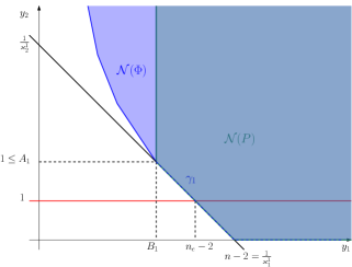
Figure 8.

Proof.

According to [IM11a, Proposition 2.2], $P$ can be written in the form

(11.4) $$P(y_{1},y_{2})=y_{1}^{\nu_{1}}\prod_{k}(y_{1}^{q}-{\lambda}_{k}y_{2}^{p})^{n_{k}},$$

with distinct ${\lambda}_{k}\in{\mathbb{C}}\setminus\{0\}$ and multiplicities $n_{k}\in{\mathbb{N}}\setminus\{0\},$ with $\nu_{1}\in{\mathbb{N}}.$

Let us put $N:=\sum\limits_{k}n_{k},$ so that $n-2=\nu_{1}+Nq,$ and note that $a=p/q.$ Note also that the monomial of lowest degree in $y_{1}$ in $P$ is then of the form $cy_{1}^{\nu_{1}}y_{2}^{Np},$ which implies that $(B_{1},A_{1})=(\nu_{1},Np).$ But then

$${\kappa}^{1}_{1}\nu_{1}+{\kappa}^{1}_{2}Np=1,\quad{\kappa}^{1}_{1}=a{\kappa}^{1}_{2},$$

hence ${\kappa}^{1}_{2}=1/(a\nu_{1}+Np).$ This implies that

(11.5) $$n_{e}-2=\frac{1-{\kappa}^{1}_{2}}{{\kappa}^{1}_{1}}=\frac{1/{\kappa}^{1}_{2}-1}{a}=\frac{a\nu_{1}+Np-1}{a}.$$

Now, by our assumption, there is some $k^{\prime}$ such that ${\lambda}_{k^{\prime}}\in{\mathbb{R}}\setminus\{0\}$ and $n_{k^{\prime}}>n_{e}-2.$ In particular, (11.5) implies that

(11.6) $$N\geq n_{k^{\prime}}>\nu_{1}+\frac{Np-1}{a},$$

hence

(11.7) $$(p-a)N<1-a\nu_{1}.$$

(i) If $q=1,$ then $a=p,$ so that by (11.7) we have $p\nu_{1}<1,$ hence $\nu_{1}=0.$ Thus, by (11.4)

$$P(y_{1},y_{2})=\prod_{k}(y_{1}-{\lambda}_{k}y_{2}^{p})^{n_{k}}.$$

But, by (11.6), $n_{k^{\prime}}>N-1/p,$ hence $n_{k^{\prime}}=N=n-2.$ This implies

$$P(y_{1},y_{2})=(y_{1}-{\lambda}_{k^{\prime}}y_{2}^{p})^{n-2}.$$

(i) If $q\geq 2,$ then by (11.7),

$$N<\frac{1-a\nu_{1}}{p-a}\leq\frac{1}{p-a}=\frac{1}{p(1-1/q)}\leq\frac{1}{p/2}=\frac{2}{p}\leq 2.$$

Thus, $N=1,$ and without loss of generality we may assume that $N=n_{1}=1.$ This implies that

$$P(y_{1},y_{2})=y_{1}^{\nu_{1}}(y_{1}^{q}-{\lambda}_{1}y_{2}^{p}),$$

hence all non-trivial real roots of $P$ are simple. Q.E.D.

11.6. On the contributions by the homogeneous domains $D_{l},l=1,\dots,L$

As in Subsection 11.6, the case $l=1$ requires special considerations. To this end, recall that the ${\kappa}^{e}$-principal part of $\breve{\phi}_{1}(z_{1},s_{2})$ is the polynomial $p(z_{1},s_{2}),$ and accordingly

$$P(z_{1},s_{2}):={\partial}_{z_{1}}^{2}p(z_{1},s_{2})$$

is the ${\kappa}^{1}$-principal part of $\Phi(z_{1},s_{2})={\partial}_{z_{1}}^{2}\breve{\phi}_{1}(z_{1},s_{2}),$ which is associated to the first edge ${\gamma}_{1}$ of ${\mathcal{N}}(\Phi).$ Moreover, if $a=a_{1},$ then every non-trivial real root of $P$ will be of the form $cs_{2}^{a},$ with $c\neq 0.$

Now, suppose again that we change in a narrow homogeneous neighborhood $D_{1}^{c}$ of this root to the coordinates $\tilde{z}:=z_{1}-cs_{2}^{a},$ so that we pass from $\Phi$ to $\tilde{\Phi}(\tilde{z},s_{2}):=\Phi(\tilde{z}+cs_{2}^{a},s_{2}),$ and from $P$ to $\tilde{P}(\tilde{z},s_{2}):=P(\tilde{z}+cs_{2}^{a},s_{2}).$

Observe first that Subcase (ii) of Case 2 from Subsection 11.6 will appear here if and only if $\tilde{P}$ will be of the form $c_{0}z_{1}^{n-2},$ i.e., if the edge ${\gamma}_{1}$ will “shrink” to its right vertex $(\tilde{B}_{0},\tilde{A}_{0})=(B_{0},A_{0})=(n-2,0)$ under the change of coordinates. But, this would mean that

$$P(z_{1},s_{2})=n(n-1)(z_{1}-cs_{2}^{a})^{n-2}.$$

However, this is excluded by our assumption (A2) (cf. (10.6)).

Thus, again, only Subcase (i) of Case 2 can appear (compare Remark 7.7 (a)), so that the first compact edge $\tilde{\gamma}_{1}$ of ${\mathcal{N}}(\tilde{\Phi})$ lies on the same line $L_{1}$ as ${\gamma}_{1}.$ Denote again by $(\tilde{B}_{0},\tilde{A}_{0})=(B_{0},A_{0})=(n-2,0)$ its right endpoint, and by $(\tilde{B}_{1},\tilde{A}_{1})$ its left endpoint. Then $\tilde{\gamma}_{1}$ is associated to $\tilde{P}.$

Assume now that we had $\tilde{\nu}_{1}=\tilde{B}_{1}>n^{e}-2,$ where $\tilde{\nu}_{1}$ denotes the power of $y_{1}$ of the first factor in (11.4), if we look at $\tilde{P}$ in place of $P.$ But that would mean that $P(z_{1},s_{2})$ would have a non-trivial real root of order strictly greater than $n^{e}-2,$ so that we could apply Lemma 11.1 to $P(z_{1},s_{2})$ and conclude that either

$$P(z_{1},s_{2})=(z_{1}-cs_{2}^{p})^{n-2},$$

(compare (11.3)), or all non-trivial real roots of $P$ have multiplicity 1. The first case is, however, again excluded by assumption (A1).

In conclusion, we see that either all of the non-trivial real roots of $P$ have multiplicity 1 (as it had been in Section 7), or we must have $\tilde{B}_{1}\leq n^{e}-2.$ But, this is equivalent to having $\tilde{A}_{1}\geq 1$ (compare Figure 8).

From here on, all of the remaining arguments from Section 7 carry over to our present situation.

12. Analysis in Step 2 of the resolution algorithm

Fixing again $l_{1}\in\{1,\dots,L\}$ as in Section 8, putting accordingly

$$a:=a_{l_{1}}\geq a_{1},$$

and proceeding in the same way as before, we are again led to considering changes of coordinates of the form

$$\tilde{z}:=z_{1}-w(s_{2}),$$

where $w(s_{2})=cs_{2}^{a}$ (or a full root $r_{0}$ with this leading term). The function $\Phi(z_{1})$ will then lead to the function $\tilde{\Phi}(\tilde{z}).$ Note, however, one difference in the effect on the function $F:$

Due to the presence of the extra term $\tilde{\alpha}(s_{2})$ in the phase for $F({\lambda},s_{2},s_{3},y_{1})$ in (10.4), we should here indeed better define $\Phi_{0}(x_{1},s^{\prime}):=\breve{\phi}_{1}(x_{1},s_{2})+s_{1}(x_{1}+\tilde{\alpha}(s_{2}))$ , and therefore

$$\tilde{\Phi}_{0,0}(\tilde{z},s_{2}) := \breve{\phi}_{1}(\tilde{z}+w(s_{2}),s_{2}),$$

$$\tilde{\Phi}_{0}(\tilde{z},s^{\prime}) := \Phi_{0}(\tilde{z}+w(s_{2}),s_{2})=\tilde{\Phi}_{0,0}(\tilde{z},s_{2})+s_{1}\tilde{z}+s_{1}\big{(}w(s_{2})+\tilde{\alpha}(s_{2})\big{)}.$$

We shall therefore also introduce the function

$$W(s_{2}):=w(s_{2})+\tilde{\alpha}(s_{2}),$$

besides the function $w(s_{2}),$ in Step 2, and similarly also in every higher order step.

Now, either $W(s_{2})\equiv 0,$ but then we can proceed in Step 2 (or higher) essentially in the same way as in Step 1, so that we shall ignore this case in the sequel.

Or, $W(s_{2})\not\equiv 0,$ and then

$$|W(s_{2})|\sim s_{2}^{a^{\prime}}$$

for some rational $a^{\prime}>0,$ since $W(s_{2})$ is fractionally analytic.

We remark that the value of $a^{\prime}$ can depend on the step of the resolution algorithm, since in higher steps of our algorithm we shall have to replace the function $w(s_{2})$ by the leading jet of some higher-order sub-cluster of roots. Observe also: since $\tilde{\alpha}(s_{2})$ is analytic, we have that $|\tilde{\alpha}(s_{2})|\sim s_{2}^{a_{0}}$ for some integer $a_{0}\geq 1.$ The following lemma is then immediate:

Lemma 12.1.

Either $a^{\prime}\geq 1,$ or $a^{\prime}<1,$ and then $a<1$ and hence $1>a^{\prime}=a\geq a_{1}.$

Next, as in Subsection 8.2, we can reduce to estimating the contributions by the $\tilde{\kappa}^{l}$- homogeneous domains $\tilde{D}_{l}$ of the form

$$\tilde{D}_{l}:=\{(\tilde{z},s_{2}):2^{-M}s_{2}^{\tilde{a}_{l}}\leq|\tilde{z}|\leq 2^{M}s_{2}^{\tilde{a}_{l}}\},\quad l\leq\tilde{L},$$

and the transition domains of the form

$$\tilde{E}_{l} := \{(\tilde{z},s_{2}):2^{M}s_{2}^{\tilde{a}_{l+1}}<|\tilde{z}|<2^{-M}s_{2}^{\tilde{a}_{l}}\},\quad l\leq\tilde{L}-1,$$

$$\tilde{E}_{\tilde{L}} := \{(\tilde{z},s_{2}):|\tilde{z}|<2^{-M}s_{2}^{\tilde{a}_{\tilde{L}}}\}.$$

More precisely, in Case 1 where $c\notin\mathcal{C}_{l_{1}},$ according to Remark 7.5 we just need the transition domain $\tilde{E}_{\tilde{L}},$ where $\tilde{L}=l_{1}.$

In Case 2, where $c\in\mathcal{C}_{l_{1}},$ we need to distinguish two subcases: if we are in Subcase (i), then according to Remark 7.6 (a) we shall need the transition domains $\tilde{E}_{l}$ with $l\geq l_{1}\geq 1$ and the homogeneous domains $\tilde{D}_{l}$ with $l\geq l_{1}+1\geq 2.$ Moreover, in analogy with Remark 8.1 (a), we may and shall treat the case where $l_{1}=1$ and where all non-trivial real roots of $P$ have multiplicity 1 separartely, so that we shall here even assume that $l_{1}\geq 2.$

In Subcase (ii) of Case 2, according to Remark 7.7 we may assume that $l_{1}\geq 2$ and shall then need the transition domains $\tilde{E}_{l}$ with $l\geq l_{1}-1\geq 1$ and the homogeneous domains $\tilde{D}_{l}$ with $l\geq l_{1}\geq 2.$

Moreover, our discussion in Subsection 11.6 shows that under these assumptions we may assume that $\tilde{A}_{1}\geq 1,$ and that the edges $\tilde{\gamma}_{1}$ and ${\gamma}_{1}$ are supported on the same line $\tilde{L}_{1}=L_{1}$ of “slope” $\tilde{a}_{1}=a_{1},$ so that, by Lemma 7.4, we now have (in analogy with the identities (8.2) and (8.3)) that

(12.1) $$\frac{\tilde{A}_{1}-1}{\tilde{a}_{1}}+\tilde{B}_{1}+2=n_{e},$$

(even when $\tilde{A}_{1}<1$), and

(12.2) $$\frac{\tilde{A}_{l}-1}{\tilde{a}_{l}}+\tilde{B}_{l}+2\leq n_{e},\quad l=1,\dots,\tilde{L}$$

(compare with (10.9)).

Having fixed $l_{1}$ and $l$ according to these assumptions, we shall put

$$\tilde{a}:=\tilde{a}_{l}.$$

Note that if we are in Case 1, or Subcase (i) of Case 2, then $\tilde{a}\geq\tilde{a}_{l_{1}}=a,$ but in Subcase (ii) it may also happen that $\tilde{a}<a$ (for instance if $l=l_{1}-1,$ where $\tilde{a}=a_{l_{1}-1}<a_{l_{1}}=a$).

12.1. Resolution of singularity on the transition domain $\tilde{E}_{l}$

Fix $\tilde{E}_{l}$ with $l\geq l_{1},$ respectively $l\geq l_{1}-1\geq 1$ if we are in the Subcase (ii) of Case 2. Arguing as in Subsection 8.3, we here find that

(12.3) $$\tilde{\Phi}_{0}(\tilde{z},s^{\prime})=\tilde{U}(\tilde{z},s_{2})s_{2}^{\tilde{A}_{l}}\tilde{z}^{\tilde{B}_{l}+2}+s_{1}(\tilde{z}+W(s_{2}))+\tilde{z}\tilde{g}(s_{2})+\tilde{h}(s_{2}).$$

And, after applying the change of coordinates $\tilde{z}=2^{-j}z,\ s_{2}=2^{-k}{\sigma}_{2}$ putting $A:=\tilde{A}_{l},B:=\tilde{B}_{l}$ and

$$d_{j,k}:=2^{-kA-j(B+2)},$$

assuming that (8.6) holds true, we obtain

$$\tilde{\Phi}_{0}^{s}(z,s_{1},{\sigma}_{2})-s_{1}y_{1}=d_{j,k}U^{s}(z,{\sigma}_{2}){\sigma}_{2}^{A}z^{B+2}+s_{1}(2^{-j}z+W(s_{2})-y_{1})+2^{-j}z\tilde{g}(s_{2})+\tilde{h}(s_{2}),$$

where $U$ has similar properties as in (7.7). Let us then write

$$W(s_{2})=2^{-ka^{\prime}}{\sigma}_{2}^{a^{\prime}}\tilde{W}({\sigma}_{2}),$$

so that $|\tilde{W}|\sim 1,$ whereas all derivatives of $\tilde{W}$ can be assumed to be very small. We shall use the following abbreviations:

$$Y_{1}: = 2^{ka^{\prime}}y_{1},$$

(12.4) $$\gamma({\sigma}_{2},Y_{1}) := {\sigma}_{2}^{a^{\prime}}\tilde{W}({\sigma}_{2})-Y_{1},$$

$$K := 2^{j-ka^{\prime}}.$$

These allow us to re-write again as in (8.10) and (8.11)

$$\tilde{\Phi}_{0}^{s}(z,s_{1},{\sigma}_{2})-s_{1}y_{1}$$

$$= d_{j,k}U^{s}(z,{\sigma}_{2}){\sigma}_{2}^{A}z^{B+2}+2^{-j}s_{1}\big{(}K{\gamma}({\sigma}_{2},Y_{1})+z\big{)}+2^{-j}z\tilde{g}(s_{2})+\tilde{h}(s_{2})$$

and

$$\tilde{F}_{j,k}({\lambda},2^{-k}{\sigma}_{2},s_{3},y_{1})=2^{-j}\iint e^{-i{\lambda}s_{3}(\tilde{\Phi}_{0}^{s}(z,s_{1},{\sigma}_{2})-s_{1}y_{1})}\chi_{0}(s_{1})\chi_{1}(z)\,\eta dzds_{1}$$

$$=2^{-j}e^{-i{\lambda}s_{3}\tilde{h}(s_{2})}\,\int{\varphi}\big{(}s_{3}{\lambda}2^{-j}[K{\gamma}({\sigma}_{2},Y_{1})+z]\big{)}$$

$$\hskip 142.26378pt\times e^{-i{\lambda}s_{3}\big{(}d_{j,k}U^{s}(z,{\sigma}_{2}){\sigma}_{2}^{A}z^{B+2}+2^{-j}z\tilde{g}(2^{-k}{\sigma}_{2})\big{)}}\chi_{1}(z)\eta dz,$$

where $z\sim 1\sim{\sigma}_{2},$ and where ${\varphi}:=\widehat{\chi_{0}}\in{\mathcal{S}}({\mathbb{R}})$ is rapidly decaying.

12.2. $L^{2}$ - estimation of ${\mathcal{M}}_{j,k}^{\lambda}$ for the contribution by $\tilde{E}_{l}$

The $L^{2}$-estimates (8.12) again remain valid here.

12.3. $L^{1+{\varepsilon}}$ - estimates of ${\mathcal{M}}_{j,k}^{\lambda}$ for the contribution by $\tilde{E}_{l}$ when ${\lambda}\geq 2^{j}$

Again, we can essentially follow the discussions from Subsection 8.3, and shall only highlight places where the arguments require modifications. Recall from (8.9) that

$$\tilde{h}(s_{2})=\breve{\phi}_{1}(w(s_{2}),s_{2}),\quad\tilde{g}(s_{2})={\partial}_{z_{1}}\breve{\phi}_{1}(w(s_{2}),s_{2}).$$

Thus, if we put again

$$\tilde{g}^{s}({\sigma}_{2}):=\tilde{g}(2^{-k}{\sigma}_{2}),\quad\tilde{h}^{s}({\sigma}_{2}):=\tilde{h}(2^{-k}{\sigma}_{2}),$$

we see that

$$\tilde{h}^{s}({\sigma}_{2})=\breve{\phi}_{1}(2^{-ka}{\sigma}_{2}^{a}\tilde{w}({\sigma}_{2}),2^{-k}{\sigma}_{2}),\quad\tilde{g}({\sigma}_{2})={\partial}_{z_{1}}\breve{\phi}_{1}(2^{-ka}{\sigma}_{2}^{a}\tilde{w}({\sigma}_{2}),2^{-k}{\sigma}_{2}).$$

But, (11.1) implies that here

$$p(2^{-ka}{\sigma}_{2}^{a}\tilde{w}({\sigma}_{2}),2^{-k}{\sigma}_{2})=2^{-k/\tilde{\kappa}^{e}_{2}}p(2^{-k(a-a_{1})}{\sigma}_{2}^{a}\tilde{w}({\sigma}_{2}),{\sigma}_{2}),$$

where $a-a_{1}\geq 0,$ and, by (10.5), $2^{-k/\tilde{\kappa}^{e}_{2}}=2^{-{\varepsilon}_{0}k}2^{-2k},$ for some ${\varepsilon}_{0}>0.$

Similarly, since ${\partial}_{y_{1}}p$ is $\tilde{\kappa}^{e}$-homogeneous of degree $1-\tilde{\kappa}^{e}_{1},$ we see that

$${\partial}_{y_{1}}p(2^{-ka}{\sigma}_{2}^{a}\tilde{w}({\sigma}_{2}),2^{-k}{\sigma}_{2})=2^{-k\frac{1-\tilde{\kappa}^{e}_{1}}{\tilde{\kappa}^{e}_{2}}}{\partial}_{y_{1}}p(2^{-k(a-a_{1})}{\sigma}_{2}^{a}\tilde{w}({\sigma}_{2}),{\sigma}_{2}).$$

And, if we again assume that $j\gtrsim k\tilde{a},$ recalling that $\tilde{a}\geq a_{1},$ we see that also

$$2^{-j}2^{-k\frac{1-\tilde{\kappa}^{e}_{1}}{\tilde{\kappa}^{e}_{2}}}\lesssim 2^{-k/\tilde{\kappa}^{e}_{2}}.$$

These estimates imply that

$$\tilde{h}^{s}({\sigma}_{2})=O(2^{-{\varepsilon}_{0}k}2^{-2k}),\quad 2^{-j}\tilde{g}^{s}({\sigma}_{2})=O(2^{-{\varepsilon}_{0}k}2^{-2k})\text{ for }j\gtrsim k\tilde{a},$$

which means that we can absorb these terms (as functions of ${\sigma}_{2}$) into the term $s_{2}^{2}B(s_{2})=2^{-2k}{\sigma}_{2}^{2}B(2^{-k}{\sigma}_{2})$ of the amplitude of the oscillatory integral (8.5).

From here on, we can simply follow the arguments for the reduction to the case $K|{\gamma}({\sigma}_{2},Y_{1})|\lesssim 1$ in Subsection 8.5.1, distinguishing now between the Subcase 2.a: ${\lambda}2^{-ka^{\prime}}\lesssim 1$, and Subcase 2.b: ${\lambda}2^{-ka^{\prime}}\gg 1,$ and replacing accordingly $a$ by $a^{\prime}$ in these steps of proof.

Note that the main difference compared to the previous discussion lies in how we get rid of the terms $\tilde{h}^{s}({\sigma}_{2})$ and $2^{-j}\tilde{g}^{s}({\sigma}_{2}),$ which turns out to be even a bit easier here than in Subsection 8.5.1.

Next, we can also easily adapt the arguments which led to (7.15) and the identity

$$\mu_{j,k,K|{\gamma}|\lesssim 1}^{\lambda}(y+{\Gamma}) = {\lambda}^{\frac{3}{2}}2^{-k}\int e^{-i{\lambda}s_{3}\big{(}\breve{\phi}_{1}(y_{1},2^{-k}{\sigma}_{2})+2^{-2k}{\sigma}_{2}^{2}B(2^{-k}{\sigma}_{2})-2^{-k}{\sigma}_{2}y_{2}-y_{3}\big{)}}$$

$$\hskip 56.9055pt\times\chi_{1}({\sigma}_{2})\chi_{1}(s_{3})\,\chi_{0}(K{\gamma}({\sigma}_{2},Y_{1}))\,\eta d{\sigma}_{2}ds_{3}.$$

But, due to (11.1), we may absorb the term $\breve{\phi}_{1}(y_{1},2^{-k}{\sigma}_{2})$ into $2^{-2k}{\sigma}_{2}^{2}B(2^{-k}{\sigma}_{2})$ within the amplitude, so that without loss of generality we may assume that

$$\mu_{j,k,K|{\gamma}|\lesssim 1}^{\lambda}(y+{\Gamma}) = {\lambda}^{\frac{3}{2}}2^{-k}\int e^{-i{\lambda}s_{3}\big{(}2^{-2k}{\sigma}_{2}^{2}B(2^{-k}{\sigma}_{2})-2^{-k}{\sigma}_{2}y_{2}-y_{3}\big{)}}$$

$$\hskip 56.9055pt\times\chi_{1}({\sigma}_{2})\chi_{1}(s_{3})\,\chi_{0}(K{\gamma}({\sigma}_{2},Y_{1}))\,\eta d{\sigma}_{2}ds_{3}.$$

This is essentially as in Subsection 8.5.1, if we assume there that ${\omega}(y_{1})\equiv 0,$ and replace $a$ by $a^{\prime}$ in these arguments.

In this way, combining all these estimates, we see that we here obtain the following analogue to estimate (8.24):

$$\|{\mathcal{M}}_{j,k}^{\lambda}\|_{1+{\varepsilon}\to 1+{\varepsilon}}\lesssim{\lambda}^{1+{\varepsilon}}2^{-j-k}+{\lambda}^{\frac{1}{2}+{\varepsilon}}2^{-j}+{\lambda}^{\frac{1}{2}+{\varepsilon}}2^{-k}+{\lambda}^{\frac{1}{2}+{\varepsilon}}2^{-ka^{\prime}}.$$

By means of interpolation with our $L^{2}$ - estimate (8.12) and summation in ${\lambda}$ we arrive then at the following analogue to (8.6): Arguing as in Subsection 7.5, we see that we can sum over all dyadic ${\lambda}$s and obtain that, for every ${\varepsilon}^{\prime}>0,$

$$\sum\limits_{{\lambda}\gg 1}\|{\mathcal{M}}_{j,k}^{\lambda}\|_{p\to p} \lesssim (d_{j,k}^{-1}2^{-k})^{\frac{2}{p}-1+{\varepsilon}^{\prime}}\,2^{-j}+(d_{j,k}^{-1})^{\frac{1}{p}-\frac{1}{2}+{\varepsilon}^{\prime}}\,2^{-j}$$

$$+ (d_{j,k}^{-1})^{\frac{1}{p}-\frac{1}{2}+{\varepsilon}^{\prime}}\,2^{-k(\frac{2}{p}-1)}2^{-j(2-\frac{2}{p})}$$

$$+ (d_{j,k}^{-1})^{\frac{1}{p}-\frac{1}{2}+{\varepsilon}^{\prime}}\,2^{-ka^{\prime}(\frac{2}{p}-1)}2^{-j(2-\frac{2}{p})}.$$

Putting again $A:=\tilde{A}_{l},B:=\tilde{B}_{l},$ we recall from (12.1) and (12.2) that

$$\frac{A-1}{\tilde{a}}+B+2\leq n_{e},\quad\text{and}\quad d_{j,k}^{-1}=2^{kA+j(B+2)}.$$

Moreover, since we are on $\tilde{E}_{l},$ by (8.6) we have $j\geq k\tilde{a}.$

This shows that we can argue in exactly the same way as in Subsection 7.6 in order to show that we can sum the first two terms on the right-hand side of (12.3) over all $k$s and $j$s such that $j\geq k\tilde{a}.$

We are thus left with showing that

(12.6) $$\sum\limits_{j,k\gg 1:j\geq k\tilde{a}}\Big{(}(d_{j,k}^{-1})^{\frac{1}{p}-\frac{1}{2}+{\varepsilon}^{\prime}}\,2^{-k(\frac{2}{p}-1)}2^{-j(2-\frac{2}{p})}+(d_{j,k}^{-1})^{\frac{1}{p}-\frac{1}{2}+{\varepsilon}^{\prime}}\,2^{-ka^{\prime}(\frac{2}{p}-1)}2^{-j(2-\frac{2}{p})}\Big{)}<\infty,$$

provided ${\varepsilon}^{\prime}>0$ is sufficiently small.

The first sum in (12.6) can be estimated in the same way as in Subsection 7.6 - we just have to replace $m$ be $n_{e}$ in the argument.

As for the second sum, note that the terms in the second sum can be estimated by the terms of the first sum, provided $a^{\prime}\geq 1.$

This leaves as with the case where $a^{\prime}<1.$ Then, by Lemma 12.1, $a^{\prime}=a\geq a_{1},$ and as before we can distinguish between the cases $\tilde{a}\geq a,$ and $\tilde{a}<a.$

In the first case, we can follow the estimates from Subsection 7.6, with $m$ replaced by $n_{e},$ and only need to verify that $(n-n_{e})a\geq 1.$ But, $a\geq a_{1}=1/(n-n_{e})$ by (10.8), so that the desired estimate holds true.

In the second case where $\tilde{a}<a,$ we can again argue as in Subsection 7.6, since we also have that $\tilde{a}\geq a_{1}.$

This completes the proof of (12.6).

12.4. $L^{p}$ - estimates of ${\mathcal{M}}_{j,k}^{\lambda}$ for the contribution by $E_{l}$ and $\tilde{E}_{l}$ when ${\lambda}<2^{j}$

Arguing in a similar way as in Subsection 8.7, we again have the $L^{2}$-estimate (8.28).

As for the $L^{1+{\varepsilon}}$-estimates, let us first look at the Step 1-situation and the contribution by $E_{l}$. Again, we shall first assume that $\tilde{\alpha}(s_{2})\equiv 0.$

Arguing in a similar way as in Subsection 8.7, we may here again assume that

$$\Phi_{0}^{s}(z,s_{1},{\sigma}_{2})-s_{1}y_{1}=-s_{1}y_{1}.$$

We can therefore adopt our discussion from Subsection 8.7 verbatim, in which we only made use of the assumption $p>3/2.$

Let us next look at the Step 2-situation and the contribution by $\tilde{E}_{l}$: By (12.3), we can here assume that

$$\tilde{\Phi}_{0}^{s}(z,s_{1},{\sigma}_{2})-s_{1}y_{1}=s_{1}2^{-ka^{\prime}}{\gamma}({\sigma}_{2},Y_{1})+\tilde{h}(s_{2}),$$

where $z\sim 1\sim{\sigma}_{2},$ with $Y_{1},K$ and ${\gamma}({\sigma}_{2},Y_{1})$ now defined by (12.4). But, the term $\tilde{h}(s_{2})$ can again be absorbed into the term $s_{2}^{2}B(s_{2})$ and shall henceforth be dropped.

We then find that

$$\tilde{F}_{j,k}({\lambda},2^{-k}{\sigma}_{2},s_{3},y_{1})=2^{-j}\,\int{\varphi}\big{(}s_{3}{\lambda}2^{-ka^{\prime}}{\gamma}({\sigma}_{2},Y_{1})\big{)}\chi_{1}(z)\eta dz,$$

where ${\varphi}:=\widehat{\chi_{0}}\in{\mathcal{S}}({\mathbb{R}})$ is rapidly decaying, and

$$\mu_{j,k}^{\lambda}(y+{\Gamma}) = {\lambda}^{\frac{5}{2}}2^{-k}\times$$

$$\iint\tilde{F}_{j,k}({\lambda},2^{-k}{\sigma}_{2},s_{3},y_{1})e^{-i{\lambda}s_{3}(s_{2}^{2}B(s_{2})-2^{-k}{\sigma}_{2}y_{2}-y_{3})}\chi_{1}({\sigma}_{2})d{\sigma}_{2}\chi_{1}(s_{3})ds_{3}.$$

Assume first that ${\lambda}2^{-ka^{\prime}}\geq 1.$ We can here argue in the same way as in Subsection 8.7, only with $a$ replaced by $a^{\prime},$ since we only made use of the assumption $p>3/2.$

Assume next that ${\lambda}2^{-ka^{\prime}}<1.$ Since we had already seen that we may assume that $\tilde{h}^{s}\equiv 0,$ we can again follow the reasoning from Subsection 8.7, and write

$$\mu_{j,k}^{\lambda}(y+{\Gamma}) = {\lambda}^{\frac{5}{2}}2^{-j-k}\times$$

$$\hskip-56.9055pt\iint e^{-i{\lambda}s_{3}(2^{-2k}{\sigma}_{2}^{2}B(2^{-k}{\sigma}_{2})-2^{-k}{\sigma}_{2}y_{2}-y_{3})}\chi_{1}({\sigma}_{2}){\varphi}\big{(}s_{3}{\lambda}2^{-ka^{\prime}}{\gamma}({\sigma}_{2},Y_{1})\big{)}\eta d{\sigma}_{2}\,\chi_{1}(s_{3})ds_{3}.$$

But note that ${\lambda}2^{-ka^{\prime}}{\gamma}({\sigma}_{2},Y_{1})={\lambda}2^{-ka^{\prime}}{\sigma}_{2}^{a^{\prime}}\tilde{W}({\sigma}_{2})-{\lambda}y_{1},$ where the first term is harmless, since ${\lambda}2^{-ka^{\prime}}\leq 1.$ Thus we may again argue as in the Step 1 situation discussed before.

This concludes our discussion of the case where ${\lambda}<2^{j}.$

12.4.1. Completion of Step 1: the case where $\tilde{\alpha}(s_{2})\not\equiv 0$

This case can be handled like a Step 2 case, where formally $a=+\infty$ and $W(s_{2}):=\tilde{\alpha}(s_{2}),$ so that $a^{\prime}=a_{0}\geq 1,$ since $a_{0}\in{\mathbb{N}}.$ We leave the details to the interested reader.

12.5. On the contributions by the homogeneous domains $\tilde{D}_{l}$

These can easily be handled in analogy to our discussions in Subsection 12.5, with the obvious modifications of the functions $W(s_{2})$ as indicated at the beginning of Section 12.

12.6. The case where $\tilde{\kappa}^{e}_{2}=0$

In view of Remark 10.1, this case behaves very much like the cases explained before where we would have stopped our resolution algorithm, after applying a change of coordinates by subtracting a complete real roots. It can therefore be handled in a similar way as we did in such situations. We leave the details to the interested reader.

13. Higher steps of the resolution algorithm and conclusion of the proof of Theorem 1.9

Here, we can again just proceed as we did in the corresponding Section 9 for the proof of Theorem 1.2; this completes the proof of Theorem 1.9.

14. Proof of the Iosevich-Sawyer-Seeger conjecture for surfaces of class ${\mathcal{A}}^{e}_{n-1}$

In this final section, we shall briefly sketch how the proof of Theorem 1.9 can be modified in order to prove the following

Proposition 14.1.

Assume that $S$ is the graph of $1+\phi,$ and accordingly $x^{0}=(0,0,1),$ where $\phi$ is analytic and of type ${\mathcal{A}}_{n-1}^{e}$. Then, if the density $\rho$ is supported in a sufficiently small neighborhood of $x^{0},$ the condition $p>\max\{3/2,h,{2n}/(n+1)\}=max\{3/2,{2n}/(n+1)\}$ is sufficient for ${\mathcal{M}}$ to be $L^{p}$-bounded.

Details are again left to the interested reader. Recall that this result will complete the proof of the Iosevich-Sawyer-Seeger conjecture for arbitrary analytic hypersurfaces in ${\mathbb{R}}^{3}.$

Proof.

We again assume that $(y_{1},y_{2})$ are line-adapted coordinates in which (1.9) and (1.11) hold true, so that

$$p(y_{1},y_{2})=y_{1}^{n}+c_{1}y_{1}y_{2}^{\beta+2},\qquad\text{with}\ \beta\in{\mathbb{N}}.$$

Since ${\partial}_{y_{1}}^{2}p(y_{1},y_{2})=n(n-1)y_{1}^{n-2},$ we now find that the first edge ${\gamma}_{1}$ of ${\mathcal{N}}(\Phi)$ has a modulus of slope $a_{1}^{\prime}$ such that $+\infty\geq a_{1}^{\prime}>a_{1}=1/(n-n_{e}).$ This first edge will intersect the line $s_{2}=1$ at a point $(n^{\prime}_{e}-2,1),$ so that $a^{\prime}_{1}=1/(n-n^{\prime}_{e}),$ and

(14.7) $$\frac{n}{2}<n_{e}<n^{\prime}_{e}\leq n.$$

In Step 1 of the resolution algorithm, we can then proceed as in the proof of Theorem 1.9, only with $a_{1}$ replaced by $a^{\prime}_{1},$ and $n_{e}$ replaced by $n^{\prime}_{e}.$ Note that now $a\geq a^{\prime}_{1},$ and $1/p-1/2<1/(2n)\leq 1/(2n^{\prime}_{e}),$ so that the discussion in Subsection 11.3 carries over directly. Similarly, since now

$$n-\frac{1}{a^{\prime}_{1}}=n-(n-n^{\prime}_{e})=n^{\prime}_{e},\quad\text{and}\quad\frac{2}{p}-1<\frac{1}{n^{\prime}_{e}},$$

also the discussion in Subsection 11.4 carries over, since now we can therein assume that $k\geq j/a^{\prime}_{1}.$

In Step 2 (and higher later on), recall that we had put $z_{1}:=y_{1}.$ We first note that here we apply changes of coordinates of the form

$$\tilde{z}:=z_{1}-w(s_{2}),$$

where now $|w(s_{2})|\sim s_{2}^{a},\quad\text{with}\quad a\geq a^{\prime}_{1}.$ It is important that the control of the functions $\tilde{g}$ and $\tilde{h}$ that we had discussed in Subsection 12.3 still works here: recall that

$$p(2^{-ka}{\sigma}_{2}^{a}\tilde{w}({\sigma}_{2}),2^{-k}{\sigma}_{2})=2^{-k/\tilde{\kappa}^{e}_{2}}p(2^{-k(a-a_{1})}{\sigma}_{2}^{a}\tilde{w}({\sigma}_{2}),{\sigma}_{2}),$$

and since $a-a_{1}\geq a^{\prime}_{1}-a_{1}>0,$ we again can conclude that $2^{-k(a-a_{1})}\lesssim 1.$ Similarly, since now $j\geq ka\geq ka^{\prime}_{1}\geq ka_{1},$ we still have that

$$2^{-j}2^{-k\frac{1-\tilde{\kappa}^{e}_{1}}{\tilde{\kappa}^{e}_{2}}}\lesssim 2^{-k/\tilde{\kappa}^{e}_{2}}.$$

Thus, we can basically proceed as before, but there is one major difference:

In our application of the Multiplicity Lemma 11.1 for the study of the contribution by the domain $D_{1},$ we can no longer exclude the first possibility (11.3), i.e., it may happen that

$$P(z_{1},s_{2})=(z_{1}-c_{1}s_{2}^{p})^{n-2},\qquad c_{1}\in{\mathbb{R}}\setminus\{0\},p\in{\mathbb{N}}_{\geq 1},$$

vanishes of maximal order $n-2$ along a nontrivial real root. Note that here we would perform a change of coordinates $\tilde{z}:=z_{1}-w(s_{2}),$ with $w(s_{2}):=c_{1}s_{2}^{a^{\prime}_{1}},$ where $a^{\prime}_{1}=p$ is a natural number, in order to pass from $\Phi$ to $\tilde{\Phi}.$ This is now an analytic change of coordinates, so that ${\mathcal{N}}(\tilde{\Phi})$ is still a Newton polyhedron (and not just Newton-Puiseux), which implies that automatically we will have $\tilde{A}_{1}\geq 1.$

However, since in the new coordinates, $\tilde{P}(\tilde{z},s_{2})=\tilde{z}^{n-2},$ the first edge $\tilde{\gamma}_{1}$ of ${\mathcal{N}}(\tilde{\Phi})$ will have a (modulus of) slope $a^{\prime\prime}_{1}$ such that $\infty\geq a^{\prime\prime}_{1}>a^{\prime}_{1}>a_{1},$ and we shall be reduced to a region of the form

$$\tilde{D}_{1}^{c_{1}}:=\{|\tilde{z}|<{\varepsilon}s_{2}^{a^{\prime}_{1}}\},$$

in which we shall again have to devise transition domains $\tilde{E}_{l}$ and homogeneous domains $\tilde{D}_{l},$ including the case $l=1.$

For all other cases in our application of Lemma 11.1, the discussion at the end of Subsection 11.6 carries over.

Now, if we proceed to higher steps of our resolution algorithm, we shall either no longer encounter the first possibility (11.3) from a certain step on, so that we can directly adapt our discussion from the proof of Theorem 1.9, or the first possibility (11.3) will arise at every Step j, within the corresponding domain $D_{1}^{(j)}.$ However, when $j$ is sufficiently large, say when $j\geq j_{0},$ then $D_{1}^{(j)}$ will contain exactly one real root, of maximal multiplicity $n-2,$ (compare the discussion in Section 9), if we consider this domain in our original coordinates $(z_{1},s_{2}),$ and we see that this root $r(s_{2})$ will have a Taylor series expansion of the form

$$r(s_{2})=c_{1}s_{2}^{a^{\prime}_{1}}+c_{2}s_{2}^{a^{\prime}_{2}}+\cdots+c_{j}s_{2}^{a^{\prime}_{j}}+\cdots,$$

with natural numbers $a^{\prime}_{1}<a^{\prime}_{2}<\cdots<a^{\prime}_{j}<\cdots,$ and real coefficients $c_{j}.$ Moreover, we may then write $\Phi(z_{1},s_{2})=V(z_{1},s_{2})(z_{1}-r(s_{2}))^{n-2},$ with $|V|\sim 1.$ As what we always did in such a situation, we can now perform the analytic change of coordinates

$$\tilde{z}:=z_{1}-r(s_{2}),$$

and find that in these new coordinates $(\tilde{z},s_{2}),$ we have

$$\tilde{\Phi}(\tilde{z},s_{2})=\tilde{V}(\tilde{z},s_{2})\tilde{z}^{n-2}.$$

As in earlier situations where we had stopped the resolution of singularities algorithm, we now see that we have arrived at a good resolution of singularities and can apply our usual arguments to prove $L^{p}$ - boundedness of ${\mathcal{M}}$ for $p>\max\{3/2,2n/(n+1)\}$ (note that here $n^{\prime}_{e}=n$ if we define $n^{\prime}_{e}$ with respect to these new coordinates).

Q.E.D.

Bibliography

- [AGV88] Arnol’d, V.I., Gusein-Zade, S.M. and Varchenko, A.N., Singularities of differentiable maps. Vol. II, Monodromy and asymptotics of integrals, Monographs in Mathematics, 83. Birkhäuser, Boston Inc., Boston, MA, 1988.
- [Bou85] Bourgain, J., Estimations de certaines fonctions maximales. C. R. Acad. Sci. Paris Sér. I Math., 301 (1985) no. 10, 499–502.
- [BDIM19] S. Buschenhenke, S. Dendrinos, I.A. Ikromov, D. Müller Estimates for maximal functions associated to hypersurfaces in with height Part I, Transactions of the American Mathematical Society, Volume 372, 2019, No. 2, pages 1363-1406.
- [Gr12] Greenblatt, M., Maximal averages over hypersurfaces and the Newton polyhedron. J. Funct. Anal., 262, (2012), 2314–2348.
- [Gr13] Greenblatt, M., boundedness of maximal averages over hypersurfaces in . Trans. Amer. Math. Soc., 365, (2013), 1875–1900.
- [IKM10] Ikromov, I. A., Kempe, M., Müller, D., Estimates for maximal functions associated to hypersurfaces in and related problems of harmonic analysis. Acta Math. 204 (2010), 151–271.
- [IM11a] Ikromov, I. A., Müller, D., On adapted coordinate systems. Trans. Amer. Math. Soc., 363 (2011), no. 6, 2821–2848.
- [IM16] Ikromov, I. A., Müller, D., Fourier restriction for hypersurfaces in three dimensions and Newton polyhedra; Annals of Mathematics Studies 194, Princeton University Press, Princeton and Oxford 2016; 260 pp.
- [IU] Ikromov, I. A.; Usmanov, S. È. On the boundedness of maximal operators associated with hypersurfaces. (Russian) Sovrem. Mat. Fundam. Napravl. 64 (2018), no. 4, 650–681. 42B25
- [ISa96] Iosevich, A. and Sawyer, E., Oscillatory integrals and maximal averages over homogeneous surfaces. Duke Math. J., 82 (1996), no. 1, 103–141.
- [ISaSe99] Iosevich, A., Sawyer, E. and Seeger, A., On averaging operators associated with convex hypersurfaces of finite type. J. Anal. Math., 79 (1999), 159–187.
- [ISa97] Iosevich, A., Sawyer, E., Maximal averages over surfaces. Adv. Math., 132 (1997), 46–119.
- [NSeW93] Nagel, A., Seeger, A. and Wainger, S., Averages over convex hypersurfaces. Amer. J. Math., 115 (1993), no. 4, 903–927.
- [PS97] Phong, D.H. and Stein, E.M., The Newton polyhedron and oscillatory integral operators. Acta Math., 179 (1997), no. 1, 105–152.
- [PSS99] Phong, D. H., Stein, E. M., Sturm, J. A., On the growth and stability of real-analytic functions. Amer. J. Math., 121 (1999), no. 3, 519-554.
- [S76] Stein, E.M., Maximal functions. I. Spherical means. Proc. Nat. Acad. Sci. U.S.A., 73 (1976), no. 7, 2174–2175.
- [S93] Stein, E. M., Harmonic analysis: Real-variable methods, orthogonality, and oscillatory integrals. Princeton Mathematical Series 43. Princeton University Press, Princeton, NJ, 1993.
- [V76] Varchenko, A. N., Newton polyhedra and estimates of oscillating integrals. Funkcional. Anal. i Priložen, 10 (1976), 13–38 (Russian); English translation in Funktional Anal. Appl., 18 (1976), 175–196.
-
[Z5]
Zimmermann, E.,
On -estimates for maximal averages over hypersurfaces
not satisfying the transversality condition. Doctoral thesis, Kiel 2014.