Overhead-Free Blockage Detection and Precoding Through Physics-Based Graph Neural Networks: LIDAR Data Meets Ray Tracing

Abstract

In this letter, we address blockage detection and precoder design for multiple-input multiple-output (MIMO) links, without communication overhead required. Blockage detection is achieved by classifying light detection and ranging (LIDAR) data through a physics-based graph neural network (GNN). For precoder design, a preliminary channel estimate is obtained by running ray tracing on a 3D surface obtained from LIDAR data. This estimate is successively refined and the precoder is designed accordingly. Numerical simulations show that blockage detection is successful with 95% accuracy. Our digital precoding achieves 90% of the capacity and analog precoding outperforms previous works exploiting LIDAR for precoder design.

I Introduction

Accurate precoding is critical to unlocking the full benefits of multiple-input multiple-output (MIMO) systems. In frequency division duplex (FDD) systems, the precoder is typically designed through a closed-loop protocol. The channel state information (CSI) is estimated at the receiver on the basis of pilot signals and fed back to the transmitter. With CSI knowledge, the transmitter is finally able to select the proper precoder. Another closed-loop protocol for precoder design is beam training, a process in which the candidate precoders are tested before selecting the optimal one. Beam training is common in millimeter wave (mmWave) systems, where the receiver cannot observe the full channel matrix because of the subspace sampling problem [1]. However, these closed-loop approaches may cause a significant communication overhead due to the high antenna number in massive MIMO links [2].

In recent literature, side information has been exploited to reduce the overhead in the precoder design process. To select the optimal precoder in mmWave, sub-6GHz band signaling has been used in [3, 4]. In [5], the authors propose to select candidate beams as a function of the vehicle’s location by inverting the fingerprinting localization process. Finally, vision-aided beam prediction has been proposed in [6, 7].

Light detection and ranging (LIDAR) is a sensor commonly used in autonomous driving. It employs a laser to scan the surrounding area and obtain a 3D point cloud. LIDAR is typically used for obstacle detection but can be also exploited to improve wireless communications. In [8], [9], a convolutional neural network (CNN) has been used to identify the optimal beams given the LIDAR data. The authors used deep learning (DL) strategies to design a reduced set of precoders to be tested during the beam training procedure. As a result, the communication overhead caused by beam training can be significantly reduced. In [10], the same problem has been solved through a federated learning approach, in which the connected vehicles collaborate to train the shared DL model. In [11], the authors integrate knowledge distillation techniques, non-local attention schemes, and curriculum training to further improve the beam selection from LIDAR data.

In this study, we address the problems of blockage detection and precoder design by completely removing the communication overhead. This is realized by exploiting side information available at the transmitter, derived from LIDAR and global positioning system (GPS) data. For blockage detection, we classify the LIDAR point cloud through a physics-based graph neural network (GNN), a DL architecture never applied in this context. For precoder design, we propose a novel joint use of LIDAR data and ray tracing never investigated before. First, we reconstruct a 3D surface representing the propagation environment from the LIDAR point cloud. Second, we obtain a preliminary channel estimate by running a ray tracing simulation on top of this surface. Third, this preliminary channel estimate is refined through a CNN, and the precoder is designed accordingly. The joint use of LIDAR data and ray tracing allows us to design the precoder with a physics-based DL strategy, differently from state-of-the-art works relying on purely data-based approaches [8]-[11]. By creating a digital twin of the channel, our strategy is agnostic about the type of precoding considered, unlike related works selecting the best analog precoder within a predefined codebook [8]-[11].

II System Model

Let us consider a point-to-point MIMO link between an $N_{T}$ antenna transmitter and an $N_{R}$ antenna receiver, in a vehicle-to-infrastructure (V2I) scenario. The transmitter is a vehicular user equipment (UE) equipped with a LIDAR and a localization system, such as GPS, while the receiver is a stationary base station (BS). We denote the transmitted signal as $\sqrt{E_{s}}\mathbf{x}\in\mathbb{C}^{N_{T}\times 1}$, where $E_{s}$ is the energy normalization factor and $\mathbf{x}$ is the precoded signal subject to the constraint $\left\|\mathbf{x}\right\|_{2}=1$. The covariance matrix of the precoded signal $\mathbf{x}$ is denoted as the transmit covariance matrix and writes as $\mathbf{Q}=\mathbb{E}\left[\mathbf{x}\mathbf{x}^{H}\right]$. Denoting the received signal as $\mathbf{y}\in\mathbb{C}^{N_{R}\times 1}$, we have $\mathbf{y}=\sqrt{E_{s}}\mathbf{H}\mathbf{x}+\mathbf{n}$ where $\mathbf{H}\in\mathbb{C}^{N_{R}\times N_{T}}$ is the channel matrix, and $\mathbf{n}\sim\mathcal{CN}\left(\mathbf{0},\sigma_{n}^{2}\mathbf{I}\right)$ is the additive white Gaussian noise (AWGN). We write the channel matrix as $\mathbf{H}=\Lambda\widetilde{\mathbf{H}}$, where the scalar $\Lambda$ contains the path loss and shadowing, while $\widetilde{\mathbf{H}}$ accounts for the small-scale fading such that $\mathbb{E}\left[\|\widetilde{\mathbf{H}}\|_{F}^{2}\right]=N_{R}N_{T}$. The achievable rate $R$ is given by

$$R=\log_{2}\det\left(\mathbf{I}+\rho\widetilde{\mathbf{H}}\mathbf{Q}\widetilde{\mathbf{H}}^{H}\right),$$ (1)

where $\rho=E_{s}\Lambda^{2}/\sigma_{n}^{2}$ is the signal-to-noise ratio (SNR).

Given a channel estimate $\widehat{\mathbf{H}}$ at the UE, two possible precoding strategies are considered: multi-stream digital precoding and analog precoding with a single radio frequency (RF) chain. In the case of multi-stream digital precoding, the transmit covariance matrix maximizing (1) is given by multiple eigenmode transmission with water-filling power allocation, which is capacity achieving in the case of perfect CSI. In the case of analog precoding, the transmit covariance matrix is $\mathbf{Q}=\mathbf{w}\mathbf{w}^{H}$, where $\mathbf{w}\in\mathbb{C}^{N_{T}\times 1}$ is the analog precoder subject to the constraint $\mathbf{w}=\left(1/\sqrt{N_{T}}\right)\left[e^{j\varphi_{1}},e^{j\varphi_{2}},\dots,e^{j\varphi_{N_{T}}}\right]^{T}$, with $\varphi_{i}\in\left[0,2\pi\right)$ denoting the $i$-th phase shift. We assume that the analog precoder $\mathbf{w}$ is chosen from a discrete Fourier transform (DFT) codebook $\mathcal{W}$, obtained by adapting the codebook proposed in [12] to $N_{X}\times N_{Y}$ uniform planar arrays (UPAs). This codebook is constructed as follows, depending on the number of quantization bits $B$ used for each phase shift $\varphi_{i}$. We introduce the matrix $\mathbf{W_{X}}$ as the first $N_{X}$ rows of the $2^{B\left(N_{X}-1\right)}\times 2^{B\left(N_{X}-1\right)}$ unitary DFT matrix. In a similar way, $\mathbf{W_{Y}}$ is defined as a function of $N_{Y}$. Thus, the codewords in $\mathcal{W}$ are given by the columns of the matrix $\mathbf{W}=\mathbf{W_{X}}\otimes\mathbf{W_{Y}}$, where $\otimes$ denotes the Kronecker product. Given a channel estimate $\widehat{\mathbf{H}}$, the precoder $\mathbf{w}^{\star}$ maximizing (1) writes as

$$\mathbf{w}^{\star}=\arg\max_{\mathbf{w}\in\mathcal{W}}\mathbf{w}^{H}\widehat{\mathbf{H}}^{H}\widehat{\mathbf{H}}\mathbf{w}.$$ (2)

Our objective is to acquire a channel estimate $\widehat{\mathbf{H}}$ at the transmitter by completely removing the communication overhead caused by traditional closed-loop protocols for CSI acquisition. This is achieved by exploiting the information from the LIDAR and the GPS sensors, which are available at each transmitter.

III LIDAR Data Processing

As a result of the LIDAR measurements, a point cloud $\mathcal{P}=\{\left(x_{i},y_{i},z_{i}\right)\}_{i=1}^{\left|\mathcal{P}\right|}$ is available at the transmitter. In this study, we use this point cloud to reconstruct a 3D surface representing the physical environment in which the transmitter and receiver are located. Based on the reconstructed 3D surface, a ray tracing simulation is locally run at the transmitter assuming that the location of the transmitting UE and receiving BS are known at the transmitter. Finally, the resulting channel paths are combined to obtain a channel estimate at the transmitter, with no communication overhead. Fig. 1 shows an example of LIDAR point cloud and the channel paths obtained by running ray tracing on the reconstructed 3D surface.

With the ray tracing simulation, we obtain $L_{RT}$ channel paths, each described by a vector of features. Specifically, the $l$-th path is characterized by the complex gain $\alpha_{l}$, the azimuth angle of arrival (AoA) $\theta_{R,l}$, the elevation AoA $\phi_{R,l}$, the azimuth angle of departure (AoD) $\theta_{T,l}$, and the elevation AoD $\phi_{T,l}$. In addition, ray tracing outputs also the line-of-sight (LoS) status of the $l$-th path as $s_{RT,l}\in\{0,1\}$. We have $s_{RT,l}=1$ if the $l$-th path is the LoS path between the UE and the BS, and $s_{RT,l}=0$ otherwise. The array steering vector $\mathbf{a}\left(\theta,\phi\right)$ of UPAs with dimensions $N_{X}\times N_{Y}$ writes as

$$\mathbf{a}\left(\theta,\phi\right)=\frac{1}{\sqrt{N_{X}N_{Y}}}\begin{bmatrix}1\\ e^{j\Omega_{X}}\\ \vdots\\ e^{j\left(N_{X}-1\right)\Omega_{X}}\\ \end{bmatrix}\otimes\begin{bmatrix}1\\ e^{j\Omega_{Y}}\\ \vdots\\ e^{j\left(N_{Y}-1\right)\Omega_{Y}}\\ \end{bmatrix},$$ (3)

where $\Omega_{X}=kd_{x}\text{sin}\left(\theta\right)\text{cos}\left(\phi\right)$ and $\Omega_{Y}=kd_{y}\text{sin}\left(\theta\right)\text{sin}\left(\phi\right)$, with $k=2\pi/\lambda$ denoting the wave number. In this study, we set the antenna spacing $d_{x}=d_{y}=\lambda/2$. Given the $L_{RT}$ channel paths derived from the ray tracing simulation and the steering vector in (3), we compute the resulting MIMO channel according to the 3D mmWave channel model [2]. The resulting narrowband channel matrix $\mathbf{H}_{RT}\in\mathbb{C}^{N_{R}\times N_{T}}$ writes as

$$\mathbf{H}_{RT}=\sqrt{N_{R}N_{T}}\sum_{l=1}^{L_{RT}}\alpha_{l}\mathbf{a}_{R}\left(\theta_{R,l},\phi_{R,l}\right)\mathbf{a}_{T}^{H}\left(\theta_{T,l},\phi_{T,l}\right),$$ (4)

which is regarded as the channel estimate derived from the ray tracing simulation.

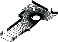
Figure 1: Example of LIDAR point cloud (left) and relative ray tracing simulation output (right).

IV Blockage Detection

mmWave technology highly relies on the presence of the LoS link to establish effective communication. Thus, it becomes crucial to assess whether the channel is in LoS or in non-line-of-sight (NLoS). We denote the channel status as $s\in\{0,1\}$, where $s=1$ means LoS and $s=0$ means NLoS. In this section, we propose three strategies to estimate the channel status $s$ given the LIDAR data.

The first strategy uses the output of the ray tracing simulation carried out as described in Section III. Let us assume that the resulting $L_{RT}$ channel paths have been ordered such that their path gains $|\alpha_{l}|$ are decreasing. We observe that among the channel paths, at most one is the LoS path with $s_{RT,l}=1$. In addition, if such a path is present, it must be the first path since longer trajectories result in lower gains. Thus, the channel status estimate $\hat{s}_{RT}$ is given by $\hat{s}_{RT}=s_{RT,1}$. We refer to this strategy as purely physics-based.

The second strategy is referred to as purely data-based since it employs a DL architecture to process the LIDAR point cloud. The blockage detection problem is formalized as a point cloud binary classification problem and solved through a GNN. We adopt a GNN since it is the only DL architecture designed to effectively deal with data lying on manifolds, point clouds, and graphs. Our GNN processes the data through a three-stage scheme. In the first stage, grouping stage, the LIDAR point cloud $\mathcal{P}$ is transformed into an undirected graph $\mathcal{G}$ by connecting each point to its $k$-nearest neighbors. In the second stage, neighborhood aggregation stage, each point aggregates information from its connected neighbors through the so-called message passing scheme. We refer to the set of points connected to the $i$-th point in $\mathcal{G}$ as the neighborhood of $i$, which is denoted as $\mathcal{N}(i)$. Furthermore, we define the position of the $i$-th point as $\mathbf{p}_{i}=[x_{i},y_{i},z_{i}]\in\mathbb{R}^{3}$. In our implementation, we consider a two-hop message passing in which the hidden features of the $i$-th point in the $\ell$-th hop, with $\ell\in\{1,2\}$, is given by

$$\mathbf{h}^{(\ell)}_{i}=\sum_{j\in\mathcal{N}(i)\cup\{i\}}\textrm{MLP1}\left(\left[\mathbf{h}_{j}^{(\ell-1)},\mathbf{p}_{j}-\mathbf{p}_{i}\right]\right),$$ (5)

where we set $\mathbf{h}_{j}^{(0)}=\mathbf{p}_{j}$. MLP1 denotes a multilayer perceptron (MLP) composed by four layers, all with 32 neurons and rectified linear unit (ReLU) activation. After the message passing process, each point holds information about its two-hop neighborhood. In the third stage, global aggregation stage, we apply a global graph readout function to aggregate all the node feature vectors $\mathbf{h}^{(2)}_{i}$, with $i=1,\ldots,\left|\mathcal{P}\right|$, into a unique graph feature vector $\mathbf{h}$. To this end, we extract $\mathbf{h}=\max\{\mathbf{h}_{1}^{(2)},\ldots,\mathbf{h}_{\left|\mathcal{P}\right|}^{(2)}\}$, where the function $\max$ takes the element-wise maximum. Finally, we apply a classifier to map the remaining features to one of the two status LoS or NLoS as $\hat{s}_{GNN}=\textrm{MLP2}\left(\mathbf{h}\right)$. MLP2 denotes a MLP composed by two layers: the first with 16 neurons and ReLU activation function; the second with one neuron and Sigmoid activation function. The output of MLP2 $\hat{s}_{GNN}$ gives the channel status estimate. To train the GNN, we minimize a loss function given by the binary cross-entropy between $\hat{s}_{GNN}$ and the ground truth $s$.

The third strategy considers the integration of both physics-based and data-based approaches, referred to as physics-based DL. To this end, we slightly modify the GNN used in our purely data-driven strategy. After the global aggregation stage, the feature vector $\mathbf{h}$ and the physics-based status estimates $\hat{s}_{RT}$ are concatenated. The resulting vector $\left[\hat{s}_{RT},\mathbf{h}\right]$ is fed in input to a new classifier MLP3 estimating the channel status as $\hat{s}_{PBGNN}=\textrm{MLP3}\left(\left[\hat{s}_{RT},\mathbf{h}\right]\right)$, where MLP3 denotes a MLP with the same structure as MLP2. Finally, $\hat{s}_{PBGNN}$ is the channel status estimate given by our physics-based GNN.

V Overhead-Free Channel Estimation

We now consider the problem of estimating the channel without communication overhead. Since our ultimate objective is to design the precoder, as discussed in Section II, it is sufficient to acquire the estimate $\widehat{\mathbf{T}}=\widehat{\mathbf{H}}^{H}\widehat{\mathbf{H}}$. We propose to compute $\widehat{\mathbf{T}}$ by refining the preliminary channel estimate derived from the ray tracing simulation. To this end, we introduce the matrix $\mathbf{T}_{RT}=\mathbf{H}_{RT}^{H}\mathbf{H}_{RT}$ with eigenvalue decomposition $\mathbf{T}_{RT}=\mathbf{V}_{RT}^{H}\mathbf{\Lambda}_{RT}\mathbf{V}_{RT}$.

To obtain $\widehat{\mathbf{T}}$, we first estimate the blockage status of the channel through the physics-based GNN strategy presented in Section IV. Then, $\widehat{\mathbf{T}}$ is computed differently for channels classified as LoS and NLoS, since these two channel types are characterized by different properties. In LoS channels, the power is mainly captured by the LoS path. Thus, they are expected to be well reconstructed by ray tracing since the reflected paths, though inaccurate, have a minimal impact. Conversely, in NLoS channels, inaccurate ray tracing might decrease the channel reconstruction quality. For this reason, we set the estimate $\widehat{\mathbf{T}}=\widehat{\mathbf{T}}_{LoS}$ if $\hat{s}_{PBGNN}\geq 1/2$ and $\widehat{\mathbf{T}}=\widehat{\mathbf{T}}_{NLoS}$ if $\hat{s}_{PBGNN}<1/2$. In the following, we illustrate how $\widehat{\mathbf{T}}_{LoS}$ and $\widehat{\mathbf{T}}_{NLoS}$ are computed.

For channels classified as LoS, we define $\mathbf{H}_{LoS}\in\mathbb{C}^{N_{R}\times N_{T}}$ as the rank-1 channel given by the LoS path between UE and BS. The channel $\mathbf{H}_{LoS}$ is computed by plugging only the LoS path into (4). Given $\mathbf{H}_{LoS}$, the channel estimate in LoS is refined by forcing the dominant eigenvector of $\mathbf{T}_{RT}$ to be the unique right eigenvector of $\mathbf{H}_{LoS}$, denoted as $\mathbf{v}_{LoS}\in\mathbb{C}^{N_{T}\times 1}$. More precisely, we set $\widehat{\mathbf{T}}_{LoS}=\widehat{\mathbf{V}}_{LoS}^{H}\widehat{\mathbf{\Lambda}}_{LoS}\widehat{\mathbf{V}}_{LoS}$, where $\widehat{\mathbf{\Lambda}}_{LoS}=\mathbf{\Lambda}_{RT}$ and $\widehat{\mathbf{V}}_{LoS}=GS([\mathbf{v}_{LoS},[\mathbf{V}_{RT}]_{:,2:N_{T}}])$. Here, $GS([\mathbf{v}_{LoS},[\mathbf{V}_{RT}]_{:,2:N_{T}}])$ denotes the Gram-Schmidt process applied to the columns of the concatenation $[\mathbf{v}_{LoS},[\mathbf{V}_{RT}]_{:,2:N_{T}}]$.

Figure 2: Proposed CNN model for channel refinement.

For channels classified as NLoS, the ray tracing estimate is refined through a CNN, applying the principle of physics-based DL. Our CNN receives in input the matrix $\mathbf{T}_{RT}$, organized as a two-channel $N_{T}\times N_{T}$ real tensor. This input is processed by a series of convolutional layers, able to capture the spatial redundancy in $\mathbf{T}_{RT}$. These layers are placed in parallel to a skip connection to avoid overfitting, as represented in Fig. 2. The hidden layers are characterized by an increasing depth, spanning from $16$ to $128$ kernels. Following each hidden layer, we place a batch normalization (BN) and a leaky rectified linear unit (LReLU) activation. The output layer has depth $2$ and linear activation, since it must approximate the difference $\mathbf{T}_{CNN}-\mathbf{T}_{RT}$, where $\mathbf{T}_{CNN}$ is the refined version of $\mathbf{T}_{RT}$ given by the CNN output. In all the layers, the kernel size is $3\times 3$, with unitary strides and zero-padding such that the output of each layer has the same size as the input. The CNN has been trained by minimizing a loss function given by the mean absolute error (MAE) between $\mathbf{T}_{CNN}$ and the ground truth $\mathbf{T}=\mathbf{H}^{H}\mathbf{H}$, which can be obtained with dedicated sampling campaigns in real-world scenarios. However, we note that imposing such a Hermitian positive semi-definite constraint to the output of a CNN is hard. Thus, we add a post-processing operation to transform $\mathbf{T}_{CNN}$ to its nearest Hermitian positive semi-definite matrix. The nearest Hermitian positive semi-definite matrix in the Frobenius norm to an arbitrary matrix $\mathbf{T}_{CNN}$ is given by $\widehat{\mathbf{T}}_{NLoS}=(\mathbf{S}+\mathbf{P})/2$, where $\mathbf{S}=(\mathbf{T}_{CNN}+\mathbf{T}_{CNN}^{H})/2$ is the nearest Hermitian matrix to $\mathbf{T}_{CNN}$, and $\mathbf{P}$ is the Hermitian polar factor of $\mathbf{S}$.

Given $\widehat{\mathbf{T}}$, the digital precoder is computed according to multiple eigenmode transmission with water-filling power allocation, while the analog precoder is selected from the codebook according to (2). Differently from beam training, the closed-loop beam selection strategy widely adopted in mmWaves, our strategy is overhead-free and enables both digital and analog precoding.

VI Numerical Results

VI-A Simulation Methodology

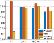
Figure 3: Performance of blockage detection solutions in terms of precision, recall, and accuracy.

To evaluate the performance of the proposed approaches, we employ the benchmark dataset Raymobtime s008 [13]. This dataset is composed of 11194 channel realizations paired with their respective LIDAR and GPS data, among which 6482 are in LoS and 4712 are in NLoS status. We build the training, validation, and test set with $80\%$, $10\%$, and $10\%$ of the samples, respectively. The antennas at the BS and at the UE are $4\times 4$ UPAs, yielding $N_{T}=N_{R}=16$. Furthermore, the DFT codebook of analog precoders has been generated by setting $B=2$, resulting in a set of $4096$ precoders. The value of $B$ has been selected to provide a good trade-off between resolution and the number of precoders. To decrease the codebook cardinality, we prune this initial codebook by retaining only the useful precoders. Specifically, we retain only the precoders that are optimal more than twice in the training set. This procedure reduces the codebook cardinality from $4096$ to $218$ possible precoders.

To reconstruct the open 3D surface we adopted the mesh-growing algorithm proposed in [14]. This algorithm proved to be particularly fast and accurate on point clouds of open surfaces. Given the 3D surface representing the environment geometry, the channel paths have been computed by employing the ray tracing propagation model available in Matlab. The shooting and bouncing rays (SBR) method has been used to calculate the channel paths with up to 6 path reflections.

The trainable parameters of the proposed DL models have been tuned by minimizing the loss function on the training set. Through cross-validation on the validation set, we have set the hyperparameters of the models characterizing their architectures, as described in Sections IV and V. Further hyperparameters have been set as follows. For the GNN employed for blockage detection, we set the neighborhood size in the graph $\mathcal{G}$ to $k=8$. We train the GNN using the Adam optimizer with learning rate $10^{-3}$ for 100 epochs, with batch size 64. The CNN employed to refine the ray tracing channel has been trained solely on the NLoS channels, using the Adam optimizer with learning rate $10^{-3}$ for 200 epochs, with batch size 200.

VI-B Performance Evaluation

We evaluate the performance of blockage detection in terms of precision, recall, and accuracy. In Fig. 3, we assess the performance of our three strategies compared with the CNN proposed in [8]. The physics-based strategy “RT” achieves an extremely high recall but a low precision. This strategy rarely classifies a LoS channel as NLoS (a false negative) since the LIDAR 3D surface rarely contain non-existing obstacles between transmitter and receiver. Conversely, it is likely to miss existing obstacles, classifying a NLoS channel as LoS (a false positive). The data-based strategy “GNN” outperforms the CNN proposed in [8]. In the physics-based DL strategy “PBGNN”, the knowledge of $\hat{s}_{RT}$ produces a twofold effect. On the one hand, $\hat{s}_{RT}$ helps the neural network to correctly classify LoS channels, increasing the recall with respect to “GNN”. On the other hand, the precision is slightly decreased since $\hat{s}_{RT}$ produces a high number of false positives. Overall, the accuracy shows that “PBGNN” outperforms “GNN”.

TABLE I: Complexity of blockage detection solutions.

Model	FLOPs		# Params.
	Aggregation net.	Classifier net.
GNN	$494\times 10^{3}$	$1.07\times 10^{3}$	$8.26\times 10^{3}$
PBGNN	$494\times 10^{3}$	$1.11\times 10^{3}$	$8.27\times 10^{3}$
[8]	$1028\times 10^{6}$		$148\times 10^{3}$

In Tab. I, we compare our strategies with [8] in terms of floating point operations (FLOPs) and trainable parameters. In GNNs, the total number of FLOPs depends on the considered point cloud since an aggregation network (implementing the two-hop message passing) is instantiated for every point in the point cloud. For this reason, we separately provide the FLOPs in the aggregation and classifier networks. In the Raymobtime s008 dataset, the average number of points in LIDAR point clouds is $E[\left|\mathcal{P}\right|]=815$, yielding approximately $403\times 10^{6}$ total FLOPs for both “GNN” and “PBGNN”, on average [13]. Thus, our blockage detection solution is attractive in terms of accuracy, computational complexity, and stored parameters.

The performance of digital precoding is evaluated considering the achievable rate $R$ as a metric. In Fig. 4, we report the performance of digital precoding based on our overhead-free channel estimation strategy “Refined”. We also report the channel capacity, achieved with perfect CSI, and the following baselines: i) “No CSI”: The transmit covariance matrix is $\mathbf{Q}=1/N_{T}\mathbf{I}$; ii) “LoS”: The precoding is based on the rank-1 LoS channel $\mathbf{H}_{LoS}$; and iii) “RT”: The precoding is based on the ray tracing channel estimate $\mathbf{H}_{RT}$. Fig. 4 shows that our channel refinement strategy outperforms the “No CSI” and “LoS” baselines. The benefit versus the “RT” strategy is visible for NLoS channels, where the CNN is used to refine the ray tracing channel estimate. Our channel refinement strategy allows achieving approximately $90\%$ of the capacity without any communication overhead in both LoS and NLoS channels.

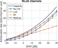
Figure 4: Achievable rate for LoS channels (left) and NLoS channels (right) obtained with digital precoding.

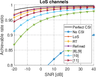
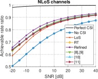
Figure 5: Achievable rate ratio for LoS channels (left) and NLoS channels (right) obtained with analog precoding.

We evaluate the performance of analog precoding considering the achievable rate ratio, defined as $\tilde{R}=R/C$, where $C=\log_{2}\left(1+\rho\lambda_{max}\right)$ is the single-stream channel capacity achieved with dominant eigenmode transmission, with $\lambda_{max}$ denoting the dominant eigenvalue of $\mathbf{T}=\mathbf{H}^{H}\mathbf{H}$. In Fig. 5, we report the performance of analog precoding based on our channel estimation strategy “Refined”. The baseline “Perfect CSI” refers to selecting the best analog precoder in the codebook for each channel realization. Conversely, for the baseline “No CSI” we always use the precoder that is most frequently optimal within the training set. We also compare our results with previous works employing LIDAR data for beam selection [8]-[11]. In the case of LoS channels, precoding based on the refined channel achieves approximately the same rate as precoding based on $\mathbf{H}_{LoS}$. In both LoS and NLoS conditions, precoding based on the refined channel outperforms precoding based on $\mathbf{H}_{RT}$ and all previous works.

In Tab. II, we report the complexity of our CNN, compared with [8]-[11]. Our solution is less complex than [8, 9] but more complex than the solutions in [10, 11]. This additional complexity is required by our solution since it explicitly estimates the MIMO channel matrix. Conversely, in [10, 11], the objective of the DL architectures is merely to select the optimal beam within a predefined codebook. Our more complex architecture brings three benefits. First, by explicitly estimating the channel, we enable precoding strategies not limited to analog precoding, e.g., digital precoding. Second, our strategy is agnostic about the considered precoding codebook. Third, our strategy achieves higher performance than previous works using the same analog precoding codebook.

TABLE II: Complexity of precoding design solutions.

Model	FLOPs	# Params.
CNN	$152\times 10^{6}$	$297\times 10^{3}$
[8, 9]	$1028\times 10^{6}$	$366\times 10^{3}$
[10]	$3.50\times 10^{6}$	$6.82\times 10^{3}$
[11]	$9.36\times 10^{6}$	$28.5\times 10^{3}$

VII Conclusion

We address the problems of blockage detection and precoder design in V2I MIMO links, by completely avoiding communication overhead. For blockage detection, we design a physics-based GNN able to correctly classify the channel status with an accuracy of 95%. For precoder design, we propose a physics-based CNN to refine a preliminary channel estimate obtained from LIDAR data. Digital precoding based on this refined channel estimate achieves 90% of the capacity while analog precoding outperforms previous related works.

References

- [1] S. Hur, T. Kim, D. J. Love, J. V. Krogmeier, T. A. Thomas, and A. Ghosh, “Millimeter Wave Beamforming for Wireless Backhaul and Access in Small Cell Networks,” IEEE Trans. Commun., vol. 61, no. 10, pp. 4391–4403, 2013.
- [2] R. W. Heath, N. González-Prelcic, S. Rangan, W. Roh, and A. M. Sayeed, “An Overview of Signal Processing Techniques for Millimeter Wave MIMO Systems,” IEEE J. Sel. Topics Signal Process., vol. 10, no. 3, pp. 436–453, 2016.
- [3] N. Gonzalez-Prelcic, A. Ali, V. Va, and R. W. Heath, “Millimeter-Wave Communication with Out-of-Band Information,” IEEE Communications Magazine, vol. 55, no. 12, pp. 140–146, 2017.
- [4] A. Ali, N. González-Prelcic, and R. W. Heath, “Millimeter Wave Beam-Selection Using Out-of-Band Spatial Information,” IEEE Trans. Wireless Commun., vol. 17, no. 2, pp. 1038–1052, 2018.
- [5] V. Va, J. Choi, T. Shimizu, G. Bansal, and R. W. Heath, “Inverse Multipath Fingerprinting for Millimeter Wave V2I Beam Alignment,” IEEE Trans. Veh. Technol., vol. 67, no. 5, pp. 4042–4058, 2018.
- [6] M. Alrabeiah, A. Hredzak, and A. Alkhateeb, “Millimeter Wave Base Stations with Cameras: Vision-Aided Beam and Blockage Prediction,” in 2020 IEEE 91st Vehicular Technology Conference (VTC2020-Spring), 2020, pp. 1–5.
- [7] G. Charan, M. Alrabeiah, and A. Alkhateeb, “Vision-Aided 6G Wireless Communications: Blockage Prediction and Proactive Handoff,” IEEE Trans. Veh. Technol., vol. 70, no. 10, pp. 10 193–10 208, 2021.
- [8] A. Klautau, N. González-Prelcic, and R. W. Heath, “LIDAR Data for Deep Learning-Based mmWave Beam-Selection,” IEEE Wireless Commun. Lett., vol. 8, no. 3, pp. 909–912, 2019.
- [9] M. Dias, A. Klautau, N. González-Prelcic, and R. W. Heath, “Position and LIDAR-Aided mmWave Beam Selection using Deep Learning,” in 2019 IEEE 20th International Workshop on Signal Processing Advances in Wireless Communications (SPAWC), 2019, pp. 1–5.
- [10] M. B. Mashhadi, M. Jankowski, T.-Y. Tung, S. Kobus, and D. Gündüz, “Federated mmWave Beam Selection Utilizing LIDAR Data,” IEEE Wireless Commun. Lett., vol. 10, no. 10, pp. 2269–2273, 2021.
- [11] M. Zecchin, M. B. Mashhadi, M. Jankowski, D. Gündüz, M. Kountouris, and D. Gesbert, “LIDAR and Position-Aided mmWave Beam Selection With Non-Local CNNs and Curriculum Training,” IEEE Trans. Veh. Technol., vol. 71, no. 3, pp. 2979–2990, 2022.
- [12] D. Love and R. Heath, “Equal gain transmission in multiple-input multiple-output wireless systems,” IEEE Trans. Commun., vol. 51, no. 7, pp. 1102–1110, 2003.
- [13] A. Klautau, P. Batista, N. González-Prelcic, Y. Wang, and R. W. Heath, “5G MIMO Data for Machine Learning: Application to Beam-Selection Using Deep Learning,” in 2018 Information Theory and Applications Workshop (ITA), 2018, pp. 1–9.
- [14] L. Di Angelo, P. Di Stefano, and L. Giaccari, “A new mesh-growing algorithm for fast surface reconstruction,” Computer-Aided Design, vol. 43, no. 6, pp. 639–650, 2011.