Geodesic bound of the minimum energy expense to achieve membrane separation within finite time

Abstract

To accomplish a task within limited operation time typically requires an excess expense of energy, whose minimum is of practical importance for the optimal design in various applications, especially in the industrial separation of mixtures for purification of components. Technological progress has been made to achieve better purification with lower energy expense, yet little is known about the fundamental limit on the least excess energy expense in finite operation time. We derive such a limit and show its proportionality to the square of a geometric distance between the initial and final states and inverse proportionality to the operation time $\tau$. Our result demonstrates that optimizing the separation protocol is equivalent to finding the geodesic curve in a geometric space. Interestingly, we show the optimal control with the minimum energy expense is achieved by a symmetry-breaking protocol, where the two membranes are moved toward each other with different speeds.

Separating components in a chemical mixture into their purer forms is critical in industrial applications (Sholl and Lively, 2016), such as water purification (Koros and Lively, 2012; Alvarez et al., 2018; Noamani et al., 2019), pharmaceutical and biological industry (van Reis and Zydney, 2007; Xie et al., 2008), and the environmental science of $\mathrm{CO}_{2}$ controls (O. Falk-Pedersen, 1997; Favre, 2007; Merkel et al., 2010; Adewole et al., 2013). The membrane separation is one of the most promising technologies due to its low energy consumption and environmental-friendly operation (Britan et al., 1991; Koros and Fleming, 1993; Spillman, 1995; Pabby et al., 2015; Castel and Favre, 2018; Purkait and Singh, 2018). Significant efforts have been made to improve the efficiency of the membranes from the perspective of material design (Pabby et al., 2015; Purkait and Singh, 2018). Nevertheless, the extent to which these properties benefit the energy expense in separation processes remains elusive. An important question arising naturally is whether there is a lower bound to the energy consumption posted by the basic laws of thermodynamics. If so, such a bound shall shed light on the material synthesis and the protocol design of separation processes.

We seek a fundamental bound of the least energy expense in finite operation time as a consequence of the basic law of thermodynamics, particularly the geometric structure of the thermal equilibrium configuration space (Weinhold, 1975; Ruppeiner, 1979; Salamon and Berry, 1983; Crooks, 2007; Sivak and Crooks, 2012; Scandi and Perarnau-Llobet, 2019; Chen et al., 2021; Li et al., 2022). For quasi-static processes with infinite operation time, the basic laws of thermodynamics have already provided a universal lower bound for the energy consumption: the performed work should exceed the free energy change of the separated final state and the mixed initial state $W\geq\Delta F$ (Callen, 1985; Huang, 1987). For a practical finite-time separation process, an excess work beyond the quasi-static separation is typically required (Huang, 1987; Tsirlin et al., 2002; Castel and Favre, 2018) and should be optimized to reach the fundamental limit (Xu and Agrawal, 1996; Tsirlin et al., 2002; Sieniutycz and Tsirlin, 2017; Sieniutycz and Jeżowski, 2018). We convert such a task of finding the minimum energy expense into finding the shortest path in a configuration space, demonstrating the first application of geometric optimization in the membrane separation process.

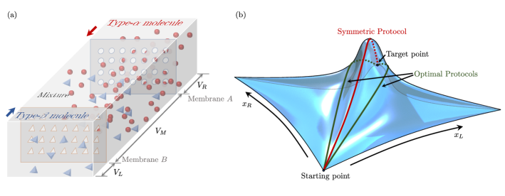
Figure 1: Separation of binary mixed gases. (a) The schematic of the separation process. The mixture consists of two types of molecules, type-$\alpha$ (red balls) and type-$\beta$ (blue triangular pyramids). The semipermeable membrane A (B) is designed for only type-$\alpha$($\beta$) to pass through. The chamber is divided into three compartments, the left one (with volume $V_{L}$) for the purified type-$\alpha$ molecules, the middle one (with volume $V_{M}$) for the molecular mixture, and the right one (with volume $V_{R}$) for the purified type-$\beta$ molecules. The two membranes are pushed towards each other during the separation process. (b) Sketch of the landscape of the configuration space spanned by $x_{k}=V_{k}/V_{t}$ ($k=L,R$) for the separation process. The metric is reflected by the surface in the three-dimensional space with an example of the equally mixed gases with symmetric diffusion coefficient. The excess work is reflected by the length of the path between the start point $\left(0,0\right)$ and the target point $\left(0.5,0.5\right)$.

Modeling the membrane separation. Consider a binary mixture of molecules in a chamber with volume $V_{t}$, as illustrated in Fig. 1(a). The system is immersed in a thermal bath with temperature $T_{0}$. Two species of the molecules are shown as red balls (type-$\alpha$) and blue triangular pyramids (type-$\beta$) with the numbers of the molecules $N_{\alpha}$ and $N_{\beta}$. The separation process is performed by mechanically moving two semipermeable membranes A and B from the two ends towards each other. The membrane A (B) is designed with the properties allowing only type-$\alpha$ (type-$\beta$) molecules to penetrate. The chamber is divided into three compartments with the two membranes: the left one with volume $V_{L}$ for the purified type-$\alpha$ molecules, the middle one with volume $V_{M}$ for the molecular mixture, and the right one with volume $V_{R}$ for the purified type-$\beta$ molecules. The three volumes satisfy the condition $V_{L}+V_{M}+V_{R}=V_{t}$. At the end of the separation, the two membranes A and B contact each other, i.e. $V_{M}=0$, and the two gases are purified in the left and the right compartments.

We denote the number of type-$\sigma$ ($\sigma=\alpha,\beta$) molecules in the compartment $k$ ($k=L,M,R$) as $N_{\sigma k}$. The impermeability of membrane A (B) to type-$\alpha$ (type-$\beta$) molecules results in $N_{\beta L}=N_{\alpha R}=0$. For the gaseous molecules, the relaxation time is far shorter than the operation time, typically referenced as the endo-reversible region (Curzon and Ahlborn, 1975; Salamon and Nitzan, 1981), where the status of the gas can be described by macroscopic parameters, i.e., the pressure and the temperature. We assume the heat exchange inside the system is fast enough to ensure a global temperature $T$ for the molecules in the whole chamber. It is worth noting that the temperature $T$ typically differs from the bath temperature $T_{0}$ due to the finite-time operation. The equation of state for the gases in each compartment is

$$p_{\sigma k}V_{k}=N_{\sigma k}k_{B}T,$$ (1)

where $k_{B}$ is the Boltzmann constant, and $p_{\sigma k}$ is the corresponding partial pressure.

Two types of relaxations exist in the separation process, the particle transport across the membranes and the heat conduction through the wall of the chamber. According to Fick’s law (Hille, 2001), the particle transport flux $\mathcal{J}_{\alpha}$ ($\mathcal{J}_{\beta}$) of type-$\alpha$ (type-$\beta$) molecules across the membrane A (B) is proportional to the particle-density difference $\Delta c_{\alpha}=N_{\alpha M}/V_{M}-N_{\alpha L}/V_{L}$ ($\Delta c_{\beta}=N_{\beta M}/V_{M}-N_{\beta R}/V_{R}$) across the membrane A (B), namely, $\mathcal{J}_{\alpha}=\mu_{\alpha}\Delta c_{\alpha}$ and $\mathcal{J}_{\beta}=\mu_{\beta}\Delta c_{\beta}$, where $\mu_{\alpha}$ ($\mu_{\beta}$) is the diffusion coefficient of the type-$\alpha$ (type-$\beta$) molecules penetrating membrane A (B). The change rates of the molecular numbers are described by $\dot{N}_{\alpha L}=\mathcal{J}_{\alpha}\mathcal{A}$ and $\dot{N}_{\beta R}=\mathcal{J}_{\beta}\mathcal{A}$, and are explicitly

$$\begin{split}\dot{N}_{\alpha L}=&\mu_{\alpha}\mathcal{A}\left(\frac{N_{\alpha M}}{V_{M}}-\frac{N_{\alpha L}}{V_{L}}\right)\,,\\ \dot{N}_{\beta R}=&\mu_{\beta}\mathcal{A}\left(\frac{N_{\beta M}}{V_{M}}-\frac{N_{\beta R}}{V_{R}}\right)\,,\end{split}$$ (2)

where $\mathcal{A}$ is the area of membranes, assumed the same for both membranes A and B. We adopt Newton’s law of cooling to describe the heat conduction between the system and the thermal bath, i.e. $\dot{Q}=-C_{V}\gamma(T-T_{0})\,$. Here $C_{V}$ is the heat capacity of the system at constant volume, e.g. $C_{V}=3/2N_{t}k_{B}$ for the ideal single-atom gas. $N_{t}=N_{\alpha}+N_{\beta}$ is the total number of the two types of molecules. $\gamma$ is the cooling rate of the system. With the first law of thermodynamics, the evolution of the gas temperature $T$ is described as

$$C_{V}\dot{T}=-C_{V}\gamma(T-T_{0})+\dot{W}\,,$$ (3)

where $\dot{W}$ is the mechanical work rate performed on the gas while moving the membranes.

Excess energy expense. To accomplish the separation, the mechanical work performed by moving the membranes is

$$W=-\int_{0}^{\tau}\sum_{\sigma=\alpha,\beta}\sum_{k=L,M,R}p_{\sigma k}\dot{V}_{k}dt\,,$$ (4)

where $\tau$ is the operation time of the separation process and $\dot{V}_{k}=dV_{k}/dt$ is the volume change rate of the compartment $k$. For convenience, we define two dimensionless parameters determining the configuration of the system, $x_{L}\equiv V_{L}/V_{t}$ and $x_{R}\equiv V_{R}/V_{t}$. The two species of molecules are completely mixed initially with $x_{L}(0)=x_{R}(0)=0$. They are separated finally with $x_{L}(\tau)$ and $x_{R}(\tau)$ satisfying $x_{L}(\tau)+x_{R}(\tau)=1$. During the separation, there is a constraint condition $0\leq x_{L}(t)+x_{R}(t)\leq 1$.

For the quasi-static separation with infinite time $\tau$, the minimum work is reached as $W_{\mathrm{min}}^{(0)}=-N_{t}k_{B}T_{0}(\epsilon_{\alpha}\ln\epsilon_{\alpha}+\epsilon_{\beta}\ln\epsilon_{\beta})$ by choosing the final volume proportional to the ratio $\epsilon_{\sigma}\equiv N_{\sigma}/N_{t}$ of the two gases, namely, $x_{L}(\tau)=\epsilon_{\alpha}$ and $x_{R}(\tau)=\epsilon_{\beta}$. See Supplementary Material for detailed discussion. For slow processes with long operation time $\tau$, the leading term of the excess work rate is a quadratic form

$$\begin{split}\dot{W}_{\mathrm{ex}}=&\frac{2N_{t}k_{B}T_{0}}{3\gamma}\left[\frac{\epsilon_{\alpha}\dot{x}_{R}}{1-x_{R}}+\frac{\epsilon_{\beta}\dot{x}_{L}}{1-x_{L}}\right]^{2}\\ &+\frac{N_{t}k_{B}T_{0}V_{t}}{\mathcal{A}}\Big{\{}\frac{\epsilon_{\alpha}(1-x_{R})}{\mu_{\alpha}}\left[\frac{d}{dt}(\frac{x_{L}}{1-x_{R}})\right]^{2}\\ &+\frac{\epsilon_{\beta}(1-x_{L})}{\mu_{\beta}}\left[\frac{d}{dt}(\frac{x_{R}}{1-x_{L}})\right]^{2}\Big{\}}\,.\end{split}$$ (5)

The first term shows the contribution due to the temperature difference between the system and the bath during the finite-time separation process. The second term shows the contribution due to the particle-density difference across the membranes A and B.

Riemann geometry of the configuration space. The quadratic form of excess work $\dot{W}_{\mathrm{ex}}$ in Eq. (5) allows the definition of a geometric length in the configuration space spanned by $(x_{L},x_{R})$. We introduce the timescale of heat transfer $\tau_{h}\equiv 1/\gamma$ and that of particle transport of type-$\sigma$ molecules $\tau_{\sigma}\equiv V_{t}/(\mu_{\sigma}\mathcal{A})$, and rewrite Eq. (5) into a compact form

$$\dot{W}_{\mathrm{ex}} =\left(\begin{array}[]{cc}\dot{x}_{L}&\dot{x}_{R}\end{array}\right)G\left(\begin{array}[]{c}\dot{x}_{L}\\ \dot{x}_{R}\end{array}\right)\,,$$ (9)

where $G$ is the metric of the current Riemann manifold

$$G=\left(\begin{array}[]{cc}g_{LL}&g_{LR}\\ g_{RL}&g_{RR}\end{array}\right)\,,$$ (10)

with the components $g_{LL}=N_{t}k_{B}T_{0}\big{[}\epsilon_{\beta}\tau_{\beta}x_{R}^{2}/(1-x_{L})^{3}+\epsilon_{\alpha}\tau_{\alpha}/(1-x_{R})+2/3\cdot\epsilon_{\beta}^{2}\tau_{h}/(1-x_{L})^{2}\big{]}\,$,$\quad g_{LR}=g_{RL}=N_{t}k_{B}T_{0}\big{[}\epsilon_{\alpha}\tau_{\alpha}x_{L}/(1-x_{R})^{2}+\epsilon_{\beta}\tau_{\beta}x_{R}/(1-x_{L})^{2}+2/3\cdot\epsilon_{\alpha}\epsilon_{\beta}\tau_{h}/(1-x_{L})(1-x_{R})\big{]}\,$,$\quad g_{RR}=N_{t}k_{B}T_{0}\big{[}\epsilon_{\alpha}\tau_{\alpha}x_{L}^{2}/(1-x_{R})^{3}+\epsilon_{\beta}\tau_{\beta}/(1-x_{L})+2/3\cdot\epsilon_{\alpha}^{2}\tau_{h}/(1-x_{R})^{2}\big{]}\,$.

The protocol of the separation process is given by $\tilde{x}_{L}(s)=x_{L}(t)$ and $\tilde{x}_{R}(s)=x_{R}(t)$ with the rescaled time $s\equiv t/\tau,\,0\leq s\leq 1$. The protocol $\tilde{x}_{L}(s)$ and $\tilde{x}_{R}(s)$ can be designed to minimize the excess work with fixed operation time $\tau$ along a given path $\mathcal{P}(x_{L},x_{R})=0$ in the configuration space. With the Cauchy-Schwarz inequality $\int_{0}^{\tau}\dot{W}_{\mathrm{ex}}dt\int_{0}^{\tau}dt\geq(\int_{0}^{\tau}\sqrt{\dot{W}_{\mathrm{ex}}}dt)^{2}\equiv\mathcal{L}^{2}$, the excess work of the given path with different protocols is bounded by

$$W_{\mathrm{ex}}\geq\frac{\mathcal{L}^{2}}{\tau}\,,$$ (11)

where the thermodynamic length $\mathcal{L}=\int_{0}^{\tau}\sqrt{\dot{W}_{\mathrm{ex}}}dt$ is only determined by the path $\mathcal{P}$ in the configuration space (Salamon and Berry, 1983; Sivak and Crooks, 2012)

$$\mathcal{L}=\int_{\mathcal{P}}\sqrt{\left(\begin{array}[]{cc}dx_{L}&dx_{R}\end{array}\right)G\left(\begin{array}[]{c}dx_{L}\\ dx_{R}\end{array}\right)}\,.$$ (12)

The equality is reached for the protocol with a constant work rate $\dot{W}_{\mathrm{ex}}=\mathrm{const}$ or a constant velocity of the thermodynamic length $d\mathcal{L}/ds=\mathrm{const}$. The task to seek the minimum energy consumption in finite time is converted into searching geodesic paths connecting the start point $(0,0)$ and the target point $(\epsilon_{\alpha},\epsilon_{\beta})$ in the configuration space.

Geodesic paths in the current Riemann manifold are described by the geodesic equations,

$$\frac{d^{2}x^{k}}{dr^{2}}+\Gamma_{\;\,ij}^{k}\frac{dx^{i}}{dr}\frac{dx^{j}}{dr}=0\,,i=1,2\,,$$ (13)

where the Einstein notation is employed, and $x^{1}\equiv x_{L},\,x^{2}\equiv x_{R}$. We parameterize the geodesic paths with the arc length $r$ by setting the initial condition $g_{ij}\frac{dx^{i}}{dr}\frac{dx^{j}}{dr}=1$. The Christoffel symbols $\Gamma_{\;\,ij}^{k}$ are obtained as $\Gamma_{\;\,ij}^{k}=\frac{1}{2}g^{kl}\left(\partial g_{li}/\partial x^{j}+\partial g_{lj}/\partial x^{i}-\partial g_{ij}/\partial x^{l}\right),$ where $g^{kl}$ are the elements of the inverse metric $G^{-1}\,$. The explicit form of $\Gamma_{\;\,ij}^{k}$ is shown in Supplementary Material.

Symmetric control path. For symmetric parameters $\tau_{\alpha}=\tau_{\beta}=\tau_{p},\epsilon_{\alpha}=\epsilon_{\beta}=0.5$, the symmetric path $x_{L}(t)=x_{R}(t)\equiv x(t)=\tilde{x}(t/\tau)$ is a geodesic path. According to Eq. (12), the thermodynamic length of the symmetric path as a function of the endpoint coordinate $x(\tau)$ is obtained as

$$\begin{split}\mathcal{L}_{s}(x(\tau))&=\int_{0}^{x(\tau)}\sqrt{g_{LL}(x,x)dx^{2}+g_{LR}(x,x)dx^{2}+g_{RL}(x,x)dx^{2}+g_{RR}(x,x)dx^{2}}\,\\ &=2\sqrt{N_{t}k_{B}T_{0}}\left.\left(\sqrt{\frac{\tau_{p}}{1-x}+\frac{2}{3}\tau_{h}}-\sqrt{\frac{2\tau_{h}}{3}}\sinh^{-1}\sqrt{\frac{2(1-x)\tau_{h}}{3\tau_{p}}}\right)\right|_{x=0}^{x(\tau)}\end{split}$$ (14)

By setting $x(\tau)=0.5$, we obtain the length of the whole path $\mathcal{L}_{\mathrm{sym}}=\mathcal{L}_{s}(0.5)\,$.

The lower bound of excess work for symmetric protocols is $\mathcal{L}_{\mathrm{sym}}^{2}/\tau$. To reach such bound, we obtain a protocol $\tilde{x}(s)$ in an implicitly form as

$$\mathcal{L}_{s}(\tilde{x}(s))=s\mathcal{L}_{\mathrm{sym}}.$$ (15)

It can be verified that $x^{1}(r)=x^{2}(r)=\tilde{x}(r/\mathcal{L}_{\mathrm{sym}})$ is a solution to the geodesic equations. We explicitly show two situations where relaxation of the particle transport or that of heat exchange dominates during the separation process.

(1) Particle transport dominated process ($\tau_{h}\ll\tau_{p}$). The temperature of the system is identical to that of the bath, $T=T_{0}$. The excess work rate is simplified as $\dot{W}_{\mathrm{ex}}=N_{t}k_{B}T_{0}\tau_{p}(1-x)\{d/dt[x/(1-x)]\}^{2}$. The thermodynamic length follows as $\mathcal{L}=(2\sqrt{2}-2)\sqrt{N_{t}k_{B}T_{0}\tau_{p}}$. According to Eq. (11), the minimum excess work is

$$W_{\mathrm{ex}}^{(\mathrm{min})}=(12-8\sqrt{2})N_{t}k_{B}T_{0}\frac{\tau_{p}}{\tau}\,.$$

The optimal protocol is designed as $\tilde{x}_{L}(s)=\tilde{x}_{R}(s)=1-[(\sqrt{2}-1)s+1]^{-2}$ to achieve the above minimum excess work.

(2) Heat exchange dominated process ($\tau_{h}\gg\tau_{p}$). The excess work rate is simplified into $\dot{W}_{\mathrm{ex}}=2/3\cdot N_{t}k_{B}T_{0}\tau_{h}[\dot{x}/(1-x)]^{2}$. The minimum excess work is

$$W_{\mathrm{ex}}^{(\mathrm{min})}=\frac{2(\ln 2)^{2}}{3}N_{t}k_{B}T_{0}\frac{\tau_{h}}{\tau}\,.$$ (16)

The designed protocol is obtained as $\tilde{x}_{L}(s)=\tilde{x}_{R}(s)=1-2^{-s}$. We summarize the two situations in Table I.

Table 1: Optimal separation protocol of equally mixed gases under the symmetric path to move two membranes. Two regions of the relaxation timescales are considered, (1) particle transport dominated process ($\tau_{h}\ll\tau_{p}$) and (2) heat exchange dominated process ($\tau_{h}\gg\tau_{p}$).

	$\tau_{h}\ll\tau_{p}$	$\tau_{h}\gg\tau_{p}$
$W_{\mathrm{ex}}^{(\mathrm{min})}$	$(12-8\sqrt{2})N_{t}k_{B}T_{0}\frac{\tau_{p}}{\tau}$	$\frac{2(\ln 2)^{2}}{3}N_{t}k_{B}T_{0}\frac{\tau_{h}}{\tau}.$
Protocol	$\tilde{x}_{L}(s)=\tilde{x}_{R}(s)=1-[(\sqrt{2}-1)s+1]^{-2}$	$\tilde{x}_{L}(s)=\tilde{x}_{R}(s)=1-2^{-s}$

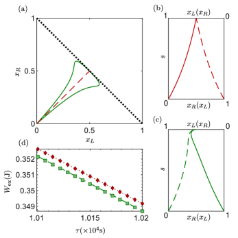
Figure 2: Symmetry-breaking protocol of the separation process with the minimum excess work. The permeable properties of membranes A and B to the corresponding type of molecules are the same, and the numbers of type-$\alpha$ and type-$\beta$ molecules are equal. Namely, all the parameters of this system are symmetric ($\tau_{\alpha}=\tau_{\beta}=1\mathrm{s},\,\tau_{h}=0.1\mathrm{s},\>\epsilon_{\alpha}=\epsilon_{\beta}=0.5,N_{t}=2N_{A},T_{0}=298.15\mathrm{K}$, where $N_{A}$ is the Avogadro constant). (a) Three geodesic paths connecting $(0,0)$ and $(0.5,0.5)$. The thermodynamic length of the two symmetry-breaking geodesic paths (green solid line) is $\mathcal{L}_{\mathrm{geo}}=59.64(\mathrm{J\cdot s})^{1/2}$, which is shorter than that of the symmetric one (red dashed line) $\mathcal{L}_{\mathrm{sym}}=59.68(\mathrm{J\cdot s})^{1/2}$. (b) and (c) Control schemes of the protocols of the symmetry-breaking and the symmetric paths. In the symmetry-breaking protocol, the two membranes approach each other at a position slightly different from the equilibrium position, and are moved together to the equilibrium position. (d) Excess work $W_{\mathrm{ex}}$ versus operation time $\tau\,$. The red diamonds (green squares) represent the irreversible work obtained by solving the evolution equation of the system along the symmetric (symmetry-breaking) path. While the red dashed line (green solid line) represents the excess work predicted by the thermodynamic length $W_{\mathrm{ex}}=\mathcal{L}^{2}/\tau$.

Symmetry breaking in the optimal separation protocol. The question arises that whether the straightforward symmetric protocol above is the optimal one with the minimum energy expense. Our answer is no. We find a symmetry-breaking protocol for the perfect symmetric setup to reach the minimum energy expense.

For given parameters, we use the shooting method (Berger, 2007) to numerically solve the geodesic path connecting the initial position $(0,0)$ and the final position $(0.5,0.5)$ in the configuration space. For room temperature $T_{0}=298.15\mathrm{K}$, we consider the symmetric situation of two moles equally mixed gases with $N_{t}=2N_{A}$, where $N_{A}$ is the Avogadro constant. The particle transport relaxation timescales are the same $\tau_{\alpha}=\tau_{\beta}=1\mathrm{s}$, and the heat conduction relaxation timescale is $\tau_{h}=0.1\mathrm{s}$. We find three geodesic paths connecting the start point $(0,0)$ and the target point $(0.5,0.5)$, shown in Fig 2(a) as the symmetric red dashed line and the two green lines. To visualize the symmetry breaking of the control scheme in the optimal separation protocol, we sketch the three-dimensional embedding of the current two-dimensional Riemann manifold in Fig. 1(b), where the thermodynamic length is reflected by the length of the path. The symmetric and the symmetry-breaking geodesic paths are shown in red and green lines. The green lines are shorter than the red one, representing smaller excess work.

The red dashed line of symmetric protocol shown in Fig 2(a) has a thermodynamic length of $\mathcal{L}_{\mathrm{sym}}=59.68(\mathrm{J\cdot s})^{1/2}$. The lengths of the symmetry-breaking green geodesic paths are $\mathcal{L}_{\mathrm{geo}}=59.64(\mathrm{J\cdot s})^{1/2}$, shorter than the symmetric one. The control schemes $\tilde{x}_{L,R}(s)$ for the symmetric and symmetry-breaking protocol are shown in Fig. 2(b) and Fig. 2(c). In the symmetry-breaking protocol shown in Fig. 2(c), the two membranes approach each other at a position different from the equilibrium position, and then are moved together to the equilibrium position. In Fig. 2(d), we compares the results obtained with the quadratic form in Eq. (5) and the numerical solution of the evolution equations (2) and (3). The red dotted line and the green dashed line show the approximate excess work predicted by thermodynamic length $W_{\mathrm{ex}}=\mathcal{L}^{2}/\tau$. And the red diamonds and the green squares present the excess work calculated with Eq. (4) by solving the evolution Eqs. (2) and (3) for the corresponding protocols $V_{L,R}(t)$ obtained from the geodesic equations.

Conclusion. We prove the equivalence between designing optimum control to achieve the minimum energy expense and finding the geodesic path in a geometric space. Such an equivalence has also been exploited in the optimization of control protocols in stochastic and quantum thermodynamics (Sivak and Crooks, 2012; Scandi and Perarnau-Llobet, 2019; Chen et al., 2021; Li et al., 2022). With this equivalence, we show the minimum excess energy expense is proportional to the square of the length of that geodesic path and inversely proportional to the operation time $\tau$. In a separation process where all the parameters are symmetric $\tau_{\alpha}=\tau_{\beta}=\tau_{p}\,,\epsilon_{\alpha}=\epsilon_{\beta}=0.5\,$, we found three geodesic paths, among them a simple and straightforward path is symmetric in the configuration space $(x_{L},x_{R})$. The corresponding protocol is to move the two membranes with the same speed. In this situation, we predict that the complete separation of equally mixed single-atom gases requires excess work at least $(12-8\sqrt{2})N_{t}k_{B}T_{0}\tau_{p}/\tau$ for the particle transport dominated process and $2(\ln 2)^{2}N_{t}k_{B}T_{0}\tau_{h}/(3\tau)$ for the heat exchange dominated process, where $\tau_{p}$ and $\tau_{h}$ are the relaxation time for the particle transport and the heat exchange.

Importantly, the current work shows that such symmetric protocol is not the best one to achieve the minimal energy expense. A symmetry-breaking protocol is the optimal protocol that achieves the lowest energy expense for given operation time $\tau$. In the optimal protocol, one membrane is moved faster than the other, the membranes approach each other at a position slightly deviated from the equilibrium position. Then they are moved together to the equilibrium position.

Acknowledgments. This work is supported by the National Natural Science Foundation of China (NSFC) (Grants No. 12088101, No. 11534002, No. 11875049, No. U1930402, No. U1930403 and No. 12047549) and the National Basic Research Program of China (Grant No. 2016YFA0301201).

Jin-Fu Chen and Ruo-Xun Zhai contributed equally to this work.

References

- Sholl and Lively (2016) David S. Sholl and Ryan P. Lively, “Seven chemical separations to change the world,” Nature 532, 435–437 (2016).
- Koros and Lively (2012) William J. Koros and Ryan P. Lively, “Water and beyond: Expanding the spectrum of large-scale energy efficient separation processes,” AIChE Journal 58, 2624–2633 (2012).
- Alvarez et al. (2018) Pedro J. J. Alvarez, Candace K. Chan, Menachem Elimelech, Naomi J. Halas, and Dino Villagrán, “Emerging opportunities for nanotechnology to enhance water security,” Nat. Nanotechnol. 13, 634–641 (2018).
- Noamani et al. (2019) Sadaf Noamani, Shirin Niroomand, Masoud Rastgar, and Mohtada Sadrzadeh, “Carbon-based polymer nanocomposite membranes for oily wastewater treatment,” npj Clean Water 2, 20 (2019).
- van Reis and Zydney (2007) Robert van Reis and Andrew Zydney, “Bioprocess membrane technology,” J. Membr. Sci. 297, 16–50 (2007).
- Xie et al. (2008) Rui Xie, Liang-Yin Chu, and Jin-Gen Deng, “Membranes and membrane processes for chiral resolution,” Chem. Soc. Rev. 37, 1243 (2008).
- O. Falk-Pedersen (1997) H. Dannström O. Falk-Pedersen, “Separation of carbon dioxide from offshore gas turbine exhaust,” Energy Conversion and Management 38, S81–S86 (1997).
- Favre (2007) Eric Favre, “Carbon dioxide recovery from post-combustion processes: Can gas permeation membranes compete with absorption?” Journal of Membrane Science 294, 50–59 (2007).
- Merkel et al. (2010) Tim C. Merkel, Haiqing Lin, Xiaotong Wei, and Richard Baker, “Power plant post-combustion carbon dioxide capture: An opportunity for membranes,” Journal of Membrane Science 359, 126–139 (2010).
- Adewole et al. (2013) J.K. Adewole, A.L. Ahmad, S. Ismail, and C.P. Leo, “Current challenges in membrane separation of CO2 from natural gas: A review,” International Journal of Greenhouse Gas Control 17, 46–65 (2013).
- Britan et al. (1991) I.M. Britan, I.L. Leites, and T.N. Vasilkovskaya, “Membrane technology of mixed-gas separation: thermodynamic analysis for feasibility study,” J. Membr. Sci. 55, 349–352 (1991).
- Koros and Fleming (1993) W.J. Koros and G.K. Fleming, “Membrane-based gas separation,” J. Membr. Sci. 83, 1–80 (1993).
- Spillman (1995) Robert Spillman, “Chapter 13 economics of gas separation membrane processes,” in Membrane Science and Technology (Elsevier, 1995) pp. 589–667.
- Pabby et al. (2015) Anil Kumar Pabby, Syed S. H. Rizvi, and Ana Maria Sastre Requena, Handbook of Membrane Separations Chemical, Pharmaceutical, Food, and Biotechnological Applications, Second Edition (Taylor and Francis Group, 2015) p. 878.
- Castel and Favre (2018) Christophe Castel and Eric Favre, “Membrane separations and energy efficiency,” J. Membr. Sci. 548, 345–357 (2018).
- Purkait and Singh (2018) Mihir K. Purkait and Randeep Singh, Membrane Technology in Separation Science (Taylor and Francis Group, 2018) p. 242.
- Weinhold (1975) F. Weinhold, “Metric geometry of equilibrium thermodynamics,” J. Chem. Phys. 63, 2479–2483 (1975).
- Ruppeiner (1979) George Ruppeiner, “Thermodynamics: A riemannian geometric model,” Phys. Rev. A 20, 1608–1613 (1979).
- Salamon and Berry (1983) Peter Salamon and R. Stephen Berry, “Thermodynamic length and dissipated availability,” Phys. Rev. Lett. 51, 1127–1130 (1983).
- Crooks (2007) Gavin E. Crooks, “Measuring thermodynamic length,” Phys. Rev. Lett. 99, 100602 (2007).
- Sivak and Crooks (2012) David A. Sivak and Gavin E. Crooks, “Thermodynamic metrics and optimal paths,” Phys. Rev. Lett. 108, 190602 (2012).
- Scandi and Perarnau-Llobet (2019) Matteo Scandi and Martí Perarnau-Llobet, “Thermodynamic length in open quantum systems,” Quantum 3, 197 (2019).
- Chen et al. (2021) Jin-Fu Chen, C. P. Sun, and Hui Dong, “Extrapolating the thermodynamic length with finite-time measurements,” Phys. Rev. E 104, 034117 (2021).
- Li et al. (2022) Geng Li, Jin-Fu Chen, C.P. Sun, and Hui Dong, “Geodesic path for the minimal energy cost in shortcuts to isothermality,” Phys. Rev. Lett. 128, 230603 (2022).
- Callen (1985) Herbert B. Callen, Thermodynamics and an Introduction to Thermostatistics, 2nd ed. (Wiley, 1985).
- Huang (1987) Kerson Huang, Statistical mechanics, 2nd ed. (Wiley, 1987).
- Tsirlin et al. (2002) Anatoliy M. Tsirlin, Vladimir Kazakov, and Dmitrii V. Zubov, “Finite-time thermodynamics: limiting possibilities of irreversible separation processes†,” J. Phys. Chem. A 106, 10926–10936 (2002).
- Xu and Agrawal (1996) Jianguo Xu and Rakesh Agrawal, “Membrane separation process analysis and design strategies based on thermodynamic efficiency of permeation,” Chem. Eng. Sci. 51, 365–385 (1996).
- Sieniutycz and Tsirlin (2017) Stanislaw Sieniutycz and Anatoly Tsirlin, “Finding limiting possibilities of thermodynamic systems by optimization,” Phil. trans. R. Soc. A 375, 20160219 (2017).
- Sieniutycz and Jeżowski (2018) Stanisław Sieniutycz and Jacek Jeżowski, “Optimization and qualitative aspects of separation systems,” in Energy Optimization in Process Systems and Fuel Cells (Elsevier, 2018) pp. 273–333.
- Curzon and Ahlborn (1975) F. L. Curzon and B. Ahlborn, “Efficiency of a carnot engine at maximum power output,” Am. J. Phys 43, 22–24 (1975).
- Salamon and Nitzan (1981) Peter Salamon and Abrahan Nitzan, “Finite time optimizations of a newton’s law carnot cycle,” J. Chem. Phys. 74, 3546–3560 (1981).
- Hille (2001) Bertil Hille, Ion Channels of Excitable Membranes (Sinauer Associates is an imprint of Oxford University Press, 2001).
- Berger (2007) Marcel Berger, A Panoramic View of Riemannian Geometry (Springer Berlin Heidelberg, 2007).