AssembleRL: Learning to Assemble Furniture
from Their Point Clouds

Abstract

The rise of simulation environments has enabled learning-based approaches for assembly planning, which is otherwise a labor-intensive and daunting task. Assembling furniture is especially interesting since furniture are intricate and pose challenges for learning-based approaches. Surprisingly, humans can solve furniture assembly mostly given a 2D snapshot of the assembled product. Although recent years have witnessed promising learning-based approaches for furniture assembly, they assume the availability of correct connection labels for each assembly step, which are expensive to obtain in practice. In this paper, we alleviate this assumption and aim to solve furniture assembly with as little human expertise and supervision as possible. To be specific, we assume the availability of the assembled point cloud, and comparing the point cloud of the current assembly and the point cloud of the target product, obtain a novel reward signal based on two measures: Incorrectness and incompleteness. We show that our novel reward signal can train a deep network to successfully assemble different types of furniture. Code and networks available here: https://github.com/METU-KALFA/AssembleRL

I Introduction

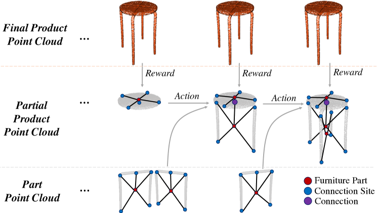
Figure 1: We propose learning to assemble a product given only its assembled form, unlike prior work that requires precise supervision for each assembly step. Our novel reward formulation uses two measures; one for measuring the incorrectness of the assembly so far, and another for the incompleteness of the assembly with respect to the target (see Fig. 4).

Assembling a product from its parts is a challenging task that fascinates kids as well as adults who prefer to build their toys/furniture from parts provided in LEGO/IKEA boxes. Although a sequence of line drawings is provided as the assembly plan of these products, the final view of the assembled product often serves as the ultimate guide, enabling humans to fill in the gaps in the assembly plans by comparing the partially assembled product with the final version. Such an assembly capability is desirable for robots to be deployed in low-volume assembly tasks, where the overhead of specifying a detailed assembly plan takes away the benefits of automation. In this sense, we are motivated by the vision of a “Assembly Robot” that you would rent to build your boxed furniture on your behalf.

In this paper, we propose a Deep Reinforcement Learning (DRL) based method, AssembleRL, to learn assembly plans using the final view of the assembled furniture as a guide, along with the specifications and view of its parts (Fig. 1). Our work, along with prior studies [1, 2] on learning-based furniture assembly, are motivated by the availability of the IKEA furniture assembly simulation environment [3] which also includes a library of furniture models.

In this paper, in contrast to prior work [1], we propose to use only the fully assembled point cloud of the furniture and the mesh models of its parts, to learn the assembly plan. Specifically, we introduce a novel reward function that evaluates the match between the point cloud of the partially assembled furniture against its fully assembled view using two measures that evaluate the incorrectness and incompleteness. We train a graph-convolutional neural network with our novel reward signal, combining the incorrectness and incompleteness measures, to learn the assembly plan as a policy that predicts which part pairs need to be connected via which of their connections. The method is successfully tested on 11 IKEA furniture models.

Our main contributions are: (1) We only use the target point cloud to learn assembly plans. (2) We introduce a novel reward function that quantifies incorrectness and incompleteness of the current assembly with respect to the target model. (3) We apply our solution to learning assembly plans for different furniture.

II Related Work and Background

Assembling with robots requires solving three main tasks [4, 5]: Modelling, planning and execution. Modelling pertains to obtaining a representation of the assembly process and includes representing parts, tools, actions etc. A common approach for assembly modelling is using graphs (e.g. [6, 2, 7, 8]), as they are naturally suitable for representing entities and the relations among them.

Assembly planning is finding a sequence of assembly actions that, once executed, lead to the assembled product is an NP-complete problem [9]. Although various backward or forward planners can be used for finding assembly plans, they generally require constraints about the task (provided by a human expert) and the resulting plan can be sub-optimal [10, 11, 12]. Therefore, in practice, human experts are needed either for creating the whole assembly plan or for collaborative assembly planning/execution [10, 13]. Automatic discovery of such plans, with little supervision, would benefit the development of “Assembly Robots”.

II-A Learning to Assemble Furniture

The rise of learning-based approaches, especially DRL, has led to unprecedented success in programming and controlling robots (see e.g. [14] for a review), which have motivated such approaches for solving assembly tasks as well. As learning an assembly with a real robot can be costly, generally simulation environments are used by learning-based assembly approaches [1, 3, 15].

It has been shown that rotation and translation between object parts can be learned to assemble objects. For this purpose, deep networks such as Convolutional Neural Networks (CNN) [16] or Graph Convolutional Networks (GCN) [17] can be used. Such networks are trained using supervised learning with Chamfer Distance between the target and the assembled parts, L2 loss of the part translations and Chamfer Distance between whole assembled product with the target assembly as the supervision signal [17] or RL using correct connection labels as the supervision signal [1].

The introduction of furniture assembly simulation environments [1, 3, 15] has enabled the use of learning-based approaches. For example, Huang et al. [17] used supervised learning to train a graph neural network to estimate 6D pose for each part to assemble chairs, lamps and tables. Yu et al. [1] employed DRL for chair assembly, though they assumed the availability of strong supervision (correct vs. incorrect labels for connections) for each assembly action.

II-B Comparative Summary

Although there are promising learning-based approaches for furniture assembly, as listed in Table I, we see that they assume the availability of strong supervision (correct vs. incorrect connection labels) for each assembly step. In contrast, in this work, we only assume the availability of point cloud of the fully assembled furniture to provide weak supervision (reward) signal to train a DRL network.

TABLE I: Learning-based approaches for furniture assembly.

Study	Method	Weak-supervision	Output
Huang et al. [17]	GNN, Supervised	✗	6D pose for each part
Yu et al. [1]	RL	✗	Pair, Connection Site, Rotation
AssembleRL	GNN, RL	✓	Pair, Connection Site

III Methodology

III-A Problem Definition

We define the problem as the discovery of an assembly plan using the fully assembled point cloud view of the furniture, along with the connection specifications and the mesh models of its parts, which are sampled to obtain point cloud representations. Specifically, let us use $P^{T}$ to denote the point cloud of the fully assembled furniture, and $P^{0}$ & $P^{t}$ to denote respectively the point cloud of the ‘seed’ part at the beginning of the assembly, and the partially assembled furniture at step $t$ of the assembly.

We assume that the assembly process starts with a single ‘seed’ part, which is grown through the attachment of other parts towards the final product. Furniture that require the assembly of separate parts, such as assembly of drawers in a separate plan, which are then attached to the body of a chest, are not addressed.

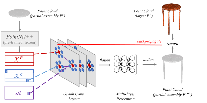
Figure 2: An overview of the proposed system. Point cloud of the current assembly ($P^{t}$) is processed by a graph neural network. The selected action is rewarded by comparing the updated assembly ($P^{t+1}$) with the target $P^{T}$.

III-B Overview

We use DRL (Proximal Policy Optimization [18] to be specific) to find a policy $\pi$ for successful assembly of furniture. Following similar studies [2, 16, 17], we use graphs to encode the state of the environment (Sect. III-C) and devise a GNN to obtain a probability distribution over the actions for successful assembly (Fig. 2 and Sect. III-D). To train the network, we propose a novel reward function (Sect. III-E) that consists of two measures: Incorrectness and Incompleteness, which are computed by matching $P^{t}$ and $P^{T}$. See Fig. 2 for an overview.

III-C Graph Representation of Assembly State

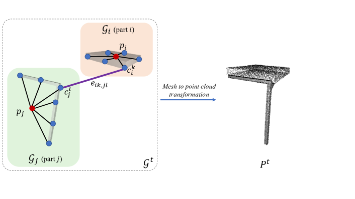
Figure 3: Each part is represented by a graph ($\mathcal{G}_{\cdot}$), consisting of a part node ($p_{\cdot}$ – red circle) and 6 connection nodes ($c_{\cdot}$ – blue circle). Parts are attached by drawing edges ($e_{\cdot}$) between connection nodes. $P^{t}$ is obtained by sampling the connected parts.

The state of the assembly is represented as a graph. Initially, each of the $N$ parts to be assembled is represented as a separate undirected graph. Specifically, the $i^{th}$ part is represented as a graph $\mathcal{G}_{i}=(p_{i},c_{i}^{1},c_{i}^{2},..,c_{i}^{6})$ consisting of a part node ($p_{i}$) attached to $6$ connection nodes ($c_{i}^{1},..,c_{i}^{6}$), shown as red and blue nodes respectively in Fig. 3. The representation of a part node $p_{i}$, denoted by $\phi(p_{i})$, is the point cloud representation for the part, whereas a connection node $c_{i}^{k}$ is represented by a one-hot vector, denoted by $\phi(c_{i}^{k})$.

Assembly actions are represented as a tuple $(\mathcal{G}_{i},\mathcal{G}_{j},c_{i}^{k},c_{j}^{l})$, where $\mathcal{G}_{i},\mathcal{G}_{j}$ represent the parts, and $c_{i}^{k},c_{j}^{l}$ represent the connection sites on these parts. An assembly action would merge $\mathcal{G}_{i},\mathcal{G}_{j}$ by adding an edge, $e_{ik,jl}$, connecting the $k^{th}$ connection site of part $i$ with the $l^{th}$ connection site of part $j$.

One of the parts, say $\mathcal{G}_{i}$, is picked as the ‘seed’ and is used to initialize the partial assembly graph denoted with $\mathcal{G}^{0}=\mathcal{G}_{i}$. The state of the partial assembly at step $t$, denoted as $\mathcal{G}^{t}$, is updated at every assembly step by merging the graph representations of other parts through edges formed by connections.

At step $t$, an action tuple $(\mathcal{G}_{i},\mathcal{G}_{j},c_{i}^{k},c_{j}^{l})$ is considered valid if (i) one of $\mathcal{G}_{i}$, $\mathcal{G}_{j}$ is a subset of $\mathcal{G}^{t}$, the partial assembly, while the other is not a subset of $\mathcal{G}^{t}$, and (ii) $e_{ik,jl}\not\in\mathcal{G}^{t}$. All other actions are considered invalid.

The state of the assembly $\mathcal{G}^{t}$ is then converted into a representation suitable to be fed to neural networks, as shown in Fig. 2. Specifically, a feature matrix, $\mathcal{X}\in\mathbb{R}^{(N+6N)\times 256}$, is used to store a processed representation of the $N$ parts and the $6N$ connections sites. For each part node $p_{i}$, its point cloud $\phi(p_{i})$ is fed into PointNet++ [19] pretrained on ModelNet [20] to compute a feature vector $\mathcal{X}_{i}\in\mathbb{R}^{256}$. The $6N$ connection sites of all $N$ parts are represented as one-hot vectors. For example, connection site ${c_{i}^{k}}$ is represented with a $1$ at position $6i+k$. In our study, the size of one-hot vector, $6N$, did not exceed the size of geometric feature vector $256$ and to be compatible with part features, the remaining dimensions are padded with zeros. Finally, the connectivity of the undirected graph $\mathcal{G}^{t}$ is represented as an adjacency matrix, $\mathcal{A}\in\mathbb{R}^{(N+6N)\times(N+6N)}$.

III-D Graph Neural Network

We constructed a deep network that consists of a graph convolutional subnetwork (GNN), followed by a multi-layer perceptron (MLP):

$$\mathcal{P}=\text{MLP}(\text{GNN}(\mathcal{X},\mathcal{A})),$$ (1)

where, as introduced in Sect. III-C, $\mathcal{X}$ is the feature matrix representing the nodes, and $\mathcal{A}$ is the adjacency matrix. For GNN, we used three layers of graph convolution operator (denoted by GCo) from [21] which modulates node features of a part with respect to other parts through the connected nodes of the connection sites:

$$\footnotesize\text{GNN}(\mathcal{X},\mathcal{A})=\text{ReLU}(\text{GCo}(\text{ReLU}(\text{GCo}(\text{ReLU}(\text{GCo}(\mathcal{X},\mathcal{A})),\mathcal{A})),\mathcal{A})),$$ (2)

where ReLU is a rectified linear unit. $\text{GNN}(\mathcal{X},\mathcal{A})$ yields $\mathcal{Z}\in\mathbb{R}^{(N+6N)\times 256}$ as the processed feature matrix. This feature matrix is ‘flattened’ and provided to $\text{MLP}(\cdot)$ as input.

$\text{MLP}(\cdot)$ is a multi-layer perceptron with two hidden layers to estimate log probabilities of each action:

$$\text{MLP}(\mathbf{x})=\text{FC}(\text{ReLU}(\text{FC}(\text{ReLU}(\text{FC}(\mathbf{x}))))),$$ (3)

where FC is a fully-connected layer.

III-E Reward Function

Reward is computed using only the point cloud of the fully assembled furniture $P^{T}$ (as summarized in Alg. 1). Unlike [1, 17], ground truth information about the connections between connection site pairs and relative part poses are not assumed, making the problem setting more practical yet more challenging.

Algorithm 1 The proposed reward function.

Input: $P^{t}$: Point cloud of partial assembly,
         $P^{T}$: Point cloud of target assembly,
         $d^{t-1}$: $\mu_{cmp}$ measure at $(t-1)$.
Output: $Reward$: Reward at the end of step,
           $Termination$: Termination condition.

$Termination\leftarrow false$

if $\mathcal{G}_{i},\mathcal{G}_{j}\nsubseteq\mathcal{G}^{t}$ then $\triangleright$ Invalid: Neither part is in partial assembly

    $Reward\leftarrow-10$, $Termination\leftarrow true$

else if $\mathcal{G}_{i},\mathcal{G}_{j}\subset\mathcal{G}^{t}$ then $\triangleright$ Invalid: Parts are already assembled

    $Reward\leftarrow-1$

else

    $d^{t}=\mu_{cmp}(P^{t},P^{T})$ $\triangleright$ Eq. 4

    if $d^{t}\geq d^{t-1}$ then $\triangleright$ Completeness $\downarrow$

       $Reward\leftarrow-10$, $Termination\leftarrow true$

    else

       if $\mu_{cor}(P^{t},P^{T})<n_{th}$ then $\triangleright$ $n_{th}$: threshold

          $Reward\leftarrow 5$ $\triangleright$ Correctness $\uparrow$

       else

          $Reward\leftarrow-5$ $\triangleright$ Correctness $\downarrow$

       end if

    end if

end if

return $Reward,Termination$

Point cloud of partial assembly, $P^{t}$, is generated from the current state of the assembly, represented in $\mathcal{G}^{t}$ and is updated after every action. To obtain $P^{t}$, at first, the mesh of the part assembly is obtained; and then a fixed number of points are sampled from this mesh. For each $P^{t}$, the same number of points are sampled, resulting in a density change after addition of new parts. The affect of the density change is discussed in the following section.

The partial assembly, $P^{t}$, is then compared against $P^{T}$ using two evaluation measures inspired from Chamfer Distance; namely incompleteness and incorrectness (Fig. 4). The incompleteness measure is designed to measure the completion progress of the partial assembly towards the final furniture, whereas the incorrectness measure aims to measure the degree of incorrect part assembling.

In order to discount the effect of the arbitrary pose of the partial assembly during its comparison with the final assembly, Iterative Closest Point (ICP) [22] is used for the point cloud registration between $P^{t}$ and $P^{T}$. Unassembled parts are excluded during the registration step and metric computation that follows it.

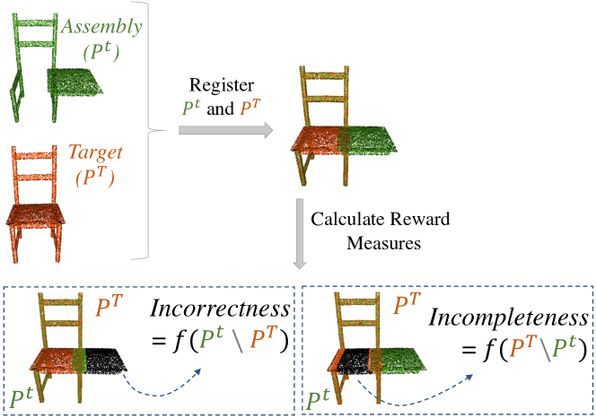
Figure 4: An illustration of the two reward measures proposed in our paper.

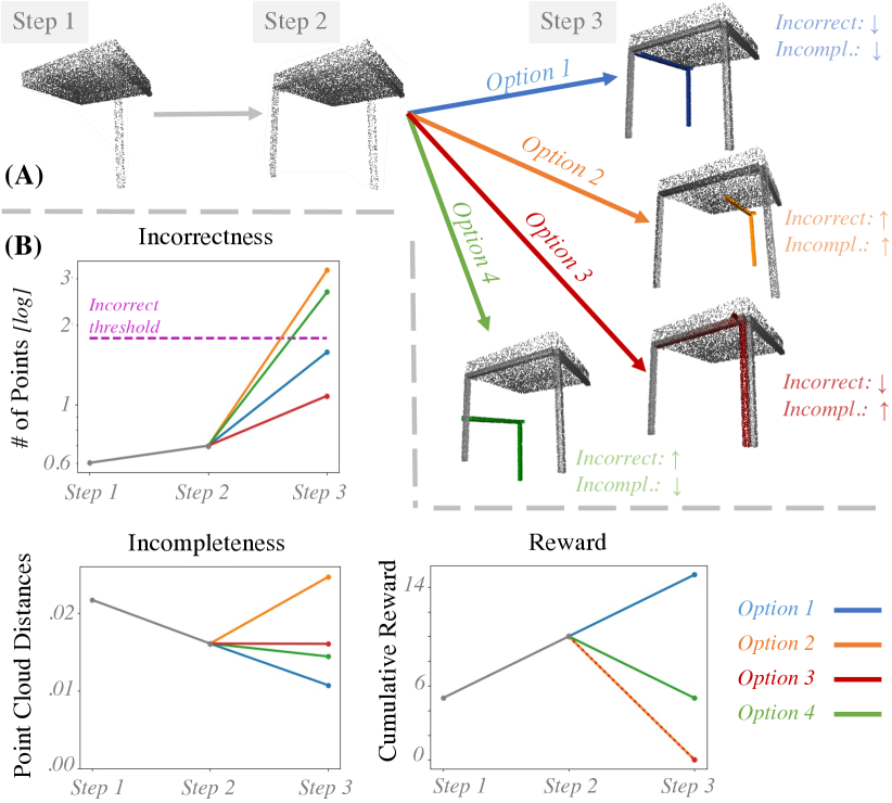
Figure 5: An illustration showing how the proposed measures and the reward values change over time. (a) Assembly of a table with three steps. (b) How different assembly actions (options in (a)) affect the measures.

The incompleteness measure is defined as the average distance from $P^{T}$ to $P^{t}$ as:

$$\mu_{cmp}(P^{T},P^{t})=\dfrac{1}{|P^{T}|}\sum_{x\in P^{T}}\min_{y\in P^{t}}||x-y||^{2}_{2},$$ (4)

where $x\in P^{T}$ and $y\in P^{t}$, are points in the point clouds of the fully and partially assembled furniture. The calculation is normalized with the number of points in the fully assembled furniture, denoted with $|P^{T}|$. The measure is expected to decrease as the assembling progresses correctly (see Fig. 5), but is not expected to drop to complete zero.

A correct assembly action would certainly reduce the average distance between paired points of the two point clouds. An incorrect assembly action, however, may result in two possible changes on the measure. If the incorrectly assembled part hampers ICP-based registration in the previous step, it would lead to an increase in the measure, as expected. However, if the assembled part fails to hamper ICP-based registration, then the points in $P^{T}$ will still be paired to the same or close-by points in in $P^{t}$, not causing a noticable increase in the measure. Moreover, the assembly of a new part into the partial assembly would increase the surface area and would make the point cloud sampled from the mesh sparser in the areas that match $P^{T}$. As a result, the measure may even decrease unexpectedly.

The unexpected behavior of the incompleteness measure is compensated by the incorrectness measure, which is defined as:

$$\mu_{cor}(P^{t},P^{T})=\sum_{x\in P^{t}}\mathbb{1}\left(\min_{y\in P^{T}}||x-y||^{2}_{2}>d_{th}\right),$$ (5)

which depends on the cardinality of points in $P^{t}$ whose distances to the closest pairs in $P^{T}$ are higher than the threshold $d_{th}$. Assuming correct point cloud registration, if an action leads to a correct assembly, $\mu_{cor}$ is low. If an action yields an incorrect assembly, some 3D points must be distant from the target by a threshold $d_{th}$. If there exists such $\mu_{cor}$ points more than a constant number $n_{th}$, a negative reward is returned.

There are two types of invalid actions. For actions that do not change the state, a negative reward is given and for the actions that do not connect a part to the partial assembly $\mathcal{G}^{t}$, a high negative reward is returned and the episode is terminated. From here on, all discussion on action and reward assumes actions are valid.

III-F Learning a Policy for Assembly

Having defined a representation for state (Sect. III-C), a neural network (Sect. III-D), and a reward (Sect. III-E), we use an off-the-shelf DRL method, namely Proximal Policy Optimization (PPO) [18], in an actor-critic style to learn a policy $\pi$ for the assembly actions and a critic function for computing advantages of the actions. The PPO algorithm is chosen over other other actor-critic methods due to its better performance [18].

IV Experimental Setup

A furniture library of 11 different furniture models, consisting of STL mesh files specifying the shape of the parts, and an XML file in MuJoCo Model specifying the relative poses of the connection sites and the connections, are imported from the IKEA Furniture Assembly Environment [3]. For each part, new connection sites were manually added to increase the number of sites to 6 per part. This modification was made (i) to have a fixed-size representation for each part to be fed into the neural network, as well as (ii) to make the assembly task much more challenging. For each furniture model the ‘seed’ is selected as the largest part.

The Combinatorial Complexity of the assembly learning problem for 11 furniture is defined as the ratio of the number of correct action sequences to the all possible sequences. In our study, for an $N$-part furniture with 6 connection sites per part, the number of possible action sequences is:

$$\prod_{i=1}^{N}\binom{i}{1}\cdot\binom{N-i}{1}\cdot\binom{6}{1}\cdot\binom{6}{1}.$$ (6)

The number of correct action sequences that would yield a successful assembly is computed taking into consideration non-unique parts and connections (such as the four indifferent legs of a table, that can be installed on either end).

Table II shows the combinatorial complexity of the furniture in the library. For instance, for the Lack [table] (see Fig. 6), which consist of one table top and four identical legs which can be installed on either end, the number of correct action sequences computed as:

$$\prod_{i=1}^{4}\binom{i}{1}\cdot\binom{i}{1}\cdot\binom{2}{1},$$

where, at each step, one of the correct and empty connection sites on the table top and one of the legs that is not already connected are selected as a pair to connect. Additionally, since legs have symmetry, one of connection sites are selected to connect.

The relative poses of the connection sites and the connections between the parts were not used by the AssembleRL. Instead this information are used both as the ground-truth information against which AssembleRL is evaluated, as well as to build alternatives to compare its performance.

Training & Testing Details: The training and testing are implemented and conducted within the Gym Reinforcement Learning environment [23]. The graph, mesh and point cloud representations of the parts, as well as the partially and fully assembled furniture are stored, updated and generated with custom-built extensions. Specifically, the extension supported (i) the generation of point cloud of a part or partially assembled furniture from its mesh and connectivity information, (ii) the update of the graph representations as a result of an action, and (iii) reward computation, as described above. During training, initial pose of the parts are set randomly once and remained the same for all the episodes.

The training and testing experiments are carried out within the Rl-baselines3-zoo [24] framework. The PPO [18] algorithm was used with the default parameters, and the maximum number of steps were set as 10,000. During the experiments, the distance threshold ($d_{th}$) is set as $1.5cm$ and the number of points threshold ($n_{th}$) is chosen between 10 and 200 for different furniture.

Evaluation Measures: The performance of assembly learning methods is evaluated with two measures, which use the ground-truth information included in the furniture models: (1) At the part connection level, we define SR${}_{\text{con}}$, connection success rate, as the ratio of correct connections done by the agent to the number of total correct connections. In Table II, connection success rate for each furniture, and in Table III, connection success rate for all furniture are shown. (2) At the furniture assembly level, we use SR${}_{\text{a}}$, furniture assembly success rate, as the ratio of correctly assembled furniture to the total number of furniture.

V Experiments and Results

V-A Baseline Models

We consider two new reward functions as baselines, which provide more supervision using the correct connection pairs required for each furniture are proposed: BL1: Provide positive reward (+5) for each action that connects the correct pairs, and negative reward (-5) otherwise. BL2: Provide positive reward (+5) if the furniture is correctly assembled at the end of the episode, and negative reward (-5) otherwise.

V-B Experiment 1: Furniture Assembly with AssembleRL

The last column of Table II shows the success rate (SR${}_{\text{con}}$) for AssembleRL. The results show that AssembleRL can learn assembly sequences effectively.

TABLE II: Combinatorial complexity (Eq. 6) of furniture in the library and individual connection rate for AssembleRL  (Alg. 1).

Furniture	# parts	Combinatorial Complexity	$\mathbf{SR_{con}}$
Agne [Chair]	3	$2\ /\ 518$	2/2
Bernhard [Chair]	3	$2\ /\ 5184$	2/2
Swivel [Chair]	3	$1\ /\ 5184$	2/2
Bertil [Chair]	5	$12\ /\ (0.9\times 10^{9})$	4/4
Ivar [Chair]	5	$136\ /\ (0.9\times 10^{9})$	4/4
Mikael [Table]	4	$8\ /\ (1.7\times 10^{6})$	2/3
Klubbo [Table]	5	$8\ /\ (0.9\times 10^{9})$	4/4
Lack [Table]	5	$9216\ /\ (0.9\times 10^{9})$	4/4
Tvunit [Table]	5	$104\ /\ (0.9\times 10^{9})$	4/4
Ivar [Shelf]	6	$14400\ /\ (0.8\times 10^{12})$	5/5
Liden [Shelf]	11	$2\times 10^{7}\ /\ (4.8\times 10^{28})$	1/10

Although the results in Table II are promising for a method with weak supervision, the model fails to assemble certain products; furniture with small parts (Liden [Shelf]), furniture not containing distinct parts (Liden [Shelf]) and furniture with isotropic parts (Mikael [Table]). Small parts are problematic because their mis-attachment may be missed by our measures owing to their relatively small size. Furniture without a distinct part (Liden [Shelf]) can prevent ICP from correctly registering the point clouds, consequently affecting the reward measures. Isotropic parts (e.g. in Mikael [Table]) can be registered very well by ICP, though connection sites may be flipped, which is not captured by our measures, which may lead to incorrect attachment of consecutive parts.

V-C Experiment 2: Ablation Study

Now we evaluate the contributions of different design choices for our reward function. Table III suggests that using the incorrectness and incompleteness measures provides the best performance. We observe that Chamfer Distance (or using its difference between consecutive steps – delta Chamfer Distance) is not able to provide sufficient training signals for assembling many of the furniture.

TABLE III: Ablation study on the reward function. Den.: Reward at each step, Spa.: Reward at episode end. CD: Chamfer Distance, $\delta$-CD: Difference in Chamfer Distances.

Reward Freq		Reward Type				Measures
Den.	Spa.	$\mathbf{\mu_{cor}}$	$\mathbf{\mu_{cmp}}$	CD	$\delta-$CD	$\mathbf{SR_{a}}$	$\mathbf{SR_{con}}$
✓				✓		2/11	15/44
✓					✓	3/11	15/44
✓		✓				4/11	20/44
✓			✓			1/11	9/44
✓		✓	✓			9/11	34/44
	✓	✓	✓			0/11	0/44

V-D Experiment 3: Comparison with Baselines

We now compare the best setting of our method with two strong baselines (BL1 and BL2) that use strong supervision (Sect. V-A). Table IV shows that the proposed weak supervision at each assembly step provides comparable performance to using strong supervision at each step, and it performs better than using strong supervision at the end of an episode.

TABLE IV: Performance comparison of AssembleRL with BL1 and BL2.

	Reward Freq		Supervision		Measures
Method	Den.	Spar.	Strong	Weak	$\mathbf{SR_{a}}$	$\mathbf{SR_{con}}$
Strong Sup. (BL1)	✓		✓		10/11	35/44
Strong Sup. (BL2)		✓	✓		2/11	8/44
[AssembleRL	✓			✓	9/11	34/44

V-E Experiment 4: Qualitative Results

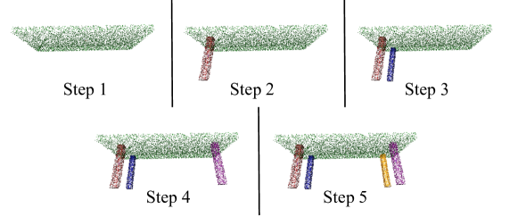
Figure 6: Visualization of the Lack [Table] assembly steps. See the supplementary material for more examples.

In Fig. 6, we provide snapshots from an assembly. In the video provided as supplementary material, we provide more examples, including also failure cases.

VI Conclusion

In this paper, we studied whether furniture assembly can be learned only using weak supervision, namely the 3D model of the assembled product. To this end, we proposed a novel reward function consisting of an incorrectness and an incompleteness measure that are calculated by matching the point cloud of the current assembly with the target model. We showed that our novel reward function is able to train a graph convolutional network to assemble various furniture.

Despite the promising results, our work can be extended in many ways. First of all, our reward function may fail to capture attachment of small parts or isotropic parts, and it can be improved by designing better incorrectness and incompleteness measures. Moreover, instead of using connection sites to assemble parts, the action space of the policy can be changed for the agent to estimate geometric relations between the parts. Lastly, a robotic controller can be used for part manipulation to incorporate robot arm constraints while learning to assemble furniture.

References

- [1] M. Yu, L. Shao, Z. Chen, T. Wu, Q. Fan, K. Mo, and H. Dong, “Roboassembly: Learning generalizable furniture assembly policy in a novel multi-robot contact-rich simulation environment,” ArXiv: 2112.10143, 2021.
- [2] N. Funk, G. Chalvatzaki, B. Belousov, and J. Peters, “Learn2assemble with structured representations and search for robotic architectural construction,” in CoRL, 2021.
- [3] Y. Lee, E. S. Hu, and J. J. Lim, “IKEA furniture assembly environment for long-horizon complex manipulation tasks,” in ICRA, 2021.
- [4] P. Jiménez, “Survey on assembly sequencing: a combinatorial and geometrical perspective,” J. Intel. Manufacturing, vol. 24, no. 2, 2013.
- [5] T. A. Abdullah, K. Popplewell, and C. J. Page, “A review of the support tools for the process of assembly method selection and assembly planning,” IJPR, vol. 41, no. 11, pp. 2391–2410, 2003.
- [6] L. Homem de Mello and A. Sanderson, “And/or graph representation of assembly plans,” IEEE T. RA, vol. 6, no. 2, pp. 188–199, 1990.
- [7] A. N. Harish, R. Nagar, and S. Raman, “Rgl-net: A recurrent graph learning framework for progressive part assembly,” WACV, 2022.
- [8] M. V. A. R. Bahubalendruni, B. Biswal, and G. Khanolkar, “A review on graphical assembly sequence representation methods and their advancements,” J. of Mechatronics and Automation, vol. 1, 2015.
- [9] L. Kavraki, J.-C. Latombe, and R. H. Wilson, “On the complexity of assembly partitioning,” Inf. Proces. Letters, vol. 48, no. 5, 1993.
- [10] Y. Huang and C. G. Lee, “A framework of knowledge-based assembly planning,” in ICRA, 1991.
- [11] S. Lee, “Backward assembly planning with assembly cost analysis,” in ICRA, 1992.
- [12] S. Ghandi and E. Masehian, “Review and taxonomies of assembly and disassembly path planning problems and approaches,” Computer-Aided Design, vol. 67, pp. 58–86, 2015.
- [13] M. Rizwan, V. Patoglu, and E. Erdem, “Human robot collaborative assembly planning: An answer set programming approach,” Theory and Practice of Logic Programming, vol. 20, no. 6, 2020.
- [14] T. Zhang and H. Mo, “Reinforcement learning for robot research: A comprehensive review and open issues,” IJARS, vol. 18, no. 3, 2021.
- [15] Y. Zhu, J. Wong, A. Mandlekar, and R. Martín-Martín, “robosuite: A modular simulation framework and benchmark for robot learning,” in arXiv preprint arXiv:2009.12293, 2020.
- [16] Y. Li, K. Mo, L. Shao, M. Sung, and L. Guibas, “Learning 3d part assembly from a single image,” arXiv 2003.09754, 2020.
- [17] J. Huang, G. Zhan, Q. Fan, K. Mo, L. Shao, B. Chen, L. Guibas, and H. Dong, “Generative 3d part assembly via dynamic graph learning,” NeurIPS, 2020.
- [18] J. Schulman, F. Wolski, P. Dhariwal, A. Radford, and O. Klimov, “Proximal policy optimization algorithms,” arXiv: 1707.06347, 2017.
- [19] C. R. Qi, L. Yi, H. Su, and L. J. Guibas, “PointNet++: Deep hierarchical feature learning on point sets in a metric space,” NeurIPS, 2017.
- [20] Z. Wu, S. Song, A. Khosla, F. Yu, L. Zhang, X. Tang, and J. Xiao, “3d shapenets: A deep representation for volumetric shapes,” in CVPR, 2015.
- [21] T. N. Kipf and M. Welling, “Semi-supervised classification with graph convolutional networks,” in ICLR, 2017.
- [22] P. Besl and N. D. McKay, “A method for registration of 3-d shapes,” PAMI, vol. 14, no. 2, pp. 239–256, 1992.
- [23] G. Brockman, V. Cheung, L. Pettersson, J. Schneider, J. Schulman, J. Tang, and W. Zaremba, “Openai gym,” 2016.
- [24] A. Raffin, “Rl baselines3 zoo,” https://github.com/DLR-RM/rl-baselines3-zoo, 2020.