Progress on the simulation tools for the SOXS spectrograph: Exposure time calculator and End-to-End simulator

Abstract

We present the progresses of the simulation tools, the Exposure Time Calculator (ETC) and End-to-End simulator (E2E), for the Son Of X-Shooter (SOXS) instrument at the ESO-NTT 3.58-meter telescope. The SOXS will be a single object spectroscopic facility, made by a two-arms high-efficiency spectrograph, able to cover the spectral range 350-2000 nanometer with a mean resolving power R$\approx$4500. While the purpose of the ETC is the estimate, to the best possible accuracy, of the Signal-to-Noise ratio (SNR), the E2E model allows us to simulate the propagation of photons, starting from the scientific target of interest, up to the detectors. We detail the ETC and E2E architectures, computational models and functionalities. The interface of the E2E with external simulation modules and with the pipeline are described, too. Synthetic spectral formats, related to different seeing and observing conditions, and calibration frames to be ingested by the pipeline are also presented.

1 INTRODUCTION

Exposure Time Calculators (ETC) and End-to-End simulators (E2E) are valuable tools that can provide multiple functionalities at different stages of the instrument building. The purpose of ETCs is to provide the team and scientists with a fast, reliable, and easy-to-use tool that can produce valuable information about the instrument in relation to a specific astronomical observation, the signal-to-noise ratio (SNR) is an example. End-to-End instrument models (E2E) are numerical simulators, which aim at simulating the expected astronomical observations starting from the radiation of the scientific sources (or calibration sources in the case of calibration frames) to the raw-frame data produced by instruments. Synthetic raw-frames can be ingested by the Data Reduction Software (DRS) to be analyzed in order to assess if top-level scientific requirements (such as spectral resolution, SNR) related to the specific science drivers, are satisfied with the specific instrument design. E2Es have been valuable software exploited in many types of astronomical instruments for different purposes. Specifically, they have been used in design phases to optimize and improve specific hardware components and parameters[1], or for early verification of instrument performance[2]. From the scientific point of view, they have been extensively exploited for assessing the feasibility of particularly challenging observations[3]. Furthermore, instrument simulators are systematically exploited to aid both Data Reduction[4] and Data Analysis Software development, as well as for testing and verifying of existing data reduction pipelines. In fact, in the specific case of SOXS, the E2E simulator, which will be here presented, has a key goal to drive the optimization of the DRS development. In addition, it will also be a reliable tool to help the setting of calibration procedures and observation plans.

This paper is organized as follows, in Section 2, an overview of the SOXS instrument is given. The Simulator, along with its architecture, simulated frames and iteration with Data Reduction Software is discussed in Section 3 and the Exposure Time Calculator is described in Section 4.

2 The SOXS Instrument

SOXS is a wide-band spectrograph for the ESO-NTT in La Silla (it will be installed at one of the Nasmyth foci of the NTT) covering in a single exposure the spectral range from the UV to the NIR (350-2000 nanometer). Its central structure (the common path) supports two distinct spectrographs, one operating in the UV-VIS 350-850 nanometer and the other in the NIR 800-2000 nanometer wavelength ranges, respectively. Both spectrographs can operate independently at different resolutions according to the slit widths: R$\approx$10000 with $0.5"$ slit, R$\approx$4500 with $1"$ slit and R$\approx$3300 with $1.5"$ slit. See general overview here [5, 6].

The two arms are fed by the light coming through a common opto-mechanical system (the Common Path [7]). It redirects the light from the telescope focus to the spectrograph slits through relay optics reducing the F/number (from F/11 to F/6) and compensating for the atmospheric dispersion (only in the UV-VIS). The Common Path provides also the mechanism to drive the light to/from the other instrument subsystems, i.e. the acquisition camera and the calibration unit.

The Acquisition Camera subsystem has different functions: acquisition of the target for the spectrographs, monitoring of spectrographs co‐alignment and light imaging. It consists of a moving stage with positions enabling the various functions, a folding mirror, a filter wheel (u, g, r, i, z, y LSST and V Johnson bands) front of a compact camera which relays the Nasmyth focus (field of view of $3.5\times 3.5$ arcmin) on the 13.0 $\mu$m, $1024\times 1024$ pixel detector CCD. See for details [8].

The UV-VIS spectrograph arm is based on a novel multi-grating concept (for details[9] and Fig. 1), in which the incoming beam is partitioned into four polychromatic beams using dichroic surfaces, each covering a waveband range of $\sim 100$ nanometer, named as quasi-order. Each quasi-order is diffracted by an ion-etched grating. The detector, located 4 mm behind the camera field flattener back surface, is an e2V CCD44-82 CCD ($2048\times 4096$ pixels, pixel size 15 micrometer, see for details[10]). The near infrared spectrograph, showed in Fig. 2, is a cross-dispersed echelle, with R$\sim 5000$ (for $1^{\prime\prime}$ slit), covering the wavelength range from 800 to 2000 nanometer with 15 orders (see for details[11]). It is based on the 4C concept, characterized by a very compact layout, reduced weight of optics and mechanics, and good stiffness. The spectrograph is composed of a double-pass collimator and a refractive camera, an R-1 grating as main disperser and a prism-based cross disperser. The detector is a Teledyne H2RG array operated at 40K, $2048\times 2048$ pixels, pixel size 18 micrometer (see for details[12]).

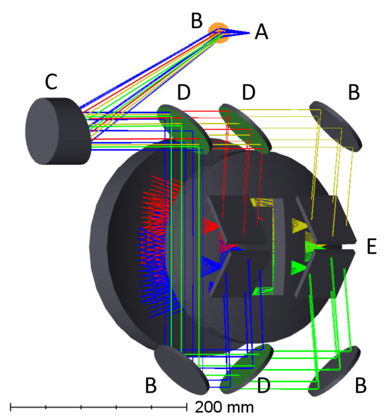
Figure 1: SOXS UV-VIS spectrograph complete optical layout. A. slit plane, B. reflective mirrors, C. OAP Collimator, D. dichroic filters, E. gratings.

Figure 2: SOXS NIR spectrograph complete optical layout. The optical beams goes the double pass collimating and cross-dispersing optics. The main disperser is a $44\deg$ blaze angle echelle grating. A field mirror redirect the beam down to the camera.

The calibration unit, provides the calibration spectra to remove the instrument signature. The calibration spectra are generated using a synthetic light source, adopting an integrating sphere equipped with lamps suitable for wavelength and flux calibrations across the full wavelength range of the instrument (350-2000 nanometer); for details see[13]. The following lamps are used:

• Quartz-tungsten-halogen (QTH) lamp, for flat field frames 500-2000 nanometer;

• Deuterium (D2) lamp, for flat field 350-500 nanometer (used simultaneously with QTH lamp for UV-VIS arm);

• ThAr hollow cathode lamp, for UV-VIS wavelength calibration;

• Ne-Ar-Hg-Xe pen-ray lamps bundled together, for NIR wavelength calibration. The individual lamps are controlled to operate together as one lamp.

The instrument is now under intense AIT phase in the consortium premises (Astronomical Observatories of Padova and Merate, Italy) as detailed in several contributions [6, 14, 15, 16].

3 End-to-End simulator

The End-to-End simulator architecture is highly modular, composed by different modules (each one with specific tasks and functionalities) units and interfaces, as described in the schematic workflow of Fig. 3. Modularity and flexibility are key points in the definition of tasks and interfaces among different modules or units to allow this tool for being scalable and adaptable to different kind of simulations (science versus calibrations frames) and spectroscopic instrumentation. The simulator is written in Python 3.9 and uses specific libraries for specific functionalities and for interfacing with other software, like commercial optical ray tracing Zemax-OpticStudio®.

Figure 3: E2E simulator workflow schematic description. The solid arrows represent the real light path, while the dashed arrows show: the simulation data-flow, how the different modules and units are interfaced and their connection to the simulator core, which is the Image Simulation Module. Orange blocks are units of the Instrument Module, while blue blocks are related to simulation modules independent from the specific instrument.

3.1 The Simulator Architecture

In the following a brief description of the modules and units showed in the workflow diagram is given; more details can be found here [17].

3.1.1 Science Module

The Science Object Module has the purpose to generate a synthetic 1D spectrum related to a specific astronomical source, at a resolution higher than the one selected for the instrument simulation (which is related to the instrumental resolution dependent on the slit width). The 1D spectral flux density distribution is obtained by a set of parameters (e.g. object type - spectral type for stars -, magnitude and redshift) or by loading the spectrum from a user-defined library. An example of a synthetic 1D spectrum for a G0V star (Pickels model) sampled at resolution of 0.5 Angstrom , is shown in the Fig. 4.

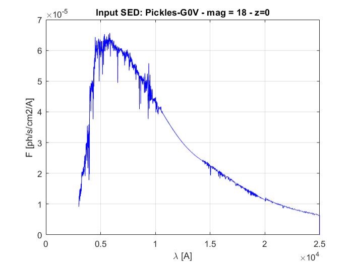
Figure 4: Example of a synthetic 1D spectrum for a G0V star (Pickels model) sampled at resolution of 0.5 Å, mag 18 (V band of Johnson-Cousins filters, in Vega magnitude system) and at $z=0$.

3.1.2 Sky-Atmosphere Module

The task of this module is to model the scattering, absorption and emission occurring in the Earth’s atmosphere. This is done by calling sky-emission and atmospheric transmission spectra of a dedicated library built using the ESO SkyCalc tool (available at the web page[18]). The sky radiance spectrum loaded is in units of photon second meter² micrometer arcsec², thus it is first calculated for the on-sky area related to the slit length and selected slit width according to the simulation (both in arcsec ) and then the units are converted in photon second cm² Angstrom ).

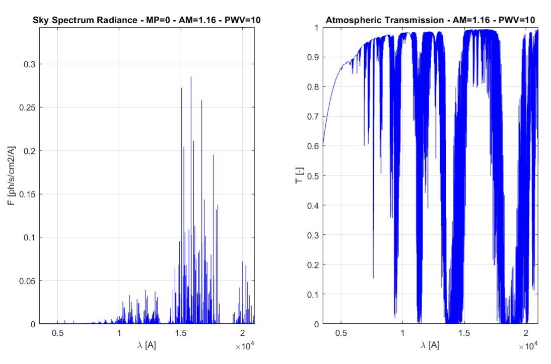
Figure 5: Example of a sky radiance spectrum and atmospheric transmission calculated through the ESO-SkyCalc tool. New moon, air-mass=1.16 and precipitable water vapor (PWV) = 10 mm

3.1.3 Telescope Module

The aim of this module is to predict the telescope throughput based on the available telescope mirrors reflectivity data. For the NTT a global telescope throughput of 0.61 is considered, given the three reflections along the telescope optical path.

3.1.4 Calibration Unit

The calibration unit is in charge of simulating the Spectral Energy Distribution (SED) of the calibration sources. This unit requires to know which kind of lamps are to be simulated flats lamp or ThAr and pen-rays lamps, according to the specific calibration frame to be generated, the instrument resolution and the type of calibration mask. In fact, SOXS foresees a single pinhole and a multi pinholes (9 pinholes) mask for calibrations and DRS purposes. Examples of the QTH spectrum (in UV-VIS) and penrays (Ar-Hg-Ne-Xe) spectrum in the NIR are shown in Fig. 6.

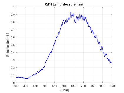
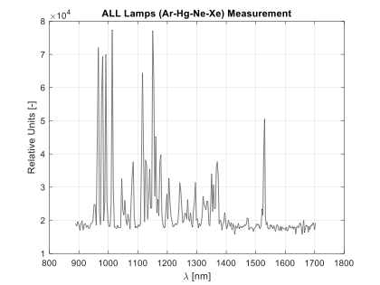
Figure 6: Example of calibration sources spectra used in SOXS. Left panel: QTH spectrum, right panel: penrays. Both spectra have been measured by the Calibration Unit work-package team.

3.1.5 Common Path Unit and Slit Unit

The task of the Common-Path (CP) unit is to predict the light distribution at the CP focal plane and throughput for both the UV-VIS arm and NIR arm. The required inputs are seeing value for the observing conditions, the CP image scale and the optics data regarding glasses, coatings and mirrors reflectivity, in order to estimate the image on the CP focal plane and the efficiency.

Figure 7: Left panel: common-Path UV-VIS arm efficiency, in black bold line, while in colored lines the single Common-Path optical elements efficiency. Dich – Dichroic, FM – folding mirror, ADC – atmospheric dispersion corrector, TT – tip-tilt mirror, FL – field lens. Right panel: common-Path NIR arm efficiency, in black bold line, while in colored lines the single Common-Path optical elements efficiency. Dich – Dichroic, FM – folding mirror, TT – tip-tilt mirror, L01 – lens 1 (refocuser), WIN – window, L02 – lens2 (field lens).

The slit-unit calculates the fraction of light passing through the UV-VIS and NIR slits, which are located on their respective common-path arms focal plane, from the variation of seeing in wavelength (w.r.t. the reference value set at 5000 Angstrom ), airmass, atmospheric turbulence parameters and considering the specific sizes (the slit length is constant $12"$, while the width changes according to the simulated set of instrument parameters).

3.1.6 Spectrograph Unit

The purpose of this unit is to simulate the physical effects of the different optical components of the spectrometers with the final aim of predict the echellogram (spectral format) at the UV-VIS and NIR focal plane, the throughput and a database of Point Spread Function (PSF) maps for a set spectral resolution element (which are used by the Image Simulation Module for rendering the synthetic frames).
The UV-VIS quasi-orders and NIR orders efficiency (from spectrograph entrance to focal plane, detector QE excluded) are shown in Fig. 8.

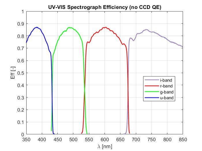
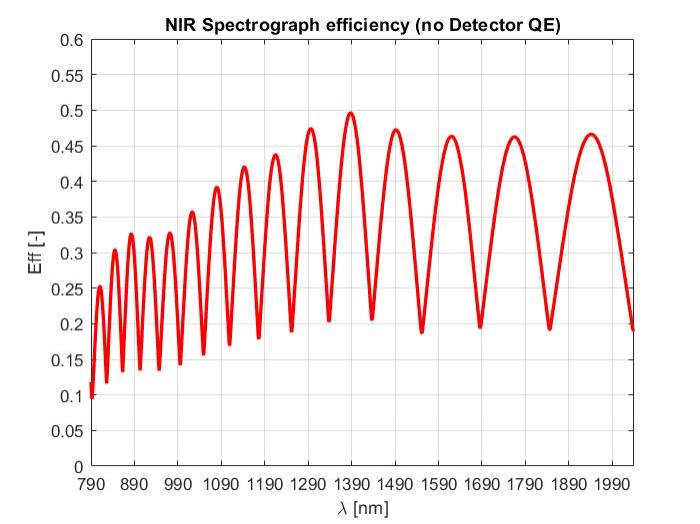
Figure 8: Spectrograph efficiency profiles (detector QE excluded) Left panel: UV-VIS spectrograph quasi orders. Right panel: NIR.

The PSF maps database is computed by directly querying the optical design ray-tracing files (built with commercial optical design software Zemax-OpticStudio®), using specific API-based software codes to extract the required data for a defined set of wavelengths along each diffraction order (or the for quasi-orders in the UV-VIS arm). In particular, the PSF maps are calculated using the Huygens PSF analysis tool of Zemax-OpticStudio®, which includes diffraction and optical aberrations. Being SOXS a long slit spectrograph, the PSF map for each database wavelength can be computed both from an average of the PSF maps, 64micrometer wide, related to five positions along the slit (-0.662, -0.331, 0, 0.331, 0.662 mm , corresponding to -6, -3, 0, 3, 6 arcsec ), and by interpolating along slit direction the map of these five positions, according to the required simulation. Examples for both arms, first UV-VIS then NIR, in Fig. 9.

(a)

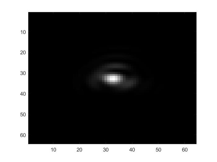
(b)

Figure 9: Example of PSF maps, 64 micrometer wide, computed for center slit position. Left panel: UV-VIS spectrograph. Right Panel: NIR spectrograph.

The spectral format data, required to produce the synthetic echellograms by the Image Simulation Module, are the diffraction order number (or quasi order id, for UV-VIS), wavelength (the same set used in the computation of the PSF maps database), centroid coordinates of both the central slit position and edges (through which the slit image tilt on the focal plane is computed) and slit image size (i.e. the geometrical full width in main dispersion and spatial direction).

The full database, comprised of efficiency, PSF maps and spectral format, produced by the Spectrograph Unit is stored for the usage of the Image Simulation Module.

3.1.7 Image Simulation Module

This portion of the simulator is the kernel of the whole system and put together the outputs of all the other modules and units. This piece of software is responsible for rendering the photons distribution of each spectral resolution element for each order as should be detected at the level of spectrographs focal plane by the detectors. In particular, the module first interpolates on a sub-pixel scale, of which the oversampling can be set according to the required simulation accuracy, all the instrumental data regarding wavelength, image centroid coordinates, sampling (in both main dispersion and spatial directions), slit image tilt, average PSF map and efficiency. Then, it produces the photons distribution of each wavelength in sub-pixel scale by convolving the slit (long slit or pinhole masks according to the specific science or calibration frame type) image with the corresponding PSF map. The spectral slit images are properly sized and tilted according to the sampling and tilt variation along each order, and scaled for the integrated spectral flux and efficiency. The code architecture has been developed in order to properly exploit the functionality of numba[19] and to take advantage of the parallel features of the concurrent Python package, such that the different diffraction orders (or a fraction of them) can run in parallel. Once all the spectral images have been piled up to sum their photons distribution at sub-pixel scale, the synthetic frame is re-binned to pixel scale. Then, the photon noise and all other specific detector noises are added by the Detector Module.

3.1.8 Detector Module

The detector module exploits the Pyxel [20] simulation framework to model the different detector effects on the rendered data at pixel scale. This tool works through a series of modules that are executed in cascade simulating the whole detection chain. For example, at the photon generation level, it is possible to model the shot noise, while the quantum efficiency (QE), dark current (DC), and the effect of cosmic ray are added at the charge generation level. Several other effects can be added at different levels of the simulation, including read-out noise (RON), bias levels, fix pattern noise caused by pixels non-uniform response (PRNU), pixel cross-talk (due to charge diffusion) and more. In addition, for NIR detectors a specific module, the HxRG noise generator, allows to model the kTC bias noise, white readout noise and alternating column noise (ACN). Through this framework, it is also possible to generate bias and dark frames for calibrations. The QE curves for both the UV-VIS CCD and the NIR detector implemented in the simulation are shown in Fig. 10.

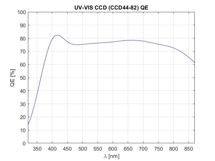
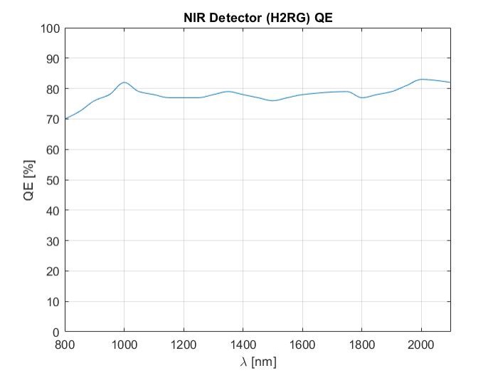
Figure 10: Spectrograph detectors QE. Left panel: UV-VIS CCD. Right panel NIR H2RG detector.

The parameters for some relevant implemented effects (extrapolated from datasheet, measurements by manufacturer tests or from same detector type in similar instrument) are the followings:

	Gain (ADU/e-)	RON (rms e-)	DC (e/pix/s)	PNUR (%)	Cross-talk (%)
UV-VIS CCD	1.25	2.3	$2.7\times 10^{-5}$	1.6	1
NIR Detector	0.5	11 (CDS reading)	$<10^{-3}$	4	0.5

3.2 Simulated Frames

In this section we present some examples of simulated frames generated with the E2E simulator. A first example (see Fig. 11) is the NIR synthetic image of a M2V (Pickles) stellar spectral type with V-mag = 18 (Vega System) observed at new moon with air-mass = 1, precipitable water vapor (PWV) = 10 mm , seeing = 1 arcsec (at 5000 Angstrom ) and with the selected slit width of 1 arcsec . The total exposure time is 900 seconds realized through a single exposure. A simple set of detector noises was added via Pyxel, such as shot noise, dark current (DC) and read out noise (RON). The different diffraction orders traces with the object centered in the slit and sky emission features are clearly visible.

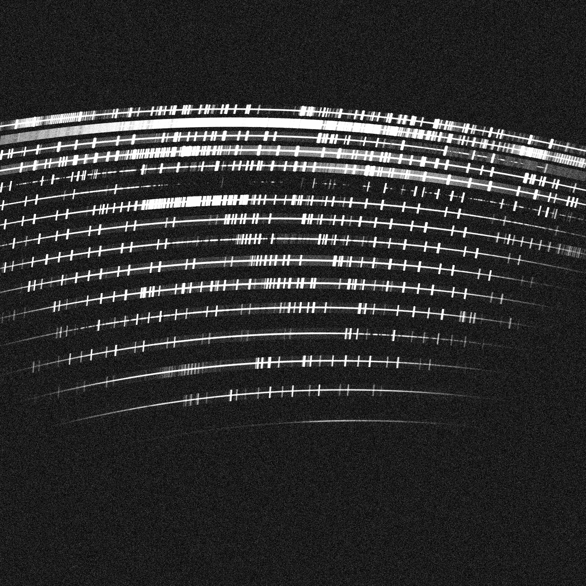
Figure 11: NIR arm synthetic science frame of a M2V (Pickles) stellar spectral type with V-mag = 18 (Vega System).

The images in Fig. 12 and Fig. 13 represent three different NIR wavelength calibration frames taken with 10 seconds of exposure that were used during the iteration with the Data Reduction Software, as discussed in the next section. In the first set of frames a flat field through the 1 arcsec slit width and a second flat field through a single pinhole are simulated. The wavelength calibration frame of Fig. 13 simulates the emission lines of the PenRays (Ar-Hg-Ne-Xe) lamps through a multi-pinhole mask. The spectral resolution elements related to the emission lines of the lamps along each order can be seen both in the full frame and in the zoomed box, where also the 9 pinholes images in cross dispersion direction can be distinguished.

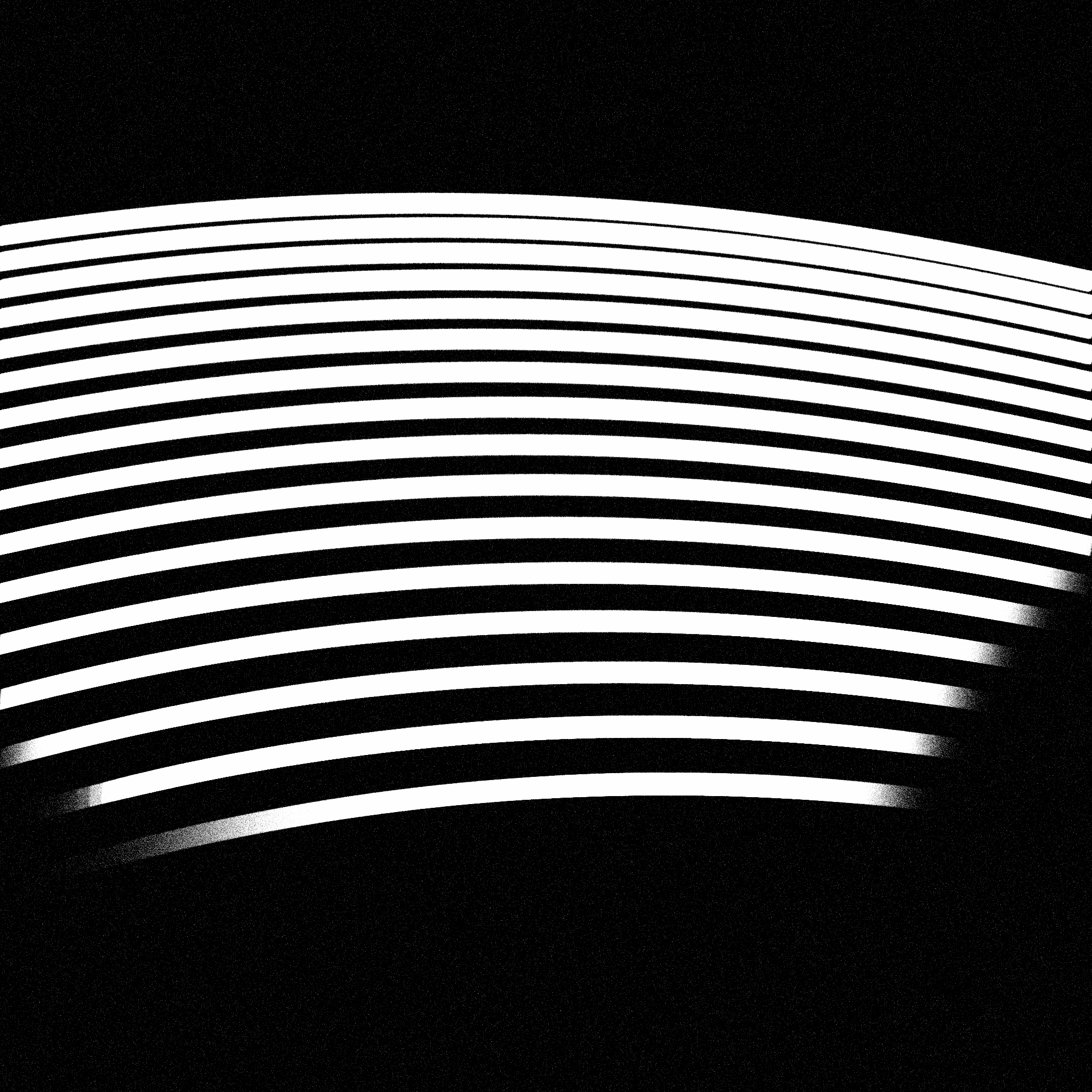
(a) Flat field through slit

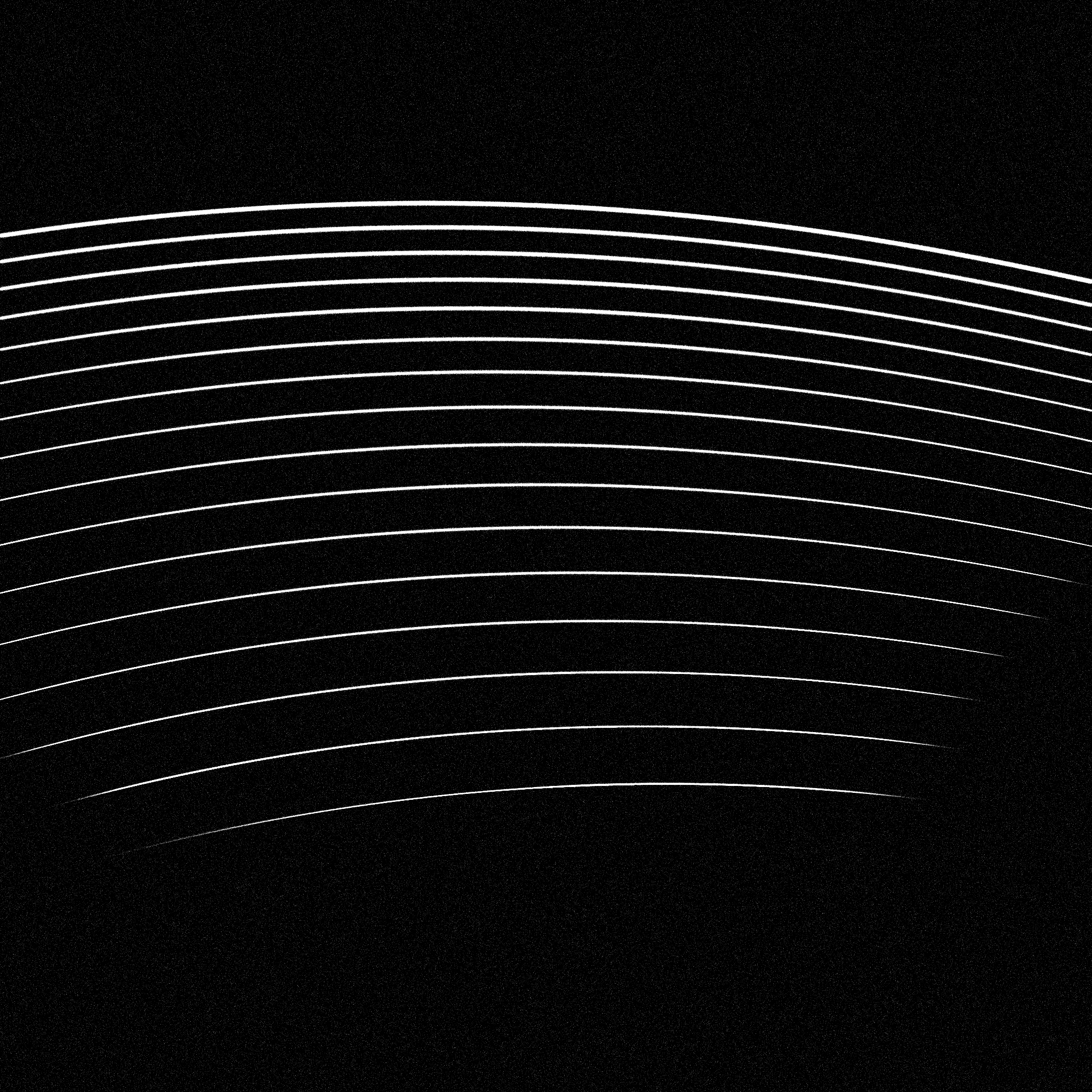
(b) Flat field through single pinhole

Figure 12: NIR arm calibration frames.

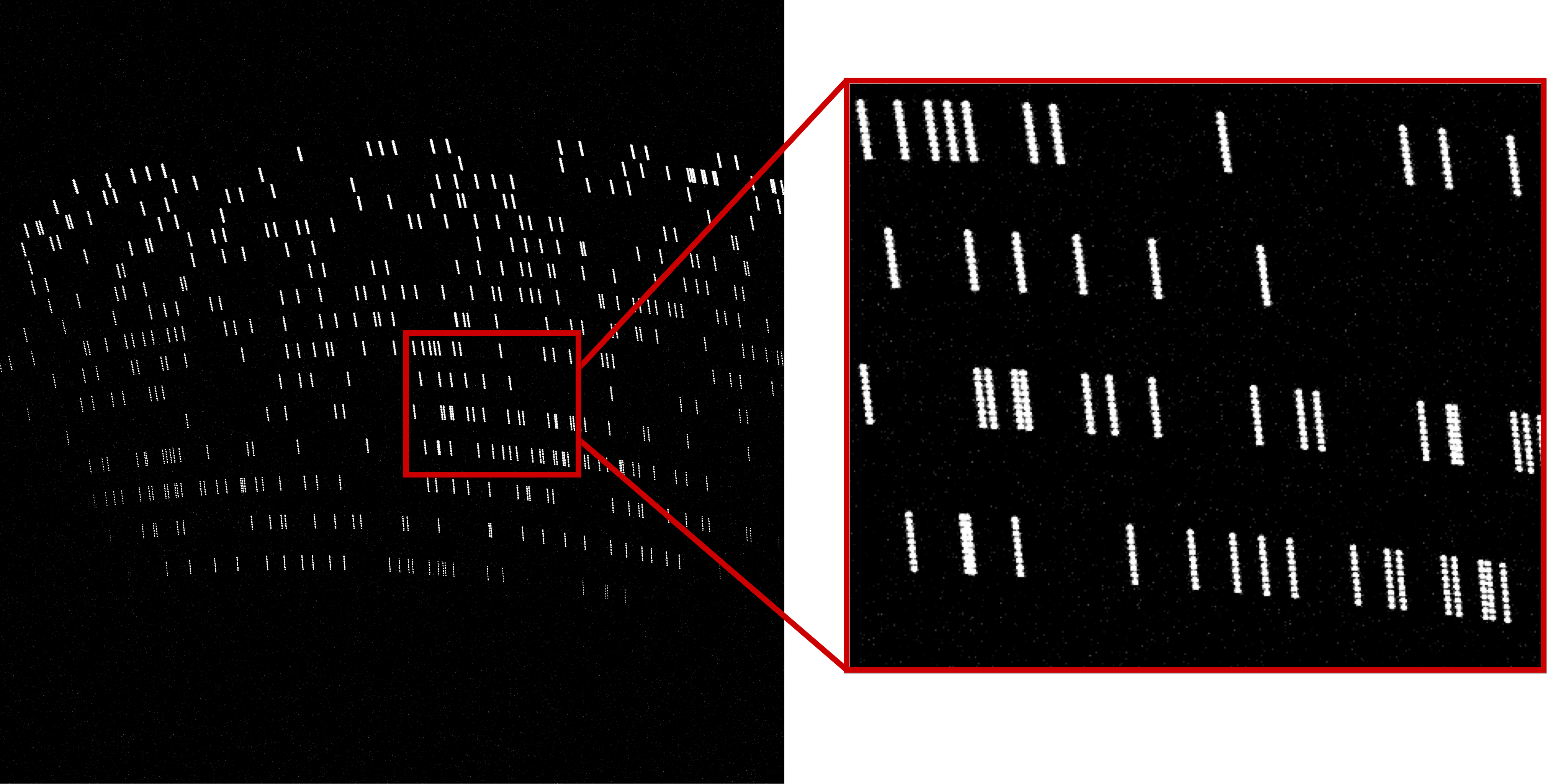
Figure 13: NIR wavelength calibration frames with PenRays (Ar-Hg-Ne-Xe) emission lines and multi-pinhole mask.

An example of how a UV-VIS science frame would looks like can be seen in Fig. 14. An observation of a G0V star, with V-mag = 18 (Vega System). The observation has been simulated again in new moon, at airmass=1.2 with sky PWV = 10 mm. The seeing assumed is 0.87 arcsec, at 550 nanometer , and the selected slit width is 1 arcsec. A single exposure of 1200 sec is emulated. The different quasi-orders traces with the object centered in the slit and sky emission features are clearly visible in the top and bottom quasi-orders, which are $r$-band and $i$-band respectively. While in the $u$-band (the second quasi-order from the top), the combined effect of star SED, instrument resolution, seeing and atmospheric transmission result in a trace that has 80% lower photon flux with respect to the $i$-band for example. The slit tilt of the different spectral resolution elements images can be visually noticed mostly in the bottom quasi-order ($i$-band) thanks to greater contrast and presence of sky emission lines. The presence of hot/bad pixels and cosmic rays, for this frame, has been uniformly simulated across detector area.

Figure 14: UV-VIS arm simulated synthetic frame of a science observation of a G0V star $V$-mag = 18 (Vega System). See text for other simulation details.

Fig. 15 shows a flat slit calibration frame in the UV-VIS, with QTH+D2 combined sources and 10 sec of exposure. The $r$-band and $g$-band (1st and 3rd from top respectively) have a sharp cut-off at the spectral range edge. The $u$-band exhibits a lower flux at the beginning of its wavelength range due to the CCD-QE (see Fig. 10, left panel), while the $i$-band is affected by the UV-VIS/NIR dichroic transition region above 800 nanometer (see Fig. 7), as can be seen from the right side of its trace (the bottom one).

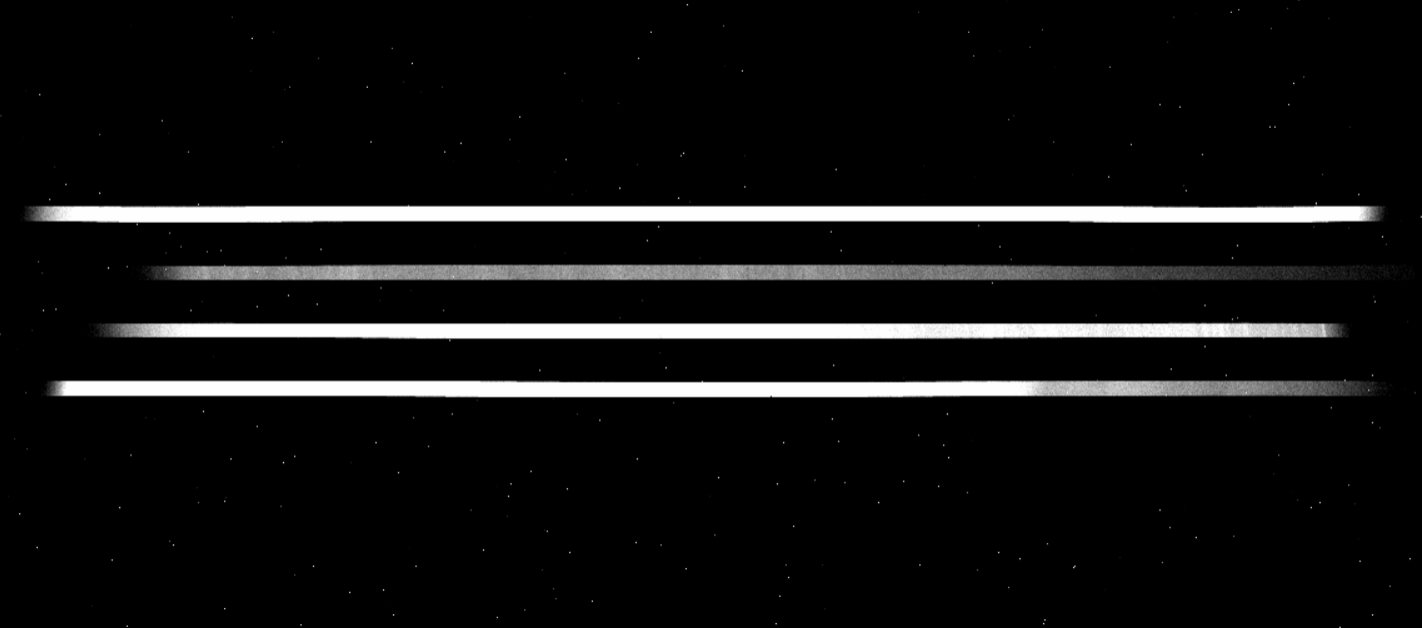
Figure 15: UV-VIS calibration frame. Flat slit with QTH+D2 lamps and 10 sec of exposure.

3.3 Data Reduction Software Iteration

It is a significant boon for the pipeline development team, and the SOXS Consortium as a whole, having simulated frames in the expected SOXS format before integration and commissioning of the instrument. Much of the pipeline development effort and debugging has already been performed ahead of time before the pipeline has been introduced to real SOXS data.

The SOXS data reduction pipeline (soxspipe, [soxs_drs022]) development team have exploited the availability of simulated NIR SOXS data frames to test and hone many of the routines used across the reduction cascade.

Fig. 16 show the results of a first-guess dispersion solution obtained by soxspipe using a simulated arc-lamp frame obscured by a single-pinhole mask. The arc lines detected in the frame (top image panel) are used to fit a global dispersion solution (second image panel). The residuals of the fit compared to the observed arc-line positions are presented in a x-y dispersion (residuals mean 0.13 pixels, standard deviation 0.07 pixels) and histogram plots in the bottom image panel. Fig. 17 reveals how soxspipe then uses this first-guess dispersion solution, alongside a simulated flat-lamp frame, again obscured by the single-pinhole mask, to determine the traces of the centre of each of the spectral orders. Locations along the order centre traces (top image panel) are used to fit a global solution to the traces (second image panel). The residuals of the fit (residuals mean 0.04 pixels, standard deviation 0.03 pixels) and a plot of the trace FWHM (along spatial direction, in units of pixels) dependence on wavelength can be found in the bottom panels. Fig. 18 shows the use of the centre trace solutions and a set of simulated NIR slit lamp-flat frames to a) create a master-flat frame and b) detect and fit the edges of each order on the frame. Measured pixel locations of the order edges (top image panel) are used to fit a global solution to the edges (second image panel). The residuals of the fit compared to the measured edge pixel locations can be found in the bottom panels (residuals mean 0.12 pixels, standard deviation 0.09 pixels). Finally, Fig. 19 shows the use of the first-guess dispersion solution, the order location solutions and a simulated arc-frame, obscured this time by a multi-pinhole mask, to determine the final full-dispersion and spatial solution required to reduce object frames later in the reduction cascade. The arc lines detected in the frame (top image panel) are used to fit a global dispersion solution (second image panel). The residuals of the fit compared to the observed arc-line positions can be found in the bottom panels as x-y dispersion (residuals mean 0.15 pixels, standard deviation 0.09 pixels) and histogram plots.

Alongside simulated SOXS data, soxspipe has the ability to reduce X-shooter data. The low residuals achieved while finding global best-fit polynomials for the order-centre traces, order-edges and dispersion solutions within simulated SOXS data, closely resemble those found reducing X-shooter data with both soxspipe and the original X-shooter data-reduction pipeline [21].

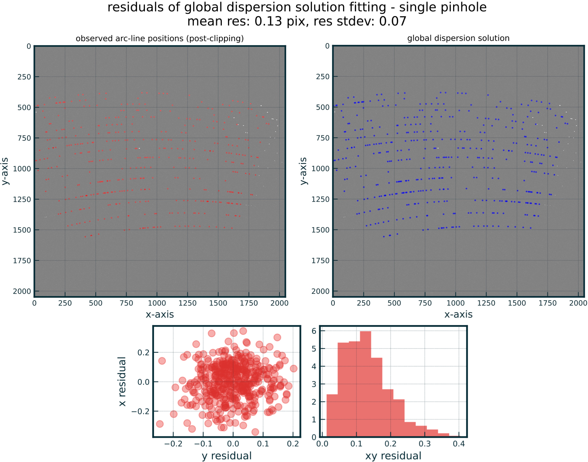
Figure 16: The resulting first-guess dispersion solution and residuals as fitted by the SOXS data-reduction pipeline using a simulated arc-lamp frame obscured by a single-pinhole mask.

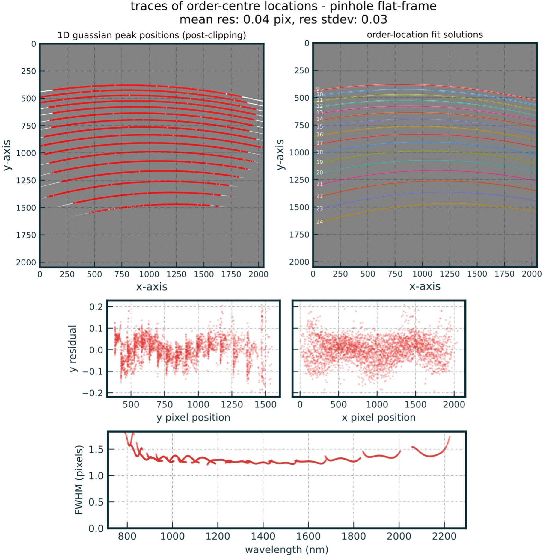
Figure 17: The order-centre traces fitted by the SOXS data-reduction pipeline using a simulated flat-lamp frame obscured by a single-pinhole mask.

Figure 18: The order-edges fitted by the SOXS data-reduction pipeline using a master-flat frame created from a set of simulated full slit flat-lamp frames.

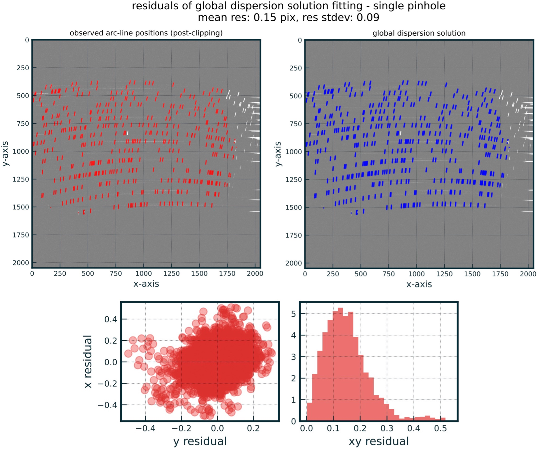
Figure 19: The resulting final dispersion solution and residuals as fitted by the SOXS data-reduction pipeline using a simulated arc-lamp frame obscured by a multi-pinhole mask.

4 Exposure Time Calculator

The Exposure Time Calculator of SOXS is a web-based tool that reflects the two different modes of observation, spectroscopy and imaging. The architecture for both modes was developed based on the structure of the previously described end-to-end simulator, sharing at a high level a similar workflow of modules and units and at lower level the required mathematical recipes. Each unit was tested individually and compared with several ETCs from ESO. The ETC was developed via Python 3.9 using the web application framework Flask (2.0). This tool has already been useful at different stages of development to evaluate the performance of the instrument (see comparison with VLT-X-shooter for Spectroscopy and with NTT-EFOSC2 for imaging in Section 4.3) and it will be widely used by scientists when SOXS will be in operations.

4.1 ETC Architecture

The workflow of the ETC starts from generating a synthetic 1D spectrum in units of photon s cm² angstrom and computing the Sky Radiance and the Atmospheric Transmission profiles (from ESO’s SkyCalc tool) as already described in Sections 3.1.1 and 3.1.2). The number of object and sky counts in terms of photo-electrons per spectral bin are then be calculated by integrating over a delta lambda (wavelength bin) per SRE or per Pixel based on user selection, multiplying by the telescope effective area and the total exposure time (according to the single exposure integration time and number of exposures, see Fig. 22). The final results, provided for both UV-VIS and NIR arms, take into account the different optical and slit efficiencies and the detector noises.

4.2 Layout

The design of the web application was developed to be intuitive and easy to use; once the spectroscopy or imaging mode is initially selected via a toggle, the user has to fill in the several parameters, relevant for the observations, through a public HTML interface via the SOXS website as described in the following. The 1D synthetic spectrum can be obtained from four different selection’s of SEDs:

• Black Body;

• Power-Law;

• User-defined Spectrum (Possibility of selecting a pre-loaded spectrum);

• Single Emission Line.

The user must also select the magnitude of the object with its reference band and system, the redshift and if the spatial distribution is point-like or from an extended source, as shown in Fig. 20. The different parameters box are in light grey or dark grey according to the type of selected SED. For example, if power law is selected, only the power-law index and magnitude parameters can be set, while the others cannot be modified. Subsequently, the call to ESO’s SkyCalc tool will be made by setting the following inputs (see box in in Fig. 21):

• Days from new moon;

• Airmass;

• Precipitable Water Vapor (PWV);

• Seeing (reference value at zenith and 500 nanometer ).

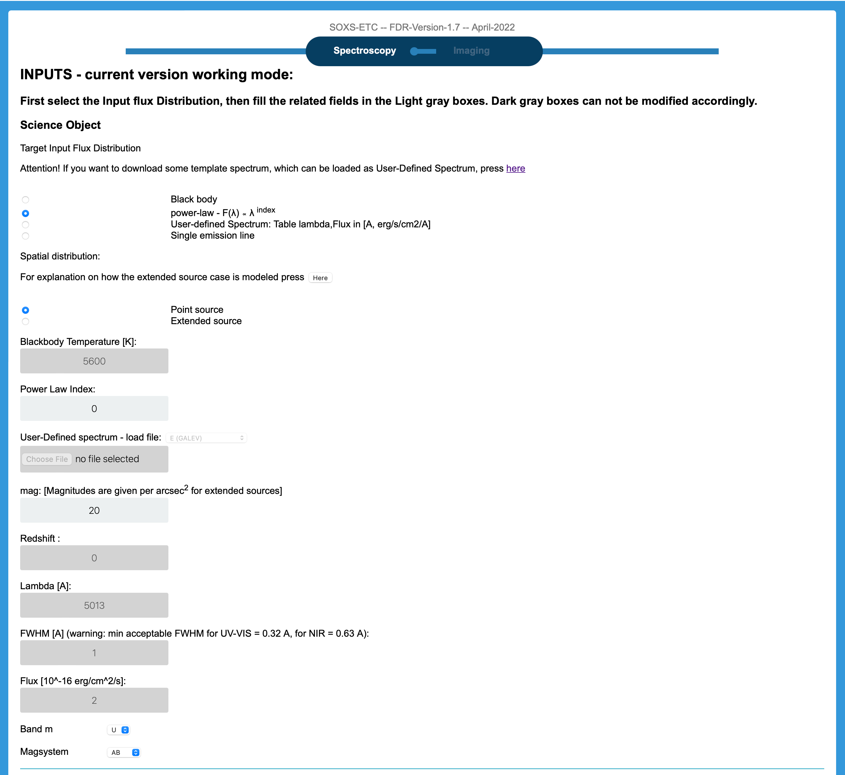
Figure 20: Graphical layout of the ETC simulator of SOXS. Science-Object input flux distribution.

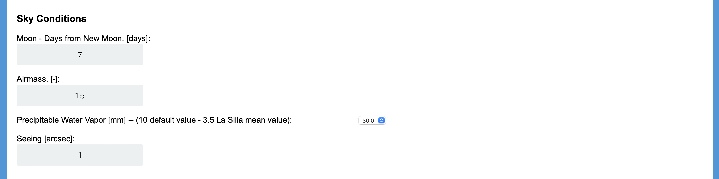
Figure 21: Graphical layout of the ETC simulator of SOXS. Sky and Atmospheric condition.

Finally, in spectroscopy mode (Fig. 22), the instrument set-up consists of the parameters of exposure time and slit size, that can be selected independently between the two arms. In addition, different number of Spectral Resolution Element per order and binning modes (only for the UV-VIS arm detector) can be selected.

While for imaging mode, a filter (among the following: u, g, r, i, z, y (LSST) and $V$ Johnson bands) and the total exposure time (exposure time for single exposure and number of exposures) parameters can be selected.

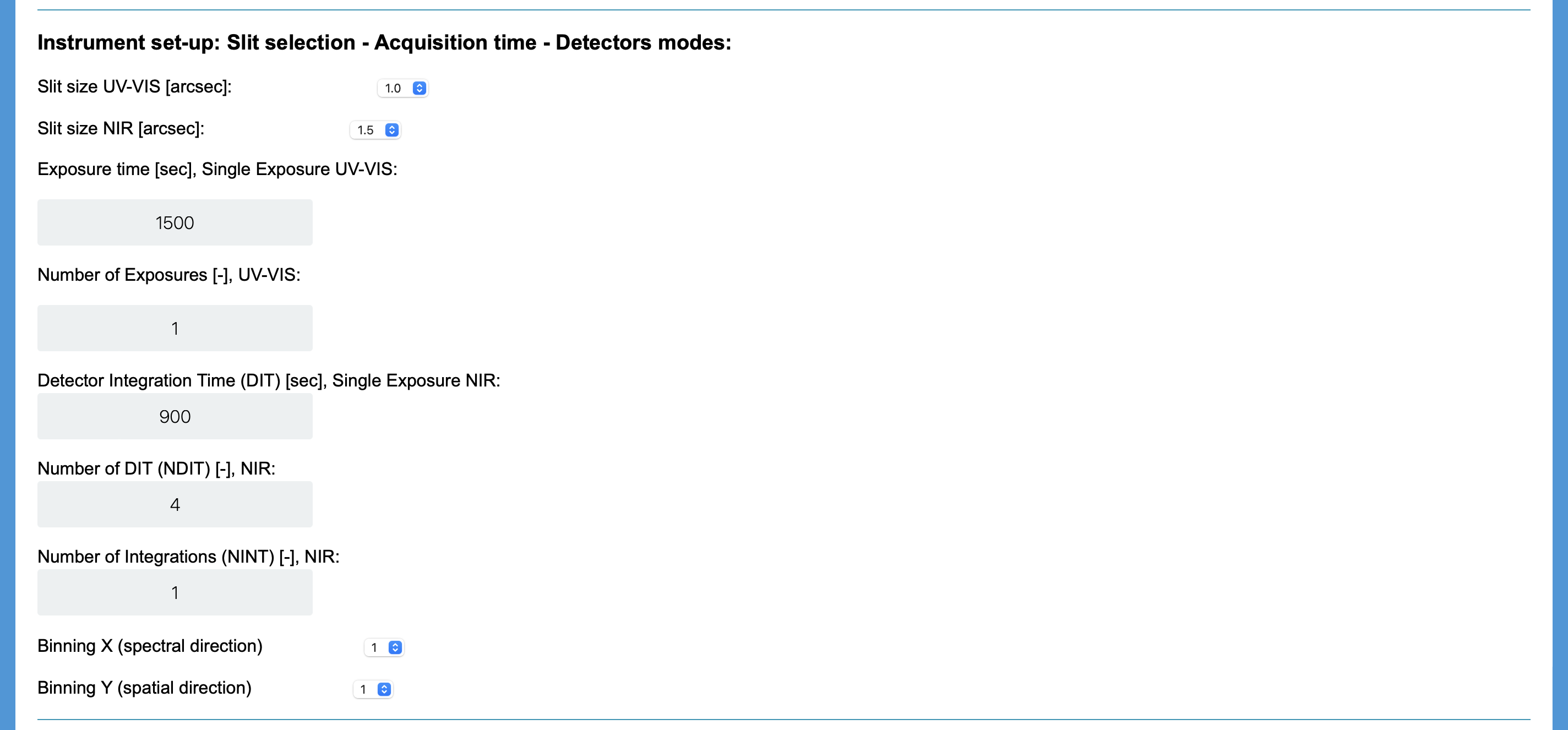
Figure 22: Graphical layout of the ETC simulator of SOXS. Instrument set-up input parameters.

4.3 Output Results

The ETC provides different outputs as listed below and in the case of spectroscopy, the same kind of information will be provided for both the UV-VIS and NIR arms.

• SNR (Spectroscopy & Imaging);

• Total efficiency (Spectroscopy & Imaging) and Filter efficiency (Imaging);

• Source Spectrum (Spectroscopy & Imaging);

• Sky radiance Spectrum & Atmospheric Transmission (Spectroscopy & Imaging);

• Source & Sky Photoelectrons (Spectroscopy & Imaging);

• Noises (Spectroscopy & Imaging);

• Maximum Intensity (Spectroscopy).

In the following example, a comparison of the output SNR between SOXS and X-shooter is presented, using both ETCs (see Fig. 23 and Fig. 24). This is done simulating a 5600 K Black Body with $R$-mag = 21.5 (AB System) observed with 4 exposures for 900 seconds and the following sky-condition: Moon phase = 0 (i.e. new moon), air-mass = 1.2, precipitable water vapor (PWV) = 30 mm and seeing = $1"$ (at 5000 Angstrom ). In the X-shooter-VIS band SOXS has a higher SNR because in this range, although the NTT telescope effective area is more than four times smaller than the VLT one, its peak instrumental efficiency is about 30% higher than X-shooter and its dispersion is such that the wavelength coverage per pixel is approximately four times larger. In the X-shooter-UVB band, SOXS has a similar instrumental efficiency but dispersion in this region is not balancing the larger effective area of the VLT. In the NIR arm, being SOXS extremely similar to X-shooter, the better performance of the latter is due to the advantages of a larger effective telescope area and telescope throughput.

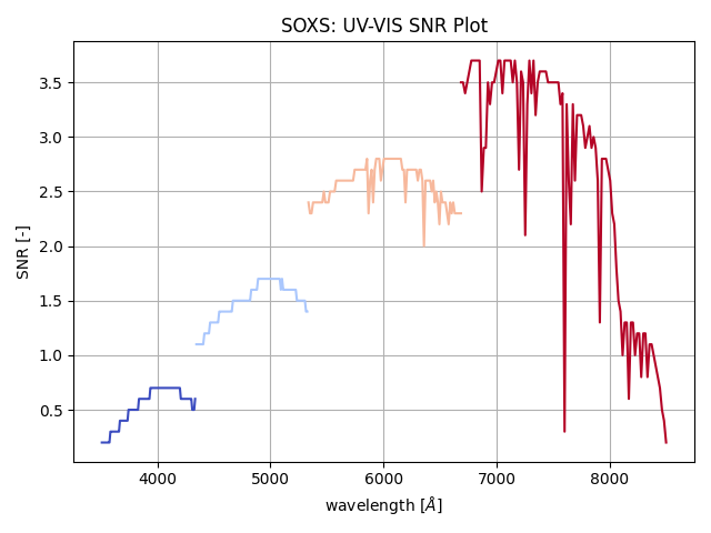
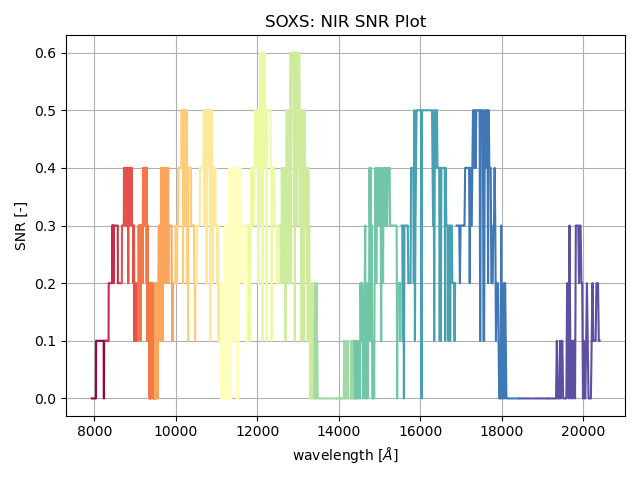
Figure 23: Black Body: 5600 K with magnitude of 21.5 (AB) $R$-Band observed with 4 exposures for 900 seconds.

(a) UVB

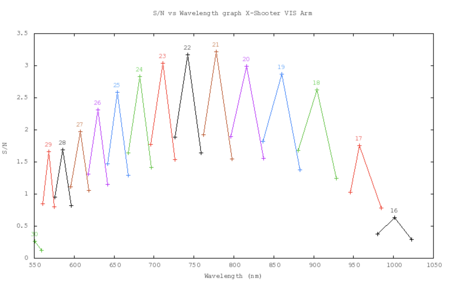
(b) VIS

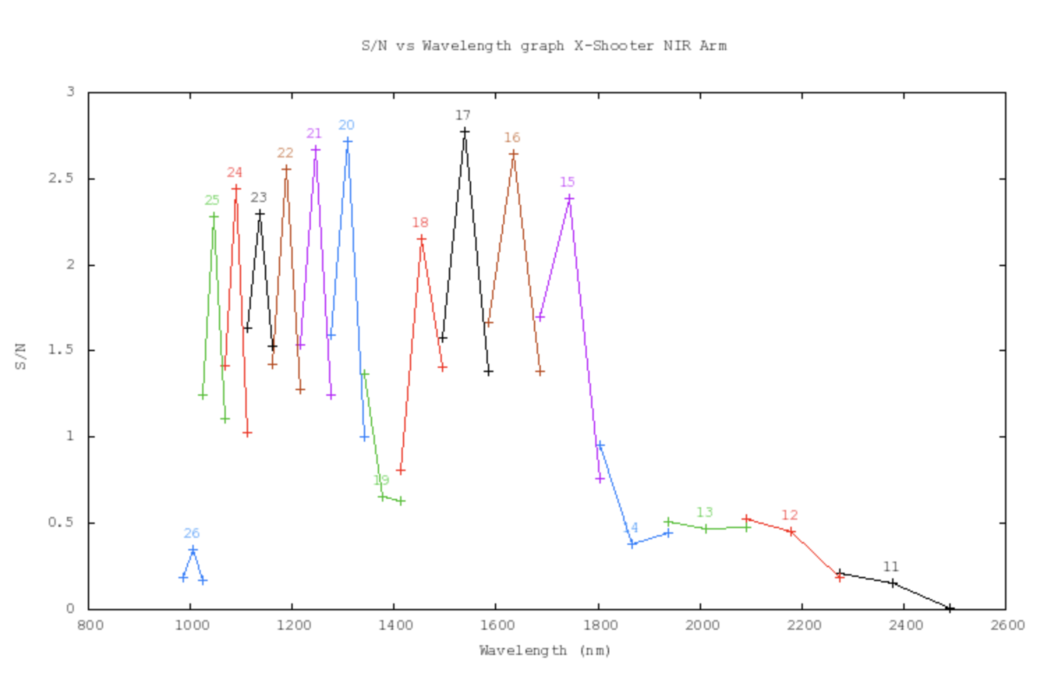
(c) NIR

Figure 24: Black Body: 5600 K with magnitude of 21.5 (AB) $R$-Band observed with 4 exposures of 900 seconds.

Regarding the imaging output, the following results were compared with the EFOSC2 instrument and can be found in Table 1; showing that by simulating a Black Body we obtain for the blue-red filters (V, g, r) a slightly worse outcome, while for the reddest filters (i, z) the performance is better.

Table 1: Performances of the ACQ Camera of SOXS comparable to EFOSC2 simulating a

SNR	SOXS	EFOSC2
$V$	7.7	10
$g$	9.4	9.8
$r$	10.18	10
$i$	7.3	6.1
$z$	4.3	3.1

5 Conclusion

In this contribution we first described the architecture and development of the NTT-SOXS E2E instrument simulator, showing both the different modules tasks and functionalities and how the Image simulation Module produce a synthetic image for both the instrument arms. Examples of simulations regarding different frames and the results obtained from iterating with the DRS for the NIR arm have been presented. This cross-check has also been fundamental to debug the simulator and to validate a full end-to-end simulation. A specific set of calibration will also be generated and used to aid the UV-VIS arm. Finally, we described the Exposure Time Calculator along with its architecture, layout and multiple outputs, for both spectroscopy and imaging observation modes.

References

- [1] Li Causi, G. et al., “Virtual MOONS: a focal plane simulator for the MOONS thousand-fiber NIR spectrograph,” Proc. of SPIE Vol. 9147, 914764 (Aug. 2014).
- [2] Bechter, A. J., Bechter, E. B., Jr., J. R. C., King, D., and Crass, J., “A radial velocity error budget for single-mode Doppler spectrographs,” Proc. of SPIE 10702, 2075 – 2099 (2018).
- [3] Bechter, E. B., Bechter, A. J., Crepp, J. R., Crass, J., and King, D., “Instrument simulator and data reduction pipeline for the iLocater spectrograph,” Publ. Astron. Soc. Pac. 131, 996 (jan 2019).
- [4] Puech, M., Yang, Y., Jégouzo, I., et al., “WEBSIM-COMPASS: a new generation scientific instrument simulator for the E-ELT,” Proc. of SPIE 9908, 2919 – 2933 (2016).
- [5] Schipani, P., Campana, S., Claudi, R., Aliverti, M., et al., “Development status of the SOXS spectrograph for the ESO-NTT telescope,” in [Ground-based and Airborne Instrumentation for Astronomy VIII ], Evans, C. J., Bryant, J. J., and Motohara, K., eds., SPIE (dec 2020).
- [6] Schipani, P. et al., “Progress on the SOXS transients chaser for the ESO-NTT,” Proc. SPIE 12184-24 (2022).
- [7] Claudi, R. et al., “The common path of SOXS (Son of X-Shooter),” Proc. SPIE 10702, 1189 – 1199 (2018).
- [8] Brucalassi, A. et al., “Final Design and development status of the Acquisition and Guiding System for SOXS,” Proc. SPIE 114475V (2020).
- [9] Rubin, A. et al., “Mits: the multi-imaging transient spectrograph for soxs,” Proc. SPIE 10702 (2018).
- [10] Cosentino, R. et al., “The vis detector system of SOXS,” Proc. SPIE 10702 (2018).
- [11] Sánchez, R. Z. et al., “Optical design of the SOXS spectrograph for ESO NTT,” Proc. SPIE 10702 (jul 2018).
- [12] Vitali, F. et al., “The NIR spectrograph for the new SOXS instrument at the NTT,” Proc. SPIE 10702, 697 – 709 (2018).
- [13] Kuncarayakti, H. et al., “Design and development of the SOXS calibration unit,” Proc. SPIE 11447 (dec 2020).
- [14] Radhakrishnan, K. et al., “From assembly to the complete integration and verification of the SOXS common path,” Proc. SPIE 12184-305 (2022).
- [15] Araiza-Durán, J. A. et al., “The integration and alignment phase for the acquisition and guiding system of SOXS,” Proc. SPIE 12184-306 (2022).
- [16] Vitali, F. et al., “Progress on the SOXS NIR spectrograph AIT,” Proc. SPIE 12184-302 (2022).
- [17] Genoni, M., Landoni, M., Causi, G. L., et al., “SOXS end-to-end simulator: development and applications for pipeline design.,” Proc. SPIE 114501B (2020).
- [18] ESO, “Skycalc,” (2013). http://www.eso.org/observing/etc/bin/gen/form?INS.MODE=swspectr+INS.NAME=SKYCALC.
- [19] Lam, S. K., Pitrou, A., and Seibert, S., “Numba: A llvm-based python jit compiler,” in [Proceedings of the Second Workshop on the LLVM Compiler Infrastructure in HPC ], LLVM ’15, Association for Computing Machinery, New York, NY, USA (2015).
- [20] Prod’homme, T., Lemmel, F., Arko, M., et al., “Pyxel: the collaborative detection simulation framework,” Proc. SPIE 1145408 (2020).
- [21] Goldoni, P., “The X-shooter pipeline,” Astronomische Nachrichten 332, 227 (Mar. 2011).