Micro-mechanical response of the F-actin/Tropomyosin/Troponin complex by optical trapping interferometry

Abstract

Single-particle optical trapping interferometry (OTI) allows us to detect the Brownian motion of a tracer bead immersed in a complex fluid with nanometric resolution and in the microsecond time-scale. By OTI, we study suspensions composed of filamentous actin (F-actin), a classic example of a semiflexible polymer, using two different kind of tracers: chemically-inert melamine resin and polystyrene depleted particles. One-particle microrheology permits to investigate the local fluctuations of the polymers in the network, but under the condition of a previous knowledge of the F-actin characteristic lengths in relation with the radius of the probes. In this work, we focus on the power-law behavior of the skeletal thin filament, composed by tropomyosin (Tm) and troponin (Tn) coupled to F-actin, which has a role in the muscle contraction by its interaction with myosin. We find that the elastic modulus for the F-actin/Tm/Tn complex in the presence of Ca²⁺ is constant until the limit of high frequencies, and that the calculated values of the power-law exponent are less dispersed than in F-actin alone, which we interpret as a micro-measurement of the filament stabilization.

I Introduction

Filamentous actin (F-actin) is an essential component in biomechanical processes, such as muscle contraction Bershitsky et al. (1997), or the mechanical properties of the cytoskeleton Bao and Suresh (2003). The thin filament, composed by tropomyosin (Tm) and troponin (Tn) coupled to actin, and regulated by the presence of calcium Ebashi et al. (1971), has a role in its interaction with myosin regarding muscle contraction. Tm is an extended molecule with length of $\sim 42\,$nm composed by a dimer of two polypeptide subunits. This molecule winds around the actin filament and is able to attach to other tropomyosin molecules into long strands, spanning the whole thin filament length Khaitlina (2015). Troponin is composed by three subunits: TnT, TnI and TnC. The subunit TnI interacts with actin, producing changes that prevent the interaction with myosin. Tm relates to TnI by facilitating the transmission of the changes on actin generated by TnI peptide along the filament Perry (2003). The calcium-regulation of the myosin-induced contraction depends on the interaction between the actin filaments, TnC and TnI Potter and Gergely (1975). Mechanically speaking, the Tm/Tn complex stabilizes the F-actin structure by increasing the stiffness of the compound Götter et al. (1996).

In this work, we investigate the modifications of the micro-mechanical behavior of F-actin by the presence of Tm/Tn through the analysis of the motion of single trapped microtracers contained in F-actin/Tm/Tn solutions. We use optical trapping interfometry (OTI) to measure, with nanometric resolution in the microsecond range Jeney et al. (2010); Franosch et al. (2011), the Brownian position fluctuations of single optically-trapped microbeads. From the motion of the tracer, it is possible to derive the microrheological properties of the surrounding medium Mason and Weitz (1995); Waigh (2005). When we use one-particle microrheology, the obtained results depend on the characteristic lengths of the network in relation with the size of the tracer bead Atakhorrami et al. (2014), i.e., this technique allows to investigate the mechanical response on the biological scales with the condition of a correct characterization of the involved length scales Schmidt et al. (2000); Buchanan et al. (2005).

In an accompanying Letter Domínguez-García et al. (2022), we have shown how the exponent values of the power-law behavior observed by OTI in the motion of single-tracer beads contained in physiological F-actin solutions depend of the combined relation between the fluid’s lengths scales, the tracers radius, their surface chemistry, and the applied optical force. In this manuscript, we detail the observations related to the F-actin/Tm/Tn complex, always in the presence of calcium, framing the literature results which clarify some assumptions made in these investigations, and we provide complete information on the calculated power-law exponents for the measured F-actin solutions, including a detailed description of the employed experimental setup and methodology.

II Experimental set-up and materials

II.1 Optical trapping interferometry

The optical trapping interferometry (OTI) system is based on a Nd:YAG laser, with a wavelength of $1064\,$nm and maximum power of $2\,$W (MEPHISTO Innolight, GmbH). The optical trap is composed of a 10x beam expander and a 60x water immersion objective (Olympus UPlanApo/IR, NA = $1.2$). The trajectory of the trapped tracer is recorded through the back focal plane detection by the interference between forward-scattered light from the bead and unscattered light. This signal is monitored using a quadrant photodiode positioned on the optical axis at a plane conjugate to the back focal plane of the condenser.

We disperse $1\,\mu$l of microspheres suspension in $200\,\mu$l of working suspension (defined later), which is loaded into the interior of a rectangular custom-made flow cell. The low concentration of beads assures that the distance between particles is high enough to minimize their interactions. The flow-cell is composed by two pieces of double-sided tape with size $2\,\times$ $0.5\,$cm and thickness $100\,\mu$m Lukić et al. (2005) and it is mounted upside down on the 3D piezo-stage. Using the piezo stage, the vertical position of the optically trapped bead is displaced to the center of the container ($z=50\,\mu$m), in order that the top and bottom glass surfaces have no influence in the microsphere motion Faucheux and Libchaber (1994); Jeney et al. (2008). The motion of each tracer is collected during $100\,$s at a sampling rate of $1\,$MHz, generating $10^{8}$ data points per measurement.

In these experiments, we used two types of monodisperse microbeads as tracers: melamine resin microbeads (Microparticles, GmbH) with radius $a=1.47\,\mu\text{m}$ and density $\rho_{p}=1570\,$kg/m³ at $T=21^{\circ}$C, and polystyrene (PS) particles (Sigma-Aldrich) with $a=0.99\,\mu\text{m}$ and $\rho_{p}=1065\,$kg/m³ ($T=21^{\circ}$C). Particularly important for this study is the colloid surface chemistry of the microbeads Valentine et al. (2004). The melanine resin beads are composed of a thermosetting plastic which has been proved to remain stable in series of organic compounds Meyer et al. (2006). They are chemically non-active and, therefore, the influence of the interactions in the analyzed properties of the fluid can be negligible Samiul et al. (2012). These resin particles have a relatively high refractive index ($n=1.68$) which provides good trapping efficiency in OTI experiments. On the other hand, polystyrene latex is hydrophobic, generating the adsorption of polyelectrolytes and proteins when it is immersed in an aqueous solution. To reduce the polimeric binding to the particle surface of the PS particles, we mixed these beads with adsorbed bovine serum albumin (BSA, Sigma-Aldrich). BSA is usually preadsorbed to probes in order to block the surface and reduce their interaction with F-actin filaments McGrath et al. (2000). The PS beads are incubated overnight in a $200\,$mg/ml BSA solution, and prior to their use, washed in G-buffer with several successive centrifugation and redispersion steps to remove unbound BSA or impurities Chae and Furst (2005).

II.2 Actin solutions

Actin has a monomeric globular form (G-actin) at low ionic strength, with an approximate diameter of $5\,$nm. G-actin polymerizes to actin filaments when the ionic strength is increased to physiological values. Frozen monomeric actin from rabbit skeletal muscle Pardee and A (1982) (Cytoskeleton, Inc. AKL99) is stored at -80^∘C. We centrifuge a tube containing the product at $16\,000\times g$ for 15 minutes at a temperature of 4^∘C. The actin protein is reconstituted by dissolving in $100\,\mu$l of Milli-Q water, which gives a concentration of $10\,$mg/ml in the following G-buffer: $5\,$mM Tris-HCl pH $8.0$, $0.2\,$mM CaCl₂, $0.2\,$mM ATP (Adenosine triphosphate), 5% (wt/vol) sucrose, and 1% (wt/vol) dextran. The protein is polymerized into a concentration of $1\,$mg/ml ($23.8\,\mu$M) F-actin by mixing $500\,\mu$l of G-actin with $55\,\mu$l of the following (10x solution) buffer: $10\,$mM Hepes pH $7.5$, $0.2\,$mM CaCl₂, $0.2\,$mM ATP, $50\,$mM KCl, $2\,$mM MgCl₂, $1\,$mM dithiothreitol (DTT). We also added $14.9\,\mu$l of Phalloidin ($1\,$mM) in a 1:1 molar ratio to stabilize the structure of actin filaments Wulf et al. (1979).

Skeletal muscle tropomyosin and troponin Ebashi et al. (1971) were purified from rabbit muscle, according to standard methodologies Potter (1982). Tn, Tm, and F-actin in G-buffer were mixed at a 1:1:7 stoichiometry ($3.31\,\mu$M Tn, $3.31\,\mu$M Tm, and $23.17\,\mu$M F-actin) according to the molar proportion in striaded muscle Irving (2012). Before its use, the protein mixture was incubated for an hour at 4^∘C. We note that, according to the previously described preparation of actin buffer, all experiments were performed in the presence of Ca²⁺.

As already discussed in the accompanying paper Domínguez-García et al. (2022), the order in the length scales for $1\,$mg/ml F-actin solutions is $d\ll\xi<a<l_{e}<l_{p}\sim l$, where $d$ is the diameter of the filaments ($d\sim 7\,$nm Egelman (1985)), $\xi$ is the mesh size ($\xi(\mu\text{m})=0.3/\sqrt{c_{A}}$, $c_{A}$ is the concentration of actin in mg/ml Schmidt et al. (1989)), $a$ is the radius of the tracer particle, $l_{e}$ is the entanglement length, $l_{p}$ is persistence length ($l_{p}\sim 17\,\mu$m Ott et al. (1993) or $9-20\,\mu$m depending on preparation Isambert et al. (1995)), and $l\sim 20\,\mu$m is the average contour length Kaufmann et al. (1992). Regarding the influence of skeletal Tm/Tn, this complex modifies the persistence length of actin filaments depending on the presence of calcium ($l_{p}=12-20\,\mu$m) Isambert et al. (1995), but does not affect to the network structure generated by F-actin Götter et al. (1996).

When the polymer network verifies that both $\xi$ and $l_{e}$ are much smaller than $l_{p}$, then it is contained in the tightly entangled regime. As we show in Ref. Domínguez-García et al. (2022), the entanglement length, $l_{e}$, provides the scale relevant for elastically active contacts. Some experimental values for the entanglement length in the literature are the following: $l_{e}\sim 0.4\,\mu$m for $24\,\mu$M of actin, or $l_{e}\sim 1\,\mu$m if this value is the double of the tube diameter Palmer et al. (1999); $l_{e}\sim 2.2\,\mu$m using a plateau modulus of $G^{\prime}\sim 0.1-0.2\,$Pa for F-actin at $1\,$mg/ml (similar to our experiments) Addas et al. (2004); and $l_{e}\sim 1\,\mu$m for F-actin at $0.3\,$mg/ml Isambert and Maggs (1996). The sizes of the tracer beads are therefore chosen according to the entanglement length. The radius of PS beads are smaller than $l_{e}$, but melamine resin tracers have a radius similar to that characteristic length. In Ref. Domínguez-García et al. (2022), we show that the power-law exponents values for F-actin alone, F-actin with Tm, or the F-actin/Tm/Tn complex depend on the size of these particles in relation to $l_{e}$. In the following section, we expand those results by including methodological details, graphs and the experimental results related to the thin filament for both types of tracers.

The characteristics of the tracers in relation with the surrounding polymeric network can alter our results. The main processes in this regard are the following: hopping, surface adsorption, and depletion He and Tang (2011). Hopping is the process in which small particles hop up from one region of the network, defined by the mesh size, $\xi$, to another. This may occur for particles smaller than the mess region, but it is not relevant in this study since the condition $a<\xi$ is always held. Secondly, surface adsorption does not appear in resin chemically-inert particles. The polymeric adsorption in PS beads is blocked by BSA, but it generates a depletion layer as a result. Finally, the depletion layer $\Delta$ for micron-sized PS BSA beads is in the order of the mesh size, $\Delta\sim\xi$ Chen et al. (2003). The depletion effect is considered to be weak when $a\lesssim\xi$ and stronger for larger beads, and should reduce the measured friction of the tracer by a factor of 2/3 Donath et al. (1997).

III Methodology and results

To initially analyze the bead motion, we calculate three representative statistical quantities: mean square displacement (MSD), power-spectral density (PSD) and velocity autocorrelation (VAF). These statistical quantities are obtained in linear scale because our data acquisition set-up measures the movement of the trapped particle in fixed time-steps. However, the plotting of the data and the calculation of the power-law exponents need a double-axis logarithmic scale for the functions of interest. To avoid the linear representation of the data and an excess of experimental points on the left part of the curves, we perform a logarithmic blocking of the calculated data. The blocking method divides the abscissa of the plot in equally distributed intervals in logarithmic scale, i.e., the blocks. All data points inside the block are averaged and their errors calculated Flyvbjerg and Petersen (1989). The data in this work have been blocked in ten bins per decade, assuring a good representation and visualization of the experimental data. However, at very short-times scales, $t=1\,\mu$s, the measured data are not sufficient to generate equally spaced blocked points because the lag time is $\Delta t=1\,\mu$s. For this reason, we restricted the analysis to a minimum temporal value of $\sim 3.2\,\mu$s ($-5.5$ in based-10 logarithmic values).

The most applied correlation quantity in microrheology is the MSD, defined as $\textrm{MSD}(t)\equiv\left<(x(t)-x(0))^{2}\right>$ in one dimension. For an optically trapped particle in a Newtonian fluid, when the optical trap is predominant at higher times values, the MSD reaches a plateau $\textrm{MSD}(\infty)=2k_{B}T/k$, following the equipartition theorem. At intermediate and low time values, it follows a power-law $\textrm{MSD}(t)\sim t^{\alpha}$, with $\alpha=1$ defining the diffusive behavior, before the influence of hydrodynamic effects, where the ballistic region appears Huang et al. (2011). For many complex fluids, the power-law behavior also shows up, but with an anomalous exponent $\alpha<1$. The PSD is calculated by Fourier modes ($x_{T}(f)=\int^{T/2}_{-T/2}\exp(ift/2\pi)x(t)dt$) and then applying $\textrm{PSD}(f)\equiv\lim_{T\rightarrow\infty}(1/T)\left<\left|x_{T}(f)\right|\right>$. The PSD of a microbead in a Newtonian fluid has a Lorentzian form, which can be approximated to PSD$(f)\sim f^{-2}$ at high frequencies, but where no hydrodynamics are considered. It is possible to observe deviations from the Lorentzian spectra reflecting the color of thermal noise Franosch et al. (2011). A generic power-law fluid with MSD$(t)\sim t^{\alpha}$ should show a PSD$(f)\sim f^{-\alpha-1}$ power-law behavior. Finally, we study the VAF, which is defined as $\textrm{VAF}(t)\equiv\left<v(t)v(0)\right>$, where $v$ is the velocity of the particle. Contrary to MSD and PSD, this quantity shows a different exponent for viscoelastic fluids, $|\text{VAF}|(t)\sim t^{-\beta}$ (see Ref. Domínguez-García et al. (2022) and Fig. 3 below in this manuscript). This behavior appears between two known decays in Newtonian fluids: the “long-time tail” at short-times scales, $\left|\text{VAF}\right|(t)\sim t^{-3/2}$ Alder and Wainwright (1967); Franosch and Jeney (2009), and a decay $\sim t^{-7/2}$ at higher time scales.

Here, the values of the power-law exponents are calculated by linear regressions at logarithmic scale to the data blocked at 10 points for decade. For this calculation, we need to define the bottom and top limits, especially in the case of the MSD, where the influence of the elastic forces at high-times values is clear. The analytical solution of Langevin equations Langevin, P. (1908), for a spherical particle immersed in a Newtonian fluid under a external harmonic potential with no-slip boundaries and hydrodynamic effects Clercx, H. J. H. and Schram, P. P. J. M. (1992), depends on the following time-scales:

$$\tau_{p}=\frac{m^{*}}{6\pi\eta a},\;\;\tau_{f}=\frac{\rho_{f}a^{2}}{\eta},\;\;\tau_{k}=\frac{6\pi\eta a}{k}.$$ (1)

The time-scale $\tau_{p}$ is an inertial time scale describing the moment relaxation because of friction forces, $\tau_{f}$ represents the time needed by the fluid vortex to propagate itself over one particle radius, and $\tau_{k}$ is the temporal scale where the restoring force of elastic constant (trap stiffness), $k$, is predominant. The effective mass $m^{*}\equiv m_{p}+m_{f}/2$ appears because of the influence of hydrodynamics, with $m_{f}$ the mass of the displaced fluid and $m_{p}$ de mass of the particle. These characteristic times verify $\tau_{p}<\tau_{f}<\tau_{k}$.

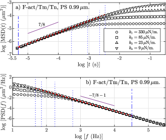
Figure 1: (Color online) a) One dimensional particle mean-squared displacement (MSD) and b) Power spectral density (PSD) for $1\,$mg/ml F-actin solution with Tm and Tn for an optically trapped polystyrene (PS) BSA microparticle with $a=0.99\,\mu$m. The data have been blocked in 10 bins per decade. Errors are very small and are not plotted for clarity. Trap forces are indicated in the legend. Regression lines ( ) are calculated under the limits defined by the dashed lines, the purple line ( ) is a guide for the eye indicating the power-law exponent $\alpha=7/8$.

The timescales contained in (1) are valid for Newtonian fluids, but the analogous expressions for a power-law fluid depend on unknown parameters related to viscosity of the medium and the friction memory kernel Grebenkov (2011). The experimental time limits are, therefore, calculated empirically, according to the general behavior of the calculated statistical quantities, by adding multiplying factors to the Newtonian time scales, $\tau_{k}$ and $\tau_{f}$. Then, the top limit for the MSD is defined as $f_{k}\,\tau_{k}$, while the bottom limit is $f_{f}\,\tau_{f}$. The $f_{f}$ factor is fixed to $f_{f}=5$ because of the position of the $|$VAF$|(t)$ minimum in the first zero-crossing value. The factor related to $\tau_{k}=6\pi\eta a/k$ is also set to $f_{k}=5$, to perform the linear regression far enough from the influence of the elastic plateau. The $k$ value has to be modified for taking into account not only the contribution from the optical trap, but also the elastic component of the fluid. The elastic modulus for this fluid is estimated to be $G^{0}\sim 1\,$Pa (see section III.1), hence $k\approx k_{i}+6\pi aG^{0}$, where $k_{i}$ is the applied trap stiffness ($i=1\cdots 4$). The corresponding limits applied to the PSD$(f)$ and the loss modulus $G^{\prime\prime}(\omega)$ (section III.1) are $\omega_{f}$ = $2\pi/(f_{f}\,\tau_{f})$ and $\omega_{k}$ = $2\pi/(f_{k}\,\tau_{k})$. For the $|$VAF$|(t)$, the short-time limit is the same: $f_{f}\,\tau_{f}$. The top limit, $f_{k}\,\tau_{k}$, is limited by the data noise on the $|$VAF$|(t)$, which is set to $f_{k}=0.03$.

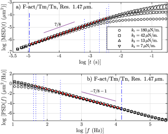
Figure 2: (Color online) a) One dimensional particle mean-squared displacement (MSD) and b) Power spectral density (PSD) for $1\,$mg/ml F-actin solution with Tm and Tn for an optically trapped melamine resin microparticle with $a=1.47\,\mu$m. The rest of the information about data and lines is the indicated in Fig. 1.

In Fig. 1, we show an example of MSD and PSD curves for a micron-sized PS tracer bead optically-trapped with different trap stiffnesses and immersed in a solution of the F-actin/Tm/Tn complex. The dashed lines are the limits of the linear regressions, which are shown in red color. Apparently, the power-law behaviors for PS BSA-added depleted particles generate a clear $\alpha=7/8$ value from both statistical quantities. However, the detail of the calculations shows a small dependence on the applied optical trap. Such a difference between $\alpha$ values is appreciable in F-actin alone, but it is mitigated when adding Tm, and even a bit more when adding Tm and Tn. This subtle effect can be appreciated in the data plotted in Fig. 6c) and d), at the end of this manuscript, and confirms the stabilization of the actin filament through Tm/Tn. Fig. 2 plots similar curves, but for chemically-inert melamine particles with a size similar to $\l_{e}$. The purple line acting as a guide for the eye may indicate that 7/8 is the correct exponent, but the calculations return exponents in the range $0.85-0.80$, with a unclear dependence on optical forces. Even in this case, the data shown in Fig. 6 (blank points) are less dispersed when using Tm or Tm/Tn.

From the macro-rheometry and compatible methods, such as two-point microrheology, the observed exponent for a F-actin solution of semiflexible polymers, like the one used in these experiments, should be $\alpha=3/4$ Morse (1997); Gittes and MacKintosh (1998). However, there are two competing anisotropic contributions in the fluctuations of the semiflexible polymer: parallel or perpendicular to the local orientation Everaers et al. (1999), where the longitudinal fluctuations behave as $\left<\delta r_{\shortparallel}\right>\sim t^{7/8}$ Gardel et al. (2004). The 3/4 exponent appears when there is no dependency of the grade of entanglement of the filament in the network Addas et al. (2004) and, at high frequencies, when the entanglements and the rigidity of the polymers only allow to move the filaments laterally Palmer et al. (1999).

The 7/8 value of the power-law exponent has previously been detected in similar F-actin experiments. In detail: $\alpha=0.86\pm 0.04$ was obtained by diffusing wave spectroscopy (DWS) for PS BSA-coated particles with $a=1.6\,\mu$m and actin concentration $c_{A}=0.8\,$mg/ml Chae and Furst (2005); $1>\alpha>3/4$ for silica spheres with radii $a=0.6\,\mu$m in $1\,$mg/ml non-crosslinked F-actin solutions Koenderink et al. (2006), $\alpha\sim 0.9$ for entangled F-actin solution for interferometric microrheology with two optically-trapped particles Atakhorrami et al. (2008), $\alpha=0.88\pm 0.04$ in cardiac thin filaments with added calcium at $3.66\,\mu$M with PS $0.489\,\mu$m tracers Tassieri et al. (2008), a 7/8 value for $G^{\prime\prime}(\omega)$ in optically trapped silica beads of $a=2.5\,\mu$m at $0.1\,$mg/ml concentration Tassieri et al. (2012), 7/8 exponent for a trapped melanine resin bead of $a=1.5\,\mu$m at $0.5\,$mg/ml Grebenkov et al. (2013), and an exponent apparently in the range $1>\alpha>3/4$ for $G^{\prime\prime}(\omega)$ for one-point microrheology of a collection of bead sizes for $c_{A}=1\,$mg/ml Atakhorrami et al. (2014). Apart from experiments, the exponent 7/8 also appears in the stress autocorrelation function of semiflexible polymers simulated by Brownian dynamics Dimitrakopoulos et al. (2001), in the polymer fluctuations parallel to the local axis Liverpool and Maggs (2001), in tension dynamics of extensible wormlike chains Obermayer and Erwin (2009), and using a wormlike-chain model of semiflexible chains with internal friction Hiraiwa and Ohta (2010).

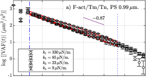
(a)

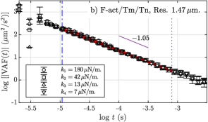
(b)

Figure 3: (Color online) Absolute values of the velocity autocorrelation function, $|\text{VAF}|$ at $1\,$mg/ml F-actin with Tm and Tn solution for a) polystyrene (PS) BSA microparticle with $a=0.99\,\mu$m and b) melamine resin with $a=1.47\,\mu$m. The errors are calculated by the blocking method. Data points for the different trap stiffnesses are indicated in the legends. Regression lines ( ) are calculated under the limits defined by the blue dashed lines: top ( ) and lower limits ( ). The purple lines ( ) are a guide for the eye indicating the averaged power-law exponent $\beta$ in each case.

Regarding the velocity autocorrelation function, Fig. 3 plots these curves for PS BSA-coated (a) and melanine resin (b) particles, for the available optical forces, when the fluid is composed by the F-actin/Tm/Tn complex. The observed behavior is again analogous to F-actin alone (see Ref. Domínguez-García et al. (2022)) and no difference is observed in the $\beta$ exponent for different fluids (see averaged values in Table 1). We have already mentioned the presence of three types of power-law exponents in this function, although in graphs like Fig. 3 we can only observe the $\beta$ exponent, which only appears in the presence of viscoelasticity. We obtain that the averaged exponents are $\beta\sim 1.05$ for chemically-inert resin particles (Fig. 3b)) and $\beta\sim 0.87$ for depleted PS tracers (Fig. 3a)).

The viscoelastic power-law behavior in the VAF of a microsphere in an actin solution was already observed by Xu et al. Xu et al. (1998). The value they calculated for the exponent in intermediate time-scales was $\beta=-0.97$, compatible with the value we obtain for chemically-inert resin particles. They also obtain the short and long times exponents: $-1.95$ and $-1.75$, respectivetely, very differenciated from the Newtonian $-1.5$ and $-3.5$, although a more rapid decay of the long-time tail exponent is expected because stress propagation is faster than diffusive in a viscoelastic fluid Atakhorrami et al. (2008). Theoretically, Grebenkov and Vahabi Grebenkov and Vahabi (2014) deduced explicit expressions for the statistical quantities considered here when the friction memory kernel decays as a power-law. Using their phenomenological model, which included inertial and hydrodynamic effects at short-times and optical trapping at long times, they obtained power-law scaling in the VAFs at intermediate times for several $\alpha$ exponents. Using the data from the figures provided in their publication (Fig. 4 (c)), we obtain that the $\beta$ exponents are: $\beta\sim 0.98$ for $\alpha=7/8$, and $\beta\sim 1.17$ for $\alpha=3/4$. A simple interpolation between these pairs of values provides $\beta=1.08$ for $\alpha=0.81$, which agrees with our experimental values for resin particles. In any case, the first exponent matches well with the experimental value observed by Xu et al., indicating a actual value of $\alpha=7/8$ instead of the expected 3/4. The results of those studies confirm the atypical character of the exponent measured here for depleted particles. Additional research in the interaction of the depletion forces of spherical probes under external forces is required for its physical-chemical explanation.

III.1 1P Microrheology

The mechanical behavior of these F-actin networks is a classical example of semiflexible polymers in solution. To obtain the viscoelastic modulus from a tracer bead immersed in the fluid, we have to convert the statistical quantities relation to the particle’s motion into the complex modulus $G^{*}(\omega)=G^{\prime}(\omega)+iG^{\prime\prime}(\omega)$, where $G^{\prime\prime}(\omega)$ is the loss modulus and $G^{\prime}(\omega)$ is the elastic or storage modulus. The standard formalism in microrheology for this calculation is to employ the measured MSD through the Mason-Weitz (MW) approach based on the generalized Stokes-Einstein relation (GSER) Mason et al. (1997) concurrent with Mason’s approximation Mason (2000) to obtain:

$$G^{*}(\omega)=\frac{k_{B}T}{i\omega\pi a\overline{\left<\Delta r^{2}(\omega)\right>}},$$ (2)

where $\overline{\left<\Delta r^{2}(\omega)\right>}$ is the one-side Fourier transform of the MSD. A second classic methodology for obtaining $G^{*}$ is using the measured PSD of the probe and Kramer-Kronig (KK) integrals. The power-spectrum density is related to the imaginary part of the complex susceptibility, $\alpha^{*}(\omega)=\alpha^{\prime}(\omega)+i\alpha^{\prime\prime}(\omega)$, by $\alpha^{\prime\prime}(\omega)=\omega$ PSD$(\omega)/4k_{B}T$. The real part of $\alpha(\omega)$ can be obtained by the known Kramer-Kronig expression:

$$\alpha^{\prime}(\omega)=\frac{2}{\pi}\,\int^{\infty}_{0}\cos(\omega t)\,dt\int^{\infty}_{0}\alpha^{\prime\prime}(z)\sin(zt)\,dz.$$ (3)

Then, the complex modulus is calculated by $G^{*}(\omega)=1/6\pi a\,\alpha^{*}(\omega)$. The main issue in this method is the calculation of (3), because of the high-values of the frequencies inside of the integrals, applied to a finite range of data. We evaluate eq. (3) by using the efficient Filon methods developed by Shampine for integrating oscillatory integrals Shampine (2013), providing analogous results to the MW method Domínguez-García et al. (2020).

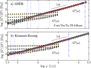
Figure 4: (Color online) Storage modulus, $G^{\prime}(\omega)$ (smaller points) and loss modulus, $G^{\prime\prime}(\omega)$, for an optically trapped polystyrene (PS) BSA microparticle with $a=0.99\,\mu$m in F-actin/Tm/Tn complex ($c_{A}=1\,$mg/ml). a) Obtained by means of the GSER and the MSD, or b) through the Kramers-Kronig expression and the PSD (see text for details). The data symbols are the same as in Fig. 1. Regression lines are calculated under the limits defined by the dashed lines.

The validity of the microrheology calculations depends of two assumptions: i) the applicability of the Stokes equation, which assumes that the bead moves in a continuum mechanical environment ($a>\xi$), and ii) the material should be in thermal equilibrium, or sufficiently close to it, as it might happen in materials undergoing a chemical reaction, gelation or degradation Furst and Squires (2017). Any variation of these conditions will generate strange effects in the results when obtaining $G^{*}$. Besides, in both described methodologies (MW and KK) a characteristic breakup for the elastic modulus, $G^{\prime}$, at high frequencies is observed. This behavior, which appears decades before the influence of the Nyquist frequency Nishi et al. (2018), is likely to occur because of the greater sensitivity of the cosine calculation at low values of $t$. Additionally, the Mason’s approximation in the Mason-Weitz method uses $\alpha(s)\equiv\left.{(d\ln\text{MSD}(t)/\ln t)}\right|_{t=1/s}$, to locally expand the MSD around the frequency of interest $s$. As Mason commented in his work, if $\alpha\sim 1$ over a large temporal range, the estimate for the dominant $G^{\prime\prime}(\omega)$ is excellent, but $G^{\prime}(\omega)$ degrades. Besides, it is known that the elastic component is very sensitive to artifacts Savin and Doyle (2007); Domínguez-García and Rubio (2013), and great care has to be applied regarding the interpretation of the calculated elastic modulus at higher frequencies. Therefore, we only maintain calculations for the elastic modulus, $G^{\prime}(\omega)$, at $\omega<10\,$kHz and we focus on the behavior of the loss modulus, $G^{\prime\prime}(\omega)$, in terms of very high-frequency microrheology of the fluid.

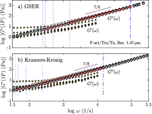
Figure 5: (Color online) $G^{\prime}(\omega)$ (small points) and $G^{\prime\prime}(\omega)$ for an optically trapped melamine resin microparticle with $a=1.47\,\mu$m in F-actin/Tm/Tn complex ($c_{A}=1\,$mg/ml). a) From GSER (MW) and b) Kramers-Kronig expression. The data symbols are the same as in Fig. 2 and 4.

Figs. 4 and 5 show two examples of the calculation of the micromechanical properties using the described microrheological methods and both tracer beads for suspensions of the F-actin/Tm/Tn complex. The general behavior is very similar using the two types of particles and it is viscoelastic: at small frequencies, a small plateau modulus appears; but at high frequencies, the fluid is liquid-like because the loss modulus, $G^{\prime\prime}(\omega)$, dominates the elastic one, $G^{\prime}(\omega)$. The loss modulus follows the expected power-law behavior $G^{\prime\prime}(\omega)\sim\omega^{\alpha}$, where the exponents $\alpha$ are calculated using the same procedure explained before (in Figs. 4 and 5, red lines are the regression lines and the dashed lines indicate the limits for each one).

Figure 6: (Color online) Values of the calculated power-law exponent $\alpha$ for each experiment (not averaged) in function of the trap stiffness, $k$. For clarity, we exclude the horizontal error bars and we limit the plots to the exponents extracted from the one dimensional particle mean-squared displacement (MSD) and the loss modulus ($G^{\prime\prime}$) calculated using the GSER. We show $\alpha$ values from the two type of particles: Polystyrene (PS) BSA $a=0.99\,\mu$m, from the MSD ( ) and from $G^{\prime\prime}$ ( ); melamine resin $a=1.47\,\mu$m, from the MSD ( ) and from $G^{\prime\prime}$ ( ). a) Measurements performed in water for control. b) F-actin. c) F-actin with tropomyosin (Tm). d) F-actin with Tm and troponin (Tn). See the texts for details in the composition of the fluids. The dashed lines ( ) indicate the values $\alpha=7/8=0.875$ and $\alpha=3/4=0.75$.

An important rheological quantity is the value of the elastic modulus at low frequency, i.e., the plateau modulus $G^{0}$. The elastic modulus $G^{\prime}(\omega)$ observed in Figs. 4 and 5 is almost constant until $1\,$kHz Gardel et al. (2003), where it begins to follow the power-law tendency of the loss modulus. This constant behavior appears because the polymers are sterically hindered by other filaments at length scales in the order of $le$, the entanglement length. Each $G^{\prime}(\omega)$ depends on the applied optical force by its elastic component $G^{\prime}_{k}=k/6\pi a$. With our optical tweezers, particles immersed in water with $a=0.99\,\mu$m generate an elastic response $G_{k}=0.5\,$Pa for the weakest optical force, and $G_{k}=18\,$Pa for the strongest ($G_{k}=0.25\,$Pa and $G_{k}=7\,$Pa, respectively, when $a=1.47\,\mu$m). For the weakest optical forces, Figs. 4 and 5 show values $G^{\prime}<1\,$Pa, but the optical forces clearly affect the elastic behavior of the fluid, effect which begins to vanish at high frequencies because the elastic modulus tends to collapse to a single unique curve. As a reference, in similar experiments, for the cardiac thin filaments with calcium for $1\,$mg/ml actin concentration, $G^{\prime}(\omega_{0})<0.1\,$Pa is obtained Tassieri et al. (2008). In general, the accepted value for F-actin alone at $1\,$mg/ml is $G^{0}\sim 1\,$Pa, but with variations depending on preparation, type of polymerization and storage Xu et al. (1998). However, many different investigations in the rheology of physiological F-actin solutions provide $G^{\prime}(\omega_{0})<1\,$Pa, where $\omega_{0}$ is the lowest available frequency. For example: by means of different techniques in rheometry Hinner et al. (1998); Schmidt et al. (2000); Goldmann (2000); Koenderink et al. (2009), using Dynamic Wave Scattering (DWS) Gisler and Weitz (1999), 1P and 2P microrheology Crocker et al. (2000); Gardel et al. (2003); Koenderink et al. (2006); He and Tang (2011).

The general behavior of the local complex modulus observed in Figs. 4 and 5 for the skeletal thin filament is analogous to the one we have obtained for F-actin alone (see Ref. Domínguez-García et al. (2022)). The main difference is the same we observed using MSD and PSD: there is a reduction of the dispersion for the exponents values in F-actin/Tm and F-actin/Tm/Tn in comparison with F-actin alone (see triangle data in Fig. 6), something which can be understood as an improvement in the stabilization of the filaments. The effect of the reported increasing of filament stiffness by a 50% is observed in rheological measurements at very low frequencies Goldmann (2000) appearing for elastic and loss modulus smaller than $0.1\,$Pa, and, at frequencies greater than $10\,$Hz (molar ratio of 7:1:1, same as here), the differences in the complex modulus in the presence or absence of Tm/Tn are apparently negligible.

Table 1: All averages of the power-law exponents for all optical forces. The parentheses in the numbers are concise notation for the numerical value of the standard uncertainty.

Material	Bead	$a$($\mu$m)	$k$($\mu$N/m)	$\left<\alpha_{\text{MSD}}\right>$	$\left<\alpha_{\text{PSD}}\right>$	$\left<\alpha_{\text{GSER}}\right>$	$\left<\alpha_{\text{KK}}\right>$	$\left<\beta_{\text{VAF}}\right>$
Actin	PS(BSA)	$0.99$	$9\pm 4$	$0.873(11)$	$0.869(13)$	$0.883(9)$	$0.857(13)$	$0.90(4)$
Actin	PS (BSA)	$0.99$	$23\pm 3$	$0.861(6)$	$0.848(7)$	$0.874(6)$	$0.851(8)$	$0.885(16)$
Actin	PS (BSA)	$0.99$	$85\pm 17$	$0.843(8)$	$0.836(10)$	$0.866(7)$	$0.864(9)$	$0.811(23)$
Actin	PS (BSA)	$0.99$	$330\pm 140$	$0.81(4)$	$0.80(4)$	$0.83(4)$	$0.855(16)$	$0.89(7)$
Actin Tm.	PS (BSA)	$0.99$	$9\pm 4$	$0.879(2)$	$0.875(3)$	$0.888(2)$	$0.862(3)$	$0.884(12)$
Actin Tm.	PS (BSA)	$0.99$	$23\pm 3$	$0.862(6)$	$0.847(6)$	$0.876(6)$	$0.854(4)$	$0.84(3)$
Actin Tm.	PS (BSA)	$0.99$	$85\pm 17$	$0.86(3)$	$0.85(3)$	$0.876(15)$	$0.871(17)$	$0.80(3)$
Actin Tm.	PS (BSA)	$0.99$	$330\pm 140$	$0.807(13)$	$0.79(3)$	$0.845(9)$	$0.853(12)$	$0.88(5)$
Actin Tm. Tn.	PS (BSA)	$0.99$	$9\pm 4$	$0.888(3)$	$0.877(4)$	$0.887(2)$	$0.858(7)$	$0.91(2)$
Actin Tm. Tn.	PS (BSA)	$0.99$	$23\pm 3$	$0.875(1)$	$0.867(3)$	$0.885(1)$	$0.865(1)$	$0.879(14)$
Actin Tm. Tn.	PS (BSA)	$0.99$	$85\pm 17$	$0.86(2)$	$0.856(3)$	$0.878(13)$	$0.875(4)$	$0.81(3)$
Actin Tm. Tn.	PS (BSA)	$0.99$	$330\pm 140$	$0.839(10)$	$0.836(17)$	$0.862(7)$	$0.868(5)$	$0.82(4)$
Actin	Resin	$1.47$	$7\pm 2$	$0.81(3)$	$0.81(2)$	$0.82(4)$	$0.782(19)$	$1.09(7)$
Actin	Resin	$1.47$	$13\pm 3$	$0.816(16)$	$0.808(15)$	$0.829(18)$	$0.790(17)$	$1.08(7)$
Actin	Resin	$1.47$	$42\pm 5$	$0.81(3)$	$0.81(3)$	$0.82(3)$	$0.80(3)$	$1.05(7)$
Actin	Resin	$1.47$	$180\pm 70$	$0.79(3)$	$0.80(3)$	$0.80(4)$	$0.82(4)$	$1.05(8)$
Actin Tm.	Resin	$1.47$	$7\pm 2$	$0.815(13)$	$0.806(13)$	$0.827(12)$	$0.781(12)$	$1.06(4)$
Actin Tm.	Resin	$1.47$	$13\pm 3$	$0.824(7)$	$0.815(7)$	$0.837(7)$	$0.795(1)$	$1.010(16)$
Actin Tm.	Resin	$1.47$	$42\pm 5$	$0.814(11)$	$0.808(8)$	$0.829(13)$	$0.801(13)$	$1.00(5)$
Actin Tm.	Resin	$1.47$	$180\pm 70$	$0.803(11)$	$0.803(13)$	$0.819(14)$	$0.822(16)$	$0.97(4)$
Actin Tm. Tn.	Resin	$1.47$	$7\pm 2$	$0.837(12)$	$0.827(15)$	$0.847(10)$	$0.808(9)$	$1.02(3)$
Actin Tm. Tn.	Resin	$1.47$	$13\pm 3$	$0.83(2)$	$0.82(2)$	$0.844(18)$	$0.806(18)$	$1.01(4)$
Actin Tm. Tn.	Resin	$1.47$	$42\pm 5$	$0.819(13)$	$0.813(14)$	$0.832(13)$	$0.806(18)$	$1.01(3)$
Actin Tm. Tn.	Resin	$1.47$	$180\pm 70$	$0.76(3)$	$0.784(2)$	$0.76(5)$	$0.802(12)$	$1.053(3)$

Finally, we comment Fig. 6, which has already been mentioned beforehand in this manuscript. This figure shows a multiple plot of the calculated $\alpha$ values for the two types of particles with their dependency with the trap stiffness values. For clarity, it only includes $\alpha$ values obtained through the MSD and $G^{\prime\prime}$ calculated by the method of GSER and Mason’s approximation. For control purpose, we include reference water measurements in Fig. 6a), returning values of $\alpha\approx 1$. Remarkably, some data near to 3/4 appears in Fig. 6b), something which might cause confusion regarding the actual value of $\alpha$ if fewer measurements were made. As mentioned in the text, the values of $\alpha$ are closer to the 7/8 line when adding Tm, and even a little more when adding Tm and Tn, confirming that the F-actin/Tm/Tn complex is able to slightly modify the mechanical response of the filaments, even in the local microscale. In Table 1, we summarize all the averaged values for the power-law exponents, including the exponent $\beta$ for the VAF, for the different experiments performed in F-actin, F-actin/Tm, and F-actin/Tm/Tn. In that table, we can see clearly how $\beta$ (last column) does not depend on the optical trap, only on the type of trapped particle.

IV Conclusions

In this work, we generalize the results from Ref. Domínguez-García et al. (2022) by providing further information of the experimental results of optical trapping interferometry (OTI) detecting the local longitudinal fluctuations of F-actin filaments Domínguez-García et al. (2022). We provide details about OTI set-up, the tracer beads materials, and the methodology of calculation of statistical and microrheological magnitudes. In the following appendix, we include detailed information on the process of data calibration used for the figures showed in this work.

We have focused here on the experiments with added skeletal tropomyosin and troponin to F-actin. This skeletal thin filament, which has a role in muscle contraction through its interaction with myosin, is expected to be stiffer than F-actin alone. We have not detected an increase of stiffness because our experimental system does not detect the very low-frequency elastic plateau, and we also have to take into account the limitations induced by one-particle microrheology and the influence of the optical elastic force in the fluid itself. However, the detected high-frequency regime allows to calculate the characteristic power-law exponent values of these semiflexible polymers, results summarized in Figure 6 and Table 1. The plot of all the results for the power-law exponent values shows how the dispersion around the 7/8 value is reduced when including Tm or Tm/Tn to the F-actin network, effect that we interpret as a micro-mechanical stabilization of the filaments.

V Acknowledgments

P.D.G acknowledges support aid by grant PID2020-117080RB-C54 funded by MCIN/AEI/10.13039/501100011033. J.R.P. acknowledges support from National Institutes of Health grant R01 HL128683. A.A. acknowledges funding from the Swiss National Science Foundation through project PP00P2_202661.

*

Appendix A Calibration of example curves

One main issue analyzing OTI data is how to convert the measured signals to units of displacements of the trapped-Brownian beads, i.e., how to calibrate and obtain the volts-to-meter conversion factor. This calibration is straightforward when the bead is immersed in Newtonian fluids Grimm et al. (2012); Butykai et al. (2015, 2017); if the mechanical behavior of the fluid is simple, like a Kevin-Voigt fluid Domínguez-García et al. (2020); or by using the method of the double flow chamber Bertseva et al. (2012); Domínguez-García et al. (2014). Classic methods are comparing with the MSD characteristic plateau at long-times, MSD$(\infty)=2k_{B}T/k$, if the optical trap stiffness is already known, or using the Lorentzian form of the PSD Addas et al. (2004).

One calibration method in non-Newtonian fluids uses the averaged values of $\left<k\right>$ measured in water, in analogy with the double flow chamber method Domínguez-García et al. (2016). Then, the low-frequency elastic modulus of the fluid should be greater than the elastic component from the optical trap, i.e., $G^{\prime}(0)>G^{\prime}_{k}=k/6\pi a$. If not, the optical trap may modify the fluid itself and this calibration method is not correct Tassieri (2015). In other words, if the trap stiffness generates an elastic component in the order of the storage modulus of the fluid, the microrheological measurements for $G^{\prime}$ at low frequencies are not representative of the surrounding medium. As we have analyzed already in this paper, we assume that $G^{\prime}(\omega_{0})<1\,$Pa for F-actin solutions at $1\,$mg/ml.

With our optical tweezers, particles with $a=0.99\,\mu$m generate $G_{k}=18\,$Pa for the strongest forces ($G_{k}=7\,$Pa for $a=1.47\,\mu$m). Therefore, the elastic modulus plateau measured in the fluid, when using the strongest trap, appears because of the external force. This is why calibration can be made using the averaged water value for that optical force. Conversely, the lower values of $G_{k}$ are in the order of the expected values for $G^{0}$ in these F-actin solutions, in agreement with the fact that the bead could be moved inside the formed fluid using the optical tweezers in any performed experiment.

All the curves shown here and in Ref. Domínguez-García et al. (2022) have been calibrated using the following steps: i) GSER is calculated from the MSDs, and a calibration factor for the curve with the strongest optical trap ($k_{1}$) is obtained by comparing it with its $G_{k}$ value measured in water; ii) if we assume that the bead is in thermal equilibrium and that the short-time bevahior reflects the polymeric structure, all curves should collapse at very short-time values Domínguez-García et al. (2016), thus we can calculate a calibration factor for the other optical forces, iii) the PSD and VAFs are calibrated using these factors, and finally the microrheological quantities are calculated once again.

References

- Bershitsky et al. (1997) S. Y. Bershitsky, A. K. Tsaturyan, O. N. Bershitskaya, G. I. Mashanov, P. Brown, R. Burns, and M. A. Ferenczi, Nature 388, 186 (1997).
- Bao and Suresh (2003) G. Bao and S. Suresh, Nat. Mater. 2, 715 (2003).
- Ebashi et al. (1971) S. Ebashi, T. Wakabayashi, and F. Ebashi, J. Biomech. 69, 441 (1971).
- Khaitlina (2015) S. Y. Khaitlina, Int. Rev. Cell Mol. Biol. 318, 255 (2015).
- Perry (2003) S. V. Perry, J. Muscle Res. Cell Motil. 24, 593 (2003).
- Potter and Gergely (1975) J. D. Potter and J. Gergely, J Biol Chem. 250, 4628 (1975).
- Götter et al. (1996) R. Götter, G. K., E. Frey, B. M., and E. Sackmann, Magnetohydrodynamics 29, 30 (1996).
- Jeney et al. (2010) S. Jeney, F. Mor, R. Koszali, L. Forró, and V. T. Moy, Nanotechnology 21 (2010).
- Franosch et al. (2011) T. Franosch, M. Grimm, M. Belushkin, F. M. Mor, G. Foffi, L. Forró, and S. Jeney, Nature (London) 478, 85 (2011).
- Mason and Weitz (1995) T. G. Mason and D. A. Weitz, Phys. Rev. Lett. 74, 1250 (1995).
- Waigh (2005) T. A. Waigh, Rep. Prog. Phys. 68, 685 (2005).
- Atakhorrami et al. (2014) M. Atakhorrami, G. H. Koenderink, J. F. Palierne, F. C. MacKintosh, and C. F. Schmidt, Phys. Rev. Lett. 112, 088101 (2014).
- Schmidt et al. (2000) F. G. Schmidt, B. Hinner, and E. Sackmann, Phys. Rev. E 61, 5646 (2000).
- Buchanan et al. (2005) M. Buchanan, M. Atakhorrami, J. F. Palierne, and C. F. Schmidt, Macromolecules 38, 8840–8844 (2005).
- Domínguez-García et al. (2022) P. Domínguez-García, J. R. Pinto, A. Akrap, and S. Jeney, “Colloid-polymer interplay in the local longitudinal fluctuations of f-actin solutions,” (2022).
- Lukić et al. (2005) B. Lukić, S. Jeney, C. Tischer, A. J. Kulik, L. Forró, and E. L. Florin, Phys. Rev. Lett. 95, 160601 (2005).
- Faucheux and Libchaber (1994) L. P. Faucheux and A. J. Libchaber, Phys. Rev. E 49, 5158 (1994).
- Jeney et al. (2008) S. Jeney, B. Lukić, J. A. Kraus, T. Franosch, and L. Forró, Phys. Rev. Lett. 100, 240604 (2008).
- Valentine et al. (2004) M. T. Valentine, Z. E. Perlman, M. L. Gardel, J. H. Shin, and P. Matsudaira, Biophys. J. 86, 4004 (2004).
- Meyer et al. (2006) A. Meyer, A. Marshall, B. G. Bush, and E. M. Furst, J. Rheol. 50, 77 (2006).
- Samiul et al. (2012) A. Samiul, C. A. Rega, and H. Jankevics, Rheol. Acta , 329 (2012).
- McGrath et al. (2000) J. L. McGrath, J. H. Hartwig, and S. C. Kuo, Biophys. J. 79, 3258 (2000).
- Chae and Furst (2005) B. A. Chae and M. F. Furst, Langmuir , 3084 (2005).
- Pardee and A (1982) J. D. Pardee and S. J. A, Methods Enzymol. 85, 164 (1982).
- Wulf et al. (1979) E. Wulf, A. Deboben, F. A. Bautz, H. Faulstich, and T. Wieland, Proc. Natl. Acad. Sci. USA. 76, 4498 (1979).
- Potter (1982) J. D. Potter, Methods Enzymol. 85, 241 (1982).
- Irving (2012) M. Irving, in Comprehensive Biophysics, edited by E. H. Egelman (Elsevier, Amsterdam, 2012) pp. 191–225.
- Egelman (1985) E. H. Egelman, J. Muscle Res. Cell Motil. 6, 129 (1985).
- Schmidt et al. (1989) C. F. Schmidt, M. Baermann, G. Isenberg, and E. Sackmann, Macromolecules 22, 3638 (1989).
- Ott et al. (1993) A. Ott, M. Magnasco, A. Simon, and A. Libchaber, Phys. Rev. E 48, R1642 (1993).
- Isambert et al. (1995) H. Isambert, P. Venier, A. C. Maggs, A. Fattoum, R. Kassab, D. Pantaloni, and M. F. Carlier, J Biol Chem. 270, 11437 (1995).
- Kaufmann et al. (1992) S. Kaufmann, J. Käs, W. H. Goldmann, E. Sackmann, and G. Isenberg, FEBS Letters 314, 203 (1992).
- Palmer et al. (1999) A. Palmer, T. G. Mason, J. Xu, S. C. Kuo, and D. Wirtz, Biophys. J. 76, 1063 (1999).
- Addas et al. (2004) K. M. Addas, C. F. Schmidt, and J. X. Tang, Phys. Rev. E 70, 021503 (2004).
- Isambert and Maggs (1996) H. Isambert and A. C. Maggs, Magnetohydrodynamics 29, 1036 (1996).
- He and Tang (2011) J. He and J. X. Tang, Phys. Rev. E 83, 041902 (2011).
- Chen et al. (2003) D. T. Chen, E. R. Weeks, J. C. Crocker, M. F. Islam, R. Verma, J. Gruber, A. J. Levine, T. C. Lubensky, and A. G. Yodh, Phys. Rev. Lett. 90, 108301 (2003).
- Donath et al. (1997) E. Donath, A. Krabi, M. Nirschl, V. M. Shilov, M. I. Zharkikh, and B. Vincent, J. Chem. Soc., Faraday Trans. 93, 115 (1997).
- Flyvbjerg and Petersen (1989) H. Flyvbjerg and H. G. Petersen, J. Chem. Phys. 91, 461 (1989).
- Huang et al. (2011) R. Huang, I. Chavez, K. M. Taute, B. Lukic, S. Jeney, M. G. Raizen, and E. L. Florin, Nat. Phys. 7, 576 (2011).
- Alder and Wainwright (1967) B. J. Alder and T. E. Wainwright, Phys. Rev. Lett. 18, 988 (1967).
- Franosch and Jeney (2009) T. Franosch and S. Jeney, Phys. Rev. E 79, 031402 (2009).
- Langevin, P. (1908) Langevin, P., C.R. Acad. Sci. Paris 146, 530 (1908).
- Clercx, H. J. H. and Schram, P. P. J. M. (1992) Clercx, H. J. H. and Schram, P. P. J. M., Phys. Rev. A 46, 1942 (1992).
- Grebenkov (2011) D. S. Grebenkov, Phys. Rev. E 83, 061117 (2011).
- Morse (1997) D. C. Morse, Phys. Rev. E 58, R1237 (1997).
- Gittes and MacKintosh (1998) F. Gittes and F. C. MacKintosh, Phys. Rev. E 58, R1241 (1998).
- Everaers et al. (1999) R. Everaers, F. Jülicher, A. Ajdari, and A. C. Maggs, Phys. Rev. Lett. 82, 3717 (1999).
- Gardel et al. (2004) M. L. Gardel, J. H. Shin, F. C. MacKintosh, L. Mahadevan, P. Matsudaira, and D. A. Weitz, Science 304, 1301 (2004).
- Koenderink et al. (2006) G. H. Koenderink, M. Atakhorrami, F. C. MacKintosh, and C. F. Schmidt, Phys. Rev. Lett. 96, 138307 (2006).
- Atakhorrami et al. (2008) M. Atakhorrami, D. Mizuno, G. H. Koenderink, T. B. Liverpool, F. C. MacKintosh, and C. F. Schmidt, Phys. Rev. E 77, 061508 (2008).
- Tassieri et al. (2008) M. Tassieri, R. M. Evans, L. Barbu-Tudoran, J. Trinick, and T. A. Waigh, Biophys. J. 94, 2170 (2008).
- Tassieri et al. (2012) M. Tassieri, R. M. L. Evans, R. L. Warren, N. J. Bailey, and J. M. Cooper, New J. Phys. 14 (2012).
- Grebenkov et al. (2013) D. S. Grebenkov, M. Vahabi, E. Bertseva, L. Forró, and S. Jeney, Phys. Rev. E 88, 040701 (2013).
- Dimitrakopoulos et al. (2001) P. Dimitrakopoulos, J. F. Brady, and Z. G. Wang, Phys. Rev. E 64, 050803 (2001).
- Liverpool and Maggs (2001) T. B. Liverpool and A. C. Maggs, Macromolecules 34, 6064–6073 (2001).
- Obermayer and Erwin (2009) B. Obermayer and F. Erwin, Phys. Rev. E 80, 040801 (2009).
- Hiraiwa and Ohta (2010) T. Hiraiwa and T. Ohta, J. Chem. Phys. 133, 044907 (2010).
- Xu et al. (1998) J. Xu, W. H. Schwarz, J. A. Käs, T. P. Stossel, P. A. Janmey, and T. D. Pollard, Biophys. J. 74, 2731 (1998).
- Grebenkov and Vahabi (2014) D. S. Grebenkov and M. Vahabi, Phys. Rev. E 89, 012130 (2014).
- Mason et al. (1997) T. G. Mason, K. Ganesan, J. H. van Zanten, D. Wirtz, and S. C. Kuo, Phys. Rev. Lett. 79, 3282 (1997).
- Mason (2000) T. G. Mason, Rheol. Acta 39, 371 (2000).
- Shampine (2013) L. F. Shampine, Appl Math Comput. 221, 691 (2013).
- Domínguez-García et al. (2020) P. Domínguez-García, G. Dietler, L. Forró, and S. Jeney, Soft Matter 20, 4234 (2020).
- Furst and Squires (2017) E. M. Furst and T. M. Squires, Microrheology (OUP Oxford, 2017).
- Nishi et al. (2018) K. Nishi, M. L. Kilfoil, C. F. Schmidt, and F. C. MacKintosh, Soft Matter 14, 3716 (2018).
- Savin and Doyle (2007) T. Savin and P. S. Doyle, Phys. Rev. E 76, 021501 (2007).
- Domínguez-García and Rubio (2013) P. Domínguez-García and M. A. Rubio, Appl. Phys. Lett. 102, 074101 (2013).
- Gardel et al. (2003) M. L. Gardel, M. T. Valentine, J. C. Crocker, A. R. Bausch, and D. A. Weitz, Phys. Rev. Lett. 91, 158302 (2003).
- Hinner et al. (1998) B. Hinner, M. Tempel, E. Sackmann, K. Kroy, and E. Frey, Phys. Rev. Lett. 81, 2614 (1998).
- Goldmann (2000) W. H. Goldmann, Biochem. Biophys. Res. Commun. 276, 1225 (2000).
- Koenderink et al. (2009) G. H. Koenderink, Z. Dogic, F. Nakamura, P. M. Bendix, F. C. MacKintosh, J. H. Hartwig, T. P. Stossel, and D. A. Weitz, Proc. Natl. Acad. Sci. USA. 106, 15192 (2009).
- Gisler and Weitz (1999) T. Gisler and D. A. Weitz, Phys. Rev. Lett. 82, 1606 (1999).
- Crocker et al. (2000) J. C. Crocker, M. T. Valentine, E. R. Weeks, T. Gisler, P. D. Kaplan, A. G. Yodh, and D. A. Weitz, Phys. Rev. Lett. 85, 888 (2000).
- Grimm et al. (2012) M. Grimm, T. Franosch, and S. Jeney, Phys. Rev. E 86, 021912 (2012).
- Butykai et al. (2015) A. Butykai, F. M. Mor, R. Gaál, P. Domínguez-García, L. Forró, and J. S., Comput. Phys. Commun. 196, 599 (2015).
- Butykai et al. (2017) A. Butykai, P. Domínguez-García, F. M. Mor, R. Gaál, L. Forró, and J. S., Comput. Phys. Commun. 220, 507 (2017).
- Bertseva et al. (2012) E. Bertseva, D. Grebenkov, P. Schmidhauser, S. Gribkova, S. Jeney, and L. Forró, Europhys. J. E. Soft. Matter. 35, 1 (2012).
- Domínguez-García et al. (2014) P. Domínguez-García, F. Cardinaux, E. Bertseva, L. Forró, F. Scheffold, and S. Jeney, Phys. Rev. E 90, 060301 (2014).
- Domínguez-García et al. (2016) P. Domínguez-García, L. Forró, and S. Jeney, Appl. Phys. Lett. 109, 143702 (2016).
- Tassieri (2015) M. Tassieri, Soft Matter 11, 5792 (2015).