Enhancements in cross-temporal forecast reconciliation, with an application to solar irradiance forecasts

Abstract

In recent works by Yang et al. [2017a, b], and Yagli et al. [2019], geographical, temporal, and sequential deterministic reconciliation of hierarchical photovoltaic (PV) power generation have been considered for a simulated PV dataset in California. In the first two cases, the reconciliations are carried out in spatial and temporal domains separately. To further improve forecasting accuracy, in the third case these two reconciliation approaches are sequentially applied. During the replication of the forecasting experiment, some issues emerged about non-negativity and coherence (in space and/or in time) of the sequentially reconciled forecasts. Furthermore, while the accuracy improvement of the considered approaches over the benchmark persistence forecasts is clearly visible at any data granularity, we argue that an even better performance may be obtained by a thorough exploitation of cross-temporal hierarchies. To this end, in this paper the cross-temporal point forecast reconciliation approach is applied to generate non-negative, fully coherent (both in space and time) forecasts. In particular, (i) some useful relationships between two-step, iterative and simultaneous cross-temporal reconciliation procedures are for the first time established, (ii) non-negativity issues of the final reconciled forecasts are discussed and correctly dealt with in a simple and effective way, and (iii) the most recent cross-temporal reconciliation approaches proposed in literature are adopted. The normalised Root Mean Square Error is used to measure forecasting accuracy, and a statistical multiple comparison procedure is performed to rank the approaches. Besides assuring full coherence, and non-negativity of the reconciled forecasts, the results show that for the considered dataset, cross-temporal forecast reconciliation significantly improves on the sequential procedures proposed by Yagli et al. [2019], at any cross-sectional level of the hierarchy and for any temporal granularity.

1 Introduction

Traditional electricity relies heavily on fossil fuels such as coal and natural gas. Not only are they bad for the environment, but they are also limited resources. Net-zero emissions by 2050 are crucial to achieve the core Paris Agreement goals of a global average temperature rise of 1.5 degrees Celsius (United Nations, 2015), and this in turn can only be achieved if global greenhouse gas emissions are halved by the end of this decade (European Commission, 2019, United Nations, 2022). Solar power is one of the crucial production methods in the move to clean energy, and as economies of scale drive prices down, its importance will undoubtedly increase. The deployment of solar-power generation is causing total installed capacity to increase at a very high pace. Eurostat reports that the European Union added 18,224.8 MW of net capacity in 2020, compared to its 16,146.9 MW increase in 2019, registering a growth of 12.9%. At the end of 2020, the EU’s photovoltaic base stood at 136,136.6 MW, which is a 15% year-on-year increase (EurObserv’ER, 2022, p. 14).

Using solar resource as a stable source of energy is not an easy task. Estimating the solar energy potential is a key target to ensure its management in a reliable and efficient way for its integration into an electrical power grid. The prediction of solar irradiation despite its variability is particularly important as it is a precondition for (i) the management of the solar photovoltaic production through storage systems to reduce the impact of the intermittent nature of the solar resource, and (ii) the integration of the solar resource into a power grid in order to meet the local energy needs and to cope with the load fluctuations. Understanding of the need for short, mid or long term prediction (e.g., 1h, 6h or a day ahead forecasting) is growing as utilities and grid operators gain experience in dealing with solar-power sources. Increasing spatial and temporal resolution of the available forecasting models would enable grid operators to better forecast how much solar energy will be added to the grid. These efforts will improve the management of solar power’s variability and uncertainty, enabling its more reliable and cost-effective integration onto the grid.

Solar forecasting is a fast-growing sub-domain of energy forecasting (Yang et al., 2020, p. 20). We agree with the claim of (Yang et al., 2022, p. 7) that a “common misconception is that the novelty in solar forecasting should be solely revolved around forecasting methodology. Indeed, forecasting methodology is an important aspect, but it is never the only one”. Nevertheless, we think that a clear assessment of the available forecasting procedures may help in moving forward the fronteer of knowledge of this fundamental topic, generating beneficial effects on the activities of practitioners.

A major goal for solar forecasting is to provide information on future photovoltaic (PV) power generation at different locations, time scales, and horizons to power system operators (Yang et al., 2022). In recent works by Yang et al. [2017a, b], and Yagli et al. [2019], geographical, temporal, and sequential deterministic reconciliation of hierarchical PV power generation have been considered for a simulated PV dataset in California. In the first two cases, the reconciliations are carried out in spatial and temporal domains separately. To further improve prediction accuracy, in the third case these two reconciliation approaches are sequentially applied. During the replication of the forecasting experiment, some issues emerged about non-negativity and coherency (in space and/or in time) of the sequentially reconciled forecasts. Furthermore, while the accuracy improvement of the considered approaches over the benchmark persistence forecasts is clearly visible at any data granularity, we think that an even better performance may be obtained by a thorough exploitation of cross-temporal hierarchies.

Cross-temporal forecast reconciliation is a rather recent sub-domain of the general theme ‘forecast reconciliation’ (Fliedner, 2001, Athanasopoulos et al., 2009, Hyndman et al., 2011). The idea of exploiting the aggregation relationships valid both in space (cross-sectional coherency), and for different time granularities (temporal coherency) to improve the forecast accuracy of base forecasts for a hierarchical time series, was discussed in the groundbreaking papers by Kourentzes and Athanasopoulos [2019], Yagli et al. [2019], Spiliotis et al. [2020b], and Punia et al. [2020]. The relevance of the topic has been further confirmed by (i) the ISF 2020 keynote speech by prof. Hyndman [2020], (ii) the entry ‘cross-temporal hierarchies’ in the encyclopedic review on the theory and practice of forecasting by Petropoulos et al. [2022], as well as (iii) the section entitled ‘cross-temporal hierarchies’ in a recent review paper on aggregation and hierarchical approaches for demand forecasting in supply chains (Babai et al., 2022). These important contributions paved the way for the findings of Di Fonzo and Girolimetto [2021], who showed the potentiality of a number of new cross-temporal reconciliation approaches, and discussed fundamental feasibility issues, offering insights to the practitioner wishing to evaluate the effort-to-benefit ratio of using this forecasting device.

In this paper, cross-temporal point forecast reconciliation is applied to generate non-negative, fully coherent (both in space and time) forecasts of PV generated power. In particular, (i) some useful relationships between two-step, iterative and simultaneous cross-temporal reconciliation procedures are for the first time established, (ii) non-negativity issues of the final reconciled forecasts are discussed and correctly dealt with in a simple and effective way, and (iii) the most recent cross-temporal reconconciliation approaches proposed in literature are adopted. The iterative and simultaneous approaches by Di Fonzo and Girolimetto [2021], and the heuristic cross-temporal procedure proposed by Kourentzes and Athanasopoulos [2019] are applied to the base forecasts with forecast horizon of 1 day, of PV generated power at different time granularities (1 hour to 1 day), of a hierarchy consisting of 324 series along 3 levels. The normalised Root Mean Square Error is used to measure forecasting accuracy, and a statistical multiple comparison procedure is performed to rank the approaches.

The paper is organized as follows. The deterministic (point) cross-temporal forecast reconciliation framework is described in section 2, and in section 3 some useful connections between apparently different approaches are shown. The forecasting experiment of Yagli et al. [2019] is replicated and discussed in section 4, and the performance of the newly proposed forecasting approaches is presented in section 5. Conclusions follow in section 6.

2 Cross-temporal point forecast reconciliation

2.1 Problem definition

To begin with, consider the very simple example of a two-level cross-sectional hierarchy, where the top variable $X$ is equal to the sum of two bottom series, $W$ and $Z$. Further, assume that the highest time frequency the variables are observed at is quarterly, which means that by simple non-overlapping temporal aggregation of quarterly time series, semi-annual and annual time series may be obtained as well. Figure 1 gives a visual representation of such cross-temporal hierarchy for a time cycle of 1 year.

Figure 1: Complete (left) and reduced (right) cross-temporal hierarchies for a quarterly two-level hierarchical time series.

While the left panel of figure 1 shows the complete cross-temporal hierarchy, consisting of all aggregated temporal granularities which may be defined starting from quarterly data (i.e, semi-annual, and annual), in the right panel is represented its reduced version, where only the highest (quarterly) and the lowest (annual) time granularities are respectively considered. The square boxes in the figure denote the nodes of a two-level cross-sectional (contemporaneous) hierarchy, while the circles denote the nodes of the temporal hierarchies. In agreement with a standard notation in the temporal forecast reconciliation literature (Athanasopoulos et al., 2017, Yang et al., 2017b), the superscript $[k]$ denotes the temporal aggregation order for each time granularity, i.e. annual ($k=4$), semi-annual ($k=2$), and quarterly ($k=1$). The cross-sectional hierarchy is described by the aggregation relationship $X=W+Z$, which is valid for any temporal aggregation order $k\in\mathcal{K}=\{4,2,1\}$ (i.e., $x_{\tau}^{[k]}=w_{\tau}^{[k]}+z_{\tau}^{[k]}$, $\tau=1,\ldots,4/k$). Assuming $v$ alternatively equal to $x,w,z$, the temporal hierarchies describing the relationships between different time granularities of a single time series, may be expressed as

$$\begin{array}[]{rcll}v^{[4]}_{1}&=&v^{[2]}_{1}+v^{[2]}_{2}&\text{{\small the annual value is the sum of the two semi-annual values},}\\ v^{[2]}_{1}&=&v^{[1]}_{1}+v^{[1]}_{2}&\text{{\small the first half-year value is the sum of the first two quarters' values},}\\ v^{[2]}_{2}&=&v^{[1]}_{3}+v^{[1]}_{4}&\text{{\small the second half-year value is the sum of the last two quarters' values},}\\ \lx@intercol\text{and thus}\hfil\lx@intercol\\ v^{[4]}_{1}&=&v^{[1]}_{1}+v^{[1]}_{2}+v^{[1]}_{3}+v^{[1]}_{4}&\text{{\small the annual value is the sum of the four quarterly values}.}\end{array}$$

All the relationships so far can be expressed in more compact form, using matrix notation. Denote by $\textbf{y}_{\tau}^{[k]}=\begin{bmatrix}x_{\tau}^{[k]}\;w_{\tau}^{[k]}\;z_{\tau}^{[k]}\end{bmatrix}^{\prime}$ the $(3\times 1)$ vector of the observations for temporal granularity $k\in\mathcal{K}$ of the variables forming the cross-sectional hierarchy at time $\tau=1,\ldots,4/k$. The cross-sectional aggregation relationships can be described as follows:

$$x_{\tau}^{[k]}=\textbf{C}\begin{bmatrix}w_{\tau}^{[k]}\\ z_{\tau}^{[k]}\end{bmatrix},\quad\textbf{y}_{\tau}^{[k]}=\textbf{S}\begin{bmatrix}w_{\tau}^{[k]}\\ z_{\tau}^{[k]}\end{bmatrix},\quad\textbf{U}^{\prime}\textbf{y}_{\tau}^{[k]}=0,\qquad\tau=1,\ldots,\displaystyle\frac{4}{k},\quad k\in\mathcal{K},$$

where C is the cross-sectional aggregation matrix, S is the cross-sectional summing matrix, and $\textbf{U}^{\prime}$ is the zero-constraints matrix expressing the cross-sectional constraints in homogeneous form, respectively given by:

$$\textbf{C}=\begin{bmatrix}1&1\\ \end{bmatrix},\quad\textbf{S}=\begin{bmatrix}\textbf{C}\\ \textbf{I}_{2}\end{bmatrix}=\begin{bmatrix}1&1\\ 1&0\\ 0&1\end{bmatrix},\quad\textbf{U}^{\prime}=\begin{bmatrix}\textbf{I}_{1}\;\;-\textbf{C}\end{bmatrix}=\begin{bmatrix}1&-1&-1\\ \end{bmatrix},$$

with $\textbf{I}_{l}$ denoting the identity matrix of order $l$. The complete temporal aggregation relationships linking the values of a single variable (say $V$) at different time granularities, may in turn be expressed through matrices

$$\textbf{K}=\begin{bmatrix}1&1&1&1\\ 1&1&0&0\\ 0&0&1&1\end{bmatrix},\quad\textbf{R}=\begin{bmatrix}\textbf{K}\\ \textbf{I}_{4}\end{bmatrix}=\begin{bmatrix}1&1&1&1\\ 1&1&0&0\\ 0&0&1&1\\ 1&0&0&0\\ 0&1&0&0\\ 0&0&1&0\\ 0&0&0&1\end{bmatrix},\quad\textbf{Z}^{\prime}=\begin{bmatrix}\textbf{I}_{3}\;\;-\textbf{K}\end{bmatrix}=\begin{bmatrix}1&0&0&-1&-1&-1&-1\\ 0&1&0&-1&-1&0&0\\ 0&0&1&0&0&-1&-1\end{bmatrix},$$

where K is the temporal aggregation matrix, R is the temporal summing matrix, and $\textbf{Z}^{\prime}$ is the temporal zero-constraints matrix expressing the temporal constraints in homogeneous form. It follows that:

$$\begin{bmatrix}v^{[4]}_{1}\\ v^{[2]}_{1}\\ v^{[2]}_{2}\end{bmatrix}=\textbf{K}\begin{bmatrix}v^{[1]}_{1}\\ v^{[1]}_{2}\\ v^{[1]}_{3}\\ v^{[1]}_{4}\end{bmatrix}=\textbf{K}\textbf{v}^{[1]},\quad\textbf{v}=\begin{bmatrix}v^{[4]}_{1}\\ v^{[2]}_{1}\\ v^{[2]}_{2}\\ v^{[1]}_{1}\\ v^{[1]}_{2}\\ v^{[1]}_{3}\\ v^{[1]}_{4}\end{bmatrix}=\textbf{R}\textbf{v}^{[1]},\quad\textbf{Z}^{\prime}\textbf{v}=\textbf{0}_{(3\times 1)}.$$

Reduced temporal hierarchies can be obtained by simply eliminating the appropriate rows from matrix K.

To simultaneously consider cross-sectional and temporal aggregation relationships, all the nodes of the complete cross-temporal hierarchy in figure 1 can be expressed in terms of the quarterly time series $w_{\tau}^{[1]}$ and $z_{\tau}^{[1]}$, $\tau=1,\ldots,4$, according to the structural representation:

$$\textbf{y}=\textbf{F}\textbf{b}^{[1]},$$ (1)

that is

$$\underbrace{\begin{bmatrix}x_{1}^{[4]}\\ x_{1}^{[2]}\\ x_{2}^{[2]}\\ x_{1}^{[1]}\\ x_{2}^{[1]}\\ x_{3}^{[1]}\\ x_{4}^{[1]}\\ w_{1}^{[4]}\\ w_{1}^{[2]}\\ w_{2}^{[2]}\\ w_{1}^{[1]}\\ w_{2}^{[1]}\\ w_{3}^{[1]}\\ w_{4}^{[1]}\\ z_{1}^{[4]}\\ z_{1}^{[2]}\\ z_{2}^{[2]}\\ z_{1}^{[1]}\\ z_{2}^{[1]}\\ z_{3}^{[1]}\\ z_{4}^{[1]}\\ \end{bmatrix}}_{\textbf{y}}=\underbrace{\begin{bmatrix}1&1&1&1&1&1&1&1\\ 1&1&0&0&1&1&0&0\\ 0&0&1&1&0&0&1&1\\ 1&0&0&0&1&0&0&0\\ 0&1&0&0&0&1&0&0\\ 0&0&1&0&0&0&1&0\\ 0&0&0&1&0&0&0&1\\ 1&1&1&1&0&0&0&0\\ 1&1&0&0&0&0&0&0\\ 0&0&1&1&0&0&0&0\\ 1&0&0&0&0&0&0&0\\ 0&1&0&0&0&0&0&0\\ 0&0&1&0&0&0&0&0\\ 0&0&0&1&0&0&0&0\\ 0&0&0&0&1&1&1&1\\ 0&0&0&0&1&1&0&0\\ 0&0&0&0&0&0&1&1\\ 0&0&0&0&1&0&0&0\\ 0&0&0&0&0&1&0&0\\ 0&0&0&0&0&0&1&0\\ 0&0&0&0&0&0&0&1\end{bmatrix}}_{\textbf{F}}\underbrace{\begin{bmatrix}w_{1}^{[1]}\\ w_{2}^{[1]}\\ w_{3}^{[1]}\\ w_{4}^{[1]}\\ z_{1}^{[1]}\\ z_{2}^{[1]}\\ z_{3}^{[1]}\\ z_{4}^{[1]}\\ \end{bmatrix}}_{\textbf{b}^{[1]}},$$

where $\textbf{y}=\begin{bmatrix}\textbf{x}^{\prime}\;\textbf{w}^{\prime}\;\textbf{z}^{\prime}\end{bmatrix}^{\prime}$ is the vector containing the data for all variables at any temporal granularity, $\textbf{b}^{[1]}=\begin{bmatrix}\textbf{w}^{[1]\prime}\;\textbf{z}^{[1]\prime}\end{bmatrix}^{\prime}$ is the vector of the high-frequency bottom time series, and F is the cross-temporal summing matrix mapping $\textbf{b}^{[1]}$ into y. Expression (1) is the natural extension of the cross-sectional structural representation firstly shown by Athanasopoulos et al. [2009]. It relates the observations at the upper levels of both cross-sectional and temporal hierarchies, to the high-frequency bottom time series of the cross-sectional hierarchy, which are the ‘very’ bottom time series in a cross-temporal hierarchy (Di Fonzo and Girolimetto, 2021).

Besides the number of variables forming the cross sectional hierarchy ($n=3$ in the above example), two crucial aspects affecting the dimension of matrix F are (i) the temporal frequency of the highest-frequency granularity ($k=1$), and (ii) the amount of temporal granularities taken into account in the temporal hierarchy. For example, if one is interested in coherently forecasting hourly time series within a day-cycle, the complete cross-temporal summing matrix R defining all infra-day temporal granularities ($\mathcal{K}=\{24,12,8,6,4,3,2,1\}$) has dimension $(60\times 24)$, and is equal to

$$\textbf{R}=\begin{bmatrix}\textbf{1}_{24}&\textbf{I}_{2}\otimes\textbf{1}_{12}&\textbf{I}_{3}\otimes\textbf{1}_{8}&\textbf{I}_{4}\otimes\textbf{1}_{6}&\textbf{I}_{6}\otimes\textbf{1}_{4}&\textbf{I}_{8}\otimes\textbf{1}_{3}&\textbf{I}_{12}\otimes\textbf{1}_{2}&\textbf{I}_{24}\end{bmatrix}^{\prime}.$$

Matrix F is thus a large and sparse matrix of dimension $(60n\times 24n_{b})$, where $n$ is the total number of series, and $n_{b}$ is the number of bottom time series in the cross-sectional hierarchy, respectively (in the above example, $n=3$ and $n_{b}=2$). Just to give an idea, the total number of variables in the dataset analyzed in this paper (see section 4) is $n=324$, with $n_{b}=318$ bottom time series, thus matrix F has dimension ($19{,}440\times 7{,}632$). However, if the interest in forecasting at certain time granularities is low, this dimensonality issue may be mitigated by considering only part of the temporal granularities between the highest and lowest temporal frequencies. For example, if one considers only hourly and daily forecasts, the reduced F is a $(8{,}100\times 7{,}632)$ matrix, with a decrease of about 58% in the amount of matrix entries wrt its complete counterpart.

In this framework, by extending the seminal idea by Hyndman et al. [2011], a forecast reconciliation problem arises when, for the nodes of a cross-temporal hierarchy, a set of base forecasts - however obtained, and usually not aggregate consistent either in space and/or in time - are wished to be revised to fulfill the coherency relationships in space and time valid for the target data. The purpose is to improve the accuracy of the initial forecasts by combining forecasts at different aggregation levels in space and time, and by incorporating in the final forecasts the information given by cross-sectional and temporal constraints.

2.2 Notation

Suppose we want to forecast a $n$-variate high-frequency hierarchical time series $\left\{\textbf{y}_{t}^{[1]}\right\}_{t=1}^{T}$, with forecast horizon equal to the seasonal cycle $m$, (e.g., month per year, $m=12$, quarter per year, $m=4$, hour per day, $m=24$), or a multiple thereof. Given a factor $k$ of $m$, we may consider a number of temporally aggregated versions of each component of $\textbf{y}_{t}^{[1]}$, given by the non-overlapping sums of $k$ successive values, each having seasonal period equal to $M_{k}=m/k$. To avoid ragged-edge data, we assume that the total number of observations involved in the non-overlaping aggregation is a multiple of $m$, and define $N$ the number of the lowest-frequency series observations, i.e. $N=T/m$. Let $\mathcal{K}$ be the set of $p$ factors of $m$, in descending order, $\mathcal{K}=\{k_{p},k_{p-1},\ldots,k_{2},k_{1}\}$, where $k_{p}=m$ and $k_{1}=1$, and define $k^{*}=\displaystyle\sum_{j=2}^{p}k_{j}$.

Following Di Fonzo and Girolimetto [2021], denote $\textbf{Y}_{N+h}\equiv\textbf{Y}$ the $\left[n\times(k^{*}+m)\right]$ matrix of the target forecasts for any temporal granularity, with low-frequency temporal horizon $h$, given by:

$$\textbf{Y}=\left[\textbf{Y}^{[m]}\;\textbf{Y}^{[k_{p-1}]}\ldots\textbf{Y}^{[k_{2}]}\;\textbf{Y}^{[1]}\right]=\left[\begin{array}[]{c}\textbf{A}\\ \textbf{B}\end{array}\right]=\left[\begin{array}[]{ccccc}\textbf{A}^{[m]}&\textbf{A}^{[k_{p-1}]}&\ldots&\textbf{A}^{[k_{2}]}&\textbf{A}^{[1]}\\ \textbf{B}^{[m]}&\textbf{B}^{[k_{p-1}]}&\ldots&\textbf{B}^{[k_{2}]}&\textbf{B}^{[1]}\end{array}\right],$$

where $m$ is the highest available sampling frequency per seasonal cycle (i.e., max. order of temporal aggregation). Each matrix $\textbf{Y}^{[k]}=\left[\begin{array}[]{c}\textbf{A}^{[k]}\\ \textbf{B}^{[k]}\end{array}\right]$, $k\in\mathcal{K}$, contains the order-$k$ temporal aggregates of the $n_{a}$ cross-sectional upper time series $(\textbf{A}^{[k]})$, and of the $n_{b}$ cross-sectional bottom time series $(\textbf{B}^{[k]})$, respectively, with $n=n_{a}+n_{b}$. Accordingly, we define the matrix of base forecasts $\widehat{\textbf{Y}}$ as:

$$\widehat{\textbf{Y}}=\left[\widehat{\textbf{Y}}^{[m]}\;\widehat{\textbf{Y}}^{[k_{p-1}]}\ldots\widehat{\textbf{Y}}^{[k_{2}]}\;\widehat{\textbf{Y}}^{[1]}\right]=\left[\begin{array}[]{ccccc}\widehat{\textbf{A}}^{[m]}&\widehat{\textbf{A}}^{[k_{p-1}]}&\ldots&\widehat{\textbf{A}}^{[k_{2}]}&\widehat{\textbf{A}}^{[1]}\\ \widehat{\textbf{B}}^{[m]}&\widehat{\textbf{B}}^{[k_{p-1}]}&\ldots&\widehat{\textbf{B}}^{[k_{2}]}&\widehat{\textbf{B}}^{[1]}\end{array}\right].$$

While the target forecasts are expected to be aggregate-consistent both in time and space, the base forecasts are in general cross-sectionally and/or temporally incoherent, that is:

$$\textbf{U}^{\prime}\textbf{Y}=\textbf{0}_{[n_{a}\times(k^{*}+m)]}\quad\text{and}\quad\textbf{Z}^{\prime}\textbf{Y}^{\prime}=\textbf{0}_{[k^{*}\times n]},\quad\text{while}\quad\textbf{U}^{\prime}\widehat{\textbf{Y}}\neq\textbf{0}_{[n_{a}\times(k^{*}+m)]}\quad\text{and/or}\quad\textbf{Z}^{\prime}\widehat{\textbf{Y}}^{\prime}\neq\textbf{0}_{[k^{*}\times n]},$$

where $\textbf{U}^{\prime}=\begin{bmatrix}\textbf{I}_{n_{a}}\;-\textbf{C}\end{bmatrix}$ and $\textbf{Z}^{\prime}=\begin{bmatrix}\textbf{I}_{k^{*}}\;-\textbf{K}\end{bmatrix}$ are zero-constraints matrices associated to the cross-sectional and temporal constraints, respectively. Working with a single dimension (either sectional, or temporal), we may consider the multivariate generalization of the structural representations for cross-sectional (Athanasopoulos et al., 2009), and temporal (Athanasopoulos et al., 2017), hierarchies, respectively:

Cross-sectional structural representation of $k^{*}+m$ hierarchical time series

$$\textbf{y}_{\tau}^{[k]}=\textbf{S}\textbf{b}_{\tau}^{[k]},\quad\tau=1,\ldots,\frac{m}{k},\quad\rightarrow\quad\textbf{Y}^{[k]}=\textbf{S}\textbf{B}^{[k]}\quad\quad k\in\mathcal{K},$$

that is, in compact form

$$\textbf{Y}=\textbf{S}\textbf{B}\quad\rightarrow\quad\textbf{y}=\left(\textbf{S}\otimes\textbf{I}_{k^{*}+m}\right)\textbf{b},$$

where $\textbf{y}=\text{vec}\left(\textbf{Y}^{\prime}\right)$, and $\textbf{b}=\text{vec}\left(\textbf{B}^{\prime}\right)$.

Temporal hierarchies structural representation for $n$ individual time series

$$\begin{array}[]{c}\textbf{a}_{i}=\textbf{R}\textbf{a}_{i}^{[1]},\quad i=1,\ldots,n_{a}\\ \textbf{b}_{j}=\textbf{R}\textbf{b}_{j}^{[1]},\quad j=1,\ldots,n_{b}\\ \end{array}\quad\rightarrow\quad\begin{array}[]{c}\textbf{A}=\textbf{R}\textbf{A}^{[1]\prime}\\ \textbf{B}=\textbf{R}\textbf{B}^{[1]\prime}\\ \end{array},$$

that is

$$\textbf{Y}^{\prime}=\textbf{R}\textbf{Y}^{[1]\prime}\quad\rightarrow\quad\textbf{y}=\left(\textbf{I}_{n}\otimes\textbf{R}\right)\textbf{y}^{[1]},$$

where $\textbf{y}^{[1]}=\text{vec}\left({\textbf{Y}^{[1]}}^{\prime}\right)$, and R is the temporal summing matrix (Di Fonzo and Girolimetto, 2021).

2.3 Cross-temporal bottom-up reconciliation

Bottom-up is an old and classic approach in the forecast reconciliation literature (Dunn et al., 1976, Dangerfield and Morris, 1992). This approach simply consists in obtaining the upper-level series’ forecasts by summing-up the base forecasts of the bottom level series in the hierarchy. While its representation is rather straightforward when only a single dimension (either space or time) is involved, it is instructive considering how ‘bottom-up’ works with cross-temporal hierarchies. The cross-temporal bottom-up (ct$(bu)$) reconciliation of $k^{*}+m$ hierarchical time series’ base forecasts at different time granularities, may be represented as:

$$\text{vec}\left(\widetilde{\textbf{Y}}_{\text{ct}(bu)}^{\prime}\right)=\textbf{F}\text{vec}\left(\widehat{\textbf{B}}^{[1]\prime}\right)\quad\leftrightarrow\quad\widetilde{\textbf{y}}_{\text{ct}(bu)}=\textbf{F}\widehat{\textbf{b}}^{[1]},$$ (2)

where $\textbf{F}=\textbf{S}\otimes\textbf{R}$ is the cross-temporal summing matrix, with $\otimes$ denoting the Kronecker product, and $\widehat{\textbf{b}}^{[1]}=\text{vec}\left(\widehat{\textbf{B}}^{[1]\prime}\right)$ is the vector containing the base forecasts of the high-frequency bottom time series. In A it is shown that the cross-temporal bottom-up reconciliation can be tought of as a two-step sequential reconciliation approach, where either cross-sectional reconciliation of the high-frequency bottom time series base forecasts is followed by temporal reconciliation, or vice-versa. This observation opens the way to ‘partly bottom-up’ cross-temporal reconciliation approaches, where forecasts of the $n$ time series for different time granularities, and aggregation coherent only along a single dimension, are subsequently cross-temporally reconciled via simple bottom-up according to the other dimension. We call these cross-temporal forecast reconciliation approaches either ct$(rec_{te},bu_{cs}$), or ct$(rec_{cs},bu_{te}$), where ‘$rec_{te}$’ and ‘$rec_{cs}$’ denote a generic forecast reconciliation approach in time and in space, respectively.

2.4 Regression-based cross-temporal reconciliation

Let us consider the multivariate regression model

$$\widehat{\textbf{Y}}=\textbf{Y}+\textbf{E},$$

where the involved matrices have each dimension $[n\times(k^{\ast}+m)]$ and contain, respectively, the base ($\widehat{\textbf{Y}}$) and the target forecasts (Y), and the coherency errors (E) for the $n$ component variables of the hierarchical time series of interest. Consider now the vectorized version of the model, that is

$$\mathrm{vec}\left(\widehat{\textbf{Y}}^{\prime}\right)=\mathrm{vec}\left(\textbf{Y}^{\prime}\right)+\mathrm{vec}\left(\textbf{E}^{\prime}\right)\quad\Leftrightarrow\quad\widehat{\textbf{y}}=\textbf{y}+\boldsymbol{\eta},$$ (3)

where $\boldsymbol{\eta}=\mathrm{vec}\left(\textbf{E}^{\prime}\right)$ is the cross-temporal reconciliation error with zero mean and p.d. covariance matrix $\bm{\mathsf{\Omega}}_{ct}$. Assuming $\bm{\mathsf{\Omega}}_{ct}$ known, the optimal combination reconciled forecasts $\widetilde{\textbf{y}}_{\text{oct}}=\mathrm{vec}\left(\widetilde{\textbf{Y}}_{\text{oct}}^{\prime}\right)$ are found by linearly constrained minimization of the generalized least squares (GLS) objective function

$$\left(\textbf{y}-\widehat{\textbf{y}}\right)^{\prime}\bm{\mathsf{\Omega}}_{ct}^{-1}\left(\textbf{y}-\widehat{\textbf{y}}\right)\qquad\mathrm{s.t.}\;\textbf{H}^{\prime}\textbf{y}=\textbf{0},$$ (4)

where

$$\textbf{H}^{\prime}\textbf{y}=\left[\begin{array}[]{c}\textbf{U}^{\ast}\\ \textbf{I}_{n}\otimes\textbf{Z}\end{array}\right]\textbf{y}=\textbf{0}_{[n(k^{\ast}+m)\times 1]}$$

is a full row-rank cross-temporal zero-constraint matrix, with $\textbf{U}^{\ast}=\left[\textbf{0}_{(n_{a}m\times nk^{\ast})}\;\textbf{I}_{m}\otimes\textbf{U}^{\prime}\right]\textbf{P}$, and P is the $[n(k^{\ast}+m)\times n(k^{\ast}+m)]$ commutation matrix, such that $\textbf{P}\mathrm{vec}(\textbf{Y})=\textbf{y}$ (Di Fonzo and Girolimetto, 2021).

The cross-temporally reconciled forecasts according to the projection approach solution (Byron, 1978; see also van Erven and Cugliari, 2015, Wickramasuriya et al., 2019, Panagiotelis et al., 2021, Di Fonzo and Girolimetto, 2021) are given by

$$\widetilde{\textbf{y}}_{\text{oct}}=\left[\textbf{I}_{n(k^{\ast}+m)}-\bm{\mathsf{\Omega}}_{ct}\textbf{H}\left(\textbf{H}^{\prime}\bm{\mathsf{\Omega}}_{ct}\textbf{H}\right)^{-1}\textbf{H}^{\prime}\right]\widehat{\textbf{y}}=\textbf{M}_{ct}\widehat{\textbf{y}}.$$ (5)

Alternatively, they may be obtained according to the structural approach developed by Hyndman et al. [2011] for the cross-sectional framework:

$$\widehat{\textbf{y}}=\textbf{F}\boldsymbol{\beta}+\boldsymbol{\eta},$$

where $\boldsymbol{\beta}=E[\textbf{b}^{[1]}|\mathcal{I}_{T}]$ is the mean of the high-frequency bottom-level values conditional to $\mathcal{I}_{T}$, the available information up to time $T$, $\textbf{b}^{[1]}=\mathrm{vec}\left(\textbf{B}^{[1]\prime}\right)$. The structural approach forecast reconciliation formula is

$$\widetilde{\textbf{y}}_{\text{oct}}=\textbf{F}\left(\textbf{F}^{\prime}\bm{\mathsf{\Omega}}^{-1}_{ct}\textbf{F}\right)^{-1}\textbf{F}^{\prime}\bm{\mathsf{\Omega}}^{-1}_{ct}\widehat{\textbf{y}}=\textbf{F}\textbf{G}_{ct}\widehat{\textbf{y}},$$ (6)

with $\textbf{G}_{ct}=\left(\textbf{F}^{\prime}\bm{\mathsf{\Omega}}^{-1}_{ct}\textbf{F}\right)^{-1}\textbf{F}^{\prime}\bm{\mathsf{\Omega}}^{-1}_{ct}$. Di Fonzo and Girolimetto [2021] considered the following approximations for the cross-temporal covariance matrix (‘$oct$’ stands for ‘optimal cross-temporal’):

• identity: $\bm{\mathsf{\Omega}}_{ct}=\textbf{I}_{n(k^{*}+m)}$

• structural: $\bm{\mathsf{\Omega}}_{ct}=\mathrm{diag}(\textbf{F}\mathbf{1}_{mn_{b}})$

• series variance scaling: $\bm{\mathsf{\Omega}}_{ct}=\savestack{\tmpbox}{\stretchto{\scaleto{\scalerel*[\widthof{\bm{\mathsf{\Omega}}}]{\kern-0.6pt\bigwedge\kern-0.6pt}{\rule[-505.89pt]{4.30554pt}{505.89pt}}}{}}{0.5ex}}\stackon[1pt]{\bm{\mathsf{\Omega}}}{\tmpbox}_{ct,wlsv}$, that is a straightforward extension of the series variance scaling matrix presented by Athanasopoulos et al. [2017] in the temporal framework

• block-diagonal shrunk cross-covariance scaling: $\bm{\mathsf{\Omega}}_{ct}=\textbf{P}\savestack{\tmpbox}{\stretchto{\scaleto{\scalerel*[\widthof{\textbf{W}}]{\kern-0.6pt\bigwedge\kern-0.6pt}{\rule[-505.89pt]{4.30554pt}{505.89pt}}}{}}{0.5ex}}\stackon[1pt]{\textbf{W}}{\tmpbox}^{BD}_{ct,shr}\textbf{P}^{\prime}$

• block-diagonal cross-covariance scaling: $\bm{\mathsf{\Omega}}_{ct}=\textbf{P}\savestack{\tmpbox}{\stretchto{\scaleto{\scalerel*[\widthof{\textbf{W}}]{\kern-0.6pt\bigwedge\kern-0.6pt}{\rule[-505.89pt]{4.30554pt}{505.89pt}}}{}}{0.5ex}}\stackon[1pt]{\textbf{W}}{\tmpbox}^{BD}_{ct,sam}\textbf{P}^{\prime}$

• MinT-shr: $\bm{\mathsf{\Omega}}_{ct}=\hat{\lambda}\widehat{\bm{\mathsf{\Omega}}}_{ct,D}+(1-\hat{\lambda})\widehat{\bm{\mathsf{\Omega}}}_{ct}$

• MinT-sam: $\bm{\mathsf{\Omega}}_{ct}=\savestack{\tmpbox}{\stretchto{\scaleto{\scalerel*[\widthof{\bm{\mathsf{\Omega}}}]{\kern-0.6pt\bigwedge\kern-0.6pt}{\rule[-505.89pt]{4.30554pt}{505.89pt}}}{}}{0.5ex}}\stackon[1pt]{\bm{\mathsf{\Omega}}}{\tmpbox}_{ct}$

where the symbol $\odot$ denotes the Hadamard product, $\hat{\lambda}$ is an estimated shrinkage coefficient (Ledoit and Wolf, 2004), $\savestack{\tmpbox}{\stretchto{\scaleto{\scalerel*[\widthof{\bm{\mathsf{\Omega}}}]{\kern-0.6pt\bigwedge\kern-0.6pt}{\rule[-505.89pt]{4.30554pt}{505.89pt}}}{}}{0.5ex}}\stackon[1pt]{\bm{\mathsf{\Omega}}}{\tmpbox}_{ct,D}=\textbf{I}_{n(k^{\ast}+m)}\odot\widehat{\bm{\mathsf{\Omega}}}_{ct}$, and $\savestack{\tmpbox}{\stretchto{\scaleto{\scalerel*[\widthof{\bm{\mathsf{\Omega}}}]{\kern-0.6pt\bigwedge\kern-0.6pt}{\rule[-505.89pt]{4.30554pt}{505.89pt}}}{}}{0.5ex}}\stackon[1pt]{\bm{\mathsf{\Omega}}}{\tmpbox}_{ct}$ is the covariance matrix of the cross-temporal one-step ahead in-sample forecast errors. The cross-sectional point forecast reconciliation formula is obtained by assuming $m=1$ (which implies $k^{*}=0$, and $\bm{\mathsf{\Omega}}_{ct}=\textbf{W}$ is an ($n\times n$) p.d. matrix):

$$\widetilde{\textbf{y}}=\left[\textbf{I}_{n}-\textbf{W}\textbf{U}\left(\textbf{U}^{\prime}\textbf{W}\textbf{U}\right)^{-1}\textbf{U}^{\prime}\right]\widehat{\textbf{y}}=\textbf{M}_{cs}\widehat{\textbf{y}},$$

or, equivalently (Hyndman et al., 2011, Hyndman et al., 2016, Wickramasuriya et al., 2019),

$$\widetilde{\textbf{y}}=\textbf{S}\left(\textbf{S}^{\prime}\textbf{W}^{-1}\textbf{S}\right)^{-1}\textbf{S}^{\prime}\textbf{W}^{-1}\widehat{\textbf{y}}=\textbf{S}\textbf{G}_{cs}\widehat{\textbf{y}},$$

with $\textbf{G}_{cs}=\left(\textbf{S}^{\prime}\textbf{W}^{-1}\textbf{S}\right)^{-1}\textbf{S}^{\prime}\textbf{W}^{-1}$. The reconciled forecasts through temporal hierarchies for a single time series (Athanasopoulos et al., 2017) are in turn obtained by setting $n=1$ (i.e., $n_{a}=0$ and $n_{b}=1$, and $\bm{\mathsf{\Omega}}_{ct}=\bm{\mathsf{\Omega}}$ is a ($k^{*}+m\times k^{*}+m$) p.d. matrix):

$$\widetilde{\textbf{y}}=\left[\textbf{I}_{(k^{\ast}+m)}-\bm{\mathsf{\Omega}}\textbf{Z}\left(\textbf{Z}^{\prime}\bm{\mathsf{\Omega}}\textbf{Z}\right)^{-1}\textbf{Z}^{\prime}\right]\widehat{\textbf{y}}=\textbf{M}_{te}\widehat{\textbf{y}},$$

or, equivalently,

$$\widetilde{\textbf{y}}=\textbf{R}\left(\textbf{R}^{\prime}\bm{\mathsf{\Omega}}^{-1}\textbf{R}\right)^{-1}\textbf{R}^{\prime}\bm{\mathsf{\Omega}}^{-1}\widehat{\textbf{y}}=\textbf{R}\textbf{G}_{te}\widehat{\textbf{y}},$$

with $\textbf{G}_{te}=\left(\textbf{R}^{\prime}\bm{\mathsf{\Omega}}^{-1}\textbf{R}\right)^{-1}\textbf{R}^{\prime}\bm{\mathsf{\Omega}}^{-1}$. Table 1 presents some approximations for the cross-sectional and the temporal covariance matrices. Other alternatives for temporal reconciliation, exploiting possible information in the residuals’ autocorrelation, can be found in Nystrup et al. [2020] and Di Fonzo and Girolimetto [2021].

Table 1: Approximations for the cross-sectional (Hyndman et al., 2011, Hyndman et al., 2016, Wickramasuriya et al., 2019, Di Fonzo and Girolimetto, 2021) and temporal (Athanasopoulos et al., 2017, Di Fonzo and Girolimetto, 2021) covariance matrix to be used in a reconciliation approach^∗.

	Cross-sectional framework	Temporal framework
identity	cs$(ols)$: $\textbf{W}=\textbf{I}_{n}$	te$(ols)$: $\bm{\mathsf{\Omega}}=\textbf{I}_{k^{\ast}+m}$
structural	cs$(struc)$: $\textbf{W}=\mathrm{diag}(\textbf{S}\mathbf{1}_{nb})$	te$(struc)$: $\bm{\mathsf{\Omega}}=\mathrm{diag}(\textbf{R}\mathbf{1}_{m})$
series variance	cs$(wls)$: $\textbf{W}=\widehat{\textbf{W}}_{D}=\textbf{I}_{n}\odot\widehat{\textbf{W}}$	te$(wlsv)$: $\bm{\mathsf{\Omega}}=\widehat{\bm{\mathsf{\Omega}}}_{wlsv}$
MinT-shr	cs$(shr)$: $\textbf{W}=\hat{\lambda}\widehat{\textbf{W}}_{D}+(1-\hat{\lambda})\widehat{\textbf{W}}$	te$(shr)$: $\bm{\mathsf{\Omega}}=\hat{\lambda}\widehat{\bm{\mathsf{\Omega}}}_{D}+(1-\hat{\lambda})\widehat{\bm{\mathsf{\Omega}}}$
MinT-sam	cs$(sam)$: $\textbf{W}=\widehat{\textbf{W}}$	te$(sam)$: $\bm{\mathsf{\Omega}}=\widehat{\bm{\mathsf{\Omega}}}$
∗ $\widehat{\textbf{W}}$ ($\widehat{\bm{\mathsf{\Omega}}}$) is the covariance matrix of the cross-sectional (temporal) one-step ahead in-sample forecast errors, $\widehat{\bm{\mathsf{\Omega}}}_{wlsv}$ is a diagonal matrix “which contains estimates of the in-sample one-step-ahead error variances across each level” (Athanasopoulos et al., 2017, p. 64), and $\widehat{\bm{\mathsf{\Omega}}}_{D}=\textbf{I}_{k^{\ast}+m}\odot\widehat{\bm{\mathsf{\Omega}}}$.

2.5 Heuristic and iterative cross-temporal reconciliation

Kourentzes and Athanasopoulos [2019] proposed an ensemble forecasting procedure (denoted KA), that exploits the simple averaging of different forecasts. It consists in the following steps (for further details, see Di Fonzo and Girolimetto, 2021):

KA-Step 1

compute the temporally reconciled forecasts for each variable $i\in\{1,\ldots,n\}$, and arrange them in the $[n\times(k+m)]$ matrix $\widetilde{\textbf{Y}}_{\text{te}}$;

KA-Step 2

starting from $\widetilde{\textbf{Y}}_{\text{te}}$, compute the time-by-time cross-sectional reconciled forecasts for all the temporal aggregation levels ($\widetilde{\textbf{Y}}_{\text{cs}}$), and collect all the $(n\times n)$ projection matrices used to reconcile forecasts of $k$-level temporally aggregated time series, $\textbf{M}_{cs}^{[k]}$, $k\in\mathcal{K}$;

KA-Step 3

transform the step 1 forecasts once more, by computing time-by-time cross-sectional reconciled forecasts for all temporal aggregation levels using the $(n\times n)$ matrix $\overline{\textbf{M}}$, given by the average of the matrices $\textbf{M}_{\text{cs}}^{[k]}$:

$$\widetilde{\textbf{Y}}_{\text{KA}}=\left(\frac{1}{p}\sum_{k\in\mathcal{K}}\textbf{M}_{\text{cs}}^{[k]}\right)\widetilde{\textbf{Y}}_{\text{te}}=\overline{\textbf{M}}\widetilde{\textbf{Y}}_{\text{te}}.$$

Di Fonzo and Girolimetto [2021] presented an iterative approach, that produces cross-temporally reconciled forecasts by alternating forecast reconciliation along one dimension (cross-sectional or temporal), based on the first two steps of the KA approach. The iteration $j\geq 1$ can be described as follows:

Step 1

compute the temporally reconciled forecasts ($\widetilde{\textbf{Y}}_{\text{te}}^{(j)}$) for each variable $i\in\{1,\ldots,n\}$ of $\widetilde{\textbf{Y}}_{\text{cs}}^{(j-1)}$;

Step 2

compute the time-by-time cross-sectional reconciled forecasts ($\widetilde{\textbf{Y}}^{(j)}_{\text{cs}}$) for all the temporal aggregation levels of $\widetilde{\textbf{Y}}_{\text{te}}^{(j)}$.

At $j=0$, the starting values are given by $\widetilde{\textbf{Y}}_{\text{cs}}^{(0)}=\widehat{\textbf{Y}}$, and the iterates end when the entries of matrix $\textbf{D}_{\text{te}}=\textbf{Z}^{\prime}\widetilde{\textbf{Y}}^{(j)\prime}_{\text{cs}}$, containing all the temporal discrepancies, are small enough according to a suitable convergence criterion. The order of the dimensions to be reconciled in the two steps within each iteration is arbitrary (on this point, see Di Fonzo and Girolimetto, 2021): in the description above, temporal-then-cross-sectional reconciliation is iteratively performed (ite$(rec_{\text{te}},rec_{\text{cs}})$), otherwise the order may be reversed, getting cross-sectional-then-temporal reconciliation (ite$(rec_{\text{cs}},rec_{\text{te}})$).

3 Cross-temporal coherency of sequential approaches and some remarkable equivalences

In order to exploit both cross-sectional and temporal hierarchies, Yagli et al. [2019] consider two sequential reconciliation approaches: Spatial-then-Temporal-Reconciliation (STR), and Temporal-then-Spatial-Reconciliation (TSR). In the former case, cross-sectional reconciliation of the base forecasts is performed first for any temporal granularity, followed by the temporal reconciliation of the individual series’ forecasts. In the latter case, the order of application of the two reconciliation approaches is reversed, temporal reconciliation being performed first, followed by cross-sectional reconciliation. In general, one would expect that the forecasts obtained this way are different (i.e., $\widetilde{\textbf{Y}}_{TSR}\neq\widetilde{\textbf{Y}}_{TSR}$), and either cross-sectionally (TSR) or temporally (STR), but not cross-temporally, reconciled:

$$\textbf{U}^{\prime}\widetilde{\textbf{Y}}_{TSR}=\textbf{0}_{[n_{a}\times(k^{*}+m)]},\quad\textbf{Z}^{\prime}\widetilde{\textbf{Y}}_{TSR}\neq\textbf{0}_{(k^{*}\times n)},\qquad\textbf{U}^{\prime}\widetilde{\textbf{Y}}_{STR}\neq\textbf{0}_{[n_{a}\times(k^{*}+m)]},\quad\textbf{Z}^{\prime}\widetilde{\textbf{Y}}_{STR}=\textbf{0}_{(k^{*}\times n)}.$$

At this regard, we have found an interesting result, here shown as Theorem 1, according to which, if both covariance matrices used in either steps are constant across levels and time granularities, the final result (i) does not depend on the order of application of the uni-dimensional reconciliation phases, and (ii) is equivalent to that obtained through an optimal combination approach using a separable covariance matrix, i.e. with a Kronecker product structure [Genton, 2007, Werner et al., 2008, Velu and Herman, 2017].

Theorem 1.

Let $\textbf{W}^{[k]}$, $k\in\mathcal{K}$, be the cross-sectional hierarchy error covariance matrix, and $\bm{\mathsf{\Omega}}_{i}$, $i=1,\ldots,n$, the $i$-th series temporal hierarchy error covariance matrix. If $\textbf{W}^{[k]}=\textbf{W}$, $\forall k\in\mathcal{K}$, and $\bm{\mathsf{\Omega}}_{i}=\bm{\mathsf{\Omega}}$, $\forall i=1,\ldots,n$, then:

1. the iterative procedure reduces to a single (two-step) iteration to obtain cross-temporal reconciled forecasts. Furthermore,

   $$\widetilde{\textbf{Y}}_{\text{tcs}}=\widetilde{\textbf{Y}}_{\text{cst}}=\widetilde{\textbf{Y}}_{\text{seq}},$$

   where $\widetilde{\textbf{Y}}_{\text{tcs}}$ ($\widetilde{\textbf{Y}}_{\text{cst}}$) is the [$n\times(k^{\ast}+m)$] matrix of the temporal-then-cross-sectional (cross-sectional-then-temporal) reconciled forecasts;

2. Denoting $\widetilde{\textbf{Y}}_{\text{oct}}$ the optimal (in least squares sense) combination cross-temporal reconciliation approach with cross-temporal covariance matrix $\bm{\mathsf{\Omega}}_{\text{ct}}=\textbf{W}\otimes\bm{\mathsf{\Omega}}$, it is:

   $$\widetilde{\textbf{Y}}_{\text{seq}}=\widetilde{\textbf{Y}}_{\text{oct}}.$$

Proof.

B. ∎

It is worth noting that, when only constant error covariance matrices are involved in both unidimensional steps, the iterative cross-temporal reconciliation approach proposed by Di Fonzo and Girolimetto [2021] reduces to the sequential procedure proposed by Yagli et al. [2019], and gives a unique result, $\widetilde{\textbf{Y}}_{\text{seq}}$, which does not depend on the order of application of the reconciliation phases. In addition, it does exist a simple simultaneous, optimal (in least-squares sense) reconciliation approach equivalent to the above sequential forecast reconciliation procedure. Finally, it should be noted that under the constant covariance matrices assumption of the theorem, the heuristic cross-temporal reconciliation approach by Kourentzes and Athanasopoulos [2019] is equivalent to a sequential approach, since in this case the final averaging phase is not needed (more details can be found in B, after the proof of the theorem). All these results can be summarized as follows:

$$\begin{array}[]{l}\textbf{W}^{[k]}=\textbf{W},\forall k\in\mathcal{K}\\ \bm{\mathsf{\Omega}}_{i}=\bm{\mathsf{\Omega}},i=1,\ldots,n\\ \bm{\mathsf{\Omega}}_{ct}=\textbf{W}\otimes\bm{\mathsf{\Omega}}\end{array}\quad\rightarrow\quad\underbrace{\widetilde{\textbf{Y}}_{\text{KA}(tcs)}=\widetilde{\textbf{Y}}_{\text{KA}(cst)}}_{\parbox[t]{85.35826pt}{\scriptsize\centering\cite[cite]{\@@bibref{Authors Phrase1YearPhrase2}{Kourentzes2019}{\@@citephrase{[}}{\@@citephrase{]}}}\@add@centering}}=\underbrace{\widetilde{\textbf{Y}}_{\text{seq}}}_{\parbox[t]{49.79231pt}{\scriptsize\centering\cite[cite]{\@@bibref{Authors Phrase1YearPhrase2}{Yagli2019}{\@@citephrase{[}}{\@@citephrase{]}}}\@add@centering}}=\underbrace{\widetilde{\textbf{Y}}_{\text{ite}(tcs)}=\widetilde{\textbf{Y}}_{\text{ite}(cst)}=\widetilde{\textbf{Y}}_{\text{oct}}}_{\parbox[t]{85.35826pt}{\scriptsize\centering\cite[cite]{\@@bibref{Authors Phrase1YearPhrase2}{DiFonzoGiro2021}{\@@citephrase{[}}{\@@citephrase{]}}}\@add@centering}}$$

Using the covariance matrices in Table 1, we may thus establish some useful equivalences between the cross-temporal reconciliation approaches considered in Di Fonzo and Girolimetto [2021], and identify new ones:

1. oct$(ols)$: $\bm{\mathsf{\Omega}}_{\text{ct}}=\textbf{I}_{n(k^{\ast}+m)}$

   equivalent to seq/KA/ite$(ols_{te},ols_{cs})$, and seq/KA/ite$(ols_{cs},ols_{te})$, with $\textbf{W}=\textbf{I}_{n}$, $\bm{\mathsf{\Omega}}=\textbf{I}_{k^{\ast}+m}$.

2. oct$(struc)$: $\bm{\mathsf{\Omega}}_{\text{ct}}=\mathrm{diag}\left(\textbf{F}\mathbf{1}_{mn_{b}}\right)$

   equivalent to seq/KA/ite$(struc_{te},struc_{cs})$, and seq/KA/ite$(struc_{cs},struc_{te})$, with $\textbf{W}=\mathrm{diag}\left(\textbf{S}\mathbf{1}_{n_{b}}\right)$, $\bm{\mathsf{\Omega}}=\mathrm{diag}\left(\textbf{R}\mathbf{1}_{m}\right)$.

3. oct$(ols_{cs},struc_{te})$: $\bm{\mathsf{\Omega}}_{ct}=\mathrm{diag}\left[(\textbf{I}_{n}\otimes\textbf{R})\mathbf{1}_{mn_{b}}\right]$

   equivalent to seq/KA/ite$(ols_{cs},struc_{te})$, with $\textbf{W}=\textbf{I}_{n}$, $\bm{\mathsf{\Omega}}=\mathrm{diag}\left(\textbf{R}\mathbf{1}_{m}\right)$.

4. oct$(struc_{cs},ols_{te})$: $\bm{\mathsf{\Omega}}_{ct}=\mathrm{diag}\left[(\textbf{S}\otimes\textbf{I}_{k^{\ast}+m})\mathbf{1}_{mn_{b}}\right]$

   equivalent to seq/KA/ite$(struc_{cs},ols_{te})$, with $\textbf{W}=\mathrm{diag}\left(\textbf{S}\mathbf{1}_{n_{b}}\right)$, $\bm{\mathsf{\Omega}}=\textbf{I}_{k^{\ast}+m}$.

All the procedures considered so far make use of very simple covariance matrices, not using the information coming from the in-sample forecast errors. At this regard, another interesting result is that the iterative reconciliation procedure where both cross-sectional and temporal reconciliation are performed using diagonal covariance matrices, computed using the one-step-ahead in-sample forecast errors (i.e., cs$(wls)$ and te$(wlsv)$), ‘converges’ to the optimal combination reconciliation approach oct$(wlsv)$ (Di Fonzo and Girolimetto, 2021), irrespective of the order of application of the unidimensional reconciliation steps. In other terms:

$$\widetilde{\textbf{Y}}_{\mathrm{ite}(wlsv_{te},wls_{cs})}\simeq\widetilde{\textbf{Y}}_{\mathrm{ite}(wls_{cs},wlsv_{te})}\simeq\widetilde{\textbf{Y}}_{\mathrm{oct}(wlsv)},$$

where the quality of the approximation solely depends on the convergence criterion: the lower the tolerance value $\delta$ (see section 2.5), the better the approximation will be. An empirical support to this result is given by figure 2, showing the Frobenius norm of the difference between the matrices of the reconciled forecasts using ite$(wlsv_{te},wls_{cs})$ with decreasing tolerance values $\delta$, and oct$(wlsv)$, in the 350 replications of the forecasting experiment described in section 4.

In summary, when the considered diagonal covariance matrices are used in cross-sectional and temporal reconciliation phases, the iterative cross-temporal reconciliation approach is equivalent to a specific optimal combination cross-temporal approach. We argue that in practical application it is convenient to adopt the optimal combination version of a cross-temporal procedure, rather than its iterative counterpart, because the numerical results have better accuracy, and the computing time is often lower, mostly if the programming codes exploit sparse matrices tools (Davis, 2006).

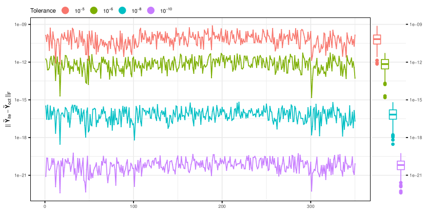
Figure 2: Frobenius norm of the difference between the matrices of the reconciled forecasts using ite$(wlsv_{te},wls_{cs})$ and oct$(wlsv)$, with different tolerance value $\delta$. 350 replications of the forecasting experiment described in section 4.

4 Replication and assessment of the forecasting experiment of Yagli et al. (2019)

The dataset used in this study, called PV324, is the same used by Yang et al. [2017a, b], and Yagli et al. [2019]. It refers to 318 simulated PV plants in California, whose hourly irradiation data are organized in three levels (figure 3):

• $\mathcal{L}_{0}$: 1 time series for the Independent System Operator (ISO), given by the sum of the 318 plant series;

• $\mathcal{L}_{1}$: 5 time series for the Transmission Zones (TZ), each given by the sum of 27, 73, 101, 86, and 31 plants, respectively;

• $\mathcal{L}_{2}$: 318 bottom time series at plant level (P).

Figure 3: PV324 hierarchy

Following Yang et al. [2017b] and Yagli et al. [2019], we perform a forecasting experiment with fixed length window of 14 days (i.e., 336 hours), forecast horizon of two days, and forecasting evaluation taking into account only the day-2 forecasts. These settings are coherent with the forecast operational submission requirements of CAISO, the public corporation managing power grid operations in California (Makarov et al., 2011, Kleissl, 2013). For the 318 hourly time series, numerical weather prediction (NWP) forecasts generated by 3TIER (3TIER, 2010) are used as base forecasts. All the remaining base forecasts, for the six $\mathcal{L}_{0}$ and $\mathcal{L}_{1}$ time series at any time granularity $k\in\mathcal{K}$, and for the $\mathcal{L}_{2}$ 2-3-4-6-8-12-24 hours time series, are computed using the automatic ETS forecasting procedure of the R-package forecast (Hyndman et al., 2021), not controlling for possible negative forecasts. Furthermore, day-ahead persistence is used as the reference model (PERS):

$$\widehat{y}_{T+h|T,\;PERS}^{[1]}=y_{T+h-48}^{[1]}.$$

Given the lead time of 48h, the day-ahead persistence takes the measurements made at day -2 as the forecasts for the operating day (Yagli et al., 2019, p. 394). Benchmark forecasts at any level of the spatial hierarchy and for any temporal granularity are obtained through cross-temporal bottom-up of the 318 hourly bottom time series, that is:

$$\widetilde{\textbf{y}}_{PERS_{bu}}={\textbf{F}}\widehat{\textbf{b}}_{PERS}^{[1]}=\text{vec}\left(\widetilde{\textbf{Y}}_{PERS_{bu}}^{\prime}\right).$$

It is worth noting that the benchmark forecasts are always non-negative, and both spatially and temporally coherent. Furthermore, these important properties are valid also for the forecasts obtained by cross-temporal bottom-up reconciliation of the 318 hourly bottom time series’ NWP forecasts 3TIER:

$$\widetilde{\textbf{y}}_{3TIER_{bu}}={\textbf{F }}\widehat{\textbf{b}}_{3TIER}^{[1]}=\text{vec}\left(\widetilde{\textbf{Y}}_{3TIER_{bu}}^{\prime}\right).$$

In light of the results provided in section 3, the eight STR and TSR sequential reconciliations proposed by Yagli et al. [2019] reduce to the following four approaches: oct($ols$), oct($ols_{cs},struc_{te}$), oct($struc_{cs},ols_{te}$), oct($struc$). In addition, Yagli et al. [2019] consider other four Temporal-then-Spatial-Reconciliation approaches, called TSR${}_{\mathcal{L}_{2}}$, where the temporal reconciliation is applied only to the 318 plant level series’ base forecasts. In this case, although constant matrices are used in either reconciliation steps, theorem 1 no longer holds, and the obtained forecasts are temporally incoherent, as we show in the following. In order to distinguish these approaches from the conventional sequential techniques, we call them te${}_{ols_{2}}$+cs_ols, te${}_{struc_{2}}$+cs_ols, te${}_{ols_{2}}$+cs_struc, te${}_{struc_{2}}$+cs_ols, respectively.

4.1 Non-negativity and aggregation consistency issues

Unlike PERS_bu and 3TIER_bu, the other approaches considered by Yagli et al. [2019] produce some negative reconciled forecasts. Looking at table 2, we note that negative hourly forecasts have been produced in all 350 replications of the forecasting experiment, and there are some cases (in a range within 4 and 11 replications out of 350) where negative daily forecasts are produced as well. Furthermore, the base forecasts are generally cross-temporally incoherent (i.e., in space and/or in time), and the sequential TSR${}_{\mathcal{L}_{2}}$ approaches proposed by Yagli et al. [2019] are temporally incoherent. This can be visually appreciated from figure 4, showing the boxplots from the distribution of the gross cross-sectional and temporal discrepancies registered in the 350 replications of the forecasting experiment, computed as (Di Fonzo and Girolimetto, 2021):

$$\begin{array}[]{rl}\text{Cross-sectional gross discrepancy:}&d_{\text{cs}}=||\textbf{U}^{\prime}\widehat{\textbf{Y}}||_{1}\\ \text{Temporal gross discrepancy:}&d_{\text{te}}=||\textbf{Z}^{\prime}\widehat{\textbf{Y}}^{\prime}||_{1}\end{array},$$

where $||\textbf{X}||_{1}=\sum_{i,j}|x_{i,j}|$. For truly cross-temporally reconciled forecasts, neither cross-sectional nor temporal discrepancies are present, that is $d_{cs}=d_{te}=0$.

Table 2: Summary informations on the negative forecasts produced by the procedures considered by Yagli et al. (2019) in the forecasting experiment. Replications with at least a negative forecast (# rep), number of series (# series) with at least a negative forecast in a single replication (min and max), and min and max negative values found in all replications (values). Hourly and daily forecasts, forecast horizon: operating day.

Approach	# rep (350)	# series (324)		values		# rep (350)	# series (324)		values
		min	max	min	max		min	max	min	max
	Hourly forecasts					Daily forecasts
base+	350	4	6	-15.617	-0.000	11	0	35	-51.205	-0.006
oct$(ols$)	350	109	324	-69.165	-0.000	11	0	60	-29.615	-0.001
oct$(ols_{cs},struc_{te})$	350	137	324	-20.739	-0.000	11	0	33	-10.363	-0.000
oct$(struc_{cs},ols_{te})$	350	91	324	-17.961	-0.000	6	0	28	-8.915	-0.008
oct$(struc)$	350	89	324	-14.292	-0.000	4	0	11	-1.020	-0.026
te$(ols_{2})$+cs$(ols)$∗	350	42	324	-12.993	-0.000	10	0	72	-15.037	-0.018
te$(struc_{2})$+cs$(ols)$∗	350	36	324	-12.994	-0.000	10	0	71	-14.791	-0.005
te$(ols_{2})$+cs$(struc)$∗	350	144	324	-7.526	-0.000	10	0	43	-12.969	-0.005
te$(struc_{2})$+cs$(struc)$∗	350	124	324	-7.642	-0.000	5	0	31	-7.042	-0.002
+ The approach produces spatial and temporal incoherent forecasts.
∗ The approach produces temporal incoherent forecasts.

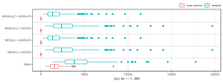
Figure 4: Base forecasts and TSR${}_{\mathcal{L}_{2}}$ reconciled forecasts: cross-sectional (cs, in red) and temporal (te, in blue) discrepancies.

In this case, forecast reconciliation may thus generate physically unreasonable values. Furthermore, if coherency is wished, the apparently innocuous practice of setting possible negative forecasts to zero is not advisable, since incoherence in sectional and/or time dimensions would be produced. To overcome the above limitations, in section 5 we propose a simple operational strategy, able to generate fully reconciled non-negative forecasts.

4.2 Forecast evaluation

Following Yagli et al., 2019, the accuracy of the considered approaches is measured in terms of normalised Root Mean Square Error (nRMSE), and Forecast Skill score:

$$\text{nRMSE}_{i,j}^{[k]}=\displaystyle\frac{\sqrt{\displaystyle\frac{1}{L}\displaystyle\sum_{l=1}^{L}\left(\widetilde{y}_{i,j,l}^{[k]}-y_{i,l}^{[k]}\right)^{2}}}{\displaystyle\frac{1}{L}\displaystyle\sum_{l=1}^{L}y_{i,l}^{[k]}},\qquad\text{Forecast Skill}_{i,j}^{[k]}=1-\frac{\text{nRMSE}_{i,j}^{[k]}}{\text{nRMSE}_{i,0}^{[k]}},$$ (7)

where $i=1,\ldots,n$, denotes the series, $k\in\mathcal{K}$, $j=0,\ldots,J$, denotes the forecasting approach ($j=0$ for the reference model PERS), and $L=nrep\cdot\displaystyle\frac{m}{k}$, where $nrep=350$ is the number of the forecasting experiment replications. Forecast Skill can be either negative (approach is worse than the reference model) or positive (approach is better than the reference model). From table 3 it appears that on average all the considered forecasting approaches improve on the benchmark PERS_bu, in a range between 9.2% (oct$(ols)$ for the 5 $\mathcal{L}_{1}$ level series’ hourly forecasts) and 38.3% (3TIER_bu for the $\mathcal{L}_{0}$ total series’ daily forecasts). The forecasting accuracy indices for each Transmission Zone forecasts are reported in table 4.

Table 3: Forecast accuracies (nRMSE %) and skills over the PERS_bu benchmark of base forecasts and sequential reconciliation approaches. Free reconciliation procedures considered by Yagli et al. [2019], Tables 2, 3, p. 395. Hourly (H) and Daily (D) forecasts, forecast horizon: operating day. Bold entries identify the best performing approach.

	$\mathcal{L}_{0}$		$\mathcal{L}_{1}$		$\mathcal{L}_{2}$		$\mathcal{L}_{0}$		$\mathcal{L}_{1}$		$\mathcal{L}_{2}$
	H	D	H	D	H	D	H	D	H	D	H	D
	$nRMSE(\%)$						forecast skill
PERSbu	34.62	20.23	43.15	24.57	59.75	30.65	0	0	0	0	0	0
3TIERbu	26.03	12.48	33.95	16.75	53.46	25.19	0.248	0.383	0.213	0.318	0.105	0.178
base+	27.85	18.17	34.24	20.94	53.46	25.82	0.196	0.102	0.206	0.148	0.105	0.158
oct($ols$)	30.69	17.91	39.17	21.74	51.54	26.73	0.113	0.115	0.092	0.115	0.137	0.128
oct$(ols_{cs},struc_{te})$	28.74	17.33	35.48	20.82	49.32	26.14	0.170	0.143	0.178	0.152	0.175	0.147
oct$(struc_{cs},ols_{te})$	28.26	16.96	35.19	20.61	48.20	25.46	0.184	0.162	0.184	0.161	0.193	0.169
oct$(struc)$	26.71	16.24	33.11	19.64	46.74	24.73	0.228	0.197	0.233	0.201	0.218	0.193
te$(ols_{2})$+cs$(ols)$∗	27.80	17.96	34.36	21.80	48.52	26.71	0.197	0.112	0.204	0.113	0.188	0.129
te$(struc_{2})$+cs$(ols)$∗	27.80	17.95	34.34	21.79	47.77	26.36	0.197	0.113	0.204	0.113	0.201	0.140
te$(ols_{2})$+cs$(struc)$∗	27.02	17.24	33.40	20.62	47.76	25.98	0.219	0.148	0.226	0.161	0.201	0.152
te$(struc_{2})$+ cs$(struc)$∗	26.17	16.68	32.44	19.96	46.25	25.03	0.244	0.176	0.248	0.188	0.226	0.183
+ The approach produces spatial and temporal incoherent forecasts.
∗ The approach produces temporal incoherent forecasts.

Table 4: Forecast accuracies (nRMSE %) and skills over the PERS_bu benchmark of base forecasts and sequential reconciliation approaches for the series at $\mathcal{L}_{1}$ level. Free reconciliation procedures considered by Yagli et al. [2019], Tables 2, 3, p. 395. Hourly (H) and Daily (D) forecasts, forecast horizon: operating day. Bold entries identify the best performing approach.

	TZ1		TZ2		TZ3		TZ4		TZ5
	H	D	H	D	H	D	H	D	H	D
	$nRMSE(\%)$
PERSbu	28.72	16.12	40.27	22.40	46.48	26.96	52.82	29.75	47.44	27.62
3TIERbu	22.81	10.43	33.34	16.72	34.01	17.06	46.40	22.80	33.16	16.75
base+	22.41	13.55	32.05	18.70	35.14	21.95	44.94	26.89	36.67	23.58
oct($ols$)	29.27	14.89	34.58	19.25	39.55	22.91	47.30	26.50	45.16	25.15
oct$(ols_{cs},struc_{te})$	24.26	13.93	32.32	18.47	36.69	21.78	43.89	25.30	38.81	23.59
oct$(struc_{cs},ols_{te})$	23.44	13.50	32.89	18.83	37.42	22.33	44.76	25.97	38.90	23.49
oct$(struc)$	22.00	12.81	30.92	17.82	34.79	20.94	42.02	24.50	35.83	22.12
te$(ols_{2})$+cs$(ols)$∗	22.95	15.46	32.06	19.23	35.12	22.38	44.93	26.91	36.73	25.02
te$(struc_{2})$+cs$(ols)$∗	22.93	15.46	32.05	19.22	35.11	22.37	44.92	26.90	36.70	25.00
te$(ols_{2})$+cs$(struc)$∗	22.11	13.36	31.40	18.70	34.70	21.93	42.97	26.06	35.82	23.06
te$(struc_{2})$+ cs$(struc)$∗	21.58	13.00	30.48	18.09	33.58	21.18	41.86	25.21	34.69	22.32
	forecast skill
PERSbu	0	0	0	0	0	0	0	0	0	0
3TIERbu	0.206	0.353	0.172	0.254	0.268	0.367	0.121	0.234	0.301	0.394
base+	0.220	0.159	0.204	0.165	0.244	0.186	0.149	0.096	0.227	0.146
oct($ols$)	-0.019	0.076	0.141	0.141	0.149	0.150	0.104	0.109	0.048	0.089
oct$(ols_{cs},struc_{te})$	0.155	0.136	0.197	0.176	0.211	0.192	0.169	0.150	0.182	0.146
oct$(struc_{cs},ols_{te})$	0.184	0.163	0.183	0.159	0.195	0.172	0.153	0.127	0.180	0.149
oct$(struc)$	0.234	0.205	0.232	0.205	0.251	0.223	0.204	0.177	0.245	0.199
te$(ols_{2})$+cs$(ols)$∗	0.201	0.041	0.204	0.141	0.244	0.170	0.149	0.095	0.226	0.094
te$(struc_{2})$+cs$(ols)$∗	0.202	0.041	0.204	0.142	0.245	0.170	0.150	0.096	0.227	0.095
te$(ols_{2})$+cs$(struc)$∗	0.230	0.171	0.220	0.165	0.253	0.187	0.187	0.124	0.245	0.165
te$(struc_{2})$+ cs$(struc)$∗	0.249	0.194	0.243	0.192	0.277	0.215	0.208	0.153	0.269	0.192
+ The approach produces spatial and temporal incoherent forecasts.
∗ The approach produces temporal incoherent forecasts.

We observe that:

• 3TIER_bu gives the best forecasting performance for the total series ($\mathcal{L}_{0}$) at any temporal granularity, the second best being te$(struc_{2})$+cs$(struc)$.

• The approach te$(struc_{2})$+cs$(struc)$ ranks first for 4 out of the 5 hourly upper series at level $\mathcal{L}_{1}$, whereas at daily level 3TIER_bu ‘wins’ again. The performance of oct$(struc)$ results very similar to that of te$(struc_{2})$+cs$(struc)$.

• te$(struc_{2})$+cs$(struc)$ and oct$(struc)$ show the best performance for the 318 bottom time series at any temporal granularity, with a slight prevalence of oct$(struc)$ (for $k\geq 3$), plus oct$(struc)$ forecasts are cross-temporally coherent.

• Unlike te$(struc_{2})$+ cs$(struc)$, 3TIER_bu forecasts are always non-negative, and coherent both in space and time with the forecasts at any granularity.

• For these reasons, 3TIER_bu should be considered as a challenging competitor in the evaluation of the newly proposed procedures (section 5).

To give a complete picture of the evaluation results for hourly and daily forecasts, in figure 5 the Multiple Comparison with the Best (MCB) Nemenyi tests are shown (Koning et al., 2005, Kourentzes and Athanasopoulos, 2019, Makridakis et al., 2022). This allows to establish if the forecasting performances of the considered techniques are significantly different. At daily level, oct$(struc)$ ranks first, and is significantly better than the other forecasting approaches, with te$(struc_{2})$+cs$(struc)$ at the second place. This result is reversed at hourly level: te$(struc_{2})$+cs$(struc)$ ranks first and is significantly better than all the other approaches, with oct$(struc)$ at the second place. However, it should be recalled that the forecasts produced by te$(struc_{2})$+cs$(struc)$ are not temporally coherent, which means that the sum of the hourly forecasts does not match with the corresponding daily forecasts (see figure 4).

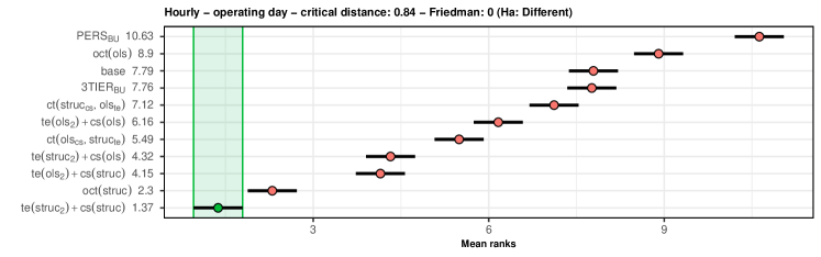
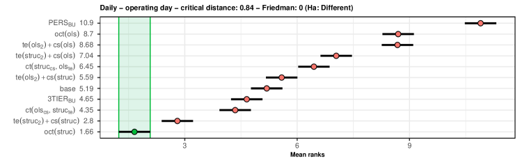
Figure 5: MCB Nemenyi test results: average ranks and 95% confidence intervals. The free reconciliation approaches considered by Yagli et al. [2019] are sorted vertically according to the nRMSE% mean rank. Hourly (top panel), and Daily (bottom panel) forecasts for $\mathcal{L}_{0},\mathcal{L}_{1},\mathcal{L}_{2}$ levels (324 series). Forecast horizon: operating day. The mean rank of each approach is displayed to the right of their names. If the intervals of two forecast reconciliation approaches do not overlap, this indicates a statistically different performance. Thus, approaches that do not overlap with the green interval are considered significantly worse than the best, and vice-versa.

Limiting ourselves to consider fully coherent reconciled forecasts, the scatter plots of the 324 couples of nRMSE(%) for oct$(struc)$ vs., respectively, PERS_bu and 3TIER_bu (figure 6), show that the most performing regression-based cross-temporal reconciliation approach improves uniformly on the benchmark, and in the majority of cases on 3TIER_bu, particularly at hourly level ($k=1$), where the 89% of the variables register an improvement in nRMSE. However, it is worth noting that at daily level, this value decreases to 49%, which means that the NWP forecasts may still play a role at lower time granularity.

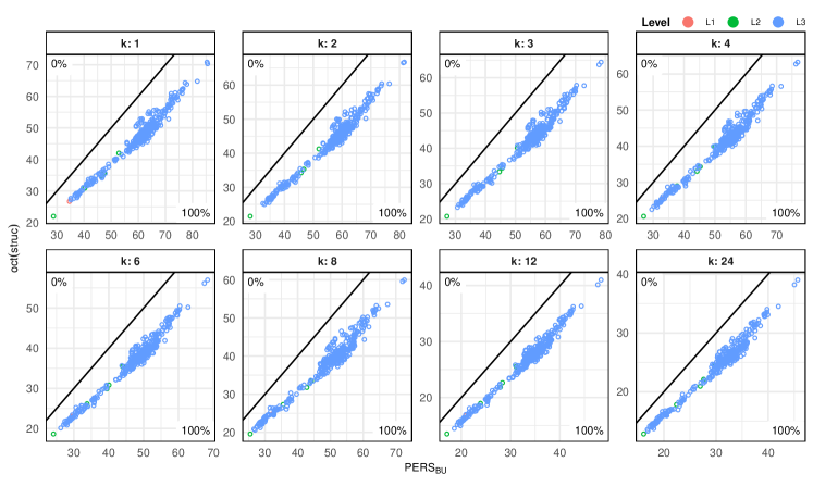
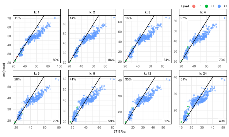
Figure 6: Comparison of nRMSE(%) between PERS_bu and ct$(struc)$ (top panel), and between 3TIER_bu and ct$(struc)$ (bottom panel). The black line represents the bisector, where the nRMSE’s for both approaches are equal. On the top-left (bottom-right) corner of each graph, the percentage of points above (below) the bisector is reported.

5 Extended analysis: non-negative cross-temporal reconciliation

In this section, we explore the performance of forecast reconciliation approaches able to produce non-negative PV forecasts, both temporally and spatially coherent. For this reason, among the approaches proposed by Yagli et al. [2019], we consider the reference benchmark PERS_bu, the NWP base forecasts 3TIER_bu, and oct$(struc)$. These approaches are then compared with the following 7 cross-temporal forecasting procedures:

• KA$(wlsv_{te},wls_{cs})$: the heuristic approach by Kourentzes and Athanasopoulos [2019], using te$(wlsv)$ in the first step, and cs$(wls)$ in the second, respectively;

• ct$(wlsv_{te},bu_{cs})$, ct$(struc_{te},bu_{cs})$, ct$(wls_{cs},bu_{te})$, and ct$(struc_{cs},bu_{te})$: partly bottom-up cross temporal reconciliation (see section 2.3) of the high frequency bottom time series’ reconciled forecasts according to, respectively, te$(wlsv)$, te$(struc)$, cs$(wls)$, and cs$(struc)$;

• oct$(wlsv)$ and oct$(bdshr)$: optimal (in least squares sense) cross-temporal forecast reconciliation approaches using the in-sample forecast errors (Di Fonzo and Girolimetto, 2021).

5.1 Non negative forecast reconciliation: sntz

Each approach, when used in its ‘free’ version, i.e., without considering non-negative constraints in the linearly constrained quadratic program (4), is not guaranteed to always produce non-negative reconciled forecasts (see section 4.1). This fact may be an issue for the analyst, since in many practical situations negative forecasts could have no meaning, thus undermining the quality of the results found and the conclusions thereof. In what follows, we consider a simple heuristic strategy to avoid negative reconciled forecasts, without using any sophisticated, and time consuming, numerical optimization procedure. More precisely, possible negative values of the free reconciled high-frequency bottom time series forecasts are set to zero. Denote $\widetilde{\textbf{B}}^{[1]}_{0}$ the matrix containing the non-negative reconciled forecasts produced by a ‘free’ approach, and the ‘zeroed’ ones. The complete vector of non-negative cross-temporal reconciled forecasts is computed as the cross-temporal bottom-up aggregation of $\widetilde{\textbf{b}}^{[1]}_{0}=\text{vec}\left[\left(\widetilde{\textbf{B}}^{[1]}_{0}\right)^{\prime}\right]$, that is, according to expression (2):

$$\widetilde{\textbf{y}}_{0}=\textbf{F}\widetilde{\textbf{b}}^{[1]}_{0}.$$

We call set-negative-to-zero (sntz) this simple, and quick device to obtain non negative reconciled forecasts. While it certainly increases the forecasting accuracy of the high-frequency bottom time series forecasts wrt the ‘free’ counterparts, this does not hold true in general for the upper level series forecasts. In addition, even if the originally reconciled forecasts are obtained according to an unbiased approach, the sntz-reconciled forecasts are no more unbiased, like the non-negative forecasts obtained through numerical optimization procedures (Wickramasuriya et al., 2020). However, in practical situations the differences between the results produced by the sntz heuristic, and those obtained through a numerical optimization procedure could be negligible. For example, for the dataset and the forecasting experiment in hand, we have found that the forecasting performance of the non-negative reconciliation approaches through the non-linear optimization procedure osqp (Stellato et al., 2020) implemented in FoReco (Girolimetto and Di Fonzo, 2022), is basically the same as the one obtained with the sntz heuristic. Table 5 shows the nRMSE(%) of the reconciled forecasts through the oct($struc$) approach in both free and non-negative (sntz and osqp) variants. It is worth noting that the simple sntz heuristic always gives the lowest nRMSE(%), independently of the temporal granularity of the forecasts.

Table 5: Forecast accuracy (nRMSE%) of free and non-negative reconciled forecasts using the oct($struc$) approach. All temporal aggregation orders are considered, from hourly ($k=1$) to daily ($k=24$). Forecast horizon: operating day. Bold entries identify the best approach.

non-negative	$k$: temporal aggregation order
reconciliation	1	2	3	4	6	8	12	24
$\mathcal{L}_{0}$ (1 series)
free	26.71	26.35	25.67	25.57	23.03	24.80	16.74	16.24
sntz	26.64	26.27	25.56	25.48	22.86	16.25	24.71	15.73
osqp	26.74	26.36	25.67	25.55	23.01	24.77	16.36	15.85
$\mathcal{L}_{1}$ (5 series)
free	33.11	32.54	31.60	31.37	28.19	30.06	20.49	19.64
sntz	32.99	32.41	31.45	31.23	27.96	29.91	19.88	19.00
osqp	33.11	32.52	31.58	31.32	28.15	29.99	20.01	19.14
$\mathcal{L}_{2}$ (318 series)
free	46.74	44.02	42.05	41.07	36.67	38.16	26.56	24.73
sntz	46.51	43.80	41.80	40.83	36.34	37.90	25.85	23.97
osqp	46.63	43.93	41.94	40.93	36.53	37.99	25.97	24.10

This result is visually confirmed by the graphs in figure 7, showing the scatter plots of the 324 couples of nRMSE(%) for oct$(struc)_{osqp}$ vs. oct$(struc)_{sntz}$. For this dataset, we found that oct$(struc)_{sntz}$ improves on oct$(struc)_{osqp}$ in not less than the 94% of the 324 series for any temporal granularity.

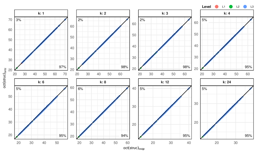
Figure 7: Comparison of nRMSE(%) between sntz and osqp non-negative forecast reconciliation using the oct($struc$) approach. The black line represents the bisector, where the nRMSE’s for oct($struc$)_osqp and oct($struc$)_sntz are equal. On the top-left (bottom-right) corner of each graph, the percentage of points above (below) the bisector is reported.

5.2 Forecast accuracy of the selected approaches

Table 6 shows the nRMSE(%) of the considered non-negative cross-temporal forecast reconciliation approaches, using the sntz heuristic, and the corresponding forecast skills over the benchmark forecasts PERS_bu. Overall, the accuracy improvements of the newly proposed approaches over the persistence model are in the range 16.5%–46.5%, whereas $3TIER_{bu}$ improvements are in the range 10.5%-38.3%. Partly bottom-up approaches, with cross-sectional reconciliation at the first step (i.e., ct$(wls_{cs},bu_{te})$ and ct$(struc_{cs},bu_{te})$) show a good performance for the six series at levels $\mathcal{L}_{0}$ and $\mathcal{L}_{1}$. For the 318 most disaggregated series at the bottom level, ct$(wlsv_{te},bu_{cs})$ and oct($wlsv$) rank first and second, respectively, and their accuracy indices are very close each other.

Table 6: Forecast accuracy of selected non-negative, cross-temporal reconciliation approaches and base forecasts in terms of nRMSE(%). Hourly and daily forecasts, forecast horizon: operating day. Bold entries and italic entries identify the best and the second best performing approaches, respectively.

	$\mathcal{L}_{0}$		$\mathcal{L}_{1}$		$\mathcal{L}_{2}$		$\mathcal{L}_{0}$		$\mathcal{L}_{1}$		$\mathcal{L}_{2}$
	H	D	H	D	H	D	H	D	H	D	H	D
	$nRMSE(\%)$						forecast skill
PERSbu	34.62	20.23	43.15	24.57	59.75	30.65	0.000	0.000	0.000	0.000	0.000	0.000
3TIERbu	26.03	12.48	33.95	16.75	53.46	25.19	0.248	0.383	0.213	0.318	0.105	0.178
oct$(struc)$	26.64	15.73	32.99	19.00	46.51	23.97	0.231	0.222	0.235	0.227	0.222	0.218
KA$(wlsv_{te},wls_{cs})$	23.59	13.55	30.23	16.91	44.48	22.21	0.319	0.330	0.299	0.312	0.256	0.275
ct$(struc_{cs},bu_{te})$	21.99	12.38	28.80	15.82	49.76	24.33	0.365	0.388	0.333	0.356	0.167	0.206
ct$(wls_{cs},bu_{te})$	21.23	10.82	28.97	15.01	49.88	23.66	0.387	0.465	0.329	0.389	0.165	0.228
ct$(struc_{te},bu_{cs})$	24.81	14.43	31.41	17.80	45.30	22.93	0.283	0.287	0.272	0.276	0.242	0.252
ct$(wlsv_{te},bu_{cs})$	23.50	13.42	30.13	16.78	44.42	22.12	0.321	0.337	0.302	0.317	0.257	0.278
oct$(wlsv)$	23.63	13.64	30.21	17.01	44.44	22.27	0.317	0.326	0.300	0.308	0.256	0.273
oct$(bdshr)$	24.13	13.92	30.45	17.12	45.24	22.54	0.303	0.312	0.294	0.303	0.243	0.265

From table 7, we see that even at distinct $\mathcal{L}_{1}$ series (Transmission Zones), the newly proposed approaches perform better than all the approaches considered by Yagli et al. [2019], as reported in table 4.

Table 7: Forecast accuracy of selected non-negative, cross-temporal reconciliation approaches and base forecasts in terms of nRMSE(%) for the series at $\mathcal{L}_{1}$ level. Hourly and daily forecasts, forecast horizon: operating day. Bold entries and italic entries identify the best and the second best performing approaches, respectively.

	TZ1		TZ2		TZ3		TZ4		TZ5
	H	D	H	D	H	D	H	D	H	D
	$nRMSE(\%)$
PERSbu	28.72	16.12	40.27	22.40	46.48	26.96	52.82	29.75	47.44	27.62
3TIERbu	22.81	10.43	33.34	16.72	34.01	17.06	46.40	22.80	33.16	16.75
oct$(struc)$	21.92	12.41	30.84	17.30	34.67	20.21	41.84	23.84	35.66	21.23
KA$(wlsv_{te},wls_{cs})$	20.23	11.10	28.57	15.43	30.98	17.45	39.72	22.09	31.64	18.51
ct$(struc_{cs},bu_{te})$	20.15	10.92	27.01	14.37	28.74	15.74	38.12	20.89	29.99	17.17
ct$(wls_{cs},bu_{te})$	19.33	9.72	28.11	14.18	29.55	15.10	39.20	20.17	28.68	15.88
ct$(struc_{te},bu_{cs})$	21.04	11.63	29.55	16.24	32.57	18.73	40.51	22.67	33.37	19.75
ct$(wlsv_{te},bu_{cs})$	20.20	10.98	28.53	15.35	30.89	17.37	39.69	22.01	31.32	18.19
oct$(wlsv)$	20.18	11.18	28.53	15.50	30.97	17.53	39.56	22.16	31.84	18.69
oct$(bdshr)$	21.00	11.74	29.25	16.02	31.63	17.85	39.73	22.27	30.65	17.74
	forecast skill
PERSbu	0	0	0	0	0	0	0	0	0	0
3TIERbu	0.206	0.353	0.172	0.254	0.268	0.367	0.121	0.234	0.301	0.394
oct$(struc)$	0.237	0.230	0.234	0.228	0.254	0.250	0.208	0.199	0.248	0.231
KA$(wlsv_{te},wls_{cs})$	0.296	0.312	0.291	0.311	0.334	0.353	0.248	0.258	0.333	0.330
ct$(struc_{cs},bu_{te})$	0.299	0.323	0.329	0.359	0.382	0.416	0.278	0.298	0.368	0.378
ct$(wls_{cs},bu_{te})$	0.327	0.397	0.302	0.367	0.364	0.440	0.258	0.322	0.396	0.425
ct$(struc_{te},bu_{cs})$	0.268	0.279	0.266	0.275	0.299	0.305	0.233	0.238	0.297	0.285
ct$(wlsv_{te},bu_{cs})$	0.297	0.319	0.292	0.315	0.335	0.356	0.249	0.260	0.340	0.341
oct$(wlsv)$	0.297	0.307	0.292	0.308	0.334	0.350	0.251	0.255	0.329	0.323
oct$(bdshr)$	0.269	0.272	0.274	0.285	0.320	0.338	0.248	0.251	0.354	0.358

In addition, almost all the new approaches significantly outperform $PERS_{bu}$, $3TIER_{bu}$, and oct$(struc)$ for both hourly and daily forecasts (figure 8).

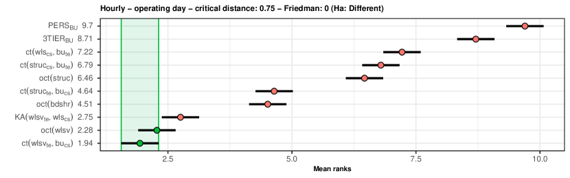
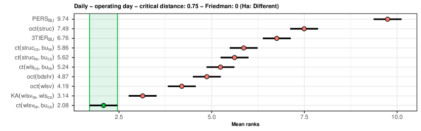
Figure 8: MCB-Nemenyi test on selected non-negative cross-temporal reconciliation approaches with operating day forecast horizon. $\mathcal{L}_{0},\mathcal{L}_{1},\mathcal{L}_{2}$ levels (324 series). Top panel: hourly forecasts; Bottom panel: daily forecasts. The mean rank of each approach is displayed to the right of their names. If the intervals of two forecast reconciliation approaches do not overlap, this indicates a statistically different performance. Thus, approaches that do not overlap with the green interval are considered significantly worse than the best, and vice-versa.

Finally, focusing on the two best performing approaches of the forecasting experiment (ct$(wlsv_{te},bu_{cs})$ and oct($wlsv)$), and looking at the nRMSEs of the individual series, it is worth noting that:

• ct$(wlsv_{te},bu_{cs})$ always produces more accurate forecasts than oct$(struc)$, for any series and granularity (figure 9),

• the accuracy increases of ct$(wlsv_{te},bu_{cs})$ over the NWP approach 3TIER_bu are still clear (figure 10), even though for daily forecasts 3TIER_bu performs better in about 1 case out 4;

• the accuracy of ct$(wlsv_{te},bu_{cs})$ and oct($wlsv)$ are practically indistinguishable (figure 11);

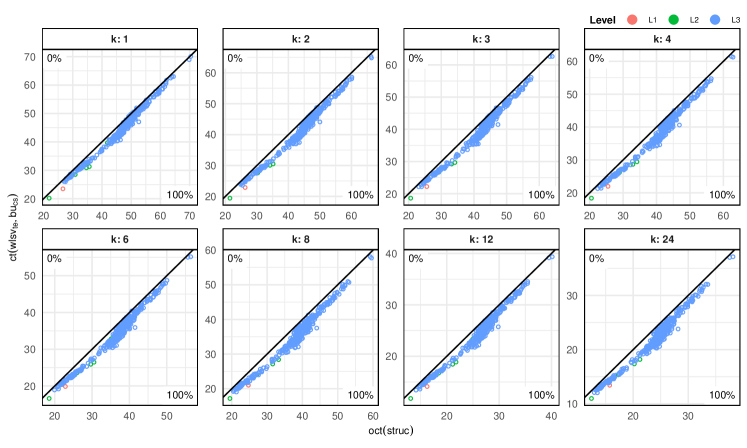
Figure 9: Comparison of nRMSE(%) between non-negative reconciliation approaches: oct$(struc)$ and ct$(wlsv_{te},bu_{cs})$, forecast horizon: operating day. The black line represents the bisector, where the nRMSE’s for both approaches are equal. On the top-left (bottom-right) corner of each graph, the percentage of points above (below) the bisector is reported.

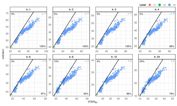
Figure 10: Comparison of nRMSE(%) between non-negative reconciliation approaches: $3TIER_{bu}$ and ct$(wlsv_{te},bu_{cs})$. Forecast horizon: operating day. The black line represents the bisector, where the nRMSE’s for both approaches are equal. On the top-left (bottom-right) corner of each graph, the percentage of points above (below) the bisector is reported.

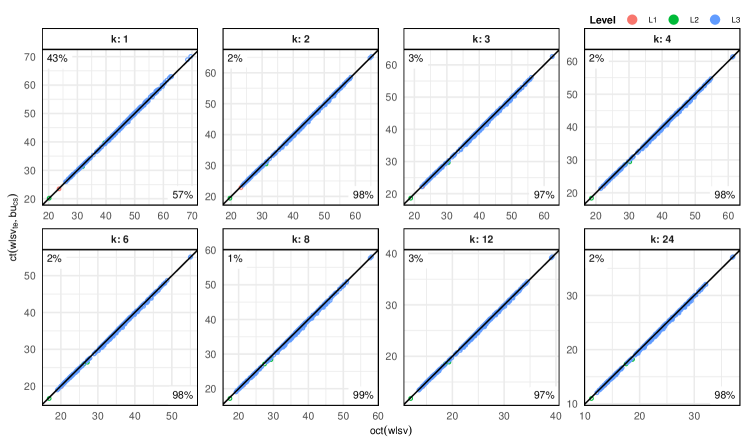
Figure 11: Comparison of nRMSE(%) between non-negative reconciliation approaches: oct$(wlsv)$ and ct$(wlsv_{te},bu_{cs})$, forecast horizon: operating day. The black line represents the bisector, where the nRMSE’s for both approaches are equal. On the top-left (bottom-right) corner of each graph, the percentage of points above (below) the bisector is reported.

We may thus conclude that, for the PV324 dataset considered in this work, a thorough exploitation of cross-temporal hierarchies significantly improves the forecasting accuracy as compared to the approaches considered in Yagli et al. [2019]. In particular, the use of the in-sample base forecast errors, even in the simple diagonal versions of te($wlsv$) (first step of ct($wlsv_{te},bu_{cs}$)), and oct($wlsv$), increases the forecasting accuracy at different time granularities.

6 Conclusion

Renewable energy is providing increasingly more energy to the grid all over the world. But grid operators must carefully manage the balance between the generation and consumption of energy to make the best use of abundant renewable energy. For an ISO, this provides greater grid stability, higher revenue and better use of what sun is available at any one time. Better short-term solar energy forecasts mean lower-emissions, cheaper energy and a more stable electricity grid. Solar forecasting is thus a key tool to achieve these results. In this paper, cross-temporal point forecast reconciliation has been applied to generate non-negative, fully coherent (both in space and time) forecasts of PV generated power. Both methodological and practical issues have been tackled, in order to develop effective and easy-to-handle cross-temporal forecasting approaches. Besides assuring both spatial and temporal coherence, and non-negativity of the reconciled forecasts, the results show that for the considered dataset, cross-temporal forecast reconciliation significantly improves on the sequential procedures proposed by Yagli et al. [2019], at any cross-sectional level of the hierarchy and for any temporal aggregation order. However, these findings should be considered neither conclusive, nor valid in general. Other forecasting experiments, through simulations and using other datasets, as well as in solar forecasting and in other application fields, should be performed to empirically robustify the results shown so far. In addition, other research queries could raise in the field of cross-temporal PV forecast reconciliation, like using reduced temporal hierarchies, as well as forecasting through appropriate Machine Learning end-to-end approaches (Stratigakos et al., 2022), and probabilistic instead of deterministic (point) forecasting (Panamtash and Zhou, 2018, Jeon et al., 2019, Panagiotelis et al., 2022, Yang, 2020a, Yang, 2020b, Ben Taieb et al., 2021). All these topics are left for future research.

Appendix A Cross-temporal bottom-up forecast reconciliation

A visual representation of cross-sectional, temporal, and cross-temporal bottom-up reconciliation is shown in figure 1, where the ‘bottom time series’ base forecasts are highlighted on a purple background, and the ‘upper time series’ bottom-up reconciled forecasts are highlighted on a pink background. The arrows show the direction(s) along with bottom-up reconciliation is performed. The deponent abbreviations ‘$cs$’, ‘$te$’, ‘$ct$’, are alternatively used to denote reconciled forecasts according to cross-sectional, temporal, and cross-temporal bottom-up, respectively.

(a) $\widetilde{\textbf{Y}}_{cs(bu)}$: cross-sectional bottom-up

(b) $\widetilde{\textbf{Y}}_{te\;bu}$: temporal bottom-up

(c) $\widetilde{\textbf{Y}}_{ct\;bu}$: cross-temporal bottom-up

Figure 1: A ‘visual’ representation of cross-sectional ($\widetilde{\textbf{Y}}_{cs(bu)}$), temporal ($\widetilde{\textbf{Y}}_{te(bu)}$), and cross-temporal ($\widetilde{\textbf{Y}}_{ct(bu)}$) bottom-up reconciled forecasts.

Cross-sectional bottom-up reconciliation of $k^{*}+m$ hierarchical time series’ base forecasts

The cross-sectional bottom-up ($cs(bu)$) reconciliation of hierarchical time series’ base forecasts at different temporal granularities (temporal aggregation levels) $k\in\mathcal{K}$, may be represented as follows:

$$\widetilde{\textbf{y}}_{\tau,cs(bu)}^{[k]}=\textbf{S}\widehat{\textbf{b}}_{\tau}^{[k]},\quad\tau=1,\ldots,\frac{m}{k},\quad k\in\mathcal{K}\quad\rightarrow\quad\widetilde{\textbf{Y}}_{cs(bu)}^{[k]}=\textbf{S}\widehat{\textbf{B}}^{[k]},\quad k\in\mathcal{K}.$$

In compact notation we have:

$$\widetilde{\textbf{Y}}_{cs(bu)}=\textbf{S}\widehat{\textbf{B}}\quad\rightarrow\quad\widetilde{\textbf{Y}}_{cs(bu)}^{\prime}=\widehat{\textbf{B}}^{\prime}\textbf{S}^{\prime}\quad\rightarrow\quad\widetilde{\textbf{y}}_{cs(bu)}=\left(\textbf{S}\otimes\textbf{I}_{k^{*}+m}\right)\widehat{\textbf{b}},$$

where $\widetilde{\textbf{y}}_{cs(bu)}=\text{vec}\left(\widetilde{\textbf{Y}}_{cs(bu)}^{\prime}\right)$, and $\widehat{\textbf{b}}=\text{vec}\left(\widehat{\textbf{B}}^{\prime}\right)$.

The $cs(bu)$ reconciled forecasts are obviously cross-sectionally coherent, but in general they are not temporally coherent:

$$\begin{array}[]{rcl}\textbf{U}^{\prime}\widetilde{\textbf{Y}}_{cs(bu)}=\textbf{0}_{[n_{a}\times(k^{*}+m)]}&\leftrightarrow&\left(\textbf{U}^{\prime}\otimes\textbf{I}_{k^{*}+m}\right)\widetilde{\textbf{y}}_{cs(bu)}=\textbf{0}_{[n_{a}(k^{*}+m)\times 1]}\\ \textbf{Z}^{\prime}\widetilde{\textbf{Y}}_{cs(bu)}^{\prime}\neq\textbf{0}_{[k^{*}\times n]}&\leftrightarrow&\left(\textbf{I}_{n}\otimes\textbf{Z}^{\prime}\right)\widetilde{\textbf{y}}_{cs(bu)}\neq\textbf{0}_{[k^{*}n\times 1]}\end{array}.$$

Temporal bottom-up reconciliation of $n$ individual time series’ base forecasts

The temporal bottom-up ($te(bu)$) reconciliation of $n$ individual time series’ base forecasts at different temporal granularities (temporal aggregation levels), may be represented as follows:

$$\begin{array}[]{c}\widetilde{\textbf{a}}_{i,te(bu)}=\textbf{R}\widehat{\textbf{a}}_{i}^{[1]},\quad i=1,\ldots,n_{a}\\ \widetilde{\textbf{b}}_{j,te(bu)}=\textbf{R}\widehat{\textbf{b}}_{j}^{[1]},\quad j=1,\ldots,n_{b}\\ \end{array}\quad\rightarrow\quad\begin{array}[]{c}\widetilde{\textbf{A}}_{te(bu)}=\textbf{R}\widehat{\textbf{A}}^{[1]\prime}\\ \widetilde{\textbf{B}}_{te(bu)}=\textbf{R}\widehat{\textbf{B}}^{[1]\prime}\\ \end{array}$$

and, finally,

$$\widetilde{\textbf{Y}}_{te(bu)}^{\prime}=\textbf{R}\widehat{\textbf{Y}}^{[1]\prime}\quad\rightarrow\quad\widetilde{\textbf{y}}_{te(bu)}=\left(\textbf{I}_{n}\otimes\textbf{R}\right)\widehat{\textbf{y}}^{[1]}.$$

The $te(bu)$ reconciled forecasts are obviously temporally coherent, but in general they are not cross-sectionally coherent:

$$\begin{array}[]{rcl}\textbf{Z}^{\prime}\widetilde{\textbf{Y}}_{te(bu)}^{\prime}=\textbf{0}_{[k^{*}\times n]}&\leftrightarrow&\left(\textbf{I}_{n}\otimes\textbf{Z}^{\prime}\right)\widetilde{\textbf{y}}_{te(bu)}=\textbf{0}_{[k^{*}n\times 1]}\\ \textbf{U}^{\prime}\widetilde{\textbf{Y}}_{te(bu)}\neq\textbf{0}_{[n_{a}\times(k^{*}+m)]}&\leftrightarrow&\left(\textbf{U}^{\prime}\otimes\textbf{I}_{k^{*}+m}\right)\widetilde{\textbf{y}}_{te(bu)}\neq\textbf{0}_{[n_{a}(k^{*}+m)\times 1]}\end{array}.$$

Cross-temporal bottom-up reconciliation of $n$ individual time series’ base forecasts for different temporal granularities

The cross-temporal bottom-up ($ct(bu)$) reconciliation of $k^{*}+m$ hierarchical time series’ base forecasts at different temporal granularities, may be represented as follows:

$$\text{vec}\left(\widetilde{\textbf{Y}}_{ct(bu)}^{\prime}\right)=\left(\textbf{S}\otimes\textbf{R}\right)\text{vec}\left(\widehat{\textbf{B}}^{[1]\prime}\right)\quad\leftrightarrow\quad\widetilde{\textbf{y}}_{cs(bu)}\left(\textbf{S}\otimes\textbf{R}\right)\widehat{\textbf{b}}^{[1]},$$ (8)

where $\widehat{\textbf{b}}^{[1]}=\text{vec}\left(\widehat{\textbf{B}}^{[1]\prime}\right)$. Let us consider now the coherency checks for the $ct(bu)$ reconciled forecasts:

• cross-sectional coherency

  $$\left(\textbf{U}^{\prime}\otimes\textbf{I}_{k^{*}+m}\right)\left(\textbf{S}\otimes\textbf{R}\right)\widehat{\textbf{b}}^{[1]}=\left(\textbf{U}^{\prime}\textbf{S}\otimes\textbf{R}\right)\widehat{\textbf{b}}^{[1]}=\textbf{0}_{[n_{a}(k^{*}+m)\times 1]},$$

  since $\textbf{U}^{\prime}\textbf{S}=\left[\textbf{I}_{n_{a}}\;-\textbf{C}\right]\left[\begin{array}[]{c}\textbf{C}\\ \textbf{I}_{n_{b}}\end{array}\right]=\textbf{C}-\textbf{C}=\textbf{0}_{[n_{a}\times n_{b}]}$;

• temporal coherency

  $$\left(\textbf{I}_{n}\otimes\textbf{Z}^{\prime}\right)\left(\textbf{S}\otimes\textbf{R}\right)\widehat{\textbf{b}}^{[1]}=\left(\textbf{S}\otimes\textbf{Z}^{\prime}\textbf{R}\right)\widehat{\textbf{b}}^{[1]}=\textbf{0}_{[k^{*}n\times 1]},$$

  since $\textbf{Z}^{\prime}\textbf{R}=\left[\textbf{I}_{k^{*}}\;-\textbf{K}\right]\left[\begin{array}[]{c}\textbf{K}\\ \textbf{I}_{m}\end{array}\right]=\textbf{K}-\textbf{K}=\textbf{0}_{[k^{*}\times m]}$.

In the end, cross temporal bottom-up reconciliation can be tought of as a two-step sequential cross temporal reconciliation approach, where either cross-sectional reconciliation of the high-frequency bottom time series base forecasts (the ‘very’ bottom series of a cross-temporal hierarchy), is followed by temporal reconciliation, or vice-versa. For, looking at expression (8), and by exploiting the properties of the vec operator (Harville, 2008, p. 345), it is:

$$\left(\textbf{S}\otimes\textbf{R}\right)\text{vec}\left(\widehat{\textbf{B}}^{[1]\prime}\right)=\text{vec}\left[\textbf{R}\left(\widehat{\textbf{B}}^{[1]\prime}\right)\textbf{S}^{\prime}\right],$$

which may be interpretated in two different, equivalent ways:

• looking at the expression $\textbf{R}\left(\widehat{\textbf{B}}^{[1]\prime}\right)\textbf{S}^{\prime}$ from the right, one first computes the cross-sectional bottom-up reconciled forecasts of all the $n$ high-frequency time series, $\widetilde{\textbf{Y}}_{cs(bu)}^{[1]}=\textbf{S}\widehat{\textbf{B}}^{[1]}$. These forecasts, that are not temporally coherent with the base forecasts of the same series at lower temporal granularity (i.e., $\widehat{\textbf{Y}}^{[k]}$, $k\neq 1$), are then reconciled via temporal bottom-up, $\widetilde{\textbf{Y}}_{ct(bu)}^{\prime}=\textbf{R}\widetilde{\textbf{Y}}_{cs(bu)}^{[1]\prime}$:

  $$\widehat{\textbf{B}}^{[1]}\quad\xrightarrow{\quad cs(bu)\quad}\quad\widetilde{\textbf{Y}}_{cs(bu)}^{[1]}\quad\xrightarrow{\quad te(bu)\quad}\quad\widetilde{\textbf{Y}}_{ct(bu)};$$

• moving in turn from the left, one first computes the temporally reconciled forecasts of the $n_{b}$ bottom time series of the hierarchy, $\widetilde{\textbf{B}}_{te(bu)}^{\prime}=\textbf{R}\left(\widehat{\textbf{B}}^{[1]\prime}\right)$. These forecasts, that are not cross-sectionally coherent with the base forecasts of the $n_{a}$ upper time series of the hierarchy, are then reconciled via cross-sectional bottom-up, $\widetilde{\textbf{Y}}_{ct(bu)}=\textbf{S}\left(\widetilde{\textbf{B}}_{te(bu)}\right)$:

  $$\widehat{\textbf{B}}^{[1]}\quad\xrightarrow{\quad te(bu)\quad}\quad\widetilde{\textbf{B}}_{te(bu)}\quad\xrightarrow{\quad cs(bu)\quad}\quad\widetilde{\textbf{Y}}_{ct(bu)}.$$

The two equivalent interpretations of the cross-temporal bottom-up approach are represented in Figure 2, where $\widetilde{\textbf{B}}_{ct(bu)}^{[1]}\equiv\widehat{\textbf{B}}^{[1]}$, $\widetilde{\textbf{A}}_{ct(bu)}^{[1]}\equiv\widetilde{\textbf{A}}_{cs(bu)}^{[1]}$, and $\widetilde{\textbf{B}}_{ct(bu)}^{[k]}\equiv\widetilde{\textbf{B}}_{te(bu)}^{[k]}$, $k>1$.

(a) $cs(bu)$ on $\widehat{\textbf{Y}}^{[1]}$ $+$ $te(bu)$ on $\widetilde{\textbf{Y}}_{cs(bu)}$.

(b) $te(bu)$ on $\widehat{\textbf{B}}^{[1]}$ $+$ $cs(bu)$ on $\widetilde{\textbf{B}}_{te(bu)}$.

Figure 2: A ‘visual’ interpretation of $\widetilde{\textbf{Y}}_{ct(bu)}$ in two different, equivalent ways.

Appendix B Proof of the theorem 1

1. Let $\textbf{U}^{\prime}_{n_{a}\times n}$ and $\textbf{Z}^{\prime}_{m\times(k^{\ast}+m)}$ be the cross-sectional and temporal, respectively, zero constraints kernel matrix. Let

   $$\textbf{M}_{cs}^{[k]}=\textbf{M}_{cs}=\left[\textbf{I}_{n}-\textbf{W}\textbf{U}\left(\textbf{U}^{\prime}\textbf{W}\textbf{U}\right)^{-1}\textbf{U}^{\prime}\right],\quad k\in\mathcal{K}$$

   and

   $$\textbf{M}_{te,i}=\textbf{M}_{te}=\left[\textbf{I}_{k^{\ast}+m}-\bm{\mathsf{\Omega}}\textbf{Z}\left(\textbf{Z}^{\prime}\bm{\mathsf{\Omega}}\textbf{Z}\right)^{-1}\textbf{Z}^{\prime}\right],\quad i=1,\ldots,n,$$

   be the cross-sectional and temporal projection matrices, respectively, such that:

   $$\begin{array}[]{rcll}\widetilde{\textbf{Y}}_{cs}^{[k]}&=&\textbf{M}_{cs}\widehat{\textbf{Y}}^{[k]},&k\in\mathcal{K},\\ \widetilde{\textbf{y}}_{te,i}&=&\textbf{M}_{te}\widehat{\textbf{y}}_{i},&i=1,\ldots,n,\end{array}$$

   where $\widehat{\textbf{Y}}^{[k]}$ and $\widetilde{\textbf{Y}}_{cs}^{[k]}$ are the $\left(n\times\frac{m}{k}\right)$ matrices with, respectively, the base and the cross-sectional reconciled forecasts of the $n$ series at time granularity $k$, and $\widehat{\textbf{y}}_{i}$ and $\widetilde{\textbf{y}}_{te,i}$ are the $\left[(k^{*}+m)\times 1\right]$ vectors with, respectively, the base and the temporal reconciled forecasts at all time granularities for the $i$-th series. In compact matrix form we get:

   $$\begin{array}[]{rcl}\widetilde{\textbf{Y}}_{cs}&=&\left[\widetilde{\textbf{Y}}_{cs}^{[m]}\;\widetilde{\textbf{Y}}_{cs}^{[k_{p-1}]}\ldots\widetilde{\textbf{Y}}_{cs}^{[k_{2}]}\;\widetilde{\textbf{Y}}_{cs}^{[1]}\right]=\textbf{M}_{cs}\left[\widehat{\textbf{Y}}^{[m]}\;\widehat{\textbf{Y}}^{[k_{p-1}]}\ldots\widehat{\textbf{Y}}^{[k_{2}]}\;\widehat{\textbf{Y}}^{[1]}\right]=\textbf{M}_{cs}\widehat{\textbf{Y}},\\ \widetilde{\textbf{Y}}_{te}&=&\left\{\textbf{M}_{te}\left[\widehat{\textbf{y}}_{1}\ldots\widehat{\textbf{y}}_{i}\ldots\widehat{\textbf{y}}_{n}\right]\right\}^{\prime}=\left\{\textbf{M}_{te}\widehat{\textbf{Y}}^{\prime}\right\}^{\prime}.\end{array}$$

   Then, $\widetilde{\textbf{Y}}_{cst}$ is obtained by first operating a cross-sectional reconciliation (step 1, $\widetilde{\textbf{Y}}_{cs}$), and then reconciling via temporal hierarchies the forecasts obtained in the previous step (step 2, $\widetilde{\textbf{Y}}_{cst}$). In matrix terms:

   $$\begin{array}[]{rcl}\text{step 1 }&\widetilde{\textbf{Y}}_{cs}&=\textbf{M}_{cs}\widehat{\textbf{Y}}\\ \text{step 2 }&\widetilde{\textbf{Y}}_{cst}&=\left\{\textbf{M}_{te}\widetilde{\textbf{Y}}_{cs}^{\prime}\right\}^{\prime}=\widetilde{\textbf{Y}}_{cs}\textbf{M}_{te}^{\prime}=\textbf{M}_{cs}\widehat{\textbf{Y}}\textbf{M}_{te}^{\prime}\end{array}$$

   where $\widehat{\textbf{Y}}$ is the ($n\times(k^{\ast}+m)$) base forecasts matrix. Viceversa, $\widetilde{\textbf{Y}}_{tcs}$ is obtained by first operating a temporal reconciliation (step 1, $\widetilde{\textbf{Y}}_{te}$), and finally a cross-sectional reconciliation is applied (step 2):

   $$\begin{array}[]{rcl}\text{step 1 }&\widetilde{\textbf{Y}}_{te}&=\left\{\textbf{M}_{te}\widehat{\textbf{Y}}^{\prime}\right\}^{\prime}=\widehat{\textbf{Y}}\textbf{M}_{te}^{\prime}\\ \text{step 2 }&\widetilde{\textbf{Y}}_{tcs}&=\textbf{M}_{cs}\widetilde{\textbf{Y}}_{te}=\textbf{M}_{cs}\widehat{\textbf{Y}}\textbf{M}_{te}^{\prime}=\widetilde{\textbf{Y}}_{cst}.\end{array}$$

   The forecasts $\widetilde{\textbf{Y}}_{tcs}$ (and $\widetilde{\textbf{Y}}_{cst}$) (a single two-step iteration) are cross-temporally reconciled because:

   $$\textbf{U}^{\prime}\widetilde{\textbf{Y}}_{tcs} =\textbf{U}^{\prime}\textbf{M}_{cs}\widehat{\textbf{Y}}\textbf{M}_{te}^{\prime}=\left[\textbf{U}^{\prime}-\textbf{U}^{\prime}\textbf{W}\textbf{U}\left(\textbf{U}^{\prime}\textbf{W}\textbf{U}\right)^{-1}\textbf{U}^{\prime}\right]\widehat{\textbf{Y}}\textbf{M}_{te}^{\prime}=\left[\textbf{U}^{\prime}-\textbf{U}^{\prime}\right]\widehat{\textbf{Y}}\textbf{M}_{te}^{\prime}=\textbf{0}_{n_{a}\times(k^{\ast}+m)}$$

   and

   $$\textbf{Z}^{\prime}\widetilde{\textbf{Y}}_{tcs}^{\prime} =\textbf{Z}^{\prime}\textbf{M}_{te}\widehat{\textbf{Y}}^{\prime}\textbf{M}_{cs}^{\prime}=\left[\textbf{Z}^{\prime}-\textbf{Z}^{\prime}\bm{\mathsf{\Omega}}\textbf{Z}\left(\textbf{Z}^{\prime}\bm{\mathsf{\Omega}}\textbf{Z}\right)^{-1}\textbf{Z}^{\prime}\right]\textbf{M}_{cs}^{\prime}=\left[\textbf{Z}^{\prime}-\textbf{Z}^{\prime}\right]\widehat{\textbf{Y}}^{\prime}\textbf{M}_{cs}^{\prime}=\textbf{0}_{m\times n}.$$

2. Using matrix vectorization and structural representation for the cross-temporal reconciliation problem we have:

   $$\begin{aligned} \widetilde{\textbf{y}}_{oct}=\textbf{F}\left(\textbf{F}^{\prime}\bm{\mathsf{\Omega}}_{ct}^{-1}\textbf{F}\right)^{-1}\textbf{F}^{\prime}\widehat{\textbf{y}}\end{aligned},$$

   where $\widetilde{\textbf{y}}_{oct}=\mathrm{vec}\left(\widetilde{\textbf{Y}}_{oct}^{\prime}\right)$, $\widehat{\textbf{y}}=\mathrm{vec}\left(\widehat{\textbf{Y}}_{oct}^{\prime}\right)$, and $\textbf{F}=\textbf{S}\otimes\textbf{R}$ is the [$n(k^{\ast}+m)\times mn_{b}$] cross-temporal summing matrix. Let $\bm{\mathsf{\Omega}}_{ct}=\textbf{W}\otimes\bm{\mathsf{\Omega}}$ be the cross-temporal error covariance matrix, by exploiting the properties of the Kronecker product (Henderson and Searle, 1981; Harville, 2008), we obtain:

   $$\widetilde{\textbf{y}}_{oct} =\textbf{F}\left(\textbf{F}^{\prime}\bm{\mathsf{\Omega}}_{ct}^{-1}\textbf{F}\right)^{-1}\textbf{F}^{\prime}\bm{\mathsf{\Omega}}_{ct}^{-1}\widehat{\textbf{y}}$$

   $$=(\textbf{S}\otimes\textbf{R})\left[(\textbf{S}\otimes\textbf{R})^{\prime}(\textbf{W}\otimes\bm{\mathsf{\Omega}})^{-1}(\textbf{S}\otimes\textbf{R})\right]^{-1}(\textbf{S}\otimes\textbf{R})^{\prime}(\textbf{W}\otimes\bm{\mathsf{\Omega}})^{-1}\widehat{\textbf{y}}$$

   $$=(\textbf{S}\otimes\textbf{R})\left[(\textbf{S}^{\prime}\otimes\textbf{R}^{\prime})(\textbf{W}^{-1}\otimes\bm{\mathsf{\Omega}}^{-1})(\textbf{S}\otimes\textbf{R})\right]^{-1}(\textbf{S}^{\prime}\otimes\textbf{R}^{\prime})(\textbf{W}^{-1}\otimes\bm{\mathsf{\Omega}}^{-1})\widehat{\textbf{y}}$$

   $$=(\textbf{S}\otimes\textbf{R})\left(\textbf{S}^{\prime}\textbf{W}^{-1}\textbf{S}\otimes\textbf{R}^{\prime}\bm{\mathsf{\Omega}}^{-1}\textbf{R}\right)^{-1}(\textbf{S}^{\prime}\textbf{W}^{-1}\otimes\textbf{R}^{\prime}\bm{\mathsf{\Omega}}^{-1})\widehat{\textbf{y}}$$

   $$=\left[\textbf{S}\left(\textbf{S}^{\prime}\textbf{W}^{-1}\textbf{S}\right)^{-1}\textbf{S}^{\prime}\textbf{W}^{-1}\otimes\textbf{R}\left(\textbf{R}^{\prime}\bm{\mathsf{\Omega}}^{-1}\textbf{R}\right)^{-1}\textbf{R}^{\prime}\bm{\mathsf{\Omega}}^{-1}\right]\widehat{\textbf{y}}.$$

   Exploiting the structural notation also in the temporal then cross-sectional iterative procedure and the vectorization $\widetilde{\textbf{y}}_{tcs}=\mathrm{vec}\left(\widehat{\textbf{Y}}_{tcs}^{\prime}\right)$, we obtain:

   $$\widetilde{\textbf{y}}_{tcs} =\textbf{P}\left[\textbf{I}_{k^{\ast}+m}\otimes\textbf{S}\left(\textbf{S}^{\prime}\textbf{W}^{-1}\textbf{S}\right)^{-1}\textbf{S}^{\prime}\textbf{W}^{-1}\right]\textbf{P}^{\prime}\left[\textbf{I}_{n}\otimes\textbf{R}\left(\textbf{R}^{\prime}\bm{\mathsf{\Omega}}^{-1}\textbf{R}\right)^{-1}\textbf{R}^{\prime}\bm{\mathsf{\Omega}}^{-1}\right]\widehat{\textbf{y}}$$

   $$=\left[\textbf{S}\left(\textbf{S}^{\prime}\textbf{W}^{-1}\textbf{S}\right)^{-1}\textbf{S}^{\prime}\textbf{W}^{-1}\otimes\textbf{I}_{k^{\ast}+m}\right]\left[\textbf{I}_{n}\otimes\textbf{R}\left(\textbf{R}^{\prime}\bm{\mathsf{\Omega}}^{-1}\textbf{R}\right)^{-1}\textbf{R}^{\prime}\bm{\mathsf{\Omega}}^{-1}\right]\widehat{\textbf{y}}$$

   $$=\left[\textbf{S}\left(\textbf{S}^{\prime}\textbf{W}^{-1}\textbf{S}\right)^{-1}\textbf{S}^{\prime}\textbf{W}^{-1}\otimes\textbf{R}\left(\textbf{R}^{\prime}\bm{\mathsf{\Omega}}^{-1}\textbf{R}\right)^{-1}\textbf{R}^{\prime}\bm{\mathsf{\Omega}}^{-1}\right]\widehat{\textbf{y}}=\widetilde{\textbf{y}}_{oct}.$$

   Finally, $\widetilde{\textbf{Y}}_{tcs}=\widetilde{\textbf{Y}}_{oct}$ and, following from point 1, $\widetilde{\textbf{Y}}_{tcs}=\widetilde{\textbf{Y}}_{cst}=\widetilde{\textbf{Y}}_{oct}$.

$\Box$

The heuristic KA with constant cross-sectional and temporal error covariance matrices

In the Kourentzes and Athanasopoulos [2019] approach (section 2.5), the temporally reconciled predictions at step 1, $\widehat{\textbf{Y}}\textbf{M}_{te}^{\prime}$, are cross-sectionally reconciled via premultiplication by the matrix $\overline{\textbf{M}}=\frac{1}{p}\sum_{k\in\mathcal{K}}\textbf{M}^{[k]}_{cs}$. As $\textbf{W}^{[k]}=\textbf{W}$, $k\in\mathcal{K}$, $\textbf{M}^{[k]}_{cs}=\textbf{M}_{cs}$, and $\overline{\textbf{M}}=\textbf{M}_{cs}$. Then,

$$\widetilde{\textbf{Y}}_{KA}=\overline{\textbf{M}}\widehat{\textbf{Y}}\textbf{M}_{te}^{\prime}=\textbf{M}_{cs}\widehat{\textbf{Y}}\textbf{M}_{te}^{\prime}=\widetilde{\textbf{Y}}_{cst}=\widetilde{\textbf{Y}}_{tcs}.$$

Acknowldgements

Parts of this research were carried in the frame of the PRIN2017 project “HiDEA: Advanced Econometrics for High-frequency Data”, 2017RSMPZZ.

On-line appendix: supplementary tables and graphs

Table OA.1: Number of series with at least one negative reconciled forecast. All temporal aggregation orders, forecast horizon: operating day.

k	comb	n	min	max	fmin	fmax
1	base	350	4	6	-15.617	0.000
1	oct($ols$)	350	109	324	-69.165	0.000
1	ite($struc_{cs},ols_{te}$)	350	137	324	-20.739	0.000
1	ite($ols_{cs},struc_{te}$)	350	91	324	-17.961	0.000
1	oct($struc$)	350	89	324	-14.292	0.000
1	te($ols_{2}$)+cs($ols$)	350	42	324	-12.993	0.000
1	te($struc_{2}$)+cs($ols$)	350	36	324	-12.994	0.000
1	te($ols_{2}$)+cs($struc$)	350	144	324	-7.526	0.000
1	te($struc_{2}$)+cs($struc$)	350	124	324	-7.642	0.000
2	base	350	171	320	-32.639	0
2	oct($ols$)	350	60	324	-32.147	0
2	ite($struc_{cs},ols_{te}$)	350	56	324	-31.867	0
2	ite($ols_{cs},struc_{te}$)	350	26	324	-18.728	0
2	oct($struc$)	350	33	324	-22.719	0
2	te($ols_{2}$)+cs($ols$)	350	29	324	-27.023	0
2	te($struc_{2}$)+cs($ols$)	350	24	324	-27.025	0
2	te($ols_{2}$)+cs($struc$)	350	82	321	-20.451	0
2	te($struc_{2}$)+cs($struc$)	350	58	322	-17.812	0
3	base	350	60	323	-45.120	0
3	oct($ols$)	350	6	324	-31.640	0
3	ite($struc_{cs},ols_{te}$)	350	9	324	-35.059	0
3	ite($ols_{cs},struc_{te}$)	350	20	324	-28.085	0
3	oct($struc$)	350	27	323	-32.377	0
3	te($ols_{2}$)+cs($ols$)	350	3	324	-43.853	0
3	te($struc_{2}$)+cs($ols$)	350	1	324	-43.855	0
3	te($ols_{2}$)+cs($struc$)	350	40	324	-42.255	0
3	te($struc_{2}$)+cs($struc$)	350	18	324	-42.445	0
4	base	350	14	321	-88.776	0
4	oct($ols$)	350	11	322	-42.291	0
4	ite($ols_{cs},struc_{te}$)	350	15	322	-35.129	0
4	ite($struc_{cs},ols_{te}$)	350	25	318	-44.256	0
4	oct($struc$)	350	14	324	-40.562	0
4	te($ols_{2}$)+cs($ols$)	350	2	324	-85.947	0
4	te($struc_{2}$)+cs($ols$)	350	1	324	-85.956	0
4	te($ols_{2}$)+cs($struc$)	350	2	324	-63.026	0
4	te($struc_{2}$)+cs($struc$)	350	1	324	-63.927	0
6	base	350	19	321	-146.702	0
6	oct($ols$)	350	3	324	-61.415	0
6	ite($struc_{cs},ols_{te}$)	350	4	323	-67.327	0
6	ite($ols_{cs},struc_{te}$)	350	17	323	-53.857	0
6	oct($struc$)	350	16	322	-63.281	0
6	te($ols_{2}$)+cs($ols$)	347	0	324	-133.572	0
6	te($struc_{2}$)+cs($ols$)	347	0	324	-133.571	0
6	te($ols_{2}$)+cs($struc$)	347	0	324	-89.955	0
6	te($struc_{2}$)+cs($struc$)	349	0	324	-88.924	0
8	base	212	0	238	-866.818	0.000
8	oct($ols$)	300	0	305	-78.762	0.000
8	oct($struc$)	276	0	324	-51.806	0.000
8	ite($struc_{cs},ols_{te}$)	296	0	272	-53.688	0.000
8	ite($ols_{cs},struc_{te}$)	274	0	319	-42.734	0.000
8	te($ols_{2}$)+cs($ols$)	307	0	320	-680.766	0.000
8	te($struc_{2}$)+cs($ols$)	285	0	324	-680.488	0.000
8	te($ols_{2}$)+cs($struc$)	300	0	241	-56.011	0.000
8	te($struc_{2}$)+cs($struc$)	284	0	268	-52.341	0.000
12	base	46	0	57	-59.405	-0.001
12	oct($ols$)	14	0	78	-15.328	-0.001
12	ite($struc_{cs},ols_{te}$)	13	0	45	-7.949	-0.004
12	ite($ols_{cs},struc_{te}$)	8	0	31	-6.672	-0.001
12	oct($struc$)	6	0	18	-0.537	-0.009
12	te($ols_{2}$)+cs($ols$)	35	0	95	-32.259	0.000
12	te($struc_{2}$)+cs($ols$)	26	0	100	-32.191	0.000
12	te($ols_{2}$)+cs($struc$)	19	0	75	-9.799	0.000
12	te($struc_{2}$)+cs($struc$)	12	0	69	-6.544	-0.002
24	base	11	0	35	-51.205	-0.006
24	oct($ols$)	11	0	60	-29.615	-0.001
24	ite($struc_{cs},ols_{te}$)	11	0	33	-10.363	0.000
24	ite($ols_{cs},struc_{te}$)	6	0	28	-8.915	-0.008
24	oct($struc$)	4	0	11	-1.020	-0.026
24	te($ols_{2}$)+cs($ols$)	10	0	72	-15.037	-0.018
24	te($struc_{2}$)+cs($ols$)	10	0	71	-14.791	-0.005
24	te($ols_{2}$)+cs($struc$)	10	0	43	-12.969	-0.005
24	te($struc_{2}$)+cs($struc$)	5	0	31	-7.042	-0.002

A general overview of the accuracy of the considered procedures at any tempural granularity is given by table LABEL:table_Yagli_original_appendix, while a visual confirmation of the performance of ct-struc is shown by the MCB graphs in figure 5 in the main paper. The ct-struc daily reconciled forecasts show the best performance, significantly different from all the other procedures, while at hourly level it ranks second, the best being t-struc₂ + cs-struc. However, t-struc₂ + cs-struc produces temporally incoherent forecasts, and a punctual assessment of the performance of these two procedures in terms of nRMSE (figure LABEL:fig:comparison_ct-struc_vs_tcs-struc2-struc) confirms that their forecasting accuracy is about the same.

$\mathcal{L}$	comb	1	2	3	4	6	8	12	24
1	PERSbu	34.62	34.14	33.35	33.11	29.45	32.23	20.83	20.23
1	3TIERbu	26.03	25.34	24.56	23.31	22.09	19.89	15.70	12.48
1	base	27.85	27.55	28.31	29.69	28.01	35.32	21.04	18.17
1	oct($ols$)	30.69	29.96	28.29	28.86	25.26	28.12	18.39	17.91
1	ite($struc_{cs},ols_{te}$)	28.74	28.25	27.14	27.38	24.34	26.64	17.82	17.33
1	ite($ols_{cs},struc_{te}$)	28.26	27.84	27.09	27.00	24.17	26.24	17.46	16.96
1	oct($struc$)	26.71	26.35	25.67	25.57	23.03	24.80	16.74	16.24
1	te($ols_{2}$)+cs($ols$)	27.80	27.41	27.91	29.38	27.39	34.11	20.80	17.96
1	te($struc_{2}$)+cs($ols$)	27.80	27.41	27.90	29.37	27.39	34.10	20.80	17.95
1	te($ols_{2}$)+cs($struc$)	27.02	26.73	26.73	27.75	25.13	28.93	19.11	17.24
1	te($struc_{2}$)+cs($struc$)	26.17	25.86	25.83	26.80	24.37	27.95	18.58	16.68
2	PERSbu	43.15	42.42	41.27	40.81	36.29	39.19	25.66	24.57
2	3TIERbu	33.95	32.94	31.90	30.62	28.02	26.99	19.87	16.75
2	base	34.24	34.04	33.79	35.01	33.11	40.51	25.16	20.94
2	oct($ols$)	39.17	37.97	35.24	36.12	31.27	34.80	22.58	21.74
2	ite($struc_{cs},ols_{te}$)	35.48	34.74	33.24	33.44	29.65	32.16	21.66	20.82
2	ite($ols_{cs},struc_{te}$)	35.19	34.57	33.48	33.28	29.74	31.95	21.47	20.61
2	oct($struc$)	33.11	32.54	31.60	31.37	28.19	30.06	20.49	19.64
2	te($ols_{2}$)+cs($ols$)	34.36	34.52	35.40	36.29	35.64	45.42	26.24	21.80
2	te($struc_{2}$)+cs($ols$)	34.34	34.50	35.38	36.26	35.62	45.40	26.23	21.79
2	te($ols_{2}$)+cs($struc$)	33.40	33.07	32.82	33.64	30.70	35.26	23.20	20.62
2	te($struc_{2}$)+cs($struc$)	32.44	32.07	31.80	32.54	29.81	34.14	22.59	19.96
3	PERSbu	59.75	56.81	54.23	52.87	46.82	49.07	33.12	30.65
3	3TIERbu	53.46	50.57	48.33	46.19	41.36	40.72	29.28	25.19
3	base	53.46	47.22	44.87	44.30	39.68	42.66	30.92	25.82
3	oct($ols$)	51.54	48.48	45.06	45.17	39.41	42.39	28.50	26.73
3	ite($struc_{cs},ols_{te}$)	49.32	46.47	43.80	43.45	38.38	40.64	27.92	26.14
3	ite($ols_{cs},struc_{te}$)	48.20	45.50	43.45	42.51	37.83	39.64	27.28	25.46
3	oct($struc$)	46.74	44.02	42.05	41.07	36.67	38.16	26.56	24.73
3	te($ols_{2}$)+cs($ols$)	48.52	46.20	45.02	45.58	42.49	50.21	31.50	26.71
3	te($struc_{2}$)+cs($ols$)	47.77	45.52	44.64	44.96	42.07	49.67	31.19	26.36
3	te($ols_{2}$)+cs($struc$)	47.76	45.19	43.49	43.72	39.27	43.19	29.26	25.98
3	te($struc_{2}$)+cs($struc$)	46.25	43.69	42.24	42.12	38.05	41.53	28.38	25.03

References

- 3TIER [2010] 3TIER, 2010. Development of Regional Wind Resource and Wind Plant Output Datasets: Final Subcontract Report. Electricity generation, Energy storage, Forecasting wind, Solar energy, Wind energy, Wind farms, Wind modeling. URL: https://digitalscholarship.unlv.edu/renew_pubs/4. (visited on May 10, 2022).
- Athanasopoulos et al. [2009] Athanasopoulos, G., Ahmed, R.A., Hyndman, R.J., 2009. Hierarchical forecasts for Australian domestic tourism. International Journal of Forecasting 25, 146–166. doi:10.1016/j.ijforecast.2008.07.004.
- Athanasopoulos et al. [2017] Athanasopoulos, G., Hyndman, R.J., Kourentzes, N., Petropoulos, F., 2017. Forecasting with temporal hierarchies. European Journal of Operational Research 262, 60–74. doi:10.1016/j.ejor.2017.02.046.
- Babai et al. [2022] Babai, M.Z., Boylan, J.E., Rostami-Tabar, B., 2022. Demand forecasting in supply chains: a review of aggregation and hierarchical approaches. International Journal of Production Research 60, 324–348. doi:10.1080/00207543.2021.2005268.
- Bates et al. [2022] Bates, D., Maechler, M., Jagan, M., Davis, T.A., Oehlschlägel, J., Riedy, J., 2022. Package Matrix: Sparse and Dense Matrix Classes and Methods. Version 1.4-1. URL: https://cran.r-project.org/web/packages/Matrix/index.html.
- Ben Taieb et al. [2021] Ben Taieb, S., Taylor, J.W., Hyndman, R.J., 2021. Hierarchical Probabilistic Forecasting of Electricity Demand with Smart Meter Data. Journal of the American Statistical Association 116, 27–43. doi:https://doi.org/10.1080/01621459.2020.1736081.
- Byron [1978] Byron, R.P., 1978. The Estimation of Large Social Account Matrices. Journal of the Royal Statistical Society. Series A 141, 359–367. doi:10.2307/2344807.
- Dangerfield and Morris [1992] Dangerfield, B., Morris, J., 1992. Top-down or bottom-up: Aggregate versus disaggregate extrapolations. International Journal of Forecasting 6, 233–241. doi:10.1016/0169-2070(92)90121-O.
- Davis [2006] Davis, T.A., 2006. Direct Methods for Sparse Linear Systems. Society for Industrial and Applied Mathematics.