Machine learning based modeling of disordered elemental semiconductors: understanding the atomic structure of a-Si and a-C

Abstract

Disordered elemental semiconductors, most notably a-C and a-Si, are ubiquitous in a myriad of different applications. These exploit their unique mechanical and electronic properties. In the past couple of decades, density functional theory (DFT) and other quantum mechanics-based computational simulation techniques have been successful at delivering a detailed understanding of the atomic and electronic structure of crystalline semiconductors. Unfortunately, the complex structure of disordered semiconductors sets the time and length scales required for DFT simulation of these materials out of reach. In recent years, machine learning (ML) approaches to atomistic modeling have been developed that provide an accurate approximation of the DFT potential energy surface for a small fraction of the computational time. These ML approaches have now reached maturity and are starting to deliver the first conclusive insights into some of the missing details surrounding the intricate atomic structure of disordered semiconductors. In this Topical Review we give a brief introduction to ML atomistic modeling and its application to amorphous semiconductors. We then take a look at how ML simulations have been used to improve our current understanding of the atomic structure of a-C and a-Si.

I Introduction

Since the inception of the first experimental semiconductor diodes in the early 1900s the presence of semiconductors in daily appliances as well as high-tech equipment has grown exponentially. Today, virtually all equipment incorporating electrical circuits or electronic components, including computers and mobile phones, have parts made of silicon. Commercially successful light-emitting diodes (LEDs) and laser diodes (LDs) also use semiconductors, most often III-V compounds. Many of the familiar applications of semiconductors use their crystalline forms, and the degree of crystallinity often dictates the quality of the device. Indeed, in LEDs even tiny amounts of crystallographic defects can severely deteriorate device performance Krames et al. (2007); Humphreys (2008).

On the other hand, amorphous semiconductors, notably a-C and a-Si, can have useful properties of their own. Whether they offer actual performance improvements over crystalline forms for specific applications, or a significantly cheaper and more scalable fabrication process gives them a practical advantage, these materials are widely used for applications where their electronic, chemical, mechanical and optical properties are exploited. Hydrogenated a-Si (a-Si:H) is used to fabricate low-cost solar cells Stuckelberger et al. (2017). More generally, a-Si and its derivatives find uses in applications where a cost-effective alternative to crystalline Si (c-Si) is desirable, or where less stringent growth conditions (e.g., lower deposition temperature) are required Rech and Wagner (1999). This includes such applications as thin-film transistors (TFTs) Schröder (1991), liquid-crystal displays (LCDs) Chen et al. (2005) and medical X-ray imaging Karim et al. (2004). a-C is even more versatile than a-Si since its properties can be more or less continuously tuned between those of graphitic carbon (g-C) and diamondlike carbon (DLC) Robertson (2002). Current uses of a-C and a-C thin films include biocompatible and bioimplantable devices (such as hip replacement implants) Tiainen (2001), electrochemical sensors for in-vivo analysis Laurila et al. (2017) and hard coatings for tribological applications Donnet and Erdemir (2007). Furthermore, modified a-C such as oxygen-rich a-C (a-COx) Santini et al. (2015), nitrogen-doped a-C (a-C:N) Etula et al. (2021), different carbon hybrid materials Laurila et al. (2017), nanocarbons modified under extreme conditions Shiell et al. (2018); Shang et al. (2021); Sundqvist (2021) and the wider family of disordered carbons are starting or expected to make their way to emerging applications in energy storage Wang et al. (2021). More generally speaking, carbon-based materials are envisioned to be key in the transition to renewable raw materials utilization and the bioeconomy Arasto et al. (2021).

Unsurprisingly, the diversity and complexity of the atomic structure of a-C and a-Si pose serious challenges for experimental characterization. For crystalline materials, common structural characterization methods, like X-ray diffraction (XRD), rely on the periodic structure of crystals, and are thus less useful to characterize amorphous materials. Instead, the structure of a-C and a-Si (and other disordered materials) can be characterized using experimental techniques such as X-ray photoelectron or absorption spectroscopy (XPS and XAS, respectively), Raman spectroscopy and neutron scattering. A very complete summary of experimental structure characterization techniques for a-C has been given by Robertson Robertson (2002) (these techniques are also relevant for the characterization of a-Si). In our strive to understand the atomic structure of disordered materials, computational atomistic modeling techniques arise as an obvious choice: by being able to model the interatomic energies and forces between atoms, and update or optimize their positions accordingly, we can effectively “look” at the atomic structure. To access the length and time scales involved in modeling amorphous materials accurately, machine-learning interatomic potentials (MLPs) have emerged in recent years as game changers in the field Deringer et al. (2019).

In this Topical Review we will first discuss general considerations pertaining to atomistic modeling of amorphous semiconductors. We will then give a brief introduction to MLPs that should be accessible to those with basic understanding of atomistic simulations, either coming from a (modest) density-functional theory (DFT) or classical molecular dynamics (MD) background. We will then show how MLPs have enabled a new degree of realism in modeling a-Si and a-C, arguably the two most important elemental amorphous semiconductors. We will end with a brief discussion of the state of the field and an outlook for the future.

II a-C and a-Si atomistic simulation

The main fundamental difference between a crystalline and an amorphous semiconductor is the lack of long-range atomic order in the latter. The other differences (electronic and thermal conductivities, electronic and optical band gap, mechanical properties, etc.) ultimately stem from the differences in the atomic structure. In a-Si, local atomic structures are usually 4-fold tetrahedral motifs due to $sp^{3}$ chemical bond hybridization. Lower (3-fold) and higher (5-fold) coordinations in a-Si are typically considered coordination defects Pantelides (1986). Thus, the structural complexity in a-Si is compounded by the interplay between the local arrangement of nearby stable 4-fold motifs and the existence of coordination defects in the amorphous network. In the case of a-C the situation is significantly more complex since stable chemical motifs in elemental carbon can be due to $sp$ (2-fold), $sp^{2}$ (3-fold, “graphite-like”) and $sp^{3}$ (4-fold, “diamond-like”) hybridizations. The atomic structure of a-C is consequently diverse, making a-C effectively a range of materials, rather than just a material, typically characterized to a first approximation by the relative amount of $sp^{2}$ and $sp^{3}$ carbon. The $sp^{2}$-rich forms of a-C are low in mass density (down to 2 g/cm³ and less Robertson (2002)), whereas the $sp^{3}$-rich forms have high mass density and are often referred to as “diamond-like” or “tetrahedral” a-C (DLC and ta-C, respectively) Robertson (2002). To complicate things, a-C and a-Si can exist with different degrees of hydrogenation, where some of the C-C and Si-Si bonds are replaced by C-H and Si-H bonds. These materials are usually referred to as a-C:H and a-Si:H, respectively, and their properties, especially mass density, may differ from those of the hydrogen-free forms. We note here in passing that pure a-C and a-Si do not exist in practice, and some level of impurities, mostly H and O, are always present in experimental samples Carlson (1977); Robertson (2002).

The standard for predicting the structure of materials at the atomic scale is density functional theory (DFT). DFT is a quantum mechanical method, providing an approximation to the Schrödinger equation. Its popularity stems from the computational efficiency of the Kohn-Sham formulation of DFT Hohenberg and Kohn (1964); Kohn and Sham (1965); Martin (2004), which resides at a “sweet spot” of accuracy vs CPU cost. DFT is routinely used to study crystals and to carry out crystal structure prediction Oganov and Glass (2006); Pickard and Needs (2011), benefiting from the fact that crystals can be represented with small primitive unit cells, often comprising just a handful of atoms. Unfortunately, even DFT can become prohibitively expensive to model amorphous materials, which lack short-range order. In practice, DFT has been used to study amorphous materials in a limited way by employing the “supercell” approach. A supercell is made of tens or, at most, a few hundreds of atoms in periodic boundary conditions Marks et al. (1996, 2002); Caro et al. (2014). Thus, effectively, amorphous compounds are modeled as crystals with very large unit cells.

The accuracy of the supercell approach to model real amorphous materials improves with system size, but not only. To provide a realistic view of an amorphous structure it is necessary to collect statistics via configurational sampling, since each individual supercell will, in general, look different from another. More critically, while a “single-point” DFT calculation (i.e., a calculation where the atomic positions are not updated) for a given structure may be affordable even for relatively large system sizes of a couple or few thousands of atoms, placing the atoms in configurations that resemble real amorphous structures is far from trivial Marks et al. (2002).

Computational structure-generation protocols for amorphous materials come in two flavors. On the one hand, there are direct protocols trying to mimic the experimental growth process as closely as possible. This is for instance the case for simulated deposition, where the attachment of atoms onto a growing film is simulated one atom at a time Kaukonen and Nieminen (1992); Marks (2005); Caro et al. (2018a, 2020).

On the other hand, there exist indirect protocols that rely on initially randomizing the atomic positions and subsequently updating these positions. The positions can be updated by either “relaxing” the structure (e.g., using gradient-descent optimization along the direction of the forces) Galli et al. (1989); Caro et al. (2014) or by carrying out molecular dynamics (MD) with a rapidly decreasing temperature profile (“quench” simulations) Marks et al. (2002); de Tomas et al. (2016); Deringer and Csányi (2017); Wang et al. (2022). Sampling protocols designed for free-energy sampling at given thermodynamic conditions Christ et al. (2010) are often not a good choice to generate amorphous structures, since 1) amorphous materials are usually metastable and 2) these free-energy sampling methods can be prohibitively expensive because they rely on many individual evaluations of the potential energy surface (PES). A relatively recent comparison between generation methods for a-C modeling, but lacking some of the latest developments with machine-learning (ML) interatomic potentials Caro et al. (2018a, 2020), has been given in Ref. Laurila et al. (2017).

Arguably, the most popular protocol to generate atomistic amorphous structures is the MD-based “melt-quench” protocol Marks et al. (2002), which resembles how glass is made in reality Shelby (2020). In a melt-quench simulation a material is first heated to high temperature $T$ until it melts. This liquid sample is then kept at high temperature to ensure a disordered but relatively low-energy distribution of atoms (e.g., much lower in energy than random) to provide a reasonable starting point. Then, the liquid is quickly quenched down to a temperature well below the solidification temperature. Since the process is so fast, the different atomic motifs are trapped into local minima, giving an amorphous structure as a result. How fast the system is cooled down (the quench rate) will determine the quality of the structure. A very fast quench will lead to numerous defects, for example under (3-fold) and over (5-fold) coordinated atoms in a-Si Deringer et al. (2018a). A very slow quench will (theoretically) lead to formation of the thermodynamically stable allotrope of the material, for example diamond-structure silicon. Besides a temperature profile, imposed in MD through the use of a thermostat Berendsen et al. (1984), one may also couple the simulation to a barostat Martyna et al. (1994), to control the pressure $P$. This enables exploration of phases and phase transformations within widely varying thermodynamic conditions, including some extreme conditions not accessible experimentally Muhli et al. (2021).

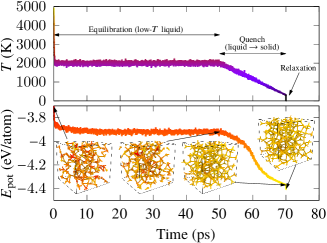
Figure 1: Melt-quench simulations of a-Si formation carried out with a GAP Bartók et al. (2010) potential refitted Caro (2021) from the database developed by Bartók et al. Bartók et al. (2018). The simulations were carried out with the TurboGAP code Caro et al. ; Caro (2019).

Additional steps can be added before or after the quench, typically some sort of annealing step. For instance, a carbon sample can be held at around 3500 K for a while before quenching to favor graphitization de Tomas et al. (2016, 2019); Wang et al. (2022). Or an a-Si sample can be annealed at a temperature below solidification (but still significantly higher than room temperature) to heal defects Deringer et al. (2018a).

The melt-quench process leading to generation of a computational atomic structure is exemplified for a-Si in Fig. 1. Initially, the sample, containing 216 atoms, has been heated to a very high temperature of 5000 K to properly randomize the atomic positions. The temperature is rapidly brought down to 2000 K, slightly above the melting temperature of silicon, and kept there for some time (50 ps in our example). This is the equilibration stage, where we aim to homogeneously distribute the available kinetic energy among all the degrees of freedom and find local structures which are low in energy (for the given values of $T$ and $P$). After equilibration, we quench the system down to 300 K using a linear temperature profile. The evolution of the potential energy does not follow this linear trend. Instead, there is a slow initial decrease in potential energy because the temperature is too high to create stable motifs. This is followed by an accelerated decrease in energy where these stable atomic motifs, tetrahedra in a-Si, are created at a fast pace. The final stage of the quench corresponds to slow further decrease in potential energy, because of either of two reasons: 1) all the Si atoms are already part of local tetrahedra or 2) there is not enough kinetic energy to overcome local potential energy barriers and the atoms are trapped into their local metastable structures. The actual situation is a combination of both factors. Recall that, according to the virial theorem, as we linearly decrease the kinetic energy there should be a corresponding linear decrease in potential energy, assuming that the details of the potential energy surface do not change. Therefore, the non-linear profile observed in our example is indeed associated to the phase transition from the disordered liquid to the amorphous solid.

After the MD quench, we further relax the structure using a static relaxation of the atomic positions, following a gradient-descent minimization of the potential energy. In Fig. 1 we have additionally color-coded the Si atoms according to their local energy, which can be extracted from a simulation with MLPs, as we detail in Sec. III. The curious reader is encouraged to visit the turbogap.fi website for a series of tutorials on how to run this type of simulation for a-Si and a-C.

Melt-quench simulations are popular because they provide a good compromise between CPU cost and the quality of the generated structures. However, they do not (typically) reproduce the experimental growth/formation protocol of the real material, and that can have a non-negligible effect on the resulting atomic structure, as is for instance the case for a-C Laurila et al. (2017). Unfortunately, direct simulation protocols, such as deposition in a-C Marks (2005); Caro et al. (2018a, 2020), are orders of magnitude more expensive than indirect methods.

Traditionally, direct simulation has been limited to empirical interatomic potentials Biswas et al. (1988); Luedtke and Landman (1989); Ramalingam et al. (2001); Marks (2005). These are very efficient computationally, relying on simple mathematical functions that depend on the interatomic distances and angles and are parametrized by fitting to experimental or first-principles data. Popular examples of these potentials, which can often be used for both Si and C (and even SiC) by adjusting the model’s parametrization, are Tersoff Tersoff (1988), Stillinger-Weber Stillinger and Weber (1985); Vink et al. (2001a), EDIP Bazant et al. (1997) (and its carbon version C-EDIP Marks (2000)), REBO Brenner (1990); Brenner et al. (2002) and ReaxFF Senftle et al. (2016); Van Duin et al. (2003); Srinivasan et al. (2015); Smith et al. (2017). However, these empirical potentials lack the accuracy of DFT, and thus provide a representation of the potential energy surface (PES) of very inconsistent quality Behler and Parrinello (2007); de Tomas et al. (2016); Bartók et al. (2018); de Tomas et al. (2019); Caro et al. (2020). While low-lying harmonic regions of the PES, i.e., the atomic configurations about equilibrium, can be reproduced with reasonable accuracy, chemical reactions are described very poorly. Therefore, we find ourselves at an impasse: on the one hand, the breaking and formation of chemical bonds, critical to understand the growth of amorphous materials, are not correctly described with affordable empirical potentials. On the other hand, DFT can describe chemical reactions accurately but is computationally unaffordable.

Fortunately, new atomistic simulation techniques based on machine learning (ML) have emerged in recent years Behler and Parrinello (2007); Bartók et al. (2010); Schütt et al. (2020) that bridge this huge gap in atomistic modeling of amorphous materials Deringer and Csányi (2017); Bartók et al. (2018). These MLPs rely on non-parametric fits to a reference PES, typically computed at the DFT level of theory Behler (2017); Deringer et al. (2021a). While still significantly more expensive than empirical force fields, MLPs offer accuracy close to that of DFT for a tiny fraction of the CPU cost. MLPs have had, in just the last few years, a huge impact on atomistic modeling of amorphous and disordered materials, granting us atomistic insight into problems that were completely out of reach less than a decade ago.

III ML interatomic potentials

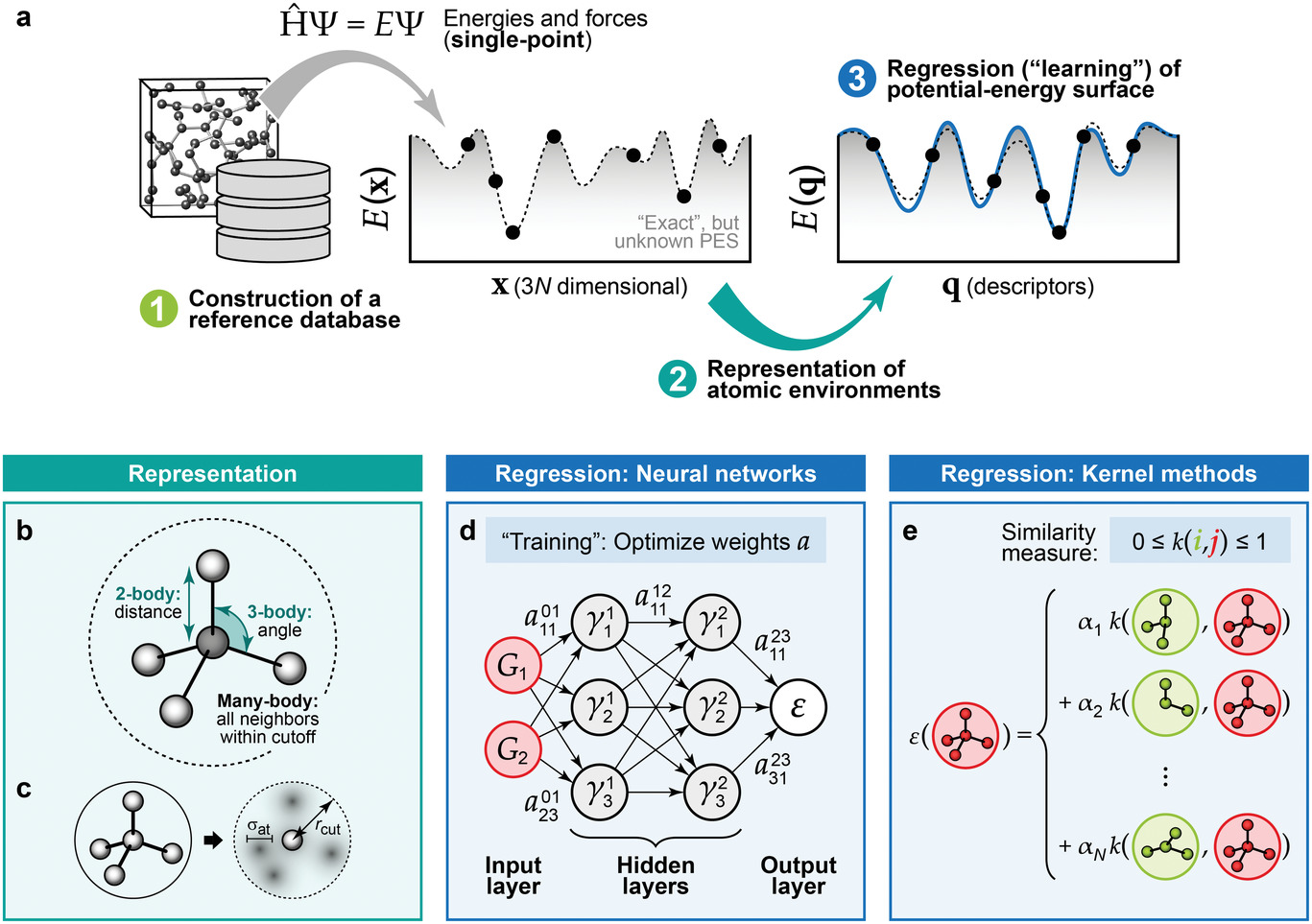
Figure 2: a) Workflow of MLP training: a database of atomic structures and observables (energies, forces) is constructed, from which an ML algorithm is used to learn the PES as a function of atomic descriptors. b,c) Different kinds of descriptors commonly used to represent the atomic environments. d) Schematics of neural network prediction. e) Schematics of kernel-based prediction. Reprinted from Ref. Deringer et al. (2019) with permission. Copyright (c) 2019 Wiley.

In this section we explain the whole MLP workflow, graphically summarized in Fig. 2. We start with a brief general introduction to different popular ways to represent the PES, with an emphasis on DFT. We will then give an overview of the two main methodologies for learning and interpolating the DFT-PES based on a) artificial neural networks (ANNs) and b) the related kernel-ridge regression (KRR) and Gaussian process regression (GPR) methods. To take a pedagogical approach, the introduction of these methodologies will be preceded by a general introduction to relevant ML concepts (databases and descriptors/features). We will compare ML potentials to DFT, on the one hand, and classical force fields, on the other, to get an idea of what is possible now in materials modeling, thanks to the introduction of MLPs, that was not possible just a few years ago. For more comprehensive information, the reader is referred to a recent book which nicely summarizes the current state of the field Schütt et al. (2020) including a chapter on GPR Csányi et al. (2020) and another on ANNs Hellström and Behler (2020), and to several overview papers Behler (2017); Bartók and Csányi (2015); Von Lilienfeld (2018); Shapeev (2016); Deringer et al. (2019, 2021a).

III.1 Database construction (structure selection)

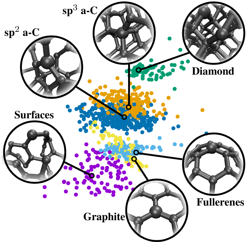
Figure 3: Low-dimensional embedding of high-dimensional data, used in this case to visualize the atomic structural diversity in a database constructed to fit an MLP for carbon. The closer two points are on the graph, the more closely the corresponding atomic environments resemble each other. Reprinted from Ref. Muhli et al. (2021) with permission. Copyright (c) 2021 American Physical Society.

The creation of a new MLP starts with the generation of training data (Fig. 2a, step 1). Many considerations need to go into carefully crafting a suitable database for the problem at hand. There are two main classes of MLPs depending on their scope: general- and single-purpose MLPs. A single-purpose MLP is created with a very specific application in mind. In this case, the MLP will be expected to perform with excellent (or even exquisite) accuracy for the problem of interest, but there is no guarantee that it will perform even reasonably for any other application. Recall that the MLP does not “know” about physics, chemistry, or the Schrödinger equation; it only knows about data. Therefore, an MLP will only be able to chart the portion of configuration space corresponding to the data that it was fed. Indeed, single-purpose MLPs (and poorly designed general-purpose MLPs) will tend to “blow up” (MD jargon for when a force field becomes catastrophically unstable) when tested on a problem for which they were not trained. A good example of a single-purpose MLP would be one trained to reproduce the phonon dispersion curves of a crystalline material, for instance to be used in thermal transport or thermal expansion calculations of c-Si and diamond/graphite. A database suitable to fit a good phonon MLP would typically incorporate many DFT calculations of structures distorted from the equilibrium ones, by adding either homogeneously spaced or random strain transformations to the unit cell in addition to rattling the atoms about their equilibrium positions. Furthermore, the unit cells should span from the primitive unit cell up to larger unit cells which would allow to capture interactions between distant atoms. An example of a single-purpose MLP is the graphene GAP of Rowe et al. Rowe et al. (2018).

A general purpose MLP, on the other hand, is expected to perform reasonably accurately in as many regions of configuration space as possible, and be resistant to blowing up. A good general-purpose MLP is often very difficult to achieve because it may require prior knowledge about which these regions are, and its training is consequently difficult to automate. For instance, if one wants to fit an MLP to study the atomic structure of a-C surfaces, which can be prohibitively expensive to generate with DFT using a melt-quench simulation (cf. Fig. 1), how are sample surfaces sourced for the (single-point) DFT calculations that will serve as reference for the MLP? In these cases, iterative training Deringer and Csányi (2017); Bernstein et al. (2019) can help in improving the accuracy of the MLP in regions of interest in configuration space and also to get rid of pathological behavior. In our a-C surface example, iterative training would consist of generating surface structures with an interim (low-quality) version of the MLP via melt-quench simulations. Single-point DFT calculations are then performed on the final structures and this data added to the training set. A new interim version of the MLP is trained and the whole procedure is repeated until the MLP errors (compared to the DFT calculations) are below an acceptable threshold. Besides regular sampling of known crystal phases, iterative training can also be combined with less directed exploration of configuration space, such as random structure search (RSS) Pickard and Needs (2011); Pickard (2022).

Finally, we can combine the features of a general-purpose MLP with those of a single-purpose MLP, to improve the accuracy of the general-purpose MLP for specific applications, as has been done for phonons in Si George et al. (2020) or fullerenes in C Muhli et al. (2021).

A way to visualize these structural databases is via so-called structure maps De et al. (2016); Cheng et al. (2020). In these, the similarities between different entries in a database, i.e., between different atomic structures, can be plotted on a two-dimensional map using low-dimensional embedding techniques De et al. (2016); Cheng et al. (2020). An example for the fullerene-augmented C MLP mentioned earlier Muhli et al. (2021) is shown in Fig. 3. In this graph, each data point represents an atom-centered environment and similar structures are clustered together. There is a transition from diamond structures to amorphous $sp^{3}$, then to amorphous $sp^{2}$ and finally to different graphitic structures, including fullerenes. These sketchmaps are a useful tool to glimpse at the composition of an entire database and understand the relationships between the different structures.

III.2 Reference representations of the potential energy surface

A central objective of computational atomistic modeling is to gain access to an accurate representation of the Born-Oppenheimer (BO) PES of a given ensemble of interacting atoms. The BO approximation relies on decoupling the electronic and nuclear degrees of freedom. That is, the BO-PES gives the total cohesive energy of a set of interacting atoms as the electronic ground state (GS) for fixed nuclear positions Martin (2004). This approximation is valid in many situations, in particular in condensed-matter physics, because of the mass difference between electrons and nuclei. The electronic degrees of freedom evolve within much shorter time scales than the nuclear degrees of freedom, and the atomic trajectories can be propagated in time treating the nuclei as classical particles, following Newton’s second law. The most popular approximation used today to calculate the BO-PES is DFT Hohenberg and Kohn (1964); Kohn and Sham (1965); Martin (2004). The fundamental tenet of DFT is that the total (cohesive) energy of a system of interacting electrons in a external potential (given by the positively charged nuclei) is given by a universal functional $E[n]$ of the electron density $n(\textbf{r})$, where the density that minimizes the functional is the GS density and the energy of the GS is given by the energy functional evaluated at the GS density Hohenberg and Kohn (1964):

$$n_{\text{GS}}(\textbf{r})=\underset{n(\textbf{r})}{\text{argmin}}\,E[n(\textbf{r})],\qquad E_{\text{GS}}=E[n_{\text{GS}}(\textbf{r})].$$ (1)

The practical means for solving Eq. (1) are provided by the Kohn-Sham (KS) ansatz, which states that the density can be expressed as a combination of single-particle contributions, one per electron (or electron pair, depending on whether or not spin is explicitly modeled):

$$n(\textbf{r})=\sum_{i=1}^{N_{\text{e}}}|\psi_{i}(\textbf{r})|^{2},$$ (2)

where $\psi_{i}(\textbf{r})$ is the KS orbital of the $i$th electron in the system and $N_{\text{e}}$ is the number of electrons. This approximation allows us to avoid explicitly working with the many-body wave function of the system. In the KS formulation of DFT, the many-body effects are collected into the exchange-correlation (XC) density functional $E_{\text{xc}}[n(\textbf{r})]$. The quality of the used approximation for $E_{\text{xc}}[n(\textbf{r})]$ will determine how close to the actual GS density and energy we can get.

The KS single-particle ansatz, coupled with the variational principle $\delta E[n]/\delta\psi_{i}^{*}=0$ leads to the eigenvalue-like KS equation:

$$\epsilon_{i}\psi_{i}(\textbf{r})=H_{\text{KS}}\psi_{i}(\textbf{r}),$$ (3)

where the KS Hamiltonian $H_{\text{KS}}$ contains the single-particle kinetic energy operator, the electrostatic potential and the XC potential. A deeper account of DFT is beyond the scope of this review, and the reader is referred to the excellent (nowadays almost standard) book by Martin Martin (2004) for more detailed information.

The emergence of KS DFT, together with many different approximations to the XC functional Perdew and Zunger (1981); Perdew et al. (1996) and efficient iterative algorithms for solving the KS equation implemented in parallel computer codes Kresse and Furthmüller (1996) have enabled quantum mechanical calculations of the properties of matter at affordable computational cost. In addition to this, the community has been very active at tackling the different shortcomings of KS DFT, such as the self-interaction error or the lack of dispersion interactions, e.g., by developing “hybrid” XC functionals Seidl et al. (1996); Heyd et al. (2003) and van der Waals “corrections” Grimme (2006); Tkatchenko and Scheffler (2009); Tkatchenko et al. (2012), respectively. While DFT is still too expensive to perform long- and large-scale simulations of atomic systems, the tradeoff between accuracy and CPU cost afforded by DFT makes it the most popular electronic structure method and, indeed, the most popular method to generate training data for MLPs.

The purpose of an interatomic potential, also referred to as a force field, is to provide a computationally affordable approximation of the BO-PES. When training MLPs we often assume that DFT provides a “good enough” version of the BO-PES. While we have just discussed that DFT has its own shortcomings, it is also important to recognize the limitations of the BO approximation itself. Notable breakdowns of the BO approximation occur whenever protium atoms are present (i.e., the common hydrogen isotope with one proton in the nucleus) Habershon et al. (2013) or when high-energy collisions take place (e.g., during radiation-damage events in materials) Darkins and Duffy (2018). Extended MD formalisms are required when simulating these kinds of systems, for instance time-dependent DFT (TD-DFT) or Ehrenfest dynamics, where electronic and nuclear degrees of freedom are propagated simultaneously Casida and Wesołowski (2004); Li et al. (2005). In addition, electronic excitations and charge-transfer processes Vlček Jr and Záliš (2007) cannot be captured out of the box by MLPs trained from DFT data. Despite these limitations, which are at the hot spot of current work by the community, MLPs have enabled incredible successes in computational materials modeling in recent years, in particular for a-Si and a-C. We review the basics of MLPs for materials and molecular modeling in the next section.

III.3 MLP architecture

The rationale for replacing a DFT calculation (or, more generally, an expensive ab initio calculation) by an ML prediction is that, in atomistic systems, the local atomic motifs are often repetitious. Therefore, put in simple terms, if we compute energies and forces for a series of reference structures with DFT and store those values in a database, we should in principle be able to infer a DFT-quality prediction for a new atomic structure as long as said structure is similar enough to the database entries. The interpolation should be computationally inexpensive, compared to a DFT calculation, for the procedure to be useful. The simplest example is a diatomic molecule, where a series of DFT calculations are carried out for different interatomic separations and a force field is trained from that data to predict the energy vs distance curve at arbitrary separations. An “old-fashioned” empirical force field would often tackle this problem by fitting the data to a fixed functional form, e.g., a least-squares fit to a second-order polynomial. In that sense, MLPs can be regarded as a glorified version of an empirical force field, where the main difference is the fact that the fit is now carried out in arbitrarily many dimensions and without the user providing an explicit mathematical function. This is referred to in ML jargon as a non-parametric fit. Although the distinction between MLPs and empirical force fields may seem small in this context, in practice the flexibility of ML algorithms to fit high-dimensional data means that much more complex PESs can be learned, and to much higher accuracy.

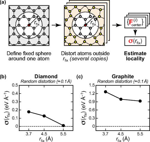
Figure 4: Locality tests in carbon-based systems. (a) Conceptualization of the locality test. (b) Convergence of the residual force acting on the central atom for diamond and graphite as a function of the cutoff radius. Reprinted from Ref. Deringer and Csányi (2017) with permission. Copyright (c) 2017 American Physical Society.

Above, two fundamental assumptions are made whose goodness will to a large extent determine the success of MLPs. One is the assumption of locality of the PES. That is, we can construct the entire system as a collection of local fragments, each of which has an associated local energy. Physically, the local energy $\bar{\epsilon}_{i}$ (where the bar indicates prediction) is not a well-defined property of the system; instead, a DFT calculation will return a total energy $E$ for a given ensemble of $N_{\text{at}}$ interacting atoms. An MLP will build this total energy from the sum of all the individual contributions which, in simplified terms, can be considered a sum over atom-wise contributions:

$$\bar{E}=\sum\limits_{i=1}^{N_{\text{at}}}\bar{\epsilon}_{i}.$$ (4)

An intuitive way to test the locality of the PES for a given material is to monitor the evolution of the force acting on an atom as other atoms beyond a certain cutoff distance are disturbed, as a function of said cutoff. This was done in Ref. Deringer and Csányi (2017) for crystalline and amorphous C. The procedure is illustrated in Fig. 4a and the results for diamond and graphite in Fig. 4b are reprinted from that reference. For diamond (as well as high-density a-C, not shown here but reported in Ref. Deringer and Csányi (2017)) the approximation of locality is extremely good and the errors are negligible for cutoffs around 5 Å and beyond. For graphite (and low-density a-C) the approximation is less good and convergence with the cutoff is very slow. Mathematically, this approximation implies that we can express a local (atomic) energy prediction as a function of a finite environment of the atom:

$$\bar{\epsilon}_{i}=f\left(S_{i}(r_{\text{cut}})\right),$$ (5)

where $S_{i}(r_{\text{cut}})$ represents all the relative atomic positions within a sphere of radius $r_{\text{cut}}$ centered on atom $i$. In technical terms this means that $\bar{\epsilon}_{i}$ has compact support.

The other main assumption is about the smoothness of the PES. That is, a small change in the positions of the nuclei should lead to a small change in the total energy of the system. In mathematical terms, the PES should be continuous and continuously differentiable. In a data science context, smoothness is referred to as regularity.

Besides the training (DFT) data and the two central approximations for the PES, locality and smoothness, which we have already discussed, an MLP requires also two basic ingredients. The first one is the atomic structure representation, which is carried out using atomic descriptors. While in principle the Cartesian coordinates of the nuclei contain all the necessary information, in practice they are not useful because they do not fulfill the correct symmetries. Specifically, valid atomic descriptors must fulfill translational, rotational and permutational invariance. The simplest descriptor is an interatomic distance. More sophisticated descriptors, which contain increasingly more information about the environment of an atom, can be constructed with a body-order expansion Allen et al. (2021). An interatomic distance is a two-body (2b) descriptor, with a single degree of freedom. A 3b descriptor has three degrees of freedom and perfectly characterizes a system made of three atoms, having subtracted the translation and rotation of the center of mass, which do not affect energy and forces. Any further body-order increase adds three more degrees of freedom, and the complexity of the model (and the cost of computing descriptors) explodes with relatively low body orders. For many practical purposes in materials modeling there is no need to go beyond 3b terms Christensen et al. (2020). However, there is another type of atomic descriptors that allow to encode the entire atomic environment, called many-body (mb) descriptors [cf. Fig. 2c]. Arguably, the most important examples are the smooth overlap of atomic positions (SOAP) Bartók et al. (2013) and atom-centered symmetry functions (ACSFs) Behler (2011). It can be shown that these mb descriptors are formally equivalent to one another and, as constructed from 2b sums within a finite cutoff sphere, are also equivalent to an ensemble of 3b terms Willatt et al. (2019). Two advantages over 3b descriptors are that one mb descriptor can be used instead of very many 3b ones (since the number of 3b descriptors within a cutoff sphere explodes as a function of its radius), and that mb descriptors with different numbers of atoms can be compared to one another (directly relevant in kernel regression methods, cf. Fig. 2e). The topic of atomic representations is very rich and has been recently summarized in a comprehensive review paper Musil et al. (2021).

The second basic ingredient is the machine learning algorithm. The first method to interpolate high-dimensional PES with close to DFT accuracy was introduced in 2007 by Behler and Parrinello Behler and Parrinello (2007) based on ANNs and applied precisely to model Si. The second method, based on kernel regression, was introduced by Bartók et al. in 2010 Bartók et al. (2010) and used to model C, Si and Ge. Clearly, group-IV semiconductors have been strongly linked to the use of MLPs since their very inception, and as such it is unsurprising that the first applications of MLPs to solving outstanding problems in materials modeling have also focused on C and Si. Naturally, the methodology has advanced significantly since those two seminal papers and more recent reviews by the authors do a better job at introducing the concepts and practicalities to the beginner Bartók and Csányi (2015); Behler (2017); Deringer et al. (2021a). Many other methods and implementations have appeared since then. A comprehensive account of those is beyond the scope of this work and so we mention again the recent book summarizing the state of the field Schütt et al. (2020). Below we give a brief overview of these methods, and refer the reader to the cited literature for further detail.

Artificial neural network potential (NNP). NNPs Behler and Parrinello (2007) use artificial neural networks (ANNs) to interpolate the PES. An ANN consists of a series of “layers”: input, hidden and output layers. There is one input and one output layer, and one or more hidden layers. The input layer contains a vector of features (an ACSF in the case of NNPs) and the output layer returns an observable, which can be a scalar or a vector (e.g., the total energy in NNPs). Each hidden layer consists of a number of nodes, and the input data is propagated forward through the different layers by performing a series of linear and non-linear operations which depend on the connection and the node in question, respectively. This propagation procedure is illustrated in Fig. 2d, where the arrows represent the connections and the circles represent the nodes. We start out with a vector of real-valued symmetry functions G of a certain dimension, which depends on the number of species and the quality of the representation Behler (2011); Hellström and Behler (2020). Each of these functions $G_{i}$ is propagated to each of the nodes in the first hidden layer multiplied by a series of weights $a^{0,1}_{ij}$ (where 0,1 indicates we are connecting layers 0 and 1):

$$\beta^{1}_{j}=\sum\limits_{i=1}^{N_{0}}G_{i}a^{0,1}_{ij}+b^{1}_{j},$$ (6)

$$\gamma^{1}_{j}=f(\beta^{1}_{j}),$$ (7)

where $N_{0}$ is the number of nodes in layer 0, i.e., the number of ACSFs (or, equivalently, the dimension of G) in this case. $b^{1}_{j}$ is the bias of node $j$ in layer 1 which, together with the sum in Eq. (6), define the function $\beta^{1}_{j}$, which is linear in the input variable $G_{i}$. This quantity, $\beta^{1}_{j}$, is used as argument to evaluate a non-linear activation function $f$. The result of this evaluation, $\gamma^{1}_{j}$, is then passed on to the next layer $n=2$ in the same way as above:

$$\beta^{n}_{j}=\sum\limits_{i=1}^{N_{n-1}}\gamma_{i}^{n-1}a^{n-1,n}_{ij}+b^{n}_{j},$$ (8)

$$\gamma^{n}_{j}=f(\beta^{n}_{j}),$$ (9)

where we note that $N$ can in general vary from layer to layer. We have substituted $G_{i}$ by $\gamma_{i}^{n-1}$ for generality, because $G_{i}$ is the notation used for the input layer specifically in the case of ACSF for NNPs. This procedure is repeated until we reach the output layer, which in our case returns a local atomic energy. The forces can be evaluated analytically from the dependence of the symmetry functions on the atomic positions.

Training an NNP consists in the optimization of the weights $\{a^{n-1,n}_{ij}\}$ and biases $\{b^{n}_{j}\}$, and is done using backpropagation, for a given training set of atomic structures, to minimize the error in the corresponding observables (total energies, forces, stresses, etc.). We will not go into the details of ANN algorithms which, for most practical purposes in atomistic materials modeling, can be considered a black box.

Gaussian approximation potential (GAP). GAPs are based on kernel regression Bartók et al. (2010) and are arguably more interpretable than ANNs. In GAPs, the local atomic energy $\bar{\epsilon}_{i}$ for atom $i$ is expressed as a linear combination of kernel functions $k$:

$$\bar{\epsilon_{i}}=\delta^{2}\sum\limits_{t=1}^{N_{\text{train}}}\alpha_{t}k(\textbf{q}_{i},\textbf{q}_{t})+e_{0},$$ (10)

where $\delta$ is an energy scale, $t$ runs over training configurations, $\alpha_{t}$ are the fitting coefficients, $\textbf{q}_{i}$ and $\textbf{q}_{t}$ are the atomic descriptors (often a SOAP mb descriptor) of a test and train configuration, respectively, and $e_{0}$ is a per-atom energy offset, usually taken as the reference energy of an isolated atom of a given species. The kernel can be understood as a measure of similarity between two atomic environments, as illustrated in Fig. 2e, and is bounded between 0 (nothing alike) and 1 (identical up to symmetry operations). Thus, intuitively, the more a training configuration resembles the test configuration for which we want to make a prediction, the more the fitting coefficient associated with that training configuration contributes to the prediction. This is why we stated earlier that GAPs are arguably more interpretable than NNPs.

Having cast the interpolation problem as a linear problem, training a GAP simply consists in a least-squares-based inversion of Eq. (10):

$$\bm{\alpha}=\frac{1}{\delta^{2}}\textbf{K}^{-1}(\bm{\epsilon}-\textbf{e}_{0}),$$ (11)

where now the test index in Eq. (10) also runs through training configurations, and we do not use the predicted atomic energy $\bar{\epsilon}$ but the observed one $\epsilon$. We note that in practice one cannot train a GAP model (or an NNP, for that matter) using local atomic energies, which are not generally available before training the GAP. Instead, the local energy in Eq. (10) is replaced by the sum over local energies leading to a total energy observable. For instance, when using training data from a DFT calculation for a supercell, we use $E_{I}=\sum_{i}\bar{\epsilon}_{i}$. In addition to this total energy consideration, one usually needs to use regularization and sparsification to improve the stability, transferability and efficiency of a GAP, and may combine several GAPs in the same fit. These details fall outside the scope of this paper and the reader is referred to the literature for further insight Bartók and Csányi (2015); Deringer et al. (2021a). Likewise, the explicit definition and discussion of atomic descriptors and kernel functions is an active research topic and better covered elsewhere Bartók et al. (2013); Caro (2019); Willatt et al. (2019); Himanen et al. (2020); Musil et al. (2021). As for NNPs, the forces can be computed analytically through the dependence of $\textbf{q}_{i}$ on the atomic positions. Forces and stresses can also be incorporated into the inversion equation, together with total energies.

Other MLP approaches. The field of ML-based atomistic simulation of materials is advancing fast. Since NNPs and GAPs appeared, several other MLP flavors have been developed and we expect applications in amorphous materials modeling to follow soon. MLP methods besides NNP and GAP include “linear” models such as the moment-tensor potential (MTP) Shapeev (2016) and the spectral neighbor analysis potential (SNAP) Thompson et al. (2015), or MLPs based on asymptotically complete atomic descriptors like the atomic cluster expansion (ACE) Drautz (2019). The first ACE-based MLP able to simulate a-C appeared very recently Qamar et al. (2022), and it is expected that these new models and improvements thereof Batatia et al. (2022); Darby et al. (2022) will overtake NNPs and GAPs as the state-of-the-art tools for simulating disordered materials in the near future.

In the brief discussion of NNPs and GAPs above we implicitly include short-range interactions only, since ACSFs and SOAP use radial cutoffs that exclude all interactions beyond a certain radius. We have therefore left out long-range interactions which are important beyond the typical cutoffs used to fit “regular” MLPs. These long-range interactions include van der Waals and electrostatics and must be treated on a different footing to bonding and repulsion interactions both i) out of necessity, to avoid the explosion of computational time with the cutoff distance, and ii) out of opportunism, since these interactions can often be cast in the form of simple analytical functions whose parameters can be machine learned but are in effect short ranged Bereau et al. (2018); Veit et al. (2020); Xie et al. (2020); Muhli et al. (2021); Staacke et al. (2022).

IV Amorphous and disordered carbon

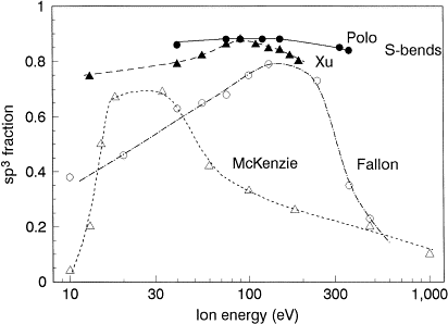
Figure 5: (Top) $sp^{3}$ fraction vs deposition energy from a series of literature works; data from Polo et al. Polo et al. (2000), Xu et al. Xu et al. (1997), Fallon et al. Fallon et al. (1993) and McKenzie et al. McKenzie et al. (1991). The deposition energy is the estimated kinetic energy of individual carbon atoms as they hit the substrate. (Bottom) The subplantation mechanism postulated as growth mechanism responsible for high $sp^{3}$ fractions in ta-C. Both figures reprinted from Robertson Robertson (2002) with permission. Copyright (c) 2002 Elsevier.

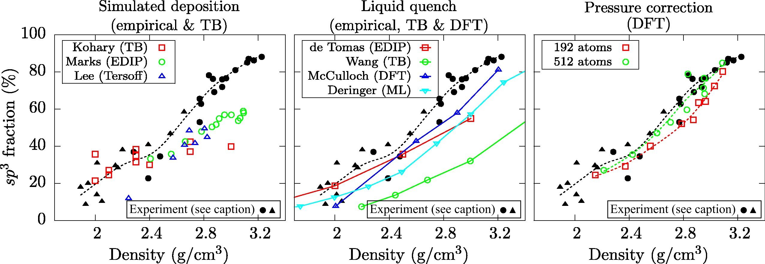
Figure 6: $sp^{3}$ fractions vs mass density for different simulation protocols, compared to experimental data (black solid dots) from Fallon et al. Fallon et al. (1993) and (black solid triangles) Schwan et al. Schwan et al. (1996). Simulation data from Kohary and Kugler Kohary and Kugler (2001), Marks Marks (2005), Lee et al. Lee et al. (2004), de Tomas et al. de Tomas et al. (2016), Wang and Komvopoulos Wang and Komvopoulos (2014), McCulloch et al. McCulloch et al. (2000) and Deringer and Csányi Deringer and Csányi (2017). Pressure-corrected DFT data is taken from Caro et al. Caro et al. (2014) for 192-atom supercells and Laurila et al. Laurila et al. (2017) for 512-atom supercells. Reprinted from Ref. Laurila et al. (2017).

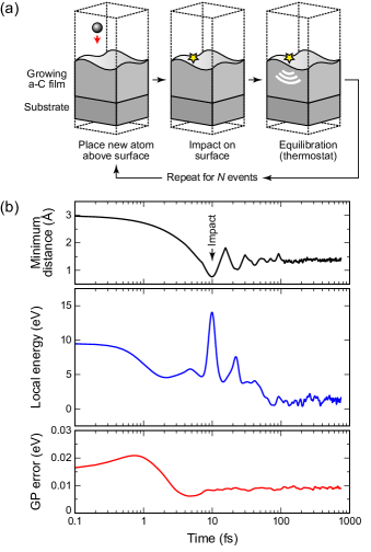
Figure 7: (a) Schematics of a deposition simulation. (b) Evolution of different observables during the course of a single impact event. Reprinted from Ref. Caro et al. (2020) with permission. Copyright (c) 2020 American Physical Society.

(a)

(b)

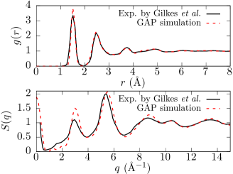
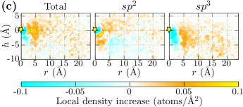
Figure 8: Results of ta-C deposition simulations: (a) Evolution of mass density and coordination fractions along the film’s growth direction in ta-C over three different deposition energies. The extent of the $sp^{2}$-rich surface, different for each energy, is indicated with an arrow; (b) Radial distribution function and structure factor, compared to experimental results from Gilkes et al. Gilkes et al. (1995); (c) Two-dimensional pair-correlation functions indicating the regions of depletion/formation of $sp^{2}$ and $sp^{3}$ motifs as a function of distance from impact location. Reprinted from Ref. Caro et al. (2018a) with permission. Copyright (c) 2018 American Physical Society.

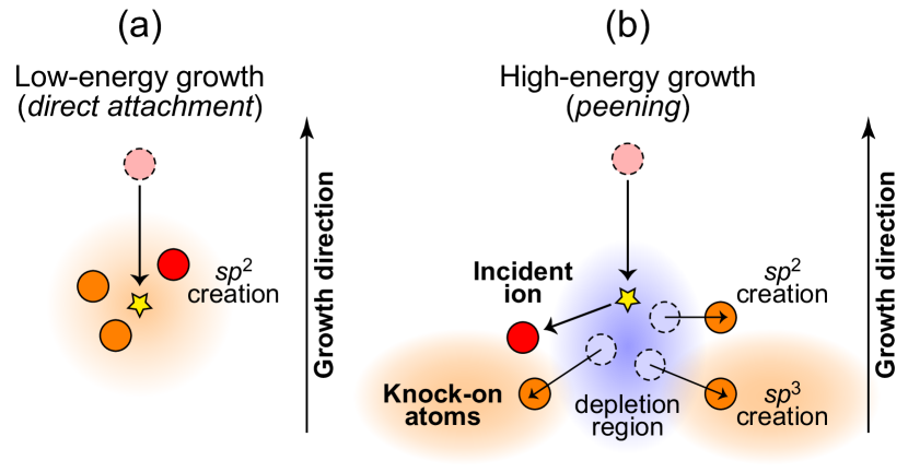
Figure 9: Observed growth mechanisms in (a) low-density (low deposition energy) and (b) high-density (high deposition energy) a-C films. Reprinted from Ref. Caro et al. (2020) with permission. Copyright (c) 2020 American Physical Society.

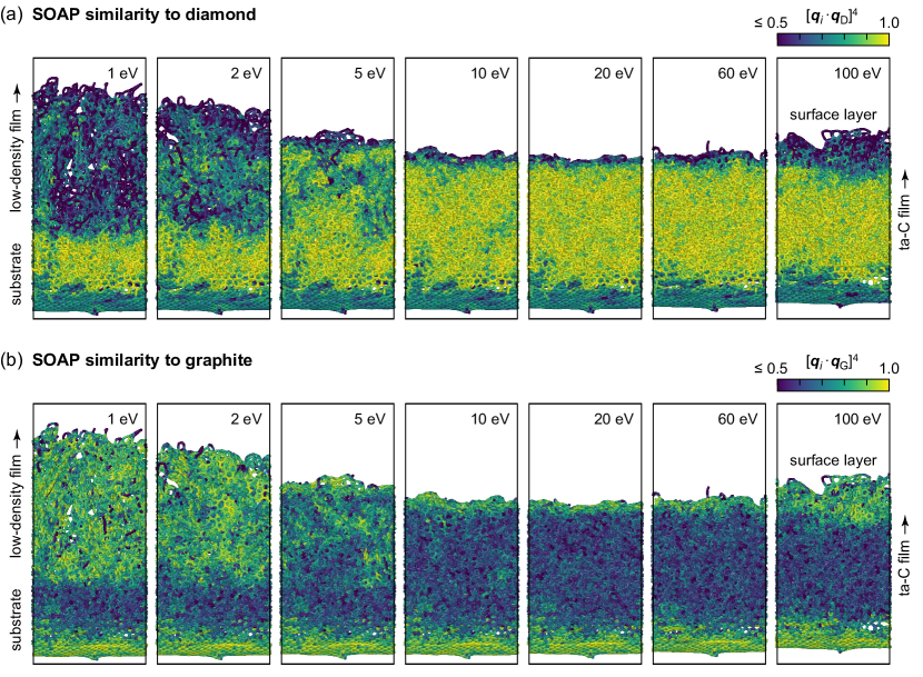
Figure 10: Evolution of a-C film nanostructure as a function of deposition energy. The top (a) and bottom (b) panels show the degree of similarity between atomic environments in the films and reference diamond and graphite, respectively. Brighter color indicates more resemblance and darker color indicates less resemblance. Reprinted from Ref. Caro et al. (2020) with permission. Copyright (c) 2020 American Physical Society.

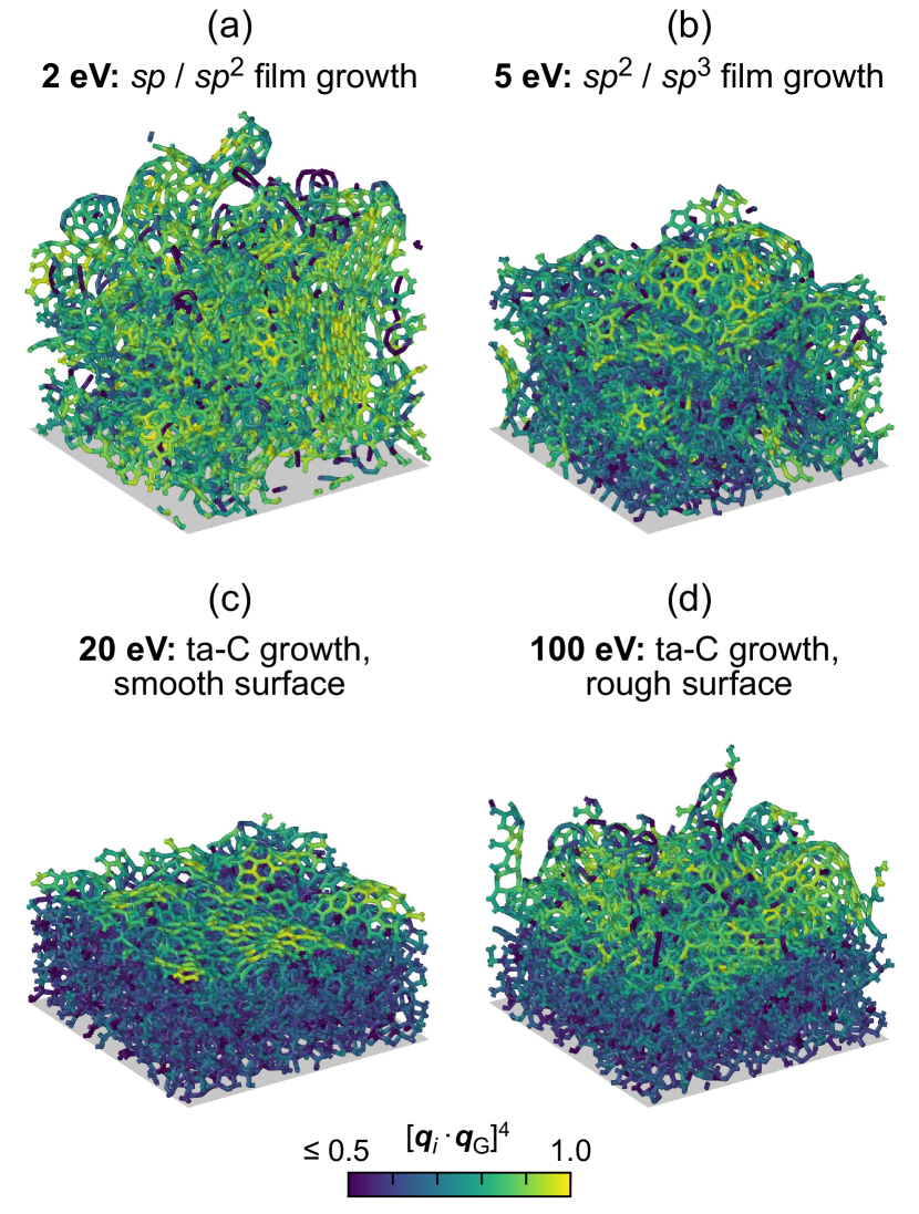
Figure 11: Detail of the surface nanostructure in a-C films grown at different deposition energies, indicating the atomic motifs similarity to graphite. Reprinted from Ref. Caro et al. (2020) with permission. Copyright (c) 2020 American Physical Society.

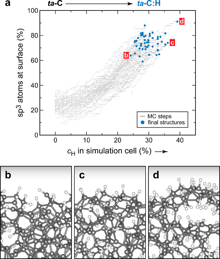
Figure 12: a) $sp^{3}$ fraction of hydrogenated a-C as a GCMC simulation progresses where H is incorporated. The blue dots mark the end points of the simulation. b-d) Ball-and-stick representation of the final a-C:H structures. Reprinted from Ref. Deringer et al. (2018b) with permission. Copyright (c) 2018 American Chemical Society.

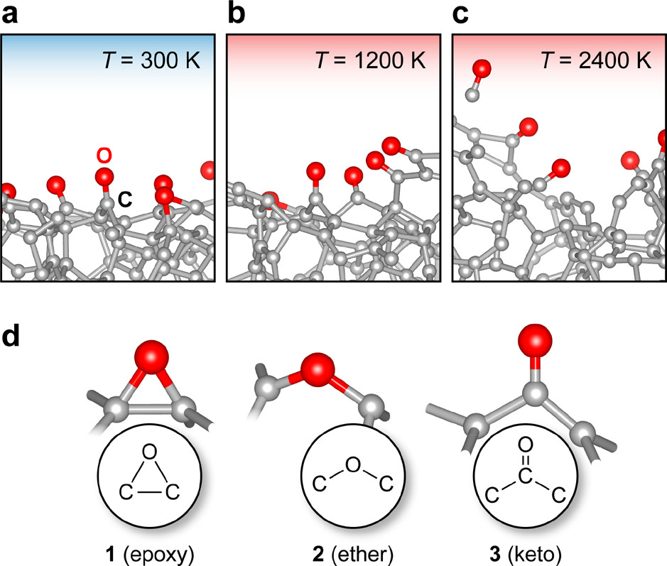
Figure 13: a-c) Ball-and-stick representation of a-C:O DFT-MD simulations carried out at different temperatures. d) Most representative O-containing motifs present in the resulting a-C:O structures. Reprinted from Ref. Deringer et al. (2018b) with permission. Copyright (c) 2018 American Chemical Society.

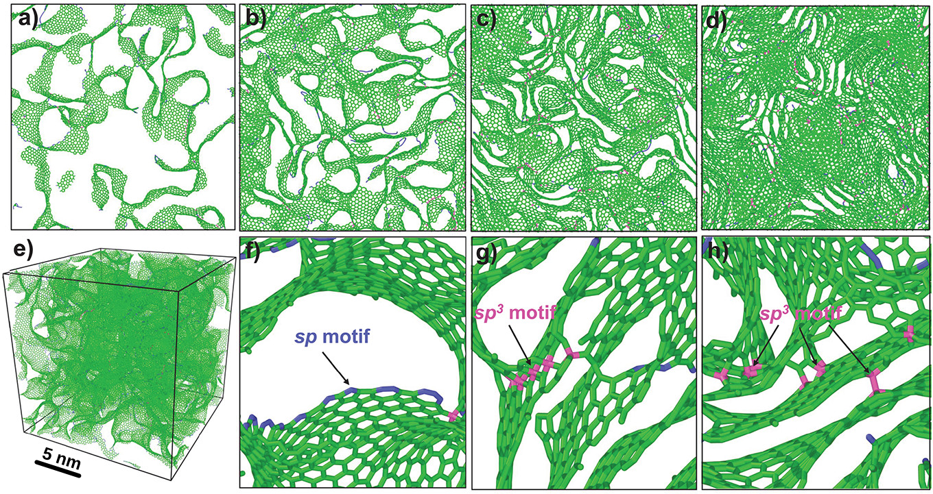
Figure 14: a-d) Nanoporous carbon structures of different densities, where the density increases to the right and the average pore size decreases correspondingly. e) 3D model of the low-density nanoporous carbon structure from a), where the pore morphology can be more easily appreciated. f-h) $sp$ motifs are found in graphitic sheet termination (edges) and $sp^{3}$ motifs are found interlinking stacked graphitic layers, conferring three-dimensional rigidity to these nanoporous carbon networks. Reprinted from Ref. Wang et al. (2022).

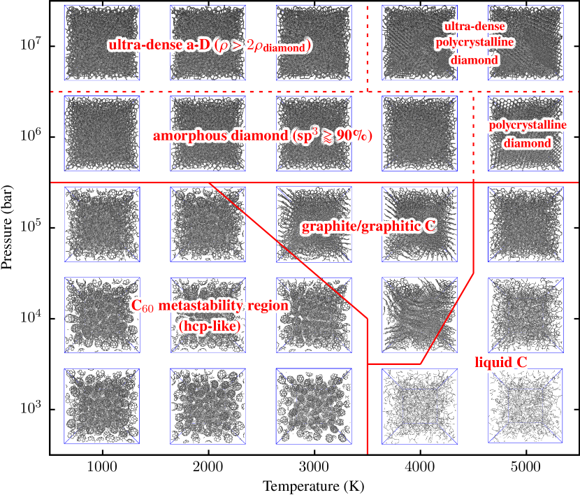
Figure 15: High-pressure/high-temperature phase diagram of C₆₀, where the molecular precursor leads to nucleation of high-density ta-C (“amorphous diamond”) as the molecular C₆₀ collapse at high pressure. Reprinted from Ref. Muhli et al. (2021) with permission. Copyright (c) 2021 American Physical Society.

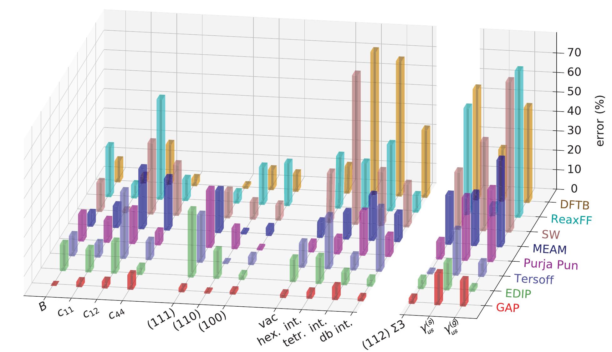
Figure 16: Comparison between the silicon GAP18 and other force fields for predicting a number of properties; from left to right: elastic moduli, surface energies, point defect formation energies, and planar defect formation energies. Reprinted from Ref. Bartók et al. (2018).

Deringer et al.

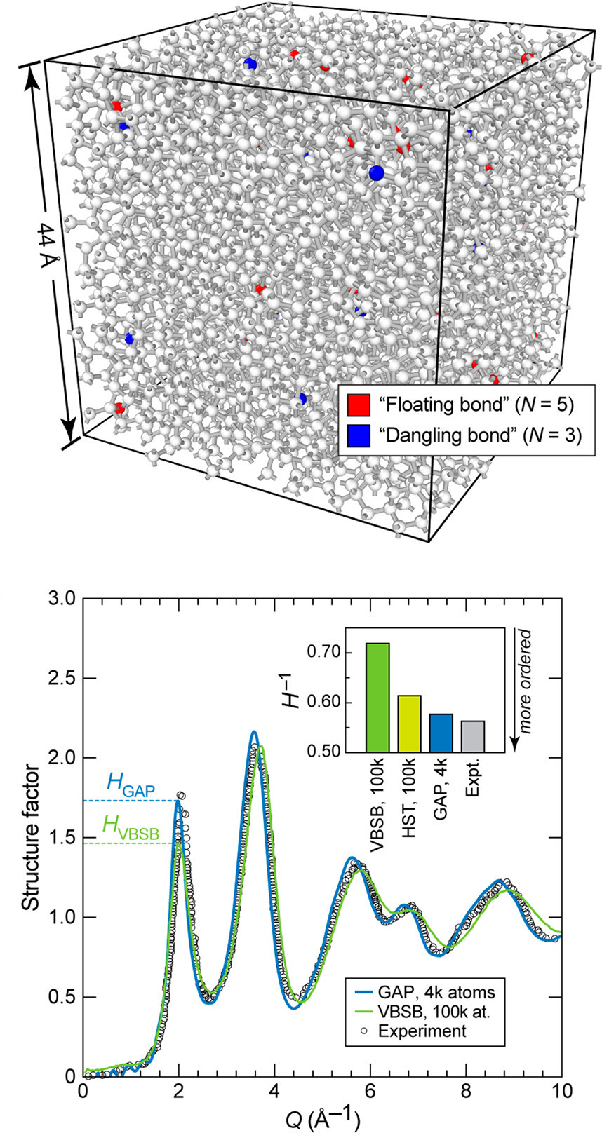
Wang et al.

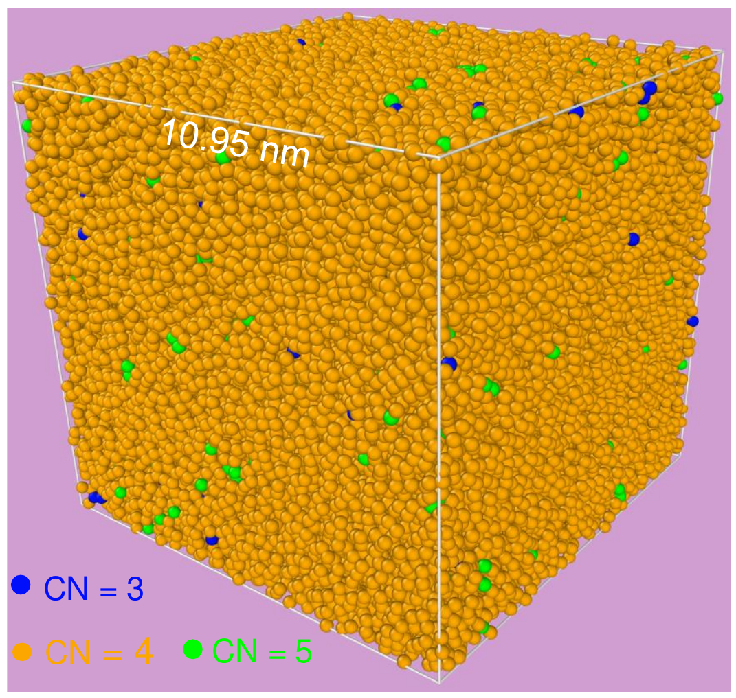
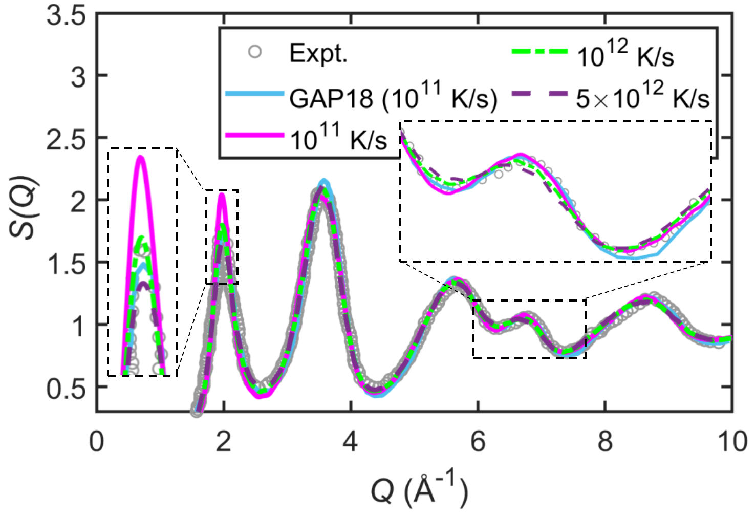
Figure 17: Computational a-Si structural models and their corresponding structure factor from Deringer et al. Deringer et al. (2018a) (left panels) and Wang et al. Wang et al. (2023) (right panels). Deringer’s structure factor is compared to that derived from preexisting structural models from the literature, VBSB Vink et al. (2001b) and HTS Hejna et al. (2013), and to experiment. Wang shows the effect of the annealing rate on the structure factor and a direct comparison to Deringer’s data (labeled GAP18). In both cases the experimental data is from Laaziri et al. Laaziri et al. (1999a, b). Deringer et al. figures reprinted from Ref. Deringer et al. (2018a). Wang et al. figures reprinted from Ref. Wang et al. (2023) with permission. Copyright (c) 2023 American Physical Society.

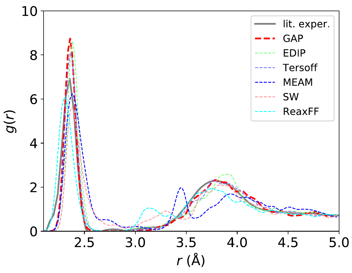
Figure 18: GAP results for the RDF of a-Si from Bartók et al. Bartók et al. (2018), and comparison to the RDF obtained from experiment Laaziri et al. (1999a, b) and using different popular interatomic force fields for silicon. Reprinted from Ref. Bartók et al. (2018).

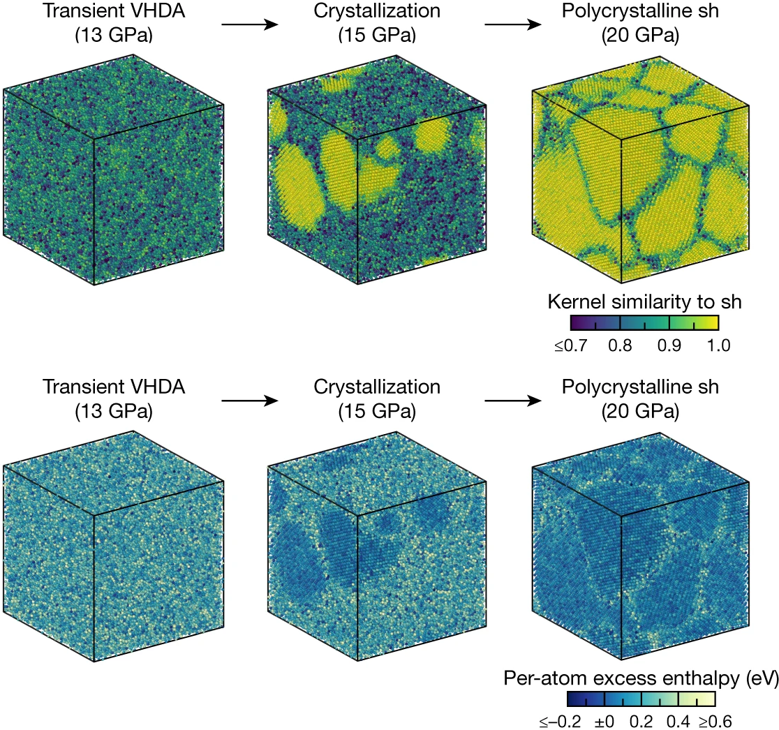
Figure 19: High-pressure phase transition in silicon from a very-high-density amorphous (VHDA) phase to a (metallic) polycrystalline phase. Reprinted from Ref. Deringer et al. (2021b) with permission. Copyright (c) 2021 Springer Nature.

The precise structure of a-C and how growth conditions can be tuned to modify it have been the topic of intense debate for several decades. The reason is that, unlike in a-Si, in a-C coordination environments with different number of atomic neighbors, ranging from two to four neighbors ($sp$ and $sp^{3}$ orbital hybridizations, respectively) are all possible (meta)stable motifs. Especially three- ($sp^{2}$) and four-coordinated environments can coexist in a-C thin films. Varying the relative concentration of $sp^{2}$ and $sp^{3}$ bonding in a-C allows us to tune its material properties (mechanical, electrical, optical, etc.) from graphite-like to diamond-like. Thus, much of the basic characterization work on a-C has dealt with the dependence of the $sp^{2}$/$sp^{3}$ ratio on such parameters as the deposition energy during physical vapor deposition (PVD) growth and, in turn, the dependence of the material properties on the $sp^{2}$/$sp^{3}$ ratio. The reference entry point into the properties of a-C, albeit a bit outdated in terms of missing atomistic simulation insights that were developed in the last few years, is Robertson’s monumental review paper from 2002 Robertson (2002). Two of the most important figures in that paper are reprinted here in Fig. 5. The top panel shows the dependence of the $sp^{2}$/$sp^{3}$ ratio on the deposition energy (the estimated kinetic energy of incident C atoms) for different experimental techniques used to grow a-C. A common trend is the increase in $sp^{3}$ content for increasing deposition energy, up to around 100 eV, after which there is a further decline. We also note that some of these a-C samples can be grown with extremely high $sp^{3}$ contents, approaching that of diamond (100 % $sp^{3}$). Therefore, diamondlike or “tetrahedral” a-C (DLC and ta-C, respectively) can be made experimentally, offering a route for cheap coatings with diamondlike hardness for tribological applications. The bottom panel in Fig. 5 shows the proposed film growth mechanism in ta-C, subplantation, which was widely regarded as the correct mechanism until recently, when MLP simulations Caro et al. (2018a) provided quantitative confirmation for earlier qualitative evidence Marks (2005) of an alternative mechanism, peening, which we will discuss later in more detail.

Thus, our journey into simulation of a-C starts with the extensive atomistic modeling efforts carried out in the pursuit of explaining how these high $sp^{3}$ contents can be achieved and, in turn, explaining the growth mechanism in a-C. The state of the art in atomistic modeling of a-C, as of 2017 (just 6 years before this review was completed), using a variety of interatomic potentials (including DFT) and modeling techniques, is summarized in Fig. 6. This figure was compiled right after the first MLP able to model a-C was published, also in 2017 Deringer and Csányi (2017). We can see that the direct simulation route, deposition, fell short of achieving the very large $sp^{3}$ contents observed experimentally at high deposition energies. This technique had, back in the day, been restricted to fast empirical methods, such as tight binding (TB), C-EDIP and Tersoff potentials, and was (and still is) computationally unfeasible at the DFT level. Liquid quench simulations, on the other hand, were accessible to more expensive methods, like DFT, but could only predict very large $sp^{3}$ contents at unphysically high pressures, which shows as a shift towards higher mass densities on the graph. On that middle panel of Fig. 6 we note the first ML-based simulations of a-C generation with the MLP trained by Deringer and Csányi Deringer and Csányi (2017), a stepping stone in a-C modeling and key development leading to the advances that we will discuss later. Finally, pressure-corrected DFT simulations from Refs. Caro et al. (2014); Laurila et al. (2017), based on a two-step relaxation procedure, managed to get extremely good agreement with experiment for the $sp^{3}$ content as a function of mass density but, based on an indirect simulation protocol, offered no insight whatsoever into the growth mechanism.

Explaining the growth mechanism. With the introduction in 2017 of the first MLP able to handle the structural complexity of a-C with close to DFT accuracy, but at a fraction of the computational cost, the first MLP-based simulation depositions followed soon. In 2018, Caro et al. Caro et al. (2018a) presented MD deposition simulations of ta-C growth. In these simulations, incident atoms with varying kinetic energy (20, 60 and 100 eV) impinge on a carbon substrate, initially diamond. After each impact, the system is equilibrated back to the nominal deposition temperature (300 K) and the next deposition event takes place. After several thousands of atoms have been deposited, the size of the film is enough to collect statistics for material properties and growth mechanism. The workflow of these deposition simulations is shown in Fig. 7(a). Panel (b) of the figure shows a more detailed view of the impact process for a single event with a logarithmic time axis. Initially, the incident atom approaches the substrate very fast. The MLP algorithm allows us to monitor the local atomic energy, as we have discussed in Sec. III.3, shown in the figure offset by the average local energy in the growing film. The highly energetic initial impact is followed by equilibration of the atomic environment, where atoms settle in their new positions. GAP MLPs also allow us to monitor the predicted interpolation error, shown in the figure too. This deposition process is rather complex, with the order of 50 bond breaking/formation events taking place for each impact at around 100 eV Caro et al. (2020). The process is better visualized as a video animation, with several Open Access resources available from the literature, including a single impact Caro (2020a), the atom-by-atom growth of a-C thin films from low to high density Caro (2017), and the resulting atomic structures in XYZ format Caro (2020b) (which enable subsequent studies).

Figure 8 shows the key results from these first deposition simulations Caro et al. (2018a). Panel (a) shows the mass density and $sp$/$sp^{2}$/$sp^{3}$ fraction profiles along the growth direction for the deposition energy ranges where ta-C growth takes place. The three simulations at 20, 60 and 100 eV result in similar mass densities and coordination fractions in the bulk of the film, for the first time close to those reported experimentally for the densest ta-C films. At the same time, the data shows rather different surface morphologies, with increasing surface roughness for higher deposition energies, a result that closely follows experiment Davis et al. (1998). This, together with the also excellent agreement with experiment for the radial distribution function (RDF) shown in Fig. 8(b) gave confidence in the quality of the simulations as representative of the microscopic growth mechanism taking place experimentally. The collection of deposition statistics (up to 8000 individual events per energy) then enabled drawing a precise picture of what that growth mechanism actually looks like. In Fig. 8(c) we can see the mass density and coordination fraction increase/decrease before and after an impact event, averaged over all impacts, as a function of depth and lateral separation from the impact site. The color maps clearly indicate a local decrease of $sp^{2}$ and, especially, $sp^{3}$ carbons around the site of impact. In fact, these maps show that locally (around the impact site) there is an increase in the amount of $sp^{2}$ carbon, whereas the $sp^{3}$ fraction increases laterally and away from the impact site, due to pressure waves originating from the impact region. This mechanism is known as peening, and had already been proposed by Marks in 2005 on the basis of deposition simulations with the C-EDIP empirical potential Marks (2005). Because the C-EDIP simulations lacked quantitative agreement with experiment [cf. Fig. 6], the peening mechanism did not gather generalized adoption. However, the GAP deposition simulations offer strong quantitative support for peening as the growth mechanism in ta-C, which is schematically illustrated in Fig. 9(b).

a-C structure across mass densities. Following the study of ta-C growth, these deposition simulations were extended to low-density a-C and a more comprehensive analysis of material properties and comparison with other interatomic potentials was carried out Caro et al. (2020). At low deposition energies (below the typical cohesive energy per atom in carbon materials, $\lessapprox 9$ eV), graphitic a-C grows by direct attachment [Fig. 9(a)], where higher coordination increases the stability of $sp$ surface motifs by creating $sp^{2}$ and $sp^{3}$ carbon. At very low deposition energies of a couple of eV the rate of $sp^{3}$ formation is small and the bulk of the a-C films is highly graphitic, with $\sim 80$ % $sp^{2}$ and similar amounts of $sp$ and $sp^{3}$ motifs ($\sim 10$ % each). Figure 10 shows the evolution of the structure, as well as the “graphite likeness” and “diamond likeness”, of the simulated thin films as a function of deposition energy. The similarity to graphite and diamond is computed by calculating the SOAP kernels between each individual atomic environment and either pristine graphite or diamond Deringer and Csányi (2017); Caro et al. (2020). Since the kernel can be understood as a similarity measure, bounded between 0 and 1, as we have previously discussed, it can also be used for this kind of quantitative comparison in a very straightforward way. At and above $\sim 10$ eV the structure is largely homogeneous and dominated by $sp^{3}$ motifs in the bulk of the film. At 5 eV $sp^{2}$ and $sp^{3}$ motifs are approximately equally frequent, and the material shows a “patched” structure. At low deposition energies the material is graphitic in nature, as we have already discussed, and made of tubular (nanotube-like) structures and highly defective graphitic sheets.

a-C surface structure. The surface structure in a-C is always graphitic like (Figs. 8 and 10), but the extent of this $sp^{2}$-rich surface layer is strongly dependent on the deposition energy. The MLP deposition simulations show a smoothest surface at around 20 eV and roughest at 100 eV (and, presumably, higher energies, which have not been studied) Caro et al. (2018a). For very low deposition energies there is no well-defined surface region, except for a higher relative abundance of $sp$ motifs within the top 10 Å or so, and the film is graphitic and highly disordered throughout. A closeup on the structure of a-C surfaces for different mass densities, again color coding according to graphite likeness, is given in Fig. 11.

Doped a-C. As-deposited a-C is rarely completely free of impurities. Residual elements present in the reactor chamber and sample setup lead to unintentional doping of a-C films with a wide range of chemical species, the most significant of which are H, O, N and Si (see, e.g., time-of-flight elastic recoil detection analysis [ToF-ERDA] Mizohata (2012) results of the elemental makeup of a-C:N Etula et al. (2021)). Besides unintentional doping, it is possible to incorporate impurities in order to achieve a desired effect. The mechanical, electronic and (electro)chemical properties of a-C can be modified via H, O and N incorporation Robertson (2002); Santini et al. (2015); Etula et al. (2021). Intentionally doped a-C is usually denoted by a-C:X, where X stands for the dopant. The most common doped form of a-C is hydrogenated a-C, or a-C:H, where typical H contents are of the order of 30–50 at.-% Robertson (2002). This material can be made for instance by depositing C in a H/methane plasma, or by depositing acetylene or methane molecules directly, depending on the desired C/H ratio Robertson (2002). The properties of a-C:H differ from those of a-C in that H atoms will saturate many bonds, potentially leading to high $sp^{3}$ contents but relatively low mass densities, because a H atom is about 12 times as light as a C atom. The mechanical properties of a-C:H, e.g., its elastic moduli, will be inferior to those of ta-C with similar $sp^{3}$ content Robertson (2002).

Computational studies on a-C:H are comparatively rare, and direct deposition simulations of a-C:H with MLPs are not yet available in the literature (although our group is currently exploring this possibility). Indirect simulations of a-C:H formation and H adsorption energetics mixing MLPs and DFT or other electronic-structure methods have appeared in recent years. Ref. Deringer et al. (2018b) did grand-canonical Monte Carlo (GCMC) simulations of H adsorption using density-functional tight binding from a wide set of preexisting a-C surface models. These results showed that a-C:H materials with very high $sp^{3}$ fractions ($\sim$ 75%) can be obtained over a relatively large range of H concentrations (ranging from 25% to 40%). The results of these GCMC trajectories and snapshots of the resulting films are given in Fig. 12. Ref. Caro et al. (2018b) focused on the individual adsorption processes and how those depend on the geometry of the preexisting pure carbon sites, finding two separate regions of adsorption stability for $sp$ and $sp^{2}$ sites each. Almost-linear and almost-planar $sp$ and $sp^{2}$ motifs, respectively, are more stable and therefore less reactive towards H adsorption than more bendy motifs. Ref. Caro et al. (2018b) also introduced a series of ML models reminiscent of MLPs to accurately predict adsorption energies. These models are based on SOAP descriptors and were augmented with electronic structure information, directly incorporating the local density of states into the structural descriptor, which allowed to significantly increase the model accuracy.

Growth of a-C:O and a-C:N usually takes place by introducing O₂ and N₂ into the deposition chamber Santini et al. (2015); Etula et al. (2021). As with a-C:H, the amounts of dopant that can be incorporated is significantly higher than in traditional doped semiconductors, with maximum values of at least 30 at.-% Santini et al. (2015); Golze et al. (2022) and 10 at.-% Etula et al. (2021) for O and N incorporation, respectively, reported in the literature. By adjusting the partial gas pressure the concentration of dopants can be adjusted. Again, Refs. Deringer et al. (2018b) and Caro et al. (2018b) appear to be the only published work where MLPs were used to study O incorporation into a-C, although this was done less comprehensively than for H. In particular, Ref. Deringer et al. (2018b) did DFT-based MD simulations of a-C surface oxidation starting from a MLP-generated surface model. The resulting structures are shown in Fig. 13. This work established the predominant oxygen-containing motif in a-C:O surfaces being keto-like groups. ML models have also been recently used to understand the structure of H- and O-containing disordered carbon materials through atomistic simulation of X-ray photoelectron spectroscopy (XPS) Golze et al. (2022). XPS and other spectroscopies are expected to provide increasingly stronger links between experiment and simulation as ML techniques for atomistic structural characterization continue to evolve.

We are not aware of atomistic studies of a-C:N based on MLPs, although our group is currently developing an MLP able to handle the CN system over a wide range of structures, including a-C:N. We are also developing MLPs for the CH and CO systems, which will hopefully shed light onto the structure and properties of a-C:H and a-C:O. Our more ambitious objective in the longer term is to combine these into a CHO(N) MLP able to accurately describe a wide variety of carbon-based materials and molecules under different thermodynamic conditions. This objective will likely be achieved, either by us or by others, within the next couple of years.

Nanoporous carbon. Nanoporous (NP) carbon is related to low-density (highly graphitic) a-C. They share the overall graphitic nature of their chemical bonds and the lack of long-range order, but NP carbons are organized in less defective graphitic layers with very low $sp$ or $sp^{3}$ content. The usefulness of NP carbons resides in their porous structure and how it can be exploited in particular for ion intercalation in energy-storage solutions Wang et al. (2021), such as Li-ion or Na-ion batteries and supercapacitors. GAP-derived structural models have already been used to understand intercalation mechanisms and diffusion in NP carbon materials Lahrar et al. (2019, 2021). Graphitic carbons of different densities can be generated computationally following a “graphitization” protocol. This is a special kind of melt-quench simulation where there is a long annealing step at the graphitization temperature de Tomas et al. (2016) which, for GAP MLPs, is around 3500 K de Tomas et al. (2019). MLPs have been used to study the intercalation of Li and other alcali-metal ions in graphitic carbons using small-scale structural models Fujikake et al. (2018); Huang et al. (2019). More recently, GAP simulations by Wang et al. Wang et al. (2022) have produced high-quality large-scale (> 130,000 atoms) structural models of NP carbon throughout a wide range of mass densities, some of which are shown in Fig. 14. In these materials, the relative abundance of 5- and 7-ring defects (the stable ring motif in graphite is a 6-ring) determine the curvature of the graphitic planes and thus the pore morphology. There are slightly more 5-rings than 7-rings in these materials, and nanopore sizes and morphologies seem to be rather homogeneous for a given mass density, according to the results of this study. The mechanical properties of the materials were found to evolve smoothly with density. We note that these NP structural models are already one order of magnitude bigger than those also obtained with MLPs just a couple of years prior, highlighting the rapid pace of development in the field.

Disordered carbon under extreme conditions. Atomistic simulation is a particularly attractive approach to study matter under conditions that make direct experimentation complicated or even impossible. This is the case for high-temperature and high-pressure conditions under which some allotropes are stable (notably, diamond is stable at very high pressures). The landscape of carbon allotropes is particularly rich given the flexibility of carbon covalent bonding. Traditional search strategies for new crystals can be accelerated by using MLPs which are able to navigate the PES with close to ab initio accuracy but orders of magnitude faster. New carbon allotropes have been found following this approach Deringer et al. (2017). MLPs also enable us to go one step further thanks to the increased computational efficiency and chart phase transformations for disordered materials explicitly (i.e., beyond the small unit cells used for crystal structure search). An example of this is the large-scale study of the phase diagram of C₆₀ carried out by Muhli et al. Muhli et al. (2021). In this work, phase transformations from a C₆₀ precursor at high temperatures and pressures were simulated with an MLP, successfully leading to the prediction of a transformation to amorphous diamond (a-D) from the collapsed precursor, later observed experimentally at similar thermodynamic conditions Shang et al. (2021). The detailed phase diagram, shown in Fig. 15, required structural models with thousands of atoms to correctly describe the configurational disorder. Furthermore, this work exemplifies the power of MLP simulation, where accuracy can be maintained within a unified methodological framework across a wide range of thermodynamic conditions, from low pressures and temperatures where weakly bonded (e.g., van der Waals) interactions dominate to the extreme conditions at which a material phase collapses into another. This highlights the potential of MLPs to chart unknown phases of materials taking different precursors as starting point and applying a range of physical transformations on them, which is of particular importance for the discovery of new carbon materials.

V Amorphous silicon

Just as they have opened up new avenues in carbon simulation, MLPs have also enabled computational atomistic studies of silicon that were out of reach just a few years ago. Silicon is the archetypical semiconductor and, for this reason, the two seminal papers on atomistic ML for materials modeling used Si as a proof-of-concept material Behler and Parrinello (2007); Bartók et al. (2010). Indeed, Behler and Parrinello even looked at the MLP-predicted structure of liquid Si and compared it, favorably, to DFT results Behler and Parrinello (2007). Possibly, this was the first-ever MLP simulation of a “disordered” material. Much has happened in MLP modeling of a-Si in the few years since those seminal papers appeared, which is summarized in this section.

General-purpose Si MLPs. The first prerequisite on the way to accurate atomistic simulation of an amorphous material is the availability of a general-purpose potential. The first MLP of this type for silicon was introduced in 2018 (the year following the introduction of the first general-purpose carbon MLP) by Bartók et al. Bartók et al. (2018). The authors lucidly proposed a materials-property benchmark as a more relevant accuracy test for their potential than the prevalent train/test splits. These comprehensive tests are summarized in Fig. 16, showing how this GAP MLP outperforms a wide selection of other potentials available at the time of the comparison. The tested properties include elastic moduli, surface energies, point defects, and planar defects. Further tests not shown in the figure included bulk crystal properties, liquid and a-Si RDFs, phase diagram, phonons, and more, including a simulation of crack propagation. These tests give confidence in the quality and broad applicability of the MLP to diverse problems, an important requirement for modeling the complex structure of a-Si with high accuracy, especially to obtain the correct concentration of coordination defects, both under- (3-fold) and over-coordinated (5-fold) motifs. This Si GAP was extensively validated specifically for a-Si simulation in Ref. Deringer et al. (2018a). The database of structures generated by Bartók et al. has been used to train new versions of the MLP Caro (2021); Wang et al. (2023), and their MLP has enabled important subsequent work elucidating the atomic structure of a-Si, summarized below.

The atomic structure of a-Si. Compared to a-C, the structure of a-Si may seem relatively simple since every motif which is not made up of a 4-fold coordinated atom is a coordination defect. However, the defect concentration can have a massive impact on the optoelectronic properties of this material and, therefore, a force field’s success at modeling a-Si resides in being able to capture these subtleties. In particular, the predicted relative formation energies for over (5-fold) and under (3-fold) coordinated defects under varying local strain field will determine the quality of the computational structural models that can be generated. In Fig. 16 we see how the GAP MLP from Ref. Bartók et al. (2018), let us call it GAP18 for short, outperforms all other available force fields in simultaneously predicting the correct elasticity and defect energetics in silicon. This basis provides the confidence required to trust the a-Si structures derived from melt-quench simulations. This confidence is reinforced by comparing the structure factor of simulated a-Si with experimental results. Figure 17 shows results from Refs. Deringer et al. (2018a) and Wang et al. (2023) using GAP18 Bartók et al. (2018) and a NN MLP (“neuroevolution potential”, NEP Fan et al. (2021)) trained from the GAP18 database, respectively. Both works derive similar levels of coordination defects, 0.5% 3-fold and 1% 5-fold defects from Ref. Deringer et al. (2018a), and 0.45% 3-fold and 1.45% 5-fold defects from Ref. Wang et al. (2023). These MLP simulations show very good agreement with experimental structure factors over a wide range of wavelengths, free of the artifacts encountered by other simulation methods, as shown in Fig. 17(left-bottom) and Fig. 18 (for the RDF, which has information equivalent to that contained in the structure factor).

The medium-range order, often quantified in terms of ring counts Franzblau (1991), shows prevalence of the stable 6-membered ring motif (slightly less than one per atom, on average) followed by relatively large amounts of defect ring motifs: 7-membered ($\lesssim 0.6$ per atom), 5-membered ($\lesssim 0.4$ per atom) and 8-membered ($\lesssim 0.1$ per atom), followed by almost negligible amounts of larger and smaller rings Deringer et al. (2018a); Wang et al. (2023). Comparing to carbon, a-C has significantly broader ring distributions at low density but similar ones at high density Caro et al. (2014), whereas nanoporous carbon has significantly narrower distributions centered on 6-membered rings and skewed towards 5-membered rings, instead of towards 7-membered rings Wang et al. (2022).

The most sophisticated study, to date, on the structure and structural transitions in disordered Si have been recently presented in the hallmark study by Deringer et al. Deringer et al. (2021b). The authors used large-scale structural models with up to 100k atoms and long-time-scale MD simulations to reproduce the liquid-to-amorphous phase transition at high temperature (around 1180 K). This transition is characterized by a rapid decrease in the number of over-coordinated ($N_{\text{neighbors}}>4$) structural motifs and rapid increase in the resemblance of local a-Si atomic motifs to those in crystalline Si, even in the absence of mid- or long-range order. An even more impressive part of this work is the characterization of a highly non-trivial high-pressure phase transition between the amorphous semiconducting phase and the (poly)crystalline metallic phase via intermediate nucleation of crystallites embedded within the amorphous matrix (Fig. 19). The metallic nature of the high-pressure crystalline phase was established with a previously developed ML model for the electronic density of states (DOS) Ben Mahmoud et al. (2020). Indeed, integration of ML interatomic potentials with other ML-based approaches that feed on similar or the same descriptors, for example charge partitioning for model parametrization Muhli et al. (2021) or core-level energies for X-ray spectroscopy Golze et al. (2022), is opening the door for ever more sophisticated simulation of the properties of disordered materials.

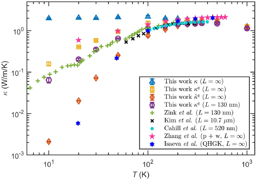
Figure 20: Evolution with temperature of the thermal conductivity of a-Si; comparison between simulation and experiment. “This work” here refers to Ref. Wang et al. (2023). Experimental references are to Zink et al. Zink et al. (2006), Kim et al. Kim et al. (2021), Cahill et al. Cahill et al. (1994), Zhang et al. Zhang et al. (2022) and Isaeva et al. Isaeva et al. (2019). Reprinted from Ref. Wang et al. (2023) with permission. Copyright (c) 2023 American Physical Society.

Properties of a-Si. While insight into the structure of a-Si is interesting on its own, for device applications we are also interested in emerging material properties, such as electronic band gap or thermal transport mechanism. To predict and understand these properties the key lies in finding the link between them and the underlying atomistic structure of the material. The number of MLP-driven studies of these properties in a-Si still lags behind the more developed literature on its atomistic structure, for the simple reason that the existence of reliable structural models precedes the calculation of properties, which must necessarily rely of the availability of those models. We expect to see rapid development in characterization and prediction of the properties of a-Si within large-scale atomistic simulation in the next few years. We mention here a recent example on thermal conductivity in a-Si. Wang et al. Wang et al. (2023) used an ANN-based NEP MLP Fan et al. (2021), implemented in the GPUMD code Fan et al. (2022), to perform highly efficient homogeneous non-equilibrium MD simulations of thermal transport in a-Si. This study has been able to closely reproduce the experimental evolution of the thermal conductivity of a-Si as a function of temperature and finite size (Fig. 20). This opens the door, in the near future, to simulating thermal properties of materials yet to be synthesized, with a high level of confidence in the accuracy of the computational results, in turn providing the basis for accelerated materials discovery and property-based materials design.

Table 1: List of some of the publicly available MLPs to simulate disordered C and Si, together with practical information. “Code” refers to the computer software which can be used to run a simulation with the corresponding MLP. GP stands for “general purpose”, i.e., it refers to an MLP which is not tailored exclusively to simulate a disordered phase but can be reliably used for that purpose. Whenever more than one version of the MLP exists, we give the reference to the latest one (i.e., on the table v2 refers to version 2 of a given MLP).

Material	Year	MLP flavor	Refs.	Code(s)
a-C	2017	GAP	Deringer and Csányi (2017)	QUIP, LAMMPS
C (GP)	2020	SNAP	Willman et al. (2020)	LAMMPS
a-C	2021 (v2)	GAP	Caro (2020c); Wang et al. (2022)	QUIP, LAMMPS, TurboGAP
C (GP)	2021	GAP	Muhli and Caro (2021); Muhli et al. (2021)	QUIP, LAMMPS, TurboGAP
C (GP)	2022 (v2)	GAP	Rowe et al. (2020); Csányi (2022)	QUIP, LAMMPS
a-C	2022	NEP	Fan et al. (2022); ref	GPUMD
C (GP)	2022	ACE	Qamar et al. (2022)	LAMMPS
Si (GP)	2018	GAP	Bartók et al. (2018); Csányi (2021)	QUIP, LAMMPS
Si (GP)	2021	GAP	Caro (2021)	QUIP, LAMMPS, TurboGAP
Si (GP)	2021	NEP	Fan et al. (2021); ref	GPUMD
a-Si:H	2022	GAP	Unruh et al. (2022)	QUIP, LAMMPS

Hydrogenated a-Si. While a-Si is an interesting material from a fundamental scientific perspective, as the prototypical amorphous semiconductor, hydrogenated a-Si (a-Si:H) is arguably more important from a technological point of view. a-Si:H is commonly used in solar cells, where the intentional doping with H heals the coordination defects that are present in undoped a-Si, improving material properties towards photovoltaic applications. Unfortunately, the introduction of additional chemical species makes the development of accurate MLPs more challenging, because of the larger configuration spaced spanned. At the same time, the CPU cost of an MLP calculation with multiple species is more expensive (“curse of dimensionality”) than for single species, with descriptor construction typically scaling between exponentially (worst-case scenario) and linearly (best-case scenario) with the number of species. For this reason there are comparatively few studies on a-Si:H or Si alloys compared to pure Si. On the other hand, thanks to recent developments in MLP technology, such as descriptor compression Darby et al. (2022), and the improved collective expertise gained by the community on how to generate good databases to train transferable MLPs, these multispecies force fields are starting to emerge. Here we mention in particular the recent effort by Unruh et al. to develop an a-Si:H GAP Unruh et al. (2022). The new Si-H GAP shows quantitative agreement with DFT and a significant improvement upon previously available classical (non-ML) force fields. This new MLP enabled the authors to model nanopores in a-Si:H. In the near future, either this force field or an extension combining its training database with existing and new ones may enable device-size simulation of c-Si/a-Si:H heterojuctions towards mitigating degradation mechanisms Jordan et al. (2017), of major technological importance for high-efficiency solar cells.

VI Available MLPs

Table 1 provides a non-comprehensive list of available MLPs able to simulate a-C and a-Si, together with their ML “flavor” and which code(s) they can be used with. These potentials are mostly of the GAP flavor, since the GAP community has been the most active at simulating a-C and a-Si among the different MLP developers and users base.

VII Summary and outlook

In this Topical Review we have introduced MLPs as powerful tools for the simulation of disordered materials at the atomic scale, making it possible to accurately study atomistic systems within sizes and time scales that were out of reach just a few years ago. We have discussed how these new tools have been used to shed light on important questions for understanding the structure of a-C and a-Si. MLPs have been used to elucidate the growth mechanism in diamondlike carbon and the high-pressure phase transformation from a-Si to a high-coordination metallic Si phase. MLPs have been used to study phase transitions at extreme thermodynamic conditions in carbon materials, and to understand the structure of nanoporous carbon, a material of increasing importance in battery research. These tools are being extended to more complicated systems, in particular H- and O-doped a-C and H-doped a-Si, enabling a further degree of realism in simulating these structurally complex materials. Furthermore, MLPs are being coupled to other ML approaches, including electronic-structure and spectroscopic signature prediction, improving the prospects for direct comparison and better integration between experiment and simulation. All in all, the future of atomistic modeling of disordered materials, also beyond a-C and a-Si, looks bright in the wake of MLPs. We should expect important breakthroughs in materials research in the years to come, brought about by these new powerful computational tools.