A hyper-parameterization method for comprehensive ocean models: Advection of the image point

Abstract

Idealized and comprehensive ocean models at low resolutions cannot reproduce nominally-resolved flow structures similar to those presented in the high-resolution solution. Although there are various underlying physical reasons for this, from the dynamical system point of view all these reasons manifest themselves as a low-resolution trajectory avoiding the phase space occupied by the reference solution (the high-resolution solution projected onto the coarse grid). In order to solve this problem, a set of hyper-parameterization methods has recently been proposed and successfully tested on idealized ocean models. In this work, for the first time we apply one of hyper-parameterization methods (Advection of the image point) to a comprehensive, rather than idealized, general circulation model of the North Atlantic.

The results show that the hyper-parameterization method significantly improves a non-eddy-resolving solution towards the reference eddy-resolving solution by reproducing both the large- and small-scale features of the Gulf Stream flow. The proposed method is much faster than even a single run of the coarse-grid ocean model, requires no modification of the model, and is easy to implement. Moreover, the method can take not only the reference solution as input data but also real measurements from different sources (drifters, weather stations, etc.), or combination of both. All this offers a great flexibility to ocean modellers working with mathematical models and/or measurements.

1 Introduction

The eddy parameterization problem (how to account for the effect of unresolved small scales onto the resolved large scales) is one of the most challenging problems in the ocean modelling, counting decades of active research. Despite a number of parameterizations (computationally affordable and physically justified mathematical models of unresolved processes) have been proposed to solve the problem (e.g., Gent and Mcwilliams, [12], Duan and Nadiga, [10], Frederiksen et al., [11], Mana and Zanna, [14], Cooper and Zanna, [4], Grooms et al., [13], Berloff, [1, 2, 3], Ryzhov et al., [16], Cotter et al., [5], Ryzhov et al., [17], Cotter et al., 2020a [6], Cotter et al., 2020b [7], Cotter et al., 2020c [8]), it remains largely unresolved. The main general point is that most of the parameterization approaches are physics-based rather than data-driven, and the former has obvious advantage of being valid in situation when the underlying physics changes. However, in the situation when physics-based parameterizations remain in their infancy, there is a great practicality in considering data-driven parameterizations, which can reproduce nominally-resolved flow structures within their obvious limitations. For example, for many research questions a computationally-cheap data-driven solution can replace a computationally-expensive dynamical ocean simulation in climate-type models and predictions. Advancing the hyper-parameterization approach, within broader context of data-driven parameterizations, provides the main motivation for our study, in which we continue the series of precursor works [18, 20, 19]. The main novelty is to adapt the methodology for fully comprehensive and realistic ocean models, and demonstrate its success with full confidence. In turn this paves the way for broad use of hyper-parameterizations across the ocean modelling community.

2 The method

In this work, we consider the method called “Advection of the image point”; it is called so, because the image point is advected by the flow in phase space. The method falls into the category of data-driven methods, and has been successfully tested on a multi-layer quasi-geostrophic model and showed promising results [18]. The method is based on the fact that the first-order ordinary differential equation

$$\mathbf{x}^{\prime}(t)=\mathbf{F}(\mathbf{x}),\quad\mathbf{x}\in\mathbb{R}^{n}$$ (1)

can be interpreted as a vector field $\mathbf{F}(\mathbf{x})$ in the phase space of equation (1). If $\mathbf{F}(\mathbf{x})$ is known, it can be used to advect the image point $\mathbf{x}$ in the phase space. Evolution of an image point can be described by the equation:

$$\mathbf{y}^{\prime}(t)=\frac{1}{N}\sum\limits_{i\in\mathcal{U}(\mathbf{y}(t))}\mathbf{F}(\mathbf{x}(t_{i}))+\eta\left(\frac{1}{M}\sum\limits_{i\in\mathcal{U}(\mathbf{y}(t))}\mathbf{x}(t_{i})-\mathbf{y}(t)\right),\quad\mathbf{y}(t_{0})=\mathbf{x}(t_{0})\,,$$ (2)

where $\mathcal{U}(\mathbf{y}(t))$ is a neighbourhood of solution $\mathbf{y}(t)$, and $i$ is the timestep of the reference solution $\mathbf{x}(t_{i})$. The neighbourhood is computed as the average over $N$ (and $M$ for the nudging term) nearest, in $l_{2}$ norm, to the solution $\mathbf{y}(t)$ points, and $\eta$ is the nudging strength; we will return to the choice of $N$, $M$, and $\eta$ in the next section; we refer to these parameters as hyper-parameters. The hyper-parameters can be set based on the chosen metric and available data. Getting a bit ahead, we report that in our case the neighbourhood consists of $N=15$ and $M=5$ points, and the nudging strength is $\eta=0.001$. Originally, the method was supposed to have the same size of the neighborhood for both the vector field $\mathbf{F}(\mathbf{x})$ and the nudging term (i.e., $N=M$). However, our experiments showed that using neighborhoods of different sizes can prevent the so-called build-up effect which we discuss later. We refer the reader to [18] for a more detailed discussion of the method.

3 Model configuration and numerical results

For the purpose of this study, we consider the Massachusetts Institute of Technology general circulation model (MITgcm) [15] in the North Atlantic configuration [20]. It is a 46-layer oceanic model coupled with an atmospheric boundary model [15, 9]. The coupled model is initially spun up for 5 years and then integrated for another 2 years. Although, for this work it is not essential that the initial state of the ocean circulation is in the statistically equilibrated regime. The model is integrated at two different horizontal resolutions ($1/12^{\circ}$ and $1/3^{\circ}$); the oceanic and atmospheric models are implemented with the same horizontal resolution. We refer to the $1/12^{\circ}$-solution projected onto the $1/3^{\circ}$-grid (Figure 1a) as the reference solution, and to the solution computed on the $1/3^{\circ}$-grid as the modelled solution (Figure 1c). The hyper-parameterized solution computed with equation (2) is presented in Figure 1b.

$t=1$ year

$t=2$ years

2-year average

(a)
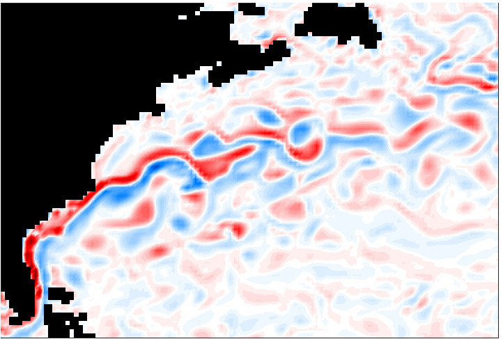
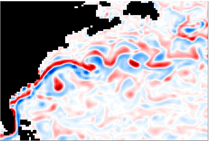
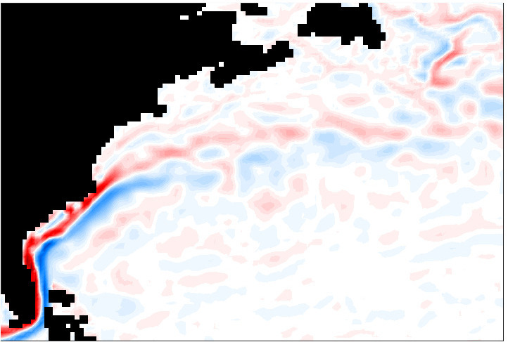
(b)
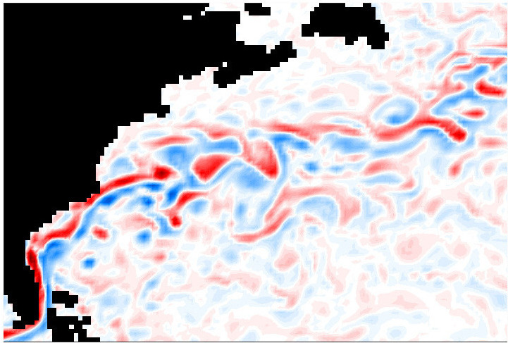
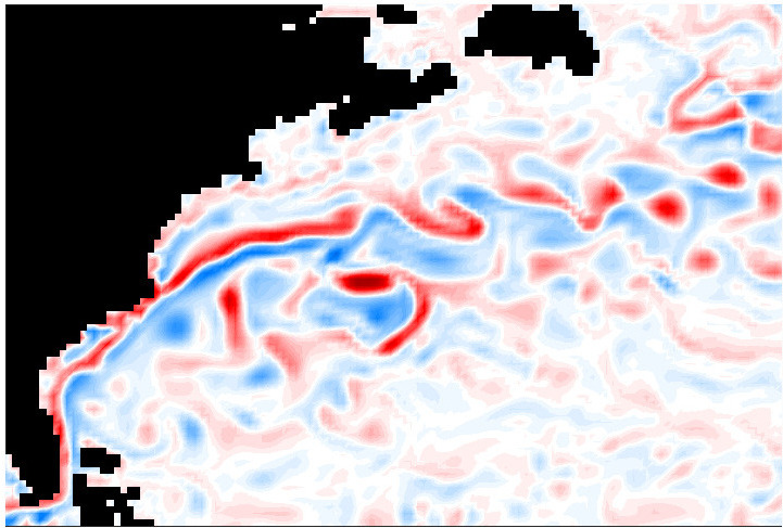
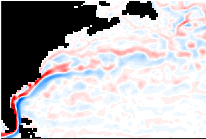
(c)

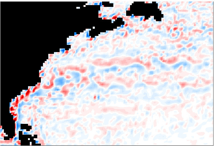
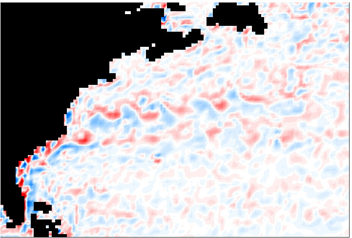
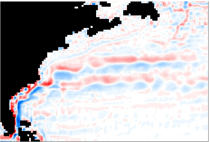
Figure 1: Shown are snapshots of the surface relative vorticity $\zeta=v_{x}-u_{y}$ [1/s] for (a) the reference solution (computed at horizontal resolution $1/12^{\circ}$ and then projected on the $1/3^{\circ}$-grid), (b) hyper-parameterized solution computed at horizontal resolution $1/3^{\circ}$ for $N=15$, $M=5$, $\eta=0.001$, (c) modelled solution computed at horizontal resolution $1/3^{\circ}$, and the 2-year time-average (last column). Snapshots are taken after 1 year (left column) and 2 years (middle column) of simulations. Note the modelled solution (c) fails to reproduce important large-scale (the Gulf Stream eastward jet extension) and small-scale (vortices) structures of the flow dynamics in both instantaneous and time-averaged fields.

As it follows from the results in Figure 1, the hyper-parameterized solution computed on the coarse grid (Figure 1b) reproduces both the large scales (the Gulf Stream flow) and small scales (vortices) of the reference solution (Figure 1a) in instantaneous and time-averaged fields, while the solution computed on the coarse grid without the hyper-parameterization (Figure 1c) leads to no Gulf Stream or small-scale flow features. We remark that the hyper-parameterized solution is a part of a 2-year simulation from which we use only the first year of the reference solution; over the second year model (2) runs on its own.

The hyper-parameterized solution with a bad choice of hyper-parameters $N$, $M$, $\eta$ (Figure 2) still reproduces both large- and small-scales flow features but only over the period in which the reference solution is available (it is one year in our case). After that the solution almost stops evolving and eventually settles to a constant in time field like the one in the middle plot of Figure 2. It can be seen from the time-mean over the second year (the right subplot in Figure 2), which is very similar to the snapshot taken at year 2 (middle subplot in Figure 2), thus showing that the solution evolution is stalled over the second year.

The build-up effect for the hyper-parameterized solution
$t=1$ year	$t=2$ years	Time-average over the second year

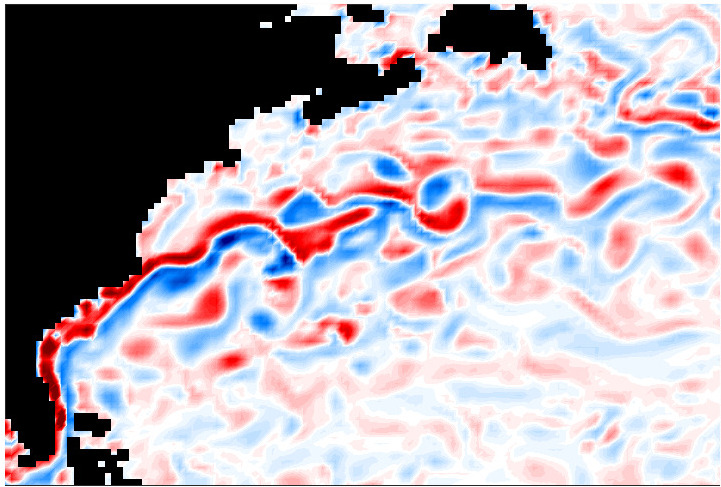
Figure 2: Shown are snapshots of the surface relative vorticity $\zeta=v_{x}-u_{y}$ [1/s] demonstrating the build-up effect for the hyper-parameterized solution computed at horizontal resolution $1/3^{\circ}$ for $N=M=5$, $\eta=0.001$. Snapshots are taken after 1 year (left column) and 2 years (middle column) of simulations.

The build-up effect and solution degradation. The lack of reference data for the hyper-parameterized model and/or bad choice of hyper-parameters can steer the trajectory to leave the reference phase space (the phase space occupied by the reference solution). This escape may result in a significant degradation of the hyper-parameterized solution and even lead to a numerical blow-up. We refer to this as the build-up effect, meaning that after a period of time, say $T$, the neighbourhood of the nearest points stalls (Figure 2), i.e. the points in the neighbourhood become the closest ones to the image point $\mathbf{y}(t)$ for $\forall t>T$ (in the present case $T=1$ year); therefore, the same points are used again and again during the integration of equation (2) thus driving the image point away from the reference phase space. In principle, building up numerical errors may terminate this runaway, and the solution can return back to the reference phase space region, but this is case dependent and should be kept in mind. However, if the return time is relatively long (longer than the characteristic time of the reference solution) then the flow dynamics can be seriously distorted over the period of the trajectory injection.

In order to prevent the build-up effect, one should properly set up the hyper-parameters $N$, $M$, and $\eta$. After some experiments we have found that $N=15$, $M=5$, and $\eta=0.001$ lead to no build-up effect (it is not necessarily the only choice, and other sets of hyper-parameters providing no build-up may exist). As an alternative, one can also change the algorithm on how to pickup points from the neighbourhood. It is worth noting that these experiments are very fast and computationally cheap, even relative to a single run of the coarse-grid model. We leave for the future work any further optimization of the image point advection algorithm.

The measure of goodness and evolution in phase space. The measure of goodness (i.e., the proximity of the modelled or parameterized solution to the reference one) in a given metric depends on the specific purpose. Our measure of goodness is how close the hyper-parameterized solution is to the reference phase space. We use this measure to allow the hyper-parameterized solution to evolve in the neighborhood of the reference phase space, since the failure of the coarse-grid model (blue dots in Figure 3) to reproduce large- and small-scale features of the flow dynamics is because it steers away from where it should be (black dots in Figure 3, i.e. the reference phase space). Measuring the proximity of individual trajectories in phase space is of no value, because small initial perturbations will grow exponentially due to the inherently chaotic dynamics.

(a)	(b)

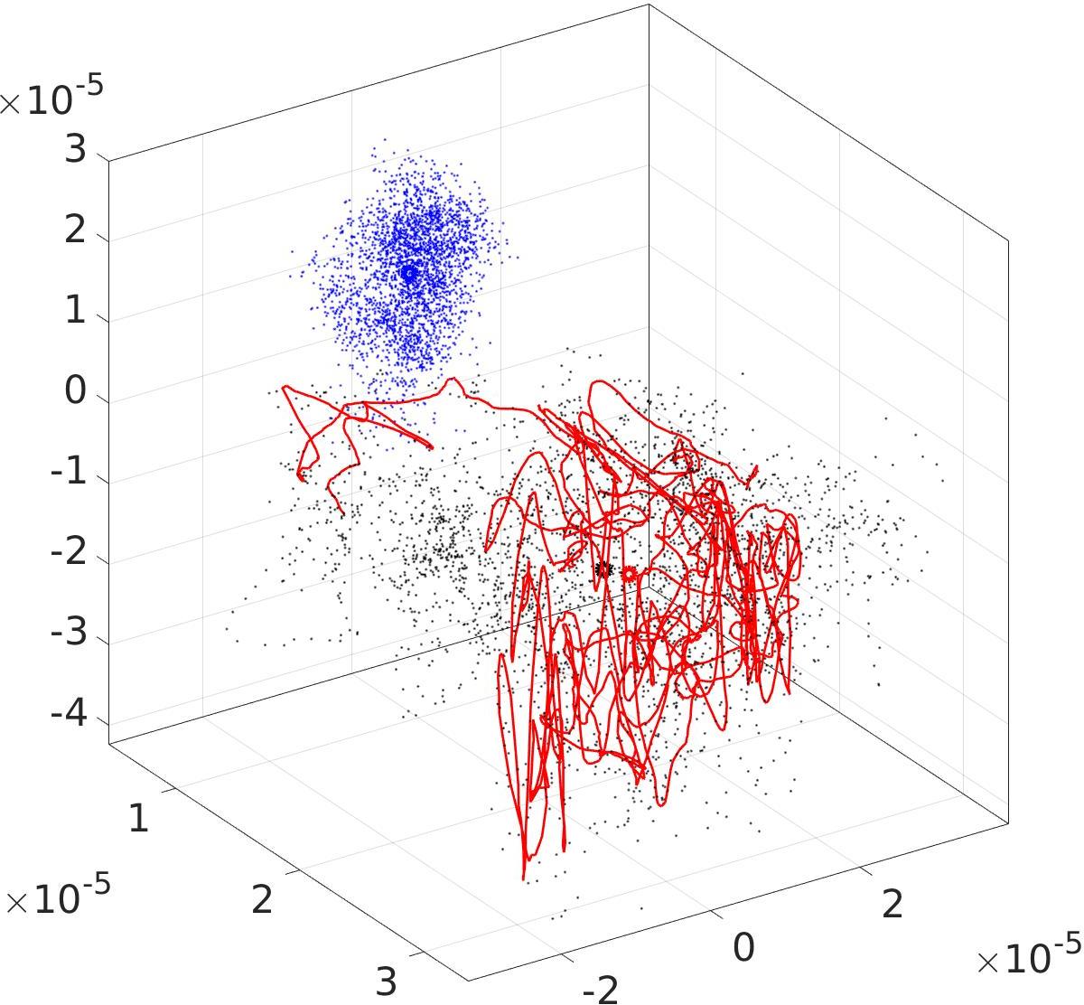
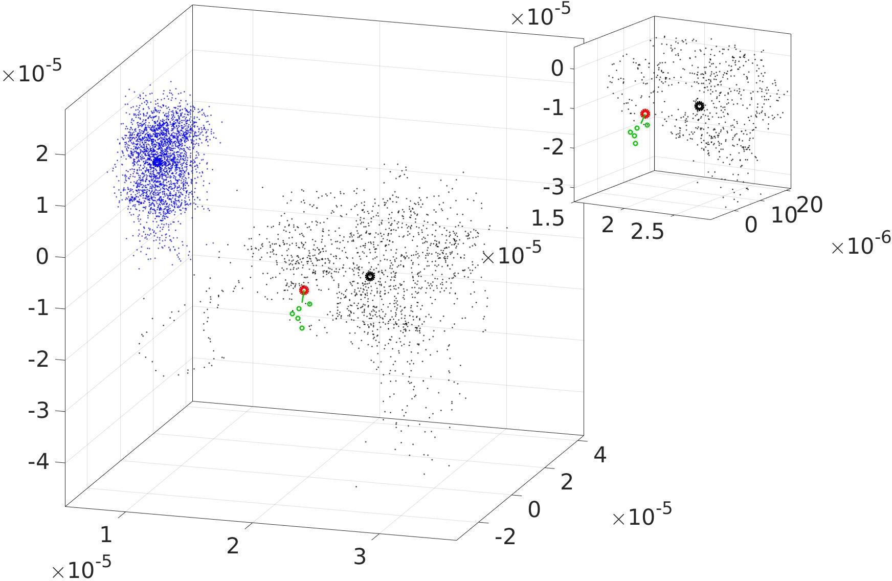
Figure 3: Shown is (a) 3D projection of the reference phase space (black dots), modelled phase space (blue dots), hyper-parameterized solution (red trajectory); in other words, we plot 3 random coordinates from the multi-dimensional phase space of surface relative vorticity, (b) build-up effect for the second year of the hyper-parameterized solution (short green line near the red circle) for $N=M=5$, and $\eta=0.001$; the green circles are those stalled five points in the neighborhood. The time-means for every solution are denoted by bold circles of corresponding colours.

The build-up effect is demonstrated in Figure 3b; the short green line near the time-mean over the second year (red circle) is the 1-year evolution of the hyper-parameterized solution affected by the bad choice of hyper-parameters, namely $N=M=5$, and $\eta=0.001$. Evolution of the Euclidean distance from the reference time mean (the time-mean of the reference solution) to the hyper-parameterized solution (Figure 4) shows that the hyper-parameterized solution affected by the build-up effect (green line) stops to evolve after one year (the period over which the reference solution is available). In this case, we observe no numerical blow-up as the solution quickly settles to a constant in time field. When the build-up effect is prevented, the hyper-parameterized solution (red line) continues to evolve with the reference phase space.

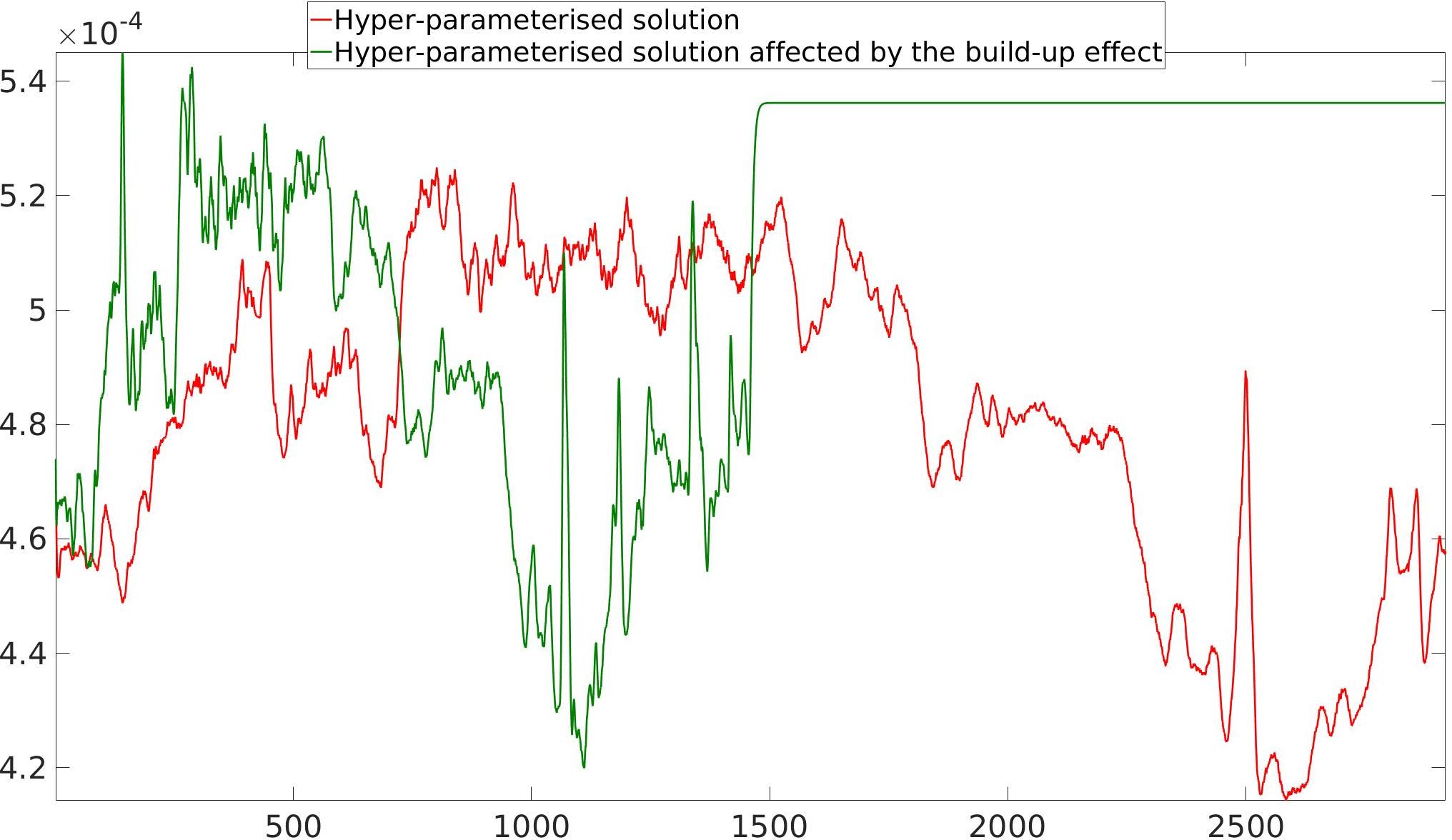
Figure 4: Shown is evolution of the Euclidean distance (vertical axis) from the reference two-year time-mean to the hyper-parameterized solution (red line) and to the hyper-parameterized solution affected by the build-up effect (green line). The horizontal axis shows the simulation time in time steps (6 hours in our case).

Coupled fields. Comprehensive ocean models have several prognostic fields (velocity, temperature, etc.), and a good choice of hyper-parameters ($N$, $M$, and $\eta$) for one field is not necessarily applicable to another. For example, $N=15$, $M=5$, and $\eta=0.001$ choice works well only for the relative vorticity. However, it leads to a build up for the coupled fields (relative vorticity and temperature, not shown). Thus, a set of hyper-parameters for a coupled case has to be found separately. Namely, for the coupled fields (relative vorticity and temperature) we have found that $N=18$ and $M=4$ remove the build up effect, hence, the hyper-parameterized solution is of high quality (Figure 5). The nudging strength in this case remains unchnged from the single relative vorticity case (Figure 1), $\eta=0.001$.

Surface relative vorticity
	$t=1$ year	$t=2$ years	2-year average

(a)
(b)

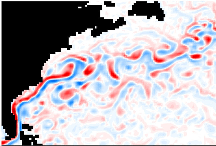
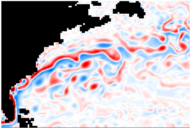
Sea surface temperature
	$t=1$ year	$t=2$ years	2-year average

(a)
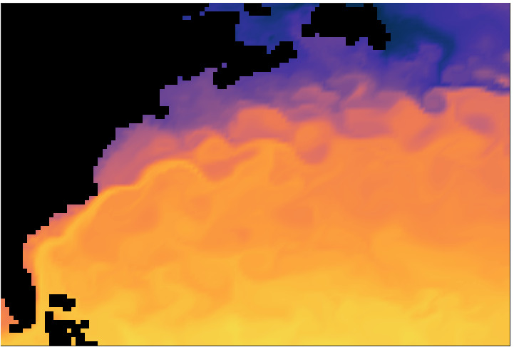
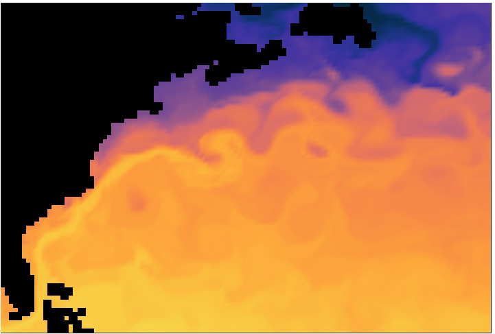
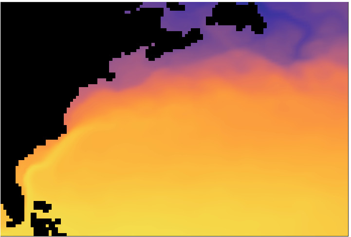
(b)

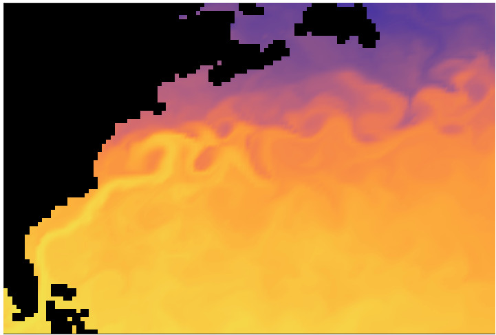
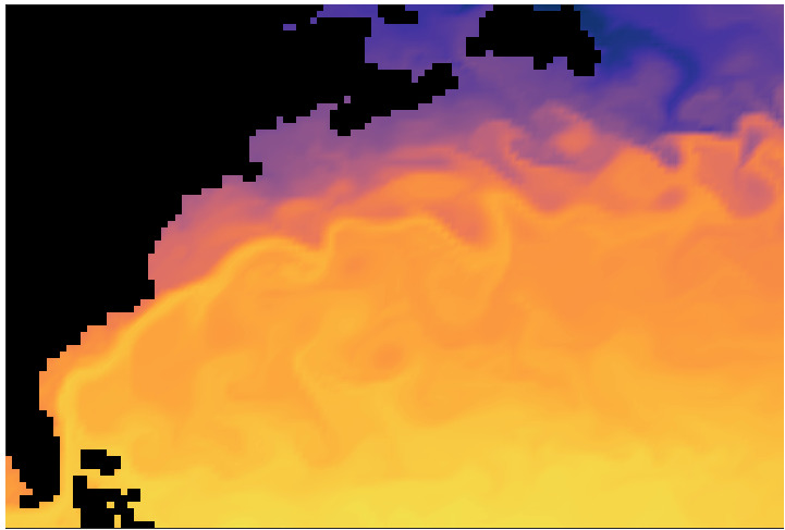
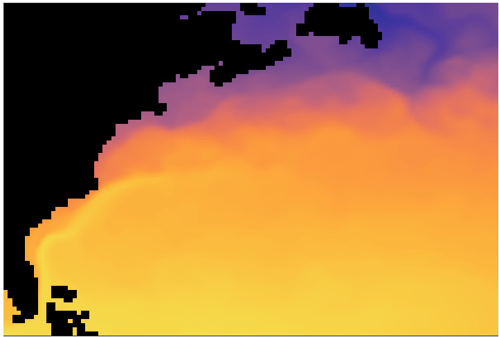
Figure 5: Shown are snapshots of the coupled fields (sea surface relative vorticity $\zeta=v_{x}-u_{y}$ [1/s] and surface temperature [${}^{\circ}{\rm C}$]) for (a) the reference solution (computed at horizontal resolution $1/12^{\circ}$ and then projected on the $1/3^{\circ}$-grid), (b) hyper-parameterized solution computed at horizontal resolution $1/3^{\circ}$ for $N=18$, $M=4$, $\eta=0.001$, and the 2-year time-average (last column). Snapshots are taken after 1 year (left column) and 2 years (middle column) of simulations. Note that the hyper-parameterized solution (b) reproduces both large- (the Gulf Stream) and small-scale (vortices) features of the flow dynamics in both fields.

This example of the coupled fields demonstrates that one should exercise caution when it comes to setting up the hyper-parameters. On the other hand, it also shows that the hyper-parameterization method works for coupled fields (even with huge differences between the fields, which is 7 orders of magnitude for the relative vorticity and temperature, see colorbars in Figure 5).

4 Conclusions and discussion

In this work we have applied the hyper-parameterization method “Advection of the image point” to the Massachusetts Institute of Technology general circulation model in the North Atlantic configuration and, thus, tested the method in a significantly more complicated setting, as compared to the earlier idealized-model tests. Our results show that the hyper-parameterization method significantly improves a non-eddy-resolving solution (on a $1/3^{\circ}$-grid) towards the reference eddy-resolving solution (on a $1/12^{\circ}$-grid and then projected onto the $1/3^{\circ}$-grid) for both single and coupled fields (even with large difference between the fields, it is 7 orders of magnitude in our case) by reproducing both the large-scale (the Gulf Stream eastward jet extension) and small-scale (vortices) flow features. It is important to note that the hyper-parameterization method reproduces both large- and small-scale flow features not only over the period for which the reference solution is available (1 year in our case), but also over the second year for which there is no reference data.

We have also explained the build-up effect and showed that a bad choice of hyper-parameters leads to the build-up effect, and eventually to a significant degradation of the hyper-parameterized solution. In the worst-case scenario, the build-up can lead to a numerical blow up (which we did not observe in our experiments though). The build-up can be avoided by a proper setup of hyper-parameters which we have found through a series of numerical experiments. In addition, the hyper-parameters have to be found separately for hyper-parameterizing single and coupled fields, as well as for different single fields (for instance, the hyper-parameters that work well for relative vorticity may not be optimal for temperature, and vice versa).

It is important to keep in mind that the proposed method is data-driven and, therefore, can suffer from lack of data as any data-driven method. The hyper-parameterization approach has other methods [20, 19] that can be used to reproduce effects of mesoscale oceanic eddies on the large-scale ocean circulation, but demonstration of their skills on the level of comprehensive models is left for the future. In other words, staying complimentary to the mainstream physics-based parameterization approach, we propose to work in phase space of the corresponding dynamical system and to interpret the lack of eddy effects as persistent tendency of phase space trajectories (representing the modelled solution) to escape the correct reference phase-space region.

The proposed method is much faster than even a single run of the coarse-grid ocean model, requires no modification of the model, and is easy to implement. The method can take as input data not only the reference solution but also real measurements from different sources (drifters, weather stations, etc.), or combination of both. All this offers a great flexibility not only to ocean modellers working with mathematical models but also to those working with measurements.

5 Acknowledgments

The authors thank The Leverhulme Trust for the support of this work through the grant RPG-2019-024.

References

- Berloff, [2015] Berloff, P. (2015). Dynamically consistent parameterization of mesoscale eddies. Part I: simple model. Ocean Model., 87:1–19.
- Berloff, [2016] Berloff, P. (2016). Dynamically consistent parameterization of mesoscale eddies. Part II: eddy fluxes and diffusivity from transient impulses. Fluids, 1:1–19.
- Berloff, [2018] Berloff, P. (2018). Dynamically consistent parameterization of mesoscale eddies. Part III: Deterministic approach. Ocean Model., 127:1–15.
- Cooper and Zanna, [2015] Cooper, F. and Zanna, L. (2015). Optimization of an idealised ocean model, stochastic parameterisation of sub-grid eddies. Ocean Model., 88:38–53.
- Cotter et al., [2019] Cotter, C., Crisan, D., Holm, D., Pan, W., and Shevchenko, I. (2019). Numerically modelling stochastic Lie transport in fluid dynamics. Multiscale Model. Simul., 17:192–232.
- [6] Cotter, C., Crisan, D., Holm, D., Pan, W., and Shevchenko, I. (2020a). A Particle Filter for Stochastic Advection by Lie Transport (SALT): A case study for the damped and forced incompressible 2D Euler equation. SIAM/ASA Journal on Uncertainty Quantification, 8:1446–1492.
- [7] Cotter, C., Crisan, D., Holm, D., Pan, W., and Shevchenko, I. (2020b). Data assimilation for a quasi-geostrophic model with circulation-preserving stochastic transport noise. Journal of Statistical Physics, 179:1186–1221.
- [8] Cotter, C., Crisan, D., Holm, D., Pan, W., and Shevchenko, I. (2020c). Modelling uncertainty using stochastic transport noise in a 2-layer quasi-geostrophic model. Foundations of Data Science, 2:173–205.
- Deremble et al., [2013] Deremble, B., Wienders, N., and Dewar, W. (2013). CheapAML: A simple, atmospheric boundary layer model for use in ocean-only model calculations. Mon. Wea. Rev., 141:809–821.
- Duan and Nadiga, [2007] Duan, J. and Nadiga, B. (2007). Stochastic parameterization for large eddy simulation of geophysical flows. Proc. Am. Math. Soc., 135:1187–1196.
- Frederiksen et al., [2012] Frederiksen, J., O’Kane, T., and Zidikheri, M. (2012). Stochastic subgrid parameterizations for atmospheric and oceanic flows. Phys. Scr., 85:068202.
- Gent and Mcwilliams, [1990] Gent, P. and Mcwilliams, J. (1990). Isopycnal mixing in ocean circulation models. J. Phys. Oceanogr., 20:150–155.
- Grooms et al., [2015] Grooms, I., Majda, A., and Smith, K. (2015). Stochastic superparametrization in a quasigeostrophic model of the Antarctic Circumpolar Current. Ocean Model., 85:1–15.
- Mana and Zanna, [2014] Mana, P. and Zanna, L. (2014). Toward a stochastic parameterization of ocean mesoscale eddies. Ocean Model., 79:1–20.
- Marshall et al., [1997] Marshall, J., Adcroft, A., Hill, C., Perelman, L., and Heisey, C. (1997). A finite-volume, incompressible Navier Stokes model for studies of the ocean on parallel computers. J. Geophys. Res., 102:5753–5766.
- Ryzhov et al., [2019] Ryzhov, E., Kondrashov, D., Agarwal, N., and Berloff, P. (2019). On data-driven augmentation of low-resolution ocean model dynamics. Ocean Model., 142:101464.
- Ryzhov et al., [2020] Ryzhov, E., Kondrashov, D., Agarwal, N., McWilliams, J., and Berloff, P. (2020). On data-driven induction of the low-frequency variability in a coarse-resolution ocean model. Ocean Model., 153:101664.
- Shevchenko and Berloff, [2021] Shevchenko, I. and Berloff, P. (2021). A method for preserving large-scale flow patterns in low-resolution ocean simulations. Ocean Model., 161:101795.
- [19] Shevchenko, I. and Berloff, P. (2022a). A method for preserving nominally-resolved flow patterns in low-resolution ocean simulations: Constrained dynamics. Ocean Model., 178:102098.
- [20] Shevchenko, I. and Berloff, P. (2022b). A method for preserving nominally-resolved flow patterns in low-resolution ocean simulations: Dynamical system reconstruction. Ocean Model., 161:101795.