Beat Transformer: Demixed Beat and Downbeat Tracking with Dilated Self-Attention

Abstract

We propose Beat Transformer, a novel Transformer encoder architecture for joint beat and downbeat tracking. Different from previous models that track beats solely based on the spectrogram of an audio mixture, our model deals with demixed spectrograms with multiple instrument channels. This is inspired by the fact that humans perceive metrical structures from richer musical contexts, such as chord progression and instrumentation. To this end, we develop a Transformer model with both time-wise attention and instrument-wise attention to capture deep-buried metrical cues. Moreover, our model adopts a novel dilated self-attention mechanism, which achieves powerful hierarchical modelling with only linear complexity. Experiments demonstrate a significant improvement in demixed beat tracking over the non-demixed version. Also, Beat Transformer achieves up to 4% point improvement in downbeat tracking accuracy over the TCN architectures. We further discover an interpretable attention pattern that mirrors our understanding of hierarchical metrical structures.

1 Introduction

Music audio beat and downbeat tracking, which aims to infer the very basic metrical structure of music, is a long-standing central topic in music information retrieval (MIR). A good beat estimation benefits various downstream MIR tasks, including transcription and structure analysis [1, 2, 3, 4, 5]. Moreover, beat tracking can be applied to human-computer interaction [6, 7], music therapy [8], and more scenes, as beats echo with human perceptual and motor sensitivity to musical rhythms.

We see significant progress in beat tracking with the development of deep neural networks. Current mainstream methods utilize temporal convolutional networks (TCNs) to extract frame-wise beat activations from an input spectrogram [9]. We further see successful efforts in boosting beat tracking performance, including phase-informed post-processing with dynamic Bayesian networks (DBNs) [10], multi-task learning for joint beat, downbeat and tempo estimation [11, 12, 13], and explicit beat phase modelling [14].

Recently, Transformer has demonstrated highly competitive performances over a range of MIR tasks [15, 16, 17, 18, 19, 20, 21]. In this paper, we propose Beat Transformer, a novel Transformer encoder architecture for joint beat and downbeat tracking. To better accommodate Transformer to our purpose, we introduce two extra inductive biases. Firstly, our model is constructed with short-windowed dilated self-attention. An exponentially increasing dilation rate enables our model to discern beats from non-beats in a hierarchical manner. With a fixed window size, our model maintains a linear complexity to the input sequence length.

Another inductive bias is demixed beat tracking. This strategy is inspired by the fact that human beat tracking is always accompanied by and enhanced by a deep understanding of the musical contexts. For example, the coordination of instruments enforces the progression of chords and bass notes, thus implying metrical accents, and such cues can be easily identified by human listeners. To capture this relation, we use Spleeter [22] to demix an input music piece into multiple instrument channels, and our model performs both time-wise and instrument-wise attention in alternate Transformer layers to excavate metrical cues.

We evaluate Beat Transformer on a wide range of beat- and downbeat-annotated datasets. Besides competing with state-of-the-art works, we present a thorough ablation study to illustrate the effectiveness of dilated self-attention and demixing. Moreover, our model learns highly interpretable representations. We demonstrate that our model can be interpreted as a learner over finite-state Markov chains, and we observe beat phase transition through visualization of the transition (attention) matrix.

In brief, the contributions of our paper are as follows:

• We propose Beat Transformer, a novel Transformer encoder architecture for joint beat and downbeat tracking in music audio.

• We devise dilated self-attention, which demonstrates powerful sequential modelling with linear complexity, potentially adaptable to more general MIR tasks.

• We make use of music demixing to complement and enhance beat tracking, shedding light on future MIR research towards universal music understanding.

2 Related Works

We review two topics related to our work: beat tracking, and Transformer. For beat tracking, we focus on its development with deep neural networks. For Transformer, we address its application in MIR. For more general review of both topics, we refer readers to [23] and [24], respectively.

2.1 Music Audio Beat Tracking

Beat tracking has been formulated as a two-stage sequential learning task. The first stage aims to determine the likelihood of beat presence, or beat activation, at each frame of an input spectrogram. The initial deep learning approach for this purpose was based on long short-term memory networks (LSTM) [25, 26]. To better pick up the beat sequence from raw model output, at the second stage, a dynamic Baysian network (DBN) is introduced to infer tempo and beat phase transition from beat activation [10].

The current mainstream methods substitute the LSTM with a TCN architecture [9, 12, 13, 14, 15]. Specifically, the convolutional kernels have a dilation rate exponential to the depth of layer. This hierarchical structure facilitates the network to model various scales, functionally similar to pooling, but maintains the same input and output size [27]. Besides architecture, another breakthrough of beat tracking is the formulation of multi-task learning [11, 12, 13, 14, 15]. Specifically, beat, downbeat, and tempo are strongly correlated metrical features. Sharing model weights among all three sub-tasks helps each to reach better convergence.

A recent trend of beat tracking is to deal with demixed music sources. Chiu et. al. leverages demixed drum and non-drum streams to enhance model adaptability to different drum source conditions [28, 29]. In fact, humans can track beats while switching their attention among different instrument parts. Hence the coordination of instrumental sources can be explored for useful metrical information.

In our work, we inherit the fashion of multi-task learning and the use of DBN, while proposing a novel Transformer encoder architecture to replace TCN. We formalize dilated self-attention [30, 31] for efficient modeling of long metrical structures. Moreover, we seek to enhance beat tracking by introducing instrumental attention among drum, piano, bass, vocal, and other demixed sources.

2.2 Transformer in MIR

Transformer has established itself de facto state-of-the-art in natural language and symbolic music domain. Recently, it has also demonstrated outstanding performance over audio-based MIR tasks, including music transcription [17, 18, 19], music tagging [20, 21], and other analysis [16]. For these tasks, a Transformer model is trained over short spectrogram clips typically of 2-5 seconds as a compromise to the quadratic complexity computing self-attention.

Transformer is first applied to beat tracking by Hung et. al. [15] using SpecTNT blocks [16]. For each SpecTNT block, a spectral Transformer encoder first aggregates spectral information at each time step, and then a temporal encoder exchanges information in time and pays attention to beat and downbeat positions. Such a time-frequency design makes an effective use of spectral features and achieves the state-of-the-art performance.

Our work is also a Transformer-based architecture that strives to enhance beat tracking with richer musical contexts. Instead of aggregating spectral features as in [15], we resort to demixed instrumental attention as a more explicit inductive bias to exploring spectral information. Our design of dilated self-attention is also a crucial step to accommodate Transformer to beat tracking. With only linear complexity, our model handles full-length songs at a time.

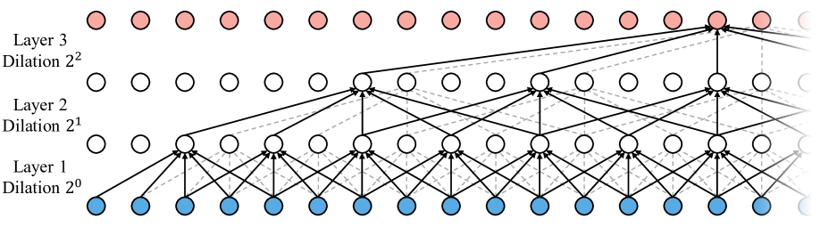
(a) Layer-wise view of dilated self-attention (Adapted from TCN structures [9, 27])

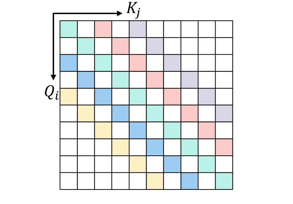
(b) Attention matrix view at layer 2

Figure 1: Illustration of dilated self-attention (with a non-causal short window of size 5) over a three-layer Transformer. Part (a) shows the hierarchical connectivity across layers, which shares the same pattern as TCN in [9]. Part (b) shows the attention matrix at layer 2, with colours indicating relative position. The white colour indicates unattainable positions.

3 Method

The core of our method is a Transformer encoder based on 1) dilated self-attention (DSA), and 2) demixed instrumental attention, to extract a framewise beat activation from input spectrograms. In this section, we first formalize DSA in Section 3.1. We then present our design of demixed beat tracking in Section 3.2. We further interpret our method with Markov chain properties in Section 3.3.

3.1 Dilated Self-Attention (DSA)

3.1.1 Background of Self-Attention (SA)

We first recall that, for vanilla Transformer layers, self-attention (SA) is computed via the scaled dot product:

$$\mathrm{Attention}(Q,K,V)=\mathrm{softmax}(\frac{QK^{\top}}{\sqrt{d_{\mathrm{f}}}})V,$$ (1)

where $Q_{1:T}$, $K_{1:T}$, $V_{1:T}\in\mathbb{R}^{T\times d_{\mathrm{f}}}$ are query, key, and value sequences, each linearly mapped from input $x_{1:T}$. $T$ is the sequence length, and $d_{\mathrm{f}}$ is the feature dimension.

The partial attention from position $i$ to $j$ is explicitly:

$$e_{ij}=\frac{Q_{i}K_{j}^{\top}}{\sqrt{d_{\mathrm{f}}}},$$ (2)

where $1\leq i,j\leq T$. Such computation leads to quadratic complexity $\mathcal{O}(T^{2})$ in terms of both time and space.

3.1.2 Dilated Self-Attention (DSA)

An illustration of DSA is shown in Figure 1. DSA is computed over a short window of size $l_{\mathrm{{win}}}=m+n+1$, where $m$ and $n$ are the length of non-causal and causal components of the window (in Figure 1, $m=n=2$). Each Transformer layer has a dilation rate $r\geqslant 1$, and $r$ increases exponentially as the layer goes deeper.

Formally, given $Q$, $K$, and $V\in\mathbb{R}^{T\times d_{\mathrm{f}}}$, DSA first computes Q-K attention by:

$$e_{ik}=\frac{Q_{i}K_{i+rk}^{\top}}{\sqrt{d_{\mathrm{f}}}},$$ (3)

where $1\leq i\leq T$ and $-m\leq k\leq n$. Specifically, $i+rk$ refers to the positions in $K_{1:T}$ that are attainable by $Q_{i}$ under the dilated window of rate $r$. When $i+rk$ exceeds the sequence range $[1,T]$, we fill $e_{ik}$ with $\mathtt{-inf}$.

Then, the Q-K attention $e_{ik}$ is normalized via softmax:

$$p_{ik}=\frac{\exp(e_{ik})}{\sum_{k=-m}^{n}\exp(e_{ik})}$$ (4)

The output of DSA is a sequence $z_{1:T}$, where $z_{i}$ is the weighted average of $V$ under the same dilated window:

$$z_{i}=\sum_{k=-m}^{n}p_{ik}(V_{i+rk})$$ (5)

We apply DSA with exponentially increasing dilation rates and relative positional embedding (RPE) [32] to a stack of Transformer layers. Each layer consists of two sub-layers: DSA, and a position-wise feed-forward layer. We place residual connections across each sub-layer and perform layer normalization [33] before each sub-layer.

3.1.3 Memory Efficient Implementation of DSA

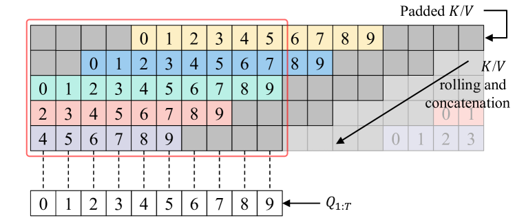
Figure 2: Illustration of efficient DSA implementation, with dilation rate $r=2$ and window size $l_{\mathrm{win}}=5$.

A straightforward implementation of DSA is to mask SA. Concretely, a square mask takes the same form as in Figure 1(b), where all uncolored positions are filled with $\mathtt{-inf}$, rendering a rather sparse attention matrix. This way, however, still requires quadratic complexity, because $e_{ij}$ is explicitly computed for all masked positions.

Our implementation takes a “rolling” strategy to eliminate redundant computation. As in Figure 2, $l_{\mathrm{win}}$ copies of $K_{1:T}$ sequences are padded and rolled along the time axis, and then concatenated on a new axis. In this way, each $Q_{i}$ sees $K_{j}$ directly and only at $j=i+rk$ for $-m\leq k\leq n$, which is exactly the coverage of the dilated window.

Formally, given $K_{1:T}\in\mathbb{R}^{T\times d_{\mathrm{f}}}$, dilation rate $r$, and window size $l_{\mathrm{win}}$, the rolling strategy takes three steps:

1. Pad $K_{1:T}$ with $\lfloor\frac{l_{\mathrm{win}}}{2}\rfloor\times r$ steps on both sides;

2. Make $l_{\mathrm{win}}$ copies of padded $K$. Starting from 0, each copy is cyclically rolled $r$ more steps;

3. Concatenate each copy along a new axis and retrieve the first $T$ steps. The output has shape $T\times l_{\mathrm{win}}\times d_{\mathrm{f}}$.

The same procedure applies to $V_{1:T}$ as well. In this way, computing DSA is essentially as simple as Equation (1). Here, instead of $Q,K,V\in\mathbb{R}^{T\times d_{\mathrm{f}}}$, we have $Q\in\mathbb{R}^{T\times 1\times d_{\mathrm{f}}}$ and $K$, $V\in\mathbb{R}^{T\times l_{\mathrm{win}}\times d_{\mathrm{f}}}$, with $T$ treated as a batch dimension. The computation complexity is $\mathcal{O}(T\times l_{\mathrm{win}})$, while $l_{\mathrm{win}}$ is fixed and small enough to be left uncounted.

3.2 Demixed Beat Tracking

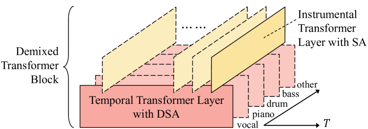
Figure 3: Demixed Transformer block. Two Transformer layers are stacked “orthogonally”, each handling time-wise dilated self-attention and instrument-wise self-attention.

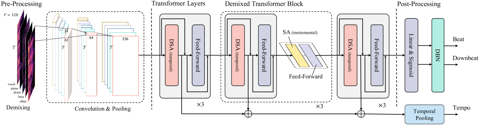
Figure 4: Beat Transformer architecture. For conciseness, layer normalization and dropout layers are not shown.

3.2.1 Demixed Transformer Block

We use Spleeter 5-stems model [22] to demix an input piece into spectrograms with $\left|C\right|$ instrument channels, where $C=\{\mathtt{vocal},\mathtt{piano},\mathtt{drum},\mathtt{bass},\mathtt{other}\}$. As shown in Figure 3, we stack two Transformer layers to perform time-wise and instrument-wise attention in turn. Let the input at layer $l$ be $x^{l}_{1:T,1:\left|C\right|}\in\mathbb{R}^{T\times\left|C\right|\times d_{\mathrm{f}}}$, a temporal Transformer layer (TTL) first takes $x_{1:T,c}^{l}$ for $1\leq c\leq\left|C\right|$:

$$x_{1:T,c}^{l+1}=\mathrm{TTL}(x_{1:T,c}^{l})$$ (6)

Then, an instrumental Transformer layer (ITL), on the orthogonal direction, takes $x_{t,1:\left|C\right|}^{l+1}$ for $1\leq t\leq T$:

$$x_{t,1:\left|C\right|}^{l+2}=\mathrm{ITL}(x_{t,1:\left|C\right|}^{l+1})$$ (7)

A TTL followed by ITL forms a demixed Transformer block. TTL consists of DSA as described in Section 3.1.2. For ITL, we use vanilla SA because there is only 5 instrument channels. As instruments are not sequentially ordered, we do not add any positional encoding to ITL.

Through demixed Transformer blocks, our model can capture the rhythmic evolution of each instrument, as well as the harmonic coordination among all instruments.

3.2.2 Partial Demix Augmentation

Spleeter may produce empty channels when a certain instrument does not present. To avoid potential effects of such a situations, we develop a partial demix strategy for data augmentation. Partial demix creates new stems by summing up existing instrument channels of a default 5-stem demixed input sample. For example, an augmented data sample may have three channels corresponding to $C^{\prime}=\{\mathtt{vocal\&piano},\mathtt{drum},\mathtt{bass\&other}\}$.

In our case, we randomly sum up $2$, $3$, or $4$ instrument channels of a 5-stem input with a probability $30\%$, $10\%$, and $10\%$ during training. In this way, our model is encouraged to pay attention to instrument-agnostic musical contents and thus is less affected by empty channels where no valid music content is present. As our augmentation strategy also adds to the demix diversity and the data quantity, we believe it brings general benefits to training as well.

3.3 Markov Chain Interpretation

In Equation (4), we formulate the attention matrix of DSA as $P=[p_{ij}]_{1\leq i,j\leq T}$, where $p_{ij}\geq 0$ if and only if $j=i+rk$ for $-m\leq k\leq n$. Here, $r$ is the dilation rate, and $m$, $n$ are components of the attention window. Moreover, $P$ satisfies $\sum_{j=1}^{T}p_{ij}=1$ for all $i$. Therefore, $P$ can be regarded as the transition matrix of a finite-state Markov chain, where each state is a position of the input sequence.

For a stack of temporal Transformer layers (TTL), where DSA is employed, layer $l$ essentially learns a unique one-step transition $P^{l}$, by which our model can attend to local neighbours covered by the attention window. Through $L$ layers, our model makes an $L$-step transition, during which it attends to global positions hierarchically. The overall $L$-step transition matrix $P^{(L)}$ satisfies:

$$P^{(L)}=\prod_{l=1}^{L}P^{l}$$ (8)

Note that $P^{l}$ itself is a rather sparse matrix (due to short attention window), while ${P^{(L)}}$ is densely connected. Its components $[p^{(L)}_{ij}]_{1\leq i,j\leq T}$ represent the hierarchical attention weights across the whole $L$ layers, which can tell us much richer attention patterns (more in Section 4.4).

		Beat Accuracy			Downbeat Accuracy
Dataset	Model	F-Measure	CMLt	AMLt	F-Measure	CMLt	AMLt
Ballroom	TCN+Demix	0.960	0.942	0.960	0.925	0.924	0.956
	Ours w/o Demix	0.968	0.946	0.965	0.930	0.925	0.963
	Ours w/o Aug.	0.967	0.949	0.967	0.928	0.931	0.958
	Ours	0.968	0.954	0.966	0.941	0.944	0.969
	Böck et al. [13]	0.962	0.947	0.961	0.916	0.913	0.960
	Hung et al. [15]	0.962	0.939	0.967	0.937	0.927	0.968
Hainsworth	TCN+Demix	0.887	0.827	0.918	0.739	0.708	0.861
	Ours w/o Demix	0.902	0.844	0.934	0.721	0.688	0.843
	Ours w/o Aug.	0.892	0.831	0.908	0.742	0.703	0.837
	Ours	0.902	0.842	0.918	0.748	0.712	0.841
	Böck et al. [13]	0.904	0.851	0.937	0.722	0.696	0.872
	Hung et al. [15]	0.877	0.862	0.915	0.748	0.738	0.870
Harmonix	TCN+Demix	0.954	0.903	0.956	0.901	0.866	0.923
	Ours w/o Demix	0.954	0.902	0.958	0.887	0.846	0.916
	Ours w/o Aug.	0.952	0.901	0.950	0.897	0.863	0.919
	Ours	0.954	0.905	0.957	0.898	0.863	0.919
	Böck et al. [13]∗	0.933	0.841	0.938	0.804	0.747	0.873
	Hung et al. [15]	0.953	0.939	0.959	0.908	0.872	0.928
SMC	TCN+Demix	0.596	0.455	0.625
	Ours w/o Demix	0.589	0.448	0.621
	Ours w/o Aug.	0.595	0.450	0.626
	Ours	0.596	0.456	0.635
	Böck et al. [13]	0.552	0.465	0.643
	Hung et al. [15]	0.605	0.514	0.663
GTZAN	TCN+Demix	0.873	0.780	0.907	0.700	0.646	0.842
	Ours w/o Demix	0.876	0.787	0.914	0.686	0.633	0.834
	Ours w/o Aug.	0.881	0.797	0.921	0.703	0.653	0.845
	Ours	0.885	0.800	0.922	0.714	0.665	0.844
	Böck et al. [13]	0.885	0.813	0.931	0.672	0.640	0.832
	Hung et al. [15]	0.887	0.812	0.920	0.756	0.715	0.881

Table 1: Testing results of beat and downbeat tracking under 8-fold cross-validation. GTZAN is unseen from training and held out for test only. Böck et. al. [13] on Harmonix is reproduced by [15], as indicated by the ^∗ symbol. We use underscore to denote best results comparing with our ablation models and use boldface to compare with state-of-the-art models.

3.4 Complete Architecture

A complete view of Beat Transformer is presented in Figure 4. The inputs are log-scaled spectrograms demixed by Spleeter, with $F=128$ mel-bins and $\left|C\right|=5$ instrument channels. Subject to Spleeter, our frame rate is $43.07$ fps and the frequency range is up to 11 kHz. We then use three 2D convolutional layers, shared by each demixed channel, as a front-end feature extractor. The convolutional design is the same as in [13] except that we employ more filters to reach feature dimension $d_{\mathrm{model}}=256$.

Beat Transformer comprises 9 temporal Transformer layers (TTL) with DSA. Each TTL has 8 attention heads with window size $l_{\mathrm{win}}=5$, four of which have skewed window ranges, where $m=0,1,3,4$, respectively, and $n=4-m$. The dilation rate grows exponentially from $2^{0}$ to $2^{8}$, stretching to a receptive field of $47.51$ seconds. Among the 9 TTLs, the middle three are expanded to demixed Transformer blocks by interleaving ITLs. We found it sufficient to perform instrumental attention only in the middle layers, which has a proper scale of $1$-$5$ seconds. Each Transformer layer has 8 heads ($d_{\mathrm{f}}=32$) followed by a feed-forward layer with hidden dimension $d_{\mathrm{ff}}=1024$.

We sum up the instrument channels of the output of the last Transformer layer and obtain a frame-wise beat representation of shape $T\times d_{\mathrm{model}}$. Following multi-task learning practice [11, 12, 13, 14], we use a linear layer to map the representation to beat and downbeat activations respectively, and add a regularization branch predicting global tempo via “skip connections” [12]. We apply DBN in Madmom package [34] as the post-processor to pick up the beat and downbeat sequence from raw activations. For DBN parameters, we set $\mathtt{observation\_lambda}=6$, $\mathtt{transition\_lambda}=100$, and $\mathtt{threshold}=0.2$.

4 Experiments

4.1 Datasets

We utilize a total of 7 datasets for model training and evaluation: Ballroom [35, 36], Hainsworth [37], RWC Popular [38], Harmonix [39], Carnetic [40], SMC [41], and GTZAN [42, 43]. We acquire Harmonix in mel-spectrogram and invert each piece to audio using Griffin-Lim Algorithm [44, 45] with Librosa package [46]. Following convention, we leave GTZAN for testing only and use the other datasets in 8-fold cross validation [11, 12, 13].

4.2 Training

Our model is supervised in a multi-task learning fashion, where beat, downbeat, and tempo are predicted jointly [13]. Beat and downbeat annotations are each represented as a 1D binary sequence that indicates beat ($1$) and non-beat ($0$) states at each input frame. Following [13], we widen beat and downbeat states to $\pm 2$ neighbours of annotated frames with weights $0.5$ and $0.25$. Following [12], we derive tempo target from beat annotation for the tempo prediction branch. We found the use of tempo branch generally beneficial to beat tracking, as it may serve as a regularization term that helps reaching better convergence.

For training, we combine the binary cross entropy loss over beat, downbeat, and tempo by weighing them equally. We use a batch size of 1 to train on whole sequences with different lengths. For excessively long songs, we split them into 3-minute (8k-frame) clips. We apply RAdam [47] plus Lookahead [48] optimizer with an initial learning rate of $1\mathrm{e}{-3}$, which is reduced by a factor of 5 whenever the validation loss gets stuck for 2 epochs before being capped at a minimum value of $1\mathrm{e}{-7}$. We use dropout [49] with rate $0.5$ for the tempo branch and $0.1$ for other parts of the network. We apply partial demix augmentation described in Section 3.2.2 as the only means of data augmentation. Our model has 9.29M trainable parameters and is trained with an RTX-A5000-24GB GPU. Each training fold generally takes 20 epochs (in 11 hours) to fully converge.

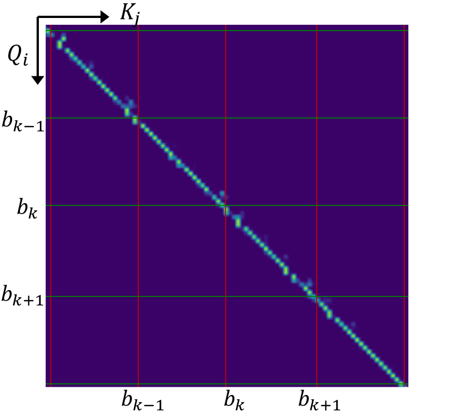
(a) ${P^{(1)}}$ lower scale

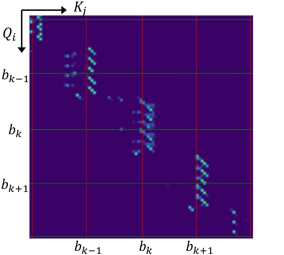
(b) ${P^{(3)}}$ beat scale

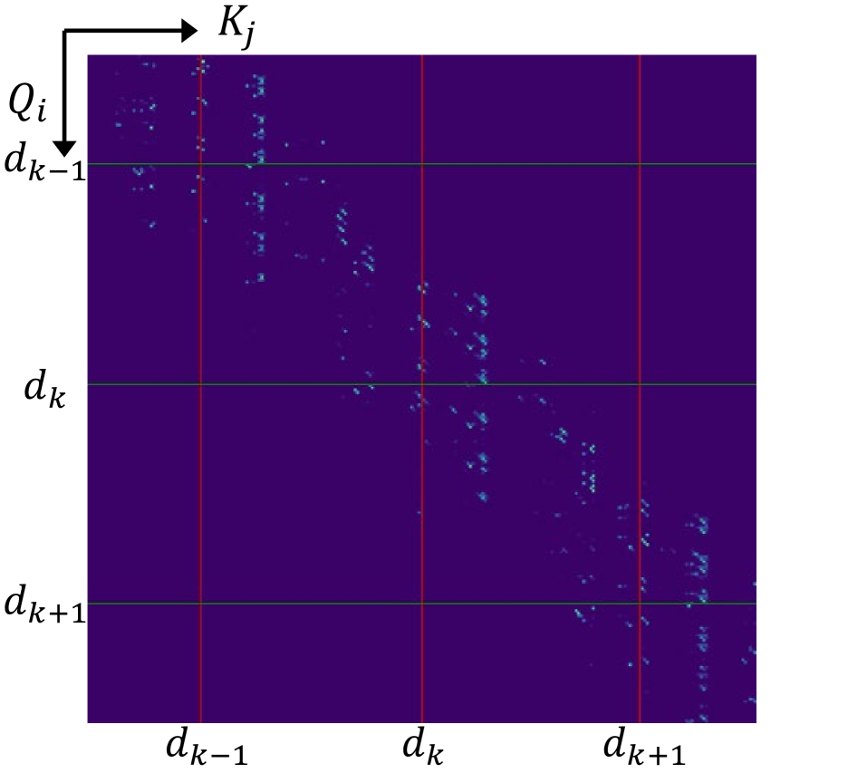
(c) ${P^{(5)}}$ downbeat scale

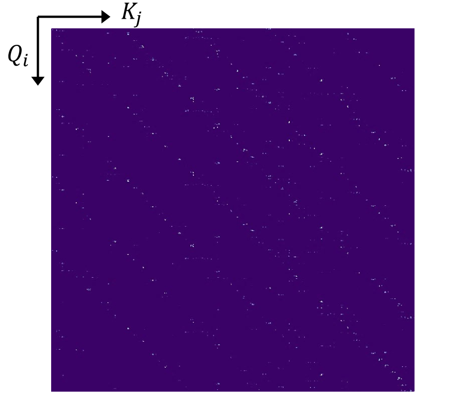
(d) ${P^{(9)}}$ higher scale

Figure 5: Visualization of temporal attention matrix based on the product rule in Equation (8) for $L$-step transition on a Markov chain. $L=1,3,5,$ and $9$ from part (a) to (d), which model different hierarchies of the metrical structure.

4.3 Evaluation

4.3.1 Baseline Methods

We first compare three ablation models to validate our module design. The first ablation model is Ours trained without partial demix augmentation (Ours w/o Aug.). The second model removes all ITL layers and tracks beat with a single channel of non-demixed mixture (Ours w/o Demix). The last model replaces each TTL layer with a TCN layer [13] of the same dilation rate (TCN+Demix). We implement TCN layers following [23] while setting the input and output shape to be the same as our model. The resulting model yields a comparable amount of 10.25M parameters and is trained without augmentation.

In addition, we compare our model with two recent works that have achieved state-of-the-art performance. Specifically, Böck et al. [13] is based on TCN architectures and Hung et al. [15] is based on SpecTNT.

4.3.2 Results and Discussion

In Table 1, we first observe Ours w/o Aug. yields generally better performance than TCN+Demix, especially on the unseen GTZAN dataset. As both models share a comparable amount of parameters, this result demonstrates the capability of Transformer (DSA) versus TCN (dilated convolution), which also corroborates with previous findings on Transformer’s comparability to convolution on general tasks [50, 51, 52]. Considering that Transformer is notoriously data-inefficient to train, it is remarkable that our model is well-trained with limited data without augmentation. We owe this merit to DSA, which not only prevents redundant computation but also makes musical sense in terms of the hierarchical structure of music metrical modelling.

Comparing Ours w/o Demix to Ours w/o Aug., while both models are highly competitive in beat tracking, the latter demonstrates more superiority in downbeat tracking. Downbeat tracking is generally more difficult than beat tracking because it is involved with deeper musical knowledge, such as chord and bass progression, behind the apparent spectrogram energy. In our model, the instrumental attention captures the instrumental coordination as hints to the harmonic cues that are orthogonal to the temporal axis, and thus acquires better metrical modelling.

Comparing Ours w/o Aug. to Ours, we observe a consistent improvement across datasets brought by partial demix augmentation, which indicates the general usefulness of this augmentation strategy to model training.

Compared to state-of-the-art models, our improvement in downbeat accuracy is more significant than that in beat accuracy. On the test-only GTZAN dataset, we obtain 4% point gain in F-measure over Böck et al. [13] in downbeat tracking. Compared to Hung et al. [15], which is also based on Transformer, our model can be more flexibly trained (owing to the efficient DSA mechanism) on a 24GB GPU in contrast to four 32GB GPUs reported in [15].

4.4 Attention Matrix Visualization

We visualize the attention matrix that our model learns by interpreting it as a multi-step Markov transition matrix as defined in Equation (8). Specifically, the $L$-step matrix is the product of $L$ one-step matrices through $L$ layers. Here we only consider TTLs with dilated self-attention, as ITLs work on an orthogonal axis. Figure 5 shows the attention matrix $P^{(L)}$ for $L=1,3,5,$ and $9$ of the $\mathtt{drum}$ channel, inferred from the piece $\mathtt{hiphop.00090}$ chosen from GTZAN.

Figure 5(a) shows a one-step transition. Each position $Q_{i}$ can only attend to its neighbours covered by the attention window. Still, we observe that beat positions (denoted by $b_{k}$) are likely to get more attention. In Figure 5(b) where we step to the beat scale, most attention spots are aligned with beats. Moreover, we observe that the attention at $b_{k}$ is typically prolonged after $Q_{i}$ leaves $b_{k}$, and is formed before $Q_{i}$ reaches $b_{k}$ for every $k$. This means that our model learns to transition its attention from the offbeat phase following the last beat to the upbeat phase preceding the next beat. Figure 5(c) further stretches the view to the downbeat scale, and we can see similar patterns aligned with downbeat positions (denoted by $d_{k}$). Finally, in Figure 5(d), the attention reaches further positions and displays a structural pattern.

The above visualization demonstrates the inner logic that our model exploits for beat and downbeat tracking. We see that our model gathers information from both local and global scales with an organized hierarchy.

5 Conclusion

In conclusion, we contribute a novel Transformer architecture for audio beat and downbeat tracking. The main novelty lies first in our design of dilated self-attention, which brings down the computation complexity of Transformer from quadratic to linear level. In addition, we successfully enhance beat and downbeat tracking by utilizing off-the-shelf progress in music demixing. Our model not only captures deeper harmonic cues for better metrical inference but also discerns beat and downbeat in a visualizable hierarchical manner. Our model is efficient, interpretable, and potentially generalizable with highly competitive sequential modelling power. We hope our model encourages future MIR research toward universal music understanding.

References

- [1] A. Holzapfel and E. Benetos, “The sousta corpus: Beat-informed automatic transcription of traditional dance tunes,” in Proceedings of the 17th International Society for Music Information Retrieval Conference, ISMIR, 2016, pp. 531–537.
- [2] G. Shibata, R. Nishikimi, and K. Yoshii, “Music structure analysis based on an LSTM-HSMM hybrid model,” in Proceedings of the 21th International Society for Music Information Retrieval Conference, ISMIR, 2020, pp. 23–29.
- [3] R. Nishikimi, E. Nakamura, M. Goto, K. Itoyama, and K. Yoshii, “Bayesian singing transcription based on a hierarchical generative model of keys, musical notes, and F0 trajectories,” IEEE ACM Transactions on Audio, Speech, and Language Processing, vol. 28, pp. 1678–1691, 2020.
- [4] R. Ishizuka, R. Nishikimi, and K. Yoshii, “Global structure-aware drum transcription based on self-attention mechanisms,” Signals, vol. 2, no. 3, pp. 508–526, 2021.
- [5] C. Donahue and P. Liang, “Sheet sage: Lead sheets from music audio,” 2021, Late Breaking Demo in the 22nd International Society for Music Information Retrieval Conference, ISMIR. [Online]. Available: https://archives.ismir.net/ismir2021/latebreaking/000049.pdf
- [6] T. Bi, P. Fankhauser, D. Bellicoso, and M. Hutter, “Real-time dance generation to music for a legged robot,” in 2018 IEEE/RSJ International Conference on Intelligent Robots and Systems, IROS. IEEE, 2018, pp. 1038–1044.
- [7] K. Yamamoto, “Human-in-the-loop adaptation for interactive musical beat tracking,” in Proceedings of the 22nd International Society for Music Information Retrieval Conference, ISMIR, 2021, pp. 794–801.
- [8] Z. Cai, R. J. Ellis, Z. Duan, H. Lu, and Y. Wang, “Basic evaluation of auditory temporal stability (beats): A novel rationale and implementation,” in Proceedings of the 14th International Society for Music Information Retrieval Conference, ISMIR, 2013, pp. 541–546.
- [9] E. P. MatthewDavies and S. Böck, “Temporal convolutional networks for musical audio beat tracking,” in 27th European Signal Processing Conference, EUSIPCO. IEEE, 2019, pp. 1–5.
- [10] F. Krebs, S. Böck, and G. Widmer, “An efficient state-space model for joint tempo and meter tracking,” in Proceedings of the 16th International Society for Music Information Retrieval Conference, ISMIR, 2015, pp. 72–78.
- [11] S. Böck, F. Krebs, and G. Widmer, “Joint beat and downbeat tracking with recurrent neural networks,” in Proceedings of the 17th International Society for Music Information Retrieval Conference, ISMIR, 2016, pp. 255–261.
- [12] S. Böck, M. E. P. Davies, and P. Knees, “Multi-task learning of tempo and beat: Learning one to improve the other,” in Proceedings of the 20th International Society for Music Information Retrieval Conference, ISMIR, 2019, pp. 486–493.
- [13] S. Böck and M. E. P. Davies, “Deconstruct, analyse, reconstruct: How to improve tempo, beat, and downbeat estimation,” in Proceedings of the 21th International Society for Music Information Retrieval Conference, ISMIR, 2020, pp. 574–582.
- [14] T. Oyama, R. Ishizuka, and K. Yoshii, “Phase-aware joint beat and downbeat estimation based on periodicity of metrical structure,” in Proceedings of the 22nd International Society for Music Information Retrieval Conference, ISMIR, 2021, pp. 493–499.
- [15] Y. Hung, J. Wang, X. Song, W. T. Lu, and M. Won, “Modeling beats and downbeats with a time-frequency transformer,” in IEEE International Conference on Acoustics, Speech and Signal Processing, ICASSP. IEEE, 2022, pp. 401–405.
- [16] W.-T. Lu, J.-C. Wang, M. Won, K. Choi, and X. Song, “SpecTNT: A time-frequency transformer for music audio,” in Proceedings of the 22nd International Society for Music Information Retrieval Conference, ISMIR, 2021, pp. 396–403.
- [17] C. Hawthorne, I. Simon, R. Swavely, E. Manilow, and J. Engel, “Sequence-to-sequence piano transcription with transformers,” in Proceedings of the 22nd International Society for Music Information Retrieval Conference, ISMIR, 2021, pp. 246–253.
- [18] L. Ou, Z. Guo, E. Benetos, J. Han, and Y. Wang, “Exploring transformer’s potential on automatic piano transcription,” in IEEE International Conference on Acoustics, Speech and Signal Processing, ICASSP. IEEE, 2022, pp. 776–780.
- [19] J. Gardner, I. Simon, E. Manilow, C. Hawthorne, and J. H. Engel, “MT3: multi-task multitrack music transcription,” in The Tenth International Conference on Learning Representations, ICLR. OpenReview.net, 2022.
- [20] M. Won, S. Chun, and X. Serra, “Toward interpretable music tagging with self-attention,” arXiv preprint arXiv:1906.04972, 2019.
- [21] M. Won, K. Choi, and X. Serra, “Semi-supervised music tagging transformer,” in Proceedings of the 22nd International Society for Music Information Retrieval Conference, ISMIR, 2021, pp. 769–776.
- [22] R. Hennequin, A. Khlif, F. Voituret, and M. Moussallam, “Spleeter: a fast and efficient music source separation tool with pre-trained models,” Journal of Open Source Software, vol. 5, no. 50, p. 2154, 2020, deezer Research. [Online]. Available: https://doi.org/10.21105/joss.02154
- [23] M. E. Davies, S. Böck, and M. Fuentes, Tempo, Beat and Downbeat Estimation, 2021. [Online]. Available: https://tempobeatdownbeat.github.io/tutorial/intro.html
- [24] T. Lin, Y. Wang, X. Liu, and X. Qiu, “A survey of transformers,” arXiv preprint arXiv:2106.04554, 2021.
- [25] S. Böck and M. Schedl, “Enhanced beat tracking with context-aware neural networks,” in Proceedings of the 14th International Conference on Digital Audio Effects, DAFx, 2011, pp. 135–139.
- [26] S. Böck, F. Krebs, and G. Widmer, “A multi-model approach to beat tracking considering heterogeneous music styles,” in Proceedings of the 15th International Society for Music Information Retrieval Conference, ISMIR, 2014, pp. 603–608.
- [27] A. van den Oord, S. Dieleman, H. Zen, K. Simonyan, O. Vinyals, A. Graves, N. Kalchbrenner, A. W. Senior, and K. Kavukcuoglu, “Wavenet: A generative model for raw audio,” in The 9th ISCA Speech Synthesis Workshop. ISCA, 2016, p. 125.
- [28] C. Chiu, J. Ching, W. Hsiao, Y. Chen, A. W. Su, and Y. Yang, “Source separation-based data augmentation for improved joint beat and downbeat tracking,” in 29th European Signal Processing Conference, EUSIPCO. IEEE, 2021, pp. 391–395.
- [29] C. Chiu, A. W. Su, and Y. Yang, “Drum-aware ensemble architecture for improved joint musical beat and downbeat tracking,” IEEE Signal Processing Letters, vol. 28, pp. 1100–1104, 2021.
- [30] R. Dai, S. Das, L. Minciullo, L. Garattoni, G. Francesca, and F. Brémond, “PDAN: pyramid dilated attention network for action detection,” in IEEE Winter Conference on Applications of Computer Vision, WACV. IEEE, 2021, pp. 2969–2978.
- [31] N. Moritz, T. Hori, and J. L. Roux, “Capturing multi-resolution context by dilated self-attention,” in IEEE International Conference on Acoustics, Speech and Signal Processing, ICASSP. IEEE, 2021, pp. 5869–5873.
- [32] P. Shaw, J. Uszkoreit, and A. Vaswani, “Self-attention with relative position representations,” in Proceedings of the 2018 Conference of the North American Chapter of the Association for Computational Linguistics: Human Language Technologies, NAACL-HLT, Volume 2. Association for Computational Linguistics, 2018, pp. 464–468.
- [33] J. L. Ba, J. R. Kiros, and G. E. Hinton, “Layer normalization,” arXiv preprint arXiv:1607.06450, 2016.
- [34] S. Böck, F. Korzeniowski, J. Schlüter, F. Krebs, and G. Widmer, “madmom: A new python audio and music signal processing library,” in Proceedings of the 2016 ACM Conference on Multimedia Conference, MM. ACM, 2016, pp. 1174–1178.
- [35] F. Gouyon, A. Klapuri, S. Dixon, M. Alonso, G. Tzanetakis, C. Uhle, and P. Cano, “An experimental comparison of audio tempo induction algorithms,” IEEE Transactions on Audio, Speech, and Language Processing, vol. 14, no. 5, pp. 1832–1844, 2006.
- [36] F. Krebs, S. Böck, and G. Widmer, “Rhythmic pattern modeling for beat and downbeat tracking in musical audio,” in Proceedings of the 14th International Society for Music Information Retrieval Conference, ISMIR, 2013, pp. 227–232.
- [37] S. W. Hainsworth and M. D. Macleod, “Particle filtering applied to musical tempo tracking,” EURASIP Journal on Advances in Signal Processing, vol. 2004, no. 15, pp. 1–11, 2004.
- [38] M. Goto, H. Hashiguchi, T. Nishimura, and R. Oka, “RWC music database: Popular, classical and jazz music databases,” in ISMIR 2002, 3rd International Conference on Music Information Retrieval, 2002.
- [39] O. Nieto, M. McCallum, M. E. P. Davies, A. Robertson, A. M. Stark, and E. Egozy, “The harmonix set: Beats, downbeats, and functional segment annotations of western popular music,” in Proceedings of the 20th International Society for Music Information Retrieval Conference, ISMIR, 2019, pp. 565–572.
- [40] A. Srinivasamurthy and X. Serra, “A supervised approach to hierarchical metrical cycle tracking from audio music recordings,” in IEEE International Conference on Acoustics, Speech and Signal Processing, ICASSP. IEEE, 2014, pp. 5217–5221.
- [41] A. Holzapfel, M. E. P. Davies, J. R. Zapata, J. L. Oliveira, and F. Gouyon, “Selective sampling for beat tracking evaluation,” IEEE Transactions on Speech and Audio Processing, vol. 20, no. 9, pp. 2539–2548, 2012.
- [42] G. Tzanetakis and P. R. Cook, “Musical genre classification of audio signals,” IEEE Transactions on Speech and Audio Processing, vol. 10, no. 5, pp. 293–302, 2002.
- [43] U. Marchand and G. Peeters, “Swing ratio estimation,” in Proceedings of the 18th International Conference on Digital Audio Effects, DAFx, 2015.
- [44] D. Griffin and J. Lim, “Signal estimation from modified short-time fourier transform,” IEEE Transactions on acoustics, speech, and signal processing, vol. 32, no. 2, pp. 236–243, 1984.
- [45] N. Perraudin, P. Balázs, and P. L. Søndergaard, “A fast griffin-lim algorithm,” in IEEE Workshop on Applications of Signal Processing to Audio and Acoustics, WASPAA. IEEE, 2013, pp. 1–4.
- [46] B. McFee, C. Raffel, D. Liang, D. P. Ellis, M. McVicar, E. Battenberg, and O. Nieto, “librosa: Audio and music signal analysis in python,” in Proceedings of the 14th python in science conference, vol. 8. Citeseer, 2015, pp. 18–25.
- [47] L. Liu, H. Jiang, P. He, W. Chen, X. Liu, J. Gao, and J. Han, “On the variance of the adaptive learning rate and beyond,” in 8th International Conference on Learning Representations, ICLR. OpenReview.net, 2020.
- [48] M. R. Zhang, J. Lucas, J. Ba, and G. E. Hinton, “Lookahead optimizer: k steps forward, 1 step back,” in Advances in Neural Information Processing Systems 32: Annual Conference on Neural Information Processing Systems, NeurIPS, 2019, pp. 9593–9604.
- [49] N. Srivastava, G. E. Hinton, A. Krizhevsky, I. Sutskever, and R. Salakhutdinov, “Dropout: a simple way to prevent neural networks from overfitting,” Journal of Machine Learning Research, vol. 15, no. 1, pp. 1929–1958, 2014.
- [50] A. Dosovitskiy, L. Beyer, A. Kolesnikov, D. Weissenborn, X. Zhai, T. Unterthiner, M. Dehghani, M. Minderer, G. Heigold, S. Gelly, J. Uszkoreit, and N. Houlsby, “An image is worth 16x16 words: Transformers for image recognition at scale,” in 9th International Conference on Learning Representations, ICLR, 2021.
- [51] H. Touvron, M. Cord, M. Douze, F. Massa, A. Sablayrolles, and H. Jégou, “Training data-efficient image transformers & distillation through attention,” in Proceedings of the 38th International Conference on Machine Learning, ICML, ser. Proceedings of Machine Learning Research, vol. 139. PMLR, 2021, pp. 10 347–10 357.
- [52] Z. Liu, Y. Lin, Y. Cao, H. Hu, Y. Wei, Z. Zhang, S. Lin, and B. Guo, “Swin transformer: Hierarchical vision transformer using shifted windows,” in 2021 IEEE/CVF International Conference on Computer Vision, ICCV. IEEE, 2021, pp. 9992–10 002.