Cosmic jerk parameter in symmetric teleparallel cosmology

Abstract

In this paper, we have examined the recently proposed modified symmetric teleparallel gravity, in which gravitational Lagrangian is given by an arbitrary function of non-metricity scalar $Q$. We have considered a constant jerk parameter to express the Hubble rate. Moreover, we have used 31 points of OHD datasets and 1701 points of Pantheon+ datasets to constraint our model parameters by means of the Markov Chain Monte Carlo analysis. The mean values and the best fit obtained give a consistent Hubble rate and deceleration parameter compared to the observation values. In order to study the current accelerated expansion scenario of the Universe with the presence of the cosmological fluid as a perfect fluid, we have considered two forms of teleparallel gravity. We have studied the obtained field equations with the proposed forms of $f(Q)$ models, specifically, linear $f\left(Q\right)=\alpha Q+\beta$ and non-linear $f\left(Q\right)=Q+mQ^{n}$ models. Next, we have discussed the physical behavior of cosmological parameters such as energy density, pressure, EoS parameter, and deceleration parameter for both model. To ensure the validity of our proposed cosmological models, we have checked all energy conditions. The properties of these parameters confirm that our models describe the current acceleration of the expansion of the Universe. This result is also corroborated by the energy conditions criteria. the Finally, the EoS parameter for both models indicates that the cosmological fluid behaves like a quintessence dark energy model.

I Introduction

A set of recent observations of Type Ia Supernova (SN Ia) [1, 2], Cosmic Microwave Background (CMB) [3, 4], large scale structure [5, 6], Baryonic Acoustic Oscillations (BAO) [7, 8], and Wilkinson Microwave Anisotropy Probe (WMAP) experiment [9, 10] show an unexpected behavior of cosmic expansion. The cause of this late-time cosmic acceleration is one of the most significant unresolved problems in science today. The introduction of a new type of energy known as dark energy (DE), which makes up a substantial portion of the Universe’s total energy, is the first theory puted up to explain the enigma of the cosmic acceleration within the context of GR. DE can result a negative pressure ($p<0)$ or equivalently its EoS (Equation of State) parameter is negative ($\omega\equiv\frac{p}{\rho}<0$), where $\rho$ is the energy density of the Universe. According to recent WMAP9 [11] observations, collecting data from $H_{0}$ measurements, SN Ia, CMB, and BAO, prove that the present value of the EoS parameter is $\omega_{0}=-1.084\pm 0.063$. Also, in the year 2018 Planck collaboration suggests that $\omega_{0}=-1.028\pm 0.032$ [12]. The cosmological constant ($\Lambda$) with $\omega_{\Lambda}=-1$ that Einstein incorporated into the field equations in another context provides the best description for DE [13]. Other DE alternatives, such as quintessence DE models with EoS parameter value in the range $-1<\omega<-\frac{1}{3}$ [14] and phantom energy models with EoS parameter value $\omega<-1$ [15], have been developed in response to the issues related to its expected order of magnitude from quantum gravity contrasted to the observed value. Always within the framework of GR, and motivated by these models other more attractive and interesting dynamical DE models have been suggested [16, 17, 18, 19, 20, 21, 22, 23, 24, 25]. The most widely accepted cosmological model today is the ”standard model” or ”$\Lambda$CDM” ($\Lambda$+ Cold Dark Matter), which states that at the beginning of the Universe, photons predominated and that this period is known as the ”radiation-dominated era”. With cosmic expansion, however, another period known as the ”matter-dominated era” appeared while $\Lambda$ was initially slow. However, as the Universe began to get older and expand faster between five and six billion years ago, $\Lambda$ eventually predominated matter [26]. A cosmic jerk is probably what caused the Universe to transition from its early decelerating phase to its current accelerating phase. For several models with a positive sign for the jerk parameter and a negative sign for the deceleration parameter, this transition happens in the Universe [27, 28, 29, 30, 31]. Jerk parameters are an important tool to distinguish between dynamical models even if they are equivalent kinematically. In the case of $\Lambda$CDM, the matter-dominated phase is an attractor in the past while the density of dark energy is an attractor in the future. This behavior is in general not true for other alternative models, such as modified gravity, which are kinematically degenerate to $\Lambda$CDM. The degeneracy of the jerk parameter comes from its definition as a third order differential of the scale factor. This definition gives a large choice of solutions. This is the kinematic degeneracy between different dynamical models. For the flat FLRW metric, the cosmographic jerk parameter is given as,

$$j=\frac{{\dddot{a}}}{aH^{3}}=1.$$ (1)

where the Hubble parameter, $H=\frac{{\dot{a}}}{a}$, represents the expansion rate of the Universe. Several authors have suggested applications of the jerk parameter as a means of reconstructing cosmological models in various cosmological contexts [32, 33]. The cosmological implications of $f(T,B)$ gravity have been investigated using the jerk parameter in Ref. [34]. Some kinematic models have been constrained by the most current observational data by using the jerk parameter [35].

In the space-time manifold, we can outline the gravitational interactions using three types of concepts namely curvature $R$, torsion $T$, and non-metricity $Q$. In the famous theory of GR, the concept responsible for gravitational interactions is the curvature of space-time. The teleparallel and symmetric teleparallel equivalents of GR are two additional options that, together with torsion and non-metricity, provide an analogous explanation of GR. It can be said that the $f(R)$ gravity mentioned above is a modification of curvature-founded gravity (GR) with zero torsion and non-metricity. Also, we can say that the $f(Q)$ gravity is a modification of the Symmetric Teleparallel Equivalent of GR (STEGR) with zero torsion and curvature, in other words, $f(Q)$ gravity is equivalent to GR in flat space [36] (for more details, see Sec. II). Numerous articles on $f(Q)$ gravity have been written and published. The energy conditions and cosmography under $f(Q)$ gravity have been tested by Mandal et al. [37, 38]. Harko et al. studied the coupling matter in modified $Q$ gravity by presuming a power-law function [39]. Dimakis et al. examined quantum cosmology for a $f(Q)$ polynomial model [40]. Also, the idea of holographic dark energy in $f(Q)$ symmetric teleparallel gravity has been discussed by Shekh [41], while the late-time acceleration of the Universe can be described by $f(Q)$ gravity using the hybrid expansion law [42], and the anisotropic nature of space-time in $f(Q)$ gravity has been investigated in [43].

Our aim in this paper is to exploit the above cosmographic jerk parameter relation for the flat FLRW metric to construct cosmological models as alternatives to the cosmic acceleration in the framework of $f(Q)$ gravity (or the so-called symmetric teleparallel gravity) that has been recently proposed [44, 45] in which the non-metricity scalar $Q$ characterize the gravitational interactions. The acceleration of the expansion of the Universe may also be described by the parametrization method in the context of standard cosmology or in modified gravity. This approach is commonly referred to as the model-independent way study of cosmological models [46, 47]. The parameterization method has no effect on the theoretical framework for this study and clearly provides solutions to the field equation. It also has the benefit of reconstructing the cosmic evolution of the Universe and explaining some of its phenomena [48]. In the current paper, we consider this kind of parametrization in the case of $f(Q)$ modified gravity, especially, the parameterization of the jerk parameter in Eq. (1), by deriving the general solution and adding the extra constraint to solve the field equations in $f(Q)$ gravity. The late-time behaviors of such modified gravity, which are kinematically degenerate to $\Lambda$CDM, and its consistency with the current acceleration of the Universe are the main motivation of our paper. From this perspective, we consider two forms of $f(Q)$ gravity, specifically, linear $f\left(Q\right)=\alpha Q+\beta$ and non-linear $f\left(Q\right)=Q+mQ^{n}$ models, where $\alpha$, $\beta$, $m$, and $n$ are free parameters.

The current document is set up as follows: In Sec. II we discuss some basics of $f(Q)$ gravity and derive the field equations for the cosmological fluid. Cosmological solutions of the field equations are described with the help of the jerk model parameter in Sec. III. In the same section, we use OHD and Pantheon+ datasets to estimate the model parameters by means of the Markov Chain Monte Carlo and we discussed the energy conditions for $f(Q)$ gravity in the latter. Further, in Sec. IV we discuss different behaviors of our cosmological models according to the choice of linear and non linear form of $f(Q)$ function. Finally, Sec. V is used to recapitulate and conclude the results.

II Some basics of $f(Q)$ gravity

A general affine connection $\bar{\Gamma}$ in differential geometry can be decomposed into the following three independent components: the Christoffel symbol ${\Gamma^{\gamma}}_{\mu\nu}$, the contortion tensor ${C^{\gamma}}_{\mu\nu}$ and the disformation tensor ${L^{\gamma}}_{\mu\nu}$ and is given by [36]

$$\bar{\Gamma}{{}^{\gamma}}_{\mu\nu}={\Gamma^{\gamma}}_{\mu\nu}+{C^{\gamma}}_{\mu\nu}+{L^{\gamma}}_{\mu\nu},$$ (2)

where ${\Gamma^{\gamma}}_{\mu\nu}\equiv\frac{1}{2}g^{\gamma\sigma}\left(\partial_{\mu}g_{\sigma\nu}+\partial_{\nu}g_{\sigma\mu}-\partial_{\sigma}g_{\mu\nu}\right)$ is the Levi-Civita connection of the metric $g_{\mu\nu}$, the contorsion tensor ${C^{\gamma}}_{\mu\nu}$ can be written as ${C^{\gamma}}_{\mu\nu}\equiv\frac{1}{2}{T^{\gamma}}_{\mu\nu}+T_{(\mu}{}^{\gamma}{}_{\nu)}$, with the torsion tensor described as ${T^{\gamma}}_{\mu\nu}\equiv 2\Sigma{{}^{\gamma}}_{[\mu\nu]}$. Finally, the non-metricity tensor $Q_{\gamma\mu\nu}$ is used to obtain the disformation tensor ${L^{\gamma}}_{\mu\nu}$ as,

$${L^{\gamma}}_{\mu\nu}\equiv\frac{1}{2}g^{\gamma\sigma}\left(Q_{\nu\mu\sigma}+Q_{\mu\nu\sigma}-Q_{\gamma\mu\nu}\right).$$ (3)

The non-metricity tensor $Q_{\gamma\mu\nu}$ can be written as,

$$Q_{\gamma\mu\nu}=\nabla_{\gamma}g_{\mu\nu}\,,$$ (4)

$$Q_{\gamma}={{Q_{\gamma}}^{\mu}}_{\mu}\,,\qquad\widetilde{Q}_{\gamma}={Q^{\mu}}_{\gamma\mu}\,.$$ (5)

It is also useful to introduce the superpotential tensor (non-metricity conjugate) as,

$$4{P^{\gamma}}_{\mu\nu}=-{Q^{\gamma}}_{\mu\nu}+2Q{{}_{(\mu\;\;\nu)}^{\;\;\;\gamma}}+Q^{\gamma}g_{\mu\nu}-\widetilde{Q}^{\gamma}g_{\mu\nu}-\delta_{\;(\mu}^{\gamma}Q_{\nu)}\,,$$ (6)

where the non-metricity scalar can be obtained as,

$$Q=-Q_{\gamma\mu\nu}P^{\gamma\mu\nu}\,.$$ (7)

Within the current context, the connection is assumed to be torsion- and curvature-free, making the contorsion tensor ${C^{\gamma}}_{\mu\nu}=0$.

The modified Einstein-Hilbert action in symmetric teleparallel gravity can be considered as [44, 45]

$$S=\int\sqrt{-g}d^{4}x\left[\frac{1}{2}f(Q)+\mathcal{L}_{m}\right],$$ (8)

where $f(Q)$ can be expressed as a arbitrary function of non-metricity scalar $Q$, $g$ is the determinant of the metric tensor $g_{\mu\nu}$ and $\mathcal{L}_{m}$ is the matter Lagrangian density assumed to be only dependent on the metric and independent of the affine connection.

The description of the matter energy-momentum tensor is

$$T_{\mu\nu}=-\frac{2}{\sqrt{-g}}\frac{\delta(\sqrt{-g}\mathcal{L}_{m})}{\delta g^{\mu\nu}}\,.$$ (9)

The gravitational field equations are now found by varying the modified Einstein-Hilbert action (8) with regard to the metric tensor $g_{\mu\nu}$

$$\frac{2}{\sqrt{-g}}\nabla_{\gamma}(\sqrt{-g}f_{Q}P^{\gamma}{}_{\mu\nu})+\frac{1}{2}fg_{\mu\nu}+f_{Q}(P_{\nu\rho\sigma}Q_{\mu}{}^{\rho\sigma}-2P_{\rho\sigma\mu}Q^{\rho\sigma}{}_{\nu})=-T_{\mu\nu}.$$ (10)

where we have used the following notation $f_{Q}={df}/{dQ}$. Thus, when there is no hypermomentum, the connection field equations read,

$$\nabla^{\mu}\nabla^{\nu}\left(\sqrt{-g}\,f_{Q}\,P^{\gamma}\;_{\mu\nu}\right)=0.$$ (11)

According to the cosmological principle, our Universe is homogeneous and isotropic at a large scale. Here, we consider the standard Friedmann-Lemaitre-Robertson-Walker (FLRW) metric,

$$ds^{2}=-dt^{2}+a^{2}(t)\left[dx^{2}+dy^{2}+dz^{2}\right],$$ (12)

where $a(t)$ is the scale factor which measures how the distance between two objects varies with time in the expanding Universe. The non-metricity scalar $Q$ is given by

$$Q=6H^{2}.$$ (13)

In cosmology, the contents of the Universe are often considered to be filled with a perfect fluid, i.e. a fluid without viscosity. In this case, the stress-energy momentum tensor of the cosmological fluid is given by

$$T_{\mu\nu}=(p+\rho)u_{\mu}u_{\nu}+pg_{\mu\nu},$$ (14)

where $p\$symbolizes the isotropic pressure with cosmological fluid and $\rho$ symbolizes the energy density of the Universe. Here, $u^{\mu}=\left(1,0,0,0\right)$ represent the components of the four velocities of the cosmological fluid.

To derive the modified Friedmann equations in $f(Q)$ gravity in the case of a Universe described by the FLRW metric (12) in the coincident gauge i.e. ${\Gamma^{\gamma}}_{\mu\nu}=-{L^{\gamma}}_{\mu\nu}$ [44, 45], we use Eqs. (10) and (14) to obtain,

$$3H^{2}=\frac{1}{2f_{Q}}\left(-\rho+\frac{f}{2}\right),$$ (15)

$$\dot{H}+3H^{2}+\frac{\dot{f}_{Q}}{f_{Q}}H=\frac{1}{2f_{Q}}\left(p+\frac{f}{2}\right),$$ (16)

where the dot $(\overset{.}{})$ denotes the derivative with respect to the cosmic time $t$. The energy conservation equation of the stress-energy momentum tensor writes

$$\dot{\rho}+3H(\rho+p)=0.$$ (17)

Now, by eliminating the term $3H^{2}$ from the previous two Eqs. (15) and (16), we get the following evolution equation for $H$,

$$\dot{H}+\frac{\dot{f}_{Q}}{f_{Q}}H=\frac{1}{2f_{Q}}\left(p+\rho\right).$$ (18)

Again, by using Eqs. (15) and (16), we obtain the expressions of the energy density $\rho$ and the isotropic pressure $p$, respectively as,

$$\rho=\frac{f}{2}-6H^{2}f_{Q},$$ (19)

$$p=\left(\dot{H}+3H^{2}+\frac{\dot{f_{Q}}}{f_{Q}}H\right)2f_{Q}-\frac{f}{2}.$$ (20)

Using Eqs. (16) and (18) we can rewrite the cosmological equations similar to the standard Friedmann equations in GR, by adding the concept of an effective energy density $\rho_{eff}$ and an effective isotropic pressure $p_{eff}$ as,

$$3H^{2}=\rho_{eff}\,=-\frac{1}{2f_{Q}}\left(\rho-\frac{f}{2}\right),$$ (21)

$$2\dot{H}+3H^{2}=-p_{eff}\,=-\frac{2\dot{f_{Q}}}{f_{Q}}H+\frac{1}{2f_{Q}}\left(\rho+2p+\frac{f}{2}\right).$$ (22)

The equations above can be interpreted as an additional component of a modified energy-momentum tensor $T_{\,\mu\nu}^{eff}$ due to the non-metricity terms that behaves as an effective dark energy fluid. Furthermore, the gravitational action (8) is reduced to the standard Hilbert-Einstein form in the limiting case $f\left(Q\right)=-Q$. For this choice, we regain the so-called STEGR [49], and Eqs. (21) and (22) reduce to the standard Friedmann equations of GR, $3H^{2}=\rho$, and $2\dot{H}+3H^{2}=-p$, respectively.

III Cosmological solutions and energy conditions

The equations (15)-(16) are a system of two independent equations with four unknowns, namely: $\rho$, $p$, $f$, and $H$. It is therefore difficult to solve it completely without adding other equations or constraints to the model. Here we will build our model using the parameterization of the jerk parameter. Also in the literature, an additional approach to define degenerate models to $\Lambda$CDM is jerk parameter. Thus, the general solution of Eq. (1) can be expressed as [34, 50],

$$a\left(t\right)=\left(Ce^{\lambda t}+De^{-\lambda t}\right)^{\frac{2}{3}},$$ (23)

which is an increasing function of the cosmic time describing the accelerated behavior of the Universe. In Eq. (23), $C$, $D$, and $\lambda$ are model parameters that will be constrained by observational data. To obtain cosmological results that give a direct comparison of model predictions with observational data, also, one of the most useful approaches in cosmology is to determine cosmological parameters in terms of cosmological redshift $z$ in lieu of the cosmic time $t$. For this, we use the relation between the scale factor of the Universe and the cosmological redshift as $a\left(t\right)=\left(1+z\right)^{-1}$, where the value of the scale factor at present is $a\left(0\right)=1$. However and in order to illustrate our reconstruction $f(Q)$ gravity from the jerk parameter, we assume $C=-D$.

From Eq. (23) we obtain the cosmic time in terms of the cosmological redshift as

$$t\left(z\right)=\frac{1}{\lambda}\sinh^{-1}\left(\frac{(1+z)^{-3/2}}{2C}\right).$$ (24)

Now, using Eq. (23), the Hubble parameter takes the form

$$H\left(t\right)=\frac{2\lambda\left(e^{2\lambda t}+1\right)}{3\left(e^{2\lambda t}-1\right)}.$$ (25)

Thus, from Eqs. (24) and (25) we obtain the Hubble parameter in terms of the cosmological redshift as

$$H\left(z\right)=\frac{2\lambda\left(e^{2\sinh^{-1}\left(\frac{1}{2C(z+1)^{3/2}}\right)}+1\right)}{3\left(e^{2\sinh^{-1}\left(\frac{1}{2C(z+1)^{3/2}}\right)}-1\right)}.$$ (26)

The deceleration parameter $q$ that describes the evolution of the Universe can be gained as a function of the cosmological redshift $z$ as [36]

$$q\left(z\right)=-1+\left(1+z\right)\frac{1}{H\left(z\right)}\frac{dH\left(z\right)}{dz}.$$ (27)

Using Eqs. (26) and (27), we get

$$q\left(z\right)=-\frac{-4e^{2\sinh^{-1}\left(\frac{1}{2C(z+1)^{3/2}}\right)}+e^{4\sinh^{-1}\left(\frac{1}{2C(z+1)^{3/2}}\right)}+1}{\left(e^{2\sinh^{-1}\left(\frac{1}{2C(z+1)^{3/2}}\right)}+1\right)^{2}}$$ (28)

Now, from expressions of the Hubble parameter and the deceleration parameter in terms of the cosmological redshift given by Eqs. (26) and (28), we will concentrate in the next section on the constraint of the model parameters using observational data.

III.1 Observational constraints

To constrain the jerk model with two free parameters i.e. C and $\lambda$, we perform the minimization of chi-square function, $\chi^{2}$, using the Markov Chain Monte Carlo (MCMC) algorithm [51], where $\chi^{2}=-2\ln{(\mathcal{L}_{max})}$ with $\mathcal{L}$ is the likelihood function. We use the following datasets:

Observational Hubble datasets (OHD): is a typical compilation of $31$ measures from Hubble data collected using the differential age approach (DA). The expansion rate of the Universe at redshift z may be calculated using this approach [52, 54, 53]. The chi-square of OHD datasets is given by

$$\chi_{OHD}^{2}(C,\lambda)=\sum_{i=1}^{31}\dfrac{\left[H_{obs}(z_{i})-H_{th}(C,\lambda,z_{i})\right]^{2}}{\sigma^{2}(z_{i})},$$ (29)

where $H_{th}(C,\lambda,z_{i})$, $H_{obs}(z_{i})$ and $\sigma(z_{i})$ are the theoretical values, the observed values predicted by the model of the Hubble parameter at redshift $z_{i}$ and the standard deviation, respectively. $C$ and $\lambda$ are the free parameters of our theoretical model.

Pantheon+: we use the Pantheon+ datasets with 1701 light curves from 1550 Supernovae Type Ia (denoted as SNIa) in the redshift range $0.0001\leqslant z\leqslant 2.26$ [55], with the theoretical distance modulus

$$\mu_{th}(z)=5log_{10}D_{L}(z)+25,$$ (30)

$D_{L}$ is the luminosity distance defined by

$$D_{L}(z)=(1+z)\int_{0}^{z}\frac{cdz^{\prime}}{H(z^{\prime})},$$ (31)

where $c$ is the speed of light

The $\chi^{2}$ of Pantheon+ is given by

$$\chi_{SNe}^{2}(C,\lambda,z)=(\mu_{th}(C,\lambda,z)-\mu_{obs}(z))\mathcal{C}^{-1}(\mu_{th}(C,\lambda,z)-\mu_{obs}(z))^{T},$$ (32)

where $\mu_{obs}(z)$ is the observational distance modulus, with $\mu_{obs}(z)=m_{obs}-M$, $m_{obs}$ and M are the observed apparent magnitude and the absolute magnitude, respectively. $\mu_{th}(C,\lambda,z)$ is the theoretical distance modulus value and $\mathcal{C}$ is the covariance matrix.

The $\chi_{tot}^{2}$ will be the sum of $\chi^{2}$ of the OHD datasets, $\chi_{OHD}^{2}$, and of the Pantheon+ datasets, $\chi_{SNIa}^{2}$

$$\chi_{tot}^{2}=\chi_{OHD}^{2}+\chi_{SNIa}^{2}.$$ (33)

Fig. 1 displays the 1D posterior distributions and the 2D confidence contours at 1$\sigma$, 2$\sigma$ and 3$\sigma$ for our model parameters i.e. $C$ and $\lambda$ using the OHD + Pantheon+ datasets, respectively. Tab. 1 shows the mean$\pm 1\sigma$ values for our model and $\Lambda$CDM parameters, by using the data combination OHD + Pantheon+. We obtain $h=0.71\pm 0.0082$, $\Omega_{m}=0.282\pm 0.0118$ and $C=0.3133\pm 0.0095$, $\lambda=90.74\pm 1.632$ for $\Lambda$CDM and jerk model, respectively. Moreover, we notice that the value of the absolute magnitude, $M$, for our model i.e. $M=-19.324\pm 0.0238$ is consistent with the value obtained by the standard model i.e. $M=-19.3235\pm 0.02317$.

In Fig. 2 we show the evolution of H(z) for the jerk model compared to the standard model, $\Lambda$CDM, using the results obtained by OHD + Pantheon+ datasets (see Tab. 1 ).

Fig. 3 shows the evolution of the theoretical distance modulus $\mu(z)$ for our model compared to the $\Lambda$CDM model. Using the best-fit cosmological parameters obtained by OHD + Pantheon+ datasets (see Tab. 1). Fig. 4 displays the evolution of the deceleration parameter we use the results obtained by OHD + Pantheon+ datasets. It seems obvious that our Universe recently underwent a transition from a decelerated phase to an accelerated phase. According to the model parameter values constrained by the OHD + Pantheon+ datasets, the transition redshift is $z_{tr}=0.7206$. In addition, the current value of the deceleration parameter is $q_{0}=-0.5746$.

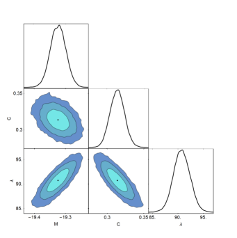
Figure 1: The posterior distributions at 1$\sigma$, 2$\sigma$ and 3$\sigma$ for the jerk model using OHD+Pantheon+ datasets.

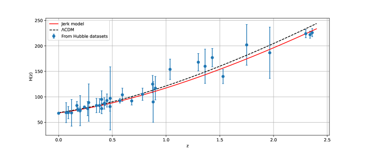
Figure 2: A good fit to the 31 points of the OHD datasets is displayed in the plot of $H(z)$ versus the redshift $z$ for our jerk model, which is shown in red, and $\Lambda$CDM, which is shown in black dashed lines.

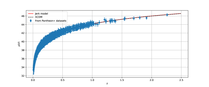
Figure 3: A good fit to the 1701 points of the Pantheon+ datasets is displayed in the plot of $\mu(z)$ versus the redshift $z$ for our jerk model, which is shown in red, and $\Lambda$CDM, which is shown in black dashed lines.

Datasets	OHD + Pantheon+
Model	$\Lambda$CDM	Jerk model
$\Omega_{m}$	$0.282\pm 0.0118$	-
$h$	$0.71\pm 0.0082$	-
$C$	-	$0.3133\pm 0.0095$
$\lambda$	-	$90.74\pm 1.632$
$M$	$-19.3235\pm 0.02317$	$-19.324\pm 0.0238$
$\chi^{2}_{min}$	$1564.111$	$1564.13$

Table 1: Summary of the mean$\pm 1\sigma$ of the cosmological parameters for the $\Lambda$CDM and jerk models, using the OHD + Pantheon+ datasets.

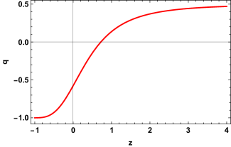
Figure 4: The graphical behavior of deceleration parameter in terms of $z$ i.e. Eq. (26) with the constraint values from OHD + Pantheon+ datasets.

III.2 Energy conditions

The energy conditions (ECs) are a set of alternative conditions that are used to put additional constraints on the validity of the constructed cosmological model and have many applications in theoretical cosmology. For example these conditions play an important role in GR as they help to prove theorems about the presence of the singularity of space-time and black holes [56]. In the context of this work, ECs are exploited in order to predict the acceleration phase of the Universe. Like these conditions can be obtained from the famous Raychaudhury equations, which forms are [57, 58, 59]

$$\frac{d\theta}{d\tau}=-\frac{1}{3}\theta^{2}-\sigma_{\mu\nu}\sigma^{\mu\nu}+\omega_{\mu\nu}\omega^{\mu\nu}-R_{\mu\nu}u^{\mu}u^{\nu}\,,$$ (34)

$$\frac{d\theta}{d\tau}=-\frac{1}{2}\theta^{2}-\sigma_{\mu\nu}\sigma^{\mu\nu}+\omega_{\mu\nu}\omega^{\mu\nu}-R_{\mu\nu}n^{\mu}n^{\nu}\,,$$ (35)

where $n^{\mu}$, $\theta$, $\omega_{\mu\nu}$ and $\sigma^{\mu\nu}$ are the null vector, the expansion factor, the rotation and the shear associated with the vector field $u^{\mu}$, respectively. In Weyl geometry with the existence of non-metricity scalar $Q$, the Raychaudhury equations take various forms, for more details see [60]. Next, the above equations (34) and (35) fulfill the conditions

$$R_{\mu\nu}u^{\mu}u^{\nu} \geq 0\,,$$ (36)

$$R_{\mu\nu}n^{\mu}n^{\nu} \geq 0\,.$$ (37)

Thus, if we examine the perfect fluid distribution of cosmological matter, the ECs for $f(Q)$ gravity are given as follows [37],

• Weak energy conditions (WEC) if $\rho_{eff}\geq 0$, $\rho_{eff}+p_{eff}\geq 0$.

• Null energy condition (NEC) if $\rho_{eff}+3p_{eff}\geq 0$.

• Dominant energy conditions (DEC) if $\rho_{eff}\geq 0$, $|p_{eff}|\leq\rho$.

• Strong energy conditions (SEC) if $\rho_{eff}+3p_{eff}\geq 0$.

By taking Eqs. (21) and (22) in the WEC, NEC, and DEC constraints, we can prove that

• Weak energy conditions (WEC) if $\rho\geq 0$, $\rho+p\geq 0$.

• Null energy condition (NEC) if $\rho+p\geq 0$.

• Dominant energy conditions (DEC) if $\rho\geq 0$, $|p|\leq\rho$.

These results are in concordance with those of Capozziello et al. [61]. In the case of the SEC condition, we find

$$\rho+3\,p-6\,\dot{f}_{Q}\,H+f\geq 0\,.$$ (38)

Now, using the above ECs, we can check the validity of our cosmological models in the following sections.

IV Cosmological $f\left(Q\right)$ models

In this section, we will discuss the proposed cosmological models and some of their physical properties such as the energy density, pressure and equation of state (EoS) parameter using the general solution of the jerk model parameter. In addition, we will verify our cosmological models with the help of the ECs described in the previous section. Here, we will propose two models of $f(Q)$ gravity. In the first model, we will assume a linear form of $f(Q)$. Then, in the second model we will take a non-linear functional form of $f(Q)$ gravity.

IV.1 Linear model $f\left(Q\right)=\alpha Q+\beta$

In this subsection, we presume the following simplest linear form of the $f(Q)$ function i.e.

$$f\left(Q\right)=\alpha Q+\beta$$ (39)

where $\alpha$ and $\beta$ are free parameters. The motivation behind this linear form is the cosmological constant, despite the problems it faces, it is considered to be the most successful model among the alternatives offered in cosmology. The results of this model have been discussed in several contexts [62, 63, 42, 43].

Using Eqs. (19) and (25), we get the energy density of the Universe in the form

$$\rho=\frac{3\beta\left(e^{2\lambda t}-1\right)^{2}-8\alpha\lambda^{2}\left(e^{2\lambda t}+1\right)^{2}}{6\left(e^{2\lambda t}-1\right)^{2}}.$$ (40)

Again, using Eqs. (20) and (25) we get the isotropic pressure of the Universe as

$$p=\frac{1}{6}\left(8\alpha\lambda^{2}-3\beta\right).$$ (41)

Thus, the EoS parameter ($p=\omega\rho$) for our model is

$$\omega=-\frac{\left(e^{2\lambda t}-1\right)^{2}\left(3\beta-8\alpha\lambda^{2}\right)}{3\beta\left(e^{2\lambda t}-1\right)^{2}-8\alpha\lambda^{2}\left(e^{2\lambda t}+1\right)^{2}}.$$ (42)

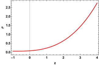
Figure 5: The graphical behavior of energy density in terms of $z$ with $\alpha=-0.5$ and $\beta=2$ for the specific case of $f\left(Q\right)=\alpha Q+\beta$.

From Fig. 5, we can observe that as the Universe expands, its energy density stays positive and decreasing function of cosmic time (or increasing function of redshift). Also, they tend to zero in the future. Moreover, the plot for EoS parameter in Fig. 6 shows quintessence-like behavior in the present, converges to the $\Lambda$CDM model in the future and to the dust matter in the past. Also, the present value of the EoS parameter corresponding to the OHD+Pantheon+ is $\omega_{0}=-0.7161$. Now, using Eqs. (40) and (41) in the above ECs, we have plotted the behavior of NEC, DEC, and SEC in terms of the cosmological redshift in Fig. 7. From this figure, it can be clearly seen that all the ECs are satisfied while the SEC is violated. This violation of the SEC is the evidence of the validity of the proposed cosmological model, and thus predicts the accelerating phase of the Universe.

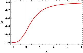
Figure 6: The graphical behavior of EoS parameter in terms of $z$ with $\alpha=-0.5$ and $\beta=2$ for the specific case of $f\left(Q\right)=\alpha Q+\beta$.

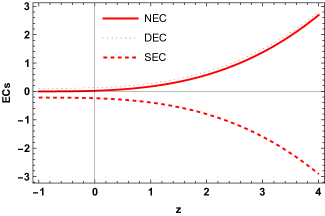
Figure 7: The graphical behavior of ECs in terms of $z$ with $\alpha=-0.5$ and $\beta=2$ for the specific case of $f\left(Q\right)=\alpha Q+\beta$.

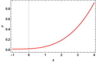
Figure 8: The graphical behavior of energy density in terms of $z$ with $m=-5$ and $n=1.08$ for the specific case of $f\left(Q\right)=Q+mQ^{n}$.

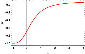
Figure 9: The graphical behavior of EoS parameter in terms of $z$ with $m=-5$ and $n=1.08$ for the specific case of $f\left(Q\right)=Q+mQ^{n}$.

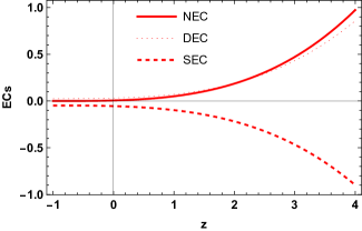
Figure 10: The graphical behavior of ECs in terms of $z$ with $m=-5$ and $n=1.08$ for the specific case of $f\left(Q\right)=Q+mQ^{n}$.

IV.2 Non-linear model $f\left(Q\right)=Q+mQ^{n}$

Here, for the second model, we discuss the non-linear functional form of $f(Q)$,

$$f\left(Q\right)=Q+mQ^{n}$$ (43)

where $m$ and $n$ are free parameters. Also, this specific form has been considered in many cosmological contexts [41, 38, 63].

Thus, for this specific choice, we get the energy density, the isotropic pressure and the EoS parameter as

$$\rho=\frac{2^{3n-1}3^{-n-1}\left(-3m(2n-1)\left(e^{2\lambda t}-1\right)^{2}\left(\frac{9}{4}H^{2}\right)^{n}-\lambda^{2}3^{n}8^{1-n}\left(e^{2\lambda t}+1\right)^{2}\right)}{\left(e^{2\lambda t}-1\right)^{2}},$$ (44)

$$p=\frac{3^{-n-1}\left(3m8^{n}(2n-1)\left((2-4n)e^{2\lambda t}+e^{4\lambda t}+1\right)\left(\frac{9}{4}H^{2}\right)^{n}+8\lambda^{2}3^{n}\left(e^{2\lambda t}+1\right)^{2}\right)}{2\left(e^{2\lambda t}+1\right)^{2}},$$ (45)

and

$$\omega=-\frac{\left(e^{2\lambda t}-1\right)^{2}\left(3m8^{n}(2n-1)\left((2-4n)e^{2\lambda t}+e^{4\lambda t}+1\right)\left(\frac{9}{4}H^{2}\right)^{n}+8\lambda^{2}3^{n}\left(e^{2\lambda t}+1\right)^{2}\right)}{\left(e^{2\lambda t}+1\right)^{2}\left(3m8^{n}(2n-1)\left(e^{2\lambda t}-1\right)^{2}\left(\frac{9}{4}H^{2}\right)^{n}+8\lambda^{2}3^{n}\left(e^{2\lambda t}+1\right)^{2}\right)},$$ (46)

respectively.

From Fig. 8, it is clear that the energy density of the Universe is an increasing function of cosmological redshift and remains positive as the Universe expands. In addition, it tends to zero in the future. Further, the plot for EoS parameter in Fig. 9 shows quintessence-like behavior in the present and converges to the $\Lambda$CDM model in the future and to the dust matter in the past. Further, the present value of the EoS parameter corresponding to the OHD+Pantheon+ is $\omega_{0}=-0.7009$. For this case, using Eqs. (44) and (45) in the above ECs, we have plotted the behavior of NEC, DEC, and SEC in terms of cosmological redshift in Fig. 10. From this figure, it is clear that all the ECs are satisfied but SEC is violated. This violation of the SEC is the evidence of the validity of the proposed cosmological model, and thus predicts the accelerating phase of the Universe.

V Discussions and conclusions

The standard model of cosmology ($\Lambda$CDM) is most widely accepted today as it has been able to explain a large number of observed phenomena: the expansion of the Universe, the existence of the cosmic microwave background and the big bang nucleosynthesis. However, as we have pointed out in the introduction, $\Lambda$CDM could not explain dark energy (DE) and other issues [64, 65]. These puzzles prompted many authors to search for suitable alternatives, and some scientists went so far as to suggest a modification of general relativity, the theoretical basis of the $\Lambda$CDM model.

In this paper, we have discussed one of these recently proposed theories which has attracted the attention of many researchers i.e. $f(Q)$ gravity where the non-metricity $Q$ is the basis of gravitational interactions with zero curvature and torsion. We have studied a homogeneous and isotropic FLRW space-time in the framework of this modified theory and the help of the jerk parameter. The jerk parameter can be employed in a number of scenarios. Chakrabarti et al. [50] proposed a reconstruction of extended teleparallel $f(T)$ gravity using this parameter. In this scenario, we used the jerk parameter to study the late-time expansion of the Universe in $f(Q)$ gravity. So, we have briefly described the mathematical formalism of $f(Q)$ gravity, then we have derived the field equations in the FLRW space-time for the content of the Universe in the form of a perfect fluid. Moreover, we have used $31$ data points of OHD and $1701$ data points of Pantheon+ to constrain the model parameters. The current Hubble rate and the deceleration parameter derived from the best fit of Markov Chain Monte Carlo (MCMC) are in agreement with those of the Planck data [12]. Moreover, we combined OHD + Pantheon+ datasets with recently published Pantheon+ datasets to get the model parameters that fit the data the best. The results of the best fit is $\lambda=90.74\pm 1.632$ and $C=0.3133\pm 0.0095$. In the same context, Mukherjee et al. [66] constrained a variables jerk parameters by means of MCMC. Furthermore, Ayuso et al. [67] employed the MCMC approach to constrain the general power model of $f(Q)$ gravity and determine the best-fit of cosmological parameter.

Next, we have considered two functional forms of $f(Q)$ gravity, specifically, a linear and a non-linear form. We have analyzed the behavior of different cosmological parameters such as energy density, pressure and EoS parameter for both models. we have also checked all energy conditions in order to ensure the validity of our proposed cosmological models. For both models, Figs. 5 and 8, we have found that the energy density of the Universe is a decreasing function of cosmic time (or increasing function of redshift) and remains positive as the Universe expands. Furthermore, from Figs. 6 and 9, we have observed that the EoS parameter behaves like a quintessence dark energy model in the vicinity of our present time, while in the future and in the past it behaves as the $\Lambda$CDM model and the dust matter, respectively for both models. Finally, from the energy conditions as shown in Figs. 7 and 10 we can conclude that all the energy conditions are satisfied for both models while SEC is violated. The results above demonstrate that our proposed cosmological models are in strong agreement with today’s observations.

Data availability There are no new data associated with this article

Declaration of competing interest The authors declare that they have no known competing financial interests or personal relationships that could have appeared to influence the work reported in this paper.

- [1] A.G. Riess et al., Astron. J. 116, 1009 (1998).
- [2] S. Perlmutter et al., Astrophys. J. 517, 565 (1999).
- [3] R.R. Caldwell, M. Doran, Phys. Rev. D 69, 103517 (2004).
- [4] Z.Y. Huang et al., JCAP 0605, 013 (2006).
- [5] T. Koivisto, D.F. Mota, Phys. Rev. D 73, 083502 (2006).
- [6] S.F. Daniel, Phys. Rev. D 77, 103513 (2008).
- [7] D.J. Eisenstein et al., Astrophys. J. 633, 560 (2005).
- [8] W.J. Percival at el., Mon. Not. R. Astron. Soc. 401, 2148 (2010).
- [9] C.L. Bennett et al., Astrophys. J. Suppl. 148, 119-134 (2003).
- [10] D.N. Spergel et al., [WMAP Collaboration], Astrophys. J. Suppl. 148, 175 (2003).
- [11] G. Hinshaw et al., Astrophys. J. Suppl. 208, 19 (2013).
- [12] N. Aghanim et al., Astron. Astrophys. 641, A6 (2020).
- [13] S.Weinberg, Rev. Mod. Phys. 61, 1 (1989).
- [14] B. Ratra and P.J.E. Peebles, Phys. Rev. D 37, 3406 (1998).
- [15] M. Sami and A. Toporensky, Mod. Phys. Lett. A 19, 1509 (2004).
- [16] C. Armendariz-Picon et al., Phys. Rev. Lett. 85, 4438 (2000).
- [17] J. Khoury and A. Weltman, Phys. Rev. Lett. 93, 171104 (2004).
- [18] T. Padmanabhan, Phys. Rev. D 66, 021301 (2002).
- [19] M. C. Bento et al., Phys. Rev. D 66, 043507 (2002).
- [20] R. Zarrouki and M. Bennai, Phys. Rev. D 82, 123506 (2010).
- [21] M. Bouhmadi-López, A. Errahmani, P. MartÃn-Moruno, T. Ouali, Y. Tavakoli, Internat. J. Modern Phys. D 24 (10), 1550078 (2015).
- [22] J. Morais, M. Bouhmadi-López, K. Sravan Kumar, J. Marto, Y. Tavakoli, Phys. Dark Univ. 15, 7 (2017).
- [23] M. Bouhmadi-López, D. Brizuela, I. Garay, J. Cosmol. Astropart. Phys. 1809 (09), 031 (2018).
- [24] A. Bouali, I. Albarran, M. Bouhmadi-López, T. Ouali, Phys. Dark Univ. 26, 100391 (2019).
- [25] A. Bouali, I. Albarran, M. Bouhmadi-López, A. Errahmani, T. Ouali, Phys. Dark Univ. 34, 100907(2021).
- [26] S. Capozziello et al., Phys. Lett. B 632, 597 (2006).
- [27] R.D. Blandford et al., arXiv preprint arXiv:astro-ph/0408279 (2004).
- [28] T. Chiba and T. Nakamura, Prog. Theor. Phys. 100, 1077 (1998).
- [29] V. Sahin, arXiv preprint arXiv:astro-ph/0211084 (2002).
- [30] M. Visser, Class. Quantum Gravity 21, 2603 (2004).
- [31] M. Visser, Gen. Relativ. Gravit. 37, 1541 (2005).
- [32] U. Alam et al., Mon. Not. Roy. Astron. Soc. 344, 1057–1074 (2003).
- [33] R.D. Rapetti et al., Mon. Not. Roy. Astron. Soc. 375, 1510 (2007).
- [34] M. Zubair and L. R. Durrani, Eur. Phys. J. Plus 135, 8 (2020).
- [35] J. Lu, L. Xu and M. Liu, Phys. Lett. B 699, 8 (2011).
- [36] Y. Xu et al., Eur. Phys. J. C 79, 8 (2019).
- [37] S. Mandal et al., Phys. Rev. D 102, 024057 (2020).
- [38] S. Mandal et al., Phys. Rev. D 102, 124029 (2020).
- [39] T. Harko et al., Phys. Rev. D 98, 084043 (2018).
- [40] N. Dimakis et al., Class. Quantum Grav. 38, 225003 (2021).
- [41] S. H. Shekh, Phys. Dark Universe 33, 100850 (2021).
- [42] M. Koussour et al., J. High Energy Astrophys 35, 43-51 (2022).
- [43] M. Koussour et al., Phys. Dark Universe 36, 101051 (2022).
- [44] J. B. Jimenez et al., Phys. Rev. D 98, 044048 (2018).
- [45] J. B. Jimenez et al., Phys. Rev. D 101, 103507 (2020).
- [46] J. V. Cunha and J. A. S. D. Lima, Mon. Notices Royal Astron. Soc. 390, 1 (2008).
- [47] E. Mortsell and C. Clarkson, J. Cosm. Astropar. Phys. 2009, 01 (2009).
- [48] S. K. J. Pacif et al., Int. J. Geom. Meth. Mod. Phys. 14, 7 (2017).
- [49] R. Lazkoz et al., Phys. Rev. D 100, 104027 (2019).
- [50] Chakrabarti et al., Eur. Phys. J. C 79, 454 (2019).
- [51] L. E. Padilla et al., Universe 97 (2021) 213. [arXiv:1903.11127]
- [52] G. S. Sharov V. O. Vasiliev, Appl. Math. Model 6 (2018) 1. [arXiv:1807.07323]
- [53] S. Joan , Phys. Rev. D . 71 (2005) 255-262. [arXiv:1209.0210]
- [54] J. E. Bautista et al., Astron. Astrophys. 603 (2017) A12. [arXiv:1702.00176]
- [55] D. Brout et al., Astrophys . J. 938 (2022) 110. [arXiv:2202.04077v2]
- [56] R. M. Wald, Chicago, IL: University of Chicago Press, (1984).
- [57] A. Raychaudhuri, Phys. Rev. D 98, 1123 (1955).
- [58] S. Nojiri and S. D. Odintsov, Int. J. Geom. Methods Mod. Phys. 04, 115 (2007).
- [59] J. Ehlers, Int. J. Mod. Phys. D 15, 1573 (2006).
- [60] S. Arora, et al., Phys. Dark Universe 31, 100790 (2021).
- [61] S. Capozziello, S. Nojiri, and S. D. Odintsov, Phys. Lett. B 781, 99 (2018).
- [62] R. Solanki et al., arXiv preprint arXiv:2201.06521 (2022).
- [63] Sokoliuk et al., arXiv preprint arXiv:2201.00743 (2022).
- [64] K. El Bourakadi et al., Eur. Phys. J. Plus 136, 8 (2021).
- [65] K. El Bourakadi et al., Eur. Phys. J. C 81, 12 (2021).
- [66] A. Mukherjee and N. Banerjee., Phys. Rev. D 93, 043002 (2016).
- [67] I. Ayuso et al., Phys. Rev. D 103, 6 (2021).