Towards Better Generalization with Flexible Representation
of Multi-Module Graph Neural Networks

Abstract

Graph neural networks (GNNs) have become compelling models designed to perform learning and inference on graph-structured data. However, little work has been done to understand the fundamental limitations of GNNs for scaling to larger graphs and generalizing to out-of-distribution (OOD) inputs. In this paper, we use a random graph generator to systematically investigate how the graph size and structural properties affect the predictive performance of GNNs. We present specific evidence that the average node degree is a key feature in determining whether GNNs can generalize to unseen graphs, and that the use of multiple node update functions can improve the generalization performance of GNNs when dealing with graphs of multimodal degree distributions. Accordingly, we propose a multi-module GNN framework that allows the network to adapt flexibly to new graphs by generalizing a single canonical nonlinear transformation over aggregated inputs. Our results show that the multi-module GNNs improve the OOD generalization on a variety of inference tasks in the direction of diverse structural features.

1 Introduction

Graph neural networks (GNNs) have recently been established as an effective machine learning models for representation learning on graph-structured data (Scarselli et al., 2008; Hamilton et al., 2017b; Bronstein et al., 2017; Battaglia et al., 2018). Graph is a powerful mathematical abstraction that can represent the structure of many complex data, and learning on graphs has been widely explored in many scientific domains (Duvenaud et al., 2015; Gilmer et al., 2017; Sanchez-Gonzalez et al., 2018; 2020; Gainza et al., 2020).

Despite the growing empirical success of GNNs in various fields, the necessity of a deeper understanding of this model framework has arisen due to the inconsistent model efficiency across different tasks and experimental settings. Building large-scale graph benchmarks (Dwivedi et al., 2020; Hu et al., 2020) is one recent attempt to address this challenge, and there have also been significant theoretical studies on the expressivity of GNNs focused on the isomorphism task (Xu et al., 2019; Morris et al., 2019; Garg et al., 2020; Sato, 2020; Morris et al., 2021). However, little work has been conducted on understanding the fundamental limitations of GNNs for adapting to distribution shifts on graphs, where systematic differences between training and test data can significantly degrade model performance.

Recent approaches to OOD generalization (Ovadia et al., 2019; Arjovsky et al., 2019; Ahuja et al., 2021; Lu et al., 2021) concentrate primarily on images or structural equation models. However, the nature of the graph domain is fundamentally different from these works in that the inputs are not simple image features or variables, but full of complex irregularities and connectivity in topology. We hypothesize that the difference in underlying graph properties of training and testing datasets (i.e. structural distribution shift) presents a fundamental challenge to the extrapolation beyond the range of input distribution. We are particularly interested in the conditions under which we can expect GNNs to (not) perform well in predicting targets for unseen graphs. To study this question, we use a random graph generator that allows us to systematically investigate how the graph size and structural properties affect the predictive performance of GNNs.

We argue that, among the many graph properties, the average node degree within each mode of the degree distribution is a key factor that determine whether GNNs can generalize to unseen graphs. Then, we propose and explore methods for using multiple node update functions as a way to generalize a single canonical nonlinear transformation over aggregated inputs. This approach enhances the flexibility of the network to handle shifts in graph properties, resulting in better control over structural distribution shifts. We evaluate the performance of the multi-module GNN framework on the task of approximating marginal inference for general graphs (Pearl, 1988), solving graph theory multi-task problems (Corso et al., 2020), conducting CLRS algorithmic reasoning tasks (Veličković et al., 2022), and benchmarking against OOD scenarios for real-world graphs (Gui et al., 2022). Our key contributions are as follows:

1. In Section 3.1, we present a diverse and densely populated random graph benchmark that enables the identification of visually recognizable and spatially characterized generalization patterns of GNNs. The random graphs offered in this study can be utilized as a useful testbed for graph OOD benchmark, as they allow for the integration of task-specific node/edge/graph-level input features and target outputs.

2. In Section 5.1, we identify a strong generalization pattern in OOD scenarios that is strongly correlated with the average node degree of in-distribution (ID) training graphs. This pattern remains consistent across various graph sizes, tasks, and baseline GNN models.

3. In Section 5.2, we demonstrate that having multiple modes in the degree distribution can impede OOD generalization, as it alters the distribution of incoming messages. Therefore, when evaluating generalization on unknown graphs, we suggest that it is important to consider the average node degree for each mode of the degree distribution separately instead of evaluating the distribution as a whole.

4. In Section 4, we propose a multi-module GNN framework designed to leverage multiple update modules to process complex messages aggregated from nodes in far modes of the degree distribution, leading to improved OOD generalization for several inference tasks (Section 5.3).

2 Preliminaries

The defining feature of GNNs is the form of neural message passing where vector messages are exchanged between nodes and updated on arbitrary graph structure using neural networks (Gilmer et al., 2017). The message passing operation that underlies variants of GNNs follows a common strategy: at each iteration, every node computes incoming MESSAGEs ($\mathcal{M}$) from its local neighborhood, AGGREGATEs ($\bigoplus$) them, and UPDATEs ($\mathcal{U}$) its node state $\bh_{i}$ by

$$\bh_{i}^{(t+1)}=\mathcal{U}\left(\bh_{i}^{(t)},\bigoplus_{(j,i)\in\mathcal{E}}\mathcal{M}\left(\bh_{i}^{(t)},\bh_{j}^{(t)},\bz_{i,j}\right)\right)$$ (1)

where $\bz_{i,j}$ represents the feature embedding vectors for input nodes $i,j$ in the node set $\mathcal{V}$ and for the edge $(j,i)$ in the edge set $\mathcal{E}$, and $\mathcal{M}$ and $\mathcal{U}$ are arbitrary differentiable functions (i.e., neural networks). The iterative scheme relies on reusing and sharing the three main mathematical operations (i.e., MESSAGE, AGGREGATE, and UPDATE) across computational graphs, where functional modules can operate on graphs of varied sizes and structures. Such a flexible design principle allows GNNs to be related to standard neural network layers (Battaglia et al., 2018).

As an illustrative example, multilayer perceptron (MLP) layers, where each node takes in the sum (AGGREGATE) of weighted inputs (MESSAGEs) from a previous layer and passes (UPDATEs) it through a fixed nonlinear activation function, are comparable to GNN layers (Figure 1a), although the all-to-all relations between MLP layers are different from the GNN relations defined by the edges. As conceptual extensions from scalar to vector-valued inputs, a shared UPDATE function in GNNs can be viewed as the same elementary building block as a canonical activation function such as ReLU in MLPs, in the sense that they all perform nonlinear transformations over aggregated inputs (Figure 1a). From this point of view, the proposed idea of using multiple update functions in GNNs is analogous to the use of multiple activations in MLPs (Figure 1b).

The motivation behind the use of multiple nonlinearities is to simulate the effect of diverse nonlinear cell properties in the brain (Douglas & Martin, 1991; Shepherd, 2004). Recent work has demonstrated that the task-dependent relative proportion of two distinct cell types allows sample-efficient learning and improves the generalization performance on orientation discrimination tasks (Bordelon & Pehlevan, 2022). The fact that an optimal mixture of two different cell types exists suggests that more than one nonlinear function •ype might be required for better generalization. The benefits for machine learning at this level of collective nonlinear input-output relationships remain unclear, and to the best of our knowledge, this is the first study to characterize the impact of multi-module nonlinear functions and their usefulness in the generalization of GNNs.

Figure 1: Overview of the proposed model structures. (a) GNN layer (left) and MLP layer (right) with a fixed nonlinear update/activation function (gray triangles). (b) The same layers with two different nonlinearities (green and orange triangles).

3 Experimental Setup

In this section, we present our approach for generating random graphs and analyzing their graph properties through visualization. Then we detail how these random graphs will be applied to specific graph benchmarks.

3.1 Random graph benchmark

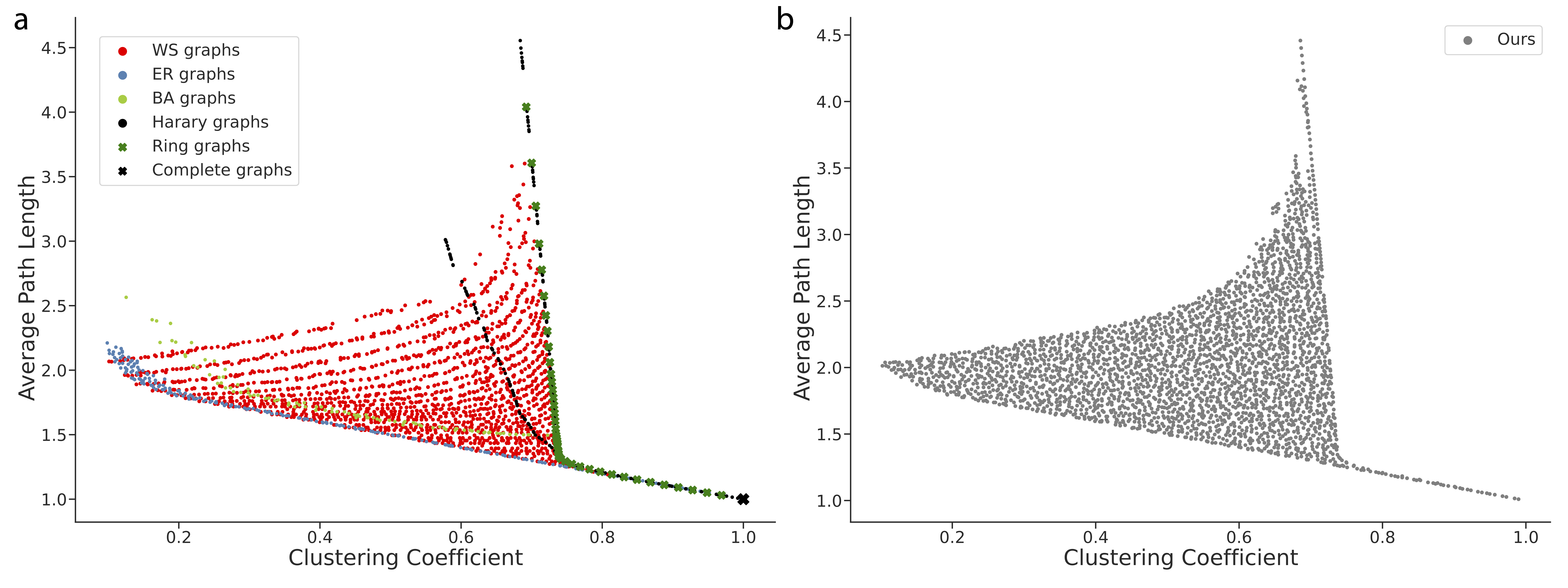
Figure A1: Coverage of random graphs. (a) Graphs sampled from four distinct random graph generators, along with ring and complete graphs having a size of $|\mathcal{V}|=100$. (b) Random graphs generated through our method, which covers a more extensive area of the graph space.

Random graph generator Our goal is to create a random graph generator that can produce a diverse set of graphs with a wide range of graph properties. Building on previous work (You et al., 2020), we have relaxed the constraint of the Watts-Strogatz model to allow for different node degrees before random rewiring. To generate a graph with $n$ nodes and an average node degree of $k$, we first set the number of edges to $e=\lfloor\frac{nk}{2}\rfloor$. Then, we construct a ring graph in which each node is connected to its $\lfloor\frac{e}{n}\rfloor$ subsequent neighbors. After that, we randomly select $e\;\mathrm{mod}\;n$ nodes and connect them to their nearest unconnected neighbors. Finally, we randomly rewire all edges with probability $p$. By repeating this process with different random seeds for each parameter setting, we have generated a total of 3,600,000 random graphs (more information is provided in Appendix A.1). This method, although it appears to be a single model, can generate a variety of graphs that encompass those produced by classic random graph generators like Erdős-Rényi (Erdos et al., 1960), Watts-Strogatz (Watts & Strogatz, 1998), Barabási-Albert (Albert & Barabási, 2002), and Harary (Harary, 1962) models, including ring and complete graphs (Figure A1).

Visualizing structural properties of random graphs We next compute six graph properties for all samples. These include the average shortest distance between nodes (average path length), the fraction of connected triangles in a graph (clustering coefficient), the average, maximum, minimum, and standard deviation of node degrees. Each graph is then characterized by six measures, and the value of these variables can be naturally mapped to a point (vector) in a six-dimensional (6D) space where each axis represents one of the variables (Figure 2a). If there are a large number of graphs and the points are close to one another, they can form a cluster with distinct components in this space (Figure 2a). To better understand the distribution of sampled graph properties, we use principal component analysis to reduce the 6D space to 2D and visualize them by presenting the recorded measures for each sampled graph as color-coded scatter plots (Figure 2b). The visualized results demonstrate the development of the structural properties of the sampled graphs in a low-dimensional space (Figure 2b). The progression in these patterns will be used as a means for evaluating the generalization capabilities of GNNs.

Data split for OOD tasks This set of large random graphs serves as a test bed for assessing the generalization performance of proposed models in OOD settings. Specifically, we choose five evenly spaced locations on a 2D scatter plot, as shown in Figure 2c. We then collect all samples within a circle of a half-unit radius centered on each position and consider only non-isomorphic graphs. The resulting set $\mathcal{G}_{i}$ of non-isomorphic graphs obtained from the $i$-th location composes a distinct set of training graphs (Figure 2c). The number of training samples in each group may differ slightly; thus, we ensure that the sample count is consistently 1,000 across the five groups $\mathcal{G}_{i=1:5}$ by providing different input features to the graphs. For the test graphs $\mathcal{G}_{\textrm{test}}$, we uniformly sub-sample $\sim$1,000 graphs from the entire sample space ($N$=3.6M) as in Figure 2c (more details in Appendix A.1). Since the training split occupies a small portion of the sample space compared to the test split, this data split is appropriate for studying OOD generalization in the presence of structure shift. In our experiments for the presented benchmark, we use graphs with small to medium sizes ranging from 16 to 100 nodes.

Figure 2: Random and real-world graph benchmarks. (a) Illustration of random graph space where each axis $p_{i}$ represents a graph measure. Inset: Three examples of 100-node graphs (stars) with different connectivity levels. (b) 2D scatter plots showing the distribution of each of the six graph properties across the entire dataset (N=3.6M graphs). (c) Left: The graphs (gray dots) in red circles constitute five distinct sets $\mathcal{G}_{i=1:5}$ of training graphs, Right: Uniformly sub-sampled test graphs (gray dots). (d) Seven distinct real-world graph benchmarks are displayed with different colors, and they are superimposed on each other. To avoid confusion arising from overlapping distributions, each dataset is independently re-visualized along the orthogonal direction in 2D space.

3.2 Specific tasks for input features and targets

Our random graph dataset can be used for various tasks in graph representation learning simply by assigning node and edge features with corresponding targets to the predefined graph structures. We first consider two specific tasks in this work: (1) an approximate marginal inference task that is intractable for general graphs and (2) a multi-task graph theory problem consisting of three node-level and three graph-level prediction tasks. Since these two tasks are defined on the previously created random graphs, we manually generate synthetic input features and target outputs for each task.

Marginal inference task Computing marginal probability distributions of task-relevant variables at each node of a graph is often computationally intractable, and thus relies on approximate methods (Pearl, 1988; Wainwright et al., 2003). We follow the setup of recent work improving message-passing algorithms by GNNs (Yoon et al., 2018; Satorras & Welling, 2021). Specifically, we evaluate the generalization performance in Markov random fields (Ising model) comprising binary variables $\bx\in\{+1,-1\}^{|\mathcal{V}|}$, each with an associated bias $b_{i}$ and coupling strength $J_{ij}$ via the following parameterization:

$$p(\bx;{\bm{\theta}})=\frac{1}{Z({\bm{\theta}})}\exp\left(\sum_{i\in\mathcal{V}}b_{i}x_{i}+\sum_{(i,j)\in\mathcal{E}}J_{ij}x_{i}x_{j}\right)$$ (2)

The collective model parameters ${\bm{\theta}}=\{b_{i}\}_{i\in\mathcal{V}}\cup\{J_{ij}\}_{(i,j)\in\mathcal{E}}$ determine the state of each variable node, given the state of other connected nodes. The number of nodes $|\mathcal{V}|$ and the connectivity structure $\mathcal{E}$ are determined by our random graph benchmark. The Ising model parameter ${\bm{\theta}}$ is sampled from a standard normal distribution $\mathcal{N}(0,1)$, where the sampled bias $\{b_{i}\}$ and coupling weight $\{J_{ij}\}$ are provided as input node and edge features of GNNs, respectively. For the sake of the targets, we calculate marginal probabilities $p(x_{i})$ for each node $i\in\mathcal{V}$ of small graphs ($|\mathcal{V}|=16$) using brute-force enumeration, whereas we run a Markov Chain Monte Carlo (MCMC) algorithm, the Gibbs sampler (Geman & Geman, 1984), on larger graphs ($|\mathcal{V}|=36,100$). We accept the approximate marginals as ground truth targets when the mean absolute error of the estimates from the Gibbs sampler with respect to the counterpart of the binary Hamiltonian Monte Carlo (Pakman & Paninski, 2013) falls below 0.02, suggesting that convergence is reached for the MCMC chains: $\left\langle\left|p_{\text{Gibbs}}(x_{i})-p_{\text{HMC}}(x_{i})\right|\right\rangle_{i\in\mathcal{V}}\leq 0.02$.

Graph theory multi-task We also investigate classical graph theory problems at both the node and graph levels. At the node level, we focus on predicting single-source shortest path lengths, eccentricity, and Laplacian features, while at the graph level, we aim to determine diameter, spectral radius, and whether the graph is connected. These tasks were initially addressed by Corso et al. (2020), but in this work, we evaluate them on 100-node random graphs that are more diverse in structure and larger in size than in previous studies. As input features, the graph is provided with two types of position indices for each node: a one-hot vector representing the source for the shortest path task and a random scalar uniformly sampled from the range of [0,1].

3.3 Real-world graph benchmark

In order to explore the practical implications of our proposed model framework beyond the random graph benchmark, we have also considered real graph benchmark datasets and visualized their graph properties in the 2D scatter plot (Figure 2d). Our aim is to gain a better understanding of how real-world graphs are distributed and assess whether they accurately represent the full range of graph properties. Interestingly, we discover that most of these datasets have limitations either by sparsely populating or occupying only a small portion of the graph space (Figure 2d). This supports the idea that our random graph benchmark is beneficial for studying structural shifts in distribution, rather than solely relying on real-world scenarios. Nevertheless, we intend to experiment with the proposed ideas using real-world datasets and then evaluate the outcomes by comparing them with our observations from studying the random graph benchmark. Ultimately, this will enable us to validate the practical utility of our approach.

CLRS algorithmic reasoning tasks The CLRS benchmark is a recent comprehensive dataset that includes 30 highly complex classical algorithmic reasoning tasks (Veličković et al., 2022). Although most algorithms in CLRS are based on smaller graphs generated from a single Erdős-Rényi model, we have opted to evaluate our proposed methods using CLRS because it is a leading benchmark for investigating OOD generalization in graph domains. The summary of dataset configuration is provided in Table A4.

GOOD: Graph OOD benchmark GOOD (Gui et al., 2022) is the latest real-world graph OOD benchmark designed to be challenging by making distinct shifts in input or target distribution (i.e. covariate and concept shifts). It provides 6 graph-level and 5 node-level prediction tasks, covering a range of datasets from molecular graphs and citation networks to colored MNIST datasets. Our focus is on graph prediction tasks exclusively (more details in Table A4), as the node-level tasks are all based on a single graph (i.e., transductive setting), which falls outside the scope of our study that aims to explore generalization to unseen graphs across multiple graphs.

4 Multi-module GNNs

We next present various strategies for building multi-module GNNs. The GNN architecture that we examine utilizes an encode-process-decode framework (Battaglia et al., 2018) as depicted in Figure 3a, and the baseline processor is based on the message-passing neural network (MPNN; Gilmer et al., 2017), as outlined in Equation 1. Additionally, we incorporate the graph attention mechanism (GAT; Veličković et al., 2018) when appropriate to improve generalization performance. The update function in the processor is a crucial component of the proposed methods and plays a vital role in the performance of GNNs. Thus, we outline three different strategies for leveraging two update modules within our framework.

4.1 Multi-module sigmoid gating

The first approach is to use a sigmoid gating mechanism (Figure 3b, left), where the values of the learned gates determine the utilization of multiple update modules. Specifically, the next hidden state $\bh_{i}^{(t+1)}$ is computed by taking a linear combination of two intermediate node states $\bh_{i,1}^{(t)}$ and $\bh_{i,2}^{(t)}$ as follows:

$$\bh_{i}^{(t+1)} =\;\alpha_{i}^{(t)}\bh_{i,1}^{(t)}+(1-\alpha_{i}^{(t)})\bh_{i,2}^{(t)}$$ (3)

where the two intermediate representations $\bh_{i,1}^{(t)}$ and $\bh_{i,2}^{(t)}$ are the outputs of Equation 1 using distinct update functions $\mathcal{U}_{1}$ and $\mathcal{U}_{2}$, respectively. The value of the gating variable $\alpha_{i}^{(t)}$ is obtained from another processor but replacing $\mathcal{U}$ with a gating function $\phi_{g}$, which is a neural network with a sigmoid activation for the scalar output.

4.2 Multi-module binary gating

The second approach for updating the node states in our model involves using a binary gating mechanism (Figure 3b, middle), where a binary decision is made between two different update modules using the Gumbel reparameterization trick (Jang et al., 2017; Maddison et al., 2017). Unlike the sigmoid gating method, this approach allows to only applies one specific update module to each node. To accomplish this, we set $\alpha_{i}^{(t)}$ as a random variable with a Bernoulli distribution, parameterized by $\pi_{i}^{(t)}\in[0,1]$, such that $\alpha_{i}^{(t)}\sim\textrm{Ber}(\pi_{i}^{(t)})$. However, this parameterization poses a challenge in terms of differentiability, as the gradient does not flow through $\alpha_{i}^{(t)}$ in a typical Bernoulli sampling. To overcome this issue, we apply the Gumbel reparameterization trick as follows:

$$\alpha_{i}^{(t)}=\sigma\left(\frac{\log(\pi_{i}^{(t)}/(1-\pi_{i}^{(t)}))+(g_{i,1}^{(t)}-g_{i,2}^{(t)})}{\tau}\right)$$ (4)

where $g_{i,1}^{(t)},g_{i,2}^{(t)}\sim\texttt{\small Gumbel}(0,1)$, $\pi_{i}^{(t)}$ is the output of $\phi_{g}$, and $\alpha_{i}^{(t)}=1$ with probability $\pi_{i}^{(t)}$ as the temperature $\tau$ approaches 0. In this way, the next node state $\bh_{i}^{(t+1)}$ becomes one of two intermediate representations $\bh_{i,1}^{(t)}$ and $\bh_{i,2}^{(t)}$. The binary gating strategy can be considered as sitting in the middle of the spectrum among the three strategies we introduce. During the forward pass, binary gating employs discrete sampling similar to the approach described next in multi-module meta-learning, while during the backward pass, computations are carried out on a computational graph defined by multiple modules, akin to sigmoid gating.

Figure 3: Multi-module GNNs. (a) Illustration of an encode-process-decode framework with the emphasis on the processor as a message-passing neural network. Every node (black dot) computes incoming messages (black arrows), aggregate (vertical line) them, and updates (triangle) its node state. (b) Three different ways of leveraging two update modules (orange and blue triangles): sigmoid gating (left), binary gating (middle), and multi-module meta-learning (right). (c) The multi-module GNN meta-learns a set of update modules, and at meta-test time, the system only needs to determine which modules should be replaced to make the most accurate predictions based on the observed data.

4.3 Multi-module meta-learning

The last strategy is to learn a set of update modules that can be inserted in various combinations at different nodes within the processor (Figure 3b, right). This method is significantly different from the previous gating mechanism as the selection of the modules and the updating of their parameters take place at different phases through meta-learning (Schmidhuber, 1987; Thrun & Pratt, 2012). In particular, the goal is to distribute two update modules across all nodes of a graph and search over the set of possible structures to find the one that best generalizes in OOD settings. The idea behind this composition is to flexibly reuse and recombine a finite number of update modules to ultimately achieve combinatorial generalization (Tenenbaum et al., 2011; Andreas et al., 2016; Ellis et al., 2018; Alet et al., 2018).

To be specific, let $\Theta=({\bm{\theta}}_{1},{\bm{\theta}}_{2},{\bm{\theta}}_{\text{rest}})$ be the weights of update modules $\mathcal{U}_{1},\mathcal{U}_{2}$, and the rest of a multi-module GNN. During meta-training, an optimal assignment $\mathcal{A}$ of two modules is determined for each node in training graphs $\mathcal{G}_{i}^{\text{train}}$, given a fixed set of model parameters $\Theta$. We then update $\Theta$ using test graphs $\mathcal{G}_{i}^{\text{test}}$, while maintaining the previously determined module allocation $\mathcal{A}$ for each graph (Figure 3c). This is achieved by using the BounceGrad algorithm (Alet et al., 2018), which alternates between steps of simulated annealing for improving $\mathcal{A}$ and gradient descent for optimizing $\Theta$ to minimize the predictive loss $\mathcal{L}$:

$$\mathcal{L}(\Theta)=\sum_{i}\ell\left(\mathcal{G}_{i}^{\text{test}},\,\mathop{\arg\min}_{\mathcal{A}_{i}\in\mathbb{A}}\ell\left(\mathcal{G}_{i}^{\text{train}},\mathcal{A}_{i},\Theta\right),\Theta\right)$$ (5)

In meta-testing phase, we assume the presence of a small number of final training graphs, $\mathcal{G}^{\text{train}}_{\text{meta-test}}$. These are not OOD samples, but rather a limited number of ID graphs. In general, meta-learning algorithms do not share the same task between the meta-training and meta-testing datasets. However, in our approach, we define a task as finding an optimal module assignment for each individual graph in the meta-training phase, while a new task in the meta-testing phase is defined as finding a single module structure that is applicable to all graphs in $\mathcal{G}^{\text{train}}_{\text{meta-test}}$. The objective is to search for a final optimal assignment of update modules over all possible arrangements $\mathbb{A}$ given $\mathcal{G}^{\text{train}}_{\text{meta-test}}$ with fixed $\Theta$:

$$\mathcal{A}^{*}=\mathop{\arg\min}_{\mathcal{A}\in\mathbb{A}}\ell\left(\mathcal{G}^{\text{train}}_{\text{meta-test}},\mathcal{A},\Theta\right)$$ (6)

The generalization performance is then evaluated on OOD test split, using the optimal structure $\mathcal{A}^{*}$. It is important to note that, in contrast to the gating mechanism, the type of update function selected for each node is no longer influenced by the test dataset at the final evaluation.

5 Results

We now presents a series of controlled experiments on the random graph benchmark to evaluate the generalization capability of GNNs. Our main objective is to pinpoint key factors that can consistently determine the ability of GNNs to generalize well on OOD inference tasks. We then proceed to examine how the incorporation of multiple update modules within a general GNN framework can enhance their OOD generalization across these tasks.

5.1 Degree matters in OOD generalization

To gain insight into the predictive performance of GNNs, we first consider the marginal inference task. In this task, the models are trained on each group $\mathcal{G}_{i}$ with a size of $|\mathcal{V}|=100$, and are tested on $\mathcal{G}_{\textrm{test}}$ of the same size but with different structures. We use the Kullback-Leibler (KL) divergence as a validation metric and present the results in a heat map (Figure 4a). To do this, we down-sample and aggregate the test graphs in Figure 2c into a coarse resolution of 900 (=30$\times$30) 2D spatial bins, where each bin records the average KL divergence of the graphs within it. For display purpose, we compute the average values in log scale and present them with contrasting colors, with blue indicating a lower KL divergence (or more accurate predicted marginals) and red indicating the opposite. If GNNs only learned representations of the training graphs, we would expect to see a small blue region around the training set $\mathcal{G}_{i}$. However, all experiments produce a non-trivial vertical band-like pattern translated by the location of $\mathcal{G}_{i}$ (Figure 4a). It is noteworthy that this vertical pattern aligns with the distribution of similar average node degrees in 2D scatter plot shown in Figure 2b.

Figure 4: Structural distribution shift and size generalization (a) Generalization performance on a 2D subspace as training graphs change from $\mathcal{G}_{1}$ to $\mathcal{G}_{5}$. Blue indicates a lower KL divergence (more accurate prediction), while red denotes a higher KL divergence (less accurate prediction). (b) Normalized node degree histograms generated from the training graphs (yellow) and the test graphs with the top 30% predictive performance (blue). (c) Same as Figure 4a except that the model is trained and evaluated on smaller graphs with $|\mathcal{V}|=16$. (d-e) Testing on larger graphs, $|\mathcal{V}|=36$ and $|\mathcal{V}|=100$, respectively. The inset in (e) depicts the magnified region of interest.

To further investigate the role of average node degree in the generalization pattern of GNNs, we generate a normalized histogram of the degrees of every node in the test graphs with the top $30\%$ predictive performance (Figure 4b, blue) and of all training graphs (Figure 4b, yellow). The histograms should have the same peak location if the band-like pattern results from the average degree of training graphs. We observe that the histogram from the testing graphs is unimodal, and the peak location closely coincides with the counterpart of the training graphs (Figure 4b), indicating that the average node degree is a critical feature in predicting GNNs’ generalization capabilities to unseen graphs. It is worth noting that this generalization pattern is not a feature only seen in the marginal inference task, but is consistently observed across other tasks and baseline GNN models (Figure A2). This suggests that the pattern is not influenced by the specific task and type of GNN architecture employed.

We next examine the size generalization problem by keeping the size of the training graphs small, with $|\mathcal{V}|=16$, and gradually increasing the size of the test graphs to $|\mathcal{V}|\in\{16,36,100\}$. To achieve this, we generate a new set of 3.6M random graphs with a size of $|\mathcal{V}|=16$, create four sets of training graphs $\mathcal{G}_{i=1:4}$, sub-sample $\mathcal{G}_{\text{test}}$, and perform the same marginal inference task as previously described. If the average degree were still a crucial factor, we would expect to see a band-like pattern that is not affected by the size of the training and testing graphs. Additionally, the corresponding histograms of node degrees should also appear superimposed. Indeed, we find that GNNs trained on $\mathcal{G}_{i}$ with a size of $|\mathcal{V}|=16$ produce a pattern like a vertical band aligned with the center of $\mathcal{G}_{i}$, and the normalized histogram from $\mathcal{G}_{i}$ provides excellent matches to the peak of the histogram obtained from $\mathcal{G}_{\text{test}}$ consistently across the same size (Figure 4c) and larger (Figure 4d-e) test graphs. This result suggests that the graph size may not be a fundamental limiting factor for the generalization in GNNs when the average node degree remains invariant across the training and testing distributions.

5.2 Multimode degree distribution as an impediment to OOD generalization

In the previous section, we observe that the degree distribution of graphs on which GNNs generalize well is characterized by a single mode, due to the relatively uniform degrees of the training graphs. However, it is still unclear if the average degree continues to be a significant factor in generalization when training on graphs with highly distinct node degrees. To address this, we create a new training split $\mathcal{G}_{\text{t}rain}$ by combining two existing sets of 100-node graphs, $\mathcal{G}_{2}$ and $\mathcal{G}_{4}$, resulting in a sample size ($N$=2000) twice larger than before.

In Figure 5a, the test performance of GNNs trained on $\mathcal{G}_{\text{t}rain}$ is compared to those trained on $\mathcal{G}_{2}$ and $\mathcal{G}_{4}$, respectively. The generalization pattern now becomes dual band-like, with a separation determined by the gap between $\mathcal{G}_{2}$ and $\mathcal{G}_{4}$ (Figure 5a, middle). This is also reflected in the bimodal appearance of the degree histogram (Figure 5b, middle). These results indicate that the average node degree is not the sole determining factor for generalization, but rather it plays a role in each mode of the degree distribution when evaluating OOD generalization for unknown graphs. Notably, the overall predictive performance for graphs within the pattern decreases significantly when trained simultaneously on $\mathcal{G}_{2}$ and $\mathcal{G}_{4}$ compared to when trained individually (Figure 5a-b). This finding suggests that even within a fixed set of graphs, the change in graph composition from a single-mode to multi-mode degree distribution hinders the OOD generalization of GNNs.

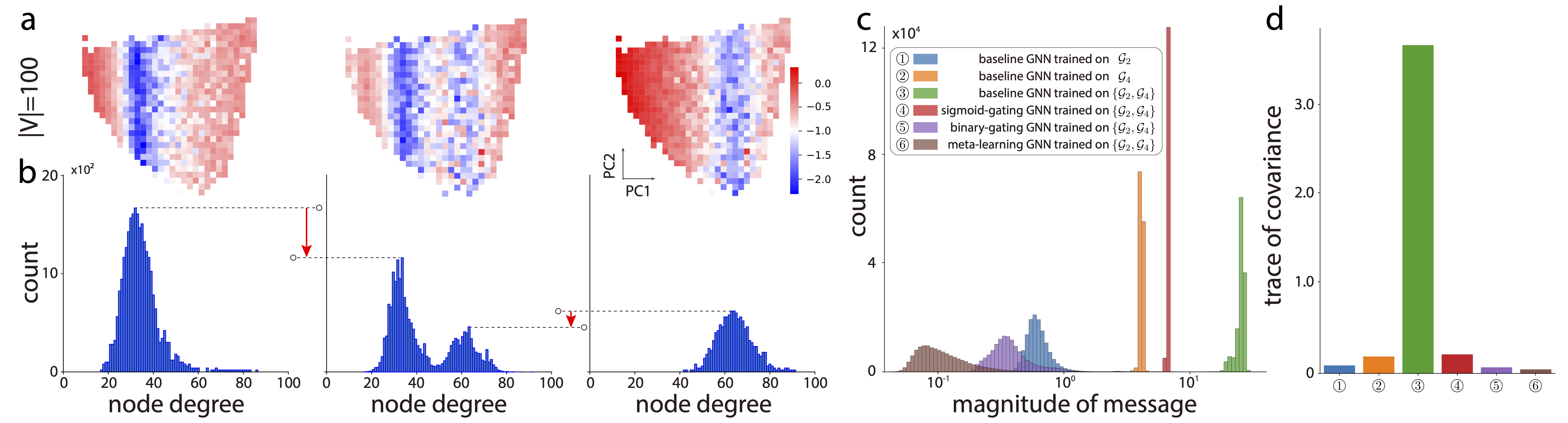
Figure 5: Effect of bimodal degree distribution on the predictive performance. (a) OOD performance of GNNs when trained on $\mathcal{G}_{2}$ (left), $\mathcal{G}_{2}\&\mathcal{G}_{4}$ (middle), and $\mathcal{G}_{4}$ (right). (b) Node degree histograms. The number of well-predicted graphs decreases substantially (red arrows) when jointly trained on $\mathcal{G}_{2}\&\mathcal{G}_{4}$. (c) The magnitude and (c) the total variance of message vectors gathered from both the baseline and multi-module GNNs.

We speculate that the degraded performance might be due to the change in the statistics of aggregated messages from nodes with multi-mode degree distributions. To test this hypothesis, an additional experiment is performed where the aggregated message is initially collected from each node in a graph from the GNN models trained on $\mathcal{G}_{2}$, $\mathcal{G}_{4}$, and $\mathcal{G}_{\text{t}rain}$, respectively. This procedure is then repeated for all test graphs to acquire a large message sample. We then compute (1) the magnitude and (2) the spread of messages by computing the trace of the covariance matrix of messages (Figure 5c-d). The results reveal that the magnitude of messages significantly increases, and the trace of covariance, which is the total variance of messages, becomes much larger when the baseline model is trained on $\mathcal{G}_{2}$ and $\mathcal{G}_{4}$ simultaneously compared to when it is trained separately (Figure 5c-d and Figure A3). The findings indicate that a switch from a unimodal to a multimodal degree distribution leads to a corresponding shift in the summary statistics of the message distribution, which may have created difficulties in the training of GNNs. This situation is similar to the one where several techniques for network initialization (Glorot & Bengio, 2010; He et al., 2015) or normalization (Ioffe & Szegedy, 2015; Ba et al., 2016) have been developed to maintain the mean or variance of activations during the training of deep neural networks.

5.3 Multi-module GNN framework for improving OOD generalization

Our multi-module training framework is proposed to address the issue and achieve improved generalization performance. The framework provides complementary update functions for processing those messages and exploring a diverse set of module combinations during training, which could potentially benefit from an ensemble effect in complex scenarios where the distribution of aggregated messages becomes more intricate. The message analysis applied to this new model framework shows that incorporating multiple update modules in a multimodal degree scenario reduces both the magnitude and variance of incoming messages. This reduction remains significant in some cases, even when compared to the single-module baseline trained on $\mathcal{G}_{2}$ or $\mathcal{G}_{4}$ (Figure 5c-d). The results from the previous section and the current analysis lead us to consider these training and test splits as a favorable OOD scenario, as it provides ample opportunity for improving OOD performance. Thus, we aim to address how multi-module GNNs are generalized to this OOD setting for the problems of marginal inference and graph theory multi-task, and show that the multi-module framework brings performance gains over the single-module baseline.

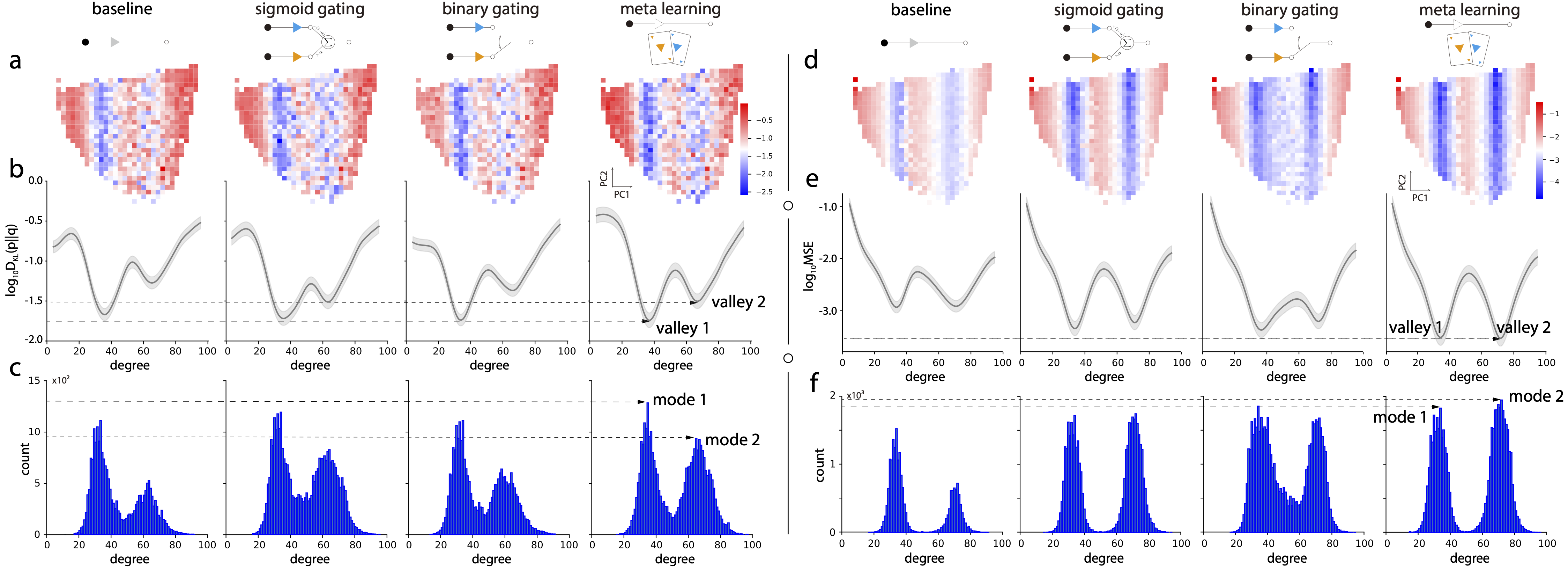
Figure 6: Performance of different multi-module GNN strategies on (a-c) marginal inference task and (d-f) graph theory multi-task. Each column is arranged in the following order: a single module baseline, and multi-module GNNs using sigmoid gating, binary gating, and meta-learning. (a,d) Test performance of GNNs when trained on $\mathcal{G}_{2}\&\mathcal{G}_{4}$. (b,e) Test KL-divergence loss in log scale (mean $\pm$ sd) (c,f) Node degree histogram from the test graphs with the top 40% predictive performance. For ease of comparison, the peak/bottom of each mode/valley in the rightmost column (best model) is highlighted by dashed lines.

Table 1: Test performance of single-module baseline and three different multi-module GNN strategies over 2 benchmark tasks.

Evaluation Metric
Method	Baseline	Sigmoid gating	Binary gating	Meta learning
Marginal Inference
Loss @ (valley 1, valley 2)	(-1.68, -1.28)	(-1.73, -1.52)	(-1.75, -1.38)	(-1.74, -1.51)
# of nodes @ (mode 1, mode 2)	(1480, 698)	(1598, 1099)	(1477, 848)	(1707, 1245)
Graph Theory Multi-task
Loss @ (valley 1, valley 2)	(-2.94, -2.93)	(-3.36, -3.24)	(-3.38, -3.22)	(-3.53, -3.54)
# of nodes @ (mode 1, mode 2)	(1522, 723)	(1714, 1742)	(1853, 1679)	(1825, 1945)

Marginal inference task As presented in Figure 6a, all variations of multi-module GNNs exhibit a similar dual band-like pattern, resulting from the composition of training data including both $\mathcal{G}_{2}$ and $\mathcal{G}_{4}$. These patterns, however, are more prominent than that of the single-module baseline (Figure 6a; the outcome of the baseline is identical to Figure 5a (middle), but the color range has been adjusted to match that of the multi-module GNNs), indicating that the multi-module framework is more effective in predicting marginals in comparison to the baseline. To quantify this consistency across multi-module strategies, we compute the average KL divergence loss by projecting the heat map onto the first principal axis, and plot the population level test loss with a spline kernel smoothing (Figure 6b). The loss curves are characterized by two local minima (valleys) that correspond to the well-predicted test graphs, but the improved performance by the proposed methods is further supported by the lower KL divergence at each valley of the loss landscapes (Figure 6b) and higher peaks at each mode of the degree histograms (Figure 6c), when compared to the baseline GNN. We note that the superiority is particularly noticeable in the second valley and mode where the single-module GNN struggles to generalize (Table 1).

Graph theory multi-task Up until now, all quantitative observations have been derived from the task of estimating marginal probabilities. A subsequent question that arises is whether these findings can be generalized to other tasks. Here, we extend our analysis to the multi-task graph theory problem. The first notable experimental result is that the vertical band-shaped pattern observed in our previous analysis is still present in this multi-task scenario (Figure 6d). This supports our hypothesis that the average node degree in each mode of degree distribution should be considered as a crucial factor when assessing the generalizability of GNNs across different graph benchmark tasks. Secondly, we observe a significant gap in generalization performance between single and multi-module GNNs (Figure 6d-6f), which is in stark contrast to the results from the marginal inference task. The higher effectiveness of multi-module GNNs over the baseline (Table 1) suggests that using a multi-module framework could be more beneficial when the task is not computationally complex (i.e. NP-hard) and ground-truth targets can be generated reliably.

Finally, our analysis also reveals that there is a marked difference in performance between GNNs that use a gating mechanism and one that employs meta-learning. Our experimental findings presented in Table 1 suggest that the meta-learning approach could be more effective in dealing with the multimodal degree scenario. This raises the question of what makes the meta-learning approach superior even though all strategies use the same number of update modules, and the gating mechanism requires an additional processor for the gating variable. One potential explanation for this improved performance is that the meta-learning approach endows GNNs with multiple learning processes of different phases. Furthermore, our inner-loop optimization does not require changing the weights of the update modules, which sets it apart from most gradient-based meta-learning algorithms (Finn et al., 2017; Nichol et al., 2018). This distinction enables the GNN to combine multiple modules more flexibly and may contribute to the enhanced learning effect for combinatorial generalization.

5.4 Multi-module GNNs on real-world graphs

Table 2: OOD performance on 27 datasets. All numerical results are averages across 3 random runs. Numbers in bold represent the best results. Additional results and descriptions are in Appendix A.6 and A.7.

Dataset	CLRS $\uparrow$	GOOD-CMNIST $\uparrow$			GOOD-Motif $\uparrow$					GOOD-ZINC $\downarrow$
Metric	Accuracy	Accuracy			Accuracy					MAE
Domain	-	color			base			size		scaffold			size
Dist. shift	-	covariate	concept	no shift	covariate	concept	no shift	covariate	concept	covariate	concept	no shift	covariate	concept
Aggregation	max	max	sum	sum	sum	sum	sum	sum	sum	max	max	max	max	max
MPNN	67.22	35.34	77.57	92.93	63.68	86.94	92.53	57.32	72.87	0.3307	0.2186	0.1731	0.6297	0.2488
Sigmoid-G	66.68	34.71	66.99	91.90	58.43	87.17	92.57	53.29	72.19	0.3163	0.2182	0.1684	0.6421	0.2452
Binary-G	70.16	49.22	74.23	92.56	59.22	87.77	92.52	52.24	71.91	0.3146	0.2178	0.1719	0.6467	0.2506
Meta-L	67.38	43.61	77.53	92.61	76.48	87.17	92.45	58.69	73.38	0.3288	0.2285	0.1791	0.6696	0.2603

Dataset	GOOD-SST2 $\uparrow$			GOOD-PCBA $\uparrow$					GOOD-HIV $\uparrow$					# of tasks with the best results
Metric	Accuracy			Average Precision					ROC-AUC
Domain	length			scaffold			size		scaffold			size
Dist. shift	covariate	concept	no shift	covariate	concept	no shift	covariate	concept	covariate	concept	no shift	covariate	concept
Aggregation	sum	max	max	sum	sum	sum	max	sum	max	sum	max	sum	max
MPNN	80.74	68.27	90.03	11.71	17.71	26.51	11.74	12.04	68.93	63.09	79.70	57.53	70.90	8/27	8/27
Sigmoid-G	80.45	65.79	90.16	11.70	17.89	27.02	10.95	11.56	65.20	63.54	78.73	59.05	71.32	6/27	19/27
Binary-G	80.83	66.69	90.14	11.84	17.98	25.56	10.87	11.98	64.83	63.82	79.15	57.03	70.00	6/27
Meta-L	81.26	67.60	90.22	12.13	16.99	25.81	10.80	11.01	67.79	65.91	79.24	55.50	69.47	7/27

So far, our experimentation has centered on utilizing our random graph benchmark. However, we will now redirect our attention towards real-world graphs. In Section 3.3, we explored how real-world graphs are represented on a 2D scatter plot and found that the majority of real graph benchmarks display a relatively low degree and are characterized by a single elongated cluster. To gain a better understanding of the distribution shifts among the training, validation, and testing graphs, we plot their node degree distributions from each real benchmark dataset and confirm that there is no specific shift in the average degree, except for the CLRS benchmark (Figure A4). This indicates that real-world graphs do not often conform to our multi-mode degree distribution hypothesis, making it difficult to confidently assert that our proposed framework will work well in real-world situations. Despite this limitation, we evaluate our multi-module GNNs using the CLRS and GOOD benchmarks.

In CLRS, we use random scalars in conjunction with deterministic positional indices as node features to facilitate training and expedite convergence (Veličković et al., 2022; Mahdavi et al., 2023), while we employ original node features and targets from the GOOD benchmark without any modifications. We use two different aggregators (max or sum) across all tasks and report the best outcome achieved among these two aggregations. Every experiment is repeated three times and averaged over three random seeds. Table 2 illustrates the average performance of the baseline and multi-module GNNs across a variety of real-world graph tasks. Despite some variations in performance across different prediction tasks, our proposed framework surpasses the baseline in 11 additional tasks (with 19 wins compared to 8), demonstrating the practical applicability of our proposed methods and findings. Moreover, we also include two well-established OOD generalization methods, namely invariant risk minimization (IRM) (Arjovsky et al., 2019) and variance risk extrapolation (VREx) (Krueger et al., 2021), in Table A6. In this experiment, the baseline, multi-module GNNs, and existing OOD generalization methods perform the best on 6, 13, and 8 tasks, respectively. Although these additional experiments yield mixed results, they continue to provide encouragement by demonstrating the predictive power of multi-module GNNs in specific tasks. Additional details on the tasks, results and analysis can be found in Appendices A.5-A.8.

6 Related Work

OOD generalization on graphs The field of OOD generalization in graph domains has only recently gained attention from researchers. To address Graph OOD problems, four different approaches have been explored. The first involves using graph augmentation methods to increase the quantity and diversity of training samples (Zhao et al., 2021; Park et al., 2021; Wu et al., 2022a; Feng et al., 2020; Kong et al., 2022; Liu et al., 2022), including various forms of Mixup (Zhang et al., 2018; Verma et al., 2019) specifically tailored to the graph domain. These generate new instances by feature or graph structure interpolation (Verma et al., 2021; Wang et al., 2021; 2020; Han et al., 2022). The second approach aims to create disentangled representations with properties that enhance OOD generalization, such as GNNs with neighborhood routing mechanisms (Ma et al., 2019; Liu et al., 2020) or learnable edge masks (Fan et al., 2022). Self-supervised contrastive learning (Li et al., 2021; 2022a) is also used to eliminate the need for computationally expensive graph reconstruction steps. The third strategy considers the structural causal model in model design to capture the causal relations between input graph data and stable label distributions under distribution shifts (Sui et al., 2022; Chen et al., 2022; Bevilacqua et al., 2021; Zhou et al., 2022). A few initial studies have examined OOD generalization using graphon models (Bevilacqua et al., 2021; Maskey et al., 2022; Zhou et al., 2022), but they rely on the implicit assumption that subgraphs created by a subset of a graph’s nodes will have unchanged labels, which may not always hold true. Finally, the invariant learning approach aims to leverage invariant relationships between features and labels across different distributions while ignoring variant spurious correlations (Li et al., 2022b; Wu et al., 2022c; Miao et al., 2022; Wu et al., 2022b; Zhang et al., 2022). This approach treats the cause of distribution shifts as an unknown environmental variable. Within our study, we view the mode of degree distribution as an environmental variable that can pose challenges for generalization, while graph size and other graph measures, except for the average degree, are regarded as invariant features. Consequently, our objective was to enhance generalization specifically with regard to these invariant features, rather than striving for uniform performance across multiple environments.

Update module in GNNs The update function in GNNs has received relatively less attention from researchers than the aggregate function (Kipf & Welling, 2016; Zaheer et al., 2017; Hamilton et al., 2017a; Veličković et al., 2018; Murphy et al., 2018; Corso et al., 2020), although it plays an equally important role in defining the inductive bias of GNNs. Previous work on improving the expressive power of the update function can be distinguished by how the past node representations are used when updating themselves. Hamilton et al. (2017b) concatenated the output of the base update function with the past node representation, whereas Pham et al. (2017) linearly interpolated them to preserve node information from previous rounds of message passing during the update step. In a parallel line of work, the gated updates through recurrent neural network (RNN) based architectures have also been proposed to facilitate the learning of deep GNN models (Li et al., 2015; Selsam et al., 2019). These studies generally share the parameters of the update function across nodes and message-passing layers. However, such a single type of update module could result in restricted expressivity, and the effect of using multiple update modules are not explored in those works.

In a related research direction, Luan et al. (2020; 2022) suggested employing multiple channel filter banks to enrich node representations. This concept aligns with the idea of utilizing multiple message functions within the MPNN framework to generate different types of incoming messages. In this case, the node representation is obtained by combining multiple aggregated messages through a weighted sum, followed by a simple activation function. Both Luan et al. (2020; 2022) and our proposed method employ multiple nonlinear transformations; however, the dissimilarity lies in whether the nonlinear transformation is applied to the message function or the update function. Furthermore, Luan et al. (2020; 2022) specifically focuses on improving node classification tasks on heterophilic graphs using a sigmoid gating strategy, whereas our approach avoids limiting itself to particular task types and explores various ways of leveraging multiple modules. While previous approaches have primarily concentrated on methodologies within a single GNN layer, Chien et al. (2021); Eliasof et al. (2022) have shifted their focus towards enhancing the quality of the final node representations by adaptively leveraging the outputs of each propagation step, rather than solely relying on the final layer output.

7 Conclusion

In this work, we investigated the influence of the graph structure on the generalization performance of graph neural networks. Specifically, we used random graph generators to examine the impact of the different graph properties, such as degree, clustering coefficient, and path length, which led to useful findings such that OOD generalization ability of a GNN is highly correlated with the average degree of the graphs. To address the challenges posed by multi-mode degree distribution, we proposed a novel GNN architecture with multiple update modules and a meta-learning method to select the optimal aggregation strategy to improve OOD generalization, whose effectiveness have been validated on synthetic and real-world graph datasets.

Acknowledgments

This work was supported in part by the National Research Foundation of Korea (NRF) under Grant NRF-2018R1C1B5086404 and Grant NRF-2021R1F1A1045390; in part by the Brain Convergence Research Program of the National Research Foundation (NRF) through the Korean Government Ministry of Science and ICT (MSIT) under Grant NRF-2021M3E5D2A01023887; in part by the Institute of Information & communications Technology Planning & Evaluation (IITP) grant (No.2020-0-01373, Artificial Intelligence Graduate School Program (Hanyang University)); in part by Samsung Electronics Co., Ltd.

Appendix A Appendix

A.1 Details for generating random graphs

Here we provide more details for how we generated random graphs in Section 3.1. The relaxed Watts-Strogatz (WS) graphs are parameterized by: (1) number of nodes $n$, (2) average node degree $k$ (real number), and (3) edge rewiring probability (randomness) $p$. We search over:

• degree $k\in$ np.linspace(2,n-2,300)

• randomness $p\in$ np.linspace(0,1,300)**2

• 40 random seeds

To create more evenly distributed samples, we square $p$ and generate 300$\times$300$\times$40 = 3,600,000 random graphs in total. This helps to mitigate the significant irregularities in graph properties that occur when $p$ is small. Then we create 2-dimensional square bins on the two principal axes of a 2D scatter plot (Figure 2b) and sample one graph from each bin, if any. These sampled graphs are then used for testing as described below:

• $|V|=$16:  3.6M to 1,282 graphs  (# bins = 250$\times$250)

• $|V|=$36:  3.6M to 1,443 graphs  (# bins = 80$\times$80)

• $|V|=$100:  3.6M to 1,584 graphs  (# bins = 50$\times$50)

A.2 Model and optimization hyperparameters

Our baseline GNN processor utilizes the message-passing neural network (MPNN) and integrates the graph attention mechanism when suitable for enhancing generalization performance. While there are numerous types of GNN layers available, we chose MPNN due to its adaptable architecture that consists of different functional modules. Thus, the pertinent message, update, and aggregate functions are determined by one of the fundamental neural network modules, depending on the requirement that the processor is capable of reasonably solving the given task. Apart from these components, we used the same model (Table A1) and optimization (Table A2) hyperparameters as in prior research.

Table A1: Model hyperparameters for synthetic and real-world graph benchmarks.

	processor	message function	update function	gating function	aggregation $\oplus$	embedding dimension	# layers
Marginal inference	GAT	MLP	GRU	MLP	sum	64	1
Graph theory multitask	MPNN	Linear	GRU	MLP	max	16	2
CLRS benchmark	MPNN	MLP	GRU	MLP	max	128	1
GOOD benchmark	MPNN	MLP	MLP	MLP	max/sum	300	varied on each task

Table A2: Optimization hyperparameters for synthetic and real-world graph benchmarks.

	max epoch	learning rate	batch size	optimizer	weight decay	loss function	# propagation	# samples in meta-testing
Marginal inference	1000	0.001	32	Adam	0.0	KL Divergence	10	5 for $\mathcal{G}_{i}$
Graph theory multitask	5000	0.003	256	Adam	$1e^{-6}$	MSE	1	5 for $\mathcal{G}_{i}$
CLRS benchmark	640	0.0001	32	Adam	0.0	MSE(scalar), Cross-entropy(categorical)	32	5 for $\mathcal{G}_{i}$
GOOD benchmark	200, 500(CMNIST)	0.001	varied on each dataset	Adam	0.0	MAE(scalar), Cross-entropy(categorical)	varied on each dataset	5 for $\mathcal{G}_{i}$

Table A3: Summary of CLRS dataset configurations.

Dataset	# graph nodes		# graphs		Graph generator
	train/val	test	train	val/test
CLRS	16	64	1000	32	Erdős-Rényi graphs with fixed $p$

Table A4: Number of graphs in training, ID validation, ID testing, and OOD testing sets for 6 graph-level tasks in GOOD benchmark.

Dataset	Shift	Train	ID validation	ID test	OOD test	Train	ID validation	ID test	OOD test
		Scaffold				Size
	covariate	24682	4112	-	4108	26169	4112	-	3961
GOOD-HIV	concept	15209	3258	-	10037	14454	3096	-	10525
	no shift	24676	8225	8226	-	25676	8225	8226	-
Dataset	Shift	Train	ID validation	ID test	OOD test	Train	ID validation	ID test	OOD test
		Scaffold				Size
	covariate	262764	43792	-	43562	269990	43792	-	31925
GOOD-PCBA	concept	159158	34105	-	119821	150121	32168	-	115205
	no shift	262757	87586	87586	-	262757	87586	87586	-
Dataset	Shift	Train	ID validation	ID test	OOD test	Train	ID validation	ID test	OOD test
		Scaffold				Size
	covariate	149674	24945	-	24946	161893	24945	-	17402
GOOD-ZINC	concept	101867	21828	-	60393	89418	19161	-	70306
	no shift	149673	49891	49891	-	149673	49891	49891	-
Dataset	Shift	Train	ID validation	ID test	OOD test	Train	ID validation	ID test	OOD test
		Length
	covariate	24744	5301	-	17490
GOOD-SST2	concept	27270	5843	-	15944
	no shift	42025	14008	14009	-
Dataset	Shift	Train	ID validation	ID test	OOD test	Train	ID validation	ID test	OOD test
		Color
	covariate	42000	7000	-	7000
GOOD-CMNIST	concept	29400	6300	-	14000
	no shift	42000	14000	14000	-
Dataset	Shift	Train	ID validation	ID test	OOD test	Train	ID validation	ID test	OOD test
		Base				Size
	covariate	18000	3000	-	3000	18000	3000	-	3000
GOOD-Motif	concept	12600	2700	-	6000	12600	2700	-	6000
	no shift	18000	6000	6000	-	18000	6000	6000	-

A.3 Effect of GNN processors on generalization patterns

To explore how other variants of GNNs generalize, we conducted an additional graph theory multitask experiment by training them on $\mathcal{G}_{2}$. The results depicted in Figure A2 indicate that GNNs’ ability to generalize is consistently correlated with the average degree of the graphs, regardless of whether GCN, GIN, GraphSAGE, or PNA is used:

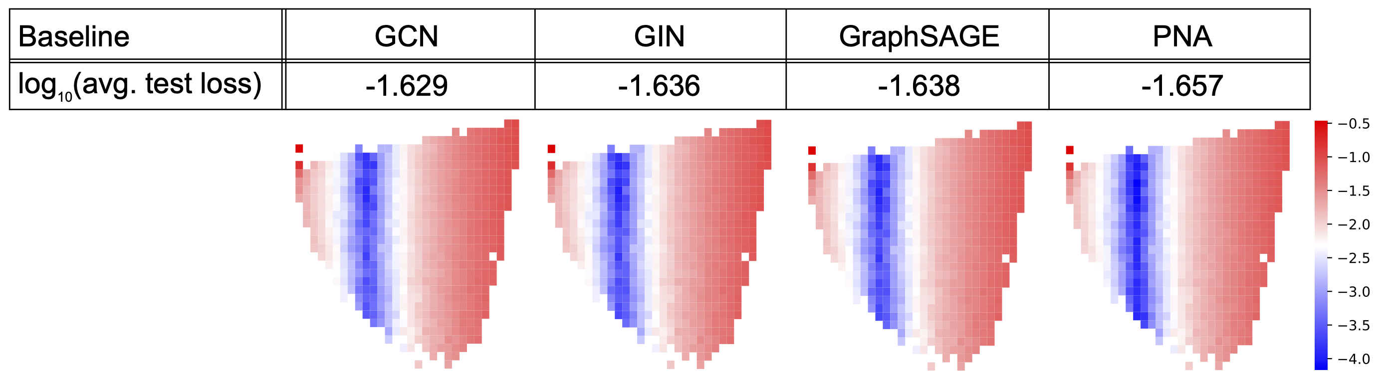
Figure A2: Generalization pattern in graph theory multitask observed from other GNN baseline models, when trained on $\mathcal{G}_{2}$.

• GCN (Kipf & Welling, 2016):

  $$\textbf{h}^{\prime}_{v} = \max_{u\in\mathcal{N}(v)\cup\{u\}}\frac{1}{\sqrt{|\mathcal{N}(v)||\mathcal{N}(u)|}}\textbf{h}_{u}^{(l)}W^{(l)}$$ (7)

• GIN (Xu et al., 2019):

  $$\mathbf{h}^{\prime}_{v} = \sigma\left((1+\epsilon)\cdot\mathbf{h}^{(l)}_{v}+\max_{u\in\mathcal{N}(v)}\mathbf{h}^{(l)}_{u}\right)$$ (8)

• GraphSAGE (Hamilton et al., 2017a):

  $$\mathbf{h}^{\prime}_{v} = \mathbf{W}_{1}\cdot\mathbf{h}^{(l)}_{v}+\mathbf{W}_{2}\cdot\max_{u\in\mathcal{N}(v)}\mathbf{h}^{(l)}_{u}$$ (9)

• PNA (Corso et al., 2020):

  $$\mathbf{h}^{\prime}_{v} = \underset{u\in\mathcal{N}(v)}{\bigoplus}\mathbf{MLP}\left(\mathbf{h}^{(l)}_{u},\mathbf{h}^{(l)}_{v}\right)$$ (10)

  $$\text{where }\bigoplus = \underbrace{\begin{bmatrix}1\\ S(\mathbf{D},\alpha=1)\\ S(\mathbf{D},\alpha=-1)\end{bmatrix}}_{\text{scalers}}\otimes\underbrace{\begin{bmatrix}\mu\\ \sigma\\ \max\\ \min\end{bmatrix}}_{\text{aggregators}}$$ (11)

Figure A3: Message analysis from graph theory multitask.

A.4 BOUNCEGRAD algorithm

When implementing the meta-learning method, it is essential to employ an algorithm that can effectively find approximately optimal update module assignment vectors. In this work, we implement a modified version of the BounceGrad algorithm (Alet et al., 2018) for the graph structured data, which takes the following inputs: a sample space $\mathbb{A}$ of update module assignments, a set of graphs $\mathbb{G}$, a set of network weights $\Theta$, a learning rate $\eta$, a temperature $T$, and a rate of change in temperature $\alpha\in(0,1)$. As in the paper (Alet et al., 2018), we use simulated annealing, a local search algorithm involving stochasticity.

The algorithm begins with initializing the Simulated Annealing running accuracy rate (${\text{SA}}_{r}$) and factor (${\text{SA}}_{f}$). In the main loop, the temperature is updated by the ScheduleTemp procedure based on the current step, the rate of change in temperature $\alpha$, the ${\text{SA}}_{r}$, and the ${\text{SA}}_{f}$. Next, the BOUNCE procedure is called for updating the assignment $\mathcal{A}$. During this step, new assignments $\mathcal{A}^{\prime}$ are proposed for graphs in the mini-batch, and their performance are compared to that of the current assignment using Accept function. The new assignment is accepted when it decreases the loss on the task or, with some probability based on current temperature, even if it does not. Finally, we call the Grad using the assignment to update the network parameters $\Theta$ via the backpropagation algorithm.

To explore the optimal structure of the modules and adapt to new graphs, we run 1000 iterations of meta-test phases for a small number of final training graphs, denoted as $\mathcal{G}_{meta-test}^{train}$. During the meta-testing phase, we rely on the Bounce procedure given a fixed $\Theta$. This approach enables us to find the optimal assignment of the update modules for few-shot meta-test graphs.

Algorithm 1 BounceGrad

1:procedure BounceGrad($\mathbb{A},\mathcal{G}_{train}^{i=1:N},\mathcal{G}_{test}^{i=1:N},\text{SA}_{r},\text{SA}_{f},\eta,T,\alpha$)

2:     $\text{Initialize }\text{SA}_{r},\text{SA}_{f}$

3:     for $i\leftarrow 0$ to $\text{epoch}_{\text{max}}$ do

4:         $T\leftarrow\textsc{ScheduleTemp}(T,i/\text{epoch}_{\text{max}},\alpha,\text{SA}_{r},\text{SA}_{f})$

5:         $\mathcal{A}_{i=1:N},\text{SA}_{r},\text{SA}_{f}\leftarrow\textsc{Bounce}(\mathcal{A}_{i=1:N},\mathcal{G}_{train}^{i=1:N},T,\mathbb{A},\Theta,\text{SA}_{r},\text{SA}_{f})$

6:         $\Theta\leftarrow\textsc{Grad}(\Theta,\mathcal{A}_{i=1:N},\mathcal{G}_{test}^{i=1:N},\eta)$      

Algorithm 2 ScheduleTemp

1:procedure ScheduleTemp($T,step,\alpha,\text{SA}_{r},\text{SA}_{f}$)

2:     $\text{ACC}\leftarrow\exp{(-5*step)}$

3:     if $\text{SA}_{r}/\text{SA}_{f}<\text{ACC}$ then

4:         $T\leftarrow T*\alpha$

5:     else

6:         $T\leftarrow T/\alpha$      return $T$

Algorithm 3 Bounce

1:procedure Bounce($\mathcal{A}_{j=1:N},\mathcal{G}_{train}^{j=1:N},T,\mathbb{A},\Theta,\text{SA}_{r},\text{SA}_{f}$)

2:     for $j\leftarrow 1$ to $N$ do

3:         $\mathcal{A}_{j}^{\prime}\leftarrow$ $\text{Propose}_{\mathbb{A}}$($\mathcal{A}_{j},\Theta$)

4:         $\ell^{\prime}\leftarrow\ell(\mathcal{G}^{j}_{train},\mathcal{A}_{j}^{\prime},\Theta)$

5:         $\ell\leftarrow\ell(\mathcal{G}^{j}_{train},\mathcal{A}_{j},\Theta)$

6:         $f\leftarrow\text{min}(10^{-2},\text{SA}_{r}/\text{SA}_{f})$

7:         if $\text{Accept}(\ell^{\prime},\ell,T)$ then

8:              $\mathcal{A}_{j}\leftarrow\mathcal{A}_{j}^{\prime}$

9:              if $\ell^{\prime}>=\ell$ then

10:                  $\text{SA}_{f}\leftarrow(1-f)*\text{SA}_{f}+f$

11:                  $\text{SA}_{r}\leftarrow(1-f)*\text{SA}_{r}+f$               

12:         else

13:              $\text{SA}_{f}\leftarrow(1-f)*\text{SA}_{f}+f$

14:              $\text{SA}_{r}\leftarrow(1-f)*\text{SA}_{r}$               return $\mathcal{A}_{j=1:N},\text{SA}_{r},\text{SA}_{f}$

Algorithm 4 Accept

1:procedure Accept($\ell,\ell^{\prime},T$)

2:     return $\ell^{\prime}<\ell$ or $\text{rand}(0,1)<\text{exp}\{(\ell-\ell^{\prime})/T\}$

Algorithm 5 Grad

1:procedure Grad($\Theta,\mathcal{A}_{i=1:N},\mathcal{G}_{test}^{i=1:N},\eta$)

2:     $\Delta=0$

3:     for $j\leftarrow 1$ to $N$ do

4:         $(x,y)=$ rand_elt $(\mathcal{G}_{test}^{j})$

5:         $\Delta=\Delta+\nabla_{\Theta}\mathcal{L}(\mathcal{A}_{j\Theta}(x),y)$      

6:     $\Theta=\Theta-\eta\Delta$

7:return $\Theta$

[t] def accept(loss_prev, loss_new, t): """Decide whether to accept the new proposal based on the loss.""" delta = loss_new - loss_prev if loss_new < loss_prev or np.random.rand() < np.exp(-delta / t): return True else: return False

def schedule_temp(s_r, s_f, t): """Update temperature adaptively using a geometric progression.""" acc = np.exp(-5 * epoch / max_epoch) if s_r / s_f < acc: t *= alpha else: t /= alpha return t

def update_parameters(s_r, s_f, f, acceptance): """Update SA parameters based on the success rate.""" s_r = (1.0 - f) * s_r + f if acceptance == True else (1.0 - f) * s_r s_f = (1.0 - f) * s_f + f return s_r, s_f

def bounce(assignment_prev, train_data, T, s_r, s_f, f): """Explore more optimal update module structures using simulated annealing.""" x, y = train_data.x, train_data.y assignment_new = propose(assignment_prev) # Propose a new update module structure. out1, out2 = model(x, a_prev), model(x, a_new) # Evaluate the current and proposed structures. if accept(loss(out1, y), loss(out2, y), T): if loss(out2, y) >= loss(out1, y): s_r, s_f = update_parameters(s_r, s_f, f, True) else: assignment_new = assignment_prev s_r, s_f = update_parameters(s_r, s_f, f, False) return assignment_new, s_r, s_f

def grad(assignment, test_data): """Update model weights based on the test graphs.""" x, y = test_data.x, test_data.y out = model(x, assignment) loss(out, y).backward()

# Initialize update module assignment. assignment = np.random.choice([0, 1], size=(n, num_nodes)) # Loop over minibatches for train_data, test_data in zip(train_loader, test_loader): T = schedule_temp(s_r, s_f, T) # Update SA temperature. # Explore alternative module structures (bounce) and assess their effectiveness (grad). assignment, s_r, s_f = bounce(assignment, train_data, T, s_r, s_f, min(0.01, s_r / s_f)) grad(assignment, test_data)

A.5 Details for real-world graph benchmark

The configurations for the CLRS and GOOD benchmark datasets are presented in Tables A4 and A4, respectively. Additionally, the average node degree distributions are compared among the training, validation, and testing graphs for each real-world graph benchmark (Figure A4). It is worth noting that the structural properties of most benchmark graphs are not clearly distinguishable, as shown in Figure 2d.

Figure A4: Normalized node degree histograms from CLRS and GOOD benchmarks.

A.6 Complete numerical results for CLRS benchmark

Prior research (Mahdavi et al., 2023) has been referred to create our experimental setup, which suggests that disabling hint trajectories can lead to improved performance. When hints are disabled, two algorithms from the same category exhibit identical behavior. As a result, the number of tasks has been reduced from 30 to 24 by choosing one from each algorithmic category. To expedite convergence and facilitate training, we use random scalars in conjunction with deterministic positional indices as node features. Our experiments are repeated three times, and the results are averaged over three random seeds. Table 2 presents the average test scores for all 24 algorithmic tasks, while Table A5 provides the mean and standard deviation for individual tasks.

Table A5: Complete test accuracy (%) of MPNN and three multi-module GNN strategies on CLRS benchmark over 24 algorithmic reasoning tasks.

Algorithms	MPNN	Sigmoid-G	Binary-G	Meta-L
Activity Selector	69.11 $\pm$ 14.67	65.68 $\pm$ 13.56	87.74 $\pm$ 4.90	71.02 $\pm$ 1.69
Articulation Points	95.82 $\pm$ 0.58	96.41 $\pm$ 0.79	97.01 $\pm$ 0.38	96.75 $\pm$ 0.48
Bellman-Ford	98.60 $\pm$ 0.33	98.70 $\pm$ 0.39	98.36 $\pm$ 0.33	71.02 $\pm$ 0.00
BFS	99.97 $\pm$ 0.03	99.93 $\pm$ 0.03	99.98 $\pm$ 0.03	100.00 $\pm$ 0.00
Binary Search	92.46 $\pm$ 1.56	91.88 $\pm$ 1.12	93.88 $\pm$ 2.13	89.79 $\pm$ 2.13
Bridges	59.51 $\pm$ 11.75	56.67 $\pm$ 4.52	87.36 $\pm$ 6.02	75.41 $\pm$ 8.60
DAG Shortest Paths	99.22 $\pm$ 0.27	99.28 $\pm$ 0.20	99.54 $\pm$ 0.20	99.17 $\pm$ 0.08
DFS	25.46 $\pm$ 1.27	24.66 $\pm$ 2.83	27.65 $\pm$ 1.67	25.63 $\pm$ 2.75
Find Max. Subarray	28.74 $\pm$ 5.94	24.48 $\pm$ 1.82	27.05 $\pm$ 1.29	23.76 $\pm$ 2.54
Floyd-Warshall	31.28 $\pm$ 1.55	29.29 $\pm$ 1.02	31.18 $\pm$ 1.49	27.78 $\pm$ 0.63
Graham Scan	99.00 $\pm$ 0.07	99.04 $\pm$ 0.31	98.90 $\pm$ 0.12	98.80 $\pm$ 0.52
LCS Length	58.45 $\pm$ 1.55	58.92 $\pm$ 1.30	60.08 $\pm$ 2.29	58.53 $\pm$ 0.93
Matrix Chain Order	81.13 $\pm$ 3.99	77.10 $\pm$ 3.92	81.55 $\pm$ 5.61	79.74 $\pm$ 2.81
Minimum	99.64 $\pm$ 0.20	99.59 $\pm$ 0.11	99.40 $\pm$ 0.10	99.04 $\pm$ 0.30
MST-Kruskal	59.82 $\pm$ 1.13	61.65 $\pm$ 1.95	61.71 $\pm$ 3.03	59.49 $\pm$ 0.87
MST-Prim	83.28 $\pm$ 0.71	82.88 $\pm$ 1.37	82.88 $\pm$ 1.59	79.67 $\pm$ 1.54
Naïve String Match	10.69 $\pm$ 1.95	10.71 $\pm$ 4.04	21.70 $\pm$ 8.88	5.31 $\pm$ 1.40
Optimal BST	73.92 $\pm$ 2.10	73.20 $\pm$ 1.29	71.34 $\pm$ 5.18	70.14 $\pm$ 2.35
Quickselect	0.00 $\pm$ 0.00	2.51 $\pm$ 4.34	8.61 $\pm$ 8.21	0.00 $\pm$ 0.00
Quicksort	8.15 $\pm$ 2.74	8.38 $\pm$ 4.42	12.68 $\pm$ 2.45	19.06 $\pm$ 4.92
Segments Intersect	98.52 $\pm$ 0.10	98.47 $\pm$ 0.29	98.52 $\pm$ 0.16	98.18 $\pm$ 0.11
SCC	72.49 $\pm$ 0.60	73.81 $\pm$ 1.18	71.26 $\pm$ 1.30	72.79 $\pm$ 0.56
Task Scheduling	83.98 $\pm$ 0.82	83.33 $\pm$ 0.47	83.87 $\pm$ 0.40	83.50 $\pm$ 0.46
Topological Sort	83.92 $\pm$ 1.21	83.85 $\pm$ 0.65	81.65 $\pm$ 2.81	85.08 $\pm$ 1.66
Overall average	67.22	66.68	70.16	67.38

A.7 Complete numerical results for Graph Out-Of-Distribution (GOOD) benchmark

The GOOD benchmark comprises several real-world graph datasets that exhibit unique domain shifts. It provides covariate and concept shifts by altering the input distributions and target distribution, respectively, between the training and testing data. Each dataset contains domain-specific shifts, such as graph size and scaffold in molecular graphs, that cover both types of distribution shifts. Some datasets have no shift, representing the original dataset. Our study focuses solely on graph prediction tasks, as the node-level tasks are based on a single graph (i.e., transductive setting), which is beyond the scope of our research aimed at investigating the ability to generalize to unseen graphs across multiple graphs. The tables A6-A16 below provide information on the mean and standard deviation of OOD generalization performance for each domain shift from the MPNN baseline, multi-module GNNs, and existing OOD methods (IRM and VREx). For more detailed information, please refer to Gui et al. (2022).

Table A6: OOD performance on 27 datasets. All numerical results are averages across 3 random runs. Numbers in bold represent the best results.

Dataset	CLRS $\uparrow$	GOOD-CMNIST $\uparrow$			GOOD-Motif $\uparrow$					GOOD-ZINC $\downarrow$
Metric	Accuracy	Accuracy			Accuracy					MAE
Domain	-	color			base			size		scaffold			size
Dist. shift	-	covariate	concept	no shift	covariate	concept	no shift	covariate	concept	covariate	concept	no shift	covariate	concept
Aggregation	max	max	sum	sum	sum	sum	sum	sum	sum	max	max	max	max	max
MPNN	67.22	35.34	77.57	92.93	63.68	86.94	92.53	57.32	72.87	0.3307	0.2186	0.1731	0.6297	0.2488
Sigmoid-G	66.68	34.71	66.99	91.90	58.43	87.17	92.57	53.29	72.19	0.3163	0.2182	0.1684	0.6421	0.2452
Binary-G	70.16	49.22	74.23	92.56	59.22	87.77	92.52	52.24	71.91	0.3146	0.2178	0.1719	0.6467	0.2506
Meta-L	67.38	43.61	77.53	92.61	76.48	87.17	92.45	58.69	73.38	0.3288	0.2285	0.1791	0.6696	0.2603
IRM	-	41.97	76.45	92.61	68.07	87.33	92.48	56.14	73.61	0.3088	0.2207	0.1717	0.6338	0.2480
VREx	-	45.58	73.83	92.80	73.73	87.69	92.53	59.72	74.07	0.3158	0.2182	0.1723	0.6300	0.2429

Dataset	GOOD-SST2 $\uparrow$			GOOD-PCBA $\uparrow$					GOOD-HIV $\uparrow$					# of tasks with the best results
Metric	Accuracy			Average Precision					ROC-AUC
Domain	length			scaffold			size		scaffold			size
Dist. shift	covariate	concept	no shift	covariate	concept	no shift	covariate	concept	covariate	concept	no shift	covariate	concept
Aggregation	sum	max	max	sum	sum	sum	max	sum	max	sum	max	sum	max
MPNN	80.74	68.27	90.03	11.71	17.71	26.51	11.74	12.04	68.93	63.09	79.70	57.53	70.90	6/27	6/27
Sigmoid-G	80.45	65.79	90.16	11.70	17.89	27.02	10.95	11.56	65.20	63.54	78.73	59.05	71.32	4/27	13/27
Binary-G	80.83	66.69	90.14	11.84	17.98	25.56	10.87	11.98	64.83	63.82	79.15	57.03	70.00	5/27
Meta-L	81.26	67.60	90.22	12.13	16.99	25.81	10.80	11.01	67.79	65.91	79.24	55.50	69.47	4/27
IRM	79.79	65.82	90.09	11.92	17.41	26.31	11.64	11.65	65.07	62.15	78.42	62.22	70.27	2/26	8/26
VREx	78.98	67.30	90.14	12.24	16.25	26.91	11.75	11.95	68.02	63.23	79.97	56.73	70.20	6/26

Table A7: Performance on GOOD-CMNIST with color domain

Accuracy	Aggregation	MPNN	Sigmoid-G	Binary-G	Meta-L	IRM	VREx
covariate	max	35.34 $\pm$ 15.01	34.71 $\pm$ 11.14	49.22 $\pm$ 3.85	43.61 $\pm$ 29.35	41.97 $\pm$ 18.06	45.58 $\pm$ 12.32
concept	sum	77.57 $\pm$ 0.72	66.99 $\pm$ 6.78	74.23 $\pm$ 0.74	77.53 $\pm$ 0.61	76.45 $\pm$ 1.38	73.83 $\pm$ 4.61
no shift	sum	92.93 $\pm$ 0.11	91.90 $\pm$ 0.83	92.56 $\pm$ 0.09	92.61 $\pm$ 0.15	92.61 $\pm$ 0.46	92.80 $\pm$ 0.17

Table A8: Performance on GOOD-Motif with base domain

Accuracy	Aggregation	MPNN	Sigmoid-G	Binary-G	Meta-L	IRM	VREx
covariate	sum	63.68 $\pm$ 2.50	58.43 $\pm$ 0.76	59.22 $\pm$ 1.75	76.48 $\pm$ 3.61	68.07 $\pm$ 2.48	73.73 $\pm$ 6.48
concept	sum	86.94 $\pm$ 0.69	87.17 $\pm$ 0.62	87.77 $\pm$ 1.14	87.17 $\pm$ 1.62	87.33 $\pm$ 0.25	87.69 $\pm$ 1.04

Table A9: Performance on GOOD-Motif with size domain

Accuracy	Aggregation	MPNN	Sigmoid-G	Binary-G	Meta-L	IRM	VREx
covariate	sum	57.32 $\pm$ 4.55	53.29 $\pm$ 4.06	52.24 $\pm$ 2.76	58.69 $\pm$ 12.37	56.14 $\pm$ 4.57	59.72 $\pm$ 3.78
concept	sum	72.87 $\pm$ 0.88	72.19 $\pm$ 2.45	71.91 $\pm$ 0.34	73.38 $\pm$ 2.43	73.61 $\pm$ 1.94	74.07 $\pm$ 2.04
no shift	sum	92.53 $\pm$ 0.01	92.57 $\pm$ 0.00	92.52 $\pm$ 0.08	92.45 $\pm$ 0.08	92.48 $\pm$ 0.07	92.53 $\pm$ 0.04

Table A10: Performance on GOOD-ZINC with scaffold domain

MAE	Aggregation	MPNN	Sigmoid-G	Binary-G	Meta-L	IRM	VREx
covariate	max	0.3307 $\pm$ 0.0076	0.3163 $\pm$ 0.0041	0.3146 $\pm$ 0.0043	0.3288 $\pm$ 0.0110	0.3088 $\pm$ 0.0001	0.3158 $\pm$ 0.0034
concept	max	0.2186 $\pm$ 0.0004	0.2182 $\pm$ 0.0036	0.2178 $\pm$ 0.0016	0.2285 $\pm$ 0.0041	0.2207 $\pm$ 0.0001	0.2182 $\pm$ 0.0001
no shift	max	0.1731 $\pm$ 0.0020	0.1684 $\pm$ 0.0027	0.1719 $\pm$ 0.0019	0.1791 $\pm$ 0.0010	0.1717 $\pm$ 0.0001	0.1723 $\pm$ 0.0011

Table A11: Performance on GOOD-ZINC with size domain

MAE	Aggregation	MPNN	Sigmoid-G	Binary-G	Meta-L	IRM	VREx
covariate	max	0.6297 $\pm$ 0.0134	0.6421 $\pm$ 0.0026	0.6467 $\pm$ 0.0045	0.6696 $\pm$ 0.0107	0.6338 $\pm$ 0.0092	0.6300 $\pm$ 0.0001
concept	max	0.2488 $\pm$ 0.0040	0.2452 $\pm$ 0.0027	0.2506 $\pm$ 0.0030	0.2603 $\pm$ 0.0079	0.2480 $\pm$ 0.0034	0.2429 $\pm$ 0.0001

Table A12: Performance on GOOD-SST2 with length domain

Accuracy	Aggregation	MPNN	Sigmoid-G	Binary-G	Meta-L	IRM	VREx
covariate	sum	80.74 $\pm$ 0.44	80.45 $\pm$ 0.87	80.83 $\pm$ 1.28	81.26 $\pm$ 1.19	79.79 $\pm$ 0.56	78.98 $\pm$ 2.99
concept	max	68.27 $\pm$ 1.76	65.79 $\pm$ 0.64	66.69 $\pm$ 0.95	67.60 $\pm$ 1.86	65.82 $\pm$ 0.00	67.30 $\pm$ 0.40
no shift	max	90.03 $\pm$ 0.18	90.16 $\pm$ 0.14	90.14 $\pm$ 0.01	90.22 $\pm$ 0.18	90.09 $\pm$ 0.00	90.14 $\pm$ 0.08

Table A13: Performance on GOOD-PCBA with scaffold domain

AP	Aggregation	MPNN	Sigmoid-G	Binary-G	Meta-L	IRM	VREx
covariate	sum	11.71 $\pm$ 0.09	11.70 $\pm$ 0.35	11.84 $\pm$ 0.26	12.13 $\pm$ 0.07	11.92 $\pm$ 0.22	12.24 $\pm$ 0.16
concept	sum	17.71 $\pm$ 0.55	17.89 $\pm$ 0.54	17.98 $\pm$ 1.03	16.99 $\pm$ 0.71	17.41 $\pm$ 0.63	16.25 $\pm$ 1.24
no shift	sum	26.51 $\pm$ 0.96	27.02 $\pm$ 0.50	25.56 $\pm$ 1.28	25.81 $\pm$ 0.51	26.31 $\pm$ 0.68	26.91 $\pm$ 0.87

Table A14: Performance on GOOD-PCBA with size domain

AP	Aggregation	MPNN	Sigmoid-G	Binary-G	Meta-L	IRM	VREx
covariate	max	11.74 $\pm$ 0.40	10.95 $\pm$ 0.30	10.87 $\pm$ 0.38	10.80 $\pm$ 0.31	11.64 $\pm$ 0.00	11.75 $\pm$ 0.64
concept	sum	12.04 $\pm$ 0.31	11.56 $\pm$ 0.63	11.98 $\pm$ 0.29	11.01 $\pm$ 0.34	11.65 $\pm$0.68	11.95 $\pm$ 0.30

Table A15: Performance on GOOD-HIV with scaffold domain

ROC-AUC	Aggregation	MPNN	Sigmoid-G	Binary-G	Meta-L	IRM	VREx
covariate	max	68.93 $\pm$ 2.15	65.20 $\pm$ 2.65	64.83 $\pm$ 2.17	67.79 $\pm$ 1.97	65.07 $\pm$ 1.60	68.02 $\pm$ 2.51
concept	sum	63.09 $\pm$ 3.11	63.54 $\pm$ 1.59	63.82 $\pm$ 1.31	65.91 $\pm$ 0.83	62.15 $\pm$ 1.73	63.23 $\pm$ 3.99
no shift	max	79.70 $\pm$ 0.46	78.73 $\pm$ 0.27	79.15 $\pm$ 0.31	79.24 $\pm$ 1.11	78.42 $\pm$ 0.74	79.97 $\pm$ 0.97

Table A16: Performance on GOOD-HIV with size domain

ROC-AUC	Aggregation	MPNN	Sigmoid-G	Binary-G	Meta-L	IRM	VREx
covariate	sum	57.53 $\pm$ 1.89	59.05 $\pm$ 0.92	57.03 $\pm$ 7.18	55.50 $\pm$ 0.33	62.22 $\pm$ 5.02	56.73 $\pm$ 1.47
concept	max	70.90 $\pm$ 2.39	71.32 $\pm$ 1.12	70.00 $\pm$ 0.73	69.47 $\pm$ 0.52	70.27 $\pm$ 2.04	70.20 $\pm$ 0.75

A.8 Effect of module counts and few-shot OOD samples on generalization ability

All experiments in this paper were based on GNNs consisting of two update functions. To explore the impact of an additional update function and exposure to few-shot OOD samples, we trained the multi-module GNNs on $\mathcal{G}_{2}$ in graph theory multitask problem. Our results indicate that although the overall prediction accuracy remained unchanged, the generalization range could become wider. Consequently, we used a two-sample $F$-test to evaluate if there was a statistically significant difference in the variance of the average degree histogram between the single-module GNN baseline and the multi-module GNN histogram. Table A17 confirms that only the meta-learning-based GNN model increases the generalization scope, possibly because of the meta-testing phase’s ability to reuse and restructure module assignment to adapt to a new environment. This finding suggests that multi-module GNNs with meta-learning are more advantageous when given access to a few instances from a novel environment, even if they do not match the OOD setting completely.

Figure A5: The degree distribution of high-performing test graphs when GNNs are trained on $\mathcal{G}_{2}$ is analyzed by fitting a Mixture of Gaussians. The resulting curves are presented in varying colors corresponding to the type of GNNs used. The curves on the left indicate rejection of the null hypothesis at a 5% significance level according to two-sample $F$-test. On the right, it is shown that the variance of the node degree distributions obtained by meta-learning-based GNNs differs from the baseline.

Table A17: $p$-value and test decision for two-sample $F$-test for each model configuration.

Two-sample	sigmoid gating	sigmoid-gating	binary-gating	binary-gating	meta-learning	meta-learning
F-test	(2 modules)	(3 modules)	(2 modules)	(3 modules)	(2 modules)	(3 modules)
$p$-value	0.47	1.0	0.48	0.48	1.66e-29	6.69e-13
$H_{a}:\sigma^{2}=\sigma^{2}_{0}$	True	True	True	True	False	False

References

- Ahuja et al. (2021) Kartik Ahuja, Ethan Caballero, Dinghuai Zhang, Jean-Christophe Gagnon-Audet, Yoshua Bengio, Ioannis Mitliagkas, and Irina Rish. Invariance principle meets information bottleneck for out-of-distribution generalization. Advances in Neural Information Processing Systems, 34:3438–3450, 2021.
- Albert & Barabási (2002) Réka Albert and Albert-László Barabási. Statistical mechanics of complex networks. Reviews of modern physics, 74(1):47, 2002.
- Alet et al. (2018) Ferran Alet, Tomás Lozano-Pérez, and Leslie P Kaelbling. Modular meta-learning. In Conference on Robot Learning, pp. 856–868, 2018.
- Andreas et al. (2016) Jacob Andreas, Marcus Rohrbach, Trevor Darrell, and Dan Klein. Neural module networks. In Proceedings of the IEEE Conference on Computer Vision and Pattern Recognition, pp. 39–48, 2016.
- Arjovsky et al. (2019) Martin Arjovsky, Léon Bottou, Ishaan Gulrajani, and David Lopez-Paz. Invariant risk minimization. arXiv preprint arXiv:1907.02893, 2019.
- Ba et al. (2016) Jimmy Lei Ba, Jamie Ryan Kiros, and Geoffrey E Hinton. Layer normalization. arXiv preprint arXiv:1607.06450, 2016.
- Battaglia et al. (2018) Peter W Battaglia, Jessica B Hamrick, Victor Bapst, Alvaro Sanchez-Gonzalez, Vinicius Zambaldi, Mateusz Malinowski, Andrea Tacchetti, David Raposo, Adam Santoro, Ryan Faulkner, et al. Relational inductive biases, deep learning, and graph networks. arXiv preprint arXiv:1806.01261, 2018.
- Bevilacqua et al. (2021) Beatrice Bevilacqua, Yangze Zhou, and Bruno Ribeiro. Size-invariant graph representations for graph classification extrapolations. In International Conference on Machine Learning, pp. 837–851. PMLR, 2021.
- Bordelon & Pehlevan (2022) Blake Bordelon and Cengiz Pehlevan. Population codes enable learning from few examples by shaping inductive bias. Elife, 11:e78606, 2022.
- Bronstein et al. (2017) Michael M Bronstein, Joan Bruna, Yann LeCun, Arthur Szlam, and Pierre Vandergheynst. Geometric deep learning: Going beyond euclidean data. IEEE Signal Processing Magazine, 34(4):18–42, 2017.
- Chen et al. (2022) Yongqiang Chen, Yonggang Zhang, Yatao Bian, Han Yang, MA Kaili, Binghui Xie, Tongliang Liu, Bo Han, and James Cheng. Learning causally invariant representations for out-of-distribution generalization on graphs. Advances in Neural Information Processing Systems, 35:22131–22148, 2022.
- Chien et al. (2021) Eli Chien, Jianhao Peng, Pan Li, and Olgica Milenkovic. Adaptive universal generalized pagerank graph neural network. In International Conference on Learning Representations, 2021.
- Corso et al. (2020) Gabriele Corso, Luca Cavalleri, Dominique Beaini, Pietro Liò, and Petar Veličković. Principal neighbourhood aggregation for graph nets. Advances in Neural Information Processing Systems, 33:13260–13271, 2020.
- Douglas & Martin (1991) Rodney J Douglas and KA Martin. A functional microcircuit for cat visual cortex. The Journal of Physiology, 440(1):735–769, 1991.
- Duvenaud et al. (2015) David K Duvenaud, Dougal Maclaurin, Jorge Iparraguirre, Rafael Bombarell, Timothy Hirzel, Alán Aspuru-Guzik, and Ryan P Adams. Convolutional networks on graphs for learning molecular fingerprints. In Advances in Neural Information Processing Systems, pp. 2224–2232, 2015.
- Dwivedi et al. (2020) Vijay Prakash Dwivedi, Chaitanya K Joshi, Thomas Laurent, Yoshua Bengio, and Xavier Bresson. Benchmarking graph neural networks. arXiv preprint arXiv:2003.00982, 2020.
- Eliasof et al. (2022) Moshe Eliasof, Eldad Haber, and Eran Treister. pathgcn: Learning general graph spatial operators from paths. In International Conference on Machine Learning, pp. 5878–5891, 2022.
- Ellis et al. (2018) Kevin Ellis, Lucas Morales, Mathias Sablé-Meyer, Armando Solar-Lezama, and Josh Tenenbaum. Learning libraries of subroutines for neurally–guided bayesian program induction. In Advances in Neural Information Processing Systems, volume 31, 2018.
- Erdos et al. (1960) Paul Erdos, Alfréd Rényi, et al. On the evolution of random graphs. Publ. Math. Inst. Hung. Acad. Sci, 5(1):17–60, 1960.
- Fan et al. (2022) Shaohua Fan, Xiao Wang, Yanhu Mo, Chuan Shi, and Jian Tang. Debiasing graph neural networks via learning disentangled causal substructure. In Advances in Neural Information Processing Systems, 2022.
- Feng et al. (2020) Wenzheng Feng, Jie Zhang, Yuxiao Dong, Yu Han, Huanbo Luan, Qian Xu, Qiang Yang, Evgeny Kharlamov, and Jie Tang. Graph random neural networks for semi-supervised learning on graphs. Advances in Neural Information Processing Systemseural information processing systems, 33:22092–22103, 2020.
- Finn et al. (2017) Chelsea Finn, Pieter Abbeel, and Sergey Levine. Model-agnostic meta-learning for fast adaptation of deep networks. In International Conference on Machine Learning, pp. 1126–1135. PMLR, 2017.
- Gainza et al. (2020) Pablo Gainza, Freyr Sverrisson, Frederico Monti, Emanuele Rodola, D Boscaini, MM Bronstein, and BE Correia. Deciphering interaction fingerprints from protein molecular surfaces using geometric deep learning. Nature Methods, 17(2):184–192, 2020.
- Garg et al. (2020) Vikas Garg, Stefanie Jegelka, and Tommi Jaakkola. Generalization and representational limits of graph neural networks. In International Conference on Machine Learning, pp. 3419–3430. PMLR, 2020.
- Geman & Geman (1984) Stuart Geman and Donald Geman. Stochastic relaxation, gibbs distributions, and the bayesian restoration of images. IEEE Transactions on pattern analysis and machine intelligence, (6):721–741, 1984.
- Gilmer et al. (2017) Justin Gilmer, Samuel S Schoenholz, Patrick F Riley, Oriol Vinyals, and George E Dahl. Neural message passing for quantum chemistry. arXiv preprint arXiv:1704.01212, 2017.
- Glorot & Bengio (2010) Xavier Glorot and Yoshua Bengio. Understanding the difficulty of training deep feedforward neural networks. In AISTATS, pp. 249–256, 2010.
- Gui et al. (2022) Shurui Gui, Xiner Li, Limei Wang, and Shuiwang Ji. GOOD: A graph out-of-distribution benchmark. In Thirty-sixth Conference on Neural Information Processing Systems Datasets and Benchmarks Track, 2022.
- Hamilton et al. (2017a) Will Hamilton, Zhitao Ying, and Jure Leskovec. Inductive representation learning on large graphs. Advances in Neural Information Processing Systems, 30, 2017a.
- Hamilton et al. (2017b) William L Hamilton, Rex Ying, and Jure Leskovec. Representation learning on graphs: Methods and applications. IEEE Data Engineering Bulletin, 2017b.
- Han et al. (2022) Xiaotian Han, Zhimeng Jiang, Ninghao Liu, and Xia Hu. G-mixup: Graph data augmentation for graph classification. In International Conference on Machine Learning, pp. 8230–8248. PMLR, 2022.
- Harary (1962) Frank Harary. The maximum connectivity of a graph. Proceedings of the National Academy of Sciences, 48(7):1142–1146, 1962.
- He et al. (2015) Kaiming He, Xiangyu Zhang, Shaoqing Ren, and Jian Sun. Delving deep into rectifiers: Surpassing human-level performance on imagenet classification. In Proceedings of the IEEE international conference on computer vision, pp. 1026–1034, 2015.
- Hu et al. (2020) Weihua Hu, Matthias Fey, Marinka Zitnik, Yuxiao Dong, Hongyu Ren, Bowen Liu, Michele Catasta, and Jure Leskovec. Open graph benchmark: Datasets for machine learning on graphs. Advances in Neural Information Processing Systems, 33:22118–22133, 2020.
- Ioffe & Szegedy (2015) Sergey Ioffe and Christian Szegedy. Batch normalization: Accelerating deep network training by reducing internal covariate shift. In International Conference on Machine Learning, pp. 448–456. pmlr, 2015.
- Jang et al. (2017) Eric Jang, Shixiang Gu, and Ben Poole. Categorical reparameterization with gumbel-softmax. In International Conference on Learning Representations, 2017.
- Kipf & Welling (2016) Thomas N Kipf and Max Welling. Semi-supervised classification with graph convolutional networks. In International Conference on Learning Representations, 2016.
- Kong et al. (2022) Kezhi Kong, Guohao Li, Mucong Ding, Zuxuan Wu, Chen Zhu, Bernard Ghanem, Gavin Taylor, and Tom Goldstein. Robust optimization as data augmentation for large-scale graphs. In Proceedings of the IEEE/CVF Conference on Computer Vision and Pattern Recognition, pp. 60–69, 2022.
- Krueger et al. (2021) David Krueger, Ethan Caballero, Joern-Henrik Jacobsen, Amy Zhang, Jonathan Binas, Dinghuai Zhang, Remi Le Priol, and Aaron Courville. Out-of-distribution generalization via risk extrapolation (rex). In International Conference on Machine Learning, pp. 5815–5826. PMLR, 2021.
- Li et al. (2021) Haoyang Li, Xin Wang, Ziwei Zhang, Zehuan Yuan, Hang Li, and Wenwu Zhu. Disentangled contrastive learning on graphs. Advances in Neural Information Processing Systems, 34:21872–21884, 2021.
- Li et al. (2022a) Haoyang Li, Ziwei Zhang, Xin Wang, and Wenwu Zhu. Disentangled graph contrastive learning with independence promotion. IEEE Transactions on Knowledge and Data Engineering, 2022a.
- Li et al. (2022b) Haoyang Li, Ziwei Zhang, Xin Wang, and Wenwu Zhu. Learning invariant graph representations for out-of-distribution generalization. In Advances in Neural Information Processing Systems, 2022b.
- Li et al. (2015) Yujia Li, Daniel Tarlow, Marc Brockschmidt, and Richard Zemel. Gated graph sequence neural networks. arXiv preprint arXiv:1511.05493, 2015.
- Liu et al. (2022) Songtao Liu, Rex Ying, Hanze Dong, Lanqing Li, Tingyang Xu, Yu Rong, Peilin Zhao, Junzhou Huang, and Dinghao Wu. Local augmentation for graph neural networks. In International Conference on Machine Learning, pp. 14054–14072. PMLR, 2022.
- Liu et al. (2020) Yanbei Liu, Xiao Wang, Shu Wu, and Zhitao Xiao. Independence promoted graph disentangled networks. In Proceedings of the AAAI Conference on Artificial Intelligence, volume 34, pp. 4916–4923, 2020.
- Lu et al. (2021) Chaochao Lu, Yuhuai Wu, José Miguel Hernández-Lobato, and Bernhard Schölkopf. Invariant causal representation learning for out-of-distribution generalization. In International Conference on Learning Representations, 2021.
- Luan et al. (2020) Sitao Luan, Mingde Zhao, Chenqing Hua, Xiao-Wen Chang, and Doina Precup. Complete the missing half: Augmenting aggregation filtering with diversification for graph convolutional networks. arXiv preprint arXiv:2008.08844, 2020.
- Luan et al. (2022) Sitao Luan, Chenqing Hua, Qincheng Lu, Jiaqi Zhu, Mingde Zhao, Shuyuan Zhang, Xiao-Wen Chang, and Doina Precup. Revisiting heterophily for graph neural networks. In S. Koyejo, S. Mohamed, A. Agarwal, D. Belgrave, K. Cho, and A. Oh (eds.), Advances in Neural Information Processing Systems, volume 35, pp. 1362–1375, 2022.
- Ma et al. (2019) Jianxin Ma, Peng Cui, Kun Kuang, Xin Wang, and Wenwu Zhu. Disentangled graph convolutional networks. In International Conference on Machine Learning, pp. 4212–4221. PMLR, 2019.
- Maddison et al. (2017) Chris J. Maddison, Andriy Mnih, and Yee Whye Teh. The concrete distribution: A continuous relaxation of discrete random variables. In International Conference on Learning Representations, 2017.
- Mahdavi et al. (2023) Sadegh Mahdavi, Kevin Swersky, Thomas Kipf, Milad Hashemi, Christos Thrampoulidis, and Renjie Liao. Towards better out-of-distribution generalization of neural algorithmic reasoning tasks. Transactions on Machine Learning Research, 2023. ISSN 2835-8856.
- Maskey et al. (2022) Sohir Maskey, Ron Levie, Yunseok Lee, and Gitta Kutyniok. Generalization analysis of message passing neural networks on large random graphs. In Advances in Neural Information Processing Systems, 2022.
- Miao et al. (2022) Siqi Miao, Mia Liu, and Pan Li. Interpretable and generalizable graph learning via stochastic attention mechanism. In International Conference on Machine Learning, pp. 15524–15543. PMLR, 2022.
- Morris et al. (2019) Christopher Morris, Martin Ritzert, Matthias Fey, William L Hamilton, Jan Eric Lenssen, Gaurav Rattan, and Martin Grohe. Weisfeiler and leman go neural: Higher-order graph neural networks. In Proceedings of the AAAI Conference on Artificial Intelligence, volume 33, pp. 4602–4609, 2019.
- Morris et al. (2021) Christopher Morris, Yaron Lipman, Haggai Maron, Bastian Rieck, Nils M Kriege, Martin Grohe, Matthias Fey, and Karsten Borgwardt. Weisfeiler and leman go machine learning: The story so far. arXiv preprint arXiv:2112.09992, 2021.
- Murphy et al. (2018) Ryan L Murphy, Balasubramaniam Srinivasan, Vinayak Rao, and Bruno Ribeiro. Janossy pooling: Learning deep permutation-invariant functions for variable-size inputs. In International Conference on Learning Representations, 2018.
- Nichol et al. (2018) Alex Nichol, Joshua Achiam, and John Schulman. On first-order meta-learning algorithms. In CoRR, abs/1803.02999, 2018.
- Ovadia et al. (2019) Yaniv Ovadia, Emily Fertig, Jie Ren, Zachary Nado, David Sculley, Sebastian Nowozin, Joshua Dillon, Balaji Lakshminarayanan, and Jasper Snoek. Can you trust your model’s uncertainty? evaluating predictive uncertainty under dataset shift. Advances in Neural Information Processing Systems, 32, 2019.
- Pakman & Paninski (2013) Ari Pakman and Liam Paninski. Auxiliary-variable exact hamiltonian monte carlo samplers for binary distributions. In Advances in Neural Information Processing Systems, pp. 2490–2498, 2013.
- Park et al. (2021) Hyeonjin Park, Seunghun Lee, Sihyeon Kim, Jinyoung Park, Jisu Jeong, Kyung-Min Kim, Jung-Woo Ha, and Hyunwoo J Kim. Metropolis-hastings data augmentation for graph neural networks. Advances in Neural Information Processing Systems, 34:19010–19020, 2021.
- Pearl (1988) Judea Pearl. Probabilistic Reasoning in Intelligent Systems: Networks of Plausible Inference. Morgan Kaufmann, 1988.
- Pham et al. (2017) Trang Pham, Truyen Tran, Dinh Phung, and Svetha Venkatesh. Column networks for collective classification. In Thirty-first AAAI Conference on Artificial Intelligence, 2017.
- Sanchez-Gonzalez et al. (2018) Alvaro Sanchez-Gonzalez, Nicolas Heess, Jost Tobias Springenberg, Josh Merel, Martin Riedmiller, Raia Hadsell, and Peter Battaglia. Graph networks as learnable physics engines for inference and control. In International Conference on Machine Learning, pp. 4470–4479. PMLR, 2018.
- Sanchez-Gonzalez et al. (2020) Alvaro Sanchez-Gonzalez, Jonathan Godwin, Tobias Pfaff, Rex Ying, Jure Leskovec, and Peter Battaglia. Learning to simulate complex physics with graph networks. In International Conference on Machine Learning, pp. 8459–8468. PMLR, 2020.
- Sato (2020) Ryoma Sato. A survey on the expressive power of graph neural networks. arXiv preprint arXiv:2003.04078, 2020.
- Satorras & Welling (2021) Victor Garcia Satorras and Max Welling. Neural enhanced belief propagation on factor graphs. In International Conference on Artificial Intelligence and Statistics, pp. 685–693. PMLR, 2021.
- Scarselli et al. (2008) Franco Scarselli, Marco Gori, Ah Chung Tsoi, Markus Hagenbuchner, and Gabriele Monfardini. The graph neural network model. IEEE Transactions on Neural Networks, 20(1):61–80, 2008.
- Schmidhuber (1987) Jürgen Schmidhuber. Evolutionary principles in self-referential learning, or on learning how to learn: the meta-meta-… hook. PhD thesis, Technische Universität München, 1987.
- Selsam et al. (2019) Daniel Selsam, Matthew Lamm, Benedikt Bünz, Percy Liang, Leonardo de Moura, and David L Dill. Learning a sat solver from single-bit supervision. In International Conference on Learning Representations, 2019.
- Shepherd (2004) Gordon M Shepherd. The synaptic organization of the brain. Oxford university press, 2004.
- Sui et al. (2022) Yongduo Sui, Xiang Wang, Jiancan Wu, Min Lin, Xiangnan He, and Tat-Seng Chua. Causal attention for interpretable and generalizable graph classification. In Proceedings of the 28th ACM SIGKDD Conference on Knowledge Discovery and Data Mining, pp. 1696–1705, 2022.
- Tenenbaum et al. (2011) Joshua B Tenenbaum, Charles Kemp, Thomas L Griffiths, and Noah D Goodman. How to grow a mind: Statistics, structure, and abstraction. Science, 331(6022):1279–1285, 2011.
- Thrun & Pratt (2012) Sebastian Thrun and Lorien Pratt. Learning to learn. Springer Science & Business Media, 2012.
- Veličković et al. (2018) Petar Veličković, Guillem Cucurull, Arantxa Casanova, Adriana Romero, Pietro Lio, and Yoshua Bengio. Graph attention networks. In International Conference on Learning Representations, 2018.
- Veličković et al. (2022) Petar Veličković, Adrià Puigdomènech Badia, David Budden, Razvan Pascanu, Andrea Banino, Misha Dashevskiy, Raia Hadsell, and Charles Blundell. The clrs algorithmic reasoning benchmark. In International Conference on Machine Learning, pp. 22084–22102. PMLR, 2022.
- Verma et al. (2019) Vikas Verma, Alex Lamb, Christopher Beckham, Amir Najafi, Ioannis Mitliagkas, David Lopez-Paz, and Yoshua Bengio. Manifold mixup: Better representations by interpolating hidden states. In International Conference on Machine Learning, pp. 6438–6447. PMLR, 2019.
- Verma et al. (2021) Vikas Verma, Meng Qu, Kenji Kawaguchi, Alex Lamb, Yoshua Bengio, Juho Kannala, and Jian Tang. Graphmix: Improved training of gnns for semi-supervised learning. In Proceedings of the AAAI conference on artificial intelligence, volume 35, pp. 10024–10032, 2021.
- Wainwright et al. (2003) Martin J Wainwright, Tommi S Jaakkola, and Alan S Willsky. Tree-based reparameterization framework for analysis of sum-product and related algorithms. IEEE Transactions on Information Theory, 49(5):1120–1146, 2003.
- Wang et al. (2020) Yiwei Wang, Wei Wang, Yuxuan Liang, Yujun Cai, Juncheng Liu, and Bryan Hooi. Nodeaug: Semi-supervised node classification with data augmentation. In Proceedings of the 26th ACM SIGKDD International Conference on Knowledge Discovery & Data Mining, pp. 207–217, 2020.
- Wang et al. (2021) Yiwei Wang, Wei Wang, Yuxuan Liang, Yujun Cai, and Bryan Hooi. Mixup for node and graph classification. In Proceedings of the Web Conference 2021, pp. 3663–3674, 2021.
- Watts & Strogatz (1998) Duncan J Watts and Steven H Strogatz. Collective dynamics of ‘small-world’networks. Nature, 393(6684):440–442, 1998.
- Wu et al. (2022a) Lirong Wu, Haitao Lin, Yufei Huang, and Stan Z Li. Knowledge distillation improves graph structure augmentation for graph neural networks. In Advances in Neural Information Processing Systems, 2022a.
- Wu et al. (2022b) Qitian Wu, Hengrui Zhang, Junchi Yan, and David Wipf. Handling distribution shifts on graphs: An invariance perspective. In International Conference on Learning Representations, 2022b.
- Wu et al. (2022c) Yingxin Wu, Xiang Wang, An Zhang, Xiangnan He, and Tat-Seng Chua. Discovering invariant rationales for graph neural networks. In International Conference on Learning Representations, 2022c.
- Xu et al. (2019) Keyulu Xu, Weihua Hu, Jure Leskovec, and Stefanie Jegelka. How powerful are graph neural networks? In International Conference on Learning Representations, 2019.
- Yoon et al. (2018) KiJung Yoon, Renjie Liao, Yuwen Xiong, Lisa Zhang, Ethan Fetaya, Raquel Urtasun, Richard Zemel, and Xaq Pitkow. Inference in probabilistic graphical models by graph neural networks. In arXiv preprint arXiv:1803.07710., 2018.
- You et al. (2020) Jiaxuan You, Jure Leskovec, Kaiming He, and Saining Xie. Graph structure of neural networks. In International Conference on Machine Learning, pp. 10881–10891. PMLR, 2020.
- Zaheer et al. (2017) Manzil Zaheer, Satwik Kottur, Siamak Ravanbakhsh, Barnabas Poczos, Russ R Salakhutdinov, and Alexander J Smola. Deep sets. Advances in Neural Information Processing Systems, 30, 2017.
- Zhang et al. (2018) Hongyi Zhang, Moustapha Cisse, Yann N Dauphin, and David Lopez-Paz. mixup: Beyond empirical risk minimization. In International Conference on Learning Representations, 2018.
- Zhang et al. (2022) Zeyang Zhang, Xin Wang, Ziwei Zhang, Haoyang Li, Zhou Qin, and Wenwu Zhu. Dynamic graph neural networks under spatio-temporal distribution shift. In Advances in Neural Information Processing Systems, 2022.
- Zhao et al. (2021) Tong Zhao, Yozen Liu, Leonardo Neves, Oliver Woodford, Meng Jiang, and Neil Shah. Data augmentation for graph neural networks. In Proceedings of the AAAI Conference on Artificial Intelligence conference on artificial intelligence, volume 35, pp. 11015–11023, 2021.
- Zhou et al. (2022) Yangze Zhou, Gitta Kutyniok, and Bruno Ribeiro. OOD link prediction generalization capabilities of message-passing GNNs in larger test graphs. In Alice H. Oh, Alekh Agarwal, Danielle Belgrave, and Kyunghyun Cho (eds.), Advances in Neural Information Processing Systems, 2022.