Classical Sequence Match is a Competitive Few-Shot One-Class Learner

Abstract

Nowadays, transformer-based models gradually become the “default choice” for artificial intelligence pioneers. The models also show superiority even in the few-shot scenarios. In this paper, we revisit the classical methods and propose a new few-shot alternative. Specifically, we investigate the few-shot one-class problem, which actually takes a known sample as a reference to detect whether an unknown instance belongs to the same class. This problem can be studied from the perspective of sequence match. It is shown that with meta-learning, the classical sequence match method, i.e. Compare-Aggregate, significantly outperforms transformer ones. The classical approach requires much less training cost. Furthermore, we perform an empirical comparison between two kinds of sequence match approaches under simple fine-tuning and meta-learning. Meta-learning causes the transformer models’ features to have high-correlation dimensions. The reason is closely related to the number of layers and heads of transformer models. Experimental codes and data are available at https://github.com/hmt2014/FewOne.

1 Introduction

When the labeled data is scarce in practical application, it is struggled to learn a well-performed model using deep learning algorithms. Yet annotating data costs much labor and time. Few-shot learning (FSL) intuitively addresses this obstacle Koch et al. (2015); Vinyals et al. (2016); Snell et al. (2017); Finn et al. (2017); Sung et al. (2018). FSL learns at the meta-task level, where each meta-task is formulated as inferring queries with the help of a support set Vinyals et al. (2016). Multiple meta-tasks facilitate the task-agnostic transferrable knowledge. Thus it can learn new knowledge fast after being taught only a few samples. Despite FSL has been well-studied, its one-class scenario Frikha et al. (2021) is less investigated.

Figure 1: Meta-task example in few-shot one-class text classification, where 1 denotes a positive instance and 0 denotes a negative one.

In this paper, following the one-class trait, we design each meta-task as a binary classification. It consists of a reference instance, a support set, and a query set (see Figure 1). The reference instance is one known sample of a class, which is exploited to tell whether an instance out of the support/query set belongs to the same class. Such purpose is consistent with sequence match, which also makes a decision for two sequences. Previous sequence match can mainly be categorized into two promising directions: classical methods, e.g. Siamese Network Koch et al. (2015), Compare-Aggregate (CA) Wang and Jiang (2017), and transformer-based method, e.g. DistilBert Sanh et al. (2019), BERT Devlin et al. (2019).

In recent years, transformer models have already beaten classical ones in a wide range of tasks Devlin et al. (2019). We wonder how two kinds of models perform under the few-shot one-class scenario. Consequently, it is presented that with meta-learning, classical sequence match method can significantly outperform transformer-based models. The classical models require much less training cost. Specifically, model-agnostic meta-learning (MAML) algorithm Finn et al. (2017) is a subtle bi-level optimizing approach that aims to learn a good parameter initialization. By introducing this algorithm, classical methods act as simple but competitive few-shot one-class learners.

Furthermore, we make an empirical comparison between classical and transformer-based models under simple fine-tuning and meta-learning. Firstly, it is found that MAML has a more positive impact on the both sequence match approaches than simple fine-tuning. This suggests that a good parameter initialization is important for both of them. Secondly, MAML tends to make transformer models extract features with high-correlation dimensions. The bi-level optimization might cause the feature extraction layers of large models less trained. Yet the last classifying layer tends to be better learned relatively. We demonstrate that the high correlation is related to the number of heads and layers in the transformer.

In summary, our main contributions are as follows: (1) We present a simple but competitive few-shot one-class learner, which is based on the classical sequence match approach and meta-learning. Extensive experimental results show that this learner achieves significant improvements compared with transformer-based models. This provides new insights in the transformer-dominant era. (2) Based on the testbed provided by the above approaches, an empirical study is made to further reveal their underlining natures. New observations and conclusions are derived.

2 Related Works

2.1 Few-Shot Learning

Few-shot learning (FSL) Fei-Fei et al. (2006) deals with the practical problem of data scarcity in an intuitive way. It learns new knowledge fast with limited supervised information. An early work Koch et al. (2015) learns to detect whether two instances belong to the same class. Later, matching network Vinyals et al. (2016) proposes to construct multiple meta-tasks in both the training and testing procedures. This setting becomes mainstream in the subsequent works, to name a few, distance-based methods Snell et al. (2017); Sung et al. (2018); Garcia and Bruna (2018); Bao et al. (2020), optimization-based methods Finn et al. (2017); Munkhdalai and Yu (2017) or hallucination-based methods Wang et al. (2018); Li et al. (2020). Among them, MAML Finn et al. (2017) is special for “model-agnostic”, indicating that this algorithm can be applied in any model. Therefore, we choose to further study its effects. To the best of our knowledge, it is seldom studied in transformer-based models. We provide an interesting empirical analysis in the experiments.

Recently, prompt-based fine-tuning Gao et al. (2021) also become popular in FSL. It classifies a template-based instance through the masked language model. This prediction manner bridges the gap between pre-training and fine-tuning. Its effectiveness in the few-shot one-class scenario is under-explored.

2.2 One-Class Few-Shot Learning

Recently some works discuss the one-class problem in FSL. Cumulative LEARning (CLEAR) Kozerawski and Turk (2018) uses transfer learning to model the decision boundary of SVM. One-way proto (OWP) Kruspe (2019) is based on the prototypical network Snell et al. (2017). OWP computes the positive prototype by simply averaging the representations of instances. It designs a 0-vector as the negative prototype. The Euclidean distance with prototypes in the embedding space indicates that an instance is positive or negative. One-class MAML Frikha et al. (2021) proposes a simple data sampling strategy to ensure that the class-imbalance rate of the inner-level matches the test task. Different from them, we leverage the unique direction in natural language processing, i.e. sequence match, to study the one-class FSL.

2.3 Sequence Match

Sequence match aims to make a decision for two sequences. Many tasks require to match sequences, such as text entailment Bowman et al. (2015), machine comprehension Tapaswi et al. (2016), recommendation Kraus and Feuerriegel (2019), etc. A straightforward approach is to encode each sequence as a vector and then compare the two vectors to make a decision Bowman et al. (2015); Feng et al. (2015). However, a single vector is insufficient to match the important information between two sequences. Thus attention mechanism is adopted in this task Rocktäschel et al. (2016).

Later, the Compare-Aggregate framework is proposed Wang and Jiang (2017) for matching sequences, which has been widely studied. Its extended version usually considers the bidirectional information of two inputs Bian et al. (2017); Yoon et al. (2019). One previous work Ye and Ling (2019) shows that matching and aggregation are effective in few-shot relation classification. We explore this framework in the few-shot one-class problem. More recently, pre-trained language models, e.g. BERT Sanh et al. (2019) gain remarkable achievements in many sequence match tasks Wang et al. (2020).

3 Methods

In this work, two kinds of sequence match methods, including classical and transformer-based ones, are mainly investigated. Compare-Aggregate Wang and Jiang (2017) is a promising classical method. We choose to study its extended version, i.e. Bidirectional Compare-Aggregate (BiCA) Bian et al. (2017); Yoon et al. (2019), introduced in §3.2. The transformer-based sequence match Sanh et al. (2019) is also presented in §3.3 briefly.

3.1 Problem Definition

Assume the training data $\mathcal{D}_{train}$ is composed of a set of training classes $\mathcal{C}_{train}$, and the testing data $\mathcal{D}_{test}$ has a set of classes $\mathcal{C}_{test}$, there are no overlapping between two class sets $\mathcal{C}_{train}\cap{\mathcal{C}_{test}}=\varnothing$. During training, we randomly sample a bunch of meta-tasks from $\mathcal{C}_{train}$. A meta-task is made as a binary classifier to detect one class, which is formulated as below.

A meta-task contains a reference sentence $r$, a support set $S$ and a query set $Q$.

$$\begin{split}S&=\{(x_{s}^{1},y_{s}^{1}),(x_{s}^{2},y_{s}^{2}),...(x_{s}^{|S|},y_{s}^{|S|})\}\\ Q&=\{(x_{q}^{1},y_{q}^{1}),(x_{q}^{2},y_{q}^{2}),...(x_{q}^{|Q|},y_{q}^{|Q|})\}\end{split}$$ (1)

where $x_{s}$/$x_{q}$ is an instance and $y_{s}$/$y_{q}$ denotes whether this instance belongs to the same class as the reference. $|S|$ and $|Q|$ indicate the number of instances in two sets, respectively. Many meta-tasks enable the model to extract task-agnostic knowledge, which is beneficial to the meta-tasks from the testing classes $\mathcal{C}_{test}$.

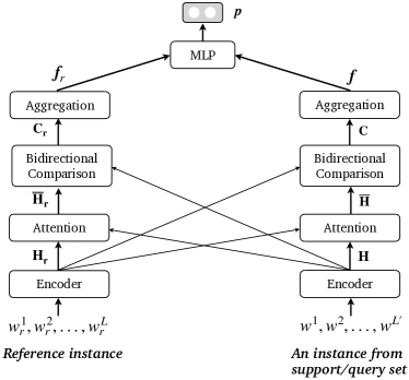
Figure 2: The network architecture of BiCA. The parameters are shared by two input instances.

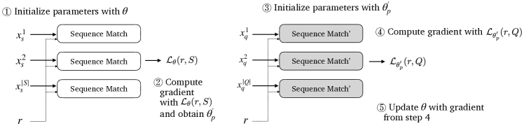
Figure 3: Introducing meta-learning to sequence match approaches. The left part and the right part share the same architecture but employ different parameters in the meta-learning. The five steps are corresponding to the Algorithm 1. After training, the optimal parameter initialization $\theta$ for the testing classes is obtained.

3.2 Classical Sequence Match

In this section, we will introduce the components of Bidirectional Compare-Aggregate (BiCA) in detail.

Encoder   Given an input sentence with $L$ words, denoted as $\{w^{1},w^{2},...,w^{L}\}$, it is first mapped into an embedding sequence $\mathrm{\bf{E}}=\{\bm{e^{1}},\bm{e^{2}},...,\bm{e^{L}}\}$ by looking up the pre-trained GloVe embeddings Pennington et al. (2014). Then the embedding sequence is processed by the gate mechanism Wang and Jiang (2017) to obtain contextualized information. This gating mechanism aims at remembering the meaningful words and filtering the less-important words in a sentence.

$$\mathrm{\bf{H}}=\mathrm{\sigma}(\mathrm{\bf{W^{i}E}}+\bm{b^{i}}){\odot}\mathrm{tanh}(\mathrm{\bf{W^{u}E}}+\bm{b^{u}})$$ (2)

where $\mathrm{\bf{W^{i}}}$ and $\mathrm{\bf{W^{u}}}$ are parameter matrix, $\bm{b^{i}}$ and $\bm{b^{u}}$ are biases, $\odot$ is element-wise multiplication.

Attention   As depicted in Figure 2, the reference and an instance from support/query set are fed into the encoder, obtaining $\mathrm{\bf{H_{r}}}$ and $\mathrm{\bf{H}}$. Then the interaction between two inputs is computed through an attention mechanism.

$$\begin{split}\mathrm{\bf{\overline{H}_{r}}}&=\mathrm{\bf{H_{r}}}\cdot\mathrm{softmax}(\mathrm{\bf{H_{r}}}^{\mathrm{T}}\mathrm{\bf{H}})\\ \mathrm{\bf{\overline{H}}}&=\mathrm{\bf{H}}\cdot\mathrm{softmax}(\mathrm{\bf{H}}^{\mathrm{T}}\mathrm{\bf{H_{r}}})\\ \end{split}$$ (3)

This attention mechanism is non-parametric since it only depends on the encoded representations $\mathrm{\bf{H_{r}}}$ and $\mathrm{\bf{H}}$. Such design reduces the reliance on parameters and focuses on learning the relationships between data. Hence, this helps better adapt to unseen classes.

Bidirectional Comparison   To compare the two instances, we adopt a simple word-level comparison function, i.e., element-wise multiplication $\odot$.

$$\mathrm{\bf{C_{r}}}=\mathrm{\bf{\overline{H}_{r}}}\odot\mathrm{\bf{H}}\;\;\;\;\;\mathrm{\bf{C}}=\mathrm{\bf{\overline{H}}}\odot\mathrm{\bf{H_{r}}}$$ (4)

The comparison function is also non-parametric for the purpose of adaptation. As shown in Figure 2, the encoded representations are applied in both the attention and bidirectional comparison modules to promote the mutual interaction of two inputs.

Aggregation   Following the original work Wang and Jiang (2017), the comparison representations are aggregated by convolution neural network (CNN) Kim (2014). The convolution kernel slides over the comparison sequence to extract $n$-gram features, which tends to be helpful in matching.

$$\bm{f_{r}}=\mathrm{CNN}(\mathrm{\bf{C_{r}}})\;\;\;\;\;\bm{f}=\mathrm{CNN}(\mathrm{\bf{C}})$$ (5)

where $\mathrm{CNN}(\cdot)$ is a convolution operation followed by max-pooling. Then the matching score is computed with the aggregation representations of two input sentences.

$$\bm{p}=\mathrm{MLP}([\bm{f_{r}},\bm{f}])$$ (6)

where $\mathrm{MLP}$ is a single linear layer. $\bm{p}$ is a two-dimensional logits output.

Loss   The training objective of BiCA is the cross entropy loss.

$$\mathcal{L}_{\theta}(r,S)=-\frac{1}{|S|}\sum_{|S|}\mathrm{log}P(y|\bm{p})$$ (7)

where $y$ is the ground truth. $\theta$ represents all the parameters in the sequence match model.

3.3 Transformer-Based Sequence Match

Transformer-based models, e.g. BERT Devlin et al. (2019) are pre-trained on a large-scale corpus, serving as foundational backbones for a wide range of natural language processing tasks. When aiming at sequence match, BERT utilizes two special tokens $\mathtt{[CLS]}$ and $\mathtt{[SEP]}$ to concatenate two sequences as a whole. For the two input instances shown in Figure 2, they are combined into $\{\mathtt{[CLS]},w_{r}^{1},w_{r}^{2},...,w_{r}^{L},\mathtt{[SEP]},w^{1},w^{2},...,w^{L^{\prime}}\}$, where the output of $\mathtt{[CLS]}$ is usually for classification and $\mathtt{[SEP]}$ is for separating two inputs. This combined sequence is then fed into BERT. The self-attention mechanism Vaswani et al. (2017) in the transformer will compute the interaction between two inputs. Finally, the output of the first token $\mathtt{[CLS]}$ is adopted for inference. The training objective is also computed by Eq. (7).

Input: Training data from $\mathcal{D}_{train}$

1 Randomly initialize $\theta$

2 repeat

3       Sample positive classes $\mathcal{C}_{p}$ and negative classes $\mathcal{C}_{n}$ from $\mathcal{D}_{train}$

4       $\mathcal{C}_{p}\cap{\mathcal{C}_{n}}=\varnothing$

5       for all $\mathcal{C}_{p}$ do

6             Construct a meta-task

7             Evaluate $\nabla_{\theta}{\mathcal{L}_{\theta}}(r,S)$ in Eq. (7)

8             Compute adapted parameters with gradient descent: $\theta_{p}^{{}^{\prime}}=\theta-\alpha\nabla_{\theta}{\mathcal{L}_{\theta}(r,S)}$

9            

10      Update $\theta\leftarrow\theta-\beta\nabla_{\theta}\sum_{\mathcal{C}_{p}}{\mathcal{L}_{\theta^{{}^{\prime}}_{p}}(r,Q)}$

11until performance on the validation data set does not improve in 3 epochs.

Algorithm 1 Meta-Learning for Few-Shot One-Class Problem

3.4 Meta-Learning for Sequence Match

In the few-shot one-class paradigm, a meta-task from the unseen class has a few labeled instances as the support set. To better leverage such knowledge, we introduce meta-learning to sequence match models, which is displayed in Figure 3 and Algorithm 1. Specifically, model-agnostic meta-learning (MAML) algorithm Finn et al. (2017) is chosen to investigate its impact on the sequence match approaches. This algorithm learns a good initialization of model parameters by maximizing the sensitivity of the loss function when adapting to new tasks Song et al. (2020).

Construct a Meta-Task   In Algorithm 1 (line 6), given a positive class, we first sample $N+1$ instances from this class, which constitutes a reference instance $r$ and $N$ positive ones. Moreover, $N$ negative examples are also sampled from the negative classes $\mathcal{C}_{n}$. These positive and negative examples are mixed up randomly, which are further divided into the support set and query set.

Meta-learning trains in a bi-level way (see Algorithm 1), including the inner-level (line 8) and the outer-level (line 9) for the support set $S$ and the query set $Q$, respectively. This way will cause the gradients for updating parameters to propagate through more layers (line 9), i.e. twice as many as the number of network layers in a sequence match model. Its special effects on the transformer models are further discussed in §4.4. When evaluating, a model is initialized from the parameters $\theta$ trained by MAML on the training classes, which is then optimized with the support set on the testing classes.

		Train	Validation	Test
Class Num		64	16	20
Data Num	single	13677	3394	4671
	multi	26643	6686	7929
Data Num/Class	single	213.7	212.1	233.5
	multi	416.2	417.8	396.4

Table 1: Dataset statistics for ACD. single denotes the single-aspect sentence and multi denotes the multi-aspect one.

4 Experiments

4.1 Datasets

Aspect Category Detection (ACD)   A dataset for few-shot one-class ACD is collected from YelpAspect Bauman et al. (2017); Li et al. (2019), which is a large-scale multi-domain dataset for fine-grained sentiment analysis. The 100 aspect categories are split without intersection into 64 classes for training, 16 classes for validation, and 20 classes for testing. Table 1 displays the statistics of the dataset. The data in each class is further divided according to the number of the aspects in a sentence, into single-aspect and multi-aspect. Relatively, a multi-aspect example contains more noise when matching sequences. To explore a challenging scenario, the support/query set are both sampled from the multi-aspect set. Fixing this setup, we choose a reference instance as a single- and multi-aspect one.

HuffPost   It consists of news headlines published in HuffPost between 2012 and 2018 Misra (2018); Misra and Grover (2021). Bao et al. (2020) process the original dataset for few-shot text classification. The number of training, validation, and testing classes are 20, 5, and 16, respectively, where each class has 900 instances. Since the sentences are headlines, they are shorter and less grammatical.

Model	Use support	Match Type		ACD Single		ACD Multi		HuffPost
	set of $\mathcal{D}_{test}$	vector	word	Acc	F1	Acc	F1	Acc	F1
SN	No	✓		69.88$\pm$1.19	69.33$\pm$1.16	72.12$\pm$0.82	71.64$\pm$0.82	62.61$\pm$0.55	61.87$\pm$0.56
OWP	No	✓		72.50$\pm$1.22	71.96$\pm$1.23	70.94$\pm$0.58	70.24$\pm$0.65	61.72$\pm$0.72	61.05$\pm$0.72
CA	No		✓	79.45$\pm$1.17	78.97$\pm$1.25	76.72$\pm$0.99	76.27$\pm$0.96	64.02$\pm$0.36	63.33$\pm$0.47
BiCA	No		✓	79.46$\pm$0.39	79.03$\pm$0.46	76.81$\pm$0.89	76.40$\pm$0.92	64.72$\pm$0.77	64.20$\pm$0.76
DistilBert	No		✓	79.32$\pm$1.19	78.87$\pm$1.36	75.16$\pm$0.94	74.62$\pm$0.97	64.87$\pm$1.32	63.91$\pm$1.79
BERT	No		✓	79.05$\pm$0.98	78.61$\pm$0.98	74.62$\pm$0.97	74.03$\pm$1.03	66.02$\pm$1.22	65.24$\pm$1.34
BERT(p)	No		✓	74.99$\pm$5.22	73.73$\pm$6.67	76.58$\pm$0.90	76.07$\pm$0.92	64.67$\pm$0.58	63.52$\pm$1.26
BERT(p)+finetune	Yes		✓	83.53$\pm$1.11	83.30$\pm$1.19	82.74$\pm$0.73	82.53$\pm$0.75	67.43$\pm$1.06	66.64$\pm$1.22
BERT+funetune	Yes		✓	86.10$\pm$0.76	85.97$\pm$0.76	82.63$\pm$0.77	82.43$\pm$0.78	73.02$\pm$0.70	72.73$\pm$0.69
BERT+MAML	Yes		✓	88.33$\pm$2.76	88.23$\pm$3.07	84.99$\pm$2.86	84.86$\pm$3.18	73.89$\pm$3.28	73.66$\pm$3.37
DistilBert+finetune	Yes		✓	84.62$\pm$1.21	84.44$\pm$1.26	82.15$\pm$0.57	81.93$\pm$0.62	69.68$\pm$0.83	69.22$\pm$0.92
DistilBert+MAML	Yes		✓	87.73$\pm$0.66	87.61$\pm$0.67	84.93$\pm$0.79	84.76$\pm$0.81	72.22$\pm$1.60	72.00$\pm$1.62
BiCA+finetune	Yes		✓	84.62$\pm$0.38	84.46$\pm$0.39	82.84$\pm$0.97	82.70$\pm$0.98	65.82$\pm$0.85	65.48$\pm$0.89
BiCA+MAML	Yes		✓	89.86†$\pm$0.65	89.76†$\pm$0.66	89.80†$\pm$0.56	89.70†$\pm$0.57	74.47‡$\pm$1.68	74.20‡$\pm$1.68

Table 2: Experimental results for ACD and HuffPost in terms of accuracy(%) and macro-f1(%). We report the average and standard deviation of 5 runs. Single indicates that the reference instance is single-aspect. Multi indicates setting references as multi-aspect. The marker ^† refers to $p$-value$<$0.01 of the T-test compared with DistilBert+MAML. The marker ^‡ refers to $p$-value$<$0.07 of the T-test compared with DistilBert+MAML.

4.2 Baseline Methods

Matching sequences at the vector-level:

SN Koch et al. (2015)   Siamese network can capture discriminative features to generalize the predictive power of the network. The input instances are extracted into two vectors, which are compared with cosine similarity.

OWP Kruspe (2019)   One-way prototypical network designs a 0-vector as the negative prototype. It measures the Euclidean distance between an instance with the positive/negative prototypes in the embedding space.

Matching sequences at the word-level:

CA Wang and Jiang (2017)   Compare-Aggregate is widely used to match the important units between sequences. It only compares in one direction, i.e., reference-to-candidate.

BiCA   CA is enhanced into matching sequences bidirectionally (§3.2).

DistilBert Sanh et al. (2019)   It is a distilled version of BERT (§3.3).

BERT Devlin et al. (2019)   It is transformer-based and matching sequences at word-level (§3.3).

BERT(p) Gao et al. (2021)   It trains BERT with prompt-based learning. The two sequences are concatenated with “$\mathtt{?[MASK],}$” like Gao et al.. The representation of $\mathtt{[MASK]}$ is mapped into word “yes” or “no”, suggesting that two sequences belong to the same class or not.

4.2.1 Implementation Details

Baseline methods are trained with naive training, which learns the training classes in a meta-task manner, but combines the support set and query set as a whole to optimize parameters. +finetune means that the naive trained models are fine-tuned. +MAML indicates the models are optimized by MAML (Algorithm 1). During the evaluation, +finetune or +MAML exploit the support set of testing classes in the same way, with the same number of updating steps and learning rate. Thus the only difference between +finetune and +MAML is the parameters are initialized by naive training or MAML training. All testing meta-tasks share the same parameter initialization without mutual interference. The implementation details are described in the Appendix.

4.3 Experimental Results

The experimental results on ACD and HuffPost datasets are displayed in Table 2. The first part in Table 2 shows the case that when testing, we only have the reference instance but do not use the support set. By comparing two match types, we find that a finer-granularity matching helps the few-shot one-class scenario gain significantly. This indicates that in the few-shot scenario of text tasks, learning deeper interaction between instances is a better choice. Many previous tasks gain significantly from BERT Wang et al. (2020) or DistilBert Wright and Augenstein (2020). However, we surprisingly see little performing difference among the five word-level sequence match methods. The transformer-based methods do not have remarkable superiority. A possible reason is that in the unseen classes, it is difficult to discover the key words/semantics for matching only given a reference instance. Meanwhile, these models with large-scale parameters may be superior in the data-driven tasks Gururangan et al. (2020).

Additionally, though the scale of the support set is small, exploiting it by fine-tuning or MAML can bring significant improvements. This also explains our previous guess that the support set will provide key words/semantics to match. Meanwhile, on sequence match methods, including BiCA, BERT and DistilBert, MAML outperforms fine-tuning in most situations. This indicates the importance of a good parameter initialization not only for small models but also for large pre-trained models in a few-shot problem.

It is also found that prompt-based fine-tuning, i.e. BERT(p), is also less-performed than BiCA+MAML. The possible reasons are: first, the objective of one-class sequence match is not consistent with the pre-training of language models. Thus the knowledge of transformer models might not be fully leveraged; second, prompt-based fine-tuning may achieve better results by other huge-scale pre-trained models, such as RoBERTa-large, GPT-3 Gao et al. (2021).

Finally, it is worth noting that BiCA+MAML consistently outperforms BERT+MAML and DistilBert+MAML. Compared with transformer models, BiCA+MAML has fewer parameters, suggesting that the classical methods are still worth revisiting in the large pre-trained models’ dominant era. We further see another interesting phenomenon. BiCA gains significantly from MAML but slightly improves by using fine-tuning. Contrarily, the transformer-based method gains much from fine-tuning. It is possible that the pre-trained BERT already contains abundant knowledge, suggesting a good initialization for fine-tuning. Meanwhile, BiCA is a classical model with much fewer parameters, which is easier for MAML to learn a good initialization. Hence, MAML has a more significant contribution to BiCA.

4.4 Discussion

In this section, an empirical comparison, between two kinds of sequence match approaches, including classical and transformer-based ones, is presented. Because DistilBert+MAML and BERT+MAML are comparable, as shown in Table 2. Meanwhile, the parameter scale of DistilBert is smaller, which is chosen in the following study. We randomly sample 12 batches from the testing classes, and obtain the extracted features of the query set. In each batch, we have 5 meta-tasks, each of them has 10 support instances and 10 query instances. Thus, the total number of features is $5\times{10}\times{12}=600$. The features are visualized by t-SNE Maaten and Hinton (2008).

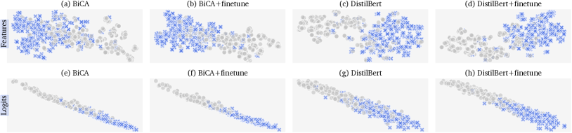
Figure 4: Effects of fine-tuning on BiCA and DistilBert for ACD, where the reference instance is single-aspect. For a fair comparison, all models only have one linear output layer. In the top row, we depict PCA plots of the features before the output layer. The feature dimension in BiCA is 500 and which in DistilBert is 768. In the bottom row, we directly plot the 2-dimensional logits output.

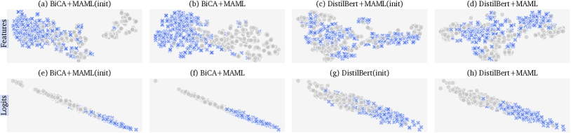
Figure 5: Effects of MAML on BiCA and DistilBert for ACD, where the reference instance is single-aspect. “(init)” indicates that the model learned by MAML training directly predicts the query set of testing meta-tasks without exploiting the support set.

4.4.1 Comparison of Features

We compare the effects of MAML with simple fine-tuning in Figure 4 and Figure 5, respectively. In Figure 4, it can be seen that fine-tuning can help the features learned by BiCA and DistilBert both become more separable (plot a-d). This is also reflected by the 2-dimensional logits output (e-g).

In Figure 5, it can be observed that in MAML training, exploiting the support set can also make the features more discriminative in BiCA (a-b), and so does the logits output (e-f). The features (plot b in Figure 4 and plot b in Figure 5) validates that MAML is more effective than fine-tuning in BiCA.

Model	ACD		HuffPost
	Single	Multi
BiCA	1.74e-3	1.23e-3	2.66e-4
BiCA+finetune	1.77e-3	1.22e-3	2.84e-4
BiCA+MAML(init)	1.79e-3	1.67e-3	3.53e-4
BiCA+MAML	1.92e-3	2.09e-3	5.85e-4
DistilBert	3.35e-3	2.70e-3	1.51e-3
DistilBert+finetune	4.01e-3	3.39e-3	1.78e-3
DistilBert+MAML(init)	8.57e-3	1.15e-2	7.40e-3
DistilBert+MAML	8.98e-3	1.32e-2	7.76e-3
BERT	3.89e-3	3.91e-3	4.62e-3
BERT+finetune	4.83e-3	5.56e-3	6.43e-3
BERT+MAML(init)	2.14e-1	1.71e-1	2.63e-1
BERT+MAML	2.21e-1	1.99e-1	2.58e-1

Table 3: $Cov\_Score$ of various models. The largest is marked in bold for each sequence match model.

Interestingly, the phenomenon of DistilBert+MAML is completely different. It is found that the features show less separability (c-d), while the logits output is well distinguished (g-h). This indicates the features are linearly separable in high dimensions, i.e. 768. Recalling the purpose of PCA (Principal Component Analysis) Abdi and Williams (2010), it defines an orthogonal linear transformation that transforms the data into a new coordinate system and preserves the greatest variance. We guess that the unique phenomena (c-d) are caused by less-orthogonal feature dimensions. To verify this assumption, we compute the covariance matrix based on extracted features in various models. Each element in the matrix indicates the correlation between two dimensions in feature, where a larger score means a higher correlation. We define the $Cov\_Score$ as below, which is the average absolute value of the covariance matrix.

$$Cov\_Score=\mathrm{avg}|\mathrm{Cov}(\mathbf{F}-\mathrm{rowavg}(\mathbf{F}))|$$ (8)

where $\mathbf{F}$ is the extracted features.

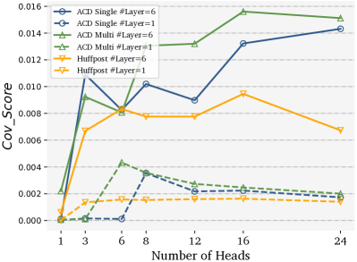
Figure 6: $Cov\_Score$ of the features learned by DistilBert+MAML, setting different numbers of layers, and numbers of heads in self-attention.

In Table 3, the $Cov\_Score$ of three sequence match approaches are presented separately. Firstly, compared with BiCA+finetune, BiCA+MAML extracts features with slightly higher $Cov\_Score$. However, for DistilBert and BERT, MAML dramatically increases the score, which is more significant in BERT. As the scores indicate, DistilBert+MAML really extracts features with less-orthogonal dimensions. A possible reason is that MAML trains the model in a bi-level manner (see Algorithm 1). DistilBert has deeper layers and large-scale parameters. The gradients are propagated through deeper layers, causing the feature extraction learned insufficiently while the last linear layer is trained adequately. Thus the logits are separable while features are not, as plots (c, d, g, h) shown in Figure 5. The above phenomenon become also serious in BERT+MAML, because BERT has more layers compared with DistilBert, leading to larger $Cov\_Score$.

The plots of other datasets are displayed in the Appendix. The empirical observations are similar.

4.4.2 DistilBert+MAML: Layers and Heads?

To further investigate why the features learned by DistilBert+MAML have high-correlation dimensions, we plot the $Cov\_Score$ of multiple variants of DistilBert+MAML in Figure 6. The horizontal ordinate indicates the number of heads in self-attention, which should divide 768 exactly (768 is the dimension size of the hidden states in DistilBert and BERT models).

It is first seen that the score shows an increasing trend as the number of heads grows. Meanwhile, by comparing the curves between #Layer=1 and #Layer=6, we observe that the $Cov\_Score$ also becomes larger as the layers of DistilBert increase. We draw an empirical conclusion that the high-correlation of feature dimensions in DistilBert+MAML is caused by the multiple layers and heads of DistilBert.

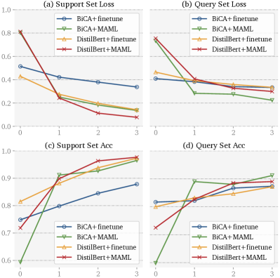
Figure 7: Loss and accuracy curves in 3 updating steps.

4.4.3 Initialization for Loss Sensitivity or a Good Performance Start

In Figure 7, we depict the average batch loss and accuracy in the 3 update steps for ACD with single-aspect references. Step 0 indicates the model is trained by naive training or MAML without using the testing support set.

Concretely, it can be seen that for both BiCA and DistilBert, MAML leads to faster loss degradation than fine-tuning (plot a). The loss in MAML declines to the bottom even within one updating step. We also observe a rapid accuracy increase (c). Overall, MAML outperforms fine-tuning for both BiCA and DistilBert. However, is MAML always a good choice? The answer is negative. In step 0 (b and d), we see a good parameter initialization does not lead to a good performance start. BiCA and DistilBert learned by naive training achieve lower losses and better accuracy scores without updating parameters. A possible explanation is that they have different training objectives. Naive training aims to facilitate task-agnostic sequence matching. While the bi-level optimization in MAML focuses on promoting the generalization ability of models after seeing a few support examples.

4.4.4 Various Numbers of Support Instances

We further explore the performances of BiCA+MAML and DistilBert+MAML under various support set scales. As displayed in Figure 8, the number of support instances ranges from 1 to 10. For a fair comparison, the number of query instances is all set to 10. Firstly, it can be seen that as the support set scale grows, the performances on the query set present an increasing trend. Secondly, we also observe that BiCA+MAML outperforms DistilBert+MAML in most experimental settings. This indicates that classical sequence match is a competitive few-shot one-class learner.

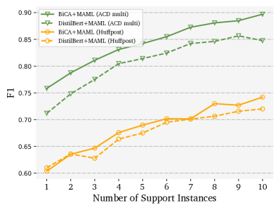
Figure 8: F1 scores of BiCA+MAML and DistilBert+MAML by setting different numbers of support instances.

5 Conclusion

In this work, we revisit the classical sequence match approaches and find that with meta-learning, the classical method can significantly outperform transformer models in the few-shot one-class scenario. The training cost is greatly reduced. Furthermore, an empirical study is made to explore the effects of simple fine-tuning and meta-learning. Interestingly, although meta-learning is more effective than simple fine-tuning on both sequence match approaches, it makes the transformer features have high correlation dimensions. The correlation is closely related to the number of layers and heads in the transformer models. We hope this work could provide insights for future research on few-shot problems and transformer models.

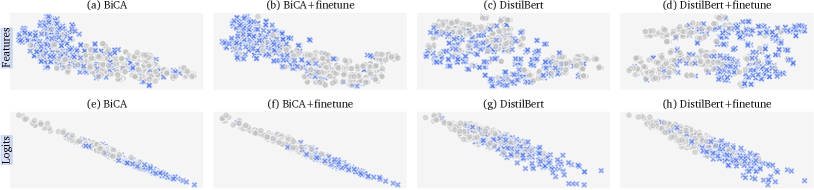
Figure 9: Effects of fine-tuning on aspect category detection, where the reference instance is multi-aspect.

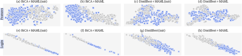
Figure 10: Effects of MAML on aspect category detection, where the reference instance is multi-aspect.

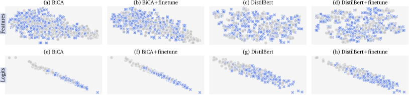
Figure 11: Effects of fine-tuning on HuffPost.

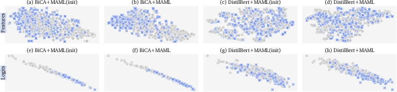
Figure 12: Effects of MAML on HuffPost.

Appendix A Additional Experimental Results

The visualizations of aspect category detection with multi-aspect reference instance are displayed in Figure 9 and Figure 10.

For HuffPost dataset, the visualizations are displayed in Figure 11 and 12.

Appendix B Reproducibility

B.1 Computing Infrastructure

All experiments are conducted on the same hardware and software. We use a single NVIDIA A6000 GPU with 48GB of RAM.

B.2 Average Running time

The average running time of each model is shown in Table 5.

B.3 Number of Parameters

The number of parameters of each model is shown in Table 4.

B.4 Datasets

The datasets are available at https://github.com/hmt2014/FewOne.

B.5 Implementation Details

B.5.1 Classical Methods

All baselines and our model are implemented by Pytorch. We initialize word embeddings with 50-dimension GloVE vectors Pennington et al. (2014). In the aggregation module, the channels of the CNNs for input and output are both 50. The kernel sizes of five CNNs are [1, 2, 3, 4, 5], respectively. $\mathrm{Relu}$ is the activation function for CNN. We adopt a dropout of 0.1 after both the comparison and CNN in aggregation. $\mathrm{MLP}$ is a single linear layer.

The batch size is $|\mathcal{C}_{p}|=5$, indicating a batch comprises 5 meta-tasks. The instance number in the support set $|S|$ and query set $|Q|$ are both set to 10. Every epoch we randomly sample 400 batches for training, 300 batches for validation and 300 batches for testing. The average results of the testing batches are reported. We exploit an early stop strategy during training if the macro-f1 score on the validation set does not improve in 3 epochs, and the best model is chosen for evaluation.

We describe the training details as the format of (optimizer, learning rate, other information):

Naive Training: Adam, 1e-3, early stop.

+finetune   SGD, 0.1, 3 updating steps.

+MAML

The inner-level: $\alpha$=0.1.

The outer-level: Adam, $\beta$=1e-3.

When testing: SGD, 0.1, 3 updating steps.

B.5.2 Transformer-based Methods

The output hidden state of $\mathtt{[CLS]}$ in DistilBert (distilbert-base-uncased) and BERT (bert-base-uncased) is exploited for classification.

Naive Training   Adam, 2e-5, 5 epochs.

+finetune   Adam, 2e-5, 3 updating steps.

+MAML

The inner level: $\alpha$=2e-3.

The outer-level: Adam, $\beta$=2e-5.

When testing: Adam, 2e-5, 3 updating steps.

We use early stop for DistilBert+MAML since the model does not learn optimally within 5 epochs.

Method	ACD	Huffpost
SN	1,437,950	1,393,050
OWP	1,437,950	1,393,050
CA	1,476,202	1,431,302
BiCA	1,476,702	1,431,802
+finetune
+MAML
DistilBert	66,364,418	66,364,418
+finetune
+MAML
BERT	109,483,778	109,483,778
+finetune
+MAML
BERT(p)	133,545,786	133,545,786
+finetune

Table 4: Number of parameters in each model.

Method	ACD		Huffpost
	single	multi
SN	6m47s	11m44s	20m5s
OWP	13m57s	17m49s	11m45s
CA	21m36s	35m17s	18m2s
BiCA	22m26s	18m5s	11m11s
+finetune	20s	20s	23s
BiCA+MAML	39m8s	1h11m57s	40m53s
DistilBert	21m2s	21m26s	21m56s
+finetune	4m45s	4m43s	4m45s
DistilBert+MAML	4h32m2s	4h3m38s	4h46m4s
BERT	39m33s	40m18s	41m27s
+finetune	8m40s	8m41s	9m14s

Table 5: Average runing time of each model.

References

- Abdi and Williams (2010) Hervé Abdi and Lynne J Williams. 2010. Principal component analysis. Wiley interdisciplinary reviews: computational statistics, 2(4):433–459.
- Bao et al. (2020) Yujia Bao, Menghua Wu, Shiyu Chang, and Regina Barzilay. 2020. Few-shot text classification with distributional signatures. In International Conference on Learning Representations (ICLR), pages 1–24.
- Bauman et al. (2017) Konstantin Bauman, Bing Liu, and Alexander Tuzhilin. 2017. Aspect based recommendations: Recommending items with the most valuable aspects based on user reviews. In Proceedings of the 23rd ACM SIGKDD International Conference on Knowledge Discovery and Data Mining (KDD), page 717–725.
- Bian et al. (2017) Weijie Bian, Si Li, Zhao Yang, Guang Chen, and Zhiqing Lin. 2017. A compare-aggregate model with dynamic-clip attention for answer selection. In Proceedings of the 2017 ACM on Conference on Information and Knowledge Management (CIKM), pages 1987–1990.
- Bowman et al. (2015) Samuel Bowman, Gabor Angeli, Christopher Potts, and Christopher D Manning. 2015. A large annotated corpus for learning natural language inference. In Proceedings of the 2015 Conference on Empirical Methods in Natural Language Processing (EMNLP), pages 632–642.
- Devlin et al. (2019) Jacob Devlin, Ming-Wei Chang, Kenton Lee, and Kristina Toutanova. 2019. BERT: Pre-training of deep bidirectional transformers for language understanding. In Proceedings of the 2019 Conference of the North American Chapter of the Association for Computational Linguistics: Human Language Technologies (NAACL), pages 4171–4186.
- Fei-Fei et al. (2006) Li Fei-Fei, Rob Fergus, and Pietro Perona. 2006. One-shot learning of object categories. IEEE transactions on pattern analysis and machine intelligence (TPAMI), 28(4):594–611.
- Feng et al. (2015) Minwei Feng, Bing Xiang, Michael R Glass, Lidan Wang, and Bowen Zhou. 2015. Applying deep learning to answer selection: A study and an open task. In 2015 IEEE Workshop on Automatic Speech Recognition and Understanding (ASRU), pages 813–820.
- Finn et al. (2017) Chelsea Finn, Pieter Abbeel, and Sergey Levine. 2017. Model-agnostic meta-learning for fast adaptation of deep networks. In International conference on machine learning (ICML), pages 1126–1135.
- Frikha et al. (2021) Ahmed Frikha, Denis Krompaß, Hans-Georg Koepken, and Volker Tresp. 2021. Few-shot one-class classification via meta-learning. In The 35th AAAI conference on Artificial Intelligence (AAAI).
- Gao et al. (2021) Tianyu Gao, Adam Fisch, and Danqi Chen. 2021. Making pre-trained language models better few-shot learners. In Proceedings of the 59th Annual Meeting of the Association for Computational Linguistics and the 11th International Joint Conference on Natural Language Processing (ACL-IJCNLP), pages 3816–3830.
- Garcia and Bruna (2018) Victor Garcia and Joan Bruna. 2018. Few-shot learning with graph neural networks. In International Conference on Learning Representations (ICLR).
- Gururangan et al. (2020) Suchin Gururangan, Ana Marasović, Swabha Swayamdipta, Kyle Lo, Iz Beltagy, Doug Downey, and Noah A. Smith. 2020. Don’t stop pretraining: Adapt language models to domains and tasks. In Proceedings of the 58th Annual Meeting of the Association for Computational Linguistics (ACL), pages 8342–8360.
- Kim (2014) Yoon Kim. 2014. Convolutional neural networks for sentence classification. In Proceedings of the 2014 Conference on Empirical Methods in Natural Language Processing (EMNLP), pages 1746–1751.
- Koch et al. (2015) Gregory Koch, Richard Zemel, and Ruslan Salakhutdinov. 2015. Siamese neural networks for one-shot image recognition. In ICML deep learning workshop, pages 1–8.
- Kozerawski and Turk (2018) Jedrzej Kozerawski and Matthew Turk. 2018. Clear: Cumulative learning for one-shot one-class image recognition. In Proceedings of the IEEE Conference on Computer Vision and Pattern Recognition (CVPR), pages 3446–3455.
- Kraus and Feuerriegel (2019) Mathias Kraus and Stefan Feuerriegel. 2019. Personalized purchase prediction of market baskets with wasserstein-based sequence matching. In Proceedings of the 25th ACM SIGKDD International Conference on Knowledge Discovery & Data Mining (KDD), pages 2643–2652.
- Kruspe (2019) Anna Kruspe. 2019. One-way prototypical networks. arXiv preprint arXiv:1906.00820.
- Li et al. (2020) Kai Li, Yulun Zhang, Kunpeng Li, and Yun Fu. 2020. Adversarial feature hallucination networks for few-shot learning. In Proceedings of the IEEE/CVF Conference on Computer Vision and Pattern Recognition (CVPR), pages 13470–13479.
- Li et al. (2019) Zheng Li, Ying Wei, Yu Zhang, Xiang Zhang, and Xin Li. 2019. Exploiting coarse-to-fine task transfer for aspect-level sentiment classification. In Proceedings of the AAAI Conference on Artificial Intelligence (AAAI), volume 33, pages 4253–4260.
- Maaten and Hinton (2008) Laurens van der Maaten and Geoffrey Hinton. 2008. Visualizing data using t-sne. Journal of machine learning research, 9(Nov):2579–2605.
- Misra (2018) Rishabh Misra. 2018. News category dataset.
- Misra and Grover (2021) Rishabh Misra and Jigyasa Grover. 2021. Sculpting Data for ML: The first act of Machine Learning.
- Munkhdalai and Yu (2017) Tsendsuren Munkhdalai and Hong Yu. 2017. Meta networks. In International Conference on Machine Learning (ICML), pages 2554–2563.
- Pennington et al. (2014) Jeffrey Pennington, Richard Socher, and Christopher Manning. 2014. Glove: Global vectors for word representation. In Proceedings of the 2014 Conference on Empirical Methods in Natural Language Processing (EMNLP), pages 1532–1543.
- Rocktäschel et al. (2016) Tim Rocktäschel, Edward Grefenstette, Karl Moritz Hermann, Tomáš Kočiskỳ, and Phil Blunsom. 2016. Reasoning about entailment with neural attention. In International Conference on Learning Representations (ICLR), pages 1–9.
- Sanh et al. (2019) Victor Sanh, Lysandre Debut, Julien Chaumond, and Thomas Wolf. 2019. Distilbert, a distilled version of bert: smaller, faster, cheaper and lighter. The 5th Workshop on Energy Efficient Machine Learning and Cognitive Computing - NeurIPS, pages 1–5.
- Snell et al. (2017) Jake Snell, Kevin Swersky, and Richard Zemel. 2017. Prototypical networks for few-shot learning. In Advances in Neural Information Processing Systems (NeurIPS), pages 4077–4087.
- Song et al. (2020) Yiping Song, Zequn Liu, Wei Bi, Rui Yan, and Ming Zhang. 2020. Learning to customize model structures for few-shot dialogue generation tasks. In Proceedings of the 58th Annual Meeting of the Association for Computational Linguistics (ACL), pages 5832–5841.
- Sung et al. (2018) Flood Sung, Yongxin Yang, Li Zhang, Tao Xiang, Philip HS Torr, and Timothy M Hospedales. 2018. Learning to compare: Relation network for few-shot learning. In Proceedings of the IEEE conference on Computer Vision and Pattern Recognition (CVPR), pages 1199–1208.
- Tapaswi et al. (2016) Makarand Tapaswi, Yukun Zhu, Rainer Stiefelhagen, Antonio Torralba, Raquel Urtasun, and Sanja Fidler. 2016. Movieqa: Understanding stories in movies through question-answering. In Proceedings of the IEEE conference on Computer Vision and Pattern Recognition (CVPR), pages 4631–4640.
- Vaswani et al. (2017) Ashish Vaswani, Noam Shazeer, Niki Parmar, Jakob Uszkoreit, Llion Jones, Aidan N Gomez, Lukasz Kaiser, and Illia Polosukhin. 2017. Attention is all you need. In Advances in Neural Information Processing Systems (NeurIPS).
- Vinyals et al. (2016) Oriol Vinyals, Charles Blundell, Timothy Lillicrap, Daan Wierstra, et al. 2016. Matching networks for one shot learning. In Advances in Neural Information Processing Systems (NeurIPS), pages 3630–3638.
- Wang and Jiang (2017) Shuohang Wang and Jing Jiang. 2017. A compare-aggregate model for matching text sequences. In International Conference on Learning Representations (ICLR).
- Wang et al. (2020) Shuohang Wang, Yunshi Lan, Yi Tay, Jing Jiang, and Jingjing Liu. 2020. Multi-level head-wise match and aggregation in transformer for textual sequence matching. In Proceedings of the AAAI Conference on Artificial Intelligence (AAAI), pages 9209–9216.
- Wang et al. (2018) Yu-Xiong Wang, Ross Girshick, Martial Hebert, and Bharath Hariharan. 2018. Low-shot learning from imaginary data. In Proceedings of the IEEE conference on Computer Vision and Pattern Recognition (CVPR), pages 7278–7286.
- Wright and Augenstein (2020) Dustin Wright and Isabelle Augenstein. 2020. Transformer based multi-source domain adaptation. In (EMNLP), pages 7963–7974.
- Ye and Ling (2019) Zhi-Xiu Ye and Zhen-Hua Ling. 2019. Multi-level matching and aggregation network for few-shot relation classification. In Proceedings of the 57th Annual Meeting of the Association for Computational Linguistics (ACL), pages 2872–2881.
- Yoon et al. (2019) Seunghyun Yoon, Franck Dernoncourt, Doo Soon Kim, Trung Bui, and Kyomin Jung. 2019. A compare-aggregate model with latent clustering for answer selection. In Proceedings of the 28th ACM International Conference on Information and Knowledge Management (CIKM), pages 2093–2096.