Magnetostatic interaction energy between a point magnet and a ring magnet

Abstract

We find an exact closed-form expression for the magnetostatic interaction energy between a point magnet and a ring magnet in terms of complete elliptic integrals. The exact expression for the energy exhibits an equilibrium point close to the axis of symmetry of the ring magnet. Our methodology will be useful in investigations concerning magnetic levitation, and in the study of Casimir levitation.

I Introduction

Configurations with cylindrical symmetry often admit relatively simple solutions on the axis of symmetry, even when the general solution off the axis is given in terms of special functions or has no exact solution. A classic example is that of the magnetic field due to a circular wire carrying a uniform current, where the expression for the magnetic field on the axis is given in terms of rational functions and is usually derived in an introductory level physics course Schwinger et al. (1998), while the solution off the axis is given in terms of complete elliptic integrals and is typically only introduced in a graduate level course Schwinger et al. (1998).

We show that the magnetostatic interaction energy between a point magnet and a ring magnet also admits exact solutions in terms of complete elliptic integrals when the point magnet is off the axis of symmetry of the ring magnet and has a simple solution in terms of rational functions when the point dipole is on the axis of the ring magnet. The interaction energy in general exhibits an equilibrium point close to the axis of symmetry with a saddle point instability. The expression for energy presented here seems to have not been, to our surprise, reported before. However, the corresponding expression for the magnetic field has been discussed in the literature recently Ravaud et al. (2008); Babic and Akyel (2008). The magnetic dipoles in their work are constructed by assuming the existence of magnetic monopoles, which in the static case being considered allows the use of the methodologies developed in electrostatics. The methodology presented here is a useful academic exercise, even though it presumes infinitely thin magnets.

We put forward two applications of the investigation presented here. First is in the study of Casimir levitation. The Casimir effect involves interactions between materials with no net electric charge and no permanent polarizations mediated by the electric and magnetic fields induced from the quantum vacuum fluctuations. Even though repulsion between anisotropically polarizable atoms were well known Axilrod and Teller (1943); Muto (1943); Craig and Power (1969a, b); Babb (2005), perfectly conducting nanoparticles were not expected to show repulsion from interactions with the quantum electromagnetic vacuum fluctuations. Thus, it was a surprise when in Ref. Levin et al. (2010) it was shown that the interaction between an anisotropically shaped conducting nanoparticle and a perfectly conducting metal sheet with a circular aperture could lead to repulsion. Even though an analytic derivation of the result in Ref. Levin et al. (2010) remains unsolved Milton et al. (2011, 2012a); Shajesh et al. (2017), a partial understanding of the repulsion has been made plausible by deriving analogous results in the non-retarded van der Waals regime Eberlein and Zietal (2011) and in the retarded Casimir-Polder regime Milton et al. (2012b); Shajesh and Schaden (2012); Abrantes et al. (2018); Marchetta et al. (2021, 2020). A drawback of all of the above investigations has been the confinement of the nanoparticle to the axis of symmetry in the configuration. Even though it is clear that the nanoparticle is unstable in the transverse directions to the axis in the above considerations, the limitation of being on the axis practically does not allow any stability analysis. Before we embark on evaluating the Casimir-Polder interaction energy between an anisotropically polarizable nanoparticle and an anisotropically polarizable circular ring without restricting the nanoparticle to being on the axis, we here explore the analogous configuration of a permanent magnetic dipole moment interacting with a circular ring with permanent polarization. The methodology we use here can be immediately used to study the corresponding Casimir interaction, which will be presented elsewhere.

The second application is in the study of the magnetic levitation of a Levitron${}^{\text{TM}}$ Berry (1996). In particular, we would like to investigate if the stability of the Levitron${}^{\text{TM}}$ requires the presence of gravity. That is, can a spinning point magnet be stabilized above a ring magnet in the absence of gravity? The interaction energy presented here serves as the starting point for this stability analysis.

In the next section we describe our configuration of a point magnet and a ring magnet and derive the expression for the interaction energy as an integral over the azimuth angle. In Section III we give a brief description of complete elliptic integrals. After introducing complete elliptic integral of the first kind $K(k)$ and second kind $E(k)$ we define elliptic integrals $\pi_{3}(k)$ and $\pi_{5}(k)$, which is not the traditional approach. It should be possible to express the elliptic integrals $\pi_{3}(k)$ and $\pi_{5}(k)$ in terms of the traditional elliptic integral of the third kind. In Section IV we derive the expression for the interaction energy between a point magnet and a ring magnet in terms of the elliptic integrals introduced in Section III. In the final section we present our outlook concerning the investigation of Casimir levitation.

II Magnetostatic energy

Magnetostatics is governed by the Maxwell equations stating that the magnetic field ${\bf B}({\bf r})$ is divergence free,

$${\bm{\nabla}}\cdot{\bf B}=0,$$ (1)

and that current densities ${\bf j}({\bf r})$ are sources for the curl of the magnetic field,

$${\bm{\nabla}}\times{\bf B}=\mu_{0}{\bf j}.$$ (2)

The conservation of charge in the static scenario requires the current densities to be divergence free,

$${\bm{\nabla}}\cdot{\bf j}=0.$$ (3)

The constraint of a divergenceless magnetic field in Eq. (1) allows the construction

$${\bf B}={\bm{\nabla}}\times{\bf A}$$ (4)

in terms of the magnetic vector potential ${\bf A}({\bf r})$. In conjunction with the Coulomb gauge,

$${\bm{\nabla}}\cdot{\bf A}=0,$$ (5)

this allows the solution for the vector potential

$${\bf A}({\bf r})=\frac{\mu_{0}}{4\pi}\int d^{3}r^{\prime}\frac{{\bf j}({\bf r}^{\prime})}{|{\bf r}-{\bf r}^{\prime}|}.$$ (6)

The magnetic dipole moment of a given current density is defined using the expression

$${\bf m}=\frac{1}{2}\int d^{3}r^{\prime}{\bf r}^{\prime}\times{\bf j}({\bf r}^{\prime}).$$ (7)

For a circular current carrying loop of wire we have $m=IA$, where $I$ is the current in the wire and $A$ is the area of the circular loop. A point magnetic dipole is an idealized construction with $I\to\infty$ and $A\to 0$, keeping the product $m=IA$ fixed. We shall be interested in the interaction between a point magnetic dipole ${\bf m}_{1}$ and a ring magnet constructed out of a uniform circular distribution of point dipoles ${\bf m}_{2}$.

The magnetic vector potential at position ${\bf r}$ due to a point magnetic dipole moment ${\bf m}_{2}$ placed at position ${\bf r}^{\prime}$ is

$${\bf A}_{2}({\bf R})=\frac{\mu_{0}}{4\pi}\frac{{\bf m}_{2}\times{\bf R}}{R^{3}},$$ (8)

where

$${\bf R}={\bf r}-{\bf r}^{\prime}.$$ (9)

The associated magnetic field due to the point magnet is obtained using

$${\bf B}_{2}={\bm{\nabla}}\times{\bf A}_{2}$$ (10)

and leads to the expression

$${\bf B}_{2}({\bf R})=\frac{\mu_{0}}{4\pi}\frac{\big{[}3\hat{\bf R}\hat{\bf R}-{\bf 1}\big{]}\cdot{\bf m}_{2}}{R^{3}},\qquad{\bf r}\neq{\bf r}^{\prime},$$ (11)

where $\hat{\bf R}={\bf R}/R$. This expression for the magnetic field in Eq. (11) is missing a term $\mu_{0}{\bf m}_{2}\delta^{(3)}({\bf r}-{\bf r}^{\prime})$ which contributes only at ${\bf r}={\bf r}^{\prime}$ and is necessary to satisfy the constraint

$${\bm{\nabla}}\cdot{\bf B}_{2}=0.$$ (12)

The magnetostatic interaction energy between another point magnetic dipole ${\bf m}_{1}$ and the dipole ${\bf m}_{2}$ is given by

$$U({\bf r})=-{\bf m}_{1}\cdot{\bf B}_{2}({\bf r}),$$ (13)

where ${\bf r}$ now is the position of the point magnet ${\bf m}_{1}$.

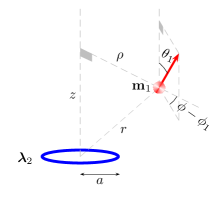
Figure 1: A point magnet of magnetic dipole moment ${\bf m}_{1}=m_{1}\hat{\bf n}$ at height $z$ above a ring magnet of radius $a$ with uniform magnetic dipole moment per unit length ${\bm{\lambda}}_{2}$. The point magnet is a distance $\rho$ away from the axis of symmetry of the ring magnet. The dipole moment subtends an angle $\theta_{1}$ with respect to the axis of symmetry, that is, $\hat{\bf n}\cdot\hat{\bf z}=\cos\theta_{1}$.

A ring magnet is described by its magnetic moment per unit length

$${\bm{\lambda}}_{2}=\frac{d{\bf m}_{2}}{ad\phi},$$ (14)

where $a$ is the radius of the ring and $ad\phi$ is the differential arc length. Let us choose the magnetic moment of the ring to be uniform and along the axis of symmetry of the ring, say $\hat{\bf z}$, such that

$${\bm{\lambda}}_{2}=\lambda_{2}\hat{\bf z}.$$ (15)

We further choose the ring to be in the $z=0$ plane centered at the origin. Refer Fig. 1. Let us keep the orientation of the point magnet arbitrary relative to the ring magnet and describe it as

$${\bf m}_{1}=m_{1}\hat{\bf n},$$ (16)

where

$$\hat{\bf n}=\sin\theta_{1}\cos\phi_{1}\hat{\bf x}+\sin\theta_{1}\sin\phi_{1}\hat{\bf y}+\cos\theta_{1}\hat{\bf z},$$ (17)

such that

$$\hat{\bf n}\cdot\hat{\bf z}=\cos\theta_{1}$$ (18)

with its position

$${\bf r}=\rho\cos\phi\hat{\bf x}+\rho\sin\phi\hat{\bf y}+z\hat{\bf z}.$$ (19)

Note that

$$\hat{\bf n}\cdot{\bf r}=\rho\sin\theta_{1}\cos(\phi-\phi_{1}),$$ (20)

which illustrates that the vectors ${\bf m}_{1}$ and ${\bm{\lambda}}_{2}$ representing the orientation of the dipoles and ${\bf r}$ are not in the same plane.

Differential contribution to the interaction energy from the interaction between the point magnet and a differential section of the ring magnet is given by

$$dU=-{\bf m}_{1}\cdot d{\bf B}_{2},$$ (21)

where using Eq. (11)

$$d{\bf B}_{2}({\bf R})=\frac{\mu_{0}}{4\pi}\frac{\big{[}3\hat{\bf R}\hat{\bf R}-{\bf 1}\big{]}\cdot d{\bf m}_{2}}{R^{3}}$$ (22)

with ${\bf r}^{\prime}$ now constrained to be on the ring by $z^{\prime}=0$ and $|{\bf r}^{\prime}|=a$ such that

$${\bf r}^{\prime}=a\cos\phi^{\prime}\hat{\bf x}+a\sin\phi^{\prime}\hat{\bf y}+0\hat{\bf z}.$$ (23)

Using Eq. (14) the differential interaction energy takes the form

$$dU=\frac{\mu_{0}}{4\pi}\frac{{\bf m}_{1}\cdot\big{[}{\bf 1}-3\hat{\bf R}\hat{\bf R}\big{]}\cdot{\bm{\lambda}}_{2}}{R^{3}}ad\phi^{\prime}$$ (24)

from which the total interaction energy can be calculated by integrating over angle $\phi^{\prime}$ and is given by

$$U=\frac{\mu_{0}}{4\pi}m_{1}\lambda_{2}\int_{0}^{2\pi}ad\phi^{\prime}\left[\frac{(\hat{\bf n}\cdot\hat{\bf z})}{R^{3}}-\frac{(\hat{\bf n}\cdot{\bf R})({\bf R}\cdot\hat{\bf z}}{R^{5}}\right],$$ (25)

where

$$R=\sqrt{z^{2}+a^{2}+\rho^{2}-2a\rho\cos(\phi^{\prime}-\phi)}.$$ (26)

We have $(\hat{\bf n}\cdot\hat{\bf z}$) using Eq. (18),

$${\bf R}\cdot\hat{\bf z}=z,$$ (27)

and

$$\hat{\bf n}\cdot{\bf R}=\rho\sin\theta_{1}\cos(\phi-\phi_{1})-a\sin\theta_{1}\cos(\phi^{\prime}-\phi_{1})+z\cos\theta_{1}.$$ (28)

Using these expressions the magnetostatic interaction energy between the point magnet and the ring magnet is given by

$$U(z,\rho,\phi-\phi_{1},\theta_{1})=\frac{\mu_{0}}{4\pi}\frac{m_{1}(2\pi\lambda_{2})}{a^{2}}\int_{0}^{2\pi}\frac{d\phi^{\prime}}{2\pi}$$

$$\times\Bigg{[}\frac{a^{3}\cos\theta_{1}}{R^{3}}-\frac{3a^{3}z^{2}\cos\theta_{1}}{R^{5}}-\frac{3a^{3}z\rho\sin\theta_{1}\cos(\phi-\phi_{1})}{R^{5}}$$

$$\hskip 11.38109pt+\frac{3a^{4}z\sin\theta_{1}\cos(\phi^{\prime}-\phi_{1})}{R^{5}}\Bigg{]}.\hskip 22.76219pt$$ (29)

In the special circumstance when the point magnet is positioned on the axis of the ring we have $\rho=0$. This allows the integrals on $\phi^{\prime}$ in Eq. (29) to be completed and yields an exact expression for the interaction energy for this scenario as

$$U(z,0,\phi-\phi_{1},\theta_{1})=\frac{\mu_{0}}{4\pi}\frac{m_{1}(2\pi\lambda_{2})}{a^{2}}\frac{a^{3}(a^{2}-2z^{2})}{(a^{2}+z^{2})^{\frac{5}{2}}}\cos\theta_{1},$$ (30)

which has an extremum at

$$z=h=\pm a\sqrt{\frac{3}{2}}.$$ (31)

When the point magnet is positioned at this extremum point $z=h$ on the axis we have

$$U(h,0,\phi-\phi_{1},\theta_{1})=-\frac{\mu_{0}}{4\pi}\frac{m_{1}(2\pi\lambda_{2})}{a^{2}}\frac{8}{25}\sqrt{\frac{2}{5}}\cos\theta_{1}.$$ (32)

In general, for $\rho\neq 0$, the integrals on $\phi^{\prime}$ can not be completed in terms of elementary functions. However, they can be expressed in terms of complete elliptic integrals. In the following section, we shall evaluate the exact and approximate form for the elliptic integrals required to express Eq. (29) for $\rho\neq 0$ off the axis.

III Complete elliptic integrals

Complete elliptic integrals of the first and second kind can be defined using the integral representations DLMF ; NIS (2010)

$$K(k) = \int_{0}^{\frac{\pi}{2}}d\psi\frac{1}{\sqrt{1-k^{2}\sin^{2}\psi}},$$ (33a)

$$E(k) = \int_{0}^{\frac{\pi}{2}}d\psi\sqrt{1-k^{2}\sin^{2}\psi},$$ (33b)

respectively. We will be interested in the domain $0\leq k<1$. These integrals can not be completed and expressed in terms of elementary functions. However, for special values they can be evaluated easily. For example, we can verify that

$$K(0) = \frac{\pi}{2},$$ (34a)

$$E(0) = \frac{\pi}{2}.$$ (34b)

Further, we can verify that

$$E(1)=1.$$ (35)

Note that

$$K(1)=\int_{0}^{\frac{\pi}{2}}\frac{d\psi}{\cos\psi}$$ (36)

is divergent. To see the nature of this divergence we can introduce a cutoff parameter $\delta>0$ and write

$$K(1)=\lim_{\delta\to 0}\int_{0}^{\frac{\pi}{2}-\delta}\frac{d\psi}{\cos\psi},$$ (37)

which when evaluated using the identity $d(\sec\psi+\tan\psi)=\sec\psi(\sec\psi+\tan\psi)d\psi$ yields

$$K(1)\sim\ln 2-\ln\delta-\frac{\delta^{2}}{12}+{\cal O}(\delta)^{4}$$ (38)

and reveals that $K(1)$ has a logarithmic divergence. The plots of $K(k)$ and $E(k)$ as functions of $k$ for $0\leq k<1$ are shown in Fig. 2. The complete elliptic integrals in Eqs. (33) have the power series expansions

$$K(k) = \frac{\pi}{2}\sum_{n=0}^{\infty}\left[\frac{(2n)!}{2^{2n}(n!)^{2}}\right]^{2}k^{2n}$$ (39a)

$$= \frac{\pi}{2}\left[1+\frac{1}{4}k^{2}+\frac{9}{64}k^{4}+\ldots\right],$$ (39b)

$$E(k) = \frac{\pi}{2}\sum_{n=0}^{\infty}\left[\frac{(2n)!}{2^{2n}(n!)^{2}}\right]^{2}\frac{k^{2n}}{(1-2n)}$$ (39c)

$$= \frac{\pi}{2}\left[1-\frac{1}{4}k^{2}-\frac{3}{64}k^{4}-\ldots\right].$$ (39d)

The leading order contribution in the power series expansions are from $K(0)$ and $E(0)$. The next-to-leading order contributions in the above series expansions are evaluated by expanding the radical in Eqs.(33) as a series using

$$\frac{1}{\sqrt{1-x}} = 1+\frac{1}{2}x+\dots,$$ (40a)

$$\sqrt{1-x} = 1-\frac{1}{2}x+\dots.$$ (40b)

Either the integral representations or the series expansions are sufficient to investigate the properties of the complete elliptic integrals. Here we shall primarily use the integral representations, and depend on the series expansions occasionally.

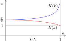
Figure 2: Complete elliptic integrals of the first kind $K(k)$ and of the second kind $E(k)$, plotted as a function of $k$. Both the functions evaluate to $\pi/2$ for $k=0$. For $k\to 1$ the elliptic integral of the second kind approaches 1 and the elliptic integral of the first kind grows logarithmically.

To get some insight for complete elliptic integrals we mention three physical situations where one encounters these functions. Firstly, if we had sought to evaluate the perimeter of an ellipse during our exposure to geometry, we would have encountered the complete elliptic integral of the second kind. The perimeter $C$ of an ellipse, described by the equation

$$\frac{x^{2}}{a^{2}}+\frac{y^{2}}{b^{2}}=1$$ (41)

and characterized by the eccentricity

$$e=\sqrt{1-\frac{b^{2}}{a^{2}}}$$ (42)

in terms of the semi-major axis $a$ and semi-minor axis $b$, is given in terms of complete elliptic integral of the second kind as

$$C=4aE(e).$$ (43)

A circle is an ellipse of zero eccentricity ($a=b$) and has the circumference

$$C\to 4aE(0)=2\pi a$$ (44)

using $E(0)=\pi/2$. Secondly, the period of oscillations $T$ of the simple pendulum as a function of the amplitude of oscillations $\phi_{0}$ is given in terms of the complete elliptic integral of the first kind as

$$T=2\pi\sqrt{\frac{l}{g}}\,\frac{2}{\pi}K\left(\sin\frac{\phi_{0}}{2}\right).$$ (45)

For small amplitudes ($\phi_{0}\ll 1$) this reproduces the classic result

$$T\to 2\pi\sqrt{\frac{l}{g}}\,\frac{2}{\pi}K\left(0\right)=2\pi\sqrt{\frac{l}{g}}$$ (46)

using $K(0)=\pi/2$. Thirdly, one encounters elliptic integrals while finding the magnetic field due to a circular wire carrying a steady current, at points away from the axis of symmetry of the circular wire Schwinger et al. (1998).

Derivatives of the elliptic integrals with respect to their arguments are calculated by evaluating the derivatives of the corresponding integrands and then rewriting the resultant integrals in terms of elliptic integrals. This process is simplified by introducing new elliptic integrals. The derivative of the complete elliptic integral of the second kind leads to the integral

$$\frac{dE}{dk}=-k\int_{0}^{\frac{\pi}{2}}d\psi\frac{\sin^{2}\psi}{\sqrt{1-k^{2}\sin^{2}\psi}},$$ (47)

which can be rewritten in the form

$$\frac{dE}{dk}=\frac{1}{k}\int_{0}^{\frac{\pi}{2}}d\psi\frac{\big{[}-1+1-k^{2}\sin^{2}\psi\big{]}}{\sqrt{1-k^{2}\sin^{2}\psi}}$$ (48)

to recognize the identity

$$\frac{dE}{dk}=-\frac{K(k)}{k}+\frac{E(k)}{k}.$$ (49)

Following the same steps for $K(k)$ yields

$$\frac{dK}{dk}=\frac{\pi_{3}(k)}{k}-\frac{K(k)}{k},$$ (50)

where we introduced a new elliptic integral

$$\pi_{3}(k)=\int_{0}^{\frac{\pi}{2}}d\psi\frac{1}{(1-k^{2}\sin^{2}\psi)^{\frac{3}{2}}}.$$ (51)

The new elliptic integral $\pi_{3}(k)$ can be written in terms of $K(k)$ and $E(k)$. To obtain this result, we rewrite the integral in Eq. (47) in the form

$$\frac{dE}{dk}=k\int_{0}^{\frac{\pi}{2}}d\psi\frac{\sin\psi}{\sqrt{1-k^{2}\sin^{2}\psi}}\frac{d}{d\psi}\cos\psi$$ (52)

and integrate by parts to write

$$\frac{dE}{dk} = k\int_{0}^{\frac{\pi}{2}}d\psi\frac{d}{d\psi}\left[\frac{\sin\psi\cos\psi}{\sqrt{1-k^{2}\sin^{2}\psi}}\right]$$ (53)

$$-k\int_{0}^{\frac{\pi}{2}}d\psi\cos\psi\frac{d}{d\psi}\left[\frac{\sin\psi}{\sqrt{1-k^{2}\sin^{2}\psi}}\right].\hskip 8.53581pt$$

The first integrand is a total derivative and thus contributes only at the boundary, and yields zero in this case at both ends. The second integral, after evaluating the derivative in the integrand, takes the form

$$\frac{dE}{dk}=\int_{0}^{\frac{\pi}{2}}d\psi\frac{-k\cos^{2}\psi}{(1-k^{2}\sin^{2}\psi)^{\frac{3}{2}}}.$$ (54)

Rewriting the numerator of the integrand as

$$-k\cos^{2}\phi=\frac{(1-k^{2})}{k}-\frac{(1-k^{2}\sin^{2}\psi)}{k}$$ (55)

allows us to recognize the integrals as

$$\frac{dE}{dk}=\pi_{3}(k)\frac{(1-k^{2})}{k}-\frac{K(k)}{k}.$$ (56)

Thus, we have derived two separate expressions for $dE/dk$ in Eqs. (49) and (56). Equating the right hand sides of these equations allows us to find an identity for $\pi_{3}(k)$ in terms of $E(k)$,

$$\pi_{3}(k)=\frac{E(k)}{(1-k^{2})}.$$ (57)

Using the power series expansion for $E(k)$ together with the power series expansion of $1/(1-k^{2})$ we obtain the power series expansion for $\pi_{3}(k)$ as

$$\pi_{3}(k)=\frac{\pi}{2}\left[1+\frac{3}{4}k^{2}+\frac{45}{64}k^{4}+\ldots\right].$$ (58)

When we follow the steps leading to Eq. (49) for $\pi_{3}(k)$ we obtain

$$\frac{d\pi_{3}}{dk}=\frac{3}{k}\Big{[}\pi_{5}(k)-\pi_{3}(k)\Big{]},$$ (59)

where

$$\pi_{5}(k)=\int_{0}^{\frac{\pi}{2}}d\psi\frac{1}{(1-k^{2}\sin^{2}\psi)^{\frac{5}{2}}}.$$ (60)

Starting from the definition of $K(k)$ we have the derivative

$$\frac{dK}{dk}=k\int_{0}^{\frac{\pi}{2}}d\psi\frac{\sin^{2}\psi}{(1-k^{2}\sin^{2}\psi)^{\frac{3}{2}}}.$$ (61)

Using the identity $\sin^{2}\psi d\psi=-\sin\psi d\cos\psi$, like earlier in Eq. (52), we integrate by parts to obtain

$$\frac{dK}{dk}=\int_{0}^{\frac{\pi}{2}}d\psi\frac{k\cos^{2}\psi(1+2k^{2}\sin^{2}\psi)}{(1-k^{2}\sin^{2}\psi)^{\frac{5}{2}}}.$$ (62)

Again, rewriting the numerator as

$$\cos^{2}\psi(1+2k^{2}\sin^{2}\psi)=-\frac{3(1-k^{2})}{k^{2}}\hskip 79.66771pt$$

$$\hskip 8.53581pt+\frac{(5-2k^{2})}{k^{2}}(1-k^{2}\sin^{2}\psi)-\frac{2}{k^{2}}(1-k^{2}\sin^{2}\psi)^{2}\hskip 14.22636pt$$ (63)

leads to the identity

$$\frac{dK}{dk}=-\frac{3(1-k^{2})}{k^{2}}\pi_{5}(k)+\frac{(5-2k^{2})}{k^{2}}\pi_{3}(k)-\frac{2}{k^{2}}K(k).$$ (64)

Using Eqs. (50) and (64) we have

$$\pi_{5}(k)=\frac{2(2-k^{2})}{3(1-k^{2})}\pi_{3}(k)-\frac{K(k)}{3(1-k^{2})}.$$ (65)

We can further replace $\pi_{3}(k)$ Eq. (57) to write

$$\pi_{5}(k)=\frac{2(2-k^{2})}{3(1-k^{2})^{2}}E(k)-\frac{K(k)}{3(1-k^{2})}.$$ (66)

The power series expansion for $\pi_{5}(k)$ yields

$$\pi_{5}(k)=\frac{\pi}{2}\left[1+\frac{5}{4}k^{2}+\frac{105}{64}k^{4}+\ldots\right].$$ (67)

For the present discussion it is also handy to have the series expansion

$$\left(\pi_{5}(k)-\frac{2}{k^{2}}\Big{\{}\pi_{5}(k)-\pi_{3}(k)\Big{\}}\right)\hskip 85.35826pt$$

$$\hskip 56.9055pt=\frac{\pi}{2}\Big{[}0-\frac{5}{8}k^{2}-\frac{35}{32}k^{4}+\ldots\Big{]}.$$ (68)

IV Magnetostatic energy in terms of complete elliptic integrals

To express the magnetostatic interaction energy in Eq. (29) in terms of elliptic integrals, we start by substituting $\phi^{\prime\prime}=\phi^{\prime}-\phi$, which takes the limit of integrations from $-\phi$ to $2\pi-\phi$. Since the integration is a sum, it does not care for the order as long as it completes a period. Thus, we can switch the limits of integration to go from $-\pi$ to $+\pi$. This leads to

$$U = \frac{\mu_{0}}{4\pi}\frac{m_{1}(2\pi\lambda_{2})}{a^{2}}\int_{-\pi}^{\pi}\frac{d\phi^{\prime\prime}}{2\pi}\Bigg{[}\frac{a^{3}\cos\theta_{1}}{R^{3}}-\frac{3a^{3}z^{2}\cos\theta_{1}}{R^{5}}$$ (69)

$$-\frac{3a^{3}z\rho\sin\theta_{1}\cos(\phi-\phi_{1})}{R^{5}}$$

$$+\frac{3a^{4}z\sin\theta_{1}\cos(\phi^{\prime\prime}+\phi-\phi_{1})}{R^{5}}\Bigg{]},$$

where, now, $R^{2}=z^{2}+a^{2}+\rho^{2}-2a\rho\cos\phi^{\prime\prime}$. The integral associated with the fourth term evaluates partly to zero, after using $\cos(\phi^{\prime\prime}+\phi-\phi_{1})=\cos\phi^{\prime\prime}\cos(\phi-\phi_{1})-\sin\phi^{\prime\prime}\sin(\phi-\phi_{1})$, because the integrand containing $\sin\phi^{\prime\prime}$ is odd, and the rest being even are twice the value when integrating from 0 to $\pi$. Thus,

$$U = \frac{\mu_{0}}{4\pi}\frac{m_{1}(2\pi\lambda_{2})}{a^{2}}\int_{0}^{\pi}\frac{d\phi^{\prime\prime}}{2\pi}\Bigg{[}\frac{2a^{3}\cos\theta_{1}}{R^{3}}-\frac{6a^{3}z^{2}\cos\theta_{1}}{R^{5}}$$ (70)

$$-\frac{6a^{3}z\sin\theta_{1}\cos(\phi-\phi_{1})(\rho-a\cos\phi^{\prime\prime})}{R^{5}}\Bigg{]}.$$

To prepare the denominator for the elliptic integrals we substitute $\phi^{\prime\prime}=\pi-\phi^{\prime}$, which amounts to integrating in the reverse order. This amounts to replacing $\cos\phi^{\prime}\to\cos(\pi-\phi^{\prime})=-\cos\phi^{\prime}$. That is,

$$U = \frac{\mu_{0}}{4\pi}\frac{m_{1}(2\pi\lambda_{2})}{a^{2}}\int_{0}^{\pi}\frac{d\phi^{\prime}}{2\pi}\Bigg{[}\frac{2a^{3}\cos\theta_{1}}{(a^{2}+z^{2}+\rho^{2}+2a\rho\cos\phi^{\prime})^{\frac{3}{2}}}$$ (71)

$$-\frac{6a^{3}z^{2}\cos\theta_{1}}{(a^{2}+z^{2}+\rho^{2}+2a\rho\cos\phi^{\prime})^{\frac{5}{2}}}$$

$$-\frac{6a^{3}z\sin\theta_{1}\cos(\phi-\phi_{1})(\rho+a\cos\phi^{\prime})}{(a^{2}+z^{2}+\rho^{2}+2a\rho\cos\phi^{\prime})^{\frac{5}{2}}}\Bigg{]}.$$

Using the trigonometric identity $\cos\phi^{\prime}=1-2\sin^{2}(\phi^{\prime}/2)$ and substituting $\phi^{\prime}/2\to\phi^{\prime}$ afterwards, we obtain

$$U = \frac{\mu_{0}}{4\pi}\frac{m_{1}(2\pi\lambda_{2})}{a^{2}}\sqrt{\frac{a}{\rho}}\int_{0}^{\frac{\pi}{2}}\frac{d\psi}{2\pi}\Bigg{[}\frac{ak^{3}\cos\theta_{1}}{2\rho(1-k^{2}\sin^{2}\psi)^{\frac{3}{2}}}$$ (72)

$$-\frac{3z^{2}k^{5}\cos\theta_{1}}{8\rho^{2}(1-k^{2}\sin^{2}\psi)^{\frac{5}{2}}}-\frac{3zak^{5}\sin\theta_{1}\cos(\phi-\phi_{1})}{8\rho^{2}(1-k^{2}\sin^{2}\psi)^{\frac{5}{2}}}$$

$$\times\left\{\frac{\rho}{a}+(1-2\sin^{2}\psi)\right\}\Bigg{]}.$$

We can recognize the elliptic integrals $\pi_{3}(k)$ and $\pi_{5}(k)$ introduced in Eqs. (51) and (60), respectively, in the first two integrals and in the first term of the third integral. The elliptic integrals here are written in terms of the argument $k$ defined using

$$k^{2}=\frac{4a\rho}{z^{2}+(a+\rho)^{2}}.$$ (73)

The second term in the third integral can be expressed in terms of elliptic integrals as

$$\int_{0}^{\frac{\pi}{2}}d\psi\frac{(1-2\sin^{2}\psi)}{(1-k^{2}\sin^{2}\psi)^{\frac{5}{2}}}\hskip 85.35826pt$$

$$\hskip 28.45274pt=\left(\pi_{5}(k)-\frac{2}{k^{2}}\Big{\{}\pi_{5}(k)-\pi_{3}(k)\Big{\}}\right).$$ (74)

Then, in terms of elliptic integrals, we obtain an exact analytic expression for the magnetostatic interaction energy between the point dipole and the ring magnet as

$$U(z,\rho,\phi-\phi_{1},\theta_{1}) = \frac{\mu_{0}}{4\pi}\frac{m_{1}(2\pi\lambda_{2})}{a^{2}}\sqrt{\frac{a}{\rho}}\frac{1}{4}\frac{2}{\pi}\Bigg{[}\frac{1}{2}\frac{a}{\rho}\cos\theta_{1}k^{3}\pi_{3}(k)-\frac{3}{8}\left(\frac{z^{2}}{\rho^{2}}\cos\theta_{1}+\frac{z}{\rho}\sin\theta_{1}\cos(\phi-\phi_{1})\right)k^{5}\pi_{5}(k)$$ (75)

$$\hskip 96.73936pt-\frac{3}{8}\frac{a}{\rho}\frac{z}{\rho}\sin\theta_{1}\cos(\phi-\phi_{1})k^{5}\left(\pi_{5}(k)-\frac{2}{k^{2}}\Big{\{}\pi_{5}(k)-\pi_{3}(k)\Big{\}}\right)\Bigg{]}.$$

The expression for the interaction energy in Eq. (75) is valid for arbitrary position and orientation of the point magnet. We shall proceed to list some special cases of positions and orientations, which are expected to give insight into the structure of the interaction energy.

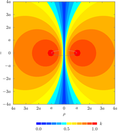
Figure 3: Contour plot of the parameter $k$ defined in Eq. (73) as a function of $\rho$ and $z$. In the figure, $k=0$ corresponds to the $z$ axis where $\rho=0$, and $k=1$ corresponds to the ring described by $\rho=a$. The region corresponding to $k\ll 1$ consists of points very close to the $z$ axis.

In the special case when the point magnet is positioned on the axis of symmetry of the ring magnet we have $\rho=0$, which sets $k=0$. We keep the orientation of the point magnet arbitrary. The parameter $0\leq k<1$ spans the complete region around the ring magnet. $k=1$ corresponding to the ring magnet itself, given by $\rho=a$ and $z=0$, which can not be occupied by the point magnet. The region of space around the ring magnet, as described by the parameter $k$ in terms of $\rho$ and $z$ is illustrated in Fig. 3. Using the leading order contributions in Eqs.(58) and (67),

$$\pi_{3}(k) = \frac{\pi}{2}\Big{[}1+{\cal O}(k^{2})\Big{]},$$ (76a)

$$\pi_{5}(k) = \frac{\pi}{2}\Big{[}1+{\cal O}(k^{2})\Big{]},$$ (76b)

and Eq.(68),

$$\left(\pi_{5}(k)-\frac{2}{k^{2}}\Big{\{}\pi_{5}(k)-\pi_{3}(k)\Big{\}}\right)=\frac{\pi}{2}\Big{[}0+{\cal O}(k^{2})\Big{]},$$ (77)

and $\lim_{\rho\to 0}k^{2}/\rho=4a/(z^{2}+a^{2})$, in Eq. (75), we reproduce the interaction energy in Eq. (30) successfully, for this particular case. This serves as a partial check for the exact expression in Eq. (75).

For the special case when the orientation of the point magnet is parallel to the axis of the ring magnet we have

$$U(z,\rho,\phi-\phi_{1},0)=\frac{\mu_{0}}{4\pi}\frac{m_{1}(2\pi\lambda_{2})}{a^{2}}\left(\frac{a}{\rho}\right)^{\frac{3}{2}}\frac{k^{3}}{8}\hskip 28.45274pt$$

$$\hskip 56.9055pt\times\frac{2}{\pi}\left[\pi_{3}(k)-\frac{3z^{2}k^{2}}{4a\rho}\pi_{5}(k)\right]$$ (78)

for arbitrary position of the point magnet. Observe that it is independent of the variable $\phi$ representing the azimuth angle of the position of the point magnet leading to axial symmetry, in addition to the trivial independence in orientation variable $\phi_{1}$ because of $\theta_{1}=0$. Further, we have

$$U\left(z,\rho,\frac{\pi}{2},\theta_{1}\right)=\cos\theta_{1}\,U(z,\rho,\phi-\phi_{1},0).$$ (79)

The interpretation is that, when the azimuthal plane of position of the point dipole is perpendicular to the azimuthal plane of its orientation, the energy is simply a scaled version of an axially oriented point magnet. As a consequence of Eq. (79) we have the interaction energy to be zero when the orientation of the point magnet is perpendicular to the position vector of the point magnet, $\theta_{1}=\pi/2$. That is,

$$U\left(z,\rho,\frac{\pi}{2},\frac{\pi}{2}\right)=0.$$ (80)

Next, if we have $\theta_{1}=\pi/2$ with arbitrary $\phi-\phi_{1}$ we have

$$U\left(z,\rho,\phi-\phi_{1},\frac{\pi}{2}\right)=\frac{\mu_{0}}{4\pi}\frac{m_{1}(2\pi\lambda_{2})}{a^{2}}\sqrt{\frac{a}{\rho}}\frac{3zk^{5}}{32\rho}\cos(\phi-\phi_{1})$$

$$\times\frac{2}{\pi}\Bigg{[}\pi_{5}(k)+\frac{a}{\rho}\left(\pi_{5}(k)-\frac{2}{k^{2}}\Big{\{}\pi_{5}(k)-\pi_{3}(k)\Big{\}}\right)\Bigg{]}.\hskip 22.76219pt$$ (81)

V Conclusion and outlook

In Eq. (75) we have presented an exact expression for the magnetostatic interaction energy between a point magnet and a ring magnet in terms of complete elliptic integrals. Starting from this energy expression we can analyze the stability of the point magnet. Our configuration is essentially that of a massless point-like Levitron${}^{\text{TM}}$, the stability analysis of which has been discussed in Ref. Berry (1996). However, the investigation in Ref. Berry (1996) is assumed to be on the axis of symmetry. Our expression for energy derived here allows an accurate analytical derivation of the stability. This requires us to find the force on the point dipole, which is given in terms of the derivatives of the elliptic integrals in the energy. However, to find the stability points this would amount to finding the zeros of an expression involving elliptic integrals. This will inevitably force us to depend on numerics. However, since the stability points are expected to be close to the axis we will be able to depend on the series expansions and obtain analytic perturbative expressions. This will be explored in another discussion elsewhere.

Our primary long-term goal is to discuss Casimir levitation, as proposed in and around FIG. 16 of Ref. Marchetta et al. (2020). Here we outline how the methodology presented here can be immediately used to derive the corresponding Casimir-Polder interaction energy between a polarizable atom of polarizability

$${\bm{\alpha}}=\alpha_{1}\hat{\bf n}\hat{\bf n}$$ (82)

and a polarizable ring of radius $a$ with electric susceptibility

$${\bm{\chi}}=\sigma_{2}\hat{\bf z}\hat{\bf z}\delta(z^{\prime}-0)\delta(\rho^{\prime}-a).$$ (83)

Here $\hat{\bf n}$ is the principal axis of polarization and is chosen to be given using Eq. (17). Similarly, $\hat{\bf z}$ is the direction of polarization of the ring. The position of the atom is ${\bf r}$ and chosen to be given using Eq. (19), and a point on the ring is described by ${\bf r}^{\prime}$ given using Eq. (23), Thus, the parameters in the problem are equivalent to those of the magnetic configuration presented in this article. The Casimir-Polder interaction energy between the atom and the ring is given using Eq. (41) in Ref. Marchetta et al. (2020), which can rewritten in terms of the parameters in this article as

$$U = -\frac{\hbar c}{32\pi^{2}}\int d^{3}x\left[13\frac{\text{tr}({\bm{\alpha}}\cdot{\bm{\chi}})}{R^{7}}-56\frac{({\bf R}\cdot{\bm{\alpha}}\cdot{\bm{\chi}}\cdot{\bf R})}{R^{9}}\right.$$ (84)

$$\hskip 62.59605pt\left.+63\frac{({\bf R}\cdot{\bm{\alpha}}\cdot{\bf R})({\bf R}\cdot{\bm{\chi}}\cdot{\bf R})}{R^{11}}\right],$$

where the vector ${\bf R}$ is given by Eq. (9) and the magnitude $R$ is given by Eq. (26). In Ref. Marchetta et al. (2020) the atom was confined on the symmetry axis and it led to the significantly simplified expression for energy in Eq. (103) there. When we do not restrict the atom to be on the axis of symmetry we have the expression for energy

$$U(z,\rho,\phi-\phi_{1},\theta_{1})=-\frac{\hbar c\,\alpha_{1}\sigma_{2}a}{32\pi^{2}}\int_{0}^{2\pi}d\phi^{\prime}\left[13\frac{(\hat{\bf n}\cdot\hat{\bf z})^{2}}{R^{7}}\right.\hskip 2.84526pt$$

$$\left.-56\frac{({\bf R}\cdot\hat{\bf n})(\hat{\bf n}\cdot\hat{\bf z})(\hat{\bf z}\cdot{\bf R})}{R^{9}}+63\frac{({\bf R}\cdot\hat{\bf n})^{2}(\hat{\bf z}\cdot{\bf R})^{2}}{R^{11}}\right],\hskip 8.53581pt~{}$$ (85)

where $(\hat{\bf n}\cdot\hat{\bf z})$, $({\bf R}\cdot\hat{\bf z})$, and $({\bf R}\cdot\hat{\bf n})$, are given using Eqs. (18), (27), and (28), respectively. The expression for energy in Eq. (85) is the analog of our expression for magnetostatic energy in Eq. (29). Using the methods used in this article we believe that the three integrals in $\phi^{\prime}$ can be completed in terms of elliptic integrals. The results will be reported in a separate discussion elsewhere.