Electronic polarization in non-Bloch band theory

Abstract

Hermitian topological materials are characterized by the nontrivial relation between topological numbers and edge modes, i.e. the bulk-boundary correspondence. In non-Hermitian systems, the conventional correspondence breaks down. Instead, in the non-Hermitian Su-Schrieffer-Heeger model, the non-Bloch bulk-boundary correspondence, which is the relation between the non-Bloch winding number and the non-Hermitian skin effect, is proposed by S. Yao and Z. Wang. We introduce the non-Bloch polarization as a topological quantity to detect the non-Hermitian skin effect. Moreover, we also discuss the non-Bloch bulk-boundary correspondence in two-dimensional systems using the non-Bloch polarization with spiral boundary conditions.

1 Introduction

In condensed matter physics, topological insulators have been extensively studied from the theoretical and experimental aspects [1, 2, 3, 4, 5, 6, 7, 8, 9]. As the central concept, there is the bulk-boundary correspondence, which is one-to-one correspondence between a non-zero topological number (bulk) and an existence of edge modes (boundary) [6, 7]. In recent years, topological invariants of non-Hermitian systems, which are described by the non-Hermitian Hamiltonian, has been studied [10, 11, 12, 13, 14, 15, 16, 17, 18, 19, 20, 21, 22, 23, 24, 25]. However, since open spectra in finite systems with non-Hermiticity are greatly different from eigenvalues of the corresponding Bloch Hamiltonian, the conventional bulk-boundary correspondence is broken. This breakdown is resolved by the non-Bloch band theory, and its relevance was demonstrated in the non-Hermitian Su-Schrieffer-Heeger (SSH) model and the two-dimensional Wilson-Dirac (WD) model with imaginary Zeeman fields [13, 14, 15]. The macroscopic number of eigenstates in these models are localized on the boundary. This is called as the non-Hermitian skin effect and considered as a kind of edge modes.

In this paper, as an index to characterize topological invariants of non-Hermitian lattice system with skin effect, we consider the electronic polarization which was introduced by Resta to characterize insulating states [26, 27, 28, 29]. This quantity is given as the expectation value of the exponential position operator in periodic systems as $z^{(q)}=\braket{\Psi_{0}}{{\rm e}^{{\rm i}(2q\pi/L)\hat{X}}}{\Psi_{0}}$ with $q=1$, where $\hat{X}=\sum_{j=1}^{L}\hat{x}_{j}$ with $\hat{x}_{j}$ being the position operator at $j$-th site, $L$ is the number of lattices, and $\ket{\Psi_{0}}$ is the ground-state many-body wave function [26, 27]. This can also be interpreted as the overlap between the ground state and a variational excited state appearing in the Lieb-Schultz-Mattis (LSM) theorem [30, 31, 32]. $z^{(q)}$ with $q\geq 2$ can be interpreted as extensions of the LSM theorem for general magnetizations and fillings [33, 34], and by an equivalent discussion [35]. Although Resta related $z^{(1)}$ with the electronic polarization as $\lim_{L\to\infty}(e/2\pi){\rm Im}\,\ln z^{(1)}$, hereafter we call $z^{(q)}$ itself “polarization.”

The polarization $z^{(q)}$ has been calculated in various systems [28, 35, 36, 37] and is shown to characterize topological phases and topological transitions in one-dimensional (1D) systems. Recently, an extension of the polarization to more than two-dimensional (2D) systems has been proposed based on spiral boundary conditions (SBCs) [38]. Furthermore, the polarization has also been extended to non-Hermitian systems with periodic boundary conditions (PBCs) using the biorthogonal basis [25, 39]. However, this extension is not relevant to describe the non-Hermitian skin effect, because of the breakdown of the bulk-boundary correspondence in open boundary systems. Therefore, to resolve this problem, we discuss the non-Hermitian skin effect in 1D and 2D systems by applying the concept of the non-Bloch band theory and SBCs to the electronic polarization.

2 Polarization

We consider the 1D tight-binding model only with short-range hopping. The Hamiltonian is written as

$$\mathcal{H}=\sum_{ij}c^{{\dagger}}_{i}H_{ij}c^{\mathstrut}_{j},$$ (1)

where $c^{{\dagger}}_{i}=(c^{{\dagger}}_{i,\alpha_{1}},c^{{\dagger}}_{i,\alpha_{2}},\cdots,c^{{\dagger}}_{i,\alpha_{2N/L}})$, $c^{{\dagger}}_{i,\alpha}$ is a creation operator of a fermion in an orbital $\alpha$ at the $i$-th unit cell, $N$ is a number of fermions, and $L$ is a number of unit cells. Here, we assume that the corresponding Bloch Hamiltonian satisfies the following eigenvalue equations in the biorthogonal basis:

$$H(k)\ket{u^{\rm R}_{k\mu}}=\varepsilon_{\mu}^{\mathstrut}(k)\ket{u^{\rm R}_{k\mu}},\quad H^{{\dagger}}(k)\ket{u^{\rm L}_{k\mu}}=\varepsilon_{\mu}^{\ast}(k)\ket{u^{\rm L}_{k\mu}},$$ (2)

where $\mu$ is a band index, and the normalization condition is $\braket{u^{\rm L}_{k\mu}}{u^{\rm R}_{k\nu}}=\delta_{\mu\nu}$.

The electronic polarization in non-Hermitian systems with PBCs is defined as follows [25]:

$$z^{(q)}=\braket{\Psi_{\rm L}}{U^{q}}{\Psi_{\rm R}},\quad U=\exp\left[\,{\rm i}\frac{2\pi}{L}\sum_{j=1}^{L}jn_{j}\,\right],$$ (3)

where $\ket{\Psi_{\rm R(L)}}$ is the Slater determinant constructed by the occupied right (left) eigenstates, and $n_{j}=c^{{\dagger}}_{j}c^{\mathstrut}_{j}$. According to Ref. 39, this is reduced to the following form in the Bloch space,

$$z^{(q)}=(-1)^{qN/L}\prod_{n=0}^{L-1}\,\prod_{\mu\in{\rm occupied}}\braket{u^{\rm L}_{k_{n+q}\mu}}{u^{\rm R}_{k_{n}\mu}},$$ (4)

where $\ket{u^{\rm R(L)}_{k\mu}}$ are given by Eq. (2), $k_{n}=(2\pi/L)(n+\theta/2\pi)$ for twisted boundary conditions $c_{j+L}={\rm e}^{{\rm i}\theta}c_{j}$.

3 1D non-Hermitian skin effect

3.1 Hamiltonian

As a model which illustrates the non-Hermitian skin effect, we consider the non-Hermitian SSH model. [13, 15] The Hamiltonian of this system is given by (see Fig. 1)

$$\mathcal{H} =t_{1}\sum_{j}c^{\dagger}_{j,{\rm A}}c^{\mathstrut}_{j,{\rm B}}+t_{2}\sum_{j}c^{\dagger}_{j,{\rm B}}c^{\mathstrut}_{j+1,{\rm A}}+{\rm H.c.}$$

$$\ +\gamma\sum_{j}c^{\dagger}_{j,{\rm A}}c^{\mathstrut}_{j,{\rm B}}-{\rm H.c.}$$

$$\ +t_{3}\sum_{j}c^{\dagger}_{j,{\rm A}}c^{\mathstrut}_{j+1,{\rm B}}+{\rm H.c.}.$$ (5)

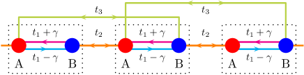
Figure 1: (Color online) The hopping amplitudes of the non-Hermitian SSH model. The dotted boxes indicate the unit cells. For $t_{3}\neq 0$, the eigenvalue equation becomes quartic form, and the generalized Brillouin zone is not necessarily a simple circle in the complex $\beta$ plain (see Fig. 2).

The Bloch Hamiltonian is

$$H(k)=(t_{1}+t_{2}\cos k)\tau_{x}+(t_{2}\sin k+{\rm i}\gamma)\tau_{y},$$ (6)

where $\tau_{\mu}\,(\mu=x,y,z)$ are Pauli matrices. Then the eigenvalue is given by

$$\varepsilon_{\pm}(k) =\pm\sqrt{t_{1}^{2}+t_{2}^{2}-\gamma^{2}+2t_{2}(t_{1}\cos k+{\rm i}\gamma\sin k)}.$$ (7)

The energy gap closes at $t_{1}=\pm(t_{2}\pm\gamma)$. When $\gamma=0$, this model is Hermitian, and phase transitions occur at $t_{1}=\pm t_{2}$. In this case, the orthogonality of eigenstates excludes this non-Hermitian skin effect. However, for $\gamma\neq 0$, the system may show the non-Hermitian skin effect due to the asymmetry of the hopping amplitude and open boundary conditions.

3.2 Polarization for $t_{3}=0$

In order to see the non-Hermitian skin effect, we apply the procedure of the non-Bloch band theory to the Bloch Hamiltonian [13, 15]. By the replacement $\beta={\rm e}^{{\rm i}k}\,(k\in\mathbb{C})$ in Eq. (6), we obtain the non-Bloch Hamiltonian as

$$H(\beta)=\begin{pmatrix}&h_{+}(\beta)\\ h_{-}(\beta)&\end{pmatrix},$$ (8)

where $h_{\pm}(\beta)=t_{1}\pm\gamma+t_{2}\beta^{\mp 1}$. In the non-Bloch band theory, we treat the eigenvalue equation ${\rm det\,}[H(\beta)-E]=0$ as the algebraic equation in terms of $\beta$. Considering the condition $|\beta_{1}|=|\beta_{2}|$, where $\beta_{1,2}$ are solutions of the eigenvalue equation, we get the generalized Brillouin zone $C_{\beta}$:

$$\beta_{1,2}=r{\rm e}^{{\rm i}\tilde{k}},$$ (9)

where $r=\sqrt{|(t_{1}-\gamma)/(t_{1}+\gamma)|}$, and $\tilde{k}\in\mathbb{R}$. For $t_{3}\neq 0$, the eigenvalue equation becomes quartic form, and the generalized Brillouin zone $C_{\beta}$ is not necessarily a simple circle in the complex $\beta$ plain (see Fig. 2).

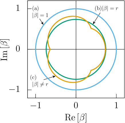
Figure 2: (Color online) (a) The Brillouin zone for $\gamma=0$ and (b,c) the generalized Brillouin zone $C_{\beta}$ plotted in the $\beta$ plain. Parameters are (b) $t_{1}=1.7,t_{2}=1,t_{3}=0,\gamma=0.5$, and (c) $t_{1}=0.3,t_{2}=0.8,t_{3}=0.2,\gamma=0.5$.

The polarization which is given by Eq. (4) is extended to the non-Bloch Hamiltonian using $\tilde{k}$ instead of $k$, which is discretized as $\tilde{k}=(2\pi/N_{\beta})n$ for $n=0,1,\cdots,N_{\beta}-1$:

$$z^{(1)}_{\beta}=(-1)\prod_{n=0}^{N_{\beta}-1}\,\braket{u^{\rm L}_{\tilde{k}_{n+1}-}}{u^{\rm R}_{\tilde{k}_{n}-}},$$ (10)

where we choose $q=1$ because $N=L$ in the present model. Note that $N_{\beta}$ is not the system size $L$ but the number of grid points on $C_{\beta}$. Hereafter, we call $z^{(1)}_{\beta}$ “non-Bloch polarization.” It can be shown that $z^{(1)}_{\beta}$ is real by pseudo Hermiticity of the system.

On the other hand, it is already known that the non-Hermitian skin effect is characterized by the non-Bloch winding number [13]. Since Eq. (8) has chiral symmetry $\tau_{z}H(\beta)\tau_{z}=-H(\beta)$, the non-Bloch winding number is introduced as

$$w=\frac{{\rm i}}{2\pi}\int_{C_{\beta}}{\rm d}s\,s^{-1},$$ (11)

where $s(\beta)=h_{+}(\beta)/\sqrt{h_{+}(\beta)h_{-}(\beta)}$. As discussed in Ref. 7, there is a correspondence between the winding number $w$ and the polarization $z$ in Hermitian systems. Therefore the same relation is expected to be satisfied for the non-Bloch polarization as

$$w=1-\frac{1}{\pi}{\rm Im}\,\ln z^{(1)}_{\beta}$$ (12)

for $N_{\beta}\to\infty$. It is easy to check this correspondence for $t_{3}=0$ where the radius of the generalized Brillouin zone $C_{\beta}$ is a circle with fixed $r$. However, for $t_{3}\neq 0$, this relation is nontrivial.

In Fig. 3, we show the numerical results for $t_{3}=0$. We find that the sign of the polarization $z^{(1)}_{\beta}$ defined on the generalized Brillouin zone changes at transition points $t_{1}=\pm\sqrt{t_{2}^{2}+\gamma^{2}}$, and $z^{(1)}_{\beta}=1$ in the region with the zero modes $|E|=0$ and $w=1$, reflecting the non-Hermitian skin effect [13]. Whereas $w$ is defined except at the transition points, $z^{(1)}_{\beta}$ is a continuous quantity. Therefore, $z^{(1)}_{\beta}$ is more convenient quantity to detect the phase transition points than $w$, especially in numerical analysis.

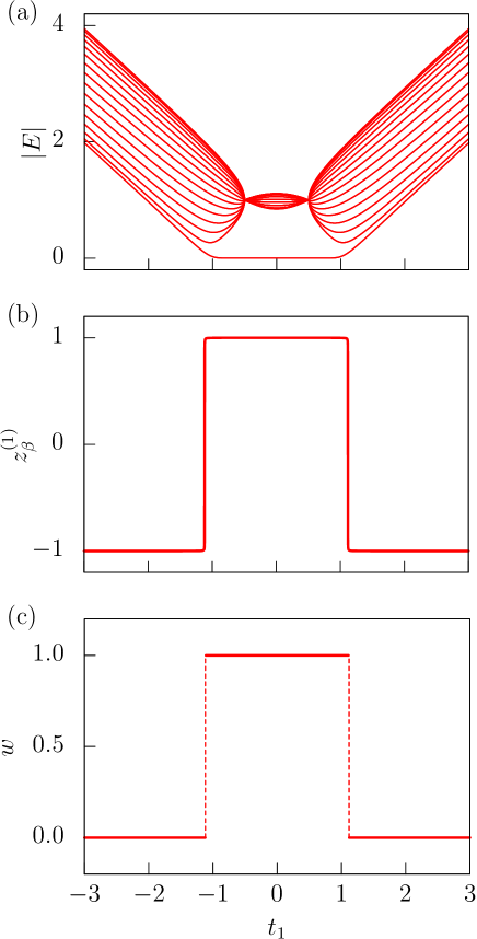
Figure 3: (Color online) (a) The absolute value of eigenvalues, (b) the non-Bloch polarization and (c) the non-Bloch winding number in the non-Hermitian SSH model with $t_{2}=1,\gamma=0.5$ and $t_{3}=0$. The eigenvalues are computed for $L=16$ with open boundary conditions, and the polarization is calculated for $N_{\beta}=8192$. Phase transition points are $|t_{1}|=\sqrt{t_{2}^{2}+\gamma^{2}}\simeq 1.12$. For $|t_{1}|<\sqrt{t_{2}^{2}+\gamma^{2}}$, the zero modes appear in the spectra, and the winding number takes $w=1$ reflecting the non-Hermitian skin effect as discussed in Ref. 13. In addition to these, $z^{(1)}_{\beta}$ changes the sign at the same points.

3.3 Polarization for $t_{3}\neq 0$

For $t_{3}\neq 0$, we can also calculate the polarization $z^{(1)}_{\beta}$ and show that the results coincide with those obtained by the winding number $w$ [13]. We explain how to find the generalized Brillouin zone in this case following Ref. 15. We assume that two solutions, which are $\beta$ and $\beta^{\prime}=\beta{\rm e}^{{\rm i}\theta}$, satisfy the eigenvalue equations:

$$h_{+}(\beta)h_{-}(\beta)=E^{2},\quad h_{+}(\beta{\rm e}^{{\rm i}\theta})h_{-}(\beta{\rm e}^{{\rm i}\theta})=E^{2},$$ (13)

where $\theta$ is an arbitrary constant. Then we obtain

$$h_{+}(\beta)h_{-}(\beta)-h_{+}(\beta{\rm e}^{{\rm i}\theta})h_{-}(\beta{\rm e}^{{\rm i}\theta})=0,$$ (14)

which is independent of $E$. By fixing $\theta$, we solve the above equation and label the four solutions as $|\beta_{1}|\leq|\beta_{2}|\leq|\beta_{3}|\leq|\beta_{4}|$. According to the non-Bloch band theory, the trajectory given by the condition $|\beta_{2}|=|\beta_{3}|$ is the generalized Brillouin zone $C_{\beta}$, which is not a circle in general (see Fig. 2). For $C_{\beta}$ which is a closed loop, we label each $\beta$’s of $N_{\beta}$ grid points as

$$0\leq{\rm arg\,}\beta^{(1)}<{\rm arg\,}\beta^{(2)}<\cdots<{\rm arg\,}\beta^{(N_{\beta})}<2\pi.$$ (15)

Then we introduce the polarization defined on $C_{\beta}$ as follows:

$$z^{(1)}_{\beta}=(-1)\prod_{n=1}^{N_{\beta}}\,\braket{u^{\rm L}_{\beta^{(n+1)}-}}{u^{\rm R}_{\beta^{(n)}-}},$$ (16)

where $\ket{u^{\rm R(L)}_{\beta-}}$ is the right (left) eigenstate of $H(\beta)$, and $\beta^{(N_{\beta}+1)}\equiv\beta^{(1)}$. When $C_{\beta}$ is a circle, Eq. (16) is reduced to Eq. (10).

In Fig. 4, we show the absolute value of eigenvalues $|E|$ and the polarization $z^{(1)}_{\beta}$ for $t_{3}\neq 0$. In this case, the results also show that the correspondence exists between the zero modes in the spectra and $z^{(1)}_{\beta}$. There is also a relation between winding number $w$ and $z^{(1)}_{\beta}$ as Eq. (12).

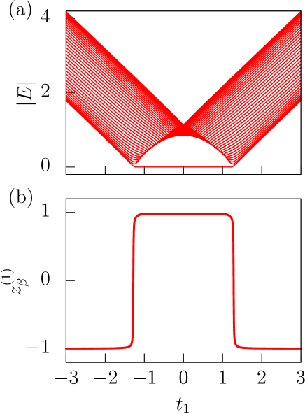
Figure 4: (Color online) (a) The absolute value of the eigenvalues for $L=40$ and (b) the polarization for $N_{\beta}=200$ with $t_{2}=1,t_{3}=0.2,\gamma=0.3$. $z^{(1)}_{\beta}$ changes the sign at the same points where the zero modes appear in the spectra.

4 2D non-Hermitian skin effect

As a model of 2D systems, we consider the WD model [40, 41] including the non-Hermitian term (imaginary Zeeman field) as follows [14]:

$$H(\bm{k})=H_{\rm WD}(\bm{k})+{\rm i}\sum_{\mu=x,y}\gamma_{\mu}\tau_{\mu},$$ (17)

$$H_{\rm WD}(\bm{k})=t\sum_{\mu=x,y}\sin k_{\mu}\tau_{\mu}+d_{z}\tau_{z},$$ (18)

where

$$d_{z}=M-B\sum_{\mu=x,y}\cos k_{\mu}.$$ (19)

Then the eigenvalues are given by

$$\varepsilon_{\pm}(\bm{k})=\pm\sqrt{\sum_{\mu=x,y}(t\sin k_{\mu}+{\rm i}\gamma_{\mu})^{2}+d_{z}^{2}}.$$ (20)

When $\gamma_{\mu}=0$, this system is Hermitian, and phase transitions occur at $B=\pm M/2$, where the energy gap closes.

In order to simplify this model, we need the following three steps. First, we consider the continuum version of Eq. (18) using the Taylor expansion around $k_{\mu}=0$ as,

$$H_{\rm cont.}(\bm{k})= \sum_{\mu=x,y}(tk_{\mu}+{\rm i}\gamma_{\mu})\tau_{\mu}$$

$$+\left[M-2B+\frac{B}{2}(k_{x}^{2}+k_{y}^{2})\right]\tau_{z}.$$ (21)

Next, considering the $\gamma_{\mu}$-term as a perturbation, the relevant eigenstate of $H_{\rm cont.}$ is exponentially localized which corresponds to the non-Hermitian skin effect. By the replacement $k_{\mu}\to\tilde{k}_{\mu}-{\rm i}\gamma_{\mu}/t$, we then obtain the non-Bloch Hamiltonian

$$\tilde{H}_{\rm cont.}(\tilde{\bm{k}})= t\tilde{k}_{x}\tau_{x}+t\tilde{k}_{y}\tau_{y}+\tilde{d}_{z}\tau_{z}$$

$$-\frac{B}{t}\sum_{\mu=x,y}\left(\frac{\gamma_{\mu}^{2}}{2t}+{\rm i}\gamma_{\mu}\tilde{k}_{\mu}\right)\tau_{z},$$ (22)

where

$$\tilde{d}_{z}=M-B\sum_{\mu=x,y}\left(1-\frac{\tilde{k}_{\mu}^{2}}{2}\right).$$ (23)

Finally, we restore the continuum model Eq. (22) to the lattice model as follows:

$$\tilde{H}(\tilde{\bm{k}})=H_{\rm WD}(\tilde{\bm{k}})-\frac{B}{t}\sum_{\mu=x,y}\left(\frac{\gamma_{\mu}^{2}}{2t}+{\rm i}\gamma_{\mu}\sin\tilde{k}_{\mu}\right)\tau_{z},$$ (24)

where $H_{\rm WD}$ is defined by Eq. (18), and we set $\gamma_{x}=\gamma_{y}=\gamma$. The energy gap closes at $B=M/(2+\gamma^{2}/t^{2})$. Hereafter, we analyze the model (24) instead of Eq. (17).

The phases appearing in the 2D WD model $H_{\rm WD}(\bm{k})$ are topologically distinguished by the Chern number which is defined on the conventional Brillouin zone. Instead of this, the phases of $\tilde{H}(\tilde{\bm{k}})$ are characterized by the non-Bloch Chern number [14]

$$\nu=\frac{2\pi}{L_{x}L_{y}}\sum_{\tilde{\bm{k}}}\left(\frac{\partial A_{y}(\tilde{\bm{k}})}{\partial\tilde{k}_{x}}-\frac{\partial A_{x}(\tilde{\bm{k}})}{\partial\tilde{k}_{y}}\right),$$ (25)

where $\tilde{k}_{\mu}=(2\pi/L_{\mu})n_{\mu}$ for $(n_{\mu}=0,1,\cdots,L_{\mu}-1)$, and $A_{\mu}(\tilde{\bm{k}})=-{\rm i}\braket{u^{\rm L}_{\tilde{\bm{k}}-}}{\partial_{\tilde{k}_{\mu}}u^{\rm R}_{\tilde{\bm{k}}-}}$.

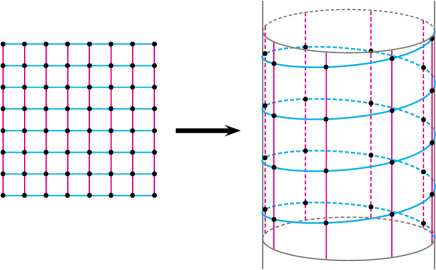
Figure 5: (Color online) SBCs for a 2D square lattice where the system is represented as a projected 1D chain (blue lines). The parameter $\Lambda$ is the hopping range $c_{i+\Lambda,\alpha}^{{\dagger}}c_{i,\alpha}^{\mathstrut}+\mbox{H.c.}$ of the 1D chain originating from the hopping along the $y$ direction (magenta lines). This is also related to the circumference of the torus.

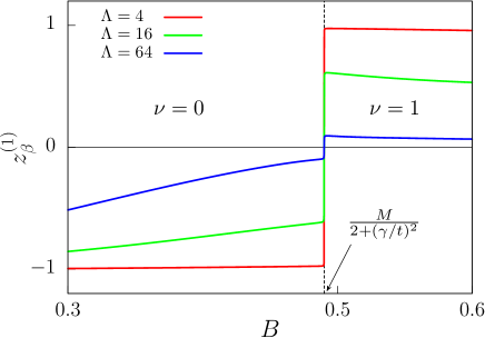
Figure 6: (Color online) The non-Bloch polarization (10) of the effective lattice model of the non-Hermitian WD model given by Eq. (24). The parameters are $t=M=1$, $\gamma_{x}=\gamma_{y}=\gamma=0.2$, $N_{\beta}=2^{20}$, and $\Lambda=4,16,64$. The transition point is $B=M/(2+\gamma^{2}/t^{2})\simeq 0.490$. The non-Bloch Chern number $\nu$ is defined by Eq. (25).

In addition to this, we also introduce the non-Bloch polarization for 2D systems. For this purpose, we use SBCs that sweep all lattices in 1D orders as illustrated in Fig. 5 [42, 38]. When we apply SBCs to 2D lattice models, the 2D wave numbers $(k_{x},k_{y})$ are replaced by $(k,\Lambda k)$, where $k$ is the wave number of the projected 1D chain, and the parameter $\Lambda$ is the range of the hopping $c_{i+\Lambda,\alpha}^{{\dagger}}c_{i,\alpha}^{\mathstrut}+\mbox{H.c.}$ related with a hopping to $y$-direction in the original 2D lattice [38]. It has been shown that the 2D polarization defined in this way becomes $z^{(1)}=0$ at the topological transition points [38] that are also ensured by the LSM theorem extended to higher dimensions [43, 44, 42]. Then we can introduce the 2D non-Bloch polarization $z^{(1)}_{\beta}$ as in the same procedure as in 1D cases using Eq. (10).

In Fig. 6, we show the numerical result of the non-Bloch polarization $z^{(1)}_{\beta}$ of the effective lattice model of the non-Hermitian WD model given by Eq. (24). Here, for the $\tilde{\bm{k}}$ space, we have imposed SBCs for the 2D system and PBCs for the projected 1D chain to use Eq. (10). For large and fixed number of the grid points $N_{\beta}$, the point where $z^{(1)}_{\beta}=0$ has very small $\Lambda$ dependence, and $|z^{(1)}_{\beta}|$ tends to converge to 1 for small $\Lambda$. In the present case, $\Lambda$ is nothing but the circumference of the torus. Therefore it is convenient to calculate $z^{(1)}_{\beta}$ near the thin-torus region, to detect the transition point. The non-Bloch Chern number $\nu$ defined by Eq. (25) takes different values on each sides of the transition point $B=M/(2+\gamma^{2}/t^{2})$, where the sign of $z^{(1)}_{\beta}$ changes. Thus we can detect the non-Hermitian skin effect in 2D by the non-Bloch polarization $z^{(1)}_{\beta}$, similarly to the non-Bloch Chern number $\nu$.

5 Summary and discussion

In summary, we have extended Resta’s electronic polarization to characterize insulating states to the non-Hermitian skin effect in 1D and 2D systems. The extension has been done by rewriting the polarization in the Bloch state and applying the non-Bloch band theory which extends the wave numbers to the complex plain. This enables Resta’s formalism for the electronic polarization in periodic systems to detect non-Hermitian skin effect in open boundary systems. Furthermore, for 2D systems, we have introduced SBCs which sweep all lattice sites in 1D order. Then the non-Bloch electronic polarization defined in 1D lattice systems has been extended to 2D systems, and it also detects the transition point for the non-Hermitian skin effect.

We have demonstrated these arguments in the 1D non-Hermitian SSH model and the 2D non-Hermitian WD model, and found that the regions of the skin effect identified by the non-Bloch electronic polarization are consistent with those obtained by the non-Bloch winding number and the Chern number, respectively. We also show the consistency of the results in more general cases of the non-Hermitian SSH model where the generalized Brillouin zone $C_{\beta}$ is not necessarily a simple circle.

There are some works that claim the polarization defined in periodic systems may detect the phase transition relating the non-Hermitian skin effect [25, 45, 46]. In these works, the numerical results of $\tfrac{1}{\pi}{\rm Im}\,\ln z^{(1)}$ of the non-Hermitian SSH model with PBCs seem to behave similarly to our result of Fig. 3(c). However, this coincidence is accidental one due to the finite-size effect: As shown in our previous work [39], $z^{(1)}$ of the non-Hermitian SSH with PBCs in the thermodynamic limit takes three values. This means that a finite region with $z^{(1)}=0$ exists between two gapped phases with $z^{(1)}=\pm 1$. In the region with $z^{(1)}=0$, Resta’s polarization $\tfrac{1}{\pi}{\rm Im}\,\ln z^{(1)}$ does not have physical meaning as in gapless cases. On the other hand, if one extracts the sign of $z^{(1)}$ in finite-size systems by abusing the relation $\tfrac{1}{\pi}{\rm Im}\,\ln z_{L}^{(1)}$, then it takes only two values 0 or 1 because $z_{L}^{(1)}$ is real and finite. Thus the phase with $z^{(1)}=0$ is overlooked in the periodic cases. In the end, we need the present extension of the electronic polarization by the non-Bloch band theory to deal with the non-Hermitian skin effect.

There is another topological index “biorthogonal polarization” proposed in Refs. 23, 24. This quantity characterizes the number of zero modes [24], and relationship to the non-Bloch winding numbers and the non-Bloch polarization is not fully understood. Since this quantity is defined in the real space with open boundary conditions, our non-Bloch polarization is considered to have an advantage for calculation in larger size systems.

There is another topological index “biorthogonal polarization” proposed in Refs. 23, 24. This quantity characterizes the number of zero modes, [24], and relationship to the non-Bloch winding numbers and the non-Bloch polarization is not fully understood. Since this quantity is defined in the real space with open boundary conditions, our non-Bloch polarization is considered to have an advantage for calculation in larger size systems and for the comprehension of the bulk-boundary correspondence.

6 Acknowledgment

The authors thank N. Hatano, K. Imura, and M. Oshikawa for discussions. M. N. acknowledges the Visiting Researcher’s Program of the Institute for Solid State Physics, the University of Tokyo, and the research fellow position of the Institute of Industrial Science, the University of Tokyo. M. N. is supported partly by JSPS KAKENHI Grant Number 20K03769.

References

- [1] F. D. M. Haldane, Phys. Rev. Lett. 61, 2015 (1988).
- [2] C. L. Kane and E. J. Mele, Phys. Rev. Lett. 95, 146802 (2005).
- [3] Liang Fu, C. L. Kane, and E. J. Mele Phys. Rev. Lett. 98, 106803 (2007).
- [4] B. A. Bernevig and S. C. Zhang, Phys. Rev. Lett. 96, 106802 (2006).
- [5] B. A. Bernevig, T. L. Hughes, and S. C. Zhang, Science 314, 1757 (2006).
- [6] A. P. Schnyder, S. Ryu, A. Furusaki, and A. W. W. Ludwig Phys. Rev. B 78, 195125 (2008).
- [7] S. Ryu, A. P. Schnyder, A. Furusaki, and A.W. Ludwig, New J. Phys. 12, 065010 (2010).
- [8] M. König, S. Wiedmann, C. Brüne, A. Roth, H. Buhmann, L. W. Molenkamp, X.-L. Qi, and S.-C. Zhang, Science, 318, 766 (2007).
- [9] M. König, H. Buhmann, L. W. Molenkamp, T. Hughes, C.-X. Liu, X.-L. Qi, and S.-C. Zhang, J. Phys. Soc. Jpn. 77, 031007 (2008).
- [10] K. Esaki, M. Sato, K. Hasebe, and M. Kohmoto, Phys. Rev. B 84, 205128 (2011).
- [11] T. E. Lee, Phys. Rev. Lett. 116, 133903 (2016).
- [12] H. Shen, B. Zhen, and L. Fu, Phys. Rev. Lett. 120, 146402 (2018).
- [13] S. Yao and Z. Wang, Phys. Rev. Lett. 121, 086803 (2018).
- [14] S. Yao, F. Song, and Z. Wang, Phys. Rev. Lett. 121, 136802 (2018).
- [15] K. Yokomizo and S. Murakami, Phys. Rev. Lett. 123, 066404 (2019).
- [16] K. Kawabata, N. Okuma, M. Sato, symplectic class, Phys. Rev. B 101, 195147 (2020).
- [17] Z. Gong, Y. Ashida, K. Kawabata, K. Takasan, S. Higashikawa, and M. Ueda, Phys. Rev. X 8, 031079 (2018).
- [18] K. Kawabata, K. Shiozaki, M. Ueda, and M. Sato, Phys. Rev. X 9, 041015 (2019).
- [19] N. Okuma, K. Kawabata, K. Shiozaki, and M. Sato, Phys. Rev. Lett. 124, 086801 (2020).
- [20] D. S. Borgnia, A. J. Kruchkov, and R.-J. Slager Phys. Rev. Lett. 124, 056802 (2020).
- [21] P. M. Vecsei, M. M. Denner, T. Neupert, and F. Schindler, Phys. Rev. B 103, L201114, (2021).
- [22] L. Li, S. Mu, C. H. Lee, and J. Gong, Nat. Commun. 12, 5294 (2021).
- [23] F. K. Kunst, E. Edvardsson, J. C. Budich, and E. J. Bergholtz, Phys. Rev. Lett. 121, 026808 (2018).
- [24] E. Edvardsson, F. K. Kunst, T. Yoshida, and E. J. Bergholtz, Phys. Rev. Research 2, 043046 (2020).
- [25] E. Lee, H. Lee, and B.-J. Yang, Phys. Rev. B 101, 121109 (2020).
- [26] R. Resta, Rev. Mod. Phys. 66, 899 (1994).
- [27] R. Resta, Phys. Rev. Lett. 80, 1800 (1998).
- [28] R. Resta and S. Sorella, Phys. Rev. Lett. 82, 370 (1999).
- [29] R. Resta, J. Phys. Condens. Matter 12, R107 (2000).
- [30] E. Lieb, T. Schultz, and D. Mattis, Ann. Phys. (NY) 16, 407 (1961).
- [31] I. Affleck and E. H. Lieb, Lett. Math. Phys. 12, 57 (1986).
- [32] I. Affleck, Phys. Rev. B 37, 5186 (1988).
- [33] M. Oshikawa, M. Yamanaka, and I. Affleck, Phys. Rev. Lett. 78, 1984 (1997).
- [34] M. Yamanaka, M. Oshikawa, and I. Affleck, Phys. Rev. Lett. 79, 1110 (1997).
- [35] A. A. Aligia and G. Ortiz, Phys. Rev. Lett. 82, 2560 (1999).
- [36] M. Nakamura and J. Voit, Phys. Rev. B 65, 153110 (2002).
- [37] M. Nakamura and S. Todo, Phys. Rev. Lett. 89, 077204 (2002).
- [38] M. Nakamura, S. Masuda, and S. Nishimoto, Phys. Rev. B 104, L121114 (2021).
- [39] S. Masuda and M. Nakamura, J. Phys. Soc. Jpn. 91, 043701 (2022).
- [40] K. G. Wilson, Phys. Rev. D 10, 2445 (1974).
- [41] X. L. Qi, Y. S. Wu, and S. C. Zhang, Phys. Rev. B 74, 085308 (2006).
- [42] Y. Yao and M. Oshikawa, Phys. Rev. X 10, 031008 (2020).
- [43] M. Oshikawa, Phys. Rev. Lett. 84, 1535 (2000).
- [44] M. B. Hastings, Europhys. Lett. 70, 824 (2005).
- [45] C. Ortega-Taberner, L. Rodland, and M. Hermanns, Phys. Rev. B 105, 075103 (2022).
- [46] J. Hu, C. A. Perroni, G. De Filippis, S. Zhuang, L. Marrucci, and F. Cardano arXiv:2203.11902.