Tuple Packing:
Efficient Batching of Small Graphs in Graph Neural Networks
Abstract
When processing a batch of graphs in machine learning models such as Graph Neural Networks (GNN), it is common to combine several small graphs into one overall graph to accelerate processing and remove or reduce the overhead of padding. This is for example supported in the PyG library. However, the sizes of small graphs can vary substantially with respect to the number of nodes and edges, and hence the size of the combined graph can still vary considerably, especially for small batch sizes. Therefore, the costs of excessive padding and wasted compute are still incurred when working with static shapes, which are preferred for maximum acceleration. This paper proposes a new hardware agnostic approach —tuple packing— for generating batches that cause minimal overhead. The algorithm extends recently introduced sequence packing approaches to work on the 2D tuples of . A monotone heuristic is applied to the 2D histogram of tuple values to define a priority for packing histogram bins together with the objective to reach a limit on the number of nodes as well as the number of edges. Experiments verify the effectiveness of the algorithm on multiple datasets.
1 Introduction
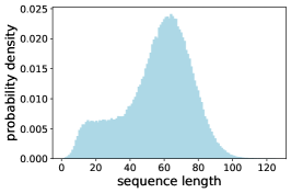
Small graphs can be obtained from a variety of data sources
(for example text, audio, and molecules).
As shown in Figure 1, the resulting length of data (number of nodes) can vary substantially.
The resulting padding can have a significant impact on transformer models like BERT [4]
and can largely benefit from combining/packing data together [5].
The main advantage of the data packing technique is that it is hardware agnostic
and results in speedup on Intelligence Processing Units (IPUs) by Graphcore [5],
GPUs by NVIDIA 111BERT sequence packing section at:
https://developer.nvidia.com/blog/boosting-mlperf-training-performance-with-full-stack-optimization/,
and Gaudi by Intel/Habana 222https://developer.habana.ai/tutorials/tensorflow/data-packing-process-for-mlperf-bert/.
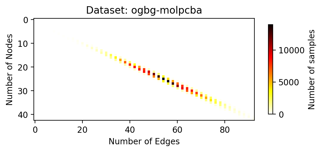
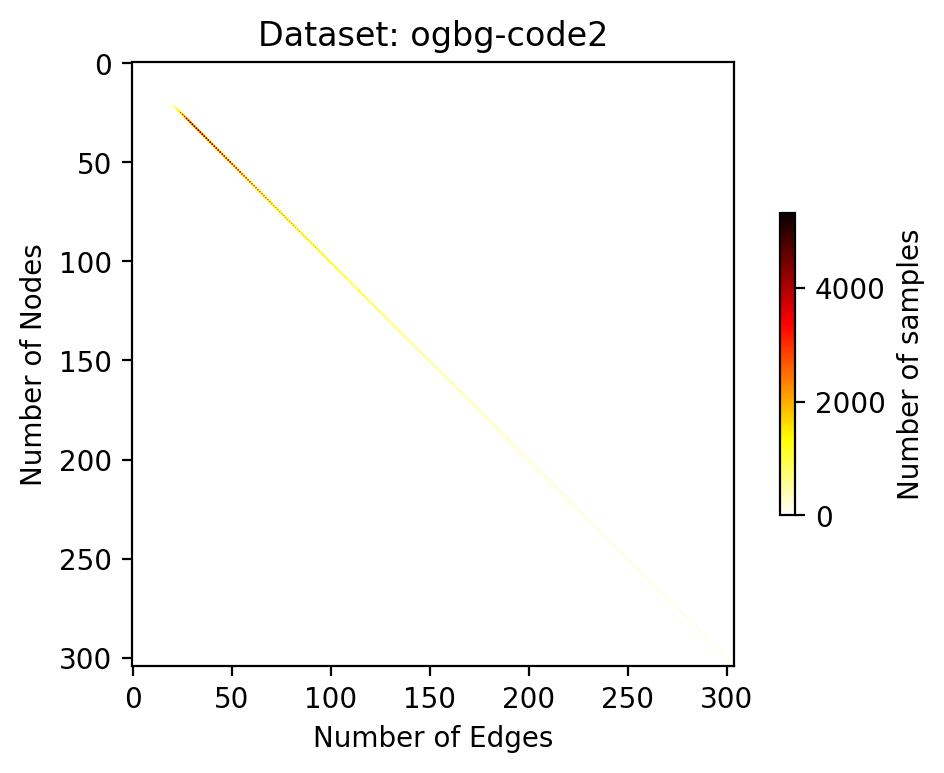
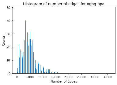
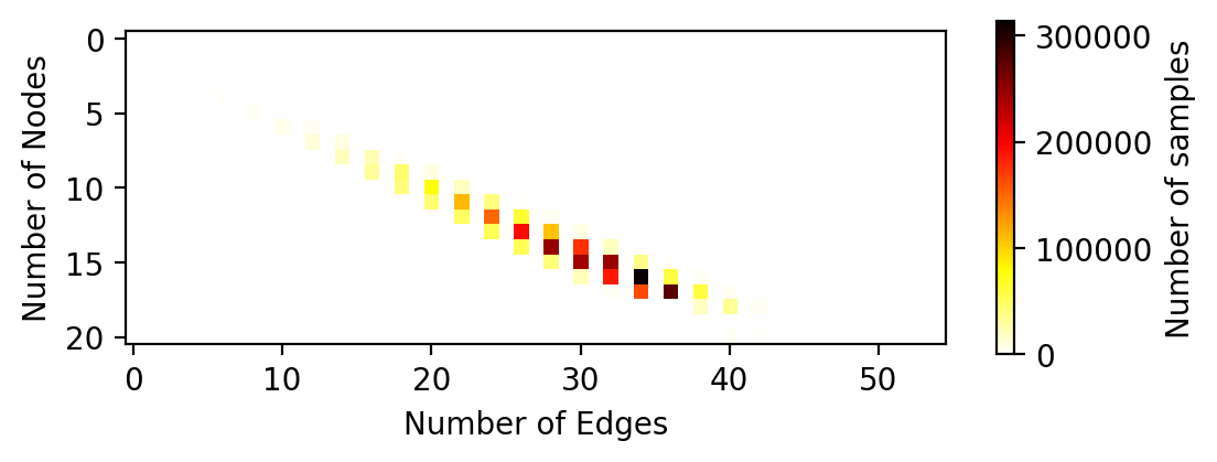
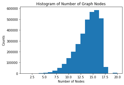
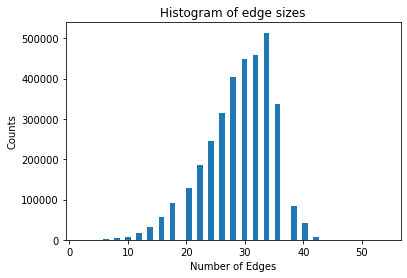
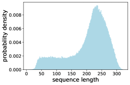
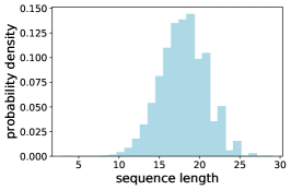
In this paper, we focus our application on Open Graph Benchmark (OGB) datasets for graph property prediction [6] 333https://ogb.stanford.edu/docs/graphprop/ as well as the PCQM4Mv2 dataset [7] that is part of the OGB large scale competition [8] 444https://ogb.stanford.edu/docs/lsc/pcqm4mv2/. The histograms are provided in Figure 2 and Figure 3 respectively. In some cases, the long tails of the distributions were cut off for better visualization. Statistics are provided in Table 1. The node-edge length count describes how many different combinations of the number of edges and nodes exist in the dataset. Further datasets and statistics are described on the PyG webpage 555https://pytorch-geometric.readthedocs.io/en/latest/notes/data_cheatsheet.html. We used PyG to obtain the data distributions for the experiments in this paper.
| ogbg-datasets | |||||
| Metric | molhiv | molpcba | code2 | pcqm4mv2 | ppa |
| Number of (training) graphs | 32901 | 350343 | 407976 | 3378606 | 78200 |
| Max number of nodes | 222 | 313 | 36123 | 20 | 300 |
| Max number of edges | 502 | 636 | 36122 | 54 | 36138 |
| Node-edge length count | 795 | 576 | 2099 | 152 | 35981 |
| Node efficiency (%) | 11.4 | 8.21 | 0.35 | 27.7 | 81.1 |
| Edge efficiency (%) | 10.8 | 8.71 | 0.34 | 24.7 | 12.6 |
| Potential speedup for nodes | 8.8 | 12.2 | 288.8 | 3.6 | 1.23 |
| Potential speedup for edges | 9.3 | 11.5 | 291.2 | 4.1 | 7.95 |
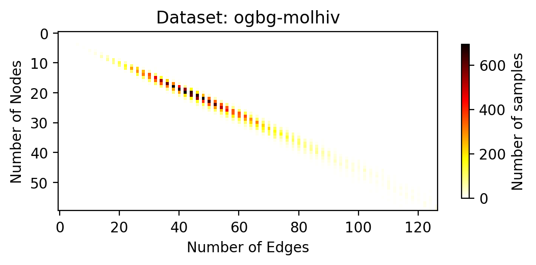
In all cases, a substantial amount of padding for the nodes and edges is required in order to obtain equally sized batches. Apart from the PPA dataset, we can observe an almost linear relationship between the number of edges and the number of nodes. Hence, two questions arise: firstly, can we generalise the packing concept introduced for BERT [5] to tuples? This question is addressed in Section 2. Secondly, how much benefit would a tuple packing approach provide compared to solely focusing the packing on edges or nodes and applying classical packing? This is addressed in Section 3. We summarize and provide an outlook in Section 4.
2 Methods
2.1 Single Sequence Packing
“The bin packing problem deals with the assignment of items into bins of a fixed capacity such that the number of utilized bins is minimized. In the canonical formulation of the packing problem a vector of length is used to represent the items being packed, where denotes the length of the i-th sequence/item. The allocation of items into bins is tracked through the assignment matrix , where states whether the i-th sequence should be placed into the j-th bin. In the worst case scenario, every item is assigned to its own bin, thus . Notably, grows linearly in the number of sequences/items being packed and grows with the square. To mask out unused bins , denotes whether the j-th bin is being used. The optimization objective is to minimize the sum of while making sure to assign each to exactly one bin and not exceeding the maximum bin capacity [constant] for each bin. [The index m stands for .] This problem formulation is well known as bin packing [9].”[5]
| Minimize the number of bins. | (1) | ||||
| s.t. | Assign each length/sequence to only one bin. | ||||
| Cumulative length cannot exceed capacity. |
As discussed by Kosec et al. [5], this problem can be simplified by working on histograms instead. It can be solved either by casting it to a non-negative least squares problem, or by using simple heuristics to directly derive a solution (for example by applying first-fit decreasing or best-fit on the histograms). Note that there are two heuristics present. The first, more trivial one, decides how we sort the incoming sequences, which is most efficient when going from longest to shortest. The second heuristic decides how we measure the remaining space and how to sort bins that are not yet full. Again, we can only use the sequence length of the remaining space in the bin. However, first-fit sorts the remainder from longest to smallest and best-fit uses the reverse order. For tuples of sequences, this becomes more challenging. More sophisticated heuristics are required to reduce the tuple of sequence lengths to a single number which is used to decide the packing priority.
2.2 Tuple Packing
Tuple packing means that instead of items with length (size) , we have a tuple of lengths
for a l-tuple of items that need to be packed up to a maximum capacity per component of the tuple:
| Minimize the number of bins. | (2) | ||||
| s.t. | Assign each length/sequence to only one bin. | ||||
| Cumulative length cannot exceed capacity. |
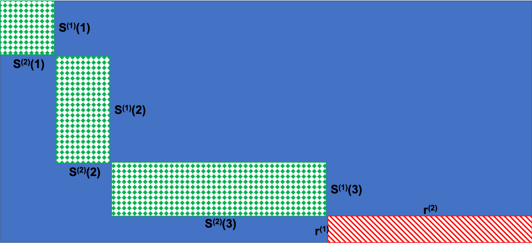
Note that the number of parameters does not change but the number of constraints does. Thus the higher the , the more challenging it is to find a good solution. Also note that when considering a vector/matrix notation for the inequality in Equations 2, it is equivalent to Equation 1 Tuple packing is simpler than k-dimensional packing as shown in Figure 4 where . Instead of filling a full rectangle, we are only packing along the “diagonal” and the remaining lower rectangle has to be minimized.
In practice, we are less interested in minimizing the number of bins but we want the sum of
to be as small as possible for each . In other words, we want to have as little padding as possible in order to reach the maximum capacity in each tuple component. Note, however, that solving the optimization problem will provide the same result for both objectives because the fewer bins we have, the less padding we encounter.
2.3 Heuristics
For single sequence packing, the objective is clearly to minimize the single padding value, however the existence of a packing tuple for each bin requires some compromises. Our proposal is to use a monotonically increasing heuristic that is zero when there is no remainder. Examples are and their weighted counterparts. For pair packing, monotonically increasing means that if and it holds . Strictly monotone means that if and (or and ) it holds . The functions and do not fulfill the strict condition but are monotone. The product is strictly monotone as long as no factor is zero. The sum is strictly monotone. Also the projection onto one component is monotone and would reduce the problem to the well known bin-packing if no limit for the other components is set.
2.4 Tuple longest-pack-first histogram-packing
Together with the heuristic, we propose a new variant of Best-Fit Bin Packing [10, 11] applied to a histogram in descending order (also known as longest-pack-first histogram-packing).
When packing simple sequences, we can sort by the sequence length, however in this example, we need the heuristics. Hence, we sort the incoming bins of node-edge pairs and respective counts based on heuristics. This means that multiple tuples can obtain the same heuristic and sorting might be not deterministic. For example, for the heuristic (as well as the unweighted heuristics ), the pairs and get the same heuristic value of . Originally, for Best-Fit, we chose the fullest existing pack that could still fit the incoming bin. The term “pack” is used here to refer to a set of length tuples that were combined and their respective count of occurrence. This time, each existing pack comes with a remainder in each component, that can still be filled (the tuple of described above). We apply the same heuristic to each remainder of existing packs. Next, we iterate from the bins starting with the value of the heuristic of the incoming bin up to the maximum value of the heuristic applied to the length limits . For each value, we iterate over all respective existing packs and check separate if the bin fits in. For the single sequence algorithms, this check was always true and thus not required. If the bin fits, it gets added to the pack and its respective count gets split and reduced. If the count is not zero, the search starts anew from the beginning, since the modification of the pack might have created a new pack that can fit the incoming bin multiple times. If the bin cannot fit in any pack, a new pack is created that includes only the bin.
It is also possible to implement a First-Fit variant (also called tuple shortest-pack-first histogram-packing). The algorithm is exactly the same but starts with the packs with the largest value of the heuristic down to the smallest, because the “shortest” pack will have the largest remainder.
Since the algorithms iterate on histograms instead of each item, they can return a packing proposal within milliseconds if the number of bins is small. This is crucial to iterate over different limits for . Compared to the sequence packing of the original algorithm [5], the complexity of tuple packing is at least as high (the number of sequences squared) with the maximum sequence length now replaced by the number of possible combinations of edges and nodes. The number of possible combinations can be considerably higher compared to sequence packing in BERT. A more detailed complexity analysis is planned to investigate this.
2.5 Choice of length limits
For Natural Language Processing algorithms like BERT, the maximum sequence length is fixed and cannot be adjusted for packing because it would increase computing and memory requirements quadratically and thus suppress any speedup from packing. For GNNs, the cost is usually linear, and thus, the pack limits for tuples, , can be adjusted to requirements of the hardware as well as the packing efficiency. So for example, instead of choosing as the maximum number of nodes of any graph in the dataset and as the maximum number of edges, larger numbers are possible where the limit is usually given either by the hardware or by the processed batch becoming too large and updates happening too frequently.
Given that the packing algorithms provide a solution very quickly, we propose to iterate over all potential combinations of relevant limits from smallest to longest and choose the best trade-off by hand. This could be, for example, the smallest combination (calculated by the heuristic) that achieves a certain packing efficiency (say ) either on average or for each component. Note that starting with the maximums in the dataset and increasing each of them step-wise by one is not recommended because it will favor one component and suppress efficiency in the other components.
If the search space is too big, the limits can be linearly scaled until one components reaches high efficiency and then the other components can be optimized. It is also possible, to set no limit for all but one components to get a good start and iterate from a solution that is optimal for one component.
It is future work to determine more automatic search algorithms. Note that any derivative free parameter optimization algorithm can be applied, for example direction search, because a single evaluation can be calculated fast.
2.6 Implementation
Whilst transformers still require extra effort to be made to process packed samples, it is becoming standard for Graph Neural Networks libraries to include the processing of packed samples. For example in PyTorch Geometric (PyG), all the data that needs to be combined is provided as a batch which gets automatically combined and processed as a large graph 666https://pytorch-geometric.readthedocs.io/en/latest/notes/batching.html. The PyG documentation states: “This procedure has some crucial advantages over other batching procedures:
-
1.
GNN operators that rely on a message passing scheme do not need to be modified since messages still cannot be exchanged between two nodes that belong to different graphs.
-
2.
There is no computational or memory overhead. For example, this batching procedure works completely without any padding of node or edge features. Note that there is no additional memory overhead for adjacency matrices since they are saved in a sparse fashion holding only non-zero entries, i.e., the edges.
PyG automatically takes care of batching multiple graphs into a single giant graph with the help of the torch_geometric.loader.DataLoader class.” Note that for obtaining static data shapes, some padding is still required. However, this can be kept to a minimum with a good packing strategy.
A similar approach exists in the JAX JGraph library777https://jraph.readthedocs.io/en/latest/api.html#batching-padding-utilities and the TensorFlow DGL library [12]888https://docs.dgl.ai/en/0.8.x/_modules/dgl/batch.html. In all three libraries, there is a reverse operation to separate the graphs again. The two operations are sometimes called batching and unbatching. Unbatching is for example useful to add a transformer head[13] or to calculate a graph-wise loss. Note that the packing techniques can still be applied with a modified unbatching.
Note that packing can limit the variation in the dataset - the packs get shuffled but the graphs that are combined in a pack might stay fixed. However, there will be still a large amount of variation in the bact. It is also possible to only fix the sizes of graphs that get combined but sample the graphs randomly. The benefit of this techniques largely depends on the dataset. In an informal analysis, we did not observe any negative impact on performance when using packing and there was no noticeable effect from randomizing the content of packs further. This is aligned with the observations in BERT [5]. Further analysis however is required for a more complex study of this technique.
3 Experiments
This section evaluates different aspects of tuple packing such as the choice of heuristic and of length. To evaluate the algorithm, the node and edge efficiencies have to either be provided separately or aggregated in a joint metric.
3.1 Heuristic comparison
In the first set of experiments, we used the maximum number of edges and nodes in the dataset as a limit for the packing and compared different heuristics against baselines. In the first four heuristics, the number of remaining edges and nodes get combined. For the other two heuristics, we projected and only looked at the remaining spots for nodes or edges. Note, that the limits for the nodes and edges are still applied. For the baselines, we considered no packing (None) or applying packing only on one component while totally ignoring the second component (Node base and Edge base). Thus, the maximum number of edges or nodes can be exceeded for the component that is not considered. The results are displayed in Table 2.
| ogbg-datasets | |||||
| Heuristics | molhiv | molpcba | code2 | pcqm4mv2 | ppa |
| Product | (95.6, 90.5) | (89.6, 95.1) | (46.0, 45.6) | (76.1, 58.0) | - |
| Sum | (97.5, 92.4) | (85.4, 90.6) | (46.0, 45.6) | (76.1, 58.0) | - |
| Maximum | (98.5, 93.3) | (92.6, 98.3) | (46.0, 45.6) | (76.1, 58.0) | - |
| Minimum | (98.5, 93.3) | (92.6, 98.3) | (46.0, 45.6) | (76.1, 58.0) | - |
| Node | (98.8, 93.6) | (91.5, 97.1) | (26.0, 25.8) | (75.1, 57.2) | (99.3, 15.4) |
| Edge | (98.5, 93.3) | (90.6, 96.2) | (46.0, 45.6) | (76.1, 58.0) | - |
| Baseline | |||||
| None | (11.4, 10.8) | (8.21, 8.71) | (0.35, 0.34) | (27.7, 24.7) | (81.1, 12.6) |
| Node base | (98.7, 85.9) | (88.3, 84.5) | (26.0, 25.8) | (75.1, 48.3) | (99.3, 15.4) |
| Edge base | (85.8, 93.3) | (81.0, 88.1) | (40.1, 40.1) | (62.7, 76.4) | (32.7, 99.9) |
We did not measure times. However, all the results for molhiv, molpcba, and pcqm4mv2 were obtained in milliseconds. For code2, it took several seconds but less than ten minutes. For ppa, multiple results could not be obtained within this time limit. This is reasonable due to the complexity of the search space: code2 has original bins and up to size combinations, whereas ppa has original bins and potential combinations.
There is no clear favorite heuristic that works for all cases. Tuple packing with the individually best heuristic always improves performance significantly compared to the baselines. However, the original packing algorithms are already effective and the anticipated additional speedup gains from also using tuple packing are mostly around 1.15x.
For pcqm4mv2, results are rather low because of the distribution of the data where the limits on the nodes and edges do not really allow for perfect patting since the majority of graphs is around 15 edges and 30 nodes, whereas our maximum was 20 nodes and 54 edges. Thus setting different limits is of interest. Further investigation with the code2 dataset is required to get a faster packing algorithm that can handle combining more graphs with better efficiency. Note that most graphs in code2 have around nodes and edges whereas the maximum is around nodes and edges. This is a very imbalanced packing scenario where a lot of graphs need to be combined to avoid padding, which explains the comparably low efficiency values.
3.2 Size limit variation
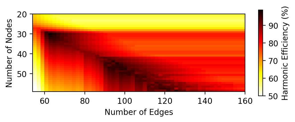
For the PCQM4Mv2 dataset, we observed low efficiency of tuple packing on the edge component (). In this Section, we evaluate the method from Section 2.5 and compare different limits for the number of nodes and edges in a pack. We use the product heuristic on the PCQM4Mv2 dataset with at least nodes and edges. The results are visualized in Figure 5 with the baseline in the upper left corner. Obtaining these results only takes a short amount of time because of the fast packing algorithm. It can be seen that the efficiency can be significantly improved. For visualization purposes we have used the harmonic mean because it is sensitive to the balance of the two constituent efficiencies. The best result was obtained for nodes and edges () with harmonic mean. This is a improvement compared to the previous best result of as the harmonic mean of .
4 Conclusion
In this paper we discuss how a large potion of padding potentially may be required for processing graphs by visualizing multiple datasets. To address this, we introduce a new tuple packing problem and solution. We show that while normal packing (that addresses only one component of the input data) can reduce padding, our tuple packing approach can further improve performance by . Furthermore, by adjusting the limits for edges and nodes, a further improvement has been shown to be possible on the PCQM4Mv2 molecule graph dataset. These improvements in reduced padding can benefit any hardware accelerator, especially when working with static shapes and ahead of time compilation strategies.
For datasets with a large variety of potential node-edge combinations, the complexity of our packing algorithm increases significantly. Future work is planned to speedup the tuple packing algorithm for these kinds of datasets and evaluate the packing approach on Graph Neural Networks to determine, how much speedup can be achieved by reducing the padding.
References
- [1] Vassil Panayotov, Guoguo Chen, Daniel Povey, and Sanjeev Khudanpur. Librispeech: an asr corpus based on public domain audio books. In Acoustics, Speech and Signal Processing (ICASSP), 2015 IEEE International Conference on, pages 5206–5210. IEEE, 2015.
- [2] Lars Ruddigkeit, Ruud van Deursen, Lorenz C. Blum, and Jean-Louis Reymond. Enumeration of 166 billion organic small molecules in the chemical universe database gdb-17. Journal of Chemical Information and Modeling, 52(11):2864–2875, 2012. PMID: 23088335.
- [3] Raghunathan Ramakrishnan, Pavlo O Dral, Matthias Rupp, and O Anatole von Lilienfeld. Quantum chemistry structures and properties of 134 kilo molecules. Scientific Data, 1, 2014.
- [4] Jacob Devlin, Ming Wei Chang, Kenton Lee, and Kristina Toutanova. BERT: Pre-training of deep bidirectional transformers for language understanding. NAACL HLT 2019 - 2019 Conference of the North American Chapter of the Association for Computational Linguistics: Human Language Technologies - Proceedings of the Conference, 1:4171–4186, oct 2019.
- [5] Matej Kosec, Sheng Fu, and Mario Michael Krell. Packing: Towards 2x NLP BERT Acceleration. arXiv, jun 2021.
- [6] Weihua Hu, Matthias Fey, Marinka Zitnik, Yuxiao Dong, Hongyu Ren, Bowen Liu, Michele Catasta, and Jure Leskovec. Open graph benchmark: Datasets for machine learning on graphs. arXiv preprint arXiv:2005.00687, 2020.
- [7] Maho Nakata and Tomomi Shimazaki. Pubchemqc project: A large-scale first-principles electronic structure database for data-driven chemistry. Journal of Chemical Information and Modeling, 57(6):1300–1308, 2017. PMID: 28481528.
- [8] Weihua Hu, Matthias Fey, Hongyu Ren, Maho Nakata, Yuxiao Dong, and Jure Leskovec. Ogb-lsc: A large-scale challenge for machine learning on graphs. arXiv preprint arXiv:2103.09430, 2021.
- [9] Bernhard Korte and Jens Vygen. Combinatorial Optimization, volume 21 of Algorithms and Combinatorics. Springer Berlin Heidelberg, Berlin, Heidelberg, 2012.
- [10] David S Johnson. Near-optimal bin packing algorithms. PhD thesis, Massachusetts Institute of Technology, 1973.
- [11] György Dósa and Jiří Sgall. Optimal analysis of best fit bin packing. In Lecture Notes in Computer Science (including subseries Lecture Notes in Artificial Intelligence and Lecture Notes in Bioinformatics), volume 8572 LNCS PART 1, pages 429–441. Springer Verlag, 2014.
- [12] Minjie Wang, Da Zheng, Zihao Ye, Quan Gan, Mufei Li, Xiang Song, Jinjing Zhou, Chao Ma, Lingfan Yu, Yu Gai, Tianjun Xiao, Tong He, George Karypis, Jinyang Li, and Zheng Zhang. Deep graph library: A graph-centric, highly-performant package for graph neural networks. arXiv preprint arXiv:1909.01315, 2019.
- [13] Ladislav Rampášek, Mikhail Galkin, Vijay Prakash Dwivedi, Anh Tuan Luu, Guy Wolf, and Dominique Beaini. Recipe for a general, powerful, scalable graph transformer, 2022.