Forced Eccentricity in Circumbinary Discs

Abstract

We analyze the eccentric response of a low mass coplanar circumbinary disc to secular tidal forcing by a Keplerian eccentric orbit central binary. The disc acquires a forced eccentricity whose magnitude depends on the properties of the binary and disc. The largest eccentricities occur when there is a global apsidal resonance in the disc. The driving frequency by the binary is its apsidal frequency that is equal to zero. A global resonance occurs when the disc properties permit the existence of a zero apsidal frequency free eccentric mode. Resonances occur for different free eccentric modes that differ in the number of radial nodes. For a disc not at resonance, the eccentricity distribution has somewhat similar form to the eccentricity distributions in discs at resonance that have the closest matching disc aspect ratios. For higher disc aspect ratios, the forced eccentricity distribution in a 2D disc is similar to that of the fundamental free mode. The forced eccentricity distribution in a 3D disc is similar to that of higher order free modes, not the fundamental mode, unless the disc is very cool. For parameters close to resonance, large phase shifts occur between the disc and binary eccentricities that are locked in phase. Forced eccentricity may play an important role in the evolution of circumbinary discs and their central binaries.

1 Introduction

Circumbinary discs play an important role in the evolution of binary systems. Such discs have been observed around nearby young binaries (see review by Dutrey et al., 2016). Circumbinary disc interactions with the central binary have been the subject of many hydrodynamical studies in the contexts of young stars and supermassive black holes (e.g., Artymowicz & Lubow, 1996; Günther & Kley, 2002; MacFadyen & Milosavljević, 2008; Shi et al., 2012; Farris et al., 2014; D’Orazio et al., 2016; Muñoz & Lai, 2016; Muñoz et al., 2019; Heath & Nixon, 2020; D’Orazio & Duffell, 2021; Gutiérrez et al., 2022). Such binary-disc interactions can affect the mass and orbital evolution of the binary. The properties of such discs provide important information about the central binary.

In this paper, we concentrate on coplanar, prograde binary-disc systems. Such circumbinary discs have a central cavity or gap that is produced by the tidal forces of the binary (Artymowicz & Lubow, 1994). Gas streams flow from the circumbinary disc through the central gap onto the central binary. These gas streams are highly time-variable and result in pulsed accretion through the gap. Such flows replenish the discs that surround each binary member.

Simulations have generally found that the circumbinary discs become eccentric. In the context of young stars, the disc eccentricity affects the dynamics of planetesimal collisions and the process of planet formation within a disc (Marzari et al., 2013; Silsbee & Rafikov, 2015, 2021). For circular orbit binaries, simulations indicate that the gas streams are the cause of the disc eccentricity, as first suggested by MacFadyen & Milosavljević (2008). Gas streams get pulled into the gap by the gravitational forces of the binary. But not all the gas that gets pulled into the gap immediately accretes onto the binary. Towards the end of a pulsed accretion episode, the gas moves away from the binary. It gets flung outward and impacts the inner edge of the circumbinary disc, resulting in an increase in the circumbinary disc eccentricity. Perhaps the most convincing evidence in favor of this model comes from simulations that have a large enough central mass sink to allow for gas inflow in the gap, while suppressing the outflow of the gas flung outward (see figure 17 in Shi et al., 2012). These simulations show that eccentricity growth ceases once a large sink is introduced that suppresses the outflow. The eccentricity is described as a precessing mode that is trapped between the disc inner edge and a radius of a few times the inner edge radius (Shi et al., 2012; Muñoz & Lithwick, 2020).

The cause of the eccentricity in circumbinary discs involving eccentric orbit binaries is currently not clear. It could be generated by the effects of gas streams or Lindblad resonances due to the binary (Lubow, 1991; Teyssandier & Ogilvie, 2016; Miranda et al., 2017). Another possibility, explored in this paper, is that the disc eccentricity is due to the secular effects of the eccentric orbit binary. The binary produces a secular potential of eccentric form (azimuthal wavenumber $m=1$ with slow or no time dependence). Provided that the binary orbit is Keplerian, this potential is static in the inertial frame and therefore has an apsidal precession frequency value of zero. In the absence of a disc, a circumbinary test particle experiences a forced eccentricity due to this potential, as has been explored in the context of circumbinary planetesimals and planets (e.g., Moriwaki & Nakagawa, 2004; Leung & Lee, 2013). For small binary eccentricity, the magnitude of the forced eccentricity is linearly proportional to the binary eccentricity and inversely proportional to apsidal precession rate of the test particle due to the binary. The forced eccentricity of a test particle does not precess relative the direction of the binary eccentricity.

In this paper we explore how a disc with gas pressure responds to such forcing by a central eccentric orbit binary. A related issue is how such a disc responds to an apsidal resonance, as has been considered in the past (Ward & Hahn, 1998). At such a local resonance, the apsidal precession rate of the central binary matches the precession rate of a fluid element in the disc at some radius. We show that instead of local apsidal resonances, the disc is subject to global apsidal resonances whose properties are quite different from the previously studied mean motion resonances in a disc (Goldreich & Tremaine, 1979). The eccentric response of the disc can be understood by the effects of these global resonances. The phase of the disc forced eccentricity is locked relative to the phase of the binary eccentricity. But the phase difference can be large for discs that are in or sufficiently close to resonance.

The forced eccentricity of a circumstellar disc has been analyzed in the contexts of planet formation in binaries and Be/X-ray binaries by Paardekooper et al. (2008) and Okazaki et al. (2002), respectively. These studies adopted similar secular equations to those in this paper but did not explore the role of resonances,

In Section 2 we describe the model we apply and the equations that we solve. Section 3 contains the results. The conditions required for a global resonance are discussed in Section 4. Section of 5 provides a discussion and Section 6 provides the summary.

2 Model

We extend the 2D disc eccentricity evolution equation in Goodchild & Ogilvie (2006) to include secular forcing by an eccentric orbit binary. The 2D model is useful because some simulations are carried out in 2D for example with the AREPO (e.g., Muñoz et al., 2019) and DISCO (e.g., D’Orazio & Duffell, 2021) codes. The disc mass is assumed to be sufficiently small that the binary orbit is Keplerian and so the binary precession rate is zero. We consider a polar coordinate system $(r,\phi)$ centered on the binary center of mass with associated disc velocity $(u(r,\phi,t),v(r,\phi,t))$, density $\Sigma(r,\phi,t)$, and pressure $P(r,\phi,t)$. The binary consists of two components with masses $M_{1}$ and $M_{2}$ and $M_{\rm b}=M_{1}+M_{2}$ and semi-major axis $a_{\rm b}$. We denote binary mass fraction as $\mu=M_{\rm 2}/M_{\rm b}$ and binary eccentricity as $e_{\rm b}$. The time-independent axisymmetric component of the binary potential that gives rise to gravitational apsidal precession of the disc is $\Phi_{\rm a}(r)$. Expanding $\Phi_{\rm a}(r)$ for $r$ large and $e_{\rm b}$ small, we have to lowest order that

$$\Phi_{\rm a}(r)=-\frac{GM_{\rm b}\mu(1-\mu)a_{\rm b}^{2}}{4r^{3}}.$$ (1)

The eccentric component of the potential $\Phi_{\rm e}(r)$ is defined to have azimuthal wavenumber $m=1$ and be time-independent. For $r$ large and $e_{\rm b}$ small, we have to lowest order that

$$\Phi_{\rm e}(r)=\frac{15e_{\rm b}GM_{\rm b}\mu(1-\mu)(1-2\mu)a_{\rm b}^{3}}{16r^{4}}.$$ (2)

The disc eccentricity evolution equation in Goodchild & Ogilvie (2006) describes the evolution of a complex eccentricity denoted by $E(r,t)$ that encodes the components of the eccentricity vector. The real part of $E$ is along the eccentricity vector of the binary, while the imaginary part is in the perpendicular direction. The magnitude of the disc eccentricity is given by $e=|E|$. The 2D disc has an assumed unperturbed axisymmetric state involving gas pressure $P(r)$ and density $\Sigma(r)$. The disc is subject to adiabatic perturbations caused by the eccentric motions that are characterized by adiabatic index $\gamma$. $E$ is defined such that the velocity perturbations associated with the eccentricity are given by

$$u(r,\phi,t) = ir\Omega E(r,t)\exp{(-i\phi)},$$ (3)

$$v(r,\phi,t) = \frac{r\Omega}{2}E(r,t)\exp{(-i\phi)}.$$ (4)

with Keplerian angular velocity $\Omega(r)$ that is due to a central point of mass $M_{\rm b}$. We extend the eccentricity evolution equation to include effects of the potential $\Phi_{\rm e}$ to obtain

$$2r\Omega\partial_{t}E = -\frac{iE}{r}\partial_{r}(r^{2}\partial_{r}\Phi_{\rm a})+\frac{iE}{\Sigma}\partial_{r}P$$ (5)

$$+ \frac{i}{r^{2}\Sigma}\partial_{r}(\gamma Pr^{3}\partial_{r}E)+i\left(\partial_{r}\Phi_{\rm e}+\frac{2\Phi_{\rm e}}{r}\right).$$

The first term on the RHS is associated with gravitational precession, the second term involves precession due to pressure, the next term involves precession by pressure and wave propagation due to pressure, and the final term is due to secular forcing by the eccentric orbit binary.

We note that if there is no pressure $P=0$ and if $\partial_{t}E=0$, then the first and last terms on the RHS of equation (5) balance. Applying equations (1) and (2), we have to lowest order in $r$ large and $e_{\rm b}$ small, there is a forced eccentricity of a test particle

$$E_{\rm p}(r)=\frac{5a_{\rm b}e_{\rm b}(1-2\mu)}{4r}.$$ (6)

Equations (1), (2), and (6) were previously derived in Moriwaki & Nakagawa (2004) and Leung & Lee (2013). Equation (5) generalizes the analysis of forced eccentricity to include the effects of pressure in a disc.

To describe a 3D disc, we apply equation (2) of Teyssandier & Ogilvie (2016) of similar form to obtain

$$2r\Omega\partial_{t}E = -\frac{iE}{r}\partial_{r}(r^{2}\partial_{r}\Phi_{\rm a})+\frac{iE}{\Sigma}\left(4-\frac{3}{\gamma}\right)\partial_{r}P+\frac{3iE}{r\Sigma}\left(1+\frac{1}{\gamma}\right)P$$ (7)

$$+ \frac{i}{r^{2}\Sigma}\partial_{r}\left[\left(2-\frac{1}{\gamma}\right)Pr^{3}\partial_{r}E\right]+i\left(\partial_{r}\Phi_{\rm e}+\frac{2\Phi_{\rm e}}{r}\right).$$

In this equation $P$ is the vertically integrated pressure of the unperturbed disc.

3 Results

We apply equations (5) and (7) to determine the response of a disc to secular forcing by the eccentric orbit binary in 2D and 3D respectively. In the limit of small $e_{\rm b}$ that we have taken in equations (1) and (2), the results for $E$ scale linearly with $e_{\rm b}$. Consequently, we express results for $E$ that are normalized by $e_{\rm b}$. We take the binary to have secondary mass fraction $\mu=0.4$. We consider a broad disc with inner radius $r_{\rm i}=2a_{\rm b}$ and outer radius $r_{\rm o}=100a_{\rm b}$. We take the disc to have $\Sigma\propto 1/\sqrt{r}$ and $P\propto 1/r^{3/2}$ which corresponds to a disc aspect ratio $h=\sqrt{P/(\Sigma\Omega^{2}r^{2})}$ that is independent of radius. We also impose a small level of dissipation through a bulk viscosity parameter involving the imaginary part of $\gamma$ as $-Im(\gamma)=\alpha_{\rm b}=0.01$. We apply $Re(\gamma)=1$ for the 2D model and $Re(\gamma)=1.4$ for the 3D model.

We seek the steady state response to binary forcing in equations (5) and (7) and therefore set $\partial_{t}E=0$. The equations then become ordinary differential equations in $r$. We apply boundary condition $\partial_{r}E=0$ at the disc inner and outer radii. This boundary condition is equivalent to requiring that the Lagrangian density perturbation near the disc edge vanishes. The resulting equations are solved numerically using NDSolve in Mathematica.

Figure 1 plots the magnitude of the forced eccentricity in blue at the disc inner edge as a function of disc aspect ratio $h$ for the 2D and 3D disc models. The magnitude of the forced eccentricity of a test particle at the radius of the disc inner edge is $e(r_{\rm i})=0.125e_{\rm b}$ at this same radius and is plotted in red. Notice that the disc forced eccentricity varies considerably and sometimes achieves values that are much larger than the test particle value. The 2D and 3D results are qualitatively similar. Both show the strongest peaks in eccentricity at higher disc aspect ratios $h\sim 0.1$. The peaks alternate in height for decreasing $h$ with the second smaller than the first, while the third is larger than the second, etc.

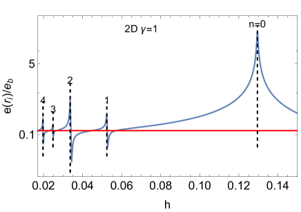
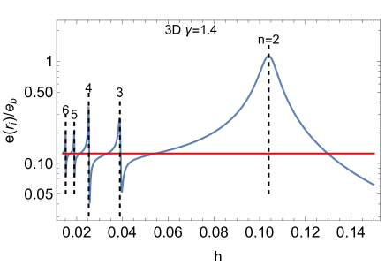
Figure 1: The forced eccentricity at the circumbinary disc inner edge ($r_{\rm i}=2a_{\rm b}$) normalized by the binary eccentricity is plotted on a log scale in blue as a function of disc aspect ratio $h$ for the 2D and 3D disc models described in Section 3. The forced eccentricity of a test particle at the same radius as the disc inner edge is plotted on the red line that is determined by $E_{\rm p}(r_{\rm i})$ in equation (6). Each black vertical dashed line occurs at an $h$ value for a free mode at zero frequency where a global resonance occurs. The number $n$ with each vertical line is the number of nodes in $E(r)$ for the free mode.

We now demonstrate that the peak eccentricities correspond to the values of $h$ for which a free eccentric mode has zero precession frequency. The driving of the eccentricity by the binary occurs at its apsidal precession frequency of zero. Therefore, the disc undergoes a global apsidal resonance at $h$ values (all other parameters being fixed) for which the free precession frequency equals the zero value of the driving frequency. To compute the free modes, we again solve equations (5) and (7) with $\partial_{t}E=0$ but with $\Phi_{\rm e}=0$ and without dissipation, $\alpha_{\rm b}=0$. We apply normalization condition $E(r_{\rm i})=1$, along with $\partial_{r}E=0$ at the inner and outer boundaries. Free modes with arbitrary values of $h$ generally have nonzero precession rates, so that $\partial_{t}E\neq 0$. We determine the values of $h$ for which $\partial_{t}E=0$, Some resulting zero frequency 2D and 3D free modes are plotted in Figure 2, There are infinitely many such modes that differ in the number of radial nodes $n$.

The $h$ values for the five lowest $n$ zero frequency free modes in the 2D and 3D models are plotted as dashed vertical lines in Figure 1. The plot shows that the $h$ values of the zero frequency modes occur at the forced eccentricity peaks in Figures 1. Therefore, we see that these peaks are a consequence of a resonance in which the zero frequency driving matches the zero frequency of a free mode in the disc. The peak forced eccentricity at a resonance approaches the test particle value with increasing $n$. We also find that the peak forced eccentricities vary with bulk viscosity as $\propto 1/\alpha_{\rm b}$, as would be expected for a resonant effect.

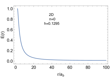
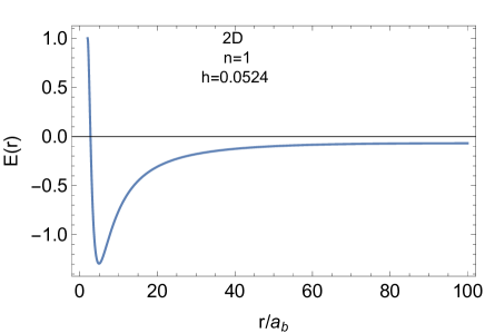
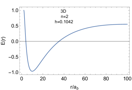
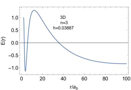
Figure 2: The eccentricity distribution for stationary (nonprecessing) free modes that occur for particular disc aspect ratios $h$ in the 2D and 3D disc models described in Section 3. The value of $n$ is the number of nodes. These modes are subject to a global resonance due to binary forcing.

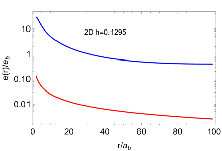
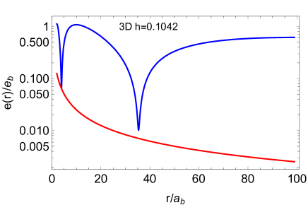
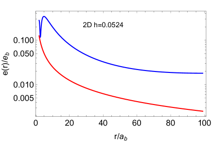
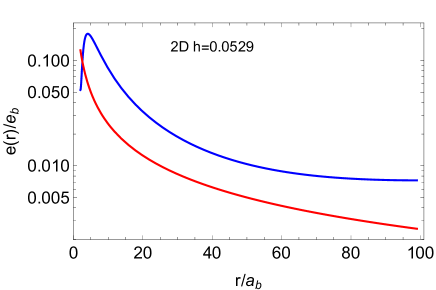
Figure 3: The magnitude of the forced eccentricity is plotted on a log scale as a function of radius for the disc (blue) and test particles (red). The plots are for parameters that are close to resonance.

Figure 3 plots in blue the magnitude of the forced eccentricity as a function of radius for the 2D and 3D discs with $h$ values that are close to resonance. Plotted in red is the forced eccentricity for test particles. The upper two panels show that shapes of the distributions reflect the distributions of the resonant free modes that have $n=0$ for the 2D case and $n=2$ for the 3D case, as plotted in Figure 2. The forced eccentricity distributions for the disc generally have much higher values than for test particles. For the 2D disc case at $h=0.1295$, the disc forced eccentricity distribution has a similar fall off in radius as the test particle case. In the 3D case the disc forced eccentricity distribution is much broader than in the test particle case.

The bottom two panels of Figure 3 illustrate why there are closely spaced local maximum and minimum values of $e(r_{\rm i})/e_{\rm b}$ near $h=0.0524$ for the 2D model in Figure 1. At this $h$ value, there is a zero frequency free mode as seen in Figure 2. In the third panel from the top of Figure 3, there are two local maxima for this $h$ value, while at a slightly higher value of $h$ shown in the bottom panel there is a single local maximum and a smaller value of forced eccentricity at the disc inner edge. The transition with decreasing $h$ from single to double maxima then occurs at a zero frequency resonance. This change is accompanied by a local minimum of $e(r_{\rm i})/e_{\rm b}$ as a function of $h$. This example explains why there are the pairs of closely spaced local maximum and minimum values seen in Figure 1. Near each resonance there is a change in the number of local maxima in the forced eccentricity distributions.

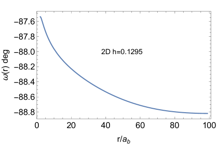
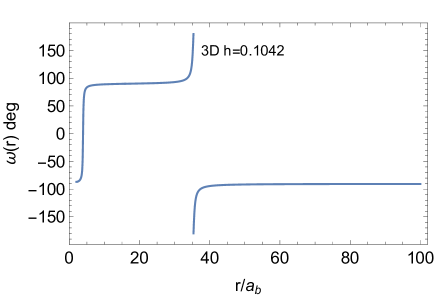
Figure 4: The phase of the disc forced eccentricity is plotted as a function of radius for 2D and 3D cases near resonance.

Figure 4 plots the phase of the forced eccentricity as a function of radius for the 2D and 3D cases with parameters that are close to resonance. In the plotted 2D case, which is for the $n=0$ mode, the phase is nearly independent of radius. The phase varies considerably in the 3D case that is plotted for the $n=2$ mode. The phase changes involves shifts by $180^{\circ}$ at forced eccentricity nodes that are broadened by viscosity. Otherwise the phase is fairly constant at $\simeq\pm 90^{\circ}$.

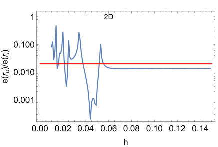
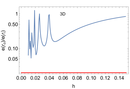
Figure 5: The ratio of forced eccentricity at the outer to inner edge of the circumbinary disc is plotted on a log scale in blue as a function of disc aspect ratio $h$ for the 2D and 3D disc models described in Section 3. The forced eccentricity ratio of test particles is plotted on the red line and is equal to 0.02.

Figure 5 plots in blue the ratio of the forced eccentricity at the outer to inner disc edge as a function of disc aspect ratio $h$ for the 2D and 3D cases. Plotted in red is this ratio for test particles. The plot crudely indicates the radial extent of the disc forced eccentricity. The plot provides another way to show that the distribution of disc forced eccentricity is very different from the test particle eccentricity distribution and is more different in 3D than 2D. We have checked that for very small $h<4\times 10^{-4}$ (not plotted) the disc and test particle ratios are nearly equal, as is expected in the small pressure limit. The structure of the plots is affected by the locations of the disc resonances evident as peaks in Figure 1. For the 2D case with $h\ga 0.06$, the disc eccentricity ratio is consistently smaller than the test particle ratio by about 30%. While in the 3D disc case with $h\ga 0.06$, the ratio is much larger, indicating that the 3D forced eccentricity distributions are much broader, as is evident in Figure 3. The forced eccentricity ratio is generally larger for the 3D disc case across all disc aspect ratios.

4 Existence of Zero Frequency Free Modes

The properties of the forced eccentricity are determined by resonances in the disc. Within the framework of the current model, such resonances rely on the existence of zero frequency free apsidal modes in the disc, as seen in Figure 1. In this section we discuss the conditions required for such modes to exist.

A useful measure of the effects of disc eccentricity is the angular momentum deficit

$$A_{\rm d}=\int_{r_{\rm i}}^{r_{\rm o}}\frac{1}{2}|E|^{2}\Sigma r^{2}\Omega 2\pi rdr$$ (8)

(Teyssandier & Ogilvie, 2016). This quantity measures the angular momentum difference of a slightly eccentric disc from a circular state with the same orbital energy. For the strongest resonance in 2D disc that has $h=0.1295$ and the 3D disc with $h=0.1042$ in Figure 1, the angular momentum deficits are $A_{\rm d}=0.93e_{\rm b}^{2}J_{\rm d}$ and $0.14e_{\rm b}^{2}J_{\rm d}$ respectively, where $J_{\rm d}$ is the disc angular momentum.

4.1 2D Modes

In this subsection we discuss how 2D free modes are able to satisfy the zero frequency condition required for resonance. By manipulating the equation (7), we calculate the frequency of free mode in terms of its eigenfunction $E(r)$ (Goodchild & Ogilvie, 2006). The frequency of a free mode can be decomposed as

$$\omega=\omega_{\rm g}+\omega_{\rm p1}+\omega_{\rm p2},$$ (9)

where

$$\omega_{\rm g} = -\frac{\pi}{2A_{\rm d}}\int^{r_{\rm o}}_{r_{\rm i}}\partial_{r}\left(r^{2}\partial_{r}\Phi_{\rm a}\right)|E(r)|^{2}\Sigma(r)rdr,$$ (10)

$$\omega_{\rm p1} = -\frac{\pi\gamma}{2A_{\rm d}}\int^{r_{\rm o}}_{r_{\rm i}}|\partial_{r}E(r)|^{2}Pr^{3}dr,$$ (11)

$$\ \omega_{\rm p2} = \frac{\pi}{2A_{\rm d}}\int^{r_{\rm o}}_{r_{\rm i}}|E(r)|^{2}\partial_{r}P\,r^{2}dr,$$ (12)

(13)

$A_{\rm d}$ is the angular momentum deficit defined in equation (8), $\omega_{\rm g}$ is due to the gravitational effects of the binary, and $\omega_{\rm p1}$ and $\omega_{\rm p2}$ are due to pressure effects. In particular, $\omega_{\rm p1}$ is due to a flux term, the third term on the RHS of equation (5).

Since the gravitational precession term $\omega_{\rm g}$ is positive, the pressure precession terms must sum to a negative value in order to have a zero frequency mode. Since both pressure terms are negative, this requirement is satisfied for all $n\geq 0$. In fact, we find that zero frequency free modes exist for all $n$ for suitable values of $h$.

4.2 3D Modes

The existence of zero frequency free modes in 3D is more complicated than in the 2D case. By manipulating the equation (7), we calculate the frequency of free mode in terms of its eigenfunction $E(r)$ (Teyssandier & Ogilvie, 2016). The frequency of a free mode can be decomposed as

$$\omega=\omega_{\rm g}+\omega_{\rm p1}+\omega_{\rm p2}+\omega_{\rm p3},$$ (14)

where

$$\omega_{\rm g} = -\frac{\pi}{2A_{\rm d}}\int^{r_{\rm o}}_{r_{\rm i}}\partial_{r}\left(r^{2}\partial_{r}\Phi_{\rm a}\right)|E(r)|^{2}\Sigma(r)rdr,$$ (15)

$$\omega_{\rm p1} = -\frac{\pi}{2A_{\rm d}}\left(2-\frac{1}{\gamma}\right)\int^{r_{\rm o}}_{r_{\rm i}}|\partial_{r}E(r)|^{2}Pr^{3}dr,$$ (16)

$$\omega_{\rm p2} = \frac{\pi}{2A_{\rm d}}\left(4-\frac{3}{\gamma}\right)\int^{r_{\rm o}}_{r_{\rm i}}|E(r)|^{2}\partial_{r}P\,r^{2}dr,$$ (17)

$$\omega_{\rm p3} = \frac{3\pi}{2A_{\rm d}}\left(1+\frac{1}{\gamma}\right)\int^{r_{\rm o}}_{r_{\rm i}}|E(r)|^{2}P\,rdr,$$ (18)

$A_{\rm d}$ is the angular momentum deficit defined in equation (8), $\omega_{\rm g}$ is due to the gravitational effects of the binary, and $\omega_{\rm pi}$ for $i=1,2,3$ are due to pressure effects. In particular, $\omega_{\rm p1}$ is due to a flux term, the fourth term on the RHS of equation (7). Frequencies $\omega_{\rm g}$, $\omega_{\rm p1}$, and $\omega_{\rm p2}$ are similar to their 2D counterparts in equations (10), (11), and (12), respectively, and are in fact equal for $\gamma=1$. Frequency $\omega_{\rm p3}$ is due to 3D effects. We have numerically verified that equation (14) is satisfied with $\omega=0$ to machine accuracy for the 3D zero frequency adiabatic free modes in this paper.

Since the gravitational precession term $\omega_{\rm g}$ is positive, the pressure precession terms must sum to a negative value in order to have a zero frequency mode. Pressure term is $\omega_{\rm p3}$ is the only positive pressure contribution. However, it is not always small. For $P\propto r^{-s}$, it follows that $\omega_{\rm p2}+\omega_{\rm p3}<0$ requires that $s>3(1+\gamma)/(-3+4\gamma)$. This is condition is typically not satisfied, as is the case for the parameters in this paper that have $s=1.5$ and $\gamma=1.4$. An overall negative pressure induced precession is possible due to term $\omega_{\rm p1}$. This term becomes more important for higher $n$ modes for which the radial derivatives of eccentricity become increasingly important.

For the model we have considered, the fundamental mode $n=0$, as well as $n=1$, have only positive eigenfrequencies for any reasonable value of $h<0.2$. This result is consistent with the findings of Miranda & Rafikov (2018) who computed eigenfrequencies (precession frequencies) of the fundamental free mode in a similar configuration and reported only positive values.

With the parameters in this paper, zero frequency modes exist for modes with $n\geq 2$ due to the negative contribution of $\omega_{\rm p1}$. This term becomes more important with increasing $n$. As a result, lower pressure and thus lower $h$ values are required to obtain a zero frequency mode. This effect explains why the resonant peaks in Figure 1 occur at smaller $h$ with increasing $n$. Figure 6 shows that $\omega_{\rm p1}+\omega_{\rm g}\sim 8.86\omega_{\rm p1}/n^{2}<0$ for zero frequency modes with large $n$. The other pressure contributions, $\omega_{\rm p2}+\omega_{\rm p3}$, become unimportant at large $n$.

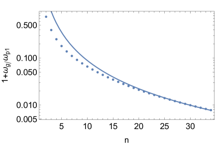
Figure 6: $1+\omega_{\rm g}/\omega_{\rm p1}$ plotted on a log scale against mode number $n\geq 2$ for zero frequency modes. The points plot the numerically determined values for each $n$. The disc aspect ratio decreases with increasing $n$. The solid line plots $8.86/n^{2}$.

5 Discussion

Mean motion resonances between perturber and a gas disc can play an important role in disc dynamics and eccentricity generation (Goldreich & Tremaine, 1979, 1980; Lubow, 1991). At such a resonance, the absolute value of the Doppler shifted frequency of a component of the forcing by the perturber matches the epicyclic frequency in the disc. In particular, the Lindblad resonances launch waves from a region that is of small radial extent (that scales with $h^{2/3}$) compared to the radius at the resonance. These waves then propagate and damp as they travel away from the resonance. The smallness of the wave generation region comes about because the frequency associated with such a mean motion resonance is high compared to frequency associated with the gas sound speed $c_{\rm s}/r$ for a thin disc. The radial width of the resonance depends then on the disc aspect ratio which is small. In the application of this resonance model to the case of secular forcing, the resonance radius would occur where the frequency of the secular forcing matches the apsidal precession frequency in the disc (Ward & Hahn, 1998). Since the strength of the Lindblad torque depends inversely on the frequency associated with a resonance, this model predicts that very strong torques are produced by the low frequency apsidal motions.

As pointed out by Goldreich & Sari (2003), the behavior of waves involving an apsidal resonance is quite different from the behavior in the mean motion resonance case. Because of their low frequency, apsidal waves are not generated in a small region of space. Instead such waves are better understood as global standing waves. Our results support that view. A similar situation occurs in the secular dynamics of tilted discs in binaries. Secular nodal resonances are also greatly broadened by gas pressure to the extent that the usual mean motion torques do not apply (Lubow & Ogilvie, 2001). The resonances we find here are global and occur for particular disc parameters, unlike the Lindblad resonances. Unlike the mean motion Lindblad resonance, this resonance does not provide a local site for wave launching. The disc forced eccentricity is affected by the resonance over the full radial extent of the mode.

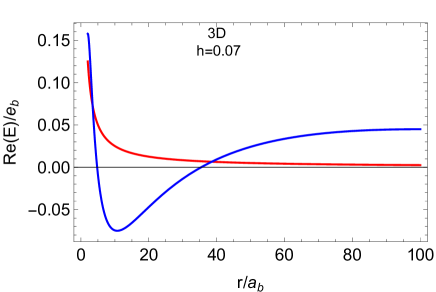
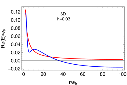
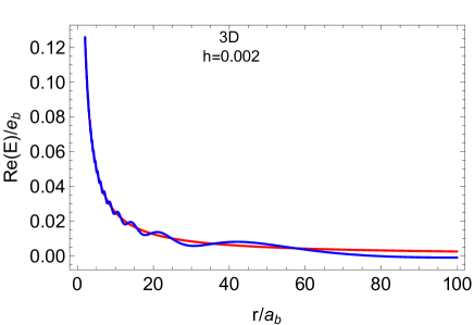
Figure 7: The real part of the forced eccentricity is plotted for the disc (blue) and test particles (red). The plots are for $h$ values that are between resonances. $Im(E)$ is much smaller in absolute value than $|Re(E)|$ and is not plotted.

The size of the inner cavity depends on binary eccentricity (Artymowicz & Lubow, 1994; Pelupessy & Portegies Zwart, 2013). If the size of the inner cavity is changed from our assumed value of $r_{\rm i}=2a_{\rm b}$, the resonances occur at different $h$ values from those in Figure 1. For example, if $r_{\rm i}$ is increased to $3a_{\rm b}$ , the $n=2$ resonance in the 3D case decreases from $h=0.10$ to 0.05. This is expected since the gravitational precession is weaker and so lower pressure is required for a zero frequency mode.

The torque associated with the forced eccentricity damping is given by

$$T=-\frac{\alpha_{\rm b}}{2}\int_{r_{\rm o}}^{r_{\rm o}}Pr^{2}\left|\frac{dE}{dr}\right|^{2}2\pi rdr$$ (20)

that is equal to the rate of change of angular momentum deficit for free waves given by equation (8) (Teyssandier & Ogilvie, 2016). This torque results in a binary eccentricity decrease and fixed semi-major axis. For the strongest resonance in 2D disc and the 3D disc plotted in Figure 1, $dln(e_{\rm b})/dt=-1.4\times 10^{-5}\,\Omega_{\rm b}J_{\rm d}/J_{\rm b}$ and $-1.7\times 10^{-7}\,\Omega_{\rm b}J_{\rm d}/J_{\rm b}$ respectively. for these two cases respectively. For example, for $\alpha_{\rm b}=0.01$ and $J_{\rm d}=0.1J_{\rm b}$, the timescale to change the binary eccentricity is about $1\times 10^{5}$ and $9\times 10^{6}$ binary orbital periods for these two cases. The results suggest that in the 3D case significant changes in binary eccentricity over a disc lifetime of $\sim 10^{6}$ yr can occur only if the binary period is fairly short, $<0.1$ yr. The timescale to change the binary eccentricity at resonance depends linearly on $\alpha_{\rm b}$. More complete calculations would take into account the effects of nonzero binary precession as a consequence of significant disc mass, as has been studied in the context of circumstellar discs by Silsbee & Rafikov (2015).

Simulations have been carried out that explore circumbinary disc eccentricity evolution involving eccentric orbit binaries (e.g., Miranda et al., 2017). Recently, Siwek et al. (2022) analyzed circumbinary disc eccentricity evolution using 2D simulations that covered a set of binary mass ratios and eccentricities. The results show disc eccentricity phase locking at large angles relative to the binary eccentricity, as we find here near resonances. On the other hand, phase locking of disc eccentricity was found in one case involving an equal mass eccentric orbit binary. Forced disc eccentricity does not occur for an equal mass binary that has $\mu=1/2$ (see equation (6)).

The forced eccentricity distributions that result for $h$ values between resonances in Figure 1 are strongly affected by the structure of the closest resonant modes, even when the disc forced eccentricity is not significantly amplified by a resonance. In the case of the 2D disc, the forced eccentricity distribution for $h>0.06$ resembles the fundamental mode (see Figure 2) due to the presence of the $n=0$ resonance. For smaller values of $h$ there are more complicated structures in the forced eccentricity distribution, due to effects of weak higher order resonances. For very small values of $h<0.005$, the disc forced eccentricity distribution approaches that of test particles.

The nonexistence of a resonance involving the fundamental mode in 3D, as discussed in Section 4.2, has interesting consequences. Consider for example $h=0.07$ that lies between the $h$ values of the $n=2$ and $n=3$ resonances shown in the bottom panel of Figure 1. In the top panel of Figure 7, we see that the forced eccentricity distribution resembles the $n=2$ free mode that is associated with the nearby resonance at $h=0.1042$ (see Figure 2), not the fundamental mode. This property holds for more generally for $h>0.045$. The value $h=0.03$ lies between the $n=3$ and $n=4$ resonances in the bottom panel of Figure 1. In the middle panel of Figure 7, we see that the forced eccentricity distribution is again not like the fundamental. For a much cooler disc with $h=0.002$ that lies between $h$ values for the $n=41$ and $n=42$ resonances, the forced eccentricity distribution is plotted in the bottom panel of Figure 7. There are wiggles resulting from the weak high $n$ resonances. The overall forced eccentricity distribution is similar that of test particles. For even cooler discs, the forced eccentricity distributions are indistinguishable from the test particle forced eccentricity distribution. Such cool discs may be relevant for the case involving supermassive black hole binaries.

On the other hand, the eccentricity distribution in an unforced 3D disc with some arbitrary initial eccentricity distribution would be expected to evolve over time to the fundamental mode distribution because higher $n$ modes are expected to decay faster (Miranda & Rafikov, 2018). However, we find that the situation is quite different for forced eccentricity in 3D, in which the fundamental mode distribution occurs only for very cool discs, $h<0.01$. More generally, which eccentric disc mode is excited also depends on the properties of the forcing. In the case of superhump binaries in which the circumstellar disc eccentricity is excited at the 3:1 resonance, the fastest growing disc mode depends on the disc outer radius and is not necessarily the fundamental (see Fig. 8 of Lubow, 2010).

6 Summary

We have analyzed the response of a gaseous circumbinary disc to secular forcing by an eccentric orbit central binary through the application of the disc eccentricity equations of Goodchild & Ogilvie (2006) and Teyssandier & Ogilvie (2016). The disc acquires a forced eccentricity that can significantly exceed the corresponding values for test particles (see Figures 1 and 3). The disc forced eccentricity is enhanced due to global apsidal resonances. The strongest enhancements occur for higher values of disc aspect ratios. At these resonances, the precession rate of a free disc mode matches the precession rate of the central binary that is zero in the case of a low mass disc. Due to the width of these resonances, the forced eccentricity is also enhanced for conditions near those for a resonance. Large phase shifts occur between the forced eccentricity of the disc and binary near resonance (Figure 4). The phase shifts sometimes vary in radius. The forced eccentricity distributions in 3D are typically broader than in the 2D case (Figure 5). Near each resonance there is a change in the number of local maxima in the forced eccentricity distributions (Figure 3).

For a disc not at resonance, the eccentricity distribution has somewhat similar form to the eccentricity distributions in discs at resonance that have the closest matching disc aspect ratios. For a 2D disc, the forced eccentricity distribution is similar to that of the fundamental mode over a broad range of parameters at higher disc aspect ratios $h>0.05$. In the case of a 3D disc, the forced eccentricity distribution is similar to that of higher order free modes, not the fundamental, unless the disc is very cool ($h<0.01$), as seen in Figure 7. This result is a consequence of the nonexistence of a zero frequency fundamental free mode in a 3D disc. For very cool discs, which may be of relevance to discs around supermassive black hole binaries, the nonresonant forced eccentricity distribution is similar to that of test particles, due to the low pressure.

The conditions required for resonance will change with parameter changes such as binary mass ratio and eccentricity, as well as the disc pressure variation in radius. At higher order, there is a dependence of potential $\Phi_{\rm a}$ in equation (1) on binary eccentricity that affects the conditions for resonance. In addition, the forcing potential $\Phi_{\rm e}$ in equation (2) varies with binary eccentricity beyond the lowest order linear approximation that we have adopted. For a disc of significant mass, the binary will undergo precession which in turn will modify the conditions required for resonance. Self-gravity could also modify the disc precession rate. In addition, the binary orbit might be modified by its secular interaction with the circumbinary disc. This study did not include the effects of shear viscosity that could play a role in causing additional phase shifts between the disc and binary. If high disc eccentricities are achieved, nonlinear dissipation though shocks may occur (e.g., Martin et al., 2014). While this paper has been concerned with circumbinary discs, similar resonance effects might occur with the secular eccentric forcing of circumstellar discs.

Data availability

The data underlying this article will be shared on reasonable request to the author.

References

- Artymowicz & Lubow (1994) Artymowicz P., Lubow S. H., 1994, ApJ, 421, 651
- Artymowicz & Lubow (1996) Artymowicz P., Lubow S. H., 1996, ApJl, 467, L77
- D’Orazio & Duffell (2021) D’Orazio D. J., Duffell P. C., 2021, ApJ, 914, L21
- D’Orazio et al. (2016) D’Orazio D. J., Haiman Z., Duffell P., MacFadyen A., Farris B., 2016, MNRAS, 459, 2379
- Dutrey et al. (2016) Dutrey A., Di Folco E., Beck T., Guilloteau S., 2016, A&ARv, 24, 5
- Farris et al. (2014) Farris B. D., Duffell P., MacFadyen A. I., Haiman Z., 2014, ApJ, 783, 134
- Goldreich & Sari (2003) Goldreich P., Sari R., 2003, ApJ, 585, 1024
- Goldreich & Tremaine (1979) Goldreich P., Tremaine S., 1979, ApJ, 233, 857
- Goldreich & Tremaine (1980) Goldreich P., Tremaine S., 1980, ApJ, 241, 425
- Goodchild & Ogilvie (2006) Goodchild S., Ogilvie G., 2006, MNRAS, 368, 1123
- Günther & Kley (2002) Günther R., Kley W., 2002, A&A, 387, 550
- Gutiérrez et al. (2022) Gutiérrez E. M., Combi L., Noble S. C., Campanelli M., Krolik J. H., López Armengol F., García F., 2022, ApJ, 928, 137
- Heath & Nixon (2020) Heath R. M., Nixon C. J., 2020, A&A, 641, A64
- Leung & Lee (2013) Leung G. C. K., Lee M. H., 2013, ApJ, 763, 107
- Lubow (1991) Lubow S. H., 1991, ApJ, 381, 259
- Lubow (2010) Lubow S. H., 2010, MNRAS, 406, 2777
- Lubow & Ogilvie (2001) Lubow S. H., Ogilvie G. I., 2001, ApJ, 560, 997
- MacFadyen & Milosavljević (2008) MacFadyen A. I., Milosavljević M., 2008, ApJ, 672, 83
- Martin et al. (2014) Martin R. G., Nixon C., Lubow S. H., Armitage P. J., Price D. J., Doğan S., King A., 2014, ApJL, 792, L33
- Marzari et al. (2013) Marzari F., Thebault P., Scholl H., Picogna G., Baruteau C., 2013, A&A, 553, A71
- Miranda & Rafikov (2018) Miranda R., Rafikov R. R., 2018, ApJ, 857, 135
- Miranda et al. (2017) Miranda R., Muñoz D. J., Lai D., 2017, MNRAS, 466, 1170
- Moriwaki & Nakagawa (2004) Moriwaki K., Nakagawa Y., 2004, ApJ, 609, 1065
- Muñoz & Lai (2016) Muñoz D. J., Lai D., 2016, ApJ, 827, 43
- Muñoz & Lithwick (2020) Muñoz D. J., Lithwick Y., 2020, ApJ, 905, 106
- Muñoz et al. (2019) Muñoz D. J., Miranda R., Lai D., 2019, ApJ, 871, 84
- Okazaki et al. (2002) Okazaki A. T., Bate M. R., Ogilvie G. I., Pringle J. E., 2002, MNRAS, 337, 967
- Paardekooper et al. (2008) Paardekooper S. J., Thébault P., Mellema G., 2008, MNRAS, 386, 973
- Pelupessy & Portegies Zwart (2013) Pelupessy F. I., Portegies Zwart S., 2013, MNRAS, 429, 895
- Shi et al. (2012) Shi J.-M., Krolik J. H., Lubow S. H., Hawley J. F., 2012, ApJ, 749, 118
- Silsbee & Rafikov (2015) Silsbee K., Rafikov R. R., 2015, ApJ, 798, 71
- Silsbee & Rafikov (2021) Silsbee K., Rafikov R. R., 2021, A&A, 652, A104
- Siwek et al. (2022) Siwek M., Weinberger R., Munoz D., Hernquist L., 2022, arXiv e-prints, p. arXiv:2203.02514