Interim Monitoring of Sequential Multiple Assignment Randomized Trials Using Partial Information

Abstract

The sequential multiple assignment randomized trial (SMART) is the gold standard trial design to generate data for the evaluation of multi-stage treatment regimes. As with conventional (single-stage) randomized clinical trials, interim monitoring allows early stopping; however, there are few methods for principled interim analysis in SMARTs. Because SMARTs involve multiple stages of treatment, a key challenge is that not all enrolled participants will have progressed through all treatment stages at the time of an interim analysis. Wu et al., (2021) propose basing interim analyses on an estimator for the mean outcome under a given regime that uses data only from participants who have completed all treatment stages. We propose an estimator for the mean outcome under a given regime that gains efficiency by using partial information from enrolled participants regardless of their progression through treatment stages. Using the asymptotic distribution of this estimator, we derive associated Pocock and O’Brien-Fleming testing procedures for early stopping. In simulation experiments, the estimator controls type I error and achieves nominal power while reducing expected sample size relative to the method of Wu et al., (2021). We present an illustrative application of the proposed estimator based on a recent SMART evaluating behavioral pain interventions for breast cancer patients.

Keywords: Augmented inverse probability weighting; Clinical trials; Double robustness; Dynamic treatment regimes; Early stopping; Group sequential analysis.

1 Introduction

Treatment of chronic diseases and disorders involves a series of treatment decisions made at critical points in the progression of a patient’s health status. To optimize long-term health outcomes, these decisions must adapt to evolving patient information, including response to previous treatments. Strategies for adapting treatment decisions over time are formalized as treatment regimes, which comprise a sequence of decision rules, one per stage of intervention, that map accrued patient information to a recommended treatment (Chakraborty and Moodie,, 2013; Tsiatis et al.,, 2020). The value of a regime is the expected utility if the regime is used to select treatments in the population of interest. A regime is optimal if it has maximal value. Much of the statistical literature on treatment regimes has focused on estimation and inference for optimal regimes (Kosorok and Laber,, 2019). However, scientific interest often focuses on comparison of a small number of pre-specified treatment regimes, either with each other or against a control, on the basis of mean outcome.

The gold standard for data collection for the evaluation of treatment regimes is the sequential multiple assignment randomized trial (SMART; Lavori and Dawson,, 2004; Murphy,, 2005). A SMART contains multiple stages of randomization, with each stage corresponding to a key decision point. In a SMART, if, when, and to whom a treatment might be randomly assigned is allowed to depend on a patient’s treatment and outcome history, leading to a rich and flexible class of designs. In the past decade, the use of SMARTs has increased dramatically; SMARTs have been conducted in a range of disease and disorder areas, including cancer (Wang et al.,, 2012; Thall,, 2015; Kelleher et al.,, 2017), behavioral sciences (Almirall et al.,, 2014; Kidwell and Hyde,, 2016), and mental health (Manschreck and Boshes,, 2007; Sinyor et al.,, 2010). For a comprehensive list of SMARTs, see Bigirumurame et al., (2022).

Every SMART can be equivalently represented as randomizing subjects at baseline among a set of fixed regimes known as the trial’s “embedded regimes.” Primary analyses in a SMART often focus on comparisons of the embedded regimes against each other or a control (Lavori and Dawson,, 2004; Murphy,, 2005). These comparisons are often used for sizing a SMART (Seewald et al.,, 2020; Artman et al.,, 2020). For example, Figure 1 shows a two-stage SMART schema for behavioral interventions for pain management in cancer patients with eight embedded regimes (Kelleher et al.,, 2017; ClinicalTrials.gov,, 2021). Each embedded regime takes the form “give intervention $a$; if response, give $b$; if non-response, give $c$;” e.g., give pain coping skills training (PCST) Full initially; if response, give maintenance; otherwise, give PCST-Plus. We discuss this study further in Section 7.

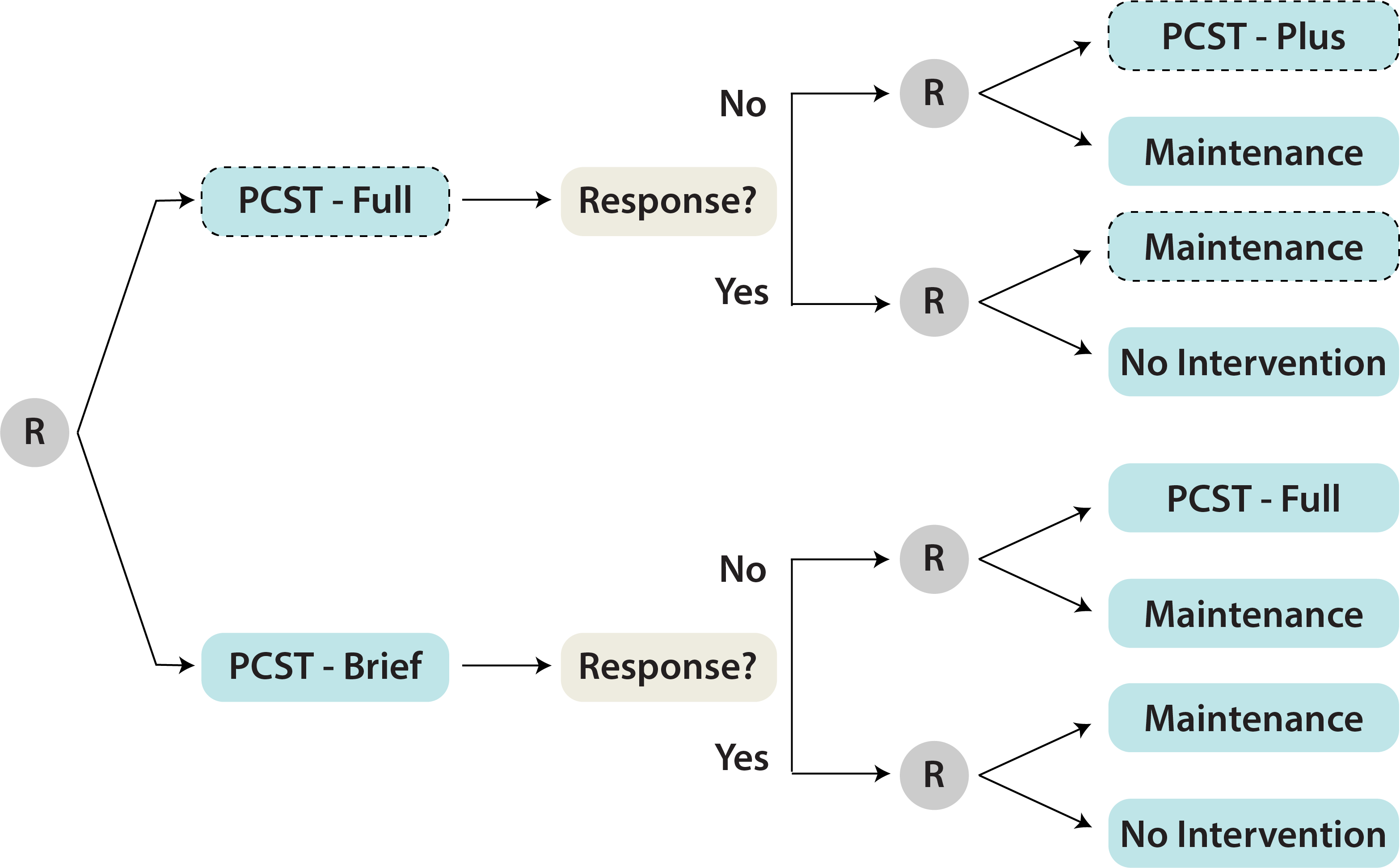
Figure 1: Schema for the SMART evaluating regimes involving behavioral interventions for pain management in breast cancer patients embedding eight regimes of the form “Give intervention $a$; if non-response, give $b$; otherwise, if response give $c$.” The embedded regime determined by $a$ = PCST-Full, $b$= PCST-Plus, $c$ = Maintenance is shown with dashed lines around the treatments. Regimes $l=1,\ldots,8$ take $(a,b,c)$ to be (Full, Plus, Maintenance), (Full, Plus, No Intervention), (Full, Maintenance, Maintenance), (Full, Maintenance, No Intervention), (Brief, Full, Maintenance), (Brief, Full, No Intervention), (Brief, Maintenance, Maintenance), and (Brief, Maintenance, No Intervention), respectively. This figure appears in color in the electronic version of this article.

Interim monitoring allows early stopping for efficacy or futility, which can reduce cost and accelerate evaluation of candidate treatments. Group sequential methods allowing early stopping are well established for conventional clinical trials (Jennison and Turnbull,, 2000). However, analogous methodology for SMARTs is limited. Wu et al., (2021) propose an interim test for a difference in mean outcome among embedded regimes in two-stage SMARTs. However, their approach is based on the inverse probability weighted estimator (IPWE), which does not incorporate baseline and accruing patient information that could be used to enhance efficiency (Zhang et al.,, 2013). Chao et al., (2020) consider interim analysis for a small-$n$, two-stage SMART restricted to the specific situation in which the same treatments are available at each stage and the goal is to remove futile treatments.

We develop a class of interim analysis methods for SMARTs based on an augmented inverse probability weighted estimator (AIPWE) for the value of a regime that increases statistical efficiency by using partial information from individuals with incomplete regime trajectories. Our method applies to SMARTs with an arbitrary number of stages and treatments, as well as those in which the set of allowable treatments depends on a patient’s history. We present the statistical framework in Section 2. In Section 3, we review the AIPWE for the value of a regime when all participants have progressed through all stages. We introduce the proposed Interim AIPWE in Section 4. In Section 5, we discuss testing procedures, stopping boundaries, and sample size formulæ for interim analysis. In Section 6, we evaluate the empirical performance of the proposed procedure in a series of simulation experiments, and we present a case study based on the cancer pain management SMART in Section 7.

2 Statistical framework

Consider a SMART with $K$ stages and a planned total sample size of $N$. Each subject completing the trial generates a trajectory of the form $(\mathbf{X}_{1},A_{1},\mathbf{X}_{2},A_{2},\dots,\mathbf{X}_{K},A_{K},Y)$, where $A_{k}\in\mathcal{A}_{k}$, $k=1,\ldots,K$, is the treatment assigned at stage $k$; $\mathcal{A}_{k}$ is a finite set of treatment options at decision $k$; $\mathbf{X}_{1}\in\mathbb{R}^{p_{1}}$ comprises baseline subject variables; $\mathbf{X}_{k}\in\mathbb{R}^{p_{k}}$, $k=2,\ldots,K$, comprises subject variables collected between stages $k-1$ and $k$; and $Y\in\mathbb{R}$ is an outcome measured at the end of follow up, coded so that higher values are better. Let $\overline{\mathbf{X}}_{k}=(\mathbf{X}_{1},\ldots,\mathbf{X}_{k})$ and $\overline{\mathbf{A}}_{k}=(A_{1},\ldots,A_{k})$, and define $\mathbf{H}_{1}=\mathbf{X}_{1}$ and $\mathbf{H}_{k}=(\overline{\mathbf{X}}_{k},\overline{\mathbf{A}}_{k-1})$, $k\geq 2$, so that $\mathbf{H}_{k}$ is the information available at the time $A_{k}$ is assigned. Let $\mathcal{H}_{k}=\mathrm{dom}\ \mathbf{H}_{k}$ and let $2^{\mathcal{A}_{k}}$ denote the power set of $\mathcal{A}_{k}$. We assume there exists a set-valued function $\Psi_{k}:\mathcal{H}_{k}\rightarrow 2^{\mathcal{A}_{k}}$ so that the set of allowable treatments for a subject with $\mathbf{H}_{k}=\mathbf{h}_{k}$ at stage $k$ is $\Psi_{k}(\mathbf{h}_{k})\subseteq\mathcal{A}_{k}$ (van der Laan and Petersen,, 2007; Tsiatis et al.,, 2020).

In this setting, a treatment regime is a sequence of decision rules, $\mathbf{d}=(d_{1},\ldots,d_{K})$, where $d_{k}:\mathcal{H}_{k}\to\mathcal{A}_{k}$ and $d_{k}(\mathbf{h}_{k})\in\Psi_{k}(\mathbf{h}_{k})$ for all $\mathbf{h}_{k}\in\mathcal{H}_{k}$, $k=1,\ldots,K$. Let $Y^{*}(\overline{\mathbf{a}}_{K})$ denote the potential outcome under treatment sequence $\overline{\mathbf{a}}_{K}=(a_{1},\ldots,a_{K})$, and let $\mathbf{X}_{k}^{*}(\overline{\mathbf{a}}_{k-1})$ denote the potential intermediate variables under sequence $\overline{\mathbf{a}}_{k-1}$ at stage $k\geq 2$. Define $\overline{\mathbf{X}}^{*}_{k}(\overline{\mathbf{a}}_{k-1})=\{\mathbf{X}_{1},\mathbf{X}^{*}_{2}(a_{1}),\ldots,\mathbf{X}^{*}_{k}(\overline{\mathbf{a}}_{k-1})\}$, $\mathbf{H}_{k}^{*}(\overline{\mathbf{a}}_{k-1})=\{\overline{\mathbf{X}}^{*}_{k}(\overline{\mathbf{a}}_{k-1}),\overline{\mathbf{a}}_{k-1}\}$, and $\mathbf{H}_{1}^{*}(a_{0})=\mathbf{H}_{1}$. The potential covariates and outcome for an individual receiving treatment according to regime $\mathbf{d}$ are

$$\mathbf{X}^{*}_{k}(\mathbf{d}) =\sum_{\overline{\mathbf{a}}_{k-1}\in\mathcal{A}_{1}\times\cdots\times\mathcal{A}_{k-1}}\mathbf{X}^{*}(\overline{\mathbf{a}}_{k-1})\prod_{k=1}^{k-1}I\left[a_{k}=d_{k}\left\{\mathbf{H}_{k}^{*}(\overline{\mathbf{a}}_{k-1})\right\}\right],k=2,\ldots,K,$$

$$Y^{*}(\mathbf{d}) =\sum_{\overline{\mathbf{a}}_{K}\in\mathcal{A}_{1}\times\cdots\times\mathcal{A}_{K}}Y^{*}(\overline{\mathbf{a}}_{K})\prod_{k=1}^{K}I\left[a_{k}=d_{k}\left\{\mathbf{H}_{k}^{*}(\overline{\mathbf{a}}_{k-1})\right\}\right].$$

The mean outcome, or value, for a regime $\mathbf{d}$ is $V(\mathbf{d})=\mathbb{E}\{Y^{*}(\mathbf{d})\}$.

In a SMART, primary analyses often focus on inference on $V(\mathbf{d})$ for regimes $\mathbf{d}$ that are embedded in the trial. Let $\pi_{k}(a_{k},\mathbf{h}_{k})=P(A_{k}=a_{k}|\mathbf{H}_{k}=\mathbf{h}_{k})$ be the probability (propensity) of being randomized to treatment $a_{k}\in\Psi_{k}(\mathbf{h}_{k})$ at stage $k$ for a subject with history $\mathbf{h}_{k}$. It is well known that $V(\mathbf{d})$ is identifiable under the following conditions: positivity ($\pi_{k}(a_{k},\mathbf{h}_{k})>0$ for all $\mathbf{h}_{k}\in\mathcal{H}_{k}$ and $a_{k}\in\Psi_{k}(\mathbf{h}_{k})$); sequential randomization ($\{\mathbf{X}_{1},\mathbf{X}^{*}_{2}(a_{1}),\ldots,\mathbf{X}^{*}_{k}(\overline{\mathbf{a}}_{k-1}),Y^{*}(\overline{\mathbf{a}}_{K})\}_{\overline{\mathbf{a}}_{K}\in\mathcal{A}_{1}\times\cdots\times\mathcal{A}_{K}}\perp\!\!\!\perp A_{k}|\mathbf{H}_{k}$ at each stage $k$ for all $\overline{\mathbf{a}}_{K}$, where $\perp\!\!\!\perp$ denotes independence), which holds by design in a SMART; consistency, $Y=Y^{*}(\overline{\mathbf{A}}_{K})$ and $\mathbf{H}_{k}=\mathbf{H}_{k}^{*}(\overline{\mathbf{A}}_{k-1})$; and no interference among subjects (Tsiatis et al.,, 2020). Hereafter, we assume that these conditions hold.

Take $\mathbf{d}^{\ell}$, $\ell=1,\ldots,L$, to be the regimes embedded in the SMART and $\mathbf{d}^{0}$ a possible control, e.g., a treatment or regime representing the standard of care. For definiteness, we consider two null hypotheses that address the efficacy of the embedded regimes:

Homogeneity $$H_{0H}:V(\mathbf{d}^{1})=\cdots=V(\mathbf{d}^{L})$$ (1)

Superiority $$H_{0D}:V(\mathbf{d}^{\ell})-V(\mathbf{d}^{0})\leq\delta\text{ for all }\ell=1,\ldots,L.$$ (2)

These hypotheses are analogous to those used in multi-arm, multi-stage and platform trials (Jennison and Turnbull,, 2000, Chapter 16; Wason,, 2019). The control value $V(\mathbf{d}^{0})$ may be fixed or estimated from an additional control arm. The methods presented here apply to futility testing with minor modification. Hypotheses that stop the trial for either a single regime or all regimes falling below an efficacy boundary are possible in this construction.

3 AIPWE for complete data

We briefly review the AIPWE of the value in the setting where one observes $N$ complete independent and identically distributed trajectories $\left\{\mathbf{X}_{1,i},A_{1,i},\ldots,\mathbf{X}_{K,i},A_{K,i},Y_{i}\right\}_{i=1}^{N}$. For any regime $\mathbf{d}$, define $\mathcal{C}_{\mathbf{d},k}=\prod_{j=1}^{k}I\left\{A_{j}=d_{j}(\mathbf{H}_{j})\right\}$ to be an indicator that treatment is consistent with $\mathbf{d}$ through the first $k$ decisions, and let $\mathcal{C}_{\mathbf{d},0}=1$. For each $k=1,\ldots,K$, let $\pi_{k}(a_{k},\mathbf{h}_{k};\boldsymbol{\theta}_{k})$ be a posited model for $\pi_{k}(a_{k},\mathbf{h}_{k})$ indexed by $\boldsymbol{\theta}_{k}\in\boldsymbol{\Theta}_{k}$. Although the propensities are known in a SMART, estimating them based on correctly specified models can increase efficiency (Tsiatis, 2006b, ). Let $\widehat{\boldsymbol{\theta}}_{k,N}$ be an estimator of $\boldsymbol{\theta}_{k}$. The form of the AIPWE for $V(\mathbf{d})$ is (Zhang et al.,, 2013; Tsiatis et al.,, 2020, Section 6.4.4)

$$\widehat{V}_{\mathrm{A}}(\mathbf{d})=N^{-1}\sum_{i=1}^{N}\Bigg{[}\frac{Y_{i}\ \mathcal{C}_{\mathbf{d},K,i}}{\prod_{k=1}^{K}\pi_{k}(A_{k,i},\mathbf{H}_{k,i};\widehat{\boldsymbol{\theta}}_{k,N})}\\ +\sum_{k=1}^{K}\left\{\frac{\mathcal{C}_{\mathbf{d},k-1,i}}{\prod_{v=1}^{k-1}{\pi}_{v}(A_{v,i},\mathbf{H}_{v,i};\widehat{\boldsymbol{\theta}}_{v,N})}-\frac{\mathcal{C}_{\mathbf{d},k,i}}{\prod_{v=1}^{k}{\pi}_{v}(A_{v,i},\mathbf{H}_{v,i};\widehat{\boldsymbol{\theta}}_{v,N})}\right\}L_{k}(\overline{\mathbf{X}}_{ki})\Bigg{]},$$ (3)

where $L_{k}(\overline{\mathbf{x}}_{k})$ is an arbitrary function of $\overline{\mathbf{x}}_{k}$ and we define $\prod_{v=1}^{0}{\pi}_{v}(A_{v,i},\mathbf{H}_{v,i};\widehat{\boldsymbol{\theta}}_{v,N})=1$. Setting $L_{k}(\overline{\mathbf{x}}_{k})\equiv 0$ yields the IPWE that forms the basis for the approach of Wu et al., (2021); the IPWE uses only the observed outcomes and no covariate information. It can be an inefficient estimator for $V(\mathbf{d})$ when there are covariates that are correlated with the outcome. The efficient choice for $L_{k}$ is $L_{k}^{\mathbf{d}}(\overline{\mathbf{x}}_{k})=E\{Y^{*}(\mathbf{d})|\overline{\mathbf{X}}_{k}=\overline{\mathbf{x}}_{k},\overline{\mathbf{A}}_{k-1}=\overline{\mathbf{d}}_{k-1}(\overline{\mathbf{x}}_{k-1})\}$, where $\overline{\mathbf{d}}_{k}(\overline{\mathbf{x}}_{k})$ is defined as follows: $\overline{d}_{1}(\mathbf{x}_{1})=d_{1}(\mathbf{x}_{1})$, $\overline{\mathbf{d}}_{2}(\overline{\mathbf{x}}_{2})=[d_{1}(\mathbf{x}_{1}),d_{2}\{\overline{\mathbf{x}}_{2},d_{1}(\mathbf{x}_{1})\}],\ldots,\overline{\mathbf{d}}_{k}(\overline{\mathbf{x}}_{k})=[d_{1}(\mathbf{x}_{1}),d_{2}\{\overline{\mathbf{x}}_{2},d_{1}(\mathbf{x}_{1})\},\ldots,d_{k}\{\overline{\mathbf{x}}_{k},\overline{\mathbf{d}}_{k-1}(\overline{\mathbf{x}}_{k-1})\}]$, $k=1,\ldots,K$; and $\overline{\mathbf{A}}_{k}=\overline{\mathbf{d}}_{k}(\overline{\mathbf{X}}_{k})$ is the event that all treatments received are consistent with $\mathbf{d}$ through decision $k$.

In practice, the functions $L_{k}^{\mathbf{d}}(\overline{\mathbf{x}}_{k}),\,k=1,\ldots,K$ are unknown, but they can be estimated using $Q$-learning as follows (Tsiatis et al.,, 2020, Section 6.4.2). Posit a model $Q_{K}(\overline{\mathbf{x}}_{K},\overline{\mathbf{a}}_{K};\boldsymbol{\beta}_{K})$ for $Q_{K}(\overline{\mathbf{x}}_{K},\overline{\mathbf{a}}_{K})=\mathbb{E}(Y|\overline{\mathbf{X}}_{K}=\overline{\mathbf{x}},\overline{\mathbf{A}}_{K}=\overline{\mathbf{a}}_{K})$ indexed by $\boldsymbol{\beta}_{K}\in\mathcal{B}_{K}\subseteq\mathbb{R}^{P_{Q_{K}}}$. Obtain an estimator $\widehat{\boldsymbol{\beta}}_{K,N}$ for $\boldsymbol{\beta}_{K}$ by an appropriate regression method, e.g., least squares, and take $\widehat{L}_{K}^{\mathbf{d}}(\overline{\mathbf{x}}_{K})=Q_{K}\{\overline{\mathbf{x}}_{K},\overline{\mathbf{d}}_{K}(\overline{\mathbf{x}}_{K});\widehat{\boldsymbol{\beta}}_{K,N}\}$. Define the pseudo-outcomes at stage $k=K-1,\ldots,1$ as $Q_{k+1}^{\mathbf{d}}[\overline{\mathbf{X}}_{k+1,i},\left\{\overline{\mathbf{A}}_{k,i},d_{k+1}(\overline{\mathbf{X}}_{k+1,i},\overline{\mathbf{A}}_{k,i})\right\};\widehat{\boldsymbol{\beta}}_{k+1,N}]$, the predicted outcome using the fitted model when individuals receive consistent treatments at stage $k+1$. Then, obtain $\widehat{\boldsymbol{\beta}}_{k,N}^{\mathbf{d}}$ by a suitable regression method using the pseudo-outcomes as the response, e.g., for least squares,

$$\widehat{\boldsymbol{\beta}}_{k,N}^{\mathbf{d}}=\arg\min_{\boldsymbol{\beta}_{k}}\sum_{i=1}^{n}\left\{Q_{k+1}^{\mathbf{d}}\left[\overline{\mathbf{X}}_{k+1,i},\left\{\overline{\mathbf{A}}_{k,i},d_{k+1}(\overline{\mathbf{X}}_{k+1,i},\overline{\mathbf{A}}_{k,i})\right\};\widehat{\boldsymbol{\beta}}_{k+1,N}\right]-Q_{k}^{\mathbf{d}}\left(\overline{\mathbf{X}}_{k},\overline{\mathbf{A}}_{k};\boldsymbol{\beta}_{k}\right)\right\}^{2},$$

and $\widehat{L}^{\mathbf{d}}_{k}(\overline{\mathbf{x}}_{k})=Q^{\mathbf{d}}_{k}\{\overline{\mathbf{x}}_{k},\overline{\mathbf{d}}_{k}(\overline{\mathbf{x}}_{k});\widehat{\boldsymbol{\beta}}_{k,N}\}$. For individuals with only one treatment available at stages $k$ to $k^{\prime}$, we use pseudo-outcome $Q_{k^{\prime}+1}^{\mathbf{d}}[\overline{\mathbf{X}}_{k^{\prime}+1,i},\left\{\overline{\mathbf{A}}_{k^{\prime},i},d_{k^{\prime}+1}(\overline{\mathbf{X}}_{k^{\prime}+1,i},\overline{\mathbf{A}}_{k^{\prime},i})\right\};\widehat{\boldsymbol{\beta}}_{k^{\prime}+1,N}]$ for $k^{\prime}<K-1$ and $Y$ for $k^{\prime}=K-1$ (Tsiatis et al.,, 2020, Section 6.4.2).

The estimator (3) is doubly robust, i.e., it consistently estimates $V(\mathbf{d})$ if either of the sets of models $\pi_{k}(a_{k},\mathbf{h}_{k};\boldsymbol{\theta}_{k})$, $k=1,\ldots,K$, or $Q_{K}(\overline{\mathbf{x}}_{K},\overline{\mathbf{a}}_{K};\boldsymbol{\beta}_{K})$, $Q_{k}^{\mathbf{d}}(\overline{\mathbf{x}}_{k},\overline{\mathbf{a}}_{k};\boldsymbol{\beta}_{k})$, $k=1,\ldots,K$, is correctly specified (Han,, 2014; Vermeulen and Vansteelandt,, 2015; Luedtke et al.,, 2018; Tsiatis et al.,, 2020). Consistency is guaranteed in SMARTs because propensities are known.

4 Interim AIPW estimator

The interim AIPW estimator (IAIPWE) uses partial information from individuals who have yet to complete follow up at the times interim analyses are conducted; the IAIPWE includes the IPWE and AIPWE for complete data as special cases. Assume that the enrollment process is independent of all subject information and that the time between stages is fixed, as is the case for many SMARTs. Let $S$ be the number of planned analyses. Let $\Gamma(t)\in\{0,1\}$ be an indicator that a participant has enrolled in the SMART at study time $t$, where $t=0$ denotes the start of the study (in calendar time). In addition, let $\kappa(t)\in\left\{0,1,\ldots,K\right\}$ be the furthest stage reached by a participant at time $t$ with $\Gamma(t)=0\Rightarrow\kappa(t)=0$; and let $\Delta(t)\in\{0,1\}$ be an indicator that a participant has completed follow up, i.e., they have completed all $K$ stages and have had their outcome ascertained. Thus, the number of participants enrolled at time $t$ is $n(t)=\sum_{i=1}^{N}\Gamma_{i}(t)$. We evaluate either the fixed set of $L$ embedded regimes $\left\{\mathbf{d}^{\ell}\right\}_{\ell=1}^{L}$ for null hypothesis (1), or the embedded regimes along with a control regime, $\mathbf{d}^{0}$, for null hypothesis (2). The control regime may be estimated from a separate trial arm or may have a predetermined fixed value. We use superscript $\ell$ to indicate that a quantity is being computed for regime $\mathbf{d}^{\ell}$, e.g., $\widehat{\boldsymbol{\beta}}_{k,N}^{\ell}$ is shorthand for $\widehat{\boldsymbol{\beta}}_{k,N}^{\mathbf{d}^{\ell}}$.

We define the “full data” under regime $\mathbf{d}^{\ell}$ as $W^{*}_{\mathbf{d}^{\ell}}=\{Y^{*}(\mathbf{d}^{\ell}),\overline{\mathbf{X}}_{K}^{*}(\mathbf{d}^{\ell})\}$, which comprises the potential outcome $Y^{*}(\mathbf{d}^{\ell})$ and associated potential covariates $\overline{\mathbf{X}}_{K}^{*}(\mathbf{d}^{\ell})=\{\mathbf{X}_{1},\mathbf{X}^{*}_{2}(\mathbf{d}^{\ell}),\ldots,\\ \mathbf{X}^{*}_{k}(\mathbf{d}^{\ell})\}$. The observed data for an individual at time $t$ are therefore $W(t)=\Gamma(t)\big{[}1,\ \kappa(t),\ \mathbf{X}_{1},\ \\ A_{1},\ I\{\kappa(t)>1\}\mathbf{X}_{2},\ I\{\kappa(t)>1\}A_{2},\ \ldots\ ,\ I\{\kappa(t)>K-1\}\mathbf{X}_{K},\ I\{\kappa(t)>K-1\}A_{K},\ \Delta(t),\ \\ \Delta(t)Y\big{]}.$ For a given time $t$ and regime $\mathbf{d}^{\ell}$, let $\mathcal{R}^{\ell}(t)\in\left\{1,\ldots,2K,\infty\right\}$ be a discrete coarsening variable, which is defined as follows:

$$\mathcal{R}^{\ell}(t)=1 \quad A_{1}\neq d_{1}^{\ell}(\mathbf{H}_{1})$$ if

$$\mathcal{R}^{\ell}(t)=2 \quad\mathcal{C}_{\mathbf{d}^{\ell},{1}}=1,\kappa(t)=1$$ if

$$\mathcal{R}^{\ell}(t)=3 \quad\mathcal{C}_{\mathbf{d}^{\ell},{1}}=1,\kappa(t)=2,A_{2}\neq d_{2}^{\ell}(\mathbf{H}_{2})$$ if

$$\mathcal{R}^{\ell}(t)=4 \quad\mathcal{C}_{\mathbf{d}^{\ell},{2}}=1,\kappa(t)=2$$ if

$$\quad\vdots$$

$$\mathcal{R}^{\ell}(t)=2k-1 \quad\mathcal{C}_{\mathbf{d}^{\ell},{k-1}}=1,\kappa(t)=k,A_{k}\neq d_{k}^{\ell}(\mathbf{H}_{k})$$ if

$$\mathcal{R}^{\ell}(t)=2k \quad\mathcal{C}_{\mathbf{d}^{\ell},k}=1,\kappa(t)=k$$ if

$$\quad\vdots$$

$$\mathcal{R}^{\ell}(t)=2K \quad\mathcal{C}_{\mathbf{d}^{\ell},{K}}=1,\kappa(t)=K,\Delta(t)\neq 1$$ if

$$\mathcal{R}^{\ell}(t)=\infty \quad\mathcal{C}_{\mathbf{d}^{\ell},{K}}=1,\kappa(t)=K,\Delta(t)=1.$$ if

Thus, $\mathcal{R}^{\ell}(t)=\infty$ corresponds to a participant having completed follow up and being consistent with $\mathbf{d}^{\ell}$ for all treatment decisions at time $t$. For $\mathcal{R}^{\ell}(t)<\infty$, $\lfloor\mathcal{R}^{\ell}(t)/2\rfloor$ is the number of stages at which a participant is consistent with $\mathbf{d}^{\ell}$ at time $t$, and $\mathcal{R}^{\ell}(t)\mod 2$ encodes whether the number of consistent stages is due to time-related censoring, i.e., not having yet completed the current stage, or having been assigned a treatment that is inconsistent with $\mathbf{d}^{\ell}$. See Appendix A for an example of how $\mathcal{R}^{\ell}(t)$ is determined.

The observed data $W(t)$ are a coarsened version of the full data $W^{*}_{\mathbf{d}^{\ell}}$. The coarsening is monotone in that the full data coarsened to level $\mathcal{R}^{\ell}(t)=r$ are a many-to-one function of the full data coarsened to level $\mathcal{R}^{\ell}(t)=r+1$ at time $t$. Moreover, the data are coarsened at random, as $P\{\mathcal{R}^{\ell}(t)=r|W^{*}_{\mathbf{d}^{\ell}}\}=P\{\mathcal{R}^{\ell}(t)=r|W(t)\}$ (Tsiatis, 2006b, , Chapter 7; Zhang et al.,, 2013), which follows from the consistency and sequential randomization assumptions in Section 2. Define the coarsening hazard function $\lambda_{r}^{\ell}(t)=P\left\{\mathcal{R}^{\ell}(t)=r\big{|}\mathcal{R}^{\ell}(t)\geq r,W(t)\right\}$ to be the conditional probability that an individual is coarsened to level $r$ given that they are at risk of being coarsened. Because the data are coarsened at random, $\lambda_{r}^{\ell}(t)$ is a function of the observed data. Let the probability that an individual is coarsened after $r$ be $K^{\ell}_{r}(t)=P\left\{\mathcal{R}^{\ell}(t)>r\big{|}W(t)\right\}$, which is also a function of the observed data. Let $\widehat{K}_{r,n(t)}^{\ell}(t)$ be an estimator of $K_{r}^{\ell}(t)$. Let $\nu_{k}(t)=P\{\kappa(t)\geq k|\Gamma(t)=1\}$, $k=1,\ldots,K$; $\nu_{K+1}(t)=P\{\Delta(t)=1|\Gamma(t)=1\}$; and $k(r)$ map coarsening level $r$ to corresponding decision $k$. We can express both $\lambda^{\ell}_{r}(t)$ and $K^{\ell}_{r}(t)$ in terms of propensities $\pi_{k}(A_{k},\mathbf{H}_{k})$ and $\nu_{k}(t)$ for $k=1,\ldots,K+1$. For $\mathcal{R}^{\ell}(t)=r$, $r$ odd, $\lambda^{\ell}_{r}(t)=\pi_{k(r)}(A_{k(r)},\mathbf{H}_{k(r)})^{1-C_{d^{\ell},k(r)}}\{1-\pi_{k}(A_{k(r)},\mathbf{H}_{k(r)})\}^{C_{d^{\ell},k(r)}}$ and $K^{\ell}_{r}(t)=\nu_{k(r)}(t)\pi_{k(r)}(A_{k(r)},\mathbf{H}_{k(r)})^{C_{d^{\ell},k(r)}}\{1-\pi_{k}(A_{k(r)},\mathbf{H}_{k(r)})\}^{1-C_{d^{\ell},k(r)}}\prod_{v=1}^{k(r)-1}\pi_{v}(A_{v},\mathbf{H}_{v})$. For $\mathcal{R}^{\ell}(t)=r$, $r$ even, $\lambda^{\ell}_{r}(t)=\{\nu_{k(r)}(t)-\nu_{k(r)+1}(t)\}/\nu_{k(r)}(t)$ and $K^{\ell}_{r}(t)=\nu_{k(r)+1}(t)\prod_{v=1}^{k(r)}\pi_{v}(A_{v},\mathbf{H}_{v})$. It is straightforward to posit models for $\pi_{k}(A_{k},\mathbf{H}_{k})$ or $\nu_{k}(t)$ using logistic regression or simple averages and estimate $\lambda_{r}^{\ell}(t)$ and $K_{r}^{\ell}(t)$. The form of the IAIPWE for regime $\mathbf{d}^{\ell}$ at time $t$ is

$$\widehat{V}_{\mathrm{IA}}^{\ell}(t) =n(t)^{-1}\sum_{i=1}^{N}\Gamma_{i}(t)\bigg{[}\frac{I\left\{\mathcal{R}_{i}^{\ell}(t)=\infty\right\}}{\widehat{K}^{\ell}_{2K,i,n(t)}(t)}Y_{i}$$ (4)

$$\quad+\sum_{r=1}^{2K}\frac{I\left\{\mathcal{R}^{\ell}_{i}(t)=r\right\}-\widehat{\lambda}^{\ell}_{r,i}(t)I\left\{\mathcal{R}^{\ell}_{i}(t)\geq r\right\}}{\widehat{K}^{\ell}_{r,i,n(t)}(t)}L^{\ell}_{k(r)}\left(\overline{\mathbf{X}}_{k(r),i}\right)\bigg{]},$$

where $L_{k(r)}^{\ell}(\overline{\mathbf{x}}_{k(r)})$ is an arbitrary function of $\overline{\mathbf{x}}_{k(r)}$. The estimator is doubly robust and thus guaranteed to be consistent in a SMART with a specified enrollment process. We include a proof in Appendix B. Similar to the AIPWE, we estimate the efficient choice of unknown functions $L_{k(r)}^{\ell}(\overline{\mathbf{x}}_{k})=\mathbb{E}\{Y^{*}(\mathbf{d})|\overline{\mathbf{X}}_{k}=\overline{\mathbf{x}}_{k},\overline{\mathbf{A}}_{k-1}=\overline{\mathbf{d}}_{k-1}(\overline{\mathbf{x}}_{k-1})\}$ using $Q$-learning; however, because the IAIPWE uses individuals with incomplete treatment trajectories, the $Q$-learning procedure for $L_{k(r)}(\overline{\mathbf{x}}_{k(r)})$ is more complicated. Posit a model $Q^{\ell}_{K}\{\overline{\mathbf{x}}_{K},\overline{\mathbf{a}}_{K};\boldsymbol{\beta}_{K}(t)\}$ for $Q_{K}(\overline{\mathbf{x}}_{K},\overline{\mathbf{a}}_{K})=\mathbb{E}(Y|\overline{\mathbf{X}}_{K}=\overline{\mathbf{x}}_{K},\overline{\mathbf{A}}_{K}=\overline{\mathbf{a}}_{K})$ indexed by $\boldsymbol{\beta}_{K}(t)\in\mathcal{B}_{K}\subseteq\mathbb{R}^{P_{Q^{\ell}_{K}}}$. Construct an estimator $\widehat{\boldsymbol{\beta}}_{K}$ for $\boldsymbol{\beta}_{K}$ by an appropriate regression method, e.g., least squares, using only individuals who have completed all treatment stages, i.e., $\Delta(t)=1$, and subsequently take $\widehat{L}^{\ell}_{K}(\overline{\mathbf{x}}_{K})=Q^{\ell}_{K}\{\overline{\mathbf{x}}_{K},\overline{\mathbf{d}}_{K}(\overline{\mathbf{x}}_{K});\widehat{\boldsymbol{\beta}}_{K}\}$. Posit models $Q^{\ell}_{k(r)}(\overline{\mathbf{x}}_{k(r)},\overline{\mathbf{a}}_{k(r)};\boldsymbol{\beta}_{k(r)})$ for $Q^{\ell}_{k(r)}(\overline{\mathbf{x}}_{k(r)},\overline{\mathbf{a}}_{k(r)})=\mathbb{E}\bigl{(}Q^{\ell}_{k(r)+1}\bigl{[}\overline{\mathbf{X}}_{k(r)+1},\bigl{\{}\overline{\mathbf{A}}_{k(r)},d_{k(r)+1}(\overline{\mathbf{X}}_{k(r)+1},\overline{\mathbf{A}}_{k(r)})\bigr{\}}\bigr{]}\big{|}\overline{\mathbf{X}}_{k(r)}=\overline{\mathbf{x}}_{k(r)},\overline{\mathbf{A}}_{k(r)}=\overline{\mathbf{a}}_{k(r)}\bigr{)}$ for $k(r)=K-1,\ldots,1$. Estimating $\widehat{\boldsymbol{\beta}}_{k(r)}$ requires pseudo-outcomes, which may be missing when using individuals who have been observed through stage $k(r)+1$, i.e., $\kappa(t)>k(r)$, but have no observed outcome $Y$ or estimable pseudo-outcome from stages $k(r)+2$ or later. In such cases, we define the pseudo-outcomes for estimating $\widehat{\boldsymbol{\beta}}_{k(r)}$ as

$$\tilde{Q} {}^{\ell}_{k(r)+1}(\overline{\mathbf{x}}_{k(r)+1},\overline{\mathbf{a}}_{k(r)+1};\widehat{\boldsymbol{\beta}}_{k(r)+1},\ldots,\widehat{\boldsymbol{\beta}}_{K})=\bigl{[}I\{|\Psi_{k(r)+1}(\mathbf{h}_{k(r)+1})|\neq 1\}$$

$$+I\{\kappa(t)=k(r)+1,\Delta(t)=0,|\Psi_{k(r)+1}(\mathbf{h}_{k(r)+1})|=1\}\bigr{]}Q^{\ell}_{k(r)+1}(\overline{\mathbf{x}}_{k(r)+1},\overline{\mathbf{a}}_{k(r)+1};\widehat{\boldsymbol{\beta}}_{k(r)+1})$$

$$+I\{\kappa(t)=k(r)+2,\Delta(t)=0,|\Psi_{k(r)+1}(\mathbf{h}_{k(r)+1})|=1\}Q^{\ell}_{k(r)+2}(\overline{\mathbf{x}}_{k(r)+2},\overline{\mathbf{a}}_{k(r)+2};\widehat{\boldsymbol{\beta}}_{k(r)+2})$$

$$+\ldots+I\{\Delta(t)=1,|\Psi_{k(r)+1}(\mathbf{h}_{k(r)+1})|=1\}Y.$$

This approach uses individuals with incomplete information to fit the $Q$-functions for greater efficiency. When all observed individuals have completed their regimes, this strategy is equivalent to the pseudo-outcome method outlined in Section 3. We obtain $\widehat{\boldsymbol{\beta}}^{\ell}_{k(r)}$ by a suitable regression method, using $Q^{\ell}_{k(r)+1}(\overline{\mathbf{x}}_{k(r)+1},\overline{\mathbf{a}}_{k(r)+1};\widehat{\boldsymbol{\beta}}_{k(r)+1})$ with $\tilde{Q}^{\ell}_{k(r)+1}(\overline{\mathbf{x}}_{k(r)+1},\overline{\mathbf{a}}_{k(r)+1};\widehat{\boldsymbol{\beta}}_{k(r)+1},\\ \ldots,\widehat{\boldsymbol{\beta}}_{K})$ when necessary, and $L^{\ell}_{k(r)}(\overline{\mathbf{x}}_{k(r)})=Q^{\ell}_{k(r)}(\overline{\mathbf{x}}_{k(r)},\overline{\mathbf{a}}_{k(r)};\widehat{\boldsymbol{\beta}}_{k(r)})$.

To make clear the connection between the IAIPWE and the (A)IPWE, we express $\widehat{V}_{\mathrm{IA}}^{\ell}(t)$ in (4) in an alternate form. For definiteness, consider $K=2$ decisions at fixed times, and let $\nu_{2}(t)$ and $\nu_{3}(t)$ be estimated by $\widehat{\nu}_{2,n(t)}(t)=\sum_{i=1}^{N}I\{\kappa_{i}(t)=2\}/\sum_{i=1}^{N}\Gamma_{i}(t)$, and $\widehat{\nu}_{3,n(t)}(t)=\sum_{i=1}^{N}\Delta_{i}(t)/\sum_{i=1}^{N}\Gamma_{i}(t)$. It is shown in Appendix A that in this case (4) is equivalent to

$$\widehat{V}_{\mathrm{IA}}^{\ell}(t) =n(t)^{-1}\sum_{i=1}^{N}\Gamma_{i}(t)\bigg{(}\frac{\Delta_{i}(t)\mathcal{C}^{\ell}_{2,i}Y_{i}}{\pi_{1}(A_{1,i},\mathbf{H}_{1,i};\widehat{\boldsymbol{\theta}}_{1,n(t)})\pi_{2}(A_{2,i},\mathbf{H}_{2,i};\widehat{\boldsymbol{\theta}}_{2,n(t)})\widehat{\nu}_{3,n(t)}(t)}$$

$$-\bigg{[}\frac{I\{A_{1i}=d^{\ell}_{1}(\mathbf{H}_{1i})\}I\{\kappa_{i}(t)=2\}}{\pi_{1}(A_{1,i},\mathbf{H}_{1,i};\widehat{\boldsymbol{\theta}}_{1,n(t)})\widehat{\nu}_{2,n(t)}(t)}-1\bigg{]}L^{\ell}_{1}(\overline{\mathbf{X}}_{1i})$$ (5)

$$-\frac{I\{A_{1i}=d^{\ell}_{1}(\mathbf{H}_{1i})\}I\{\kappa_{i}(t)=2\}}{\pi_{1}(A_{1,i},\mathbf{H}_{1,i};\widehat{\boldsymbol{\theta}}_{1,n(t)})\widehat{\nu}_{2,n(t)}(t)}\bigg{[}\frac{I\{A_{2i}=d^{\ell}_{2}(\mathbf{H}_{2i})\}\Delta_{i}(t)\widehat{\nu}_{2,n(t)}(t)}{\pi_{2}(A_{2,i},\mathbf{H}_{2,i};\widehat{\boldsymbol{\theta}}_{2,n(t)})\widehat{\nu}_{3,n(t)}(t)}-1\bigg{]}L^{\ell}_{2}(\overline{\mathbf{X}}_{2i})\bigg{)}.$$

If $\Gamma_{i}(t)=\Delta_{i}(t)=1$ for all $i$, so that $n(t)=N$, as at the time of the final analysis, (5) reduces to the AIPWE (3) with $K=2$. The augmentation terms in (4) use partial information from participants who are enrolled at the time of an interim analysis but who do not yet have complete follow up. In contrast, the IPWE (obtained by setting $L_{k}^{\ell}(\overline{\mathbf{X}}_{ki})\equiv 0$, $k=1,2,\ldots,K$) uses data only from those subjects who are consistent with the regime under consideration at all stages of the study and who have completed the trial. The AIPWE (3) also uses information only from subjects who have completed the trial, but it additionally uses a series of regression models, one for each stage, to impute information for subjects who are not consistent with the regime under consideration starting from the stage at which their treatment first deviates from the regime. The IAIPWE (4) furthermore uses data from all subjects in fitting the regression models in the AIPWE and thereby uses more information and further improves efficiency.

As our goal is to use the IAIPWE for interim monitoring and analyses, we need to characterize its sampling distribution. The following result shows that the IAIPWE for the embedded regimes is asymptotically normal; we use this result to construct tests and decision boundaries in subsequent sections. A proof is given in the Appendix C.

Theorem 1

Let $\widehat{\mathcal{V}}(t)=\{\widehat{V}_{\mathrm{IA}}^{0}(t),\widehat{V}_{\mathrm{IA}}^{1}(t),\ldots,\widehat{V}_{\mathrm{IA}}^{L}(t)\}^{\top}$ be the stacked value estimators at time $t$ across all regimes, and let $n(t)/N\overset{p}{\to}c$, a constant. Under standard regularity conditions stated in the Appendix C, $N^{1/2}\{\widehat{\mathcal{V}}(t)-{\mathcal{V}}(t)\}\overset{d}{\to}\mathcal{N}(\mathbf{0},\boldsymbol{\Sigma})$ as $N\rightarrow\infty$.

A consistent estimator $\widehat{\boldsymbol{\Sigma}}$ of $\boldsymbol{\Sigma}$ can be obtained using the sandwich estimator or the bootstrap. Comparisons among the $L+1$ regimes can be constructed using a contrast vector and are asymptotically normal via a simple Taylor series argument (see Appendix C). When there is no control regime, $\mathcal{V}(t)$ is indexed only by $\ell=1,\ldots,L$.

5 Interim analysis for SMARTs

5.1 Hypothesis testing

For simplicity, consider $S=2$ planned analyses at study times $t_{1}$ (interim analysis) and $t_{2}$ (final analysis). We present the extension to an arbitrary $S$ in Appendix D. We discuss the interim analysis procedure in the context of superiority; the procedure for homogeneity follows under minor modifications.

Define the test statistics at analysis time $t_{s}$,

$$Z^{\ell}(t_{s})=\{\widehat{V}_{\mathrm{IA}}^{\ell}(t_{s})-\widehat{V}_{\mathrm{IA}}^{0}(t_{s})\}/\mathrm{SE}\{\widehat{V}_{\mathrm{IA}}^{\ell}(t_{s})-\widehat{V}_{\mathrm{IA}}^{0}(t_{s})\},\hskip 7.22743pt\ell=1,\ldots,L,$$

where $\widehat{V}_{\mathrm{IA}}^{0}(t_{s})$ can be estimated as the sample average of response $Y_{i}$ for individuals receiving $\mathbf{d}^{0}$ and the denominator is obtained from the approximate normal sampling distribution for $\widehat{\mathcal{V}}(t_{s})$ in Theorem 1. If regime means are compared to a fixed control value $V^{0}$, replace $\widehat{V}_{\mathrm{IA}}^{0}(t_{s})$ by $V^{0}$. At each analysis $s$, we propose to stop the trial if any test statistic exceeds a stopping boundary $c_{s}(\alpha)$, which will be discussed in the next section. Heuristically, the testing procedure at significance level $\alpha$ across all $t_{s}$ is as follows.

• At time $t_{1}$, compute $Z^{\ell}(t_{1})$, $\ell=1,\ldots,L$. If $Z^{\ell}(t_{1})>c_{\alpha}(1)$, for any $\ell$, reject $H_{0}$ and terminate the trial; else, continue the trial.

• At time $t_{2}$, compute $Z^{\ell}(t_{2})$, $\ell=1,\ldots,L$. If $Z^{\ell}(t_{2})>c_{\alpha}(2)$ for any $\ell$. reject $H_{0}$; otherwise, fail to reject $H_{0}$. Terminate the trial.

A trial with more than two planned analysis repeats step (1) for all interim analyses, terminating when a test statistic is greater than the corresponding stopping boundary.

This formulation can be adapted to any set of hypotheses involving functions of the values of regimes of interest. For example, testing the homogeneity hypothesis (1) would involve calculation of chi-square test statistics based on the distributions of $\widehat{\mathcal{V}}(t_{s})$, $s=1,2$, analogous to Wu et al., (2021), which would be compared to corresponding stopping boundaries.

5.2 Stopping boundaries

We discuss boundary selection and sample size calculations for superiority null hypothesis (2), which involves multiple comparisons of embedded regimes against a control regime. We seek to determine stopping boundaries $c_{\alpha}(s)$, $s=1,2$, that control the family-wise error rate across all planned analyses at level $\alpha$; i.e.,

$$P\{\text{Reject}\ H_{0D}|H_{0D}\ \text{is true}\}=P\left[\left.\bigcup_{\ell=1}^{L}\bigcup_{s=1}^{2}\{Z^{\ell}(t_{s})\geq c_{\alpha}(s)\}\right|H_{0D}\right]\leq\alpha.$$ (6)

Common approaches to calculating boundaries that satisfy (6) include the Pocock boundary, which takes $c_{\alpha}(s)=c_{\alpha}$ for some $c_{\alpha}$ for $s=1,2$ (Pocock,, 1977); the O’Brien-Fleming (OBF) boundary $\left\{c_{\alpha}(1),c_{\alpha}(2)\right\}=\{\iota c_{\alpha},c_{\alpha}\}$ (O’Brien and Fleming,, 1979), where $\iota$ is the reciprocal of the square root of the statistical information (e.g., inverse of the variance of the numerator of the associated $Z$-score) available at analysis $s$ divided by the statistical information available at final analysis $S$; or the broader $\alpha$-spending approach (DeMets and Lan,, 1994). If the information proportion between the interim and final analysis varies by regimes, practitioners may elect to use a regime-dependent $\iota^{\ell}$ in the spirit of OBF. For a detailed discussion about if and when each boundary type might be preferable, see Jennison and Turnbull, (2000).

Define the stacked vector of sequential test statistics

$$\mathbf{Z}=\{Z^{1}(t_{1}),\ldots,Z^{L}(t_{1}),Z^{1}(t_{2}),\ldots,Z^{L}(t_{2})\}^{\top}.$$ (7)

Boundaries that satisfy (6) can be obtained via the joint cumulative distribution function of $\mathbf{Z}$ under null hypothesis (2).

Theorem 2

Under the null hypothesis (2) and for $n(t)/N\overset{p}{\to}c$, a constant, the test statistics $\mathbf{Z}$ satisfy $\mathbf{Z}\overset{d}{\to}\mathcal{N}(\mathbf{0},\boldsymbol{\Sigma}_{H_{0}})$ where $\boldsymbol{\Sigma}_{H_{0}}$ is a block diagonal matrix with diagonal entries $\mathrm{Corr}\{Z^{1}(t_{s}),\ldots,Z^{L}(t_{s})\}$ and off-diagonal entries $\iota^{-1}\mathrm{Corr}\{Z^{1}(t_{s}),\ldots,Z^{L}(t_{s})\}$, $\iota$ is the reciprocal of the information proportion between interim analysis $s$ and final analysis $S$.

A proof of Theorem 2 and discussion on calculating $\iota$ and the correlation between the $Z$-statistics are provided in the Appendix E. In practice, computation of $c_{\alpha}$ can be done numerically. Either the correlation of the test statistics or the variance of all components of the estimator must be specified to compute the stopping boundaries. We approximate $c_{\alpha}$ through integration of the corresponding multivariate normal distribution of $\mathbf{Z}$. Under the information monitoring approach (Tsiatis, 2006a, ), the correlation between sequential test statistics for the same regime simplifies to the square root of the ratio of the information available between the two time points. Because of incomplete information for participants enrolled but who have not yet completed the trial, this quantity does not simplify to the square root of the ratio of the interim sample size to the final planned sample size. The off-diagonal elements of the covariance matrix, $\boldsymbol{\Sigma}_{H_{0}}$, may be non-zero for overlapping embedded regimes. For these reasons, it may be difficult to specify $\boldsymbol{\Sigma}_{H_{0}}$. An alternative is to specify generative models for the observed data, i.e., a mean model and distributions for associated covariates, propensities, and enrollment at time of interim analyses, and estimate the correlation structure empirically via simulation.

The choice of the models and estimators for $\lambda_{r}^{\ell}(t)$, $K_{r}^{\ell}(t)$, and $L_{k(r)}^{\ell}(\overline{\mathbf{x}}_{k(r)})$ impact the correlation structure of $\boldsymbol{\Sigma}_{H_{0}}$ and can result in correlated value estimators across non-overlapping embedded regimes; i.e., regimes that involve different stage 1 treatment options. If cohorts enroll sequentially and interim analyses are planned such that all enrollment occurs within each cohort (i.e., $\Delta_{i}(t_{s})=\Gamma_{i}(t_{s})$ for all $i$ for $s=1,2$), then the test statistics at each analysis use the standard AIPWE (3) computed using data from all participants who have entered the trial. Therefore, stopping boundaries for trials with such enrollment procedures are subsumed by this method.

5.3 Power and sample size

With stopping boundaries $\mathbf{c}_{\alpha}=\{c_{\alpha}(1)\boldsymbol{1}_{L},c_{\alpha}(2)\boldsymbol{1}_{L}\}\in\mathbb{R}^{2L}$ for $\boldsymbol{1}_{L}$ an L-vector of ones, and specified alternative $H_{A}$, the power of the testing procedure is

$$P\{\text{Reject}\ H_{0D}|H_{A}\ \text{is true}\}=P\left[\left.\bigcup_{\ell=1}^{L}\bigcup_{s=1}^{2}\{Z^{\ell}(t_{s})\geq c_{\alpha}^{\ell}(s)\}\right|H_{A}\right]=1-\beta.$$

The power of the test under $H_{A}$, where $\mathbf{Z}$ has expected value $\boldsymbol{\mu}_{A}=\boldsymbol{\mu}_{A}\left\{n(t_{1}),n(t_{2})\right\}$ and covariance $\boldsymbol{\Sigma}_{H_{A}}$, is approximately

$$1-\int\dots\int_{D}\frac{1}{(2\pi)^{L}\mathrm{det}(\boldsymbol{\Sigma}_{H_{A}})^{-1/2}}\mathrm{exp}\{-\frac{1}{2}(\mathbf{Z}-\boldsymbol{\mu}_{A})^{\top}\boldsymbol{\Sigma}_{H_{A}}^{-1}(\mathbf{Z}-\boldsymbol{\mu}_{A})\}dz^{1}(1)dz^{2}(1)\cdots dz^{L}(2)$$ (8)

for domain $D=(-\infty,c_{\alpha}(1)]\times(-\infty,c_{\alpha}(1)]\times\dots\times(-\infty,c_{\alpha}(2)]$. As the mean under the alternative, $\boldsymbol{\mu}_{A}$, is a function of the sample size, so too is (8). Thus, to achieve nominal power $100(1-\beta)$%, one can set (8) equal to $1-\beta$ and solve for the sample size. Although our results hold for a general alternative hypothesis $H_{A}$, we proceed under the simplifying assumption that $\boldsymbol{\Sigma}_{H_{0}}=\boldsymbol{\Sigma}_{H_{A}}$, i.e., that the covariance is the same under $H_{0D}$ and $H_{A}$. In our implementation, we use a grid search for a fixed enrollment process and ratio between interim sample sizes to find the total planned sample size $N$ that attains the desired power. When the augmentation terms are zero, the analyst must specify the correlation among estimators of the regimes, the information proportion for analyses, the alternative mean outcomes, and the variance of the mean outcomes. When augmentation terms are non-zero, all generative models must be specified to determine the sample size and corresponding power.

Specification of all generative models required for the IAIPWE at the design stage may be challenging. Accordingly, a practical strategy would be to power the trial and thus determine $N$ conservatively based on the IPWE but base interim analyses on the more efficient IAIPWE, which can lead to increased power and smaller expected sample size.

As previously stated, the covariance structure, $\boldsymbol{\Sigma}_{H_{0}}$, depends on the enrollment process through the information proportion at the time of analysis. Thus, one can compute the maximum power for a fixed sample size under differing enrollment processes using (8) adjusted for the differences in the information proportion at the time of the analysis. One can also consider other objectives such as minimizing the time to decision or the cost of the trial using these same procedures.

5.4 Test for homogeneity

Exploiting the previous developments, we formulate a sequential testing procedure using $\mathbf{Z}(t_{s})=\{Z^{1}(t_{s}),\ldots,Z^{L}(t_{s})\}$ for the global null hypothesis (1), i.e., that all regimes are equal. We derive a $\chi^{2}$ statistics using Theorem 2. Let $\mathbf{C}=[\mathbf{I}_{L-1}|-\boldsymbol{1}_{L-1}]$ where $\mathbf{I}_{q}$ is the $(q\times q)$ identity matrix and $\boldsymbol{1}_{q}$ a $q$-vector of ones. Let $\boldsymbol{\Sigma}_{H_{0}}(t_{s})$ be the $(L\times L)$ submatrix of $\boldsymbol{\Sigma}_{H_{0}}$ corresponding to the covariance of $\mathbf{Z}(t_{s})$, and let $\boldsymbol{\mu}_{A}(t_{s})$ be the $(L\times 1)$ vector corresponding to the alternative mean at time $t_{s}$. The sequential Wald-type test statistic at time $t_{s}$ is

$$T_{\chi^{2},\upsilon}(t_{s})=\mathbf{Z}^{\top}(t_{s})\mathbf{C}^{\top}\{\mathbf{C}\boldsymbol{\Sigma}_{H_{0}}(t_{s})\mathbf{C}^{\top}\}^{-}\mathbf{C}\mathbf{Z}(t_{s}),$$ (9)

which follows a $\chi^{2}$ distribution with degrees of freedom $\upsilon=\mathrm{rank}\{\mathbf{C}\boldsymbol{\Sigma}_{H_{0}}(t_{s})\mathbf{C}^{\top}\}$ and non-centrality parameter $\phi_{A}=\boldsymbol{\mu}_{A}(t_{s})^{\top}\{\mathbf{C}\boldsymbol{\Sigma}_{H_{0}}(t_{s})\mathbf{C}^{\top}\}^{-}\boldsymbol{\mu}_{A}(t_{s})$. Following the methods in previous sections, the stopping boundaries now come from a $\chi^{2}$ distribution. Using simulation, we estimate the stopping boundaries using the correlation structure of $\mathbf{Z}$ such that $\{c_{\alpha}(1),c_{\alpha}(2)\}$ satisfy the type I error rate. The Pocock boundaries still satisfy $c_{\alpha}(s)=c_{\alpha}$; however, the OBF type boundaries satisfy $\{c_{\alpha}(1),c_{\alpha}(2)\}=\{\iota^{2}c_{\alpha},c_{\alpha}\}$ with $\iota$ as defined in Section 5.2.

After calculating the stopping boundaries, we use the distribution of $\mathbf{Z}$ for relevant power and sample size calculations. We estimate the total planned sample size required to attain power $1-\beta$ numerically; see Appendix F for details on implementation.

6 Simulation experiments

We report on extensive simulations to evaluate the performance of the IAIPWE. In our simulation settings, IPWE corresponds to the proposed method of Wu et al., (2021). We present results here based on $1000$ Monte Carlo replications for the schema shown in Figure 1. We evaluate the type I error rates, power, and expected sample sizes for fixed interim analysis times for the null hypothesis $H_{0D}$ in (2) and alternative hypothesis $H_{AD}:V(\mathbf{d}^{\ell})-V(\mathbf{d}^{0})>\delta$ for at least one $\ell$. We also investigate the benefit of leveraging partial information through the IAIPWE over an IPWE in trials with sample size determined by the IPWE. Finally, we consider how the proportion of enrolled individuals having reached different stages of the trial at an interim analysis affects performance. We consider both Pocock and OBF boundaries. We use correctly specified $Q$-functions for augmented estimators. Appendix G includes results for additional schema and settings; the results are qualitatively similar.

We generate data with a dependence between history and outcomes and explore the impact of the enrollment process on interim analyses. We generate two baseline covariates $X_{1,1}\sim\mathrm{Normal}(47.5,64)$ and $X_{1,2}\sim\mathrm{Bernoulli}(0.5)$ as well as an interim outcome $X_{2,1}\sim\mathrm{Normal}(1.25X_{1,1},9)$. We simulate the response status $R_{2}\sim\mathrm{Bernoulli}\{\mathrm{expit}(0.01X_{1,1}+0.02X_{1,2}-0.008X_{2,1})\}$ where $\mathrm{expit}(u)=e^{u}/(1+e^{u})$. Individuals at stage one and responders at stage two are randomized with equal probability to feasible treatments. The outcome is normally distributed with variance 100 and mean

$$\mu_{S2} (\overline{\mathbf{X}}_{2},\overline{\mathbf{A}}_{2})=I\left\{A_{1}=0\right\}\big{\{}\beta_{0}+\beta_{1}X_{1,1}+\beta_{2}X_{1,2}+\beta_{3}R_{2}X_{2,1}+\beta_{4}(1-R_{2})X_{2,1}$$

$$+R_{2}A_{2}\left(\beta_{5}+\beta_{6}X_{1,1}+\beta_{7}X_{1,2}+\beta_{8}X_{2,1}\right)$$

$$+(1-R_{2})A_{2}\left(\beta_{9}+\beta_{10}X_{1,1}+\beta_{11}X_{1,2}+\beta_{12}X_{2,1}\right)\big{\}}$$

$$+I\left\{A_{1}=0\right\}\big{\{}\beta_{13}+\beta_{14}X_{1,1}+\beta_{15}X_{1,2}+\beta_{16}R_{2}X_{2,1}+\beta_{17}(1-R_{2})X_{2,1}$$

$$+R_{2}A_{2}\left(\beta_{18}+\beta_{19}X_{1,1}+\beta_{20}X_{1,2}+\beta_{21}X_{2,1}\right)$$

$$+(1-R_{2})A_{2}\left(\beta_{22}+\beta_{23}X_{1,1}+\beta_{24}X_{1,2}+\beta_{25}X_{2,1}\right)\big{\}}.$$

In the first scenario, we perform an interim analysis at day $500$, and enrollment times are drawn uniformly between 0 and 1000 days with follow-up times every 100 days. We define three value patterns (VPs): (VP1), all embedded regimes have value $47.5$; (VP2), regimes $\ell=1,\ldots,8$ have values $(49.5,49.5,49.5,49.5,47.5,47.5,47.5,47.5)$; and (VP3), regimes $\ell=1,\ldots,8$ have values $(50.5,49.0,49.0,47.5,47.5,47.5,47.5,47.5)$. In each case, $\boldsymbol{\beta}$ is chosen to achieve these VPs. We use the sample size determined to achieve power $80\%$ under a specified VP and estimator. This allows us to investigate the performance of the estimators for different alternatives. In $H_{0D}$ and $H_{AD}$, $V(\mathbf{d}^{0})$ is a fixed control value equal to $47.5$ and $\delta=0$.

Table 1 summarizes the total planned sample size to achieve power $80\%$ under a specified alternative (VP2 for VP1 and VP2, and VP3 for VP3), the proportion of early rejections of null (2), the proportion of total rejections of null (2), the expected sample size, and the expected stopping time. Results are given for both the total sample size to achieve the desired power for each individual estimator (a) and for the total sample size for the IPWE to achieve the desired power (b). The slight differences among the total planned sample size in (a) and (b) are due to Monte Carlo error. All estimators achieve nominal power and type I error rate. The IAIPWE requires a smaller total planned sample size to achieve nominal power. The IAIPWE also exhibits the highest early rejection rate under true alternatives demonstrating the efficiency gain from the augmentation terms and therefore lower expected sample sizes and earlier expected stopping times. The AIPWE slightly underperforms relative to the IPWE due to the overestimation of variance using the sandwich matrix for small $n(t_{1})$. It is well known that the performance of the sandwich matrix can deteriorate for small samples. As such, alternative estimation of the covariance matrix, such as using the empirical bootstrap, can be used. The IAIPWE is less affected by overestimation of the variance than the AIPWE. When the total sample size is selected based on the IPWE and an augmented estimator is used, the type I error rate is controlled and the study achieves a higher power.

Table 1: For the schema in Figure 1, interim analysis performance results for testing hypothesis (2) against $H_{AD}$ with a fixed control value using Pocock and OBF boundaries. VP indicates the true value pattern. Method indicates the estimator used. The total planned sample size $N$ is determined by either each method (a) or by the IPWE (b). Total planned sample sizes are determined to maintain a nominal type I error rate of $\alpha=0.05$ and achieve a power of $80\%$ under the respective value patterns, using alternative (VP2) to determine the sample size for the null (VP1). Early Reject and Total Reject are the rejection rates at the first analysis and for the overall procedure, respectively. $\mathbb{E}$(SS) is the expected sample size, i.e, the average number of individuals enrolled in the trial when the trial is completed. $\mathbb{E}$(Stop) is the expected stopping time, i.e., the average number of days that the trial ran. Monte Carlo standard deviations are given in parentheses.

		(a) $N$ Based on Method						(b) $N$ Based on IPWE
VP	Method	$N$	Early Reject	Total Reject	$\mathbb{E}$(SS)	$\mathbb{E}$(Stop)		$N$	Early Reject	Total Reject	$\mathbb{E}$(SS)	$\mathbb{E}$(Stop)
1	IPWE	1049		0.076	1049 (0)	1199 (1)		1051		0.059	1051 (0)	1199 (1)
1	AIPWE	758		0.042	758 (0)	1199 (1)		1051		0.049	1051 (0)	1199 (1)
2	IPWE	1049		0.795	1049 (0)	1199 (1)		1051		0.781	1051 (0)	1199 (1)
2	AIPWE	758		0.814	758 (0)	1199 (1)		1051		0.908	1051 (0)	1199 (1)
3	IPWE	873		0.833	873 (0)	1199 (1)		873		0.833	873 (0)	1199 (1)
3	AIPWE	586		0.801	586 (0)	1198 (2)		873		0.953	873 (0)	1199 (1)
Pocock
1	IPWE	1212	0.040	0.072	1188 (119)	1171 (137)		1213	0.041	0.071	1188 (120)	1171 (138)
1	AIPWE	872	0.024	0.042	861 (67)	1182 (107)		1213	0.030	0.043	1195 (103)	1178 (119)
1	IAIPWE	869	0.032	0.049	855 (77)	1177 (123)		1213	0.037	0.059	1191 (112)	1174 (130)
2	IPWE	1212	0.321	0.799	1017 (283)	975 (327)		1213	0.299	0.797	1032 (277)	990 (320)
2	AIPWE	872	0.256	0.800	760 (191)	1020 (305)		1213	0.339	0.912	1008 (286)	962 (331)
2	IAIPWE	869	0.322	0.801	729 (203)	974 (327)		1213	0.399	0.915	972 (296)	920 (343)
3	IPWE	987	0.297	0.835	841 (225)	984 (323)		987	0.297	0.835	841 (225)	984 (323)
3	AIPWE	663	0.236	0.825	585 (140)	1034 (297)		987	0.364	0.950	808 (237)	945 (337)
3	IAIPWE	660	0.290	0.822	565 (149)	996 (317)		987	0.434	0.953	774 (244)	896 (347)
O’Brien Fleming
1	IPWE	1052	0.000	0.071	1052 (0)	1199 (1)		1051	0.000	0.059	1051 (0)	1199 (1)
1	AIPWE	758	0.000	0.042	758 (0)	1199 (1)		1051	0.000	0.050	1051 (0)	1199 (1)
1	IAIPWE	756	0.000	0.043	756 (0)	1199 (1)		1051	0.000	0.050	1051 (0)	1199 (1)
2	IPWE	1052	0.008	0.795	1048 (47)	1194 (62)		1051	0.006	0.781	1048 (40)	1195 (54)
2	AIPWE	758	0.002	0.813	757 (17)	1197 (31)		1051	0.005	0.908	1048 (37)	1196 (49)
2	IAIPWE	756	0.014	0.811	751 (44)	1189 (82)		1051	0.013	0.908	1044 (59)	1190 (79)
3	IPWE	873	0.012	0.833	868 (48)	1191 (76)		873	0.012	0.833	868 (48)	1191 (76)
3	AIPWE	585	0.003	0.801	584 (16)	1196 (38)		873	0.004	0.954	871 (28)	1196 (44)
3	IAIPWE	586	0.013	0.802	582 (34)	1189 (79)		873	0.021	0.954	864 (28)	1184 (100)

Table 2 summarizes estimation performance at the interim and final analyses, where a mean square error (MSE) greater than one implies that the indicated estimator is more efficient than the IPWE. The estimators are all consistent as expected. Both the AIPWE and IAIPWE are more efficient than the IPWE at both analyses, and the IAIPWE is more efficient than the AIPWE. At the interim analysis, the standard errors for the IPWE underestimate the sampling variation in most cases, whereas the standard errors for the AIPWE overestimate the sampling variation. The IAIPWE consistently estimates the sampling variation with the exception of regime 6 at the interim analysis.

Table 2: For the schema in Figure 1, interim analysis performance results for testing hypothesis (2) against $H_{AD}$ with a fixed control value under Pocock Boundaries under (VP2) and sample size $N$ based on the method. MC Mean is the Monte Carlo mean of the estimates, MC SD is the Monte Carlo standard deviation of estimates, ASE is the Monte Carlo mean of the standard errors, and MSE Ratio is the ratio of the Monte Carlo mean square error for the IPWE divided by that of the indicated estimator for the tree estimates at the interim analysis (a) and final analysis (b) for $B=1000$ simulations. The true values under (VP2) for regimes $(1,\ldots,8)$ are $(49.5,49.5,49.5,49.5,47.5,47.5,47.5,47.5)$.

		(a) Interim Analysis					(b) Final Analysis
Method	Regime	MC Mean	MC SD	ASE	MSE Ratio		MC Mean	MC SD	ASE	MSE Ratio
IPWE	1	49.47	1.52	1.44	1.00		49.50	0.80	0.79	1.00
IPWE	2	49.52	1.51	1.44	1.00		49.52	0.84	0.79	1.00
IPWE	3	49.48	1.47	1.44	1.00		49.48	0.78	0.79	1.00
IPWE	4	49.53	1.48	1.44	1.00		49.51	0.82	0.79	1.00
IPWE	5	47.51	1.47	1.43	1.00		47.51	0.82	0.79	1.00
IPWE	6	47.55	1.43	1.44	1.00		47.55	0.78	0.79	1.00
IPWE	7	47.48	1.48	1.44	1.00		47.49	0.80	0.79	1.00
IPWE	8	47.52	1.47	1.44	1.00		47.53	0.76	0.79	1.00
AIPWE	1	49.47	1.43	1.48	1.14		49.48	0.76	0.77	1.11
AIPWE	2	49.50	1.42	1.47	1.13		49.51	0.76	0.76	1.22
AIPWE	3	49.49	1.39	1.46	1.13		49.47	0.75	0.77	1.06
AIPWE	4	49.52	1.40	1.48	1.12		49.50	0.75	0.77	1.21
AIPWE	5	47.50	1.39	1.46	1.12		47.49	0.77	0.76	1.12
AIPWE	6	47.53	1.33	1.45	1.16		47.53	0.75	0.76	1.08
AIPWE	7	47.42	1.45	1.45	1.04		47.46	0.78	0.76	1.05
AIPWE	8	47.44	1.41	1.46	1.07		47.51	0.72	0.77	1.13
IAIPWE	1	49.47	1.37	1.38	1.24		49.48	0.76	0.77	1.10
IAIPWE	2	49.50	1.37	1.37	1.21		49.51	0.76	0.77	1.21
IAIPWE	3	49.50	1.33	1.37	1.23		49.47	0.76	0.77	1.05
IAIPWE	4	49.53	1.35	1.38	1.20		49.50	0.75	0.77	1.21
IAIPWE	5	47.51	1.34	1.37	1.20		47.49	0.77	0.77	1.13
IAIPWE	6	47.54	1.27	1.35	1.26		47.53	0.75	0.76	1.08
IAIPWE	7	47.43	1.40	1.36	1.12		47.46	0.79	0.76	1.05
IAIPWE	8	47.46	1.36	1.37	1.16		47.51	0.72	0.77	1.12

In the second scenario, we investigate how different enrollment processes affect the proportion of early rejections for hypothesis (2) with $S=2$ analyses. To vary the rate of enrollment, we select in which of four time periods ($[0,500]$, $[501,600]$, $[601,700]$, and $[701,1000]$) an individual enrolls using a multinomial distribution. Within each, individuals enroll uniformly. Results for the Pocock stopping boundaries under (VP2) are given in Table 3. The sample sizes are determined to achieve $80\%$ power under (VP2), and the interim analysis is conducted on day $700$. Both the total planned and expected sample sizes are lower for the IAIPWE than the IPWE or AIPWE. The proportion of early rejections is higher when more individuals have progressed further through the study due to the increased information available at the time of analysis. All methods attain the desired power, and the IAIPWE achieves earlier expected stopping times and lower expected sample sizes than the IPWE and AIPWE.

Table 3: For the schema in Figure 1, interim analysis performance results for testing hypothesis (2) against $H_{AD}$ with a fixed control value using Pocock boundaries under varying enrollments. The interim analysis is conducted on day $700$. The percentages $p_{1},p_{2},$ and $p_{3}$ are the expected percentage of individuals to have completed the trial, made it to only stage two, and to have made it to only stage one, respectively. Method indicates the estimator used. The total planned sample size $N$ is determined by either each method. Total planned sample sizes are determined to maintain a nominal type I error rate of $\alpha=0.05$ and achieve a power of $80\%$ under (VP2). Early Reject and Total Reject are the rejection rates at the first analysis and for the overall procedure, respectively. $\mathbb{E}$(SS) is the expected sample size, i.e, the average number of individuals enrolled in the trial when the trial is completed. $\mathbb{E}$(Stop) is the expected stopping time, i.e., the average number of days that the trial ran. Monte Carlo standard deviations are given in parentheses.

$p_{1}$	$p_{2}$	$p_{3}$	Method	$N$	Early Reject	Final Reject	$\mathbb{E}$(SS)	$\mathbb{E}$(Stop)
50	10	10	IPWE	1179	0.472	0.802	1012 (177)	964 (249)
50	10	10	AIPWE	844	0.423	0.787	737 (125)	988 (247)
50	10	10	IAIPWE	839	0.472	0.792	720 (126)	963 (249)
40	20	10	IPWE	1190	0.392	0.826	1050 (174)	1003 (243)
40	20	10	AIPWE	856	0.367	0.811	762 (124)	1016 (241)
40	20	10	IAIPWE	851	0.436	0.814	740 (127)	981 (247)
30	30	10	IPWE	1216	0.312	0.811	1102 (170)	1043 (231)
30	30	10	AIPWE	874	0.247	0.799	809 (113)	1076 (215)
30	30	10	IAIPWE	868	0.353	0.802	776 (125)	1023 (239)
40	10	20	IPWE	1194	0.382	0.800	1057 (174)	1009 (243)
40	10	20	AIPWE	859	0.340	0.782	772 (122)	1029 (236)
40	10	20	IAIPWE	855	0.408	0.793	751 (126)	995 (245)
30	20	20	IPWE	1215	0.329	0.812	1095 (171)	1035 (235)
30	20	20	AIPWE	874	0.257	0.806	807 (115)	1071 (218)
30	20	20	IAIPWE	867	0.340	0.811	779 (123)	1029 (236)
30	10	30	IPWE	1213	0.302	0.798	1103 (167)	1048 (229)
30	10	30	AIPWE	873	0.271	0.800	802 (116)	1064 (222)
30	10	30	IAIPWE	870	0.332	0.812	784 (123)	1033 (235)

In Appendix G, we present results for two additional, common designs: the schema in Figure 1 with a control arm and a schema in which responders are not re-randomized. The additional simulations demonstrate that the IAIPWE performs well even under misspecification of the $Q$-functions. In small samples, the IAIPWE variance may be overestimated, resulting in the estimated proportion of information at interim analyses being inflated. The OBF boundaries may be conservative in these cases. The IAIPWE performs well with multiple interim analyses and for the $\chi^{2}$ testing procedure for $H_{0H}$.

7 Case study: cancer pain management SMART

We present a case study based on a recently completed trial evaluating behavioral interventions for pain management in breast cancer patients (Kelleher et al.,, 2017; ClinicalTrials.gov,, 2021). A schematic for the trial is shown in Figure 1. Initially, patients are randomized with equal probability to one of two pain coping skills training interventions: five sessions with a licensed therapist (PCST-Full) or one 60-minute session (PCST-Brief) with a licensed therapist. After eight weeks (end of stage one), participants who achieve a $30\%$ reduction in pain from baseline are deemed responders and randomized with equal probability to maintenance therapy or no further intervention. Non-responders who received PCST-Full are randomized with equal probability to either two full sessions (PCST-Plus) or maintenance. Non-responders who received PCST-Brief are randomized with equal probability to PCST-Full or maintenance. The eight embedded regimes are given in Figure 1. Follow up occurs eight weeks after administration of stage two intervention and again six months later. Here, we take the outcome of interest to be percent reduction in pain from baseline at the final six month assessment and the primary analysis to be the evalution of the eight embedded regimes via the null hypothesis $H_{0D}$ in (2) as described below.

Because the data from the trial are not yet published, we simulate the trial based on the protocol. We consider five baseline covariates: height $X_{1,1}$, weight $X_{1,2}$, presence/absence of comorbidities $X_{1,3}$, use of pain medication $X_{1,4}$, and whether or not the participant is receiving chemotherapy $X_{1,5}$. We observe the response status $R_{2}$, percent reduction in pain $X_{2,0}$, and degree of adherence $X_{2,1}$ at the first follow up at the end of stage one. Participants enroll uniformly over 1000 days, the end of stage one occurs eight weeks after enrollment, and the outcome $Y$ is ascertained eighteen weeks after the end of stage one and thus six months after enrollment. The distributions of covariates and outcomes are given in Appendix H. We take $N=284$ to match the sample size of Kelleher et al., (2017).

An interim analysis is planned for day $500$ and a final analysis at the trial conclusion, a maximum of $1182$ days. We test the null hypothesis (2) against the alternative that any regime achieves greater than a $22.5\%$ reduction in pain (fixed control value); see Appendix H. We consider both Pocock and OBF boundaries, for which, to achieve a type I error of $\alpha=0.05$ using our IAIPWE procedure, $c_{\alpha=0.05}$ $=(2.66,2.66)$ and $(4.20,2.43)$ respectively. For the AIPWE and IPWE, the Pocock and OBF boundaries are $=(2.66,2.66)$ and $(4.30,2.44)$ respectively. In this setting, the correlation structure for $\mathbf{Z}$ is similar for all estimators. Therefore the Pocock boundaries are the same even with the difference of available information at the interim analysis. As a result, the Pocock boundaries illustrate in part why we expect more early rejections under a true alternative for the IAIPWE than the other estimators. By construction, the different OBF boundaries demonstrate the impact of the increased information available using the IAIPWE at the interim analysis.

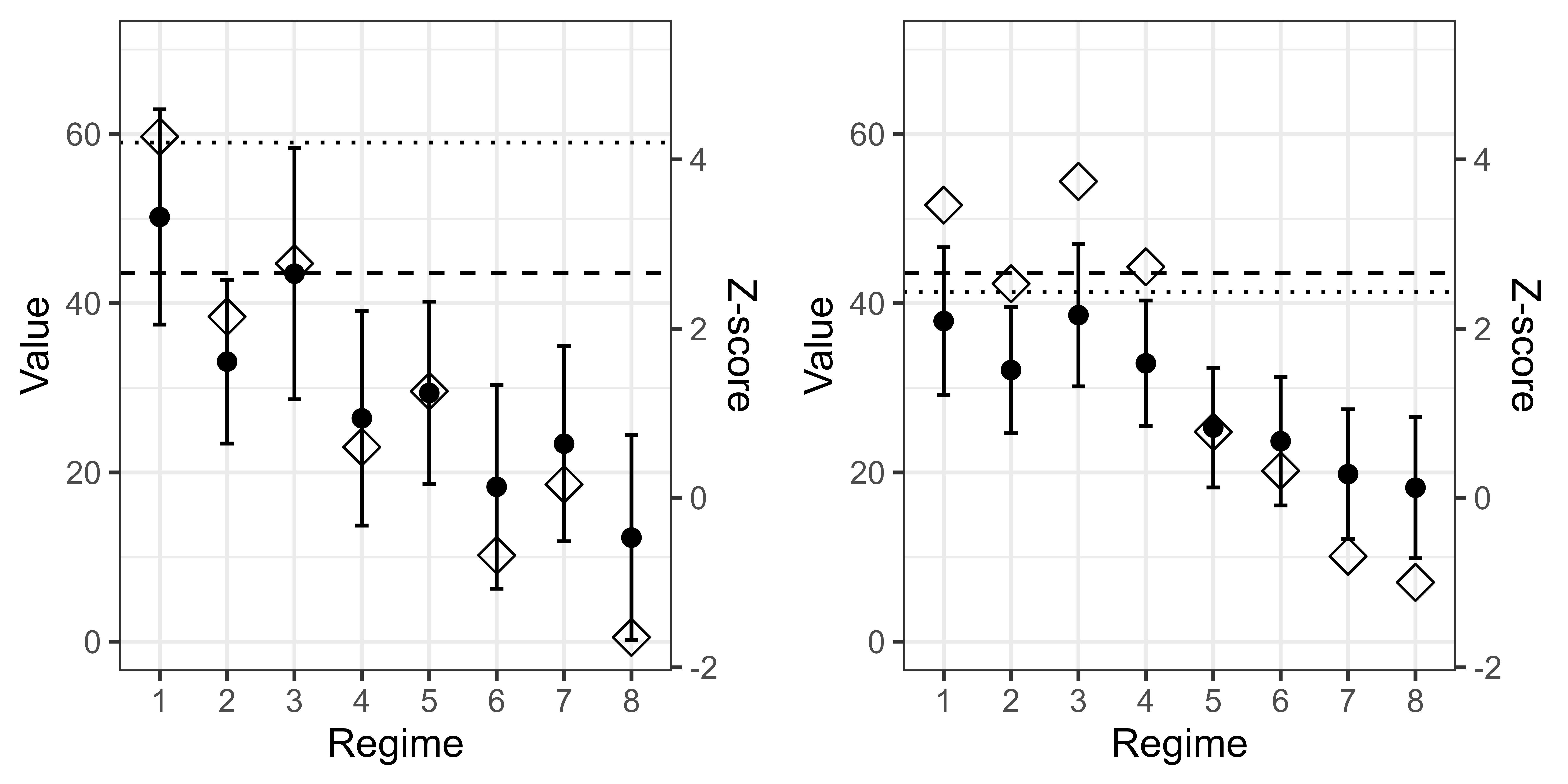
Figure 2: For the schema in Figure 1, interim analysis performance results for testing null hypothesis (2) against $H_{AD}$ with a fixed control. Results include the Pocock boundaries (dashed), OBF boundaries (dotted), value estimates (circles) and 95% confidence bounds, and test statistics (rhombus) at the interim (left) and final (right) analysis time for the behavioral pain management case study data set using the IAIPWE.

The interim analysis occurs at 500 days after the trial enrollment begins, at which point $51.4\%$ of the total planned sample size $N$ has been enrolled, $46.8\%$ of the $N$ planned participants have progressed to the second decision, and $34.9\%$ have completed the trial. Figure 2 summarizes the estimated values for each regime at the time of analysis, corresponding $Z$-statistic. Exact numbers are recorded in a tabular format in Appendix I. Regime 1, which starts with PCST-Full, triggers early stopping based on the test statistic exceeding the OBF boundary. Regimes 1 and 3 trigger early stopping based on test statistics exceeding the Pocock boundary. The standard errors are smaller than those obtained using the IPWE or AIPWE, which are included in the Appendix I. The IPWE and AIPWE trigger early stopping with regimes exceeding the Pocock boundary, but fail to trigger early stopping under the OBF boundary. The decision to stop the trial early reduces the sample size from the total possible $284$ subjects to $146$ and the length of the study by $96$ weeks. Early stopping means implementation of behavioral interventions for pain management in breast cancer patients, potentially helping more individuals and avoiding less efficacious regimes for those who otherwise would have enrolled in the trial.

8 Discussion

We proposed interim analysis methods for SMARTs that gain efficiency by using partial information from participants who have not yet completed all stages of the study. The approach yields a smaller expected sample size than competing methods while preserving type I error and power. Simulations demonstrate a potential for substantial resource savings.

We have demonstrated the methodology in the case of two-stage SMARTs with an interim analysis focused on evaluation of efficacy. However, the methods extend readily to studies with $K\geq 2$ decision points, multiple interim looks, and general hypotheses including futility. We have consider Pocock and OBF boundaries, though the approach can be adapted to any monitoring method, such as information-based monitoring (Tsiatis, 2006a, ) and the use of $\alpha$ spending functions (DeMets and Lan,, 1994).

We have made the simplifying assumptions throughout that: (i) the time between stages is fixed, which is the case for many SMARTs; and (ii) the final outcome is observed on all individuals by the end of the trial (so excluding the possibility of drop out). The extension to random times between stages is non-trivial. Simulations included in Appendix G suggest that the IAIPWE (incorrectly assuming fixed transition times) performs well when time per stage varies with subject outcomes. Due to variability in enrollment, an analysis at a predetermined time may have a realized power slightly different from the nominal power based on the number of individuals enrolled and their realized trajectories at the time of analysis. In such cases, planning the interim analysis based on available sample size rather than a pre-determined time may be preferred. Extensions for additional levels of coarsening, such as those due to drop out, attrition, or time-to-event outcomes requires additional augmentation terms or changes to the functions $\lambda_{r}^{\ell}(t),K_{r}^{\ell}(t)$ and $L_{k(r)}^{\ell}(\overline{\mathbf{x}}_{k(r)})$. For a comprehensive review of the considerations involved, see Chapter 8 of Tsiatis et al., (2020). A modified multiple imputation strategy may also be used for missing data following that of Shortreed et al., (2014).

As demonstrated in our simulation experiments, the sandwich covariance estimator can overestimate the variance of the values and lead to conservative stopping boundaries when the number of parameters is close to the sample size. Interim analyses typically have larger sample sizes, so this issue is unlikely to occur in practice. The information proportion can be checked at each interim analysis to verify the planned proportions against the realized values. The IAIPWE stopping boundary and sample size calculations also require the challenge of positing models. Although we have studied the performance of the IAIPWE under these conditions to evaluate fully its properties, we anticipate the trialists will prefer to power a SMART based on the IPWE to avoid making the additional model assumptions. We advocate this approach in practice as it can assuage concerns about misspecified models while still benefiting from the efficiency gains of the IAIPWE. If a trial does reach the final analysis, using the AIPWE offers efficiency gains by effectively performing covariate adjustment. Here, the covariates to be used in the $Q$-functions should be specified before the trial begins.

The framework presented here forms the basis for additional methodology for interim monitoring for SMARTs with random times between stages and specialized endpoints. The IAIPWE has potential use in adaptive trials in which randomization probabilities, or even the set of treatments, varies with accumulating information ((Jennison and Turnbull,, 2000, Chapter 17); Wang and Yee,, 2019). We will report on these developments in future work.

Supporting Information

R code for implementation is available from the authors.

Appendix A: Discussion on Coarsening

Some Examples of Coarsening

Consider the SMART from our data application and a subject who does not respond to PCST-Full and is subsequently given PCST-Plus, but has not yet reached their final follow up by interim analysis time $t_{1}$. When estimating the value of regime $1$, the patient is coarsened at level $\mathcal{R}^{1}(t_{1})=4$ because all treatments received are consistent with regime 1, but they have not completed the trial. However, when estimating the value of regime $3$, the subject is coarsened at level $\mathcal{R}^{3}(t_{1})=3$ because their first treatment is consistent with regime $3$, they made it to the second treatment assignment by the time of the interim analysis, but their second treatment is inconsistent with regime $3$. At the final analysis, after the subject completes their final follow up, the subject will have coarsening levels $\mathcal{R}^{1}(t_{S})=\infty$ and $\mathcal{R}^{3}(t_{S})=3$. The coarsening level when estimating the value of regime $1$ is now infinite because the subject finished the trial with treatments consistent with regime $1$; however, their coarsening level for regime $3$ remains the same because they were coarsened due to inconsistent treatments.

Coarsening Under Fixed Arrival Times

When arrival times for stages and treatment assignment are independent, we can simplify the notation for the IAIPW estimator to get the form for $K=2$ given in the paper. For ease of notation, let $A_{k}\in\{0,1\}$. Let $\pi_{k}^{d}(A_{k},\mathbf{H}_{k})=P(A_{k}=1|\mathbf{H}_{k})$, $\nu_{k}(t)=P(\kappa(t)\geq k|\Gamma(t)=1)$, and $C_{k}^{\ell}=\prod_{v=1}^{k}I\{A_{v}=d^{\ell}(\mathbf{H}_{v})\}$. We focus on the portion of the augmentation term without the arbitrary function, and suppress dependence on $t$ and $\ell$. Write

$$\frac{I\{\mathcal{R}=r\}-\lambda_{r}I\{\mathcal{R}\geq r\}}{K_{r}}=I\{\mathcal{R}\geq r\}\frac{I\{\mathcal{R}=r\}-\lambda_{r}}{K_{r}}.$$

Consider cases $r$ odd and even separately. Then

$$\begin{split}I\{\mathcal{R}\geq r\}\frac{I\{\mathcal{R}=r\}-\lambda_{r}}{K_{r}}&=I\{\mathcal{R}\geq r\}\left[\frac{I\{\mathcal{R}=r\}-P(\mathcal{R}=r|\mathcal{R}\geq r)}{P(\mathcal{R}>r)}\right]\\ &=I\{\mathcal{R}\geq r\}\left[\frac{I\{\mathcal{R}=r\}-\frac{P(\mathcal{R}=r)}{P(\mathcal{R}\geq r)}}{P(\mathcal{R}>r)}\right]\\ &=\begin{cases}I\{\mathcal{R}\geq r\}\left[\frac{I\{\mathcal{R}=r\}-P\left\{d_{k(r)}(\mathbf{H}_{k(r)})\neq A_{k(r)}\right\}}{P(\mathcal{R}>r)}\right]&\text{, r odd}\\ I\{\mathcal{R}\geq r\}\left[\frac{I\{\mathcal{R}=r\}-P\left\{\kappa=k(r)|\Gamma=1\right\}}{P(\mathcal{R}>r)}\right]&\text{, r even.}\\ \end{cases}\\ \end{split}$$

Simplify the probability statements using our propensities and enrollment notation, and the fact that the term is $0$ for all individuals coarsened before $r$. We can express the denominator as individuals who have been consistent with the regime through $k(r)-1$. Let $\pi_{0}=1$.

$$\begin{split}&=\begin{cases}I\{\mathcal{R}\geq r\}\left[\frac{I\{\mathcal{R}=r\}-\left\{C_{k(r)}(1-\pi_{k(r)}^{d})+(1-C_{k(r)})\pi_{k(r)}^{d}\right\}}{\nu_{k(r)}\left\{\prod_{k=0}^{k(r)-1}\pi_{k}^{d}\right\}\left\{C_{k(r)}\pi_{k(r)}^{d}+(1-C_{k(r)})(1-\pi_{k(r)}^{d})\right\}}\right]&\text{, r odd}\\ I\{\mathcal{R}\geq r\}\left[\frac{I\{\mathcal{R}=r\}-\left\{\nu_{k(r)}-\nu_{k(r)+1}\right\}}{\nu_{k(r)+1}\left\{\prod_{k=1}^{k(r)}\pi_{k}^{d}\right\}}\right]&\text{, r even}\\ \end{cases}\\ \end{split}$$

Further algebra and simplifications from $K=2$ yield the estimator in the paper. If the time to next treatment varies by treatment assignment, then the probability of coarsening due to time conditioned on the treatment assignment is no longer expressed with $\nu$ as defined and proper adjustments can be made.

Appendix B: Double Robustness Property of IAIPW Estimator

We show the estimator is consistent if either the propensity and proportion models are correctly specified, or the regression models are correctly specified. Let $\boldsymbol{\theta}_{p}$ characterize the parameters for the propensity and proportion models, and let $\boldsymbol{\theta}_{L}$ characterize those of the arbitrary function $L_{r}$. In both cases, we will assume for models chosen, $\widehat{\boldsymbol{\theta}}_{p}\overset{p}{\to}\boldsymbol{\theta}_{p}^{*}$ and $\widehat{\boldsymbol{\theta}}_{L}\overset{p}{\to}\boldsymbol{\theta}_{L}^{*}$, where $\boldsymbol{\theta}_{p}^{*}$ and $\boldsymbol{\theta}_{L}^{*}$ constant. If the models are correctly specified, then $\boldsymbol{\theta}_{p}^{*}=\boldsymbol{\theta}_{p}^{0}$ and $\boldsymbol{\theta}_{L}^{*}=\boldsymbol{\theta}_{L}^{0}$, respectively, superscript $0$ denoting true parameters. We assume that the enrollment process and treatment assignment and outcome are independent. For fixed $t$ and arbitrary $l$, the estimator converges to

$$\begin{split}&\mathbb{E}\bigg{[}\frac{I\left\{\mathcal{R}_{i}^{\ell}(t)=\infty\right\}}{\widehat{K}^{\ell}_{2K,i,n(t)}(t;\boldsymbol{\theta}^{*}_{p})}Y_{i}\\ &\quad+\sum_{r=1}^{2K}\frac{I\left\{\mathcal{R}^{\ell}_{i}(t)=r\right\}-\widehat{\lambda}^{\ell}_{r,i}(t;\boldsymbol{\theta}^{*}_{p})I\left\{\mathcal{R}^{\ell}_{i}(t)\geq r\right\}}{\widehat{K}^{\ell}_{r,i,n(t)}(t;\boldsymbol{\theta}^{*}_{p})}L^{\ell}_{k(r)}(\overline{\mathbf{X}}_{k(r),i};\boldsymbol{\theta}^{*}_{L,k(r)})\bigg{]}\\ &=\mathbb{E}\bigg{[}\frac{I\left\{\mathcal{R}_{i}^{\ell}(t)=\infty\right\}}{\widehat{K}^{\ell}_{2K,i,n(t)}(t;\boldsymbol{\theta}^{*}_{p})}Y^{*}(\mathbf{d}^{\ell})\bigg{]}+\\ &\quad\mathbb{E}\bigg{[}\sum_{r=1}^{2K}\frac{I\left\{\mathcal{R}^{\ell}_{i}(t)=r\right\}-\widehat{\lambda}^{\ell}_{r,i}(t;\boldsymbol{\theta}^{*}_{p})I\left\{\mathcal{R}^{\ell}_{i}(t)\geq r\right\}}{\widehat{K}^{\ell}_{r,i,n(t)}(t;\boldsymbol{\theta}^{*}_{p})}L^{\ell}_{k(r)}(\overline{\mathbf{X}}_{k(r),i};\boldsymbol{\theta}^{*}_{L,k(r)}).\bigg{]}\end{split}$$

By definition $Y_{i}I\{\mathcal{R}_{i}^{\ell}(t)=\infty\}=Y^{*}(\mathbf{d}^{\ell})$. By Lemma 10.4 of Tsiatis, 2006b ,

$$\begin{split}&\mathbb{E}\Bigg{(}Y^{*}(\mathbf{d}^{l})+\bigg{[}\frac{I\left\{\mathcal{R}_{i}^{\ell}(t)=\infty\right\}}{\widehat{K}^{\ell}_{2K,i,n(t)}(t;\boldsymbol{\theta}^{*}_{p})}-1\bigg{]}Y^{*}(\mathbf{d}^{\ell})\Bigg{)}+\\ &\quad\mathbb{E}\bigg{[}\sum_{r=1}^{2K}\frac{I\left\{\mathcal{R}^{\ell}_{i}(t)=r\right\}-\widehat{\lambda}^{\ell}_{r,i}(t;\boldsymbol{\theta}^{*}_{p})I\left\{\mathcal{R}^{\ell}_{i}(t)\geq r\right\}}{\widehat{K}^{\ell}_{r,i,n(t)}(t;\boldsymbol{\theta}^{*}_{p})}L^{\ell}_{k(r)}(\overline{\mathbf{X}}_{k(r),i};\boldsymbol{\theta}^{*}_{L,k(r)})\bigg{]}\\ &=\mathbb{E}\{Y^{*}(\mathbf{d})\}-\mathbb{E}\bigg{[}1-\frac{I\left\{\mathcal{R}_{i}^{\ell}(t)=\infty\right\}}{\widehat{K}^{\ell}_{2K,i,n(t)}(t;\boldsymbol{\theta}^{*}_{p})}\bigg{]}Y^{*}(\mathbf{d}^{\ell})+\\ &\quad\mathbb{E}\bigg{[}\sum_{r=1}^{2K}\frac{I\left\{\mathcal{R}^{\ell}_{i}(t)=r\right\}-\widehat{\lambda}^{\ell}_{r,i}(t;\boldsymbol{\theta}^{*}_{p})I\left\{\mathcal{R}^{\ell}_{i}(t)\geq r\right\}}{\widehat{K}^{\ell}_{r,i,n(t)}(t;\boldsymbol{\theta}^{*}_{p})}L^{\ell}_{k(r)}(\overline{\mathbf{X}}_{k(r),i};\boldsymbol{\theta}^{*}_{L,k(r)})\bigg{]}\\ &=\mathbb{E}\{Y^{*}(\mathbf{d})\}-\mathbb{E}\bigg{[}\sum_{r=1}^{2K}\frac{I\left\{\mathcal{R}^{\ell}_{i}(t)=r\right\}-\widehat{\lambda}^{\ell}_{r,i}(t;\boldsymbol{\theta}^{*}_{p})I\left\{\mathcal{R}^{\ell}_{i}(t)\geq r\right\}}{\widehat{K}^{\ell}_{r,i,n(t)}(t;\boldsymbol{\theta}^{*}_{p})}[Y^{*}(\mathbf{d})-L^{\ell}_{k(r)}(\overline{\mathbf{X}}_{k(r),i};\boldsymbol{\theta}^{*}_{L,k(r)})]\bigg{]}\end{split}$$

Therefore, the IAIPW estimator is consistent if the second term is 0. First, consider the case the propensity and proportion models are correctly specified. Then for $r=1,\dots,2K$, the hazard functions are correctly specified, i.e. $\lambda^{\ell}_{r,i}(t;\boldsymbol{\theta}^{*}_{p})=\lambda^{\ell*}_{r}(t)$ for all $r=1,\dots,2K$. Define $\mathcal{W}_{r,i}$ as the random vector $\{I(\mathcal{R}_{i}^{\ell}(t)=1),\dots,I(\mathcal{R}_{i}^{\ell}(t)=r-1),W_{i}\}$. Then by iterated expectations and the definition of the hazard functions, for all $r\neq\infty$,

$$\begin{split}&\mathbb{E}\bigg{[}\frac{\mathbb{E}[I\left\{\mathcal{R}^{\ell}_{i}(t)=r\right\}|\mathcal{W}_{r}]-\widehat{\lambda}^{\ell}_{r,i}(t;\boldsymbol{\theta}^{*}_{p})I\left\{\mathcal{R}^{\ell}_{i}(t)\geq r\right\}}{\widehat{K}^{\ell}_{r,i,n(t)}(t;\boldsymbol{\theta}^{*}_{p})}[Y^{*}(\mathbf{d})-L^{\ell}_{k(r)}(\overline{\mathbf{X}}_{k(r),i};\boldsymbol{\theta}^{*}_{L,k(r)})]\bigg{]}\\ &=\mathbb{E}\bigg{[}\frac{\widehat{\lambda}^{\ell}_{r,i}(t;\boldsymbol{\theta}^{*}_{p})I\left\{\mathcal{R}^{\ell}_{i}(t)\geq r\right\}-\widehat{\lambda}^{\ell}_{r,i}(t;\boldsymbol{\theta}^{*}_{p})I\left\{\mathcal{R}^{\ell}_{i}(t)\geq r\right\}}{\widehat{K}^{\ell}_{r,i,n(t)}(t;\boldsymbol{\theta}^{*}_{p})}[Y^{*}(\mathbf{d})-L^{\ell}_{k(r)}(\overline{\mathbf{X}}_{k(r),i};\boldsymbol{\theta}^{*}_{L,k(r)})]\bigg{]}\\ &=0.\end{split}$$

Now consider when the arbitrary functions $L^{\ell}_{k(r)}(\overline{\mathbf{X}}_{k(r),i};\boldsymbol{\theta}^{*}_{L,k(r)})$ are correctly specified for $\mathbb{E}\{Y^{*}(\mathbf{d})|\overline{\mathbf{X}}_{k}^{*}(\mathbf{d}_{k}^{\ell})=\mathbf{x}_{k}^{*}\}$. Under the assumption of coarsening at random and using iterated expectations on $[I\{\mathcal{R}^{\ell}_{i}(t)\geq r\},\overline{\mathbf{X}}_{k}^{*}(\mathbf{d}_{k}^{\ell})]$

$$\begin{split}&\mathbb{E}\bigg{[}\frac{I\left\{\mathcal{R}^{\ell}_{i}(t)=r\right\}-\widehat{\lambda}^{\ell}_{r,i}(t;\boldsymbol{\theta}^{*}_{p})I\left\{\mathcal{R}^{\ell}_{i}(t)\geq r\right\}}{\widehat{K}^{\ell}_{r,i,n(t)}(t;\boldsymbol{\theta}^{*}_{p})}[Y^{*}(\mathbf{d})-\mathbb{E}\{Y^{*}(\mathbf{d})|\overline{\mathbf{X}}_{k}^{*}(\mathbf{d}_{k}^{\ell})=\mathbf{x}_{k}^{*}\}]\bigg{]}\\ &\mathbb{E}\bigg{[}\frac{I\left\{\mathcal{R}^{\ell}_{i}(t)=r\right\}-\widehat{\lambda}^{\ell}_{r,i}(t;\boldsymbol{\theta}^{*}_{p})I\left\{\mathcal{R}^{\ell}_{i}(t)\geq r\right\}}{\widehat{K}^{\ell}_{r,i,n(t)}(t;\boldsymbol{\theta}^{*}_{p})}[\mathbb{E}\{Y^{*}(\mathbf{d})|\overline{\mathbf{X}}_{k}^{*}(\mathbf{d}_{k}^{\ell})=\mathbf{x}_{k}^{*}\}-\mathbb{E}\{Y^{*}(\mathbf{d})|\overline{\mathbf{X}}_{k}^{*}(\mathbf{d}_{k}^{\ell})=\mathbf{x}_{k}^{*}\}]\bigg{]}\\ &=0.\end{split}$$

Therefore the estimator is consistent if either the propensity or regression models are correctly specified.

Appendix C: Conditions and Proof of Theorem 1

Theorem 1 follows from the asymptotic results in Section 7 of Boos and Stefanski, (2013) with an adjustment to account for $n(t)$.

Let $\boldsymbol{\psi}(\mathbf{Y}(t),\mathbf{H}(t),\boldsymbol{\theta})$ be the set of equations such that

$$\boldsymbol{\psi}(\mathbf{Y}(t),\mathbf{H}(t),\boldsymbol{\theta})=\sum_{i=1}^{N}\boldsymbol{\psi}(Y_{i}\Delta_{i}(t),\mathbf{H}_{i}(t),\widehat{\boldsymbol{\theta}})=\mathbf{0}.$$

And, let $\boldsymbol{\theta}_{0}$ be the unique solution to $\mathbb{E}\{\boldsymbol{\psi}(\mathbf{Y}(t),\mathbf{H}(t),\boldsymbol{\theta}_{0})\}=\mathbf{0}$. Assume that

• $\boldsymbol{\psi}(\mathbf{Y}(t),\mathbf{H}(t),\boldsymbol{\theta})$ and its first two partial derivatives with respect to $\boldsymbol{\theta}(t)$ exist for all $\boldsymbol{\theta}$ in a neighborhood of $\boldsymbol{\theta}_{0}$, and is $o_{p}(N^{-1/2})$.

• The second derivative of $\boldsymbol{\psi}(\mathbf{Y}(t),\mathbf{H}(t),\boldsymbol{\theta})$ is bounded.

• $\mathbb{E}\{-\boldsymbol{\psi}^{\prime}(Y,\mathbf{H}(t),\boldsymbol{\theta}_{0})\}$ exists and is nonsingular.

• $\mathbb{E}\{\boldsymbol{\psi}(Y,\mathbf{H}(t),\boldsymbol{\theta}_{0})\boldsymbol{\psi}(Y,\mathbf{H}(t),\boldsymbol{\theta}_{0})^{T}\}$ exists and is finite.

• The proportion of individuals at the interim analysis time $t$ converges to a constant, i.e., $n(t)/N\overset{p}{\to}c>0$.

Then, $\sqrt{N}\{\widehat{\mathcal{V}}(t)-\mathcal{V}(t)\}\overset{d}{\to}\mathcal{N}(\mathbf{0},\boldsymbol{\Sigma}_{T})$ as $N\rightarrow\infty$ for

$$\boldsymbol{\Sigma}_{T}=\mathbf{1}\mathbb{E}\{-\boldsymbol{\psi}^{\prime}(Y,\mathbf{H}(t),\boldsymbol{\theta}_{0})\}^{-1}\mathbb{E}\{\boldsymbol{\psi}(Y,\mathbf{H}(t),\boldsymbol{\theta}_{0})\boldsymbol{\psi}(Y,\mathbf{H}(t),\boldsymbol{\theta}_{0})^{T}\}\mathbb{E}\{-\boldsymbol{\psi}^{\prime}(Y,\mathbf{H}(t),\boldsymbol{\theta}_{0})\}^{-1}\mathbf{1}$$

where $\mathbf{1}$ is the matrix $[\mathbf{0}|I_{L+1,L+1}]$ such that $\mathbf{1}\boldsymbol{\theta}=\mathcal{V}$.

While it may seem reasonable to consider the estimating equations purely as a function of observed individuals at an interim analysis, the estimation of the quantities $\Gamma_{i}(t)$ must be viewed as draws over $N$ individuals.

Proof:

For ease of notation, write

$$\widehat{V}_{IA}^{l}(t)=\frac{1}{n(t)}\sum_{i=1}^{N}\Gamma_{i}(t)V_{i}(t).$$

First, consider that $c$ may be estimated via estimating equation $0=\sum_{i=1}^{N}\Gamma_{i}-(1/c)$ if $n(t)$ is not fixed. Then, we can express the estimating equation for our estimator equivalently as

$$\begin{split}0&=\frac{1}{N}\sum_{i=1}^{N}\Gamma_{i}(t)\left\{\widehat{V}_{IA}^{l}(t)-V_{i}(t)\right\}c\\ &=c\frac{1}{N}\sum_{i=1}^{N}\Gamma_{i}(t)\left\{\widehat{V}_{IA}^{l}(t)-V_{i}(t)\right\}\\ &=\frac{1}{n(t)}\sum_{i=1}^{N}\Gamma_{i}(t)\left\{\widehat{V}_{IA}^{l}(t)-V_{i}(t)\right\}\\ &=\widehat{V}_{IA}^{l}(t)-\frac{1}{n(t)}\sum_{i=1}^{N}\Gamma_{i}(t)V_{i}(t)\\ \end{split}$$

Because the estimation remains a set of unbiased estimating equations, then by Theorem 7.2 of Boos and Stefanski, (2013) $\sqrt{N}\{\widehat{\mathcal{V}}(t)-\mathcal{V}(t)\}\overset{d}{\to}\mathcal{N}(\mathbf{0},\boldsymbol{\Sigma}_{T})$ as $N\rightarrow\infty$.

The result for contrast matrix $\mathbf{C}$ follows directly as $\sqrt{N}\{\mathbf{C}\widehat{\mathcal{V}}(t)-\mathbf{C}\mathcal{V}(t)\}\overset{d}{\to}\mathcal{N}(\mathbf{0},\mathbf{C}\boldsymbol{\Sigma}_{T}\mathbf{C}^{\top})$.

Appendix D: Stopping Boundaries and Power under Arbitrary $S$

We use the testing procedure outlined in the Section 5. To find stopping boundaries $\{c_{\alpha}(s)\}_{s=1}^{S}$ that control the family-wise error rate across all planned analyses at level $\alpha$, we use the joint distribution of the $Z$ statistics across all analyses. For chosen $\alpha$-spending function, the boundaries satisfy

$$P\{\text{Reject}\ H_{0D}|H_{0D}\ \text{is true}\}=P\left[\left.\bigcup_{\ell=1}^{L}\bigcup_{s=1}^{S}\{Z^{\ell}(t_{s})\geq c_{\alpha}(s)\}\right|H_{0D}\right]\leq\alpha,$$

which can be solved for by integration of the multivariate normal probability distribution function. For chosen stopping boundaries and specified alternative where the expectation of $\mathbf{Z}$ is $\boldsymbol{\mu}_{A}=\boldsymbol{\mu}_{A}\{n(t_{1}),\ldots,n(t_{S})\}$, the power is approximately

$$1-\int\dots\int_{D}\frac{1}{(2\pi)^{LS/2}\mathrm{det}(\boldsymbol{\Sigma}_{H})^{-1/2}}\mathrm{exp}\{-\frac{1}{2}(\mathbf{Z}-\boldsymbol{\mu}_{A})^{\top}\boldsymbol{\Sigma}_{H}^{-1}(\mathbf{Z}-\boldsymbol{\mu}_{A})\}dz^{1}(1)dz^{2}(1)\cdots dz^{L}(S)$$

for domain $D=(-\infty,c_{\alpha}(1)]\times(-\infty,c_{\alpha}(1)]\times\dots\times(-\infty,c_{\alpha}(S)]$, and one can solve for the sample sizes needed to achieve a specified power or the power for selected sample sizes.

Appendix E: Proof of Theorem 2

Proof

We can write the set of all estimating equations used in the IAIPW Estimator over time as $\mathrm{vec}\{\boldsymbol{\psi}(\mathbf{Y}(t_{s}),\mathbf{H}(t_{s}),\boldsymbol{\theta})\}_{s=1}^{S}$ where $\mathrm{vec}(\cdot)$ is the vectorization operator. Then under the conditions from Section B for times $\{t_{s}\}_{s=1}^{S}$,

$$\sqrt{N}[\mathrm{vec}\{\widehat{\mathcal{V}}(t_{s})\}_{s=1}^{S}-\mathrm{vec}\{\mathcal{V}(t)\}_{s=1}^{S}]\overset{d}{\to}\mathcal{N}(\mathbf{0},\boldsymbol{\Sigma}_{T_{s}})$$ (10)

for covariance $\boldsymbol{\Sigma}_{T_{s}}$ given in (7.10) in Boos and Stefanski, (2013) and the discussion below. Let $\mathbf{1}_{T}$ be the $SL\times S(L+1)$ matrix of block diagonal matrices $[-1_{1\times L}|I_{L\times L}]$. Then by Slutsky’s Theorem

$$\mathbf{Z}=\sqrt{N}\mathrm{diag}(\mathbf{1}_{T}\widehat{\boldsymbol{\Sigma}}_{T_{s}}\mathbf{1}_{T}^{\top})^{-1/2}\mathbf{1}_{T}[\mathrm{vec}\{\widehat{\mathcal{V}}(t_{s})\}_{s=1}^{S}-\mathrm{vec}\{\mathcal{V}(t)\}_{s=1}^{S}]\to\mathcal{N}(\boldsymbol{\mu}_{H},\boldsymbol{\Sigma}_{H})$$ (11)

where

$$\boldsymbol{\mu}_{H}=\mathbb{E}\left(\mathrm{diag}(\mathbf{1}_{T}\widehat{\boldsymbol{\Sigma}}_{T_{s}}\mathbf{1}_{T}^{\top})^{-1/2}\mathbf{1}_{T}[\mathrm{vec}\{\widehat{\mathcal{V}}(t_{s})\}_{s=1}^{S}-\mathrm{vec}\{\mathcal{V}(t)\}_{s=1}^{S}]\right)$$

and

$$\boldsymbol{\Sigma}_{H}=\mathrm{bdiag}(\mathbf{1}_{T}\boldsymbol{\Sigma}_{T_{s}}\mathbf{1}_{T}^{\top})^{-1/2}\mathbf{1}_{T}\boldsymbol{\Sigma}_{T_{s}}\mathbf{1}_{T}^{\top}\mathrm{bdiag}(\mathbf{1}_{T}\boldsymbol{\Sigma}_{T_{s}}\mathbf{1}_{T}^{\top})^{-1/2}.$$

Discussion

We can determine the value of $\iota$ given in Theorem 2 by finding the value of $\boldsymbol{\Sigma}_{H}$ for a general hypothesis, $H$, since $\iota^{-1}$ are entries $(1,L+1),(2,L+2),\ldots,(L,L+L)$ of $\boldsymbol{\Sigma}_{H}$. In the case that the information proportion varies between regimes, the $\iota^{-1,\ell}$ will be regime-specific.

The matrix $\boldsymbol{\Sigma}_{H}$ can be computed analytically. First, one must find the estimating equations used for all estimated parameter and stack these over all planned analyses. Then, the covariance of the estimating equations can be written as

$$\begin{split}\boldsymbol{\Sigma}_{\boldsymbol{\psi}}=&\mathbb{E}[-\mathrm{vec}\{\boldsymbol{\psi}^{\prime}(Y(t_{s}),\mathbf{H}(t_{s}),\boldsymbol{\theta}_{0})\}_{s=1}^{S}]^{-1}\times\\ &\mathbb{E}[\mathrm{vec}\{\boldsymbol{\psi}(Y(t_{s}),\mathbf{H}(t_{s}),\boldsymbol{\theta}_{0})\}_{s=1}^{S}\mathrm{vec}\{\boldsymbol{\psi}(Y(t_{s}),\mathbf{H}(t_{s}),\boldsymbol{\theta}_{0})\}_{s=1}^{S\quad\top}]\times\\ &\mathbb{E}[-\mathrm{vec}\{\boldsymbol{\psi}^{\prime}(Y(t_{s}),\mathbf{H}(t_{s}),\boldsymbol{\theta}_{0})\}_{s=1}^{S}]^{-1\top}\end{split}$$

following from Boos and Stefanski, (2013). However, this gives the covariance of all estimated parameters. We are interested in finding the covariance of the estimated values. Construct block diagonal matrix $\mathrm{bdiag}(\mathbf{1}_{1},\ldots,\mathbf{1}_{S})$ where $\mathbf{1}_{s}$ is the matrix $[0|I_{L+1,L+1}]$ such that $\mathbf{1}_{s}\boldsymbol{\theta}=\mathcal{V}$, as given in Appendix C. Then $\boldsymbol{\Sigma}_{T_{s}}=\mathrm{bdiag}(\mathbf{1}_{1},\ldots,\mathbf{1}_{S})\boldsymbol{\Sigma}_{\boldsymbol{\psi}}\mathrm{bdiag}(\mathbf{1}_{1},\ldots,\mathbf{1}_{S})^{\top}$. Let $\mathbf{1}_{T}$ be the matrix of $S$ block diagonal matrices $[-1_{1\times L}|I_{L\times L}]$. Then, following the application of Slutsky’s Theorem,

$$\begin{split}\boldsymbol{\Sigma}_{H}=&\mathrm{bdiag}\left(\mathbf{1}_{T}\mathrm{bdiag}(\mathbf{1}_{1},\ldots,\mathbf{1}_{S})\boldsymbol{\Sigma}_{\boldsymbol{\psi}}\mathrm{bdiag}(\mathbf{1}_{1},\ldots,\mathbf{1}_{S})^{\top}\mathbf{1}_{T}^{\top}\right)^{-1/2}\times\\ &\mathbf{1}_{T}\boldsymbol{\Sigma}_{\boldsymbol{\psi}}\mathbf{1}_{T}^{\top}\mathrm{bdiag}\left(\mathbf{1}_{T}\mathrm{bdiag}(\mathbf{1}_{1},\ldots,\mathbf{1}_{S})\boldsymbol{\Sigma}_{\boldsymbol{\psi}}\mathrm{bdiag}(\mathbf{1}_{1},\ldots,\mathbf{1}_{S})^{\top}\mathbf{1}_{T}^{\top}\right)^{-1/2\top}.\\ \end{split}$$

Appendix F: Sample Size Calculations for Wald-type Test Statistics

Below we outline how to determine the total planned sample size required to attain power $1-\beta$ for the Wald-type test statistic.

1. Choose $N$ sufficiently small such that the power at $N$ is below $1-\beta$.

2. Increase $N$ by $\lambda$ and update $\boldsymbol{\mu}_{A},\phi_{A}$.

3. Take $B$ draws from the distribution of $\mathbf{Z}$ and form the corresponding correlated sequential $\chi^{2}$ statistics.

4. Determine number of rejections under previously selected stopping boundaries $\{c_{\alpha}(s)\}$.

5. If simulated power exceeds tolerance of nominal power, and $\lambda\leq 1$, stop. Else, if simulated power exceeds tolerance of nominal power, and $\lambda>1$, update $\lambda$ by discount factor $\gamma<1$, go to step (2). Else, go to step (2)

The authors have initial values of $N=50$, $\lambda=10$, $\gamma=0.1$, and $B=10000$ to perform well in practice. We note that the information proportion for the interim AIPW estimator may require numerical simulation to estimate. However, the inverse of the information proportion is bounded between the proportion of individuals who have completed the study at interim analysis $s$ relative to the total planned planned sample size and the proportion of individuals who have enrolled in the study at interim analysis $s$ relative to the total planned planned sample size.

Appendix G: Additional Simulations

Regime Estimates for Additional Value Patterns

Table LABEL:tab:schema2_pocock_value_ests_vp13 summarizes the estimator used, the Monte Carlo mean value, standard deviation, and mean standard error for each estimator at both the interim analysis and final analysis. The mean square error (MSE) ratio is the ratio of the Monte Carlo MSE for the IPWE divided by that of the indicated method. A MSE ratio of greater than one indicates the estimator is more efficient than the IPWE. For (VP1), both the AIPWE and IAIPWE are more efficient than the IPWE at both analyses, and the IAIPWE is more efficient than the AIPWE. At the interim analysis, the standard errors for the IPWE underestimate the sampling variation in most cases, whereas the standard errors for the AIPWE overestimate the sampling variation. The IAIPWE consistently estimates the sampling variation with the exception of regime 6 at the interim analysis. The MC means demonstrate the consistency of the estimators as expected since the propensities are known in a SMART. Clearly, the IAIPWE estimates of the value for each regime more efficiently than the IPWE or AIPWE. Under (VP3) which has a smaller sample size than (VP1) to attain the power $80\%$, the IAIPWE and AIPWE are similarly efficient to the IPWE at the final analysis time. Therefore the IAIPWE is as efficient as the IPWE with a lower sample size. Here, the benefit of the IAIPWE is the lower overall sample size required for equivalent standard errors.

Table 4: For the schema in Figure 1, interim analysis performance results for testing hypothesis $H_{0D}$ against $H_{AD}$ with a fixed control value under Pocock Boundaries under (VP1) and (VP3) with method-based sample size $N$. MC Mean is the Monte Carlo mean of the estimates, MC SD is the Monte Carlo standard deviation of estimates, ASE is the Monte Carlo mean of the standard errors, and MSE Ratio is the ratio of the MC mean square error for the IPWE divided by that of the indicated estimator for the three estimates at the interim analysis (a) and final analysis (b) for $B=1000$ simulations.

VP		(a) Interim Analysis					(b) Final Analysis
	Method	Regime	MC Mean	MC SD	ASE	MSE Ratio		MC Mean	MC SD	ASE	MSE Ratio
1	IPWE	1	47.47	1.52	1.44	1.00		47.50	0.80	0.79	1.00
1	IPWE	2	47.52	1.51	1.44	1.00		47.52	0.84	0.79	1.00
1	IPWE	3	47.48	1.47	1.44	1.00		47.48	0.78	0.79	1.00
1	IPWE	4	47.53	1.48	1.44	1.00		47.51	0.82	0.79	1.00
1	IPWE	5	47.51	1.47	1.43	1.00		47.51	0.82	0.79	1.00
1	IPWE	6	47.55	1.43	1.44	1.00		47.55	0.78	0.79	1.00
1	IPWE	7	47.48	1.48	1.44	1.00		47.49	0.80	0.79	1.00
1	IPWE	8	47.52	1.47	1.44	1.00		47.53	0.76	0.79	1.00
1	AIPWE	1	47.47	1.43	1.47	1.14		47.48	0.76	0.77	1.11
1	AIPWE	2	47.50	1.42	1.46	1.13		47.51	0.76	0.76	1.22
1	AIPWE	3	47.49	1.39	1.46	1.13		47.47	0.75	0.76	1.06
1	AIPWE	4	47.52	1.40	1.47	1.12		47.50	0.75	0.76	1.21
1	AIPWE	5	47.50	1.39	1.46	1.12		47.49	0.77	0.76	1.12
1	AIPWE	6	47.53	1.33	1.45	1.16		47.53	0.75	0.76	1.08
1	AIPWE	7	47.42	1.45	1.45	1.04		47.46	0.78	0.76	1.05
1	AIPWE	8	47.44	1.41	1.46	1.07		47.51	0.72	0.77	1.13
1	IAIPWE	1	47.47	1.37	1.38	1.24		47.48	0.76	0.77	1.10
1	IAIPWE	2	47.50	1.37	1.36	1.21		47.51	0.76	0.76	1.21
1	IAIPWE	3	47.50	1.33	1.36	1.23		47.47	0.76	0.76	1.05
1	IAIPWE	4	47.53	1.35	1.38	1.20		47.50	0.75	0.77	1.21
1	IAIPWE	5	47.51	1.34	1.37	1.20		47.49	0.77	0.77	1.13
1	IAIPWE	6	47.54	1.27	1.35	1.26		47.53	0.75	0.76	1.08
1	IAIPWE	7	47.43	1.40	1.36	1.12		47.46	0.79	0.76	1.05
1	IAIPWE	8	47.46	1.36	1.37	1.16		47.51	0.72	0.77	1.12
3	IPWE	1	50.61	1.60	1.59	1.00		50.54	0.88	0.88	1.00
3	IPWE	2	49.04	1.61	1.60	1.00		49.02	0.93	0.88	1.00
3	IPWE	3	49.10	1.64	1.59	1.00		49.07	0.89	0.88	1.00
3	IPWE	4	47.53	1.59	1.59	1.00		47.54	0.87	0.88	1.00
3	IPWE	5	47.47	1.60	1.59	1.00		47.52	0.87	0.88	1.00
3	IPWE	6	47.52	1.59	1.58	1.00		47.51	0.87	0.87	1.00
3	IPWE	7	47.42	1.60	1.60	1.00		47.52	0.85	0.88	1.00
3	IPWE	8	47.47	1.54	1.59	1.00		47.52	0.86	0.88	1.00
3	AIPWE	1	50.61	1.64	1.72	0.95		50.55	0.86	0.88	1.06
3	AIPWE	2	49.10	1.60	1.69	1.00		49.04	0.88	0.88	1.12
3	AIPWE	3	49.06	1.61	1.7	1.03		49.07	0.86	0.88	1.08
3	AIPWE	4	47.56	1.54	1.7	1.07		47.56	0.87	0.88	1.00
3	AIPWE	5	47.49	1.58	1.71	1.02		47.50	0.88	0.88	0.97
3	AIPWE	6	47.51	1.55	1.69	1.04		47.52	0.85	0.88	1.03
3	AIPWE	7	47.44	1.58	1.71	1.03		47.52	0.89	0.88	0.91
3	AIPWE	8	47.46	1.58	1.72	0.95		47.53	0.86	0.88	1.00
3	IAIPWE	1	50.60	1.60	1.6	1.00		50.55	0.86	0.89	1.05
3	IAIPWE	2	49.10	1.57	1.57	1.04		49.04	0.88	0.89	1.12
3	IAIPWE	3	49.04	1.55	1.58	1.12		49.07	0.85	0.89	1.09
3	IAIPWE	4	47.55	1.50	1.58	1.12		47.56	0.87	0.89	1.00
3	IAIPWE	5	47.49	1.54	1.58	1.08		47.49	0.89	0.89	0.95
3	IAIPWE	6	47.51	1.51	1.55	1.11		47.51	0.86	0.88	1.02
3	IAIPWE	7	47.44	1.52	1.57	1.11		47.51	0.89	0.88	0.91
3	IAIPWE	8	47.46	1.53	1.59	1.01		47.53	0.86	0.88	1.00

Responders Receive a Single Treatment Option

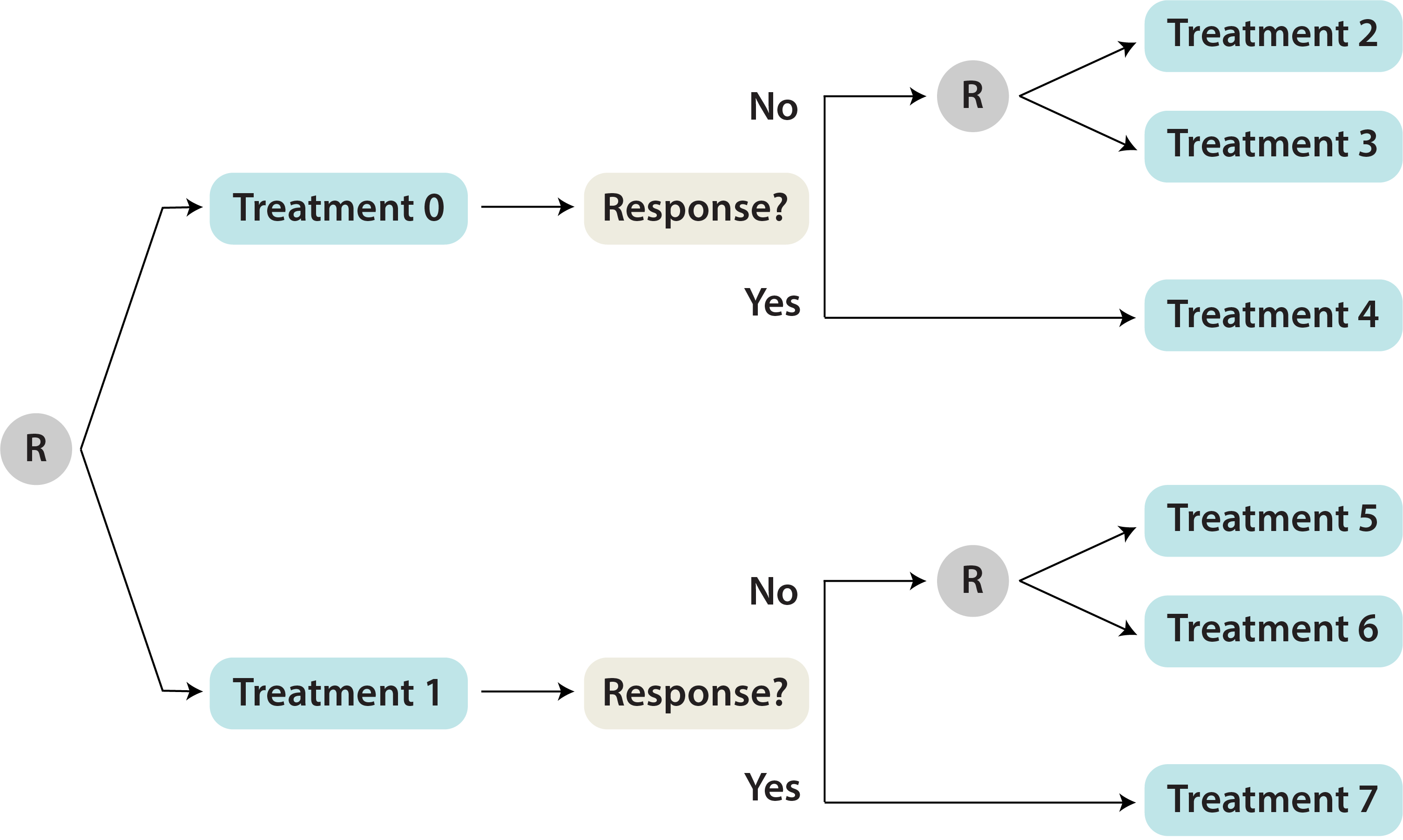
Figure 3: Schema in which responders only have one treatment available at stage $K=2$. The design embeds four regimes of the form ”Give intervention $a$; if non-response, give $b$; otherwise, if response give $c$.” Regimes $1,\ldots,4$ take $(a,b,c)$ to be $(0,2,4)$, $(0,3,4)$, $(1,5,7)$, and $(1,6,7)$, respectively.

We consider the trial design in Figure 3 and testing null hypothesis $H_{0D}$ for superiority. Enrollment times are drawn uniformly between 0 and 1000 days and follow-up times occur every 100 days. The first interim analysis is conducted when 30% of individuals have completed the trial which, under the enrollment mechanism, corresponds to having approximately 50% enrollment. We generate two baseline covariates $X_{1,1}\sim\mathrm{Uniform}(25,75)$ and $X_{1,2}\sim\mathrm{Bernoulli}(0.5)$ as well as an interim outcome $X_{2,1}\sim\mathrm{Uniform}(0,1)$ and response status $R_{2}\sim\mathrm{Bernoulli}(0.4)$; for notational consistency, $R_{2}$ is considered part of $\mathbf{X}_{2}$. The initial treatment is generated as $A_{1}\sim\mathrm{Bernoulli}(0.5)$ and, the second treatment is generated as $A_{2}|R_{2}=0\sim\mathrm{Bernouilli}(0.5)$ and $A_{2}|R_{2}=1$ is $0$. Outcomes are normally distributed with variance $\sigma^{2}=100$ and conditional mean

$$\mu_{S1}(\overline{\mathbf{X}}_{2},\overline{\mathbf{A}}_{2};\boldsymbol{\beta})=\beta_{0}+\beta_{1}X_{1,1}+\beta_{2}X_{1,2}+A_{1}\left\{\beta_{3}+\beta_{4}X_{1,1}+\beta_{5}X_{1,2}\right\}+\beta_{6}R_{2}X_{2,1}\\ +\beta_{7}(1-R_{2})X_{2,1}+(1-R_{2})A_{2}\left\{\beta_{8}+\beta_{9}A_{1}+\beta_{10}X_{1,1}+\beta_{11}X_{1,2}+\beta_{12}X_{2,1}\right\},$$

where $\boldsymbol{\beta}=(\beta_{0},\beta_{1},\ldots,\beta_{12})^{\top}$. Values of $\boldsymbol{\beta}$ were chosen to encode three value patterns (VPs): (VP1) all regimes are equivalent $(\boldsymbol{\beta}=(10,0.5,12.5,0,0,0,12.5,12.5,0,0,0,0,0)^{\top})$; (VP2) there is a single best embedded regime $(\boldsymbol{\beta}=(10,0.5,12.5,0,0,0,12.5,12.5,0,5,0,0,0)^{\top})$; and (VP3) embedded regimes starting with $A_{1}=0$ are optimal $(\boldsymbol{\beta}=(12.5,0.5,12.5,-2.5,0,0,\\ 12.5,12.5,0,0,0,0,0)^{\top})$. In (VP2), embedded regime $4$ attains a higher value $50.5$, and in (VP3), embedded regimes $1$ and $2$ attain the higher value $50.0$. All other regimes for each VP have value $47.5$. The clinically meaningful difference of $\delta=3$ and $2.5$ from the fixed control mean value $V(\mathbf{d}^{0})=47.5$ and nominal power $80\%$ are used for sample size calculations for (VP2) and (VP3), respectively.

Table 5 summarizes the true value pattern, the estimator used, the total planned sample size to achieve desired power under a specified alternative, the proportion of early rejections of $H_{0D}$, the proportion of total rejections, the expected sample size, and expected stopping time for analyses using the IPWE, AIPWE and IAIPWE. Results are presented for both when the sample size is determined for each estimator and when the sample for the IPWE is used for all estimators. The results may differ for each estimator as the IPWE and AIPWE use only individuals with complete trajectories. We calculate the total planned sample size to achieve power $80\%$ under (VP2) as the sample size for investigating the type I error rate under true (VP1), else to achieve power $80\%$ under the respective VPs. The expected sample size is average number of individuals enrolled in the trial regardless of their contribution to the estimator used when the trial is stopped. We test the null $H_{0D}$ against the alternative $H_{AD}$ for $\delta=0$ using the testing procedure outlined in the Section 5 with $S=2$ planned analyses at day $500$, and, if applicable, trial completion. We see that type I error rates are controlled and the nominal power is attained across three value pattern and stopping boundaries. The sandwich estimators of the variance of the values overestimates the asymptotic variance of the values for small $N$, which results in deflated early rejections for the AIPWE in these scenarios. The use of partial information for individuals by the IAIPWE results in smaller expected sample sizes and earlier expected stopping times for the alternative compared with the IPWE or AIPWE. As anticipated by the performance in conventional single-stage clinical trials, OBF boundaries may be too conservative if the analysis is performed when the proportion of information is low.

Table 5: For the schema in Figure 3, interim analysis performance results for testing $H_{0D}$ against $H_{AD}$ with a fixed control value using Pocock and OBF boundaries. Value pattern indicates the true value pattern. Method indicates the estimator used. The total planned sample size $N$ is determined by either each method (a) or by the IPWE (b). Total planned sample sizes are determined to maintain a nominal type I error rate of $\alpha=0.05$ and achieve a power of $80\%$ under the respective value patterns, using alternative (VP2) to determine the sample size for the null (VP1). Early Reject and Total Reject are the rejection rates at the first analysis and for the overall procedure, respectively. $\mathbb{E}$(SS) is the expected sample size, i.e, the average number of individuals enrolled in the trial when the trial is completed. $\mathbb{E}$(Stop) is the expected stopping time, i.e., the average number of days that the trial ran. Monte Carlo standard deviations are given in parentheses.

		(a) N Based on Method						(b) N Based on IPWE
VP	Method	N	Early Reject	Total Reject	$\mathbb{E}$(SS)	$\mathbb{E}$(Stop)		N	Early Reject	Total Reject	$\mathbb{E}$(SS)	$\mathbb{E}$(Stop)
1	IPWE	676		0.066	676 (0)	1199 (1)		676		0.066	676 (0)	1199 (1)
1	AIPWE	458		0.048	458 (0)	1198 (2)		676		0.058	676 (0)	1199 (1)
2	IPWE	676		0.798	676 (0)	1199 (1)		676		0.798	676 (0)	1199 (1)
2	AIPWE	458		0.783	458 (0)	1198 (2)		676		0.915	676 (0)	1199 (1)
3	IPWE	636		0.806	636 (0)	1199 (1)		636		0.806	636 (0)	1199 (1)
3	AIPWE	463		0.789	463 (0)	1198 (2)		636		0.907	636 (0)	1199 (1)
Pocock
1	IPWE	766	0.040	0.067	751 (75)	1171 (137)		766	0.040	0.067	751 (75)	1171 (137)
1	AIPWE	521	0.024	0.045	515 (39)	1181 (106)		766	0.027	0.050	756 (62)	1180 (113)
1	IAIPWE	517	0.047	0.065	505 (54)	1165 (148)		766	0.037	0.059	752 (72)	1173 (132)
2	IPWE	766	0.291	0.796	655 (174)	995 (318)		766	0.291	0.796	655 (174)	995 (318)
2	AIPWE	521	0.223	0.797	463 (108)	1042 (291)		766	0.357	0.923	630 (183)	949 (335)
2	IAIPWE	517	0.305	0.797	438 (119)	985 (322)		766	0.462	0.925	590 (191)	876 (349)
3	IPWE	730	0.308	0.809	617 (169)	984 (323)		730	0.308	0.809	617 (169)	984 (323)
3	AIPWE	532	0.265	0.810	461 (117)	1013 (308)		730	0.370	0.921	595 (177)	940 (338)
3	IAIPWE	524	0.355	0.804	431 (126)	950 (334)		730	0.486	0.926	553 (183)	859 (349)
O’Brien Fleming
1	IPWE	676	0.001	0.066	676 (11)	1198 (22)		676	0.001	0.066	676 (11)	1198 (22)
1	AIPWE	458	0.001	0.048	458 (7)	1197 (22)		676	0.001	0.058	676 (11)	1198 (22)
1	IAIPWE	459	0.002	0.048	459 (10)	1196 (31)		676	0.004	0.059	675 (21)	1196 (44)
2	IPWE	676	0.009	0.797	673 (32)	1192 (66)		676	0.009	0.797	673 (32)	1192 (66)
2	AIPWE	458	0.005	0.783	457 (15)	1194 (49)		676	0.015	0.915	671 (41)	1188 (85)
2	IAIPWE	459	0.033	0.784	451 (41)	1175 (124)		676	0.068	0.915	653 (85)	1151 (176)
3	IPWE	636	0.014	0.806	632 (37)	1189 (82)		636	0.014	0.806	632 (37)	1189 (82)
3	AIPWE	463	0.005	0.789	462 (49)	1194 (49)		636	0.010	0.906	633 (31)	1192 (70)
3	IAIPWE	463	0.051	0.789	451 (51)	1162 (154)		636	0.079	0.908	611 (86)	1143 (189)

Table 6 contains the same information as Table 5 when the $Q$-functions are misspecified by not including terms for $X_{1,1}$. The sample size to attain the desired power increases for the IAIPWE and AIPWE, but still remains smaller than the IPWE. The type I error rates are still controlled and the nominal power attained if the stopping boundaries are chosen under the misspecification.

Table 6: For the schema in Figure 3, interim analysis performance results for testing $H_{0D}$ against $H_{AD}$ with a fixed control value using Pocock and OBF boundaries. Summary of results as described in Table 5 when the $Q$-functions are misspecified.

VP	Method	$N$	Early Reject	Total Reject	$\mathbb{E}$(SS)	$\mathbb{E}$(Stop)
Single Analysis
1	IPWE	676		0.066	676 (0)	1199 (1)
1	AIPWE	579		0.060	579 (0)	1198 (2)
2	IPWE	676		0.798	676 (0)	1199 (1)
2	AIPWE	579		0.796	676 (0)	1198 (2)
3	IPWE	636		0.806	636 (0)	1198 (2)
3	AIPWE	562		0.811	562 (0)	1198 (2)
Pocock
1	IPWE	766	0.040	0.067	751 (75)	1178 (137)
1	AIPWE	659	0.034	0.059	648 (60)	1175 (127)
1	IAIPWE	654	0.048	0.068	638 (70)	1165 (149)
2	IPWE	766	0.291	0.796	655 (174)	995 (318)
2	AIPWE	659	0.231	0.791	583 (139)	1037 (295)
2	IAIPWE	654	0.294	0.803	558 (149)	993 (318)
3	IPWE	730	0.308	0.809	617 (169)	983 (333)
3	AIPWE	646	0.263	0.803	561 (142)	1015 (308)
3	IAIPWE	637	0.340	0.811	529 (151)	961 (331)
O’Brien Fleming
1	IPWE	676	0.001	0.066	676 (11)	1198 (22)
1	AIPWE	580	0.001	0.060	580 (9)	1198 (22)
1	IAIPWE	580	0.002	0.061	579 (12)	1196 (31)
2	IPWE	676	0.009	0.797	673 (32)	1192 (66)
2	AIPWE	580	0.009	0.798	577 (27)	1192 (66)
2	IAIPWE	580	0.036	0.798	570 (54)	1173 (130)
3	IPWE	636	0.014	0.806	632 (37)	1189 (82)
3	AIPWE	562	0.006	0.810	560 (21)	1194 (54)
3	IAIPWE	562	0.037	0.810	552 (53)	1172 (132)

Table 7 contains the same information as in Table 5 when testing the null hypothesis for homogeneity $H_{0H}$ using the $\chi^{2}$ testing procedure. We again calculate the sample size determined to achieve power $80\%$ under (VP2) as the sample size for investigating the type I error rate under true (VP1). We consider $S=2$ planned analyses at day $500$, and if applicable, trial completion. Table 7 shows that there is a slight increase in the total planned sample size required to achieve power equivalent to that for testing $H_{0D}$. The true OBF boundaries for a $\chi^{2}$ test make early stopping statistically improbable for interim analyses, which is reflected in the low early rejection rates and the difference between the expected sample size using OBF boundaries and the expected sample size performing a single analysis. The procedure achieves nominal power with a slightly inflated type I error rate.

Table 7: For the schema in Figure 3, interim analysis performance results for testing $H_{0H}$ against $H_{AH}$ with a fixed control value using Pocock and OBF boundaries under the $\chi^{2}$ testing procedure. Summary of results as described in Table 5.

VP	Method	$N$	Early Reject	Total Reject	$\mathbb{E}$(SS)	$\mathbb{E}$(Stop)
Single Analysis
1	IPWE	892		0.060	892 (0)	1199 (1)
1	AIPWE	473		0.049	473 (0)	1198 (2)
2	IPWE	892		0.772	892 (0)	1199 (1)
2	AIPWE	473		0.793	473 (0)	1198 (2)
3	IPWE	1377		0.783	1377 (0)	1198 (1)
3	AIPWE	773		0.766	773 (0)	1199 (1)
Pocock
1	IPWE	1045	0.035	0.055	1027 (95)	1175 (129)
1	AIPWE	559	0.044	0.065	547 (57)	1167 (143)
1	IAIPWE	537	0.066	0.092	519 (66)	1152 (173)
2	IPWE	1045	0.237	0.775	922 (222)	1033 (297)
2	AIPWE	559	0.271	0.792	484 (124)	1009 (311)
2	IAIPWE	537	0.324	0.803	450 (126)	972 (327)
3	IPWE	1581	0.239	0.777	1393 (336)	1032 (298)
3	AIPWE	903	0.225	0.774	802 (188)	1042 (291)
3	IAIPWE	867	0.320	0.777	729 (201)	975 (326)
O’Brien Fleming
1	IPWE	926	0.000	0.049	926 (0)	1199 (1)
1	AIPWE	497	0.000	0.043	497 (0)	1198 (2)
1	IAIPWE	484	0.001	0.047	484 (7)	1197 (22)
2	IPWE	926	0.003	0.803	925 (25)	1197 (22)
2	AIPWE	497	0.001	0.773	497 (8)	1197 (22)
2	IAIPWE	484	0.020	0.800	479 (34)	1184 (98)
3	IPWE	1395	0.003	0.773	1393 (37)	1197 (38)
3	AIPWE	796	0.002	0.760	795 (17)	1197 (31)
3	IAIPWE	778	0.019	0.765	771 (53)	1185 (95)

Finally, we consider $S=3$ with interim analyses at days $500$ and $700$. We test $H_{0D}$ against $H_{AD}$ with $\delta=0$. Table 8 contains the same entries as in Table 5 and the proportion of rejections that occur at the first analysis $s=1$, at the second analysis $s=2$ if the trial continued, and the total rejections if the $H_{0D}$ was rejected at any analysis. The IAIPWE again has the lowest expected sample size and earliest expected stopping times. For OBF boundaries, the total planned sample size is marginally higher for the IAIPWE than the AIPWE due to Monte Carlo error. Both nominal type I error rates and power are achieved.

Table 8: For the schema in Figure 3, interim analysis performance results for testing $H_{0D}$ against $H_{AD}$ with a fixed control value using Pocock and OBF boundaries. Summary of results as described in Table 5 with $S=3$ planned analyses on days $500,700,$ and trial end. Rejections for $s=1$ and $s=2$ are given as the proportion of rejections that occur at that analysis without a prior rejection.

VP	Method	$N$	Early Reject $s=1$	Early Reject $s=2$	Total Reject	$\mathbb{E}$(SS)	$\mathbb{E}$(Stop)
Single Analysis
1	IPWE	676			0.048	676 (0)	1198.6 (1)
1	AIPWE	458			0.046	458 (0)	1197.9 (2)
2	IPWE	676			0.784	676 (0)	1198.6 (1)
2	AIPWE	458			0.780	458 (0)	1197.9 (2)
3	IPWE	636			0.809	636 (0)	1198.5 (2)
3	AIPWE	462			0.807	462 (0)	1197.9 (2)
Pocock
1	IPWE	792	0.026	0.018	0.061	777 (70)	1172 (128)
1	AIPWE	540	0.023	0.013	0.050	532 (44)	1176 (118)
1	IAIPWE	532	0.039	0.017	0.070	519 (55)	1162 (148)
2	IPWE	792	0.264	0.200	0.788	641 (172)	915 (313)
2	AIPWE	540	0.218	0.200	0.789	449 (113)	946 (304)
2	IAIPWE	532	0.280	0.215	0.794	423 (116)	896 (314)
3	IPWE	759	0.313	0.205	0.820	594 (169)	878 (318)
3	AIPWE	552	0.274	0.213	0.804	441 (121)	901 (313)
3	IAIPWE	540	0.372	0.200	0.806	407 (122)	839 (319)
O’Brien Fleming
1	IPWE	679	0.000	0.006	0.051	678 (16)	1196 (16)
1	AIPWE	460	0.000	0.004	0.045	459 (9)	1196 (32)
1	IAIPWE	462	0.002	0.009	0.047	460 (16)	1192 (56)
2	IPWE	679	0.015	0.157	0.781	642 (83)	1110 (196)
2	AIPWE	460	0.007	0.122	0.780	442 (49)	1132 (171)
2	IAIPWE	462	0.039	0.207	0.773	424 (68)	1068 (231)
3	IPWE	639	0.017	0.174	0.808	600 (81)	1100 (204)
3	AIPWE	464	0.010	0.161	0.802	439 (55)	1111 (193)
3	IAIPWE	466	0.050	0.268	0.807	417 (75)	1030 (250)

Variable Time Between Analyses

For illustrative purposes, we consider the case when time between stages is not fixed. The outcomes are distributed as given in the previous setting where responders receive a single treatment. Enrollment times are drawn uniformly between $0$ and $1000$. Treatment two is assigned at a follow-up which occurs uniformly between $90$ and $110$ days after enrollment. The final outcome is observed uniformly between $90$ and $110$ days after treatment two is assigned.

Table 9: For the schema in Figure 3, interim analysis performance results for testing $H_{0D}$ against $H_{AD}$ with a fixed control value using Pocock and OBF boundaries. Summary of results as described in Table 5 when time between follow-ups is not fixed.

VP	Method	N	Early Reject	Total Reject	$\mathbb{E}$(SS)	$\mathbb{E}$(Stop)
1	IPWE	676		0.066	676 (0)	1206 (1)
1	AIPWE	458		0.048	458 (0)	1205 (2)
2	IPWE	676		0.798	676 (0)	1206 (1)
2	AIPWE	458		0.783	458 (0)	1205 (2)
3	IPWE	636		0.806	636 (0)	1206 (1)
3	AIPWE	463		0.789	463 (0)	1205 (2)
Pocock
1	IPWE	766	0.043	0.068	750 (78)	1177 (144)
1	AIPWE	521	0.025	0.046	515 (40)	1188 (110)
1	IAIPWE	517	0.047	0.066	505 (54)	1172 (149)
2	IPWE	766	0.282	0.794	658 (172)	1008 (318)
2	AIPWE	521	0.225	0.798	463 (109)	1046 (295)
2	IAIPWE	517	0.312	0.797	436 (120)	985 (327)
3	IPWE	730	0.305	0.811	618 (169)	991 (326)
3	AIPWE	532	0.268	0.810	461 (118)	1016 (313)
3	IAIPWE	524	0.362	0.805	429 (126)	950 (339)
O’Brien Fleming
1	IPWE	676	0.001	0.067	676 (10)	1206 (23)
1	AIPWE	458	0.001	0.048	458 (7)	1204 (23)
1	IAIPWE	459	0.002	0.048	459 (10)	1203 (32)
2	IPWE	676	0.010	0.797	673 (34)	1199 (70)
2	AIPWE	458	0.005	0.783	457 (15)	1201 (50)
2	IAIPWE	459	0.034	0.784	451 (42)	1181 (128)
3	IPWE	636	0.017	0.806	631 (41)	1194 (91)
3	AIPWE	463	0.003	0.789	462 (13)	1203 (39)
3	IAIPWE	463	0.046	0.789	452 (49)	1172 (148)

Table 9 contains the same entries as in Table 5 when the time between follow-ups is no longer fixed. We see that there is little difference in the performance of the estimators compared to when the time between stages is fixed. This suggests the IAIPWE is robust to variability in the time between follow-ups if this remains independent of the treatments.

Motivating Design with an Estimated Control Arm

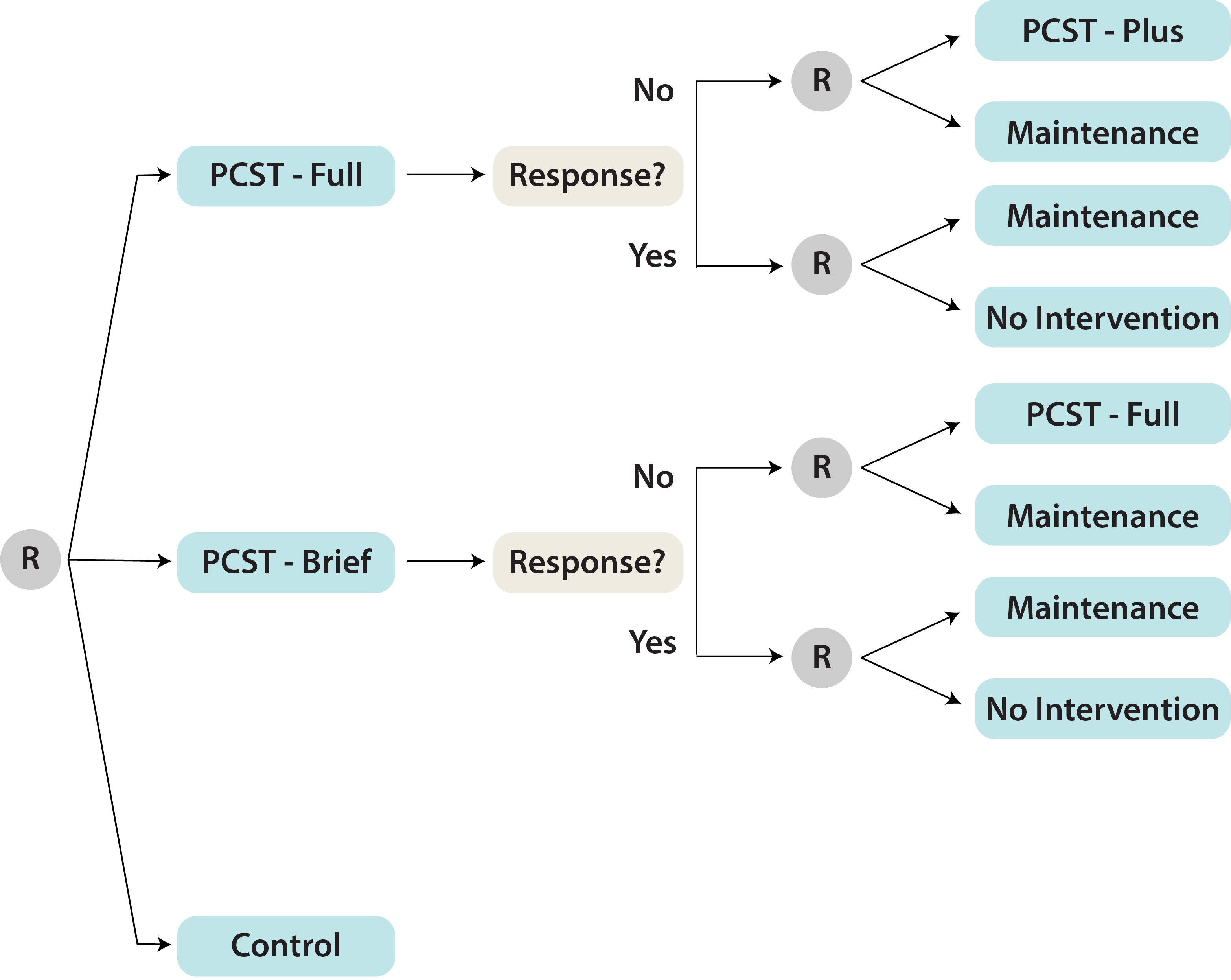
Figure 4: Schema for the SMART evaluating regimes involving behavioral interventions for pain management in breast cancer patients with an additional arm for standard of care.

We consider an additional schema with inclusion of a control arm shown in Figure 4. Individuals are randomly assigned to treatments labeled PCST-Full ($0$), PCST-Brief ($1$), or Control ($2$) with equal probability and enrolled in the trial as stated in trial design 1. We encode the control arm as treatment $A_{1}=2$ to align our notation with the mean model from the simulations in the Section 6. Interim analyses are conducted at day $700$ and trial end to mitigate over-estimation of the variance at day $500$ for small $n(t_{1})$. The outcome has variance $100$ and mean

$$\mu_{S3}(\overline{\mathbf{X}}_{2},\overline{\mathbf{A}}_{2})=\mu_{S2}(\overline{\mathbf{X}}_{2},\overline{\mathbf{A}}_{2})+I\left\{A_{1}=2\right\}\left(\beta_{26}+\beta_{27}X_{1,1}+\beta_{28}X_{1,2}+\beta_{29}X_{2,1}\right).\\$$

Let (VP2) indicate embedded regimes $\ell=1,\ldots,4$ attain a higher mean outcome than the standard of care by $\delta=3$. Let (VP3) indicate embedded regimes $\ell=1,\ldots,4$ attain a higher mean outcome than the standard of care by $\delta=5$.

Table 10 summarizes the results with entries as in Table 5. We use the sample size determined to achieve power $80\%$ under (VP2) as the sample size for investigating the type I error rate under (VP1), else the sample size is determined under the respective VP. We test the $H_{0D}$ against the alternative $H_{AD}$ for $\delta=0$ with $S=2$ planned analyses. As expected, estimation of a control arm increases the required sample size to achieve the same power when the control is fixed. Therefore, a more extreme treatment difference is required to have a similar overall sample size when estimating the mean under a control arm in a SMART. All methods attain the desired power, and the IAIPWE consistently has lower expected sample sizes than the IPWE and AIPWE. In some cases the AIPWE and IPWE have similar expected stopping times dues to the minimal difference in estimated information proportion or the over-estimated variance at the first analysis by the AIPWE. However, when the sample size of for all estimators is determined using the IPWE, the superiority of the AIPWE is seen in uniformly earlier stopping times and lower expected sample sizes. Differences in the total planned sample sizes for the IPWE under (a) and (b) are due to Monte Carlo error.

Table 10: For the schema in Figure 4, interim analysis performance results for testing $H_{0D}$ against $H_{AD}$ with a fixed control value using Pocock and OBF boundaries. Summary of results as described in Table 5.

		(a) N Based on Method						(b) N Based on IPWE
VP	Method	N	Early Reject	Total Reject	$\mathbb{E}$(SS)	$\mathbb{E}$(Stop)		N	Early Reject	Total Reject	$\mathbb{E}$(SS)	$\mathbb{E}$(Stop)
1	IPWE	1203		0.050	1203 (0)	1199 (1)		1203		0.050	1203 (0)	1199 (1)
1	AIPWE	1002		0.045	1002 (0)	1199 (1)		1203		0.048	1203 (0)	1199 (1)
2	IPWE	1203		0.791	1203 (0)	1199 (1)		1203		0.815	1203 (0)	1199 (1)
2	AIPWE	1002		0.794	1002 (0)	1199 (1)		1203		0.881	1203 (0)	1199 (1)
3	IPWE	433		0.817	433 (0)	1198 (2)		434		0.816	434 (0)	1198 (2)
3	AIPWE	361		0.790	361 (0)	1197 (3)		434		0.866	434 (0)	1198 (2)
Pocock
1	IPWE	1341	0.037	0.056	1326 (77)	1181 (94)		1342	0.033	0.058	1329 (72)	1183 (89)
1	AIPWE	1125	0.036	0.053	1113 (63)	1181 (93)		1342	0.027	0.045	1331 (65)	1186 (81)
1	IAIPWE	1122	0.038	0.055	1107 (78)	1180 (95)		1342	0.029	0.046	1328 (84)	1185 (84)
2	IPWE	1341	0.478	0.796	1149 (201)	961 (250)		1342	0.458	0.804	1158 (200)	971 (249)
2	AIPWE	1125	0.449	0.796	974 (168)	975 (248)		1342	0.543	0.871	1124 (201)	928 (249)
2	IAIPWE	1122	0.470	0.794	929 (205)	965 (249)		1342	0.565	0.872	1064 (244)	917 (248)
3	IPWE	484	0.528	0.827	407 (73)	935 (249)		483	0.499	0.821	411 (73)	949 (249)
3	AIPWE	406	0.438	0.811	353 (61)	980 (247)		483	0.511	0.877	409 (73)	943 (249)
3	IAIPWE	404	0.464	0.812	335 (74)	967 (248)		483	0.540	0.878	388 (88)	929 (248)
O’Brien Fleming
1	IPWE	1206	0.003	0.050	1205 (19)	1198 (27)		1207	0.002	0.054	1206 (17)	1198 (22)
1	AIPWE	1008	0.004	0.046	1007 (19)	1197 (32)		1207	0.000	0.052	1207 (0)	1199 (1)
1	IAIPWE	1007	0.007	0.047	1004 (31)	1195 (42)		1207	0.001	0.052	1207 (14)	1199 (16)
2	IPWE	1208	0.156	0.792	1150 (131)	1122 (181)		1207	0.167	0.820	1147 (135)	1116 (186)
2	AIPWE	1008	0.137	0.798	967 (104)	1131 (172)		1207	0.201	0.877	1134 (145)	1099 (200)
2	IAIPWE	1007	0.175	0.797	943 (140)	1112 (190)		1207	0.250	0.876	1097 (192)	1074 (216)
3	IPWE	434	0.189	0.821	409 (51)	1104 (195)		435	0.185	0.814	411 (50)	1106 (193)
3	AIPWE	363	0.124	0.792	349 (36)	1136 (164)		435	0.164	0.866	414 (48)	1116 (184)
3	IAIPWE	363	0.166	0.792	341 (50)	111 (185)		435	0.222	0.866	400 (66)	1087 (207)

Appendix H: Generative Models for Data Application

Using the generative model below, the expected outcome for regimes $\ell=1,\ldots,8$ are $(37.5,35.0,35.0,32.5,26.5,23.0,23.0,19.5)$.

Table 11: Generative model for cancer pain SMART. $\boldsymbol{\beta}=(\beta_{0},\beta_{1},\ldots,\beta_{12})^{\top}=(1,0,0.2,0,10,-10,1,0,-10,-5,-2,10,-2)^{\top}$.

Variable	Description	Distribution
$X_{1,1}$	height (cm)	$\mathrm{Normal}(152,25)$
$X_{1,2}$	weight (kg)	$\mathrm{Normal}(55,100)$
$X_{1,3}$	comorbidities	$\mathrm{Bernoulli}(0.6)$
$X_{1,4}$	use of pain medication	$\mathrm{Bernoulli}(0.4)$
$X_{1,5}$	received chemo	$\mathrm{Bernoulli}(0.6)$
$A_{1}$	initial treatment	$\mathrm{Bernoulli}(0.5)$
$R_{2}$	response	$\mathrm{Bernoulli}(0.5)$
$X_{2,0}$	reduction in pain	$\mathrm{Uniform}(30,40)$ if $R_{2}=1$ and $\mathrm{Uniform}(0,20)$ otherwise
$X_{2,1}$	adherence	$\mathrm{Uniform}(0.5,1)$
$A_{2}$	second treatment	$\mathrm{Bernoulli}(0.5)$
$Y$	response	$\beta_{0}+\beta_{1}X_{1,1}+\beta_{2}X_{1,2}+\beta_{3}X_{1,3}+\beta_{4}X_{,14}+\beta_{5}X_{1,5}+\beta_{6}X_{2,0}+\beta_{7}X_{2,1}+\beta_{8}A_{1}+\beta_{9}A_{2}+\beta_{10}A_{1}A_{2}+\beta_{11}R_{2}+\beta_{12}A_{1}R_{2}+\epsilon$
$\epsilon$	error	$\mathrm{Normal}(0,900)$

The fixed control value of 22.5% is based on positing that the average responder and non-responder exhibit a 30% and 15% reduction in pain, respectively. Consistent with the null hypothesis of no treatment difference, the response status at week eight under null hypothesis (2) would be similar between regimes. Because the final outcome is measured at six months, participants who respond to the first stage treatment may still exhibit different treatment effects across regimes.

Appendix I: Data Application Tabular Results

Table 12: Pocock boundaries, OBF boundaries, estimated values $\times 10^{-1}$ (standard errors), and test statistics at interim and final analysis time for the behavioral pain management case study data set using the IPWE. Results are presented for the interim analysis (a) then the final analysis (b).

	(a) Interim Analysis				(b) Final Analysis
Regime	Pocock	OBF	Value (SE)	$Z$-score	Pocock	OBF	Value (SE)	$Z$-score
1	2.66	4.30	5.13 (7.06)	2.12	2.66	2.44	3.75 (4.57)	3.28
2	2.66	4.30	3.23 (5.54)	1.82	2.66	2.44	3.26 (3.93)	2.56
3	2.66	4.30	4.71 (9.06)	1.78	2.66	2.44	3.87 (4.48)	3.61
4	2.66	4.30	2.81 (7.72)	1.46	2.66	2.44	3.38 (3.84)	2.93
5	2.66	4.30	2.85 (6.12)	0.46	2.66	2.44	2.53 (3.64)	0.78
6	2.66	4.30	1.57 (6.15)	0.27	2.66	2.44	2.42 (4.08)	0.41
7	2.66	4.30	2.19 (6.16)	$-$0.61	2.66	2.44	1.87 (3.96)	$-$0.95
8	2.66	4.30	0.90 (5.91)	$-$0.83	2.66	2.44	1.76 (4.35)	$-$1.13

Table 13: Pocock boundaries, OBF boundaries, estimated values $\times 10^{-1}$ (standard errors), and test statistics at interim and final analysis time for the behavioral pain management case study data set using the AIPWE. Results are presented for the interim analysis (a) then the final analysis (b).

	(a) Interim Analysis				(b) Final Analysis
Regime	Pocock	OBF	Value (SE)	$Z$-score	Pocock	OBF	Value (SE)	$Z$-score
1	2.66	4.30	4.97 (6.87)	3.96	2.66	2.44	3.79 (4.45)	3.46
2	2.66	4.30	3.29 (5.20)	1.99	2.66	2.44	3.21 (3.81)	2.53
3	2.66	4.30	4.33 (8.05)	2.58	2.66	2.44	3.86 (4.3)	3.74
4	2.66	4.30	2.65 (6.53)	0.61	2.66	2.44	3.29 (3.79)	2.73
5	2.66	4.30	2.87 (5.70)	1.09	2.66	2.44	2.53 (3.61)	0.78
6	2.66	4.30	1.81 (6.19)	$-$0.70	2.66	2.44	2.37 (3.88)	0.32
7	2.66	4.30	2.21 (6.09)	$-$0.06	2.66	2.44	1.98 (3.91)	$-$0.69
8	2.66	4.30	1.15 (6.28)	$-$1.75	2.66	2.44	1.82 (4.26)	$-$1.00

Table 14: Interim analysis performance results for testing null hypothesis $H_{0D}$ against $H_{AD}$ with a fixed control. Results include the Pocock boundaries, OBF boundaries, value estimates $\times 10^{-1}$ (standard errors), and test statistics at interim and final analysis time for the behavioral pain management case study data set using the IAIPWE. Results are presented for the interim analysis (a) then the final analysis (b).

	(a) Interim Analysis				(b) Final Analysis
Regime	Pocock	OBF	Value (SE)	$Z$-score	Pocock	OBF	Value (SE)	$Z$-score
1	2.66	4.20	5.02 (6.49)	4.27	2.66	2.43	3.79 (4.45)	3.46
2	2.66	4.20	3.31 (4.94)	2.14	2.66	2.43	3.21 (3.81)	2.53
3	2.66	4.20	4.35 (7.58)	2.77	2.66	2.43	3.86 (4.3)	3.74
4	2.66	4.20	2.64 (6.47)	0.60	2.66	2.43	3.29 (3.79)	2.73
5	2.66	4.20	2.94 (5.51)	1.26	2.66	2.43	2.53 (3.61)	0.78
6	2.66	4.20	1.83 (6.14)	$-$0.68	2.66	2.43	2.37 (3.88)	0.32
7	2.66	4.20	2.34 (5.89)	0.16	2.66	2.43	1.98 (3.91)	$-$0.69
8	2.66	4.20	1.23 (6.19)	$-$1.65	2.66	2.43	1.82 (4.26)	$-$1.00

Appendix J: Independent Increments for Independent Enrollment and Propensities

Without the augmentation terms, the independent increments property follows intuitively because there is no correlation between outcomes for different individuals. When considering the augmentation terms, it is not immediately obvious that independent increments holds. The property of independent increments follows from the form of the estimator and can hold when the correlation between sequential observations is non-zero. The influence function of our estimator has a martingale structure, which leads to many of the cross-term covariances among sequential influence functions to be zero. The non-zero covariances exhibit an interesting pattern where portions of the cross-term covariances for different terms cancel out. What is left after summing these terms is the variance of the influence function at a single analysis time, proving the independent increments. We may consider this as a result of the coarsening structure of the estimator appropriately accounting for how information will be accumulated over time. Therefore, even though individuals may have correlated information between analysis times, the estimator possesses the independent increments property.

Estimated values of regimes at the same analysis time may be correlated. From the previous results at any interim analysis $s$, $\sqrt{N}\{\widehat{\mathcal{V}}(t_{s})-\mathcal{V}(t_{s})\}\overset{d}{\to}\mathcal{N}(\mathbf{0},\boldsymbol{\Sigma}_{T})$ and $\sqrt{N}\{\mathbf{1}\widehat{\mathcal{V}}(t_{s})-\mathbf{1}\mathcal{V}(t_{s})\}\overset{d}{\to}\mathcal{N}(\mathbf{0},\mathbf{1}\boldsymbol{\Sigma}_{T}\mathbf{1}^{\top})$.

Denote the information at analysis $s$ as $\mathcal{I}(t_{s})=n(t_{s})(\mathbf{1}\boldsymbol{\Sigma}_{T}\mathbf{1}^{\top})^{g}$. Then, let $W(t_{s})=\mathcal{I}(t_{s})\mathbf{1}\widehat{\mathcal{V}}(t_{s})$. It is straightforward to see

$$\begin{split}&\mathbb{E}W(t_{s})=\mathcal{I}(t_{s})\mathbf{1}{\mathcal{V}}(t_{s})\\ &\mathrm{var}W(t_{s})=\mathcal{I}(t_{s})\mathbf{1}\boldsymbol{\Sigma}_{T}\mathbf{1}^{\top}/n(t_{s})\mathcal{I}(t_{s})=\mathcal{I}(t_{s}).\\ \end{split}$$

Define the influence functions for the IAIPW estimator with $C_{r}$ for ease of notation as

$$IF^{l}(t_{s})=YC_{0}(t_{s})+\sum_{r=1}^{2K}\left[C_{r}(t_{s})\mathbb{E}\{Y^{*}(\mathbf{d})|\overline{X}_{k(r)-1},{X}^{*}_{k(r)}\}\right]-\mathbb{E}\{Y^{*}(\mathbf{d})\}$$

It is sufficient to show independent increments by showing that the influence functions of the estimator $V_{IA}^{l}(t_{s})$, $\mathrm{cov}\{IF^{l}(t_{s}),IF^{l}(t_{s^{\prime}})\}=\mathrm{var}\{IF^{l}(t_{s^{\prime}})\}$ for $t_{s}<t_{s^{\prime}}$.

By construction, $\mathbb{E}\{IF^{l}(t_{s})\}=0$. Furthermore, $\sum_{r=0}^{2K}C_{r}=1$ for individuals enrolled in the study. Thus,

$$IF^{l}(t_{s})=Y^{*}(\mathbf{d})-\mathbb{E}\{Y^{*}(\mathbf{d})\}-\sum_{r=1}^{2K}C_{r}(t_{s})\left[Y^{*}(\mathbf{d})-\mathbb{E}\{Y^{*}(\mathbf{d})|\overline{X}_{k(r)-1},{X}^{*}_{k(r)}\}\right]$$ (12)

We will begin by showing that these terms have a martingale structure. In particular, we will show that the expectation of the cross terms for $r\neq r^{\prime}\pm 1$ is $0$. Let

$$\xi_{k(r)}(t_{s})=\{X_{1},A_{1},\kappa_{1},\dots,X_{k(r)-1},A_{k(r)-1},\kappa_{k(r)-1},I(\kappa_{k(r)}=k(r))X_{k(r)},X_{k(r)}^{*}(\mathbf{d}),Y^{*}(d)\},$$

and suppress $t_{s}$ when we consider only one analysis.

$$\begin{split}&\mathbb{E}\Big{(}C_{r}(t_{s})\big{[}Y^{*}(\mathbf{d})-\mathbb{E}\{Y^{*}(\mathbf{d})|\overline{X}_{k(r)-1},{X}^{*}_{k(r)}\}\big{]}C_{r^{\prime}}(t_{s})\big{[}Y^{*}(\mathbf{d})-\mathbb{E}\{Y^{*}(\mathbf{d})|\overline{X}_{k(r^{\prime})-1},{X}^{*}_{k(r^{\prime})}\}\big{]}\Big{)}\\ &=\mathbb{E}\bigg{\{}C_{r}(t_{s})\big{[}Y^{*}(\mathbf{d})-\mathbb{E}\{Y^{*}(\mathbf{d})|\overline{X}_{k(r)-1},{X}^{*}_{k(r)}\}\big{]}\times\\ &\hskip 14.22636pt\mathbb{E}\Big{(}C_{r^{\prime}}(t_{s})\big{[}Y^{*}(\mathbf{d})-\mathbb{E}\{Y^{*}(\mathbf{d})|\overline{X}_{k(r^{\prime})-1},{X}^{*}_{k(r^{\prime})}\}\big{]}|\xi_{k(r^{\prime})-1}\Big{)}\bigg{\}}\\ &=\mathbb{E}\bigg{\{}C_{r}(t_{s})\big{[}Y^{*}(\mathbf{d})-\mathbb{E}\{Y^{*}(\mathbf{d})|\overline{X}_{k(r)-1},{X}^{*}_{k(r)}\}\big{]}\times 0\bigg{\}}\\ &=0.\\ \end{split}$$

Similarly,

$$\mathbb{E}\Big{(}[Y^{*}(\mathbf{d})-\mathbb{E}\{Y^{*}(\mathbf{d})\}]C_{r^{\prime}}(t_{s})\big{[}Y^{*}(\mathbf{d})-\mathbb{E}\{Y^{*}(\mathbf{d})|\overline{X}_{k(r^{\prime})-1},{X}^{*}_{k(r^{\prime})}\}\big{]}\Big{)}=0.\\$$

Therefore

$$\mathrm{var}\{IF^{l}(t_{s})\}=\mathrm{var}\{Y^{*}(\mathbf{d})\}+\sum_{k=1}^{K}\mathbb{E}\bigg{(}\{C_{2k-1}(t_{s})+C_{2k}(t_{s})\}\left[Y^{*}(\mathbf{d})-\mathbb{E}\{Y^{*}(\mathbf{d})|\overline{X}_{k-1},{X}^{*}_{k}\}\right]\bigg{)}^{2}$$ (13)

Now, we consider the covariance between influence functions at two time points, $t_{s}$ and $t_{s^{\prime}}$ for $s<s^{\prime}$. By the martingale structure,

$$\begin{split}&\mathrm{cov}\Big{(}[Y^{*}(\mathbf{d})-\mathbb{E}\{Y^{*}(\mathbf{d})\}],C_{r}(t_{s})\left[Y^{*}(\mathbf{d})-\mathbb{E}\{Y^{*}(\mathbf{d})|\overline{X}_{k(r)-1},{X}^{*}_{k(r)}\}\right]\Big{)}=0,\\ &\mathrm{cov}\Big{(}[Y^{*}(\mathbf{d})-\mathbb{E}\{Y^{*}(\mathbf{d})\}],C_{r}(t_{s^{\prime}})\left[Y^{*}(\mathbf{d})-\mathbb{E}\{Y^{*}(\mathbf{d})|\overline{X}_{k(r)-1},{X}^{*}_{k(r)}\}\right]\Big{)}=0,\mathrm{and}\\ &\mathrm{cov}\Big{(}C_{r^{\prime}}(t_{s})\left[Y^{*}(\mathbf{d})-\mathbb{E}\{Y^{*}(\mathbf{d})|\overline{X}_{k(r^{\prime})-1},{X}^{*}_{k(r^{\prime})}\}\right],C_{r}(t_{s^{\prime}})\left[Y^{*}(\mathbf{d})-\mathbb{E}\{Y^{*}(\mathbf{d})|\overline{X}_{k(r)-1},{X}^{*}_{k(r)}\}\right]\Big{)}=0\end{split}$$

for $r<r^{\prime}+1$ and $s<s^{\prime}$. We will show that

$$\begin{split}&\mathbb{E}\Big{(}\sum_{k=1}^{k^{\prime}}\{C_{2k-1}(t_{s})+C_{2k}(t_{s})\}\left[Y^{*}(\mathbf{d})-\mathbb{E}\{Y^{*}(\mathbf{d})|\overline{X}_{k-1},{X}^{*}_{k}\}\right]\times\\ &\hskip 28.45274pt\{C_{2k^{\prime}-1}(t_{s^{\prime}})+C_{2k^{\prime}}(t_{s^{\prime}})\}\left[Y^{*}(\mathbf{d})-\mathbb{E}\{Y^{*}(\mathbf{d})|\overline{X}_{k^{\prime}-1},{X}^{*}_{k^{\prime}}\}\right]\Big{)}\\ &=\mathbb{E}\Big{(}\{C_{2k^{\prime}-1}(t_{s^{\prime}})+C_{2k^{\prime}}(t_{s^{\prime}})\}\left[Y^{*}(\mathbf{d})-\mathbb{E}\{Y^{*}(\mathbf{d})|\overline{X}_{k^{\prime}-1},{X}^{*}_{k^{\prime}}\}\right]\Big{)}^{2}.\\ \end{split}$$

for the case $K=2$ to show that independent increments holds.

$$\begin{split}&\mathbb{E}\Big{(}\sum_{k=1}^{k^{\prime}}\{C_{2k-1}(t_{s})+C_{2k}(t_{s})\}\left[Y^{*}(\mathbf{d})-\mu_{k}\right]\{C_{2k^{\prime}-1}(t_{s^{\prime}})+C_{2k^{\prime}}(t_{s^{\prime}})\}\left[Y^{*}(\mathbf{d})-\mu_{k^{\prime}}\right]\Big{)}\\ &=\mathbb{E}\Big{(}\{C_{2k^{\prime}-1}(t_{s})+C_{2k^{\prime}}(t_{s})\}\left[Y^{*}(\mathbf{d})-\mu_{k^{\prime}}\right]\Big{)}^{2}.\\ \end{split}$$

Let $r$ be odd and let $\nu_{k}(t_{s})=pr\{\kappa(t_{s})\geq k|\Gamma(t_{s})=1\}$ and $\nu_{K+1}(t_{s})=pr\{\Delta(t_{s})=1|\Gamma(t_{s})=1\}$. We make use of the abused notation that $k(r)=k(r+1)=k$ and begin by simplifying part of the expressions we will need.

$$C_{r}(t_{s})+C_{r+1}(t_{s})=\frac{I\{\mathcal{R}(t_{s})=r\}-pr\{\mathcal{R}(t_{s})=r|\mathcal{R}(t_{s})\geq r,W(t_{s})\}I\{\mathcal{R}(t_{s})\geq r\}}{pr\{\mathcal{R}(t_{s})>r|W(t_{s})\}}+\\ \frac{I\{\mathcal{R}(t_{s})=r+1\}-pr\{\mathcal{R}(t_{s})=r+1|\mathcal{R}(t_{s})\geq r+1,W(t_{s})\}I\{\mathcal{R}(t_{s})\geq r+1\}}{pr\{\mathcal{R}(t_{s})>r+1|W(t_{s})\}}\\ =\frac{I\{\mathcal{R}(t_{s})=r\}-\{1-\pi_{k}(\mathbf{d})\}I\{\mathcal{R}(t_{s})\geq r\}}{\nu_{k}(t_{s})\prod_{\tilde{k}=1}^{k}\pi_{\tilde{k}}(\mathbf{d})}+\\ \frac{I\{\mathcal{R}(t_{s})=r+1\}-\frac{\nu_{k}(t_{s})-\nu_{k+1}(t_{s})}{\nu_{k}(t_{s})}I\{\mathcal{R}(t_{s})\geq r+1\}}{\nu_{k+1}(t_{s})\prod_{\tilde{k}=1}^{k}\pi_{\tilde{k}}(\mathbf{d})}\\ =\frac{\prod_{\tilde{k}=1}^{k-1}I\{A_{\tilde{k}}=\mathbf{d}_{\tilde{k}}\}I\{A_{k}\neq\mathbf{d}_{k},\kappa(t_{s})\geq k\}-\{1-\pi_{k}(\mathbf{d})\}\prod_{\tilde{k}=1}^{k-1}I\{A_{\tilde{k}}=\mathbf{d}_{\tilde{k}}\}I\{\kappa(t_{s})\geq k\}}{\nu_{k}(t_{s})\prod_{\tilde{k}=1}^{k}\pi_{\tilde{k}}(\mathbf{d})}+\\ \frac{\prod_{\tilde{k}=1}^{k}I\{A_{\tilde{k}}=\mathbf{d}_{\tilde{k}}\}I\{\kappa(t_{s})=k\}\{1-\Delta(t_{s})\}-\frac{\nu_{k}(t_{s})-\nu_{k+1}(t_{s})}{\nu_{k}(t_{s})}\prod_{\tilde{k}=1}^{k}I\{A_{\tilde{k}}=\mathbf{d}_{\tilde{k}}\}I\{\kappa(t_{s})\geq k\}}{\nu_{k+1}(t_{s})\prod_{\tilde{k}=1}^{k}\pi_{\tilde{k}}(\mathbf{d})}\\ =\frac{I\{\kappa(t_{s})\geq k\}\prod_{\tilde{k}=1}^{k-1}I\{A_{\tilde{k}}=\mathbf{d}_{\tilde{k}}\}}{\prod_{\tilde{k}=1}^{k-1}\pi_{\tilde{k}}(\mathbf{d})}\times\bigg{(}\frac{I\{A_{k}\neq\mathbf{d}_{k}\}-\{1-\pi_{k}(\mathbf{d})\}}{\nu_{k}(t_{s})\pi_{k}(\mathbf{d})}+\\ \frac{I\{A_{k}=\mathbf{d}_{k}\}I\{\kappa(t_{s})=k\}\{1-\Delta(t_{s})\}-\frac{\nu_{k}(t_{s})-\nu_{k+1}(t_{s})}{\nu_{k}(t_{s})}I\{A_{k}=\mathbf{d}_{k}\}}{\nu_{k+1}(t_{s})\pi_{k}(\mathbf{d})}\bigg{)}\\ =\frac{I\{\kappa(t_{s})\geq k\}\prod_{\tilde{k}=1}^{k-1}I\{A_{\tilde{k}}=\mathbf{d}_{\tilde{k}}\}}{\nu_{k}(t_{s})\prod_{\tilde{k}=1}^{k-1}\pi_{\tilde{k}}(\mathbf{d})}\times\bigg{(}\frac{-I\{A_{k}=\mathbf{d}_{k}\}+\pi_{k}(\mathbf{d})}{\pi_{k}(\mathbf{d})}+\\ \frac{\nu_{k}(t_{s})I\{A_{k}=\mathbf{d}_{k}\}I\{\kappa(t_{s})=k\}\{1-\Delta(t_{s})\}-\{\nu_{k}(t_{s})-\nu_{k+1}(t_{s})\}I\{A_{k}=\mathbf{d}_{k}\}}{\nu_{k+1}(t_{s})\pi_{k}(\mathbf{d})}\bigg{)}\\ =\frac{I\{\kappa(t_{s})\geq k\}\prod_{\tilde{k}=1}^{k-1}I\{A_{\tilde{k}}=\mathbf{d}_{\tilde{k}}\}}{\nu_{k}(t_{s})\prod_{\tilde{k}=1}^{k-1}\pi_{\tilde{k}}(\mathbf{d})}\times\bigg{(}\frac{-I\{A_{k}=\mathbf{d}_{k}\}\nu_{k+1}(t_{s})+\pi_{k}(\mathbf{d})\nu_{k+1}(t_{s})}{\pi_{k}(\mathbf{d})\nu_{k+1}(t_{s})}+\\ \frac{\nu_{k}(t_{s})I\{A_{k}=\mathbf{d}_{k}\}I\{\kappa(t_{s})=k\}\{1-\Delta(t_{s})\}-\nu_{k}(t_{s})I\{A_{k}=\mathbf{d}_{k}\}+\nu_{k+1}(t_{s})I\{A_{k}=\mathbf{d}_{k}\}}{\nu_{k+1}(t_{s})\pi_{k}(\mathbf{d})}\bigg{)}\\ =\frac{I\{\kappa(t_{s})\geq k\}\prod_{\tilde{k}=1}^{k-1}I\{A_{\tilde{k}}=\mathbf{d}_{\tilde{k}}\}}{\nu_{k}(t_{s})\prod_{\tilde{k}=1}^{k-1}\pi_{\tilde{k}}(\mathbf{d})}\bigg{(}1+\frac{\nu_{k}(t_{s})I\{A_{k}=\mathbf{d}_{k}\}[I\{\kappa(t_{s})=k\}\{1-\Delta(t_{s})\}-1]}{\nu_{k+1}(t_{s})\pi_{k}(\mathbf{d})}\bigg{)}\\$$

We note that $1-\Delta(t_{s})$ is only zero when $\kappa(t_{s})=K$, so for all other $\kappa(t_{s})<K,[I\{\kappa(t_{s})=k\}\{1-\Delta(t_{s})\}-1]=[I\{\kappa(t_{s})=k\}-1]$. In our notation, we define $\prod_{\tilde{k}=1}^{k-1}(\cdot)=1$ for $k=1$. We will use the below expressions for $\{C_{2k-1}(t_{s})+C_{2k}(t_{s})\}\{C_{2k^{\prime}-1}(t_{s}^{\prime})+C_{2k^{\prime}}(t_{s}^{\prime})\}$.

$$\frac{I\{\kappa(t_{s^{\prime}})\geq k^{\prime}\}\prod_{\tilde{k}=1}^{k^{\prime}-1}I\{A_{\tilde{k}}=\mathbf{d}_{\tilde{k}}\}}{\nu_{k^{\prime}}(t_{s^{\prime}})\prod_{\tilde{k}=1}^{k^{\prime}-1}\pi_{\tilde{k}}(\mathbf{d})}\bigg{(}1+\frac{\nu_{k^{\prime}}(t_{s^{\prime}})I\{A_{k^{\prime}}=\mathbf{d}_{k^{\prime}}\}[I\{\kappa(t_{s^{\prime}})=k^{\prime}\}\{1-\Delta(t_{s^{\prime}})\}-1]}{\nu_{k^{\prime}+1}(t_{s^{\prime}})\pi_{k^{\prime}}(\mathbf{d})}\bigg{)}\times$$

$$\frac{I\{\kappa(t_{s})\geq k\}\prod_{\tilde{k}=1}^{k-1}I\{A_{\tilde{k}}=\mathbf{d}_{\tilde{k}}\}}{\nu_{k}(t_{s})\prod_{\tilde{k}=1}^{k-1}\pi_{\tilde{k}}(\mathbf{d})}\bigg{(}1+\frac{\nu_{k}(t_{s})I\{A_{k}=\mathbf{d}_{k}\}[I\{\kappa(t_{s})=k\}\{1-\Delta(t_{s})\}-1]}{\nu_{k+1}(t_{s})\pi_{k}(\mathbf{d})}\bigg{)}$$

$$= \frac{I\{\kappa(t_{s^{\prime}})\geq k^{\prime}\}I\{\kappa(t_{s})\geq k\}\prod_{\tilde{k}=1}^{k^{\prime}-1}I\{A_{\tilde{k}}=\mathbf{d}_{\tilde{k}}\}}{\nu_{k^{\prime}}(t_{s^{\prime}})\nu_{k}(t_{s})\prod_{\tilde{k}=1}^{k^{\prime}-1}\pi_{\tilde{k}}(\mathbf{d})\prod_{\tilde{k}=1}^{k-1}\pi_{\tilde{k}}(\mathbf{d})}\times$$ (14)

$$\bigg{(}1+$$ (15)

$$\frac{\nu_{k^{\prime}}(t_{s^{\prime}})I\{A_{k^{\prime}}=\mathbf{d}_{k^{\prime}}\}[I\{\kappa(t_{s^{\prime}})=k^{\prime}\}\{1-\Delta(t_{s^{\prime}})\}-1]}{\nu_{k^{\prime}+1}(t_{s^{\prime}})\pi_{k^{\prime}}(\mathbf{d})}+$$ (16)

$$\frac{\nu_{k}(t_{s})I\{A_{k}=\mathbf{d}_{k}\}[I\{\kappa(t_{s})=k\}\{1-\Delta(t_{s})\}-1]}{\nu_{k+1}(t_{s})\pi_{k}(\mathbf{d})}+$$ (17)

$$\frac{\nu_{k^{\prime}}(t_{s^{\prime}})I\{A_{k^{\prime}}=\mathbf{d}_{k^{\prime}}\}[I\{\kappa(t_{s^{\prime}})=k^{\prime}\}\{1-\Delta(t_{s^{\prime}})\}-1]}{\nu_{k^{\prime}+1}(t_{s^{\prime}})\pi_{k^{\prime}}(\mathbf{d})}\frac{\nu_{k}(t_{s})I\{A_{k}=\mathbf{d}_{k}\}[I\{\kappa(t_{s})=k\}\{1-\Delta(t_{s})\}-1]}{\nu_{k+1}(t_{s})\pi_{k}(\mathbf{d})}$$ (18)

Terms for $k^{\prime}=1$

For $k^{\prime}=1$, we need only consider $k=1$. Note that (14) is zero for $k^{\prime}=1$. We suppress dependence in $\mathbb{E}\{Y^{*}(\mathbf{d})|X_{1},X^{*}(\mathbf{d})\}$ for ease of notation.

$$\mathbb{E}\bigg{\{}[Y^{*}(\mathbf{d})-\mathbb{E}\{Y^{*}(\mathbf{d})\}]^{2}\bigg{(}1+\frac{I\{A_{1}=\mathbf{d}_{1}\}[I\{\kappa(t_{s})=1\}-1]}{\nu_{2}(t_{s})\pi_{1}(\mathbf{d})}+\frac{I\{A_{1}=\mathbf{d}_{1}\}[I\{\kappa(t_{s^{\prime}})=1\}-1]}{\nu_{2}(t_{s^{\prime}})\pi_{1}(\mathbf{d})}+\\ \frac{I\{A_{1}=\mathbf{d}_{1}\}[I\{\kappa(t_{s})=1\}-1]}{\nu_{2}(t_{s})\pi_{1}(\mathbf{d})}\frac{I\{A_{1}=\mathbf{d}_{1}\}[I\{\kappa(t_{s^{\prime}})=1\}-1]}{\nu_{2}(t_{s^{\prime}})\pi_{1}(\mathbf{d})}\bigg{)}\bigg{\}}\\ =\mathbb{E}\bigg{\{}[Y^{*}(\mathbf{d})-\mathbb{E}\{Y^{*}(\mathbf{d})\}]^{2}\bigg{(}1-\frac{I\{A_{1}=\mathbf{d}_{1}\}I\{\kappa(t_{s})=2\}}{\nu_{2}(t_{s})\pi_{1}(\mathbf{d})}-\frac{I\{A_{1}=\mathbf{d}_{1}\}I\{\kappa(t_{s^{\prime}})=2\}}{\nu_{2}(t_{s^{\prime}})\pi_{1}(\mathbf{d})}+\\ \frac{I\{A_{1}=\mathbf{d}_{1}\}I\{\kappa(t_{s})=2\}}{\nu_{2}(t_{s})\pi_{1}(\mathbf{d})}\frac{I\{A_{1}=\mathbf{d}_{1}\}I\{\kappa(t_{s^{\prime}})=2\}}{\nu_{2}(t_{s^{\prime}})\pi_{1}(\mathbf{d})}\bigg{)}\bigg{\}}\\ =\mathbb{E}\bigg{\{}[Y^{*}(\mathbf{d})-\mathbb{E}\{Y^{*}(\mathbf{d})\}]^{2}\bigg{(}1-\frac{I\{A_{1}=\mathbf{d}_{1}\}I\{\kappa(t_{s})=2\}}{\nu_{2}(t_{s})\pi_{1}(\mathbf{d})}-\frac{I\{A_{1}=\mathbf{d}_{1}\}I\{\kappa(t_{s^{\prime}})=2\}}{\nu_{2}(t_{s^{\prime}})\pi_{1}(\mathbf{d})}+\\ \frac{I\{A_{1}=\mathbf{d}_{1}\}I\{\kappa(t_{s^{\prime}})=2\}I\{\kappa(t_{s})=2\}}{\nu_{2}(t_{s^{\prime}})\nu_{2}(t_{s})\pi_{1}(\mathbf{d})^{2}}\bigg{)}\bigg{\}}\\ =\mathbb{E}\bigg{\{}[Y^{*}(\mathbf{d})-\mathbb{E}\{Y^{*}(\mathbf{d})\}]^{2}\bigg{(}\frac{I\{A_{1}=\mathbf{d}_{1}\}I\{\kappa(t_{s})=2\}}{\nu_{2}(t_{s^{\prime}})\nu_{2}(t_{s})\pi_{1}(\mathbf{d})^{2}}-1\bigg{)}\bigg{\}}\\ =\mathbb{E}\bigg{[}[Y^{*}(\mathbf{d})-\mathbb{E}\{Y^{*}(\mathbf{d})\}]^{2}\mathbb{E}\bigg{\{}\bigg{(}\frac{I\{A_{1}=\mathbf{d}_{1}\}I\{\kappa(t_{s})=2\}}{\nu_{2}(t_{s^{\prime}})\nu_{2}(t_{s})\pi_{1}(\mathbf{d})^{2}}-1\bigg{)}|\xi_{1}(t_{s})\bigg{\}}\bigg{]}\\ =\mathbb{E}\bigg{[}[Y^{*}(\mathbf{d})-\mathbb{E}\{Y^{*}(\mathbf{d})\}]^{2}\bigg{(}\frac{1}{\nu_{2}(t_{s^{\prime}})\pi_{1}(\mathbf{d})}-1\bigg{)}\bigg{]}=\mathbb{E}\bigg{(}[Y^{*}(\mathbf{d})-\mathbb{E}\{Y^{*}(\mathbf{d})\}]\{C_{1}(t_{s^{\prime}})+C_{2}(t_{s^{\prime}})\}\bigg{)}^{2}\\$$

Terms for $k^{\prime}=2$

We begin with the term $k=1,s$ and $k^{\prime}=2,s^{\prime}$.

$$\mathbb{E}\bigg{\{}[Y^{*}(\mathbf{d})-\mathbb{E}\{Y^{*}(\mathbf{d})|X_{1}\}][Y^{*}(\mathbf{d})-\mathbb{E}\{Y^{*}(\mathbf{d})|X_{1},X_{2}^{*}(\mathbf{d})\}]\frac{I\{\kappa(t_{s^{\prime}})\geq 2\}I\{A_{1}=\mathbf{d}_{1}\}}{\nu_{2}(t_{s^{\prime}})\pi_{1}(\mathbf{d})}\times\\ \bigg{(}1+\frac{\nu_{2}(t_{s^{\prime}})I\{A_{2}=\mathbf{d}_{2}\}\{-\Delta(t_{s^{\prime}})\}}{\nu_{3}(t_{s^{\prime}})\pi_{2}(\mathbf{d})}+\frac{I\{A_{1}=\mathbf{d}_{1}\}[-I\{\kappa(t_{s})=2\}]}{\nu_{2}(t_{s})\pi_{1}(\mathbf{d})}+\\ \frac{\nu_{2}(t_{s^{\prime}})I\{A_{2}=\mathbf{d}_{2}\}\{-\Delta(t_{s^{\prime}})\}}{\nu_{3}(t_{s^{\prime}})\pi_{2}(\mathbf{d})}\frac{I\{A_{1}=\mathbf{d}_{1}\}[-I\{\kappa(t_{s})=2\}]}{\nu_{2}(t_{s})\pi_{1}(\mathbf{d})}\bigg{)}\bigg{\}}\\ =\mathbb{E}\bigg{\{}[Y^{*}(\mathbf{d})-\mathbb{E}\{Y^{*}(\mathbf{d})|X_{1}\}][Y^{*}(\mathbf{d})-\mathbb{E}\{Y^{*}(\mathbf{d})|X_{1},X_{2}^{*}(\mathbf{d})\}]\frac{I\{\kappa(t_{s^{\prime}})\geq 2\}I\{A_{1}=\mathbf{d}_{1}\}}{\nu_{2}(t_{s^{\prime}})\pi_{1}(\mathbf{d})}\times\\ \frac{I\{A_{1}=\mathbf{d}_{1}\}I\{\kappa(t_{s})=2\}}{\nu_{2}(t_{s})\pi_{1}(\mathbf{d})}\bigg{(}\frac{\nu_{2}(t_{s^{\prime}})I\{A_{2}=\mathbf{d}_{2}\}\{\Delta(t_{s^{\prime}})\}}{\nu_{3}(t_{s^{\prime}})\pi_{2}(\mathbf{d})}-1\bigg{)}\bigg{\}}\\ =-\mathbb{E}\bigg{\{}[Y^{*}(\mathbf{d})-\mathbb{E}\{Y^{*}(\mathbf{d})|X_{1}\}][Y^{*}(\mathbf{d})-\mathbb{E}\{Y^{*}(\mathbf{d})|X_{1},X_{2}^{*}(\mathbf{d})\}]\frac{I\{\kappa(t_{s})=2\}I\{A_{1}=\mathbf{d}_{1}\}}{\nu_{2}(t_{s^{\prime}})\nu_{2}(t_{s})\pi_{1}(\mathbf{d})^{2}}\bigg{\}}+\\ \mathbb{E}\bigg{\{}[Y^{*}(\mathbf{d})-\mathbb{E}\{Y^{*}(\mathbf{d})|X_{1}\}][Y^{*}(\mathbf{d})-\mathbb{E}\{Y^{*}(\mathbf{d})|X_{1},X_{2}^{*}(\mathbf{d})\}]\times\\ \frac{I\{\kappa(t_{s})=2\}I\{A_{1}=\mathbf{d}_{1}\}}{\nu_{2}(t_{s^{\prime}})\nu_{2}(t_{s})\pi_{1}(\mathbf{d})^{2}}\frac{\nu_{2}(t_{s^{\prime}})I\{A_{2}=\mathbf{d}_{2}\}\{\Delta(t_{s^{\prime}})\}}{\nu_{3}(t_{s^{\prime}})\pi_{2}(\mathbf{d})}\bigg{\}}\\ =-\mathbb{E}\bigg{\{}[Y^{*}(\mathbf{d})-\mathbb{E}\{Y^{*}(\mathbf{d})|X_{1}\}][Y^{*}(\mathbf{d})-\mathbb{E}\{Y^{*}(\mathbf{d})|X_{1},X_{2}^{*}(\mathbf{d})\}]\frac{1}{\nu_{2}(t_{s^{\prime}})\pi_{1}(\mathbf{d})}\bigg{\}}+\\ \mathbb{E}\bigg{\{}[Y^{*}(\mathbf{d})-\mathbb{E}\{Y^{*}(\mathbf{d})|X_{1}\}][Y^{*}(\mathbf{d})-\mathbb{E}\{Y^{*}(\mathbf{d})|X_{1},X_{2}^{*}(\mathbf{d})\}]\times\\ \frac{I\{\kappa(t_{s})=2\}I\{A_{1}=\mathbf{d}_{1}\}}{\nu_{2}(t_{s^{\prime}})\nu_{2}(t_{s})\pi_{1}(\mathbf{d})^{2}}\frac{\nu_{2}(t_{s^{\prime}})I\{A_{2}=\mathbf{d}_{2}\}\{\Delta(t_{s^{\prime}})\}}{\nu_{3}(t_{s^{\prime}})\pi_{2}(\mathbf{d})}\bigg{\}}\\ =-\mathbb{E}\bigg{\{}[Y^{*}(\mathbf{d})-\mathbb{E}\{Y^{*}(\mathbf{d})|X_{1}\}][Y^{*}(\mathbf{d})-\mathbb{E}\{Y^{*}(\mathbf{d})|X_{1},X_{2}^{*}(\mathbf{d})\}]\frac{1}{\nu_{2}(t_{s^{\prime}})\pi_{1}(\mathbf{d})}\bigg{\}}+\\ \mathbb{E}\bigg{\{}[Y^{*}(\mathbf{d})-\mathbb{E}\{Y^{*}(\mathbf{d})|X_{1}\}][Y^{*}(\mathbf{d})-\mathbb{E}\{Y^{*}(\mathbf{d})|X_{1},X_{2}^{*}(\mathbf{d})\}]\frac{\nu_{2}(t_{s^{\prime}})P\{\Delta(t_{s^{\prime}})=1;\kappa(t_{s})=2\}}{\pi_{1}(\mathbf{d})\nu_{2}(t_{s})\nu_{2}(t_{s^{\prime}})\nu_{3}(t_{s^{\prime}})}\bigg{\}}\\ =-\mathbb{E}\bigg{\{}[Y^{*}(\mathbf{d})-\mathbb{E}\{Y^{*}(\mathbf{d})|X_{1}\}][Y^{*}(\mathbf{d})-\mathbb{E}\{Y^{*}(\mathbf{d})|X_{1},X_{2}^{*}(\mathbf{d})\}]\frac{1}{\nu_{2}(t_{s^{\prime}})\pi_{1}(\mathbf{d})}\bigg{\}}+\\ \mathbb{E}\bigg{\{}[Y^{*}(\mathbf{d})-\mathbb{E}\{Y^{*}(\mathbf{d})|X_{1},X_{2}^{*}(\mathbf{d})\}]^{2}\frac{\nu_{2}(t_{s^{\prime}})P\{\Delta(t_{s^{\prime}})=1;\kappa(t_{s})=2\}}{\pi_{1}(\mathbf{d})\nu_{2}(t_{s})\nu_{2}(t_{s^{\prime}})\nu_{3}(t_{s^{\prime}})}\bigg{\}}+\\ \mathbb{E}\bigg{\{}[\mathbb{E}\{Y^{*}(\mathbf{d})|X_{1},X_{2}^{*}(\mathbf{d})\}-\mathbb{E}\{Y^{*}(\mathbf{d})|X_{1}\}][Y^{*}(\mathbf{d})-\mathbb{E}\{Y^{*}(\mathbf{d})|X_{1},X_{2}^{*}(\mathbf{d})\}]\times\\ \frac{\nu_{2}(t_{s^{\prime}})P\{\Delta(t_{s^{\prime}})=1;\kappa(t_{s})=2\}}{\pi_{1}(\mathbf{d})\nu_{2}(t_{s})\nu_{2}(t_{s^{\prime}})\nu_{3}(t_{s^{\prime}})}\bigg{\}}\\ =-\mathbb{E}\bigg{\{}[Y^{*}(\mathbf{d})-\mathbb{E}\{Y^{*}(\mathbf{d})|X_{1},X_{2}^{*}(\mathbf{d})\}]^{2}\frac{1}{\nu_{2}(t_{s^{\prime}})\pi_{1}(\mathbf{d})}\bigg{\}}+\\ \mathbb{E}\bigg{\{}[Y^{*}(\mathbf{d})-\mathbb{E}\{Y^{*}(\mathbf{d})|X_{1},X_{2}^{*}(\mathbf{d})\}]^{2}\frac{\nu_{2}(t_{s^{\prime}})P\{\Delta(t_{s^{\prime}})=1;\kappa(t_{s})=2\}}{\pi_{1}(\mathbf{d})\nu_{2}(t_{s})\nu_{2}(t_{s^{\prime}})\nu_{3}(t_{s^{\prime}})}\bigg{\}}$$

Now, we consider $k=k^{\prime}=2$.

$$\mathbb{E}\bigg{\{}[Y^{*}(\mathbf{d})-\mathbb{E}\{Y^{*}(\mathbf{d})|X_{1},X_{2}^{*}(\mathbf{d})\}]^{2}\frac{I\{\kappa(t_{s^{\prime}})\geq 2\}I\{\kappa(t_{s})\geq 2\}I\{A_{1}=\mathbf{d}_{1}\}}{\nu_{2}(t_{s^{\prime}})\nu_{2}(t_{s})\pi_{1}(\mathbf{d})\pi_{1}(\mathbf{d})}\times\\ \bigg{(}1-\frac{\nu_{2}(t_{s^{\prime}})I\{A_{2}=\mathbf{d}_{2}\}\{\Delta(t_{s^{\prime}})\}}{\nu_{3}(t_{s^{\prime}})\pi_{2}(\mathbf{d})}-\frac{\nu_{2}(t_{s})I\{A_{2}=\mathbf{d}_{2}\}\{\Delta(t_{s})\}}{\nu_{3}(t_{s})\pi_{2}(\mathbf{d})}+\\ \frac{\nu_{2}(t_{s^{\prime}})I\{A_{2}=\mathbf{d}_{2}\}\{\Delta(t_{s^{\prime}})\}}{\nu_{3}(t_{s^{\prime}})\pi_{2}(\mathbf{d})}\frac{\nu_{2}(t_{s})I\{A_{2}=\mathbf{d}_{2}\}\{\Delta(t_{s})\}}{\nu_{3}(t_{s})\pi_{2}(\mathbf{d})}\bigg{)}\bigg{\}}\\ =\mathbb{E}\bigg{\{}[Y^{*}(\mathbf{d})-\mathbb{E}\{Y^{*}(\mathbf{d})|X_{1},X_{2}^{*}(\mathbf{d})\}]^{2}\frac{I\{\kappa(t_{s})\geq 2\}I\{A_{1}=\mathbf{d}_{1}\}}{\nu_{2}(t_{s^{\prime}})\nu_{2}(t_{s})\pi_{1}(\mathbf{d})^{2}}\times\\ \bigg{(}1-\frac{\nu_{2}(t_{s^{\prime}})I\{A_{2}=\mathbf{d}_{2}\}\{\Delta(t_{s^{\prime}})\}}{\nu_{3}(t_{s^{\prime}})\pi_{2}(\mathbf{d})}-\frac{\nu_{2}(t_{s})I\{A_{2}=\mathbf{d}_{2}\}\{\Delta(t_{s})\}}{\nu_{3}(t_{s})\pi_{2}(\mathbf{d})}+\\ \frac{\nu_{2}(t_{s^{\prime}})\nu_{2}(t_{s})I\{A_{2}=\mathbf{d}_{2}\}\{\Delta(t_{s})\}}{\nu_{3}(t_{s^{\prime}})\nu_{3}(t_{s})\pi_{2}(\mathbf{d})^{2}}\bigg{)}\bigg{\}}\\ =\mathbb{E}\bigg{\{}[Y^{*}(\mathbf{d})-\mathbb{E}\{Y^{*}(\mathbf{d})|X_{1},X_{2}^{*}(\mathbf{d})\}]^{2}\frac{I\{\kappa(t_{s})\geq 2\}I\{A_{1}=\mathbf{d}_{1}\}}{\nu_{2}(t_{s^{\prime}})\nu_{2}(t_{s})\pi_{1}(\mathbf{d})^{2}}\times\\ \bigg{(}-\frac{\nu_{2}(t_{s^{\prime}})I\{A_{2}=\mathbf{d}_{2}\}\{\Delta(t_{s^{\prime}})\}}{\nu_{3}(t_{s^{\prime}})\pi_{2}(\mathbf{d})}+\frac{\nu_{2}(t_{s^{\prime}})\nu_{2}(t_{s})I\{A_{2}=\mathbf{d}_{2}\}\{\Delta(t_{s})\}}{\nu_{3}(t_{s^{\prime}})\nu_{3}(t_{s})\pi_{2}(\mathbf{d})^{2}}\bigg{)}\bigg{\}}\\ =-\mathbb{E}\bigg{\{}[Y^{*}(\mathbf{d})-\mathbb{E}\{Y^{*}(\mathbf{d})|X_{1},X_{2}^{*}(\mathbf{d})\}]^{2}\bigg{(}\frac{I\{\kappa(t_{s})\geq 2\}}{\nu_{2}(t_{s^{\prime}})\nu_{2}(t_{s})\pi_{1}(\mathbf{d})}\frac{\nu_{2}(t_{s^{\prime}})\{\Delta(t_{s^{\prime}})\}}{\nu_{3}(t_{s^{\prime}})}\bigg{)}\bigg{\}}+\\ \mathbb{E}\bigg{\{}[Y^{*}(\mathbf{d})-\mathbb{E}\{Y^{*}(\mathbf{d})|X_{1},X_{2}^{*}(\mathbf{d})\}]^{2}\bigg{(}\frac{I\{\kappa(t_{s})\geq 2\}\Delta(t_{s})}{\pi_{1}(\mathbf{d})\pi_{2}(\mathbf{d})\nu_{3}(t_{s})\nu_{3}(t_{s^{\prime}})}\bigg{)}\bigg{\}}\\ =-\mathbb{E}\bigg{\{}[Y^{*}(\mathbf{d})-\mathbb{E}\{Y^{*}(\mathbf{d})|X_{1},X_{2}^{*}(\mathbf{d})\}]^{2}\bigg{(}\frac{\nu_{2}(t_{s^{\prime}})P\{\Delta(t_{s^{\prime}})=1;\kappa(t_{s})=2\}}{\nu_{2}(t_{s})\nu_{2}(t_{s^{\prime}})\nu_{3}(t_{s^{\prime}})\pi_{1}(\mathbf{d})}\bigg{)}\bigg{\}}+\\ \mathbb{E}\bigg{\{}[Y^{*}(\mathbf{d})-\mathbb{E}\{Y^{*}(\mathbf{d})|X_{1},X_{2}^{*}(\mathbf{d})\}]^{2}\bigg{(}\frac{I\{\kappa(t_{s})\geq 2\}\Delta(t_{s})}{\pi_{1}(\mathbf{d})\pi_{2}(\mathbf{d})\nu_{3}(t_{s})\nu_{3}(t_{s^{\prime}})}\bigg{)}\bigg{\}}\\ =-\mathbb{E}\bigg{\{}[Y^{*}(\mathbf{d})-\mathbb{E}\{Y^{*}(\mathbf{d})|X_{1},X_{2}^{*}(\mathbf{d})\}]^{2}\bigg{(}\frac{\nu_{2}(t_{s^{\prime}})P\{\Delta(t_{s^{\prime}})=1;\kappa(t_{s})=2\}}{\nu_{2}(t_{s})\nu_{2}(t_{s^{\prime}})\nu_{3}(t_{s^{\prime}})\pi_{1}(\mathbf{d})}\bigg{)}\bigg{\}}+\\ \mathbb{E}\bigg{\{}[Y^{*}(\mathbf{d})-\mathbb{E}\{Y^{*}(\mathbf{d})|X_{1},X_{2}^{*}(\mathbf{d})\}]^{2}\bigg{(}\frac{1}{\pi_{1}(\mathbf{d})\pi_{2}(\mathbf{d})\nu_{3}(t_{s^{\prime}})}\bigg{)}\bigg{\}}\\$$

Putting together the expressions for $k^{\prime}=2$, we see

$$-\mathbb{E}\bigg{\{}[Y^{*}(\mathbf{d})-\mathbb{E}\{Y^{*}(\mathbf{d})|X_{1},X_{2}^{*}(\mathbf{d})\}]^{2}\frac{1}{\nu_{2}(t_{s^{\prime}})\pi_{1}(\mathbf{d})}\bigg{\}}+\\ \mathbb{E}\bigg{\{}[Y^{*}(\mathbf{d})-\mathbb{E}\{Y^{*}(\mathbf{d})|X_{1},X_{2}^{*}(\mathbf{d})\}]^{2}\frac{\nu_{2}(t_{s^{\prime}})P\{\Delta(t_{s^{\prime}})=1;\kappa(t_{s})=2\}}{\pi_{1}(\mathbf{d})\nu_{2}(t_{s})\nu_{2}(t_{s^{\prime}})\nu_{3}(t_{s^{\prime}})}\bigg{\}}-\\ \mathbb{E}\bigg{\{}[Y^{*}(\mathbf{d})-\mathbb{E}\{Y^{*}(\mathbf{d})|X_{1},X_{2}^{*}(\mathbf{d})\}]^{2}\bigg{(}\frac{\nu_{2}(t_{s^{\prime}})P\{\Delta(t_{s^{\prime}})=1;\kappa(t_{s})=2\}}{\nu_{2}(t_{s})\nu_{2}(t_{s^{\prime}})\nu_{3}(t_{s^{\prime}})\pi_{1}(\mathbf{d})}\bigg{)}\bigg{\}}+\\ \mathbb{E}\bigg{\{}[Y^{*}(\mathbf{d})-\mathbb{E}\{Y^{*}(\mathbf{d})|X_{1},X_{2}^{*}(\mathbf{d})\}]^{2}\bigg{(}\frac{1}{\pi_{1}(\mathbf{d})\pi_{2}(\mathbf{d})\nu_{3}(t_{s^{\prime}})}\bigg{)}\bigg{\}}\\ =-\mathbb{E}\bigg{\{}[Y^{*}(\mathbf{d})-\mathbb{E}\{Y^{*}(\mathbf{d})|X_{1},X_{2}^{*}(\mathbf{d})\}]^{2}\frac{1}{\nu_{2}(t_{s^{\prime}})\pi_{1}(\mathbf{d})}\bigg{\}}+\\ \mathbb{E}\bigg{\{}[Y^{*}(\mathbf{d})-\mathbb{E}\{Y^{*}(\mathbf{d})|X_{1},X_{2}^{*}(\mathbf{d})\}]^{2}\bigg{(}\frac{1}{\pi_{1}(\mathbf{d})\pi_{2}(\mathbf{d})\nu_{3}(t_{s^{\prime}})}\bigg{)}\bigg{\}}\\ =\mathbb{E}\bigg{\{}[Y^{*}(\mathbf{d})-\mathbb{E}\{Y^{*}(\mathbf{d})|X_{1},X_{2}^{*}(\mathbf{d})\}]^{2}\frac{1}{\nu_{2}(t_{s^{\prime}})\pi_{1}(\mathbf{d})}\bigg{(}\frac{\nu_{2}(t_{s^{\prime}})}{\nu_{3}(t_{s^{\prime}})\pi_{2}(\mathbf{d})}-1\bigg{)}\bigg{\}}\\$$

Therefore, for both $k^{\prime}=1,2$, we have shown

$$\begin{split}&\mathbb{E}\Big{(}\sum_{k=1}^{k^{\prime}}\{C_{2k-1}(t_{s})+C_{2k}(t_{s})\}\left[Y^{*}(\mathbf{d})-\mathbb{E}\{Y^{*}(\mathbf{d})|\overline{X}_{k-1},{X}^{*}_{k}\}\right]\times\\ &\hskip 28.45274pt\{C_{2k^{\prime}-1}(t_{s^{\prime}})+C_{2k^{\prime}}(t_{s^{\prime}})\}\left[Y^{*}(\mathbf{d})-\mathbb{E}\{Y^{*}(\mathbf{d})|\overline{X}_{k^{\prime}-1},{X}^{*}_{k^{\prime}}\}\right]\Big{)}\\ &=\mathbb{E}\Big{(}\{C_{2k^{\prime}-1}(t_{s^{\prime}})+C_{2k^{\prime}}(t_{s^{\prime}})\}\left[Y^{*}(\mathbf{d})-\mathbb{E}\{Y^{*}(\mathbf{d})|\overline{X}_{k^{\prime}-1},{X}^{*}_{k^{\prime}}\}\right]\Big{)}^{2}.\\ \end{split}$$

So independent increments holds.

Appendix K: Implementation

We provide an outline of the steps required to implement an interim analysis for a SMART. We assume that the trial design is already determined and the primary aim is a testable hypothesis using the IAIPWE.

• State the regimes of interest.

• Posit models for $\lambda_{r}^{\ell}(t),K_{r}^{\ell}(t),$ and $L_{k(r)}^{\ell}(\overline{\mathbf{x}}_{k(r)})$.

• Choose the number of interim analyses and when they will occur in the trial duration.

• Either analytically or empirically, estimate the covariance matrix $\boldsymbol{\Sigma}_{H0}$. See Appendix E for additional remarks.

• Select the type of stopping boundaries desired and the type I error rate.

• Solve (6) from Section 5.2 to determine the stopping boundaries.

• If the goal is to achieve a nominal power, find the sample size to achieve the power following the method given in Section 5.3. If the plan is to use a pre-determined sample size, use the methods in Section 5.3 to determine the power for the chosen sample size.

• Begin trial using the chosen enrollment procedures.

• At the interim analysis time, carry out inference as outlined in Section 5.1. Determine whether to end or continue the trial following stopping rules.

• If desired, check the information proportion at the interim analysis to verify your initial posited models.

References

- Almirall et al., (2014) Almirall, D., Nahum-Shani, I., Sherwood, N. E., and Murphy, S. A. (2014). Introduction to SMART designs for the development of adaptive interventions: with application to weight loss research. Translational Behavioral Medicine, 4(3):260–274.
- Artman et al., (2020) Artman, W. J., Nahum-Shani, I., Wu, T., Mckay, J. R., and Ertefaie, A. (2020). Power analysis in a smart design: sample size estimation for determining the best embedded dynamic treatment regime. Biostatistics, 21(3):432–448.
- Bigirumurame et al., (2022) Bigirumurame, T., Uwimphuwe, G., and Wason, J. (2022). Sequential multiple assignment randomized trial studies should report all key components: a systematic review. Journal of Clinical Epidemiology, 142:152–160.
- Boos and Stefanski, (2013) Boos, D. D. and Stefanski, L. (2013). Essential Statistical Inference: Theory and Methods. New York, NY: Springer.
- Chakraborty and Moodie, (2013) Chakraborty, B. and Moodie, E. (2013). Statistical Methods for Dynamic Treatment Regimes. New York, NY: Springer.
- Chao et al., (2020) Chao, Y., Braun, T., Tamura, R., and Kidwell, K. (2020). A Bayesian group sequential small sequential multiple-assignment randomized trial. Applied Statistics, 69:663–680.
- ClinicalTrials.gov, (2021) ClinicalTrials.gov (2021). Optimizing delivery of a behavioral cancer pain intervention using a SMART, ClinicalTrials.gov NCT02791646.
- DeMets and Lan, (1994) DeMets, D. L. and Lan, K. K. (1994). Interim analysis: the alpha spending function approach. Statistics in Medicine, 13:1341–1352.
- Han, (2014) Han, P. (2014). Multiply robust estimation in regression analysis with missing data. Journal of the American Statistical Association, 109(505):1159–1173.
- Jennison and Turnbull, (2000) Jennison, C. and Turnbull, B. (2000). Group Sequential Methods with Applications to Clinical Trials. Boca Raton, FL: Chapman & Hall/CRC Press.
- Kelleher et al., (2017) Kelleher, S. A., Dorfman, C. S., Vilardaga, J. C. P., Majestic, C., Winger, J., Gandhi, V., Nunez, C., Van Denburg, A., Shelby, R. A., Reed, S. D., et al. (2017). Optimizing delivery of a behavioral pain intervention in cancer patients using a sequential multiple assignment randomized trial (SMART). Contemporary Clinical Trials, 57:51–57.
- Kidwell and Hyde, (2016) Kidwell, K. M. and Hyde, L. W. (2016). Adaptive interventions and SMART designs: application to child behavior research in a community setting. American Journal of Evaluation, 37(3):344–363.
- Kosorok and Laber, (2019) Kosorok, M. R. and Laber, E. B. (2019). Precision medicine. Annual Review of Statistics and its Application, 6:263–286.
- Lavori and Dawson, (2004) Lavori, P. and Dawson, R. (2004). Dynamic treatment regimes: Practical design considerations. Clinical Trials, 1:9–20.
- Luedtke et al., (2018) Luedtke, A. R., Sofrygin, O., van der Laan, M. J., and Carone, M. (2018). Sequential double robustness in right-censored longitudinal models. arXiv:preprint. https://arxiv.org/pdf/1705.02459.
- Manschreck and Boshes, (2007) Manschreck, T. C. and Boshes, R. A. (2007). The CATIE schizophrenia trial: results, impact, controversy. Harvard Review of Psychiatry, 15(5):245–258.
- Murphy, (2005) Murphy, S. A. (2005). An experimental design for the development of adaptive treatment strategies. Statistics in Medicine, 24:1455–1481.
- O’Brien and Fleming, (1979) O’Brien, P. C. and Fleming, T. R. (1979). A multiple testing procedure for clinical trials. Biometrics, 35(3):549–556.
- Pocock, (1977) Pocock, S. J. (1977). Group sequential methods in the design and analysis of clinical trials. Biometrika, 64(2):191–199.
- Seewald et al., (2020) Seewald, N. J., Kidwell, K. M., Nahum-Shani, I., Wu, T., McKay, J., and Almirall, D. (2020). Sample size considerations for comparing dynamic treatment regimens in a sequential multiple-assignment randomized trial with a continuous longitudinal outcome. Statistical Methods in Medical Research, 29(7):1891–1912.
- Shortreed et al., (2014) Shortreed, S. M., Laber, E., Scott Stroup, T., Pineau, J., and Murphy, S. A. (2014). A multiple imputation strategy for sequential multiple assignment randomized trials. Statistics in Medicine, 33(24):4202–4214.
- Sinyor et al., (2010) Sinyor, M., Schaffer, A., and Levitt, A. (2010). The sequenced treatment alternatives to relieve depression (STAR*D) trial: a review. The Canadian Journal of Psychiatry, 55(3):126–135.
- Thall, (2015) Thall, P. F. (2015). SMART design, conduct, and analysis in oncology. In Kosorok, M. R. and Moodie, E. E. M., editors, Adaptive Treatment Strategies in Practice: Planning Trials and Analyzing Data for Personalized Medicine, pages 41–54, Philadelphia, PA. ASA-SIAM.
- (24) Tsiatis, A. (2006a). Information-based monitoring of clinical trials. Statistics in Medicine, 25:3236–3244.
- (25) Tsiatis, A. (2006b). Semiparametric Theory and Missing Data. New York: Springer.
- Tsiatis et al., (2020) Tsiatis, A. A., Davidian, M., Holloway, S. T., and Laber, E. B. (2020). Dynamic Treatment Regimes: Statistical Methods for Precision Medicine. Boca Raton, FL: Chapman & Hall/CRC Press.
- van der Laan and Petersen, (2007) van der Laan, M. J. and Petersen, M. L. (2007). Causal effect models for realistic individualized treatment and intention to treat rules. The International Journal of Biostatistics, 3(1).
- Vermeulen and Vansteelandt, (2015) Vermeulen, K. and Vansteelandt, S. (2015). Bias-reduced doubly robust estimation. Journal of the American Statistical Association, 110(511):1024–1036.
- Wang and Yee, (2019) Wang, H. and Yee, D. (2019). I-SPY 2: A neoadjuvant adaptive clinical trial designed to improve outcomes in high-risk breast cancer. Current Breast Cancer Reports, 11(4):303–310.
- Wang et al., (2012) Wang, L., Rotnitzky, A., Lin, X., Millikan, R. E., and Thall, P. F. (2012). Evaluation of viable dynamic treatment regimes in a sequentially randomized trial of advanced prostate cancer. Journal of the American Statistical Association, 107(498):493–508.
- Wason, (2019) Wason, J. (2019). Design of multi-arm, multi-stage trials in oncology. In Halabi, S. and Michiels, S., editors, Textbook of Clinical Trials in Oncology: A Statistical Perspective, pages 155–182, New York. Chapman and Hall/CRC Press.
- Wu et al., (2021) Wu, L., Wang, J., and Wahed, A. S. (2021). Interim monitoring in sequential multiple assignment randomized trials. Biometrics, 46:1–11.
- Zhang et al., (2013) Zhang, B., Tsiatis, A., Laber, E., and Davidian, M. (2013). Robust estimation of optimal dynamic treatment regimes for sequential treatment decisions. Biometrika, 100:681–694.