Nonreciprocal devices based on voltage-tunable junctions

Abstract

We propose to couple the flux degree of freedom of one mode with the charge degree of freedom of a second mode in a hybrid superconducting-semiconducting architecture. Nonreciprocity can arise in this architecture in the presence of external static magnetic fields alone. We leverage this property to engineer a passive on-chip gyrator, the fundamental two-port nonreciprocal device which can be used to build other nonreciprocal devices such as circulators. We analytically and numerically investigate how the nonlinearity of the interaction, circuit disorder and parasitic couplings affect the scattering response of the gyrator.

I Introduction

Processing quantum information with high-fidelity requires interfaces for detecting, controlling and routing quantum signals and nonrecripocal devices are vital elements to realize these tasks Naaman and Aumentado (2022); Ranzani and Aumentado (2014, 2015); Kamal et al. (2011). At a fundamental level, nonreciprocity requires breaking time-reversal symmetry defined by the invariance of the system with respect to the transformation $t\to-t$, where $t$ is time. Equivalently, the Lagrangian of nonreciprocal devices is not conserved under the transformation $\dot{\Phi}\to\dot{\Phi}$ and $\Phi\to-\Phi$, where $\Phi$ is the flux degree of freedom associated with a circuit mode.

Under the usual capacitive or inductive interactions, modes in superconducting circuits typically couple through the same quadrature, for example charge-charge or flux-flux interactions. These couplings preserve time-reversal symmetry and lead to reciprocal two-body interactions. As a consequence, realizing circulators in Josephson junction-based quantum circuits often relies on parametric drives Kerckhoff et al. (2015); Sliwa et al. (2015); Kamal et al. (2011); Koch et al. (2010); Chapman et al. (2019); Dinc et al. (2017), the Aharanov-Bohm effect, or its dual the Aharanov-Casher effect Koch et al. (2010); Müller et al. (2018); Richman and Taylor (2021); Navarathna et al. (2022). Other Josephson junction-based nonreciprocal devices include gyrators Abdo et al. (2017), isolators and directional amplifiers Malz et al. (2018); Thorbeck et al. (2017); Abdo et al. (2014); Metelmann and Clerk (2015); Abdo et al. (2013); C. et al. (2015); Ho Eom et al. (2012); Vissers et al. (2016); Hover et al. (2012); Lecocq et al. (2017). Optomechanical systems are also used in the design of nonreciprocal devices Aspelmeyer et al. (2014); Ruesink et al. (2016); Bernier et al. (2017); Shen et al. (2016); Fang et al. (2017); Hafezi and Rabl (2012); Barzanjeh et al. (2017); Peterson et al. (2017). Other proposals for nonreciprocity rely on the Hall effect Viola and DiVincenzo (2014); Mahoney et al. (2017); Bosco et al. (2017) and spatiotemporal modulation of conductivity in semiconductors Dinc et al. (2017).

Here, we propose to engineer a static coupling between two modes that involves distinct quadratures: one mode participates in the interaction via the flux operator, while the other mode via the charge operator. This flux-charge interaction, which we refer to as FENNEC (Flux intErcoNNEcted with Charge), is realized by the use of weak-links with voltage-tunable potential energy Weber (2018); Larsen et al. (2015); Kringhøj et al. (2018); Casparis et al. (2019); Larsen et al. (2020); de Vries et al. (2021); Lee et al. (2015); Haque et al. (2021). We show how the FENNEC coupling, with the help of a static external magnetic field, can implement a gyrator, a building block of other nonreciprocal devices such as circulators.

The paper is organized as follows. In Sect. II, we detail our proposal for a flux-charge interaction starting from the Andreev bound state energy spectrum of a weak-link. In Sect. III, we introduce a gyrator design based on the FENNEC interaction. We describe the system using mean-field calculations and provide numerical simulations in the presence of system nonidealities. As an application of this gyrator, we discuss a circulator design in Sect. IV before concluding in Sect. V.

II Flux-charge interaction

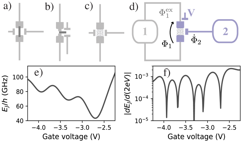
Figure 1: a) Nanowire junction, b) two-dimensional electron gas (2DEG) junction and c) graphene-based Josephson junction. Each semiconducting junction is gated by two voltage lines: one for the dc voltage bias and one to implement the flux-charge interaction. Panels a) and b) are inspired by Ref. Weber (2018). d) Circuit implementation of the flux-charge interaction. e) Approximate graphene junction energy taken from Ref. Wang et al. (2019). f) Magnitude of the first derivative of the Josephson energy in e) with respect to voltage in electronvolts, such that the derivative is dimensionless. (See panels e)-f) for nanowire and 2DEG junctions in Sect. A.6.)

Our approach to implement flux-charge coupling is based on voltage-tunable Josephson junctions Aguado (2020). These junctions can be realized by replacing the usual oxide separating the junction’s superconductors by semiconducting nanowires Larsen et al. (2015); de Lange et al. (2015); Kringhøj et al. (2018); Larsen et al. (2020); Pita-Vidal et al. (2020), two-dimensional electron gases (2DEGs) Casparis et al. (2018); O’Connell Yuan et al. (2021); Hertel et al. (2022); Hazard et al. (2022), or van der Waals materials de Vries et al. (2021); Lee et al. (2015, 2019); Wang et al. (2019); Haque et al. (2021), see Fig. 1a-c). The coupling between the superconductors separated by such barriers is governed by Andreev reflections. The total Andreev bound state (ABS) energy in a multichannel weak-link junction is Larsen et al. (2015)

$$\varepsilon_{J}(V,\Phi_{1})=-\Delta\sum_{i}\sqrt{1-T_{i}(V)\sin^{2}(\pi\Phi_{1}/\Phi_{0})},$$ (1)

where $\Delta$ is the superconducting gap, $T_{i}(V)$ is the transmission probability of channel $i$ which is controlled by the external gate voltage $V$, $\Phi_{1}$ is the gauge-invariant flux across the junction, and $\Phi_{0}=h/(2e)$ is the flux quantum. Here, we focus on the weak transmission limit, $T_{i}(V)\ll 1$, when

$$\varepsilon_{J}(V,\Phi_{1})\approx-E_{J}(V)\cos(2\pi\Phi_{1}/\Phi_{0}),$$ (2)

with the voltage-tunable Josephson coupling $E_{J}(V)=\Delta\sum_{i}T_{i}(V)/4$. The large transmission limit is discussed further in Sect. A.6.

In this work, we propose to couple the weak-link device (1) to a second mode (2) via the gate voltage [see Fig. 1d)] such that the voltage $V$ biasing the weak link is influenced by the voltage across the second mode, $V\to V_{0}+\dot{\Phi}_{2}$, where $V_{0}$ is an external voltage bias and $\dot{\Phi}_{2}$ is the time-derivative of the branch flux of the second mode. In the presence of an external flux $\Phi_{1}^{\mathrm{ex}}$ threading a superconducting loop comprising the junction in Fig. 1d), the charge-flux coupling is revealed by Taylor expanding Eq. 2 in $\Phi_{1(2)}$ about the time-periodic field averages $\langle\Phi_{1(2)}(t)\rangle$

$$\varepsilon_{J}(V_{0}+\dot{\Phi}_{2},\Phi_{1}-\Phi_{1}^{\mathrm{ex}})=\sum_{n,m=0}^{\infty}\frac{\partial^{n+m}\varepsilon_{J}}{\partial V^{n}\partial\Phi_{1}^{m}}\frac{\delta\dot{\Phi}_{2}^{n}\delta\Phi_{1}^{m}}{n!m!},$$ (3)

where $\delta\Phi_{1(2)}=\Phi_{1(2)}-\langle\Phi_{1(2)}(t)\rangle$. Equation 3 leads to an interaction between the voltage of the second mode $\dot{\Phi}_{2}$ and the flux of the first mode $\Phi_{1}$, resulting in a flux-charge interaction in the Hamiltonian describing the device Vool and Devoret (2017).

In the quantized model, $\Phi_{1}$ and $\dot{\Phi}_{2}$ have fluctuations $\propto(\Phi_{0}/2\pi)\sqrt{\pi Z_{1}/R_{Q}}$ and $\propto\omega_{2}(\Phi_{0}/2\pi)\sqrt{\pi Z_{2}/R_{Q}}$ respectively, with $R_{Q}=h/(2e)^{2}\simeq 6.5$ k$\Omega$ the resistance quantum, $Z_{i=(1,2)}$ the impedance of mode $i=(1,2)$, and  $\omega_{2}$ the frequency of the second mode. In what follows we work in the limit $\left|\partial^{n}E_{J}/\partial V^{n}\right|\ll n!\omega_{2}^{1-n}(\pi Z_{2}/R_{Q})^{(1-n)/2}(\Phi_{0}/2\pi)^{1-n}\left|\partial E_{J}/\partial V\right|\leavevmode\nobreak\$ for $n>1$ such that only the first derivative of $E_{J}$ contributes to the interaction Lagrangian and $\sqrt{\pi Z_{1}/R_{Q}}\ll 1$ which is appropriate for a low impedance mode. Under these conditions we truncate Eq. 3 to its first derivative with respect to $V$ and to first order in $\Phi_{1}$ resulting in an interaction Lagrangian of the form [see Sect. A.2 for details]

$$\mathcal{L}_{\mathrm{int}}\approx\frac{G_{21}}{2}\dot{\Phi}_{2}\Phi_{1},$$ (4)

where using Eqs. 2 and 3 the flux-charge coupling strength is

$$G_{21}=\frac{4\pi}{R_{Q}}\frac{E_{J}^{\prime}(V_{0}+\langle\dot{\Phi}_{2}\rangle)}{2e}\sin\left[\frac{2\pi}{\Phi_{0}}(\Phi_{1}^{\mathrm{ex}}-\langle\Phi_{1}(t)\rangle)\right],$$ (5)

where $E_{J}^{\prime}(V)\equiv\partial E_{J}/\partial V$. The flux-charge interaction of Eq. 4 breaks time-reversal symmetry since it is not conserved under the transformation $\dot{\Phi}\to\dot{\Phi}$ and $\Phi\to-\Phi$, and therefore has the form needed to implement nonreciprocal devices Parra-Rodriguez et al. (2019); Rymarz et al. (2021).

The coupling $G_{21}$, which is largest in magnitude at $\Phi_{1}^{\mathrm{ex}}=\pm\Phi_{0}/4$, is generally smaller than $1/R_{Q}=2e/\Phi_{0}$ as suggested by the derivative of the energy dispersion in Fig. 1f) which is obtained from the experimental data of Ref. Wang et al. (2019). By optimizing the device geometry beyond what was done in Ref. Wang et al. (2019), it is possible to increase the electrostatic coupling between the gateline and the semiconducting region of the SNS junction, thereby making $E_{J}^{\prime}/2e$ larger than reported in Fig. 1d). In principle, $G_{21}$ can also be increased using parametric amplification Lemonde et al. (2016); Leroux et al. (2018); Groszkowski et al. (2020). An analysis of the interaction strength based on spectroscopy data for different types of junctions can be found in Sect. A.6. We also note that the leading order effects of the junction nonlinearity are captured by the mean-field approximation of Eq. 5 where the field averages have to be solved for self-consistently.

Here, $E_{J}^{\prime\prime}(V_{0})\langle\dot{\Phi}_{2}\rangle$ is generally much smaller than $E_{J}^{\prime}(V_{0})$ in magnitude, such that $E_{J}^{\prime}(V_{0}+\langle\dot{\Phi}_{2}\rangle)\approx E_{J}^{\prime}(V_{0})$ in Eq. 5. However, for increasing photon numbers in the first mode, the time-average of Eq. 5 decreases in magnitude. Indeed, the averaged flux field in the first mode is $\langle\Phi_{1}(t)\rangle\approx(\Phi_{0}/2\pi)\sqrt{\pi Z_{1}/R_{Q}}\sum_{n=1}^{\infty}\alpha_{1}^{(n)}e^{in\omega t}/\sqrt{2}+\mathrm{h.c}$ with $\alpha_{1}^{(n)}$ the displacement in the $n$th harmonic of the flux field due to an input signal with frequency $\omega$. To leading order in $Z_{1}/R_{Q}\ll 1$, the time-averaged Eq. 5 is then $(4\pi E_{J}^{\prime}/2eR_{Q})\sin(2\pi\Phi_{1}^{\mathrm{ex}}/\Phi_{0})(1-\pi Z_{1}N_{1}/2R_{Q})$ where $N_{1}=\sum_{n=1}^{\infty}|\alpha_{1}^{(n)}|^{2}$ is the photon number in the first mode. As will be explained later, the impedance $Z_{1}$ plays a key role in defining a maximum photon number, $\sim R_{Q}/\pi Z_{1}$, which that can be allowed in the first mode before the FENNEC interaction is impacted by the junction’s nonlinearity. A smaller impedance $Z_{1}$ results in a larger maximum photon number before the interaction is suppressed.

Moreover, at external fluxes where $\sin(2\pi\Phi_{1}^{\mathrm{ex}}/\Phi_{0})=\pm 1$ and $|G_{21}|$ maximized, $G_{12}$ is to first order insensitive to flux noise but sensitive to charge noise proportionally to the second derivative of $E_{J}$ with respect to voltage. However, because $\partial G_{21}/\partial V_{0}$ is orders of magnitude smaller than $G_{12}$, charge and flux noise have negligible effects on the FENNEC interaction strength at those external flux biases. (See Sect. A.4 for details.)

III Gyrator design

The simplest and most fundamental nonreciprocal device based on the flux-charge coupling of Eq. 4 is the gyrator. An ideal gyrator is characterized by the scattering matrix

$$\bm{\mathcal{S}}=\begin{pmatrix}0&1\\ -1&0\end{pmatrix},$$ (6)

which relates the amplitude of the incoming ($\bm{a}$) and outgoing ($\bm{b}$) fields, at each port of the device via $\bm{b}=\bm{S}\cdot\bm{a}$. The circuit Lagrangian of an ideal gyrator takes the form of Parra-Rodriguez et al. (2019); Rymarz et al. (2021)

$$\mathcal{L}_{\mathrm{gyr}}=\frac{G}{2}\left(\dot{\Phi}_{2}\Phi_{1}-\dot{\Phi}_{1}\Phi_{2}\right),$$ (7)

where $G$ is the conductance of the gyrator, $\Phi_{1(2)}$ is the branch flux and $\dot{\Phi}_{1(2)}$ is the voltage at port 1(2).

To realize $\mathcal{L}_{\mathrm{gyr}}$ using the FENNEC interaction, we consider the lumped-element circuit of Fig. 2 comprising two identical internal modes $1$ (blue) and $2$ (green). Each mode contains a symmetric SQUID loop of semiconducting junctions biased at half quantum flux. The FENNEC interaction is realized by capacitively coupling each mode to the voltage port of the other mode’s voltage-tunable junction. The presence of semiconducting junctions in half-quantum-flux-biased SQUIDs results only in the flux-charge interaction without any additional nonlinearity in the inductance of the internal modes of the gyrator. Both modes are also shunted by LC circuits with resonance frequencies setting the central frequency of the device. The flux bias between the LC circuit and the SQUID loop is set to one quarter quantum flux to render the FENNEC interaction quadratic as needed for gyration in Eq. 7. Finally, each internal gyrator mode is coupled to an external port via an inductance. Stray capacitive coupling between the two modes will be mostly present in a realistic implementation and will be briefly analyzed later on when we discuss circuit disorder. We stress that the device, which involves only two modes, is both compact and passive.

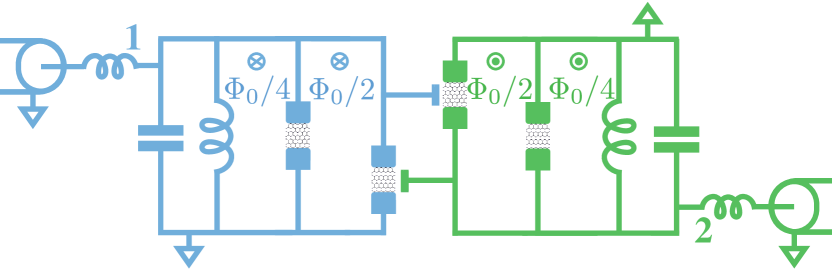
Figure 2: Proposed lumped-element gyrator design. The gyrator is divided in two symmetric subcircuits, shown in blue (left) and green (right). Each half comprises two superconducting loops, where a SQUID of semiconducting junctions is shunted by an inductance $L_{0}$ and a capactiance $C_{0}$. The two junctions have equal superconducting gap $\Delta$ and transmission probabilities $T_{i}(V)$, and are biased at the same dc voltage $V_{0}$. The superconducting loops are threaded by $\pm\Phi_{0}/4$ and $\pm\Phi_{0}/2$, with $+$ ($-$) for the blue (green) half. The two parts are connected through the FENNEC interaction: the branch flux of one subcircuit is coupled to the voltage port of neighboring junction of the other subcircuit. Each subcircuit is connected to an input-output transmission line.

Using Eqs. 4 and 5 with $\Phi_{1}^{\mathrm{ex}}=\Phi_{0}/4$ and $\Phi_{2}^{\mathrm{ex}}=-\Phi_{0}/4$, we find that the circuit of Fig. 2 results in an effective interaction Lagrangian of the form of Eq. 7 with a time-dependent conductance

$$G=\frac{G_{21}-G_{12}}{2}\approx G_{\mathrm{max}}\left[1-\frac{\pi^{2}}{\Phi_{0}^{2}}(\langle\Phi_{1}(t)\rangle^{2}+\langle\Phi_{2}(t)\rangle^{2})\right],$$ (8)

with $G_{21(12)}$ defined in Eq. 5 and

$$G_{\mathrm{max}}=\frac{4\pi}{R_{Q}}\frac{E_{J}^{\prime}(V_{0})}{2e}.$$ (9)

The approximation in Eq. 8 results from Taylor expanding in the field averages $\langle\Phi_{1(2)}(t)\rangle$ to second order and neglecting the second derivative of $E_{J}$ (see Sect. B.4). Typical device parameters (see Fig. 1) result in $G_{\mathrm{max}}\ll 1/R_{Q}$ and therefore a narrow bandwidth. In Eq. 8 the averaged flux field is $\langle\Phi_{1(2)}(t)\rangle\approx(\Phi_{0}/2\pi)\sqrt{\pi Z_{0}/R_{Q}}\sum_{n=1}^{\infty}\alpha_{1(2)}^{(n)}e^{in\omega t}/\sqrt{2}+\mathrm{h.c}$ with $\alpha_{1(2)}^{(n)}$ the displacement in the $n$th harmonic of the flux field due to an input signal with frequency $\omega$, and $Z_{0}=\sqrt{L_{0}/C_{0}}$ the characteristic impedance of the shunting LC. The total photon number in mode $1(2)$ is therefore $N_{1(2)}=\sum_{n=1}^{\infty}|\alpha_{1(2)}^{(n)}|^{2}$. The time-dependent contributions in Eq. 8 result in frequency mixing and, as a consequence, a time-averaged conductance Eq. 8 that decreases from its optimal value with increasing input power. Within the rotating-wave approximation, it is useful to approximate Eq. 8 by its time-average

$$G\approx G_{\mathrm{max}}\left[1-\frac{\pi Z_{0}N}{2R_{Q}}\right]$$ (10)

with $N=(N_{1}+N_{2})/2$ the average photon number in the gyrator which is proportional to the input power. As discussed in further detail below, a reduced conductance leads to increased reflection. The effects of frequency-mixing due to the counter-rotating terms that are dropped in Eq. 8 are analyzed in Sect. B.5.

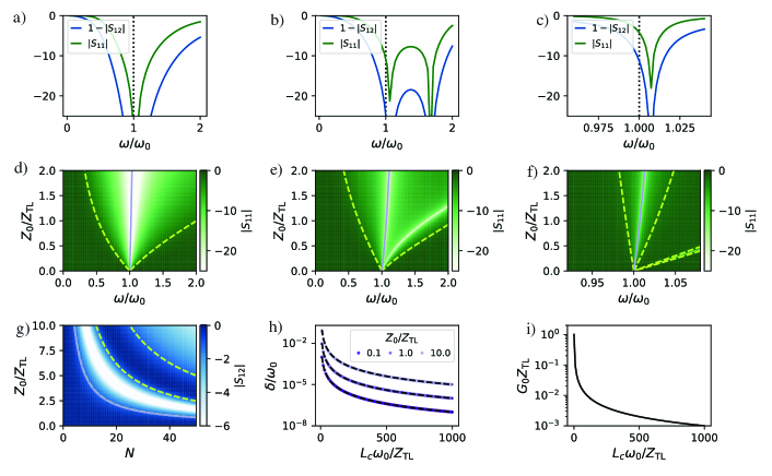
Figure 3: a-c) Reflection $|S_{11}|$ and transmission $|S_{12}|$ in dB computed analytically at the impedance matching condition $G=G_{0}$ as a function of the frequency $\omega$ renormalized by the resonance frequency $\omega_{0}=1/\sqrt{C_{0}L_{0}}$, for different coupling inductances $L_{c}=Z_{\mathrm{TL}}/\omega_{0}\times\{0.05,0.50,5.00\}$ respectively, and for fixed load impedance $Z_{0}=\sqrt{L_{0}/C_{0}}=10Z_{\mathrm{TL}}$ and in the $N=0$ limit. d-f) Two-dimensional version of a-c) where $Z_{0}$ is varied. The dashed lines are the $|\tan(2\theta_{\omega})|=1$ boundaries, where reflection starts to dominate over transmission. Two such boundaries closest to $\omega=\omega_{0}$ are highlighted in light green. The central frequency is identified with a purple line. g) Transmission $|S_{12}|$ versus the photon number $N$ in the gyrator and the load impedance $Z_{0}$. The 1 dB-compression level is highlighted in light green and corresponds to the maximum photon number that can be tolerated in the gyrator. The analytical estimate from Eq. 18 is the purple line which shows agreement with the 1 dB level. h) Numerically computed frequency bandwidth near $\omega=\omega_{0}$ using the boundaries highlighted in d-f) versus the coupling inductance $L_{c}$, for different load impedances $Z_{0}$. The black lines correspond to Eq. 17. Details of the fitting algorithm can be found in Sect. B.5. i) Impedance-matched conductance as a function of coupling inductance $L_{c}$, see Eq. 16.

Scattering matrix. Starting from the equations of motion of the mean-field Lagrangian, we find that the linear scattering response can be expressed as

$$\bm{S}(\omega)=\left(\bm{1}-\frac{\bm{Z_{\omega}}^{-1}}{Z_{\mathrm{TL}}^{-1}}\right)^{-1}\cdot\left(\bm{1}+\frac{\bm{Z_{\omega}}^{-1}}{Z_{\mathrm{TL}}^{-1}}\right),$$ (11)

(see Sect. B.5) where $Z_{\mathrm{TL}}$ is the characteristic impedance of the input-output transmission lines, and $\bm{Z_{\omega}}=i\omega\bm{L_{c}}+[i\omega\bm{C}+(i\omega\bm{L})^{-1}+iG\bm{\sigma_{y}}]^{-1}$ encodes the total impedance of the gyrator modes. Here, $\bm{C}$ and $\bm{L}$ are the $2\times 2$ capacitance and inductance matrices of the gyrator modes respectively, $\bm{\sigma_{y}}$ is the Pauli matrix, and $\bm{L_{c}}$ is the coupling inductance matrix between the transmission lines and the gyrator modes. In the ideal case where $\bm{L_{c}}=L_{c}\bm{1}$, $\bm{C}=C_{0}\bm{1}$ and $\bm{L}=L_{0}\bm{1}$, the scattering matrix reduces to the simple form

$$\bm{S}(\omega)=\cos(2\theta_{\omega})\bm{1}+i\sin(2\theta_{\omega})\bm{\sigma_{y}},$$ (12)

where

$$\tan(2\theta_{\omega})=\frac{2G\overline{Z}_{\mathrm{TL}}(\omega)}{1-\overline{Z}_{\mathrm{TL}}^{2}(\omega)/\overline{Z}_{0}^{2}(\omega)-G^{2}\overline{Z}_{\mathrm{TL}}^{2}(\omega)},$$ (13)

and

$$\overline{Z}_{\mathrm{TL}}(\omega)=\frac{Z_{\mathrm{TL}}}{\left[1+Z_{c}(\omega)/Z_{0}(\omega)\right]^{2}+G^{2}Z_{c}^{2}(\omega)},$$ (14)

$$\overline{Z}_{0}(\omega)=\frac{Z_{0}(\omega)}{1+[Z_{c}(\omega)/Z_{0}(\omega)]\left[1+G^{2}Z_{0}^{2}(\omega)\right]},$$ (15)

are the frequency-dependent characteristic impedance of the lines and renormalized load impedance due to the coupling inductance, respectively. Here $Z_{0}(\omega)=[i\omega C_{0}+(i\omega L_{0})^{-1}]^{-1}$ is the impedance of the load whereas $Z_{c}(\omega)=i\omega L_{c}$ is the impedance of the coupling inductance. $\bm{S}$ approaches the ideal scattering matrix of a gyrator Eq. 6 for $|\tan(2\theta_{\omega})|\to\infty$ or, equivalently, when the circuit is perfectly impedance-matched such that transmission is maximal.

Central frequency. The central frequency of the device corresponds to the frequency for which the denominator in Eq. 13 vanishes with the smallest $G$ possible. As discussed in further details in Sect. B.5, the central frequency is close to the resonance frequency of the internal gyrator modes $\omega_{0}=1/\sqrt{L_{0}C_{0}}$.

Impedance-matched conductance. The conductance for which the scattering matrix approaches that of an ideal gyrator at $\omega=\omega_{0}$ is approximately

$$G_{0}=\overline{Z}_{\mathrm{TL}}(\omega_{0})^{-1}=\frac{\sqrt{1+2\left(\sqrt{2}L_{c}\omega_{0}/Z_{\mathrm{TL}}\right)^{2}}-1}{Z_{\mathrm{TL}}\left(\sqrt{2}L_{c}\omega_{0}/Z_{\mathrm{TL}}\right)^{2}},$$ (16)

which becomes $G_{0}=Z_{\mathrm{TL}}^{-1}$ as $L_{c}\rightarrow 0$. To maximize transmission, we set $G_{\mathrm{max}}$ in Eq. 9 equal to $G_{0}$ in Eq. 16. We also note that $G_{0}$ decreases with increasing $L_{c}$. As will be shown below, we ideally want $L_{c}=0$ such as to maximize the frequency bandwidth of the device leaving us with the constraint $G_{\mathrm{max}}=Z_{\mathrm{TL}}^{-1}$. In cases where the transmission lines have a characteristic impedance $Z_{\mathrm{TL}}\ll G_{\mathrm{max}}^{-1}$, which is most likely for typical circuit parameters, we can nonetheless use a matching circuit between the lines and the gyrator Pozar (2009); Naaman and Aumentado (2022).

Frequency bandwidth. We also introduce the frequency bandwidth $\delta=\omega_{+}-\omega_{-}$ for gyration with $\omega_{\pm}$ the cut-off frequencies for which reflection equals transmission, where $|\tan(2\theta_{\omega})|=1$. At large $L_{c}$, where $G_{0}\approx(L_{c}\omega_{0})^{-1}$, we find (see Sect. B.5)

$$\delta\approx\frac{Z_{0}Z_{\mathrm{TL}}}{L_{c}^{2}\omega_{0}}.$$ (17)

The same expression for zero $L_{c}$ is instead $\delta=2\omega_{0}\sqrt{1+\beta\left(Z_{0}/Z_{\mathrm{TL}}\right)^{2}}$ where $4\beta=G^{2}Z_{\mathrm{TL}}+2|G|Z_{\mathrm{TL}}-1$.

Compression point. As discussed above, frequency mixing can lead to reduced transmission and here we define the compression level as the maximum average photon number $N$ for which the scattering-matrix components deviate by 1 dB from the expected values in the zero-photon linear limit. Near the central frequency $\omega_{0}$ we find that $|\tan(2\theta_{\omega_{0}})|\approx 2(1-x)/[1-(1-x)^{2}]$, where $x=\pi Z_{0}N/2R_{Q}$ using the mean-field expression for the conductance in Eq. 10, see Sect. B.5. From this expression, we find a maximum average photon number

$$N_{\mathrm{max}}\approx\frac{R_{Q}}{\pi Z_{0}}$$ (18)

by setting $|\tan(2\theta_{\omega_{0}})|\approx 1.31$ and with $\theta_{\omega_{0}}$ the angle at which transmission drops by 1 dB in Eq. 12 at the central frequency $\omega_{0}$ with nonzero average photon number $N$. That the maximal photon number $N_{\mathrm{max}}$ decreases with increasing $Z_{0}$ is a signature that the system dynamics is more affected by the junctions nonlinearity for large zero-point fluctuations of the internal gyrator modes. Assuming a typical mode impedance $Z_{0}=50\,\Omega$, Eq. 18 leads to $N_{\mathrm{max}}\approx 41$ photons.

Numerical results. The reflection and transmission coefficients of the scattering matrix in the linear regime (i.e. $N\ll R_{Q}/\pi Z_{0}$) for different $L_{c}$ and $Z_{0}$ are shown in Fig. 3a-f). The frequency bandwidth is shown in Fig. 3h) and the optimal conductance Eq. 16 is shown in Fig. 3i). In panels a-f), we observe that the central frequency (purple line near $\omega_{0}$) slightly deviates from $\omega_{0}$ as a function of $Z_{0}/Z_{\mathrm{TL}}$ for non-zero $L_{c}$ with our choice of conductance $G_{0}$ (see Sect. B.5 for analytical estimates). The dashed light green contours in panels d-f) about $\omega=\omega_{0}$ correspond to $\omega_{\pm}$. We note that the frequency bandwidth near $\omega=\omega_{0}$ also quickly decreases with increasing $L_{c}$, which is clearly illustrated in panel h) where we see excellent agreement with Eq. 17 for large $L_{c}$ values. Panel i) illustrates that the optimal conductance $G_{0}$ is inversely proportional to $L_{c}$. Compression is also shown within mean-field theory in Fig. 3g), with the purple line corresponding to Eq. 18.

Noise sensitivity. The gyrator interaction in Eq. 7 is akin to a Jaynes-Cummings interaction between two resonant LC oscillators that are the internal gyrator modes. This quadratic model, with energy splitting $2G$, is insensitive to both charge and flux noise. Nevertheless, for the design of Fig. 2, and within mean-field theory, the interaction strength given by Eq. 8 is sensitive to both charge noise $\dot{\Phi}_{1(2)}\to\dot{\Phi}_{1(2)}+\delta\dot{\Phi}_{1(2)}$ and flux noise $\Phi_{1(2)}\to\Phi_{1(2)}+\delta\Phi_{1(2)}$. To leading order in the noise, we find that $G\to G+(\partial G_{\mathrm{max}}/\partial V_{0})[\delta\dot{\Phi}_{1}+\delta\dot{\Phi}_{2}]/2$ is insensitive to flux noise but sensitive to charge noise. $\partial G_{\mathrm{max}}/\partial V_{0}\propto E_{J}^{\prime\prime}(V_{0})$ is however orders of magnitude smaller than $G_{\mathrm{max}}$ and consequently charge noise is negligible. Derivations and full analysis for both flux and charge noise can be found in Sect. B.3.

Circuit disorder. Gyration is fragile to frequency mismatches and stray couplings, both unavoidable in realistic circuit implementations and resulting in $\bm{\sigma_{z}}$ and $\bm{\sigma}_{x}$ components in the scattering matrix Eq. 12. We consider $\bm{L_{c}}=L_{c}\bm{1}+dL_{c}\bm{\sigma_{z}}$, $\bm{C}=C_{0}\bm{1}+dC_{0}\bm{\sigma_{z}}-C_{12}\bm{\sigma_{x}}$ and $\bm{L}=L_{0}\bm{1}+dL_{0}\bm{\sigma_{z}}-L_{12}\bm{\sigma_{x}}$ with $dL_{c}$, $dC_{0}$, $dL_{0}$ the disorder in $L_{c}$, $C_{0}$, $L_{0}$, respectively, and $C_{12}$, $L_{12}$ the parasitic capacitive and inductive couplings between active nodes and loops, respectively. As shown in Appendix D, deviations in the scattering matrix elements, proportional to $\bm{\sigma_{z}}$ and $\bm{\sigma_{x}}$, are much smaller than unity for $dL_{c}\ll Z_{\mathrm{TL}}/\omega_{0}$, $dC_{0}\ll Z_{\mathrm{TL}}G_{0}^{2}/\omega_{0}$, $dL_{0}\ll L_{0}^{2}\omega_{0}Z_{\mathrm{TL}}G_{0}^{2}$, $C_{12}\ll Z_{\mathrm{TL}}G_{0}^{2}/\omega_{0}$ and $L_{12}\ll L_{0}^{2}\omega_{0}Z_{\mathrm{TL}}G_{0}^{2}$. These constraints are all realizable in superconducting circuits. We note that a larger optimal conductance $G_{0}$ [i.e. a smaller $L_{c}$ in Eq. 16] renders the device less sensitive to circuit disorder, which is also a direct consequence of a larger frequency bandwidth, see  Eq. 17. Further discussions regarding circuit disorder can be found in Appendix D.

Optimal circuit parameters. Important circuit parameters are the coupling inductance $L_{c}$, the conductance $G_{\mathrm{max}}$ in Eq. 9 which must be set to the optimal conductance value $G_{0}$, and the characteristic impedance $Z_{0}$ of the shunting LC resonators. For typical semiconducting junctions, $G_{\mathrm{max}}\ll Z_{\mathrm{TL}}^{-1}$ which forces $L_{c}$ to be large such that the condition that  $G_{\mathrm{max}}=G_{0}$ can be satisfied accordingly to Eq. 16 unless we use a matching circuit between the transmission lines and the gyrator. A larger $L_{c}$ (i.e. smaller $G_{0}$) results in a smaller frequency bandwidth [see Eq. 17] and increased sensitivity to circuit disorder as noted in the previous paragraph. We also require $Z_{0}\ll R_{Q}$ to maximize Eq. 18 which equally contributes in reducing the frequency bandwidth. Overall the larger $G_{\mathrm{max}}$ can be made the larger the frequency bandwidth and the smallest the sensitivity to circuit disorder.

Beyond mean-field theory. So far we have used the mean-field approach to capture the leading order effects of the circuit nonlinearity in the scattering matrix. However, this approach does not take into account the impact of quantum fluctuations. The time evolution of the full circuit under a dissipative master equation is analyzed in Appendix C, where we show that quantum fluctuations are indeed negligible when comparing reflection against mean-field theory for different input powers and load impedances. In Appendix E, we also follow the circuit-quantization procedure Vool and Devoret (2017) on a generic circuit with the FENNEC interaction which is nonlinear in both the phase and charge quadratures due to the higher derivatives of $E_{J}$. To this end, we introduce a perturbative expansion for the canonical charges with respect to the voltages $\dot{\Phi}_{1}$ and $\dot{\Phi}_{2}$ to take into account the higher derivatives of $E_{J}$. The perturbative expansion yields nonlinear corrections to the quantized circuit Hamiltonian. The leading order effect resulting from the second derivative of $E_{J}$ is a nonlinear capacitive energy that depends on the phase of the other mode.

IV Circulator design

Having demonstrated that the flux-charge interaction leads to the fundamental two-port nonreciprocal element, we use first principles of circuit theory to build more general multi-port devices. As an example, Fig. 4b) shows a symmetric version of a circulator built from the gyrator design of Fig. 2.

The limitations and imperfections of our gyrator design imparted by either the junction nonlinearity or circuit disorder, as discussed in the previous section, will be the same for the circulator design in Fig. 4b). For simplicity, here we therefore consider the gyrator to be ideal. The circulator in Fig. 4b) was already analyzed in Ref. Carlin and Giordano (1964) also considering an ideal gyrator.

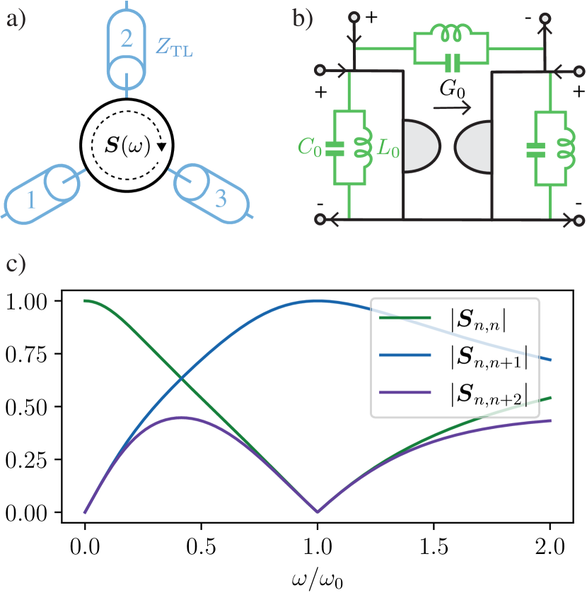
Figure 4: a) Three-port circulator characterized by a scattering matrix $\bm{S}(\omega)$ with input-output transmission lines of impedance $Z_{\mathrm{TL}}$. b) Lumped-element design for a circulator based on a single gyrator with its circuit symbol shown in gray and corresponding to the implementation in Fig. 2. The three equal loads shown in green have a characteristic impedance $Z_{0}$. The gyrator here can be implemented with the FENNEC interaction. c) Absolute values of the full scattering matrix elements versus the frequency for $n=1,2,3$.

In the linear semi-classical regime, i.e. within mean-field theory and for small input photon numbers where FENNEC acts as an ideal gyrator, this device is described by the scattering matrix

$$\bm{S}=\begin{pmatrix}0&1&0\\ 0&0&-1\\ 1&0&0\end{pmatrix},$$ (19)

when the system is probed at resonance ($\omega=\omega_{0}$) and is impedance matched ($Z_{\mathrm{TL}}=Z_{0}=1/G_{0}$). The absolute values of the full scattering matrix elements are shown in Fig. 4c) while details of analytical expressions can be found in Appendix F.

V Conclusion

We proposed a flux-charge interaction that breaks time-reversal symmetry in the presence of static external magnetic fields and which can be used as a building block for passive nonreciprocal devices such as gyrators and circulators. We analytically and numerically investigated the scattering matrix of a gyrator based on the this interaction. The strength of the FENNEC interaction, which we wish to maximize, will determine both the frequency bandwidth of the device and the sensitivity to circuit disorder. The nonlinearity of the junctions will also result in compression similarly to other proposals for circulators Koch et al. (2010); Müller et al. (2018); Richman and Taylor (2021). Despite its narrow bandwidth, the advantages of our gyrator are both its compactness and passiveness.

Beyond applications to nonreciprocal devices, the FENNEC interaction yields either quadratic or nonlinear two-body interactions opening up new possibilities for engineering two-qubit gates and next-generation superconducting qubits Gyenis et al. (2021). Indeed, based on the recent by proposal by Rymarz et al. (2021), it can be shown that GKP states Gottesman et al. (2001) can be stabilized with this interaction et al. .

Appendix A FENNEC interaction properties

A.1 Time-reversal symmetry

Voltages and currents are typically considered even and odd variables with respect to time inversion, i.e. $V(-t)=V(t)$ and $I(-t)=-I(t)$. Given that the fluxes and charges are their time integrals respectively, i.e. $\Phi(t)=\int_{0}^{t}V(\tau)d\tau$ and $Q(t)=\int_{0}^{t}I(\tau)d\tau$, we would then define $\Phi\rightarrow-\Phi$ and $\dot{\Phi}\rightarrow\dot{\Phi}$ under time inversion.

A.2 FENNEC Lagrangian

We consider a generic circuit Lagrangian of the form $\mathcal{L}=\mathcal{L}_{0}+\mathcal{L}_{\mathrm{i}nt}$, where

$$\mathcal{L}_{0}=\dot{\bm{\Phi}}^{T}\cdot\frac{\bm{C_{0}}}{2}\cdot\dot{\bm{\Phi}}+\dot{\bm{\Phi}}^{T}\cdot\frac{\bm{C_{c}}}{2}\cdot\dot{\bm{\Phi}}+\left(\dot{\bm{\Phi}}-\bm{V}\right)^{T}\cdot\frac{\bm{C_{J}}}{2}\cdot\left(\dot{\bm{\Phi}}-\bm{V}\right)-U\left(\bm{\varphi}\right),$$ (20)

is the Lagrangian due to all standard superconducting circuit elements,

$$\begin{split}\mathcal{L}_{\mathrm{i}nt}&=-\varepsilon_{J}(\Delta_{1},\bm{T_{1}},V_{1}+\dot{\Phi}_{2},\varphi_{1}^{\mathrm{ex}},\varphi_{1})=-\sum_{n,m=0}^{\infty}\frac{\dot{\Phi}_{2}^{n}}{n!}\frac{\Phi_{1}^{m}}{m!}\left(\frac{2\pi}{\Phi_{0}}\right)^{m}\frac{\partial^{n+m}\varepsilon_{J}(\Delta_{1},\bm{T_{1}},V_{1},\varphi_{1}^{\mathrm{ex}},0)}{\partial V^{n}\partial\varphi^{m}}\end{split}$$ (21)

results from the FENNEC interaction alone. Here $\bm{\Phi}=\left(\Phi_{1},\ \Phi_{2}\right)$ is a vector comprising the branch flux $\Phi_{1}$ ($\Phi_{2}$) of the first (second) mode, $\bm{\varphi}=2\pi\bm{\Phi}/\Phi_{0}$ are the associated branch phases, $\bm{C_{0}}$ and $\bm{C_{c}}$ are capacitance matrices due to the shunt capacitors and the coupling capacitors respectively, $\bm{C_{J}}$ is the capacitance matrix associated with the coupling to the control voltage lines $\bm{V}$, $U(\bm{\varphi})$ is any additional potential energy of the two modes,

$$\varepsilon_{J}(\Delta,\bm{T},V,\varphi^{\mathrm{ex}},\varphi)=-\Delta\sum_{i}\sqrt{1-[\bm{T}(V)]_{i}\sin^{2}\left(\frac{\varphi-\varphi^{\mathrm{e}x}}{2}\right)},$$ (22)

is the form of the Andreev bound-state energy of any semiconducting junction in the circuit, $\Delta_{k}$ is the gap energy of the $k$th junction with transmissions $[\bm{T_{k}}]_{i}$, $\Phi_{k}^{\mathrm{e}x}$ is an external flux threading the $k$th loop. In this work we focus on the leading order contribution of the interaction Lagrangian

$$\mathcal{L}_{\textit{fennec}}=G\dot{\Phi}_{2}\Phi_{1}/2,$$ (23)

where we defined the amplitudes

$$G=-\frac{4\pi}{\Phi_{0}}\frac{\partial^{2}\varepsilon_{J}(\Delta_{1},\bm{T_{1}},V_{1},\varphi_{1}^{\mathrm{ex}},0)}{\partial V\partial\varphi}=\frac{4\pi}{\Phi_{0}}\frac{\Delta_{1}}{4}\sum_{i}[\bm{T_{1}}(V_{1})]_{i}^{\prime}\sin\left(\varphi_{1}^{\mathrm{e}x}\right)\frac{1+[\bm{T_{1}}(V_{1})]_{i}\sin^{2}\left(\varphi_{1}^{\mathrm{e}x}/2\right)/2}{\sqrt{1-[\bm{T_{1}}(V_{1})]_{i}\sin^{2}\left(\varphi_{1}^{\mathrm{e}x}/2\right)}^{3}}.$$ (24)

In what follows we truncate the interaction Lagrangian to quadratic order,

$$\mathcal{L}_{\mathrm{int}}\approx\frac{c_{2}}{2}\dot{\Phi}_{2}^{2}-\frac{\Phi_{1}^{2}}{2\ell_{1}}+\alpha_{2}\dot{\Phi}_{2}+\beta_{1}\Phi_{1}+\frac{G}{2}\dot{\Phi}_{2}\Phi_{1}$$ (25)

where we defined the charge offset

$$\alpha_{2}=-\frac{\partial\varepsilon_{J}(\Delta_{1},\bm{T_{1}},V_{1},\varphi_{1}^{\mathrm{ex}},0)}{\partial V}=-\sum_{i}\frac{\Delta_{1}[\bm{T_{1}}(V_{1})]_{i}^{\prime}\sin^{2}\left(\varphi_{1}^{\mathrm{e}x}/2\right)/2}{\sqrt{1-[\bm{T_{1}}(V_{1})]_{i}\sin^{2}\left(\varphi_{1}^{\mathrm{e}x}/2\right)}^{3}},$$ (26)

the phase offset

$$\beta_{1}=-\frac{2\pi}{\Phi_{0}}\frac{\partial\varepsilon_{J}(\Delta_{1},\bm{T_{1}},V_{1},\varphi_{1}^{\mathrm{ex}},0)}{\partial\varphi}=\frac{2\pi}{\Phi_{0}}\sum_{i}\frac{\Delta_{1}[\bm{T_{1}}(V_{1})]_{i}\sin(\varphi_{1}^{\mathrm{e}x})/4}{\sqrt{1-[\bm{T_{1}}(V_{1})]_{i}\sin^{2}\left(\varphi_{1}^{\mathrm{e}x}/2\right)}^{3}},$$ (27)

the shift in the capacitance

$$c_{2}=-\frac{\partial^{2}\varepsilon_{J}(\Delta_{1},\bm{T_{1}},V_{1},\varphi_{1}^{\mathrm{ex}},0)}{\partial V^{2}}=-\sum_{i}\frac{\Delta_{1}\sin^{2}\left(\varphi_{1}^{\mathrm{e}x}/2\right)/2}{\sqrt{1-[\bm{T_{1}}(V_{1})]_{i}\sin^{2}\left(\varphi_{1}^{\mathrm{e}x}/2\right)}}\left[[\bm{T_{1}}(V_{1})]_{i}^{\prime\prime}-\frac{([\bm{T_{1}}(V_{1})]_{i})^{2}\sin^{2}\left(\varphi_{1}^{\mathrm{e}x}/2\right)/2}{1-[\bm{T_{1}}(V_{1})]_{i}\sin^{2}\left(\varphi_{1}^{\mathrm{e}x}/2\right)}\right],$$ (28)

and the shift in the inductance

$$\frac{1}{\ell_{1}}=\left(\frac{2\pi}{\Phi_{0}}\right)^{2}\frac{\partial^{2}\varepsilon_{J}(\Delta_{1},\bm{T_{1}},V_{1},\varphi_{1}^{\mathrm{ex}},0)}{\partial\varphi^{2}}=\left(\frac{2\pi}{\Phi_{0}}\right)^{2}\sum_{i}\frac{\Delta_{1}[\bm{T_{1}}(V_{1})]_{i}/4}{\sqrt{1-[\bm{T_{1}}(V_{1})]_{i}\sin^{2}\left(\varphi_{1}^{\mathrm{e}x}/2\right)}^{3}}\left[\cos(\varphi_{1}^{\mathrm{e}x})+[\bm{T_{1}}(V_{1})]_{i}\sin^{4}\left(\varphi_{1}^{\mathrm{e}x}/2\right)\right].$$ (29)

We already advertise that at $\varphi_{1}^{\mathrm{ex}}=\pm\pi/2$, in the weak transmission limit $[\bm{T_{1}}(V_{1})]_{i}\ll 1$ and more generally $|[\bm{T_{1}}(V_{1})]_{i}^{\prime}|,|[\bm{T_{1}}(V_{1})]_{i}^{\prime\prime}|\ll 1$, the shifts $c_{2}$ and $1/\ell_{1}$ are negligible contributions to the capacitance and inductance of modes 2 and 1 respectively.

A.3 Weak transmission limit

We further simplify the system Lagrangian by considering the weak transmission limit $[\bm{T_{1}}(V_{1})]_{i}\ll 1$ where we find that

$$\varepsilon_{J}(\Delta,\bm{T},V,\varphi^{\mathrm{ex}},\varphi)\approx\Delta+\frac{\Delta\sum_{i}[\bm{T_{1}}(V_{1})]_{i}}{4}-\frac{\Delta\sum_{i}[\bm{T_{1}}(V_{1})]_{i}}{4}\cos\left(\varphi-\varphi^{\mathrm{e}x}\right)=\Delta+E_{J}(\Delta,\bm{T},V)-E_{J}(\Delta,\bm{T},V)\cos\left(\varphi-\varphi^{\mathrm{e}x}\right),$$ (30)

where we defined the effective Josephson energy $E_{J}(\Delta,\bm{T},V)=\Delta\sum_{i}[\bm{T_{1}}(V_{1})]_{i}/4$. We consequently find that

$$G\approx\frac{4\pi}{\Phi_{0}}\frac{\partial E_{J}(\Delta_{1},\bm{T_{1}},V_{1})}{\partial V}\sin(\varphi_{1}^{\mathrm{ex}}),$$ (31)

$$\alpha_{2}=-\frac{\partial E_{J}(\Delta_{1},\bm{T_{1}},V_{1})}{\partial V}+\frac{\partial E_{J}(\Delta_{1},\bm{T_{1}},V_{1})}{\partial V}\cos\left(\varphi^{\mathrm{e}x}\right),$$ (32)

$$\beta_{1}=\frac{2\pi}{\Phi_{0}}E_{J}(\Delta_{1},\bm{T_{1}},V_{1})\sin(\varphi_{1}^{\mathrm{ex}}),$$ (33)

$$c_{2}=-\frac{\partial^{2}E_{J}(\Delta_{1},\bm{T_{1}},V_{1})}{\partial V^{2}}+\frac{\partial^{2}E_{J}(\Delta_{1},\bm{T_{1}},V_{1})}{\partial V^{2}}\cos\left(\varphi^{\mathrm{e}x}\right),$$ (34)

$$\frac{1}{\ell_{1}}=\left(\frac{2\pi}{\Phi_{0}}\right)^{2}E_{J}(\Delta_{1},\bm{T_{1}},V_{1})\cos(\varphi_{1}^{\mathrm{ex}}).$$ (35)

In what follows we drop the small shifts $c_{2}$ and $1/\ell_{1}$ for compactness.

A.4 Noise sensitivity

In this section we analyze the noise sensitivity of the device. Notice that given the term $\varepsilon_{J}(\Delta_{1},\bm{T_{1}},V_{1}+\dot{\Phi}_{2},\varphi_{1}^{\mathrm{ex}},\varphi_{1})$, charge noise in the second mode, such that $\dot{\Phi}_{2}\to\dot{\Phi}_{2}+\delta\dot{\Phi}_{2}$, is equivalent to $V_{1}\to V_{1}+\delta\dot{\Phi}_{2}$. Similarly, flux noise in the first mode, such that $\varphi_{1}\to\varphi_{1}+\delta\varphi_{1}$, is equivalent to $\varphi_{1}^{\mathrm{ex}}\to\varphi_{1}^{\mathrm{ex}}-\delta\varphi_{1}$.

Charge noise. In presence of charge noise, which amounts to $V_{1}\to V_{1}+\delta\dot{\Phi}_{2}$ in the FENNEC interaction strength $G$, we find that $G\to G+\delta G$ where

$$\delta G\approx\frac{4\pi}{\Phi_{0}}\frac{\partial^{2}E_{J}(\Delta_{1},\bm{T_{1}},V_{1})}{\partial V^{2}}\sin(\varphi_{1}^{\mathrm{ex}})\delta\dot{\Phi}_{2}$$ (36)

to leading order in the noise.

Flux noise. In presence of flux noise, which can be implemented with $\varphi_{1}^{\mathrm{ex}}\to\varphi_{1}^{\mathrm{ex}}-\delta\varphi_{1}$ in the FENNEC interaction strength $G$, we find that $G\to G+\delta G$ where

$$\delta G\approx-\left(\frac{4\pi}{\Phi_{0}}\right)^{2}\frac{\partial E_{J}(\Delta_{1},\bm{T_{1}},V_{1})}{\partial V}\cos(\varphi_{1}^{\mathrm{ex}})\delta\Phi_{1}.$$ (37)

Resolution of the strength. Another important point is the resolution of the DC gate voltage bias, $\delta V$, which must satisfy

$$\delta V\ll\left|\frac{4\pi}{\Phi_{0}}\frac{\partial^{2}E_{J}(\Delta_{1},\bm{T_{1}},V_{1})}{\partial V^{2}}\sin(\varphi_{1}^{\mathrm{ex}})\right|^{-1}.$$ (38)

A.5 Mean-field theory

In this section we linearized the FENNEC interaction within a mean-field theory approximation:

$$\begin{split}\mathcal{L}_{\mathrm{i}nt}^{\mathrm{mf}}&=-\sum_{n,m=0}^{\infty}\frac{\delta\dot{\Phi}_{2}^{n}}{n!}\frac{\delta\Phi_{1}^{m}}{m!}\left(\frac{2\pi}{\Phi_{0}}\right)^{m}\frac{\partial^{n+m}\varepsilon_{J}(\Delta_{1},\bm{T_{1}},V_{1}+\langle\dot{\Phi}_{2}\rangle,\varphi_{1}^{\mathrm{ex}}-\langle\varphi_{1}\rangle,0)}{\partial V^{n}\partial\varphi^{m}},\end{split}$$ (39)

where $\delta\Phi_{k}=\Phi_{k}-\langle\Phi_{k}\rangle$. The field averages have to be solved self-consistently. To second order in the fluctuations we arrive at the effective interaction Lagrangian

$$\mathcal{L}_{\mathrm{int}}\approx\alpha_{2}(t)\dot{\Phi}_{2}+\beta_{1}(t)\Phi_{1}+G(t)\dot{\Phi}_{2}\Phi_{1}/2,$$ (40)

where we defined

$$G(t)=-\frac{4\pi}{\Phi_{0}}\frac{\partial^{2}\varepsilon_{J}(\Delta_{1},\bm{T_{1}},V_{1}+\langle\dot{\Phi}_{2}\rangle,\varphi_{1}^{\mathrm{ex}}-\langle\varphi_{1}\rangle,0)}{\partial V\partial\varphi},$$ (41)

$$\alpha_{2}(t)=-\frac{\partial\varepsilon_{J}(\Delta_{1},\bm{T_{1}},V_{1}+\langle\dot{\Phi}_{2}\rangle,\varphi_{1}^{\mathrm{ex}}-\langle\varphi_{1}\rangle,0)}{\partial V}-\langle\Phi_{1}\rangle G(t)/2$$ (42)

$$\beta_{1}(t)=-\frac{2\pi}{\Phi_{0}}\frac{\partial\varepsilon_{J}(\Delta_{1},\bm{T_{1}},V_{1}+\langle\dot{\Phi}_{2}\rangle,\varphi_{1}^{\mathrm{ex}}-\langle\varphi_{1}\rangle,0)}{\partial\varphi}-\langle\dot{\Phi}_{2}\rangle G(t)/2.$$ (43)

To quartic order in the flux we find the approximate interaction Lagrangian $\mathcal{L}_{\mathrm{int}}^{\mathrm{mf}}=G(t)\dot{\Phi}_{2}\Phi_{1}$ where

$$\begin{split}G(t)=\frac{4\pi}{\Phi_{0}}\frac{\partial E_{J}(\Delta_{1},\bm{T_{1}},V_{1})}{\partial V}\sin\left(\varphi_{1}^{\mathrm{ex}}\right)\left(1-\frac{\langle\varphi_{1}\rangle^{2}}{2}\right)+\frac{4\pi}{\Phi_{0}}\frac{\partial^{3}E_{J}(\Delta_{1},\bm{T_{1}},V_{1})}{\partial V^{3}}\sin\left(\varphi_{1}^{\mathrm{ex}}\right)\frac{\langle\dot{\Phi}_{2}\rangle^{2}}{2}\\ -\frac{4\pi}{\Phi_{0}}\frac{\partial^{2}E_{J}(\Delta_{1},\bm{T_{1}},V_{1})}{\partial V^{2}}\cos\left(\varphi_{1}^{\mathrm{ex}}\right)\langle\dot{\Phi}_{2}\rangle\langle\varphi_{1}\rangle.\end{split}$$ (44)

We consider the second and third derivatives of $E_{J}$ to be negligible. $R_{Q}=\Phi_{0}/(2e)=h/(2e)^{2}\simeq 6.5$ k$\Omega$ the resistance quantum.

A.6 Estimation of the interaction strength

We remark that, following standard circuit quantization, the FENNEC interaction yields a Hamiltonian term $(g/\hbar)\hat{q}_{2}\hat{\Phi}_{1}$ where $g=8E_{C_{2}}E_{J}^{\prime}(V_{0})/2e$ and $E_{C_{2}}$ isthe charging energy of the second mode.

The Josephson energy $E_{J}$ in the weak transmission limit is estimated from the approximate Gatemon transition energy formula

$$f_{Q}\approx\left(\sqrt{8E_{C}E_{J}}-E_{C}\right)/h,$$ (45)

where $E_{C}$ is the measured charging energy provided in Larsen et al. (2015); Casparis et al. (2018); Wang et al. (2019). We numerically compute the derivative using an interpolated spline that fits the $f_{Q}$ that was experimentally measured. We also numerically confirm that the FENNEC interaction strength is indeed proportional to this derivative in Figs. 5, 6 and 7. Two-dimensional electron gas junction have smoother energy with respect to the gate voltage (see Fig. 6) but generally weaker first derivative. Nanowire junctions can in principle yield larger first derivatives (see Fig. 7) but appear more noisy. Graphene junctions result in both large first derivatives and smooth profiles (see Fig. 5).

We also note that in the regime of a single channel with large transmission $T(V)$ we instead find  $\varepsilon_{J}(V,\Phi_{1})\approx-\Delta|\cos(\pi\Phi_{1}/\Phi_{0})|+(\Delta/2)(T(V)-1)\sin^{2}(\pi\Phi_{1}/\Phi_{0})|\sec(\pi\Phi_{1}/\Phi_{0})|$, which is more sensitive to the external voltage $V$ near half flux quantum. In other words, it is possible to find larger FENNEC interaction strengths by working in the large transmission limit.

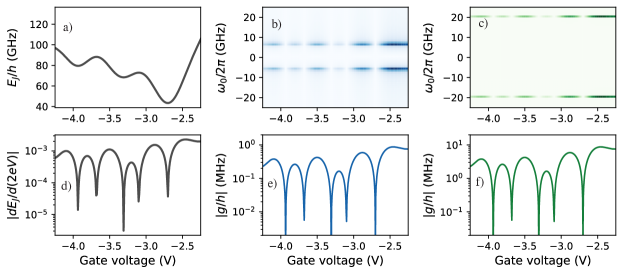
Figure 5: a) Josephson energy estimated from Wang et al. (2019). b)-c) Numerical discrete Fourier transform for different DC gate voltages. Here we add a small AC voltage with frequency and amplitude both determined by the capacitive and inductive energies of a fictitious second mode. The inductive energy is $50/h$ GHz and the capactivie energy is $0.1/h$ GHz in b) and $1.0/h$ GHz in c). d) First derivative of the Josephson energy in a). e)-f) line-cut of b)-c) respectively at the frequency of the AC voltage. e) and f) follow the pattern of the first derivative in d).

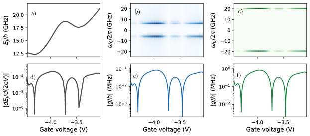
Figure 6: See caption of Fig. 5. Based on the spectroscopy data in Casparis et al. (2018).

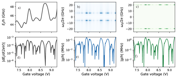
Figure 7: See caption of Fig. 5. Based on the measured gatemon frequency in Larsen et al. (2015).

Appendix B Gyrator implementation

B.1 System Lagrangian

We consider a generic circuit Lagrangian of the form

$$\mathcal{L}=\mathcal{L}_{0}+\mathcal{L}_{\mathrm{i}nt}+\mathcal{L}_{\mathrm{c}or},$$ (46)

where

$$\mathcal{L}_{0}=\dot{\bm{\Phi}}^{T}\cdot\frac{\bm{C_{0}}}{2}\cdot\dot{\bm{\Phi}}+\dot{\bm{\Phi}}^{T}\cdot\frac{\bm{C_{c}}}{2}\cdot\dot{\bm{\Phi}}+\left(\dot{\bm{\Phi}}-\bm{V}\right)^{T}\cdot\frac{\bm{C_{J}}}{2}\cdot\left(\dot{\bm{\Phi}}-\bm{V}\right)-\bm{\Phi}^{T}\cdot\frac{\bm{L_{0}}^{-1}}{2}\cdot\bm{\Phi},$$ (47)

is the Lagrangian due to all standard superconducting circuit elements,

$$\begin{split}\mathcal{L}_{\mathrm{i}nt}&=-\varepsilon_{J}(\Delta_{1},\bm{T_{1}},V_{1}+\dot{\Phi}_{2},\varphi_{1}^{\mathrm{ex}},\varphi_{1})-\varepsilon_{J}(\Delta_{2},\bm{T_{2}},V_{2}+\dot{\Phi}_{1},\varphi_{2}^{\mathrm{ex}},\varphi_{2})\\ &=-\sum_{n,m=0}^{\infty}\frac{\dot{\Phi}_{2}^{n}}{n!}\frac{\Phi_{1}^{m}}{m!}\left(\frac{2\pi}{\Phi_{0}}\right)^{m}\frac{\partial^{n+m}\varepsilon_{J}(\Delta_{1},\bm{T_{1}},V_{1},\varphi_{1}^{\mathrm{ex}},0)}{\partial V^{n}\partial\varphi^{m}}-\sum_{n,m=0}^{\infty}\frac{\dot{\Phi}_{1}^{n}}{n!}\frac{\Phi_{2}^{m}}{m!}\left(\frac{2\pi}{\Phi_{0}}\right)^{m}\frac{\partial^{n+m}\varepsilon_{J}(\Delta_{2},\bm{T_{2}},V_{2},\varphi_{2}^{\mathrm{ex}},0)}{\partial V^{n}\partial\varphi^{m}}\end{split}$$ (48)

results from the FENNEC interaction alone, and

$$\begin{split}\mathcal{L}_{\mathrm{c}or}&=-\varepsilon_{J}(\Delta_{1},\bm{T_{1}},V_{1},\varphi_{1}^{\mathrm{ex}}-\pi,\varphi_{1})-\varepsilon_{J}(\Delta_{2},\bm{T_{2}},V_{2},\varphi_{2}^{\mathrm{ex}}+\pi,\varphi_{2})\\ &=-\sum_{m=0}^{\infty}\frac{\Phi_{1}^{m}}{m!}\left(\frac{2\pi}{\Phi_{0}}\right)^{m}\frac{\partial^{m}\varepsilon_{J}(\Delta_{1},\bm{T_{1}},V_{1},\varphi_{1}^{\mathrm{ex}}-\pi,0)}{\partial\varphi^{m}}-\sum_{m=0}^{\infty}\frac{\Phi_{2}^{m}}{m!}\left(\frac{2\pi}{\Phi_{0}}\right)^{m}\frac{\partial^{m}\varepsilon_{J}(\Delta_{2},\bm{T_{2}},V_{2},\varphi_{2}^{\mathrm{ex}}+\pi,0)}{\partial\varphi^{m}}.\end{split}$$ (49)

will be used to cancel the potentially large interaction-free part of $\mathcal{L}_{\mathrm{int}}$ since $\varepsilon_{J}(\Delta,\bm{T},V,\varphi^{\mathrm{ex}}\pm\pi,0)=-\varepsilon_{J}(\Delta,\bm{T},V,\varphi^{\mathrm{ex}},0)$ in the weak transmission limit $[\bm{T}(V_{1})]_{i}\ll 1$, as will be clear below. Here $\bm{\Phi}=\left(\Phi_{1},\ \Phi_{2}\right)$ is a vector comprising the branch flux $\Phi_{1}$ ($\Phi_{2}$) of the first (second) mode, $\bm{\varphi}=2\pi\bm{\Phi}/\Phi_{0}$ are the associated branch phases, $\bm{C_{0}}$ and $\bm{C_{c}}$ are capacitance matrices due to the shunt capacitors and the coupling capacitors respectively, $\bm{C_{J}}$ is the capacitance matrix associated with the coupling to the control voltage lines $\bm{V}$, $\bm{L_{0}}$ is an inductance matrix,

$$\varepsilon_{J}(\Delta,\bm{T},V,\varphi^{\mathrm{ex}},\varphi)=-\Delta\sum_{i}\sqrt{1-[\bm{T}(V)]_{i}\sin^{2}\left(\frac{\varphi-\varphi^{\mathrm{e}x}}{2}\right)},$$ (50)

is the form of the Andreev bound-state energy of any semiconducting junction in the circuit, $\Delta_{k}$ is the gap energy of the $k$th junction with transmission probability $[\bm{T_{k}}(V_{k})]_{i}$, $\Phi_{k}^{\mathrm{e}x}$ is an external flux threading the $k$th loop. In this work we focus on the leading order contribution of the interaction Lagrangian

$$\mathcal{L}_{\mathrm{target}}=G_{+}(t)\left(\dot{\Phi}_{2}\Phi_{1}+\dot{\Phi}_{1}\Phi_{2}\right)/2+G_{-}(t)\left(\dot{\Phi}_{2}\Phi_{1}-\dot{\Phi}_{1}\Phi_{2}\right)/2,$$ (51)

where we defined the amplitudes

$$G_{\pm}=-\frac{2\pi}{\Phi_{0}}\frac{\partial^{2}\varepsilon_{J}(\Delta_{1},\bm{T_{1}},V_{1},\varphi_{1}^{\mathrm{ex}},0)}{\partial V\partial\varphi}\mp\frac{2\pi}{\Phi_{0}}\frac{\partial^{2}\varepsilon_{J}(\Delta_{2},\bm{T_{2}},V_{2},\varphi_{2}^{\mathrm{ex}},0)}{\partial V\partial\varphi}.$$ (52)

Here

$$\frac{\partial^{2}\varepsilon_{J}(\Delta,\bm{T},V,\varphi^{\mathrm{ex}},0)}{\partial V\partial\varphi}=-\frac{\Delta}{4}\sum_{i}\frac{\partial[\bm{T}(V)]_{i}}{\partial V}\sin\left(\varphi^{\mathrm{e}x}\right)\frac{1-[\bm{T}(V)]_{i}\sin^{2}\left(\varphi^{\mathrm{e}x}/2\right)/2}{\sqrt{1-[\bm{T}(V)]_{i}\sin^{2}\left(\varphi^{\mathrm{e}x}/2\right)}^{3}}.$$ (53)

Moreover $G_{-}(t)=1/(2R)$, where $R$ is the resistance of a gyrator. Overall we truncate the interaction Lagrangian to

$$\mathcal{L}_{\mathrm{int}}+\mathcal{L}_{\mathrm{c}or}\approx\sum_{k=1}^{2}\left[\frac{c_{k}}{2}\dot{\Phi}_{k}^{2}+\frac{\Phi_{k}^{2}}{2\ell_{k}}+\alpha_{k}\dot{\Phi}_{k}+\beta_{k}\Phi_{k}\right]+G_{+}(t)\left(\dot{\Phi}_{2}\Phi_{1}+\dot{\Phi}_{1}\Phi_{2}\right)/2+G_{-}(t)\left(\dot{\Phi}_{2}\Phi_{1}-\dot{\Phi}_{1}\Phi_{2}\right)/2$$ (54)

where we defined

$$c_{k}=-\frac{\partial^{2}\varepsilon_{J}(\Delta_{\ell},\bm{T_{\ell}},V_{\ell},\varphi_{\ell}^{\mathrm{ex}},0)}{\partial V^{2}},$$ (55)

$$\frac{1}{\ell_{k}}=-\left(\frac{2\pi}{\Phi_{0}}\right)^{2}\frac{\partial^{2}\varepsilon_{J}(\Delta_{k},\bm{T_{k}},V_{k},\varphi_{k}^{\mathrm{ex}},0)}{\partial\varphi^{2}}-\left(\frac{2\pi}{\Phi_{0}}\right)^{2}\frac{\partial^{2}\varepsilon_{J}(\Delta_{k},\bm{T_{k}},V_{k},\varphi_{k}^{\mathrm{ex}}+(-1)^{k}\pi,0)}{\partial\varphi^{2}},$$ (56)

$$\alpha_{k}=-\frac{\partial\varepsilon_{J}(\Delta_{\ell},\bm{T_{\ell}},V_{\ell},\varphi_{\ell}^{\mathrm{ex}},0)}{\partial V},$$ (57)

$$\beta_{k}=-\frac{2\pi}{\Phi_{0}}\frac{\partial\varepsilon_{J}(\Delta_{k},\bm{T_{k}},V_{k},\varphi_{k}^{\mathrm{ex}},0)}{\partial\varphi}-\frac{2\pi}{\Phi_{0}}\frac{\partial\varepsilon_{J}(\Delta_{k},\bm{T_{k}},V_{k},\varphi_{k}^{\mathrm{ex}}+(-1)^{k}\pi,0)}{\partial\varphi}.$$ (58)

For optimal gyration we wish for $G_{-}(t)$ ($G_{+}(t)$) to be maximized (minimized). $G_{-}(t)$ leads to a resonant Jaynes-Cummings-type interaction with a $\pi/2$ relative phase ($i\hat{a}^{\dagger}\hat{b}+\mathrm{h.c}$) whereas $G_{+}(t)$ leads to a off-resonant two-mode-squeezing-type interaction ($i\hat{a}^{\dagger}\hat{b}^{\dagger}+\mathrm{h.c}$).

B.2 Weak transmission limit

In the weak transmission ($[\bm{T_{k}}(V_{k})]_{i}\ll 1$) limit we find that

$$\varepsilon_{J}(\Delta,\bm{T},V,\varphi^{\mathrm{ex}},\varphi)\approx\Delta+\frac{\Delta\sum_{i}[\bm{T}(V)]_{i}}{4}-\frac{\Delta\sum_{i}[\bm{T}(V)]_{i}}{4}\cos\left(\varphi-\varphi^{\mathrm{e}x}\right)=\Delta+E_{J}(\Delta,\bm{T},V)-E_{J}(\Delta,\bm{T},V)\cos\left(\varphi-\varphi^{\mathrm{e}x}\right).$$ (59)

Notice that

$$c_{k}=-\left(1-\cos\left(\varphi_{\ell}^{\mathrm{ex}}\right)\right)\frac{\partial^{2}E_{J}(\Delta_{\ell},\bm{T_{\ell}},V_{\ell})}{\partial V^{2}},$$ (60)

$$\frac{1}{\ell_{k}}=0,$$ (61)

$$\alpha_{k}=-\left(1-\cos\left(\varphi_{\ell}^{\mathrm{ex}}\right)\right)\frac{\partial E_{J}(\Delta_{\ell},\bm{T_{\ell}},V_{\ell})}{\partial V},$$ (62)

$$\beta_{k}=0.$$ (63)

From now on we will drop $c_{k}$ and $1/\ell_{k}$ in the assumption that they are negligible contributions to the capacitance and inductance of the modes.

Gyration.

If the FENNEC interaction can prove useful for two-qubit gates the main application is the realization of nonreciprocal devices. It follows that

$$G_{-}(t)\approx\frac{\pi}{R_{Q}}\sin\left(\varphi_{1}^{\mathrm{e}x}\right)\frac{1}{2e}\frac{\partial E_{J}(\Delta_{1},\bm{T_{1}},V_{1})}{\partial V}-\frac{\pi}{R_{Q}}\sin\left(\varphi_{2}^{\mathrm{e}x}\right)\frac{1}{2e}\frac{\partial E_{J}(\Delta_{2},\bm{T_{2}},V_{2})}{\partial V}$$ (64)

where we defined $R_{Q}=\Phi_{0}/(2e)=h/(2e)^{2}\simeq 6.5$ k$\Omega$ the resistance quantum. Importantly, this implies that the resistance of the gyrator is

$$R=\frac{R_{Q}}{2\pi}\left(\sin\left(\varphi_{1}^{\mathrm{e}x}\right)\frac{1}{2e}\frac{\partial E_{J}(\Delta_{1},\bm{T_{1}},V_{1})}{\partial V}-\sin\left(\varphi_{2}^{\mathrm{e}x}\right)\frac{1}{2e}\frac{\partial E_{J}(\Delta_{2},\bm{T_{2}},V_{2})}{\partial V}\right)^{-1}.$$ (65)

Typically $|\partial E_{J}(\Delta_{k},\bm{T_{k}},V_{k})/\partial V|\ll 1$ and it is therefore clear that the resistance of the gyrator $R$ is mostly likely larger than the resistance quantum $R_{Q}$.

B.3 Noise sensitivity

In this section we analyze the noise sensitivity of the device. Notice that given the term $\varepsilon_{J}(\Delta_{1},\bm{T_{1}},V_{1}+\dot{\Phi}_{2},\varphi_{1}^{\mathrm{ex}},\varphi_{1})$, charge noise in the second mode, such that $\dot{\Phi}_{2}\to\dot{\Phi}_{2}+\delta\dot{\Phi}_{2}$, is equivalent to $V_{1}\to V_{1}+\delta\dot{\Phi}_{2}$. Similarly, flux noise in the first mode, such that $\varphi_{1}\to\varphi_{1}+\delta\varphi_{1}$, is equivalent to $\varphi_{1}^{\mathrm{ex}}\to\varphi_{1}^{\mathrm{ex}}-\delta\varphi_{1}$.

Charge noise. In presence of charge noise, which amounts to $V_{1}\to V_{1}+\delta\dot{\Phi}_{2}$ and  $V_{2}\to V_{2}+\delta\dot{\Phi}_{1}$ in the FENNEC interaction strength $G_{-}(t)$, we find that $G_{-}(t)\to G_{-}(t)+\delta G_{-}(t)$ where

$$\delta G_{-}(t)\approx\frac{\pi}{R_{Q}}\sin\left(\varphi_{1}^{\mathrm{e}x}\right)\frac{1}{2e}\frac{\partial^{2}E_{J}(\Delta_{1},\bm{T_{1}},V_{1})}{\partial V^{2}}\delta\dot{\Phi}_{2}-\frac{\pi}{R_{Q}}\sin\left(\varphi_{2}^{\mathrm{e}x}\right)\frac{1}{2e}\frac{\partial^{2}E_{J}(\Delta_{2},\bm{T_{2}},V_{2})}{\partial V^{2}}\delta\dot{\Phi}_{1}$$ (66)

to leading order in the noise.

The frequencies of the normal modes of gyrator become $\omega_{\pm}=\omega_{0}\pm G_{-}(t)\pm\delta G_{-}(t)$. We observe that the dispersion is linear in charge noise and determined by the second derivative of $E_{J}$.

Flux noise. In presence of flux noise, which can be implemented with $\varphi_{1}^{\mathrm{ex}}\to\varphi_{1}^{\mathrm{ex}}-\delta\varphi_{1}$ and  $\varphi_{2}^{\mathrm{ex}}\to\varphi_{2}^{\mathrm{ex}}-\delta\varphi_{2}$ in the FENNEC interaction strength $G_{-}(t)$, we find that $G_{-}(t)\to G_{-}(t)+\delta G_{-}(t)$ where

$$\delta G_{-}(t)\approx-\frac{\pi}{R_{Q}}\cos\left(\varphi_{1}^{\mathrm{e}x}\right)\frac{1}{2e}\frac{\partial E_{J}(\Delta_{1},\bm{T_{1}},V_{1})}{\partial V}\delta\varphi_{1}+\frac{\pi}{R_{Q}}\cos\left(\varphi_{2}^{\mathrm{e}x}\right)\frac{1}{2e}\frac{\partial E_{J}(\Delta_{2},\bm{T_{2}},V_{2})}{\partial V}\delta\varphi_{2}.$$ (67)

We observe that the system is insensitive to flux noise to leading order at the optimal gyration point $|\varphi_{k}^{\mathrm{ex}}|=\pi/2$.

B.4 Mean-field theory

In this section we linearized the FENNEC interaction within a mean-field theory approximation:

$$\begin{split}\mathcal{L}_{\mathrm{i}nt}^{\mathrm{mf}}&=-\varepsilon_{J}(\Delta_{1},\bm{T_{1}},V_{1}+\dot{\Phi}_{2},\varphi_{1}^{\mathrm{ex}},\varphi_{1})-\varepsilon_{J}(\Delta_{2},\bm{T_{2}},V_{2}+\dot{\Phi}_{1},\varphi_{2}^{\mathrm{ex}},\varphi_{2})\\ &=-\sum_{n,m=0}^{\infty}\frac{\delta\dot{\Phi}_{2}^{n}}{n!}\frac{\delta\Phi_{1}^{m}}{m!}\left(\frac{2\pi}{\Phi_{0}}\right)^{m}\frac{\partial^{n+m}\varepsilon_{J}(\Delta_{1},\bm{T_{1}},V_{1}+\langle\dot{\Phi}_{2}\rangle,\varphi_{1}^{\mathrm{ex}}-\langle\varphi_{1}\rangle,0)}{\partial V^{n}\partial\varphi^{m}}\\ &-\sum_{n,m=0}^{\infty}\frac{\delta\dot{\Phi}_{1}^{n}}{n!}\frac{\delta\Phi_{2}^{m}}{m!}\left(\frac{2\pi}{\Phi_{0}}\right)^{m}\frac{\partial^{n+m}\varepsilon_{J}(\Delta_{2},\bm{T_{2}},V_{2}+\langle\dot{\Phi}_{1}\rangle,\varphi_{2}^{\mathrm{ex}}-\langle\varphi_{2}\rangle,0)}{\partial V^{n}\partial\varphi^{m}},\end{split}$$ (68)

where $\delta\Phi_{k}=\Phi_{k}-\langle\Phi_{k}\rangle$. Similarly,

$$\begin{split}\mathcal{L}_{\mathrm{c}or}^{\mathrm{mf}}&=-\varepsilon_{J}(\Delta_{1},\bm{T_{1}},V_{1}+\dot{\Phi}_{2},\varphi_{1}^{\mathrm{ex}}-\pi,\varphi_{1})-\varepsilon_{J}(\Delta_{2},\bm{T_{2}},V_{2}+\dot{\Phi}_{1},\varphi_{2}^{\mathrm{ex}}+\pi,\varphi_{2})\\ &=-\sum_{m=0}^{\infty}\frac{\delta\Phi_{1}^{m}}{m!}\left(\frac{2\pi}{\Phi_{0}}\right)^{m}\frac{\partial^{m}\varepsilon_{J}(\Delta_{1},\bm{T_{1}},V_{1},\varphi_{1}^{\mathrm{ex}}-\pi-\langle\varphi_{1}\rangle,0)}{\partial\varphi^{m}}\\ &-\sum_{m=0}^{\infty}\frac{\delta\Phi_{2}^{m}}{m!}\left(\frac{2\pi}{\Phi_{0}}\right)^{m}\frac{\partial^{m}\varepsilon_{J}(\Delta_{2},\bm{T_{2}},V_{2},\varphi_{2}^{\mathrm{ex}}+\pi-\langle\varphi_{2}\rangle,0)}{\partial\varphi^{m}}.\end{split}$$ (69)

To second order we therefore arrive at the effective interaction Lagrangian

$$\mathcal{L}_{\mathrm{int}}^{\mathrm{mf}}+\mathcal{L}_{\mathrm{cor}}^{\mathrm{mf}}\approx\sum_{k=1}^{2}\left[\alpha_{k}(t)\dot{\Phi}_{k}+\beta_{k}(t)\Phi_{k}\right]+G_{+}(t)\left(\dot{\Phi}_{2}\Phi_{1}+\dot{\Phi}_{1}\Phi_{2}\right)/2+G_{-}(t)\left(\dot{\Phi}_{2}\Phi_{1}-\dot{\Phi}_{1}\Phi_{2}\right)/2,$$ (70)

where we defined

$$G_{\pm}(t)=-\frac{2\pi}{\Phi_{0}}\frac{\partial^{2}\varepsilon_{J}(\Delta_{1},\bm{T_{1}},V_{1}+\langle\dot{\Phi}_{2}\rangle,\varphi_{1}^{\mathrm{ex}}-\langle\varphi_{1}\rangle,0)}{\partial V\partial\varphi}\mp\frac{2\pi}{\Phi_{0}}\frac{\partial^{2}\varepsilon_{J}(\Delta_{2},\bm{T_{2}},V_{2}+\langle\dot{\Phi}_{1}\rangle,\varphi_{2}^{\mathrm{ex}}-\langle\varphi_{2}\rangle,0)}{\partial V\partial\varphi},$$ (71)

$$\alpha_{k}(t)=-\frac{\partial\varepsilon_{J}(\Delta_{\ell},\bm{T_{\ell}},V_{\ell}+\langle\dot{\Phi}_{k}\rangle,\varphi_{\ell}^{\mathrm{ex}}-\langle\varphi_{\ell}\rangle,0)}{\partial V}-\langle\Phi_{\ell}\rangle\frac{G_{+}(t)+(-1)^{\ell}G_{-}(t)}{4},$$ (72)

$$\beta_{k}(t)=-\frac{2\pi}{\Phi_{0}}\frac{\partial\varepsilon_{J}(\Delta_{k},\bm{T_{k}},V_{k}+\langle\dot{\Phi}_{\ell}\rangle,\varphi_{k}^{\mathrm{ex}}-\langle\varphi_{k}\rangle,0)}{\partial\varphi}-\frac{2\pi}{\Phi_{0}}\frac{\partial\varepsilon_{J}(\Delta_{k},\bm{T_{k}},V_{k},\varphi_{k}^{\mathrm{ex}}+(-1)^{k}\pi-\langle\varphi_{k}\rangle,0)}{\partial\varphi}$$

$$\phantom{\beta_{k}(t)=}-\langle\dot{\Phi}_{\ell}\rangle\frac{G_{+}(t)+(-1)^{\ell}G_{-}(t)}{4},$$ (73)

where $\ell\neq k$. The field averages have to be solved self-consistently. To quartic order in the flux while neglecting higher order derivatives in either $V$ or $\varphi$, we find that

$$G_{\pm}(t)=\frac{2\pi}{\Phi_{0}}\frac{\partial E_{J}(\Delta_{1},\bm{T_{1}},V_{1})}{\partial V}\sin\left(\varphi_{1}^{\mathrm{ex}}\right)\left(1-\frac{\langle\varphi_{1}\rangle^{2}}{2}\right)\pm\frac{2\pi}{\Phi_{0}}\frac{\partial E_{J}(\Delta_{2},\bm{T_{2}},V_{2})}{\partial V}\sin\left(\varphi_{2}^{\mathrm{ex}}\right)\left(1-\frac{\langle\varphi_{2}\rangle^{2}}{2}\right)$$ (74)

$$\alpha_{k}(t)=-\left(1-\cos(\varphi_{\ell}^{\mathrm{ex}})\right)\frac{\partial E_{J}(\Delta_{\ell},\bm{T_{\ell}},V_{\ell})}{\partial V},$$ (75)

and $\beta_{k}(t)=0$.

B.5 Scattering matrix of the linearized system

In this section, we focus on the linear mean-field Lagrangian Hazard et al. (2019):

$$\begin{split}\mathcal{L}^{\mathrm{mf}}=\sum_{i=1}^{2}\int_{-\infty}^{0}dx\left[\frac{c}{2}\left(\partial_{t}\tilde{\Phi}_{i}(x,t)\right)^{2}-\frac{1}{2\ell}\left(\partial_{x}\tilde{\Phi}_{i}(x,t)\right)^{2}\right]-\left(\bm{\tilde{\Phi}}(0,t)-\bm{\Phi}\right)^{T}\cdot\frac{\bm{L_{c}}^{-1}}{2}\cdot\left(\bm{\tilde{\Phi}}(0,t)-\bm{\Phi}\right)+\bm{\alpha}^{T}\cdot\dot{\bm{\Phi}}\\ +\dot{\bm{\Phi}}^{T}\cdot\frac{\bm{C}}{2}\cdot\dot{\bm{\Phi}}-\bm{\Phi}^{T}\cdot\frac{\bm{L}^{-1}}{2}\cdot\bm{\Phi}+\dot{\bm{\Phi}}^{T}\cdot\frac{G_{+}(t)\bm{\sigma_{x}}-iG_{-}(t)\bm{\sigma_{y}}}{4}\cdot\bm{\Phi}+\bm{\Phi}^{T}\cdot\frac{G_{+}(t)\bm{\sigma_{x}}+iG_{-}(t)\bm{\sigma_{y}}}{4}\cdot\dot{\bm{\Phi}},\end{split}$$ (76)

where $\bm{L_{c}}$ is assumed to be diagonal. Here $\bm{\sigma_{x}}$ and $\bm{\sigma_{y}}$ are the Pauli matrices.

Equations of motion

The equations of motion for the effectively linearized Lagrangian are given by

$$0=\partial_{t}\frac{\partial\mathcal{L}^{\mathrm{mf}}}{\partial(\partial_{t}\tilde{\Phi}_{i})}+\partial_{x}\frac{\partial\mathcal{L}^{\mathrm{mf}}}{\partial(\partial_{x}\tilde{\Phi}_{i})}-\frac{\partial\mathcal{L}^{\mathrm{mf}}}{\partial\tilde{\Phi}_{i}}=\frac{d}{dt}\frac{\partial\mathcal{L}^{\mathrm{mf}}}{\partial\dot{\Phi}_{i}}-\frac{\partial\mathcal{L}^{\mathrm{mf}}}{\partial\Phi_{i}},\quad i=1,2,$$ (77)

which explicitly take the form

$$c\partial_{t}^{2}\bm{\tilde{\Phi}}(x,t)=\frac{1}{\ell}\partial_{x}^{2}\bm{\tilde{\Phi}}(x,t),$$ (78)

$$\frac{1}{\ell}\partial_{x}\bm{\tilde{\Phi}}(0,t)=\bm{L_{c}}^{-1}\cdot\left(\bm{\tilde{\Phi}}(0,t)-\bm{\Phi}\right),$$ (79)

$$0=\bm{C}\cdot\ddot{\bm{\Phi}}+\bm{L}^{-1}\cdot\bm{\Phi}-iG_{-}(t)\bm{\sigma_{y}}\cdot\dot{\bm{\Phi}}-\frac{1}{\ell}\partial_{x}\bm{\tilde{\Phi}}(0,t).$$ (80)

Given the wave-equation Eq. 78 we find that the quantized field in the transmission line $j$ has the form

$$\bm{\tilde{\Phi}}(x,t)=\sqrt{\frac{\hbar}{4\pi c}}\int_{0}^{\infty}\frac{d\omega}{\sqrt{\omega}}\left(e^{i\omega t+ik_{\omega}x}\bm{a_{\omega}}^{\dagger}+e^{i\omega t-ik_{\omega}x}\bm{b}_{\omega}^{\dagger}+\mathrm{h.c.}\right),$$ (81)

with the dispersion relation $k_{\omega}=\omega\sqrt{c\hskip 1.00006pt\ell}=\omega/\omega_{\mathrm{TL}}$ and commutation relations $\left[\hat{a}_{i,\omega},\hat{a}_{j,\omega^{\prime}}^{\dagger}\right]=\delta_{ij}\delta(\omega-\omega^{\prime})$ and $\left[\hat{b}_{i,\omega},\hat{b}_{j,\omega^{\prime}}^{\dagger}\right]=\delta_{ij}\delta(\omega-\omega^{\prime})$. Here $\bm{a_{\omega}}$ ($\bm{b_{\omega}}$) are the annihilation operators associated with the ingoing (outgoing) fields at frequency $\omega$.

Fourier transform

We apply a Fourier transform on Eqs. 79 and 80 (with the definition $\hat{y}(\omega)=\int_{-\infty}^{\infty}dt\ y(t)e^{i\omega t}/\sqrt{2\pi}$ and property $y(-\omega)=[y(\omega)]^{*}$):

$$\bm{\hat{\Phi}}(\omega)=\bm{\hat{\tilde{\Phi}}}(0,\omega)-\frac{\bm{L_{c}}}{\ell}\cdot\partial_{x}\bm{\hat{\tilde{\Phi}}}(0,\omega),$$ (82)

$$0=\left(-\omega^{2}\bm{C}+\bm{L}^{-1}\right)\cdot\bm{\hat{\Phi}}(\omega)-\int_{-\infty}^{\infty}d\omega^{\prime}\ \omega^{\prime}\hat{G}_{-}(\omega-\omega^{\prime})\bm{\sigma_{y}}\cdot\bm{\hat{\Phi}}(\omega^{\prime})-\frac{1}{\ell}\partial_{x}\bm{\hat{\tilde{\Phi}}}(0,\omega).$$ (83)

Expansion in the amplitude of the flux fields

$G_{-}(t)$ depends on the average of the flux fields which we assume to have small amplitude. We write $G_{-}(t)=\overline{G}_{-}+\lambda dG_{-}(t)$ where

$$\overline{G}_{-}=\frac{2\pi}{\Phi_{0}}\frac{\partial E_{J}(\Delta_{1},\bm{T}1,V_{1})}{\partial V}\sin\left(\varphi_{1}^{\mathrm{ex}}\right)-\frac{2\pi}{\Phi_{0}}\frac{\partial E_{J}(\Delta_{2},\bm{T_{2}},V_{2})}{\partial V}\sin\left(\varphi_{2}^{\mathrm{ex}}\right)$$ (84)

is the contribution that is independent of the flux fields, and

$$\begin{split}\lambda dG_{-}(t)&=\frac{2\pi}{\Phi_{0}}\frac{\partial E_{J}(\Delta_{2},\bm{T_{2}},V_{2})}{\partial V}\sin\left(\varphi_{2}^{\mathrm{ex}}\right)\frac{\langle\varphi_{2}(t)\rangle^{2}}{2}-\frac{2\pi}{\Phi_{0}}\frac{\partial E_{J}(\Delta_{1},\bm{T_{1}},V_{1})}{\partial V}\sin\left(\varphi_{1}^{\mathrm{ex}}\right)\frac{\langle\varphi_{1}(t)\rangle^{2}}{2}\end{split},$$ (85)

depends on the flux fields following the mean-field approximation. We do a perturbative expansion in $\lambda$, i.e. $\hat{\bm{\tilde{\Phi}}}(0,\omega)=\sum_{k=0}^{\infty}\lambda^{k}\hat{\bm{\tilde{\Phi}}}^{(k)}(0,\omega)$ and $\lambda dG_{-}(t)=\sum_{k=0}^{\infty}\lambda^{k+1}dG_{-}^{(k)}(t)$, and solve Eq. 83 in each order of $\lambda$. For conciseness we stop at first order.

Order 0:

$$0=\left(-\omega^{2}\bm{C}+\bm{L}^{-1}-\omega\overline{G}_{-}\bm{\sigma_{y}}\right)\cdot\left(\bm{\hat{\tilde{\Phi}}}^{(0)}(0,\omega)-\frac{\bm{L_{c}}}{\ell}\cdot\partial_{x}\bm{\hat{\tilde{\Phi}}}^{(0)}(0,\omega)\right)-\frac{1}{\ell}\partial_{x}\bm{\hat{\tilde{\Phi}}}^{(0)}(0,\omega).$$ (86)

Order 1:

$$\begin{split}0=\left(-\omega^{2}\bm{C}+\bm{L}^{-1}-\omega\overline{G}_{-}\bm{\sigma_{y}}\right)\cdot\left(\bm{\hat{\tilde{\Phi}}}^{(1)}(0,\omega)-\frac{\bm{L_{c}}}{\ell}\cdot\partial_{x}\bm{\hat{\tilde{\Phi}}}^{(1)}(0,\omega)\right)-\frac{1}{\ell}\partial_{x}\bm{\hat{\tilde{\Phi}}}^{(1)}(0,\omega)\\ -\int_{-\infty}^{\infty}d\omega^{\prime}\ \omega^{\prime}\hat{dG}_{-}^{(0)}(\omega-\omega^{\prime})\bm{\sigma_{y}}\cdot\left(\bm{\hat{\tilde{\Phi}}}^{(0)}(0,\omega^{\prime})-\frac{\bm{L_{c}}}{\ell}\cdot\partial_{x}\bm{\hat{\tilde{\Phi}}}^{(0)}(0,\omega^{\prime})\right).\end{split}$$ (87)

Consistently with the perturbative expansion we have that

$$\begin{split}\lambda dG_{-}^{0}(t)&=\frac{2\pi}{\Phi_{0}}\frac{\partial E_{J}(\Delta_{2},\bm{T_{2}},V_{2})}{\partial V}\sin\left(\varphi_{2}^{\mathrm{ex}}\right)\frac{\langle\varphi_{2}^{(0)}(t)\rangle^{2}}{2}-\frac{2\pi}{\Phi_{0}}\frac{\partial E_{J}(\Delta_{1},\bm{T_{1}},V_{1})}{\partial V}\sin\left(\varphi_{1}^{\mathrm{ex}}\right)\frac{\langle\varphi_{1}^{(0)}(t)\rangle^{2}}{2}\end{split}.$$ (88)

Input/output equations

Accordingly to Eq. 81 we have in the case $\omega>0$

$$\bm{\hat{\tilde{\Phi}}}^{(k)}(x,\omega>0)=\sqrt{\frac{\hbar}{4\pi c\omega}}\left(e^{-ik_{\omega}x}\bm{a_{\omega}}\delta_{k,0}+e^{ik_{\omega}x}\bm{b_{\omega}}^{(k)}\right),$$ (89)

where $\delta_{ij}=\begin{cases}1,&i=j\\ 0,&i\neq j\end{cases}$ is the discrete delta function. Eq. 86 then takes the form

$$0=\bm{a_{\omega}}+\bm{b_{\omega}}^{(0)}+\frac{\bm{Z}(\omega)}{Z_{\mathrm{TL}}}\cdot\left(\bm{a_{\omega}}-\bm{b_{\omega}}^{(0)}\right)$$ (90)

where $Z_{\mathrm{TL}}=\sqrt{\ell/c}$ is the characteristic impedance of the transmission lines and

$$\bm{Z}(\omega)=i\omega\bm{L_{c}}+\left(i\omega\bm{C}+(i\omega\bm{L})^{-1}+i\overline{G}_{-}\bm{\sigma_{y}}\right)^{-1}=i\omega\bm{L_{c}}+\bm{Z_{0}}(\omega).$$ (91)

At zeroth order the scattering matrix is then

$$\bm{b_{\omega}}^{(0)}=\bm{S}^{(0)}(\omega)\cdot\bm{a_{\omega}}=\left(\frac{\bm{Z}(\omega)}{Z_{\mathrm{TL}}}-1\right)^{-1}\cdot\left(\frac{\bm{Z}(\omega)}{Z_{\mathrm{TL}}}+1\right)\cdot\bm{a_{\omega}}.$$ (92)

Similarly we observe that Eq. 87 reduces to

$$\bm{b_{\omega}}^{(1)}=\int_{-\infty}^{\infty}d\omega^{\prime}\ \frac{\omega^{\prime}}{\omega}Z_{\mathrm{TL}}\hat{dG}_{-}^{(0)}(\omega-\omega^{\prime})\left(\frac{\bm{Z}(\omega^{\prime})}{Z_{\mathrm{TL}}}-1\right)^{-1}\cdot\frac{\bm{Z_{0}}(\omega^{\prime})}{Z_{\mathrm{TL}}}\cdot i2\bm{\sigma_{y}}\cdot\left(\frac{\bm{Z}(\omega^{\prime})}{Z_{\mathrm{TL}}}-1\right)^{-1}\cdot\frac{\bm{Z_{0}}(\omega^{\prime})}{Z_{\mathrm{TL}}}\cdot\bm{a_{\omega^{\prime}}},$$ (93)

using the identities

$$1+\bm{S}^{(0)}(\omega)=2\left(\frac{\bm{Z}(\omega)}{Z_{\mathrm{TL}}}-1\right)^{-1}\cdot\frac{\bm{Z}(\omega)}{Z_{\mathrm{TL}}}\quad\textrm{and}\quad 1-\bm{S}^{(0)}(\omega)=-2\left(\frac{\bm{Z}(\omega)}{Z_{\mathrm{TL}}}-1\right)^{-1}.$$ (94)

Next we must solve for $dG_{-}^{(0)}(t)$. Eq. 82 yields, for $\omega>0$,

$$\bm{\hat{\Phi}}^{(0)}(\omega)=\sqrt{\frac{\hbar}{4\pi c\omega}}\left(\bm{a_{\omega}}+\bm{b_{\omega}}^{(0)}+\frac{i\omega\bm{L_{c}}}{Z_{\mathrm{TL}}}\cdot\left(\bm{a_{\omega}}-\bm{b_{\omega}}^{(0)}\right)\right)=\sqrt{\frac{\hbar}{\pi c\omega}}\left(\frac{\bm{Z}(\omega)}{Z_{\mathrm{TL}}}-1\right)^{-1}\frac{\bm{Z_{0}}(\omega)}{Z_{\mathrm{TL}}}\cdot\bm{a_{\omega}},$$ (95)

Monotonic incoming field

In what follows we assume that the incoming field is monotonic with frequency $\omega_{0}$. As a result we find that

$$\begin{split}\langle\bm{\varphi}(t)\rangle^{2}&=\chi\left(\frac{\bm{Z}^{\dagger}(\omega_{0})}{Z_{\mathrm{TL}}}-1\right)^{-1}\frac{\bm{Z_{0}}^{\dagger}(\omega_{0})}{Z_{\mathrm{TL}}}\cdot|\langle\bm{a_{\omega_{0}}}\rangle|^{2}\cdot\frac{\bm{Z_{0}}(\omega_{0})}{Z_{\mathrm{TL}}}\cdot\left(\frac{\bm{Z}(\omega_{0})}{Z_{\mathrm{TL}}}-1\right)^{-1}\\ &+\frac{\chi}{2}\left(\frac{\bm{Z}^{T}(\omega_{0})}{Z_{\mathrm{TL}}}-1\right)^{-1}\frac{\bm{Z_{0}}^{T}(\omega_{0})}{Z_{\mathrm{TL}}}\cdot\langle\bm{a_{\omega_{0}}}\rangle^{2}\cdot\frac{\bm{Z_{0}}(\omega_{0})}{Z_{\mathrm{TL}}}\cdot\left(\frac{\bm{Z}(\omega_{0})}{Z_{\mathrm{TL}}}-1\right)^{-1}e^{-i2\omega_{0}t}+\mathrm{h.c.},\end{split}$$ (96)

where we defined the quantity

$$\chi=\left(\frac{2\pi}{\Phi_{0}}\right)^{2}\frac{2\hbar}{\pi c\omega}=\frac{4}{R_{Q}c\omega}$$ (97)

Now we observe that

$$\hat{dG}_{-}^{(0)}(\omega)=\hat{dG}_{-}^{(0)}(0)\delta(\omega)+\hat{dG}_{-}^{(0)}(2\omega_{0})\delta(\omega-\omega_{0})+\hat{dG}_{-}^{(0)}(-2\omega_{0})\delta(\omega+\omega_{0}),$$ (98)

in other words, $\hat{dG}_{-}^{(0)}(\omega)$ is sharply peaked at three frequencies. The $\omega=0$ component leads to compression, and under conservation of total exctations, $\omega=\pm 2\omega_{0}$ lead to frequency mixing. Indeed, the outgoing fields are no longer monotonic as they oscillate at both $\omega_{0}$ and $3\omega_{0}$, the latter having much smaller amplitude. Importantly we see that the scattering matrix is rectangular:

$$\begin{pmatrix}\bm{b_{-3\omega_{0}}}\\ \bm{b_{-\omega_{0}}}\\ \bm{b_{+\omega_{0}}}\\ \bm{b_{+3\omega_{0}}}\end{pmatrix}=\begin{pmatrix}\bm{M}(-3\omega_{0};-\omega_{0})&\bm{0}\\ \bm{S}^{(0)}(-\omega_{0})&\bm{M}(-\omega_{0};+\omega_{0})\\ \bm{M}(+\omega_{0};-\omega_{0})&\bm{S}^{(0)}(+\omega_{0})\\ \bm{0}&\bm{M}(+3\omega_{0};+\omega_{0})\end{pmatrix}\cdot\begin{pmatrix}\bm{a_{-\omega_{0}}}\\ \bm{a_{+\omega_{0}}}\end{pmatrix}$$ (99)

where we defined the frequency-mixing matrices

$$\bm{M}(\omega;\omega^{\prime})=\frac{\omega^{\prime}}{\omega}Z_{\mathrm{TL}}\hat{dG}_{-}^{(0)}(\omega-\omega^{\prime})\left(\frac{\bm{Z}(\omega^{\prime})}{Z_{\mathrm{TL}}}-1\right)^{-1}\cdot\frac{\bm{Z_{0}}(\omega^{\prime})}{Z_{\mathrm{TL}}}\cdot i2\bm{\sigma_{y}}\cdot\left(\frac{\bm{Z}(\omega^{\prime})}{Z_{\mathrm{TL}}}-1\right)^{-1}\cdot\frac{\bm{Z_{0}}(\omega^{\prime})}{Z_{\mathrm{TL}}},$$ (100)

which are ultimately proportional to $\chi$.

Effective linear response theory

The leading order effect of the nonlinearity is compression: frequency mixing can be thought as its direct consequence. Compression is associated with the static component of $dG_{-}(t)$ only. We therefore propose an effective linear response theory that captures compression:

$$\bm{b_{\omega}}\simeq\bm{S}(\omega)\cdot\bm{a_{\omega}}=\left(\frac{\bm{Z}(\omega)}{Z_{\mathrm{TL}}}-1\right)^{-1}\cdot\left(\frac{\bm{Z}(\omega)}{Z_{\mathrm{TL}}}+1\right)\cdot\bm{a_{\omega}},$$ (101)

where

$$\bm{Z}(\omega)=i\omega\bm{L_{c}}+\left(i\omega\bm{C}+(i\omega\bm{L})^{-1}+iG\bm{\sigma_{y}}\right)^{-1},$$ (102)

$$G=\overline{G}_{-}+\lambda\hat{dG}_{-}^{0}(0)=\frac{2\pi}{\Phi_{0}}\frac{\partial E_{J}(\Delta_{1},\bm{T_{1}},V_{1})}{\partial V}\sin\left(\varphi_{1}^{\mathrm{ex}}\right)\left(1-\frac{\pi Z_{0}N_{1}}{2R_{Q}}\right)-\frac{2\pi}{\Phi_{0}}\frac{\partial E_{J}(\Delta_{2},\bm{T_{2}},V_{2})}{\partial V}\sin\left(\varphi_{2}^{\mathrm{ex}}\right)\left(1-\frac{\pi Z_{0}N_{2}}{2R_{Q}}\right),$$ (103)

with $N_{1(2)}$ the average photon number in the internal gyrator mode $1(2)$ with characteristic impedance $Z_{0}$. It can be verified that Taylor expanding Eq. 101 to leading order in $\lambda\hat{dG}_{-}^{0}(0)$ returns the linear part of Eq. 93.

Ideal case.

We consider the limiting case $\bm{L_{c}}=L_{c}\bm{1}$, $\bm{C}=C_{0}\bm{1}$ and $\bm{L}=L_{0}\bm{1}$. In this case we find that

$$\frac{\bm{Z}(\omega)}{Z_{\mathrm{TL}}}=\frac{Z_{c}(\omega)}{Z_{\mathrm{TL}}}\bm{1}+\frac{\left(Z_{0}^{-1}(\omega)\bm{1}+iG\bm{\sigma_{y}}\right)^{-1}}{Z_{\mathrm{TL}}}=\frac{Z_{c}(\omega)}{Z_{\mathrm{TL}}}\bm{1}+\frac{Z_{\mathrm{TL}}/Z_{0}(\omega)}{(Z_{\mathrm{TL}}/Z_{0}(\omega))^{2}+G^{2}Z_{\mathrm{TL}}^{2}}\bm{1}-\frac{iGZ_{\mathrm{TL}}}{(Z_{\mathrm{TL}}/Z_{0}(\omega))^{2}+G^{2}Z_{\mathrm{TL}}^{2}}\bm{\sigma_{y}},$$ (104)

where $Z_{0}(\omega)=\left(i\omega C_{0}+(i\omega L_{0})^{-1}\right)^{-1}$ is the load impedance and $Z_{c}(\omega)=i\omega L_{c}$ is the impedance associated with the coupling inductance. Our goal will be to redefine $Z_{0}(\omega)$ and $Z_{\mathrm{TL}}$ such as to include $L_{c}$. To this end consider

$$\frac{\bm{Z}(\omega)}{Z_{\mathrm{TL}}}=\frac{\left(\overline{Z}_{0}^{-1}(\omega)\bm{1}+iG\bm{\sigma_{y}}\right)^{-1}}{\overline{Z}_{\mathrm{TL}}(\omega)}=\frac{\overline{Z}_{\mathrm{TL}}(\omega)/\overline{Z}_{0}(\omega)}{(\overline{Z}_{\mathrm{TL}}(\omega)/\overline{Z}_{0}(\omega))^{2}+G^{2}\overline{Z}_{\mathrm{TL}}^{2}(\omega)}\bm{1}-\frac{iG\overline{Z}_{\mathrm{TL}}(\omega)}{(\overline{Z}_{\mathrm{TL}}(\omega)/\overline{Z}_{0}(\omega))^{2}+G^{2}\overline{Z}_{\mathrm{TL}}^{2}(\omega)}\bm{\sigma_{y}}.$$ (105)

By putting the last two equations equal we find the effective load impedance due to the coupling inductance

$$\overline{Z}_{0}(\omega)=\frac{Z_{0}(\omega)}{1+(Z_{c}(\omega)/Z_{0}(\omega))(1+G^{2}Z_{0}^{2}(\omega))},$$ (106)

and the effective frequency-dependent characteristic impedance of the lines

$$\overline{Z}_{\mathrm{TL}}(\omega)=\frac{Z_{\mathrm{TL}}}{\left(1+Z_{c}(\omega)/Z_{0}(\omega)\right)^{2}+G^{2}Z_{c}^{2}(\omega)}.$$ (107)

With these definitions we find that

$$\left(\frac{\bm{Z}(\omega)}{Z_{\mathrm{TL}}}-1\right)^{-1}\cdot\left(\frac{\bm{Z}(\omega)}{Z_{\mathrm{TL}}}+1\right)=\frac{((a-1)\bm{1}-ib\bm{\sigma_{y}})\cdot((a+1)\bm{1}+ib\bm{\sigma_{y}})}{(a-1)^{2}+b^{2}}=\frac{(a^{2}+b^{2}-1)\bm{1}-i2b\bm{\sigma_{y}}}{(a-1)^{2}+b^{2}},$$ (108)

where $\bm{Z}(\omega)=a\bm{1}+ib\bm{\sigma_{y}}$ with

$$a=\frac{\overline{Z}_{\mathrm{TL}}(\omega)/\overline{Z}_{0}(\omega)}{(\overline{Z}_{\mathrm{TL}}(\omega)/\overline{Z}_{0}(\omega))^{2}+G^{2}\overline{Z}_{\mathrm{TL}}^{2}(\omega)},$$ (109)

$$b=-\frac{G\overline{Z}_{\mathrm{TL}}(\omega)}{(\overline{Z}_{\mathrm{TL}}(\omega)/\overline{Z}_{0}(\omega))^{2}+G^{2}\overline{Z}_{\mathrm{TL}}^{2}(\omega)}.$$ (110)

We therefore find that the scattering matrix reduces to

$$\bm{S}(\omega)=\cos(2\theta_{\omega})\bm{1}+i\sin(2\theta_{\omega})\bm{\sigma_{y}}$$ (111)

where we defined the angle $\theta_{\omega}$ via

$$\tan(2\theta_{\omega})=\frac{2G\overline{Z}_{\mathrm{TL}}(\omega)}{1-\overline{Z}_{\mathrm{TL}}^{2}(\omega)/\overline{Z}_{0}^{2}(\omega)-G^{2}\overline{Z}_{\mathrm{TL}}^{2}(\omega)}.$$ (112)

Central frequency.

The central frequency $\omega_{0}^{\prime}$ of the device corresponds to the frequency for which the denominator in Eq. 112 vanishes, i.e.

$$G^{2}=\overline{Z}_{\mathrm{TL}}^{-2}(\omega_{0}^{\prime})-\overline{Z}_{0}^{-2}(\omega_{0}^{\prime}).$$ (113)

Moreover we wish for the optimal conductance $G$ to be minimized, i.e. $\overline{Z}_{\mathrm{TL}}^{2}(\omega_{0}^{\prime})/\overline{Z}_{0}^{2}(\omega_{0}^{\prime})\to 0$ and $G=1/\overline{Z}_{\mathrm{TL}}(\omega_{0}^{\prime})$. Naturally we wish for both $\overline{Z}_{\mathrm{TL}}(\omega_{0}^{\prime})$ and $\overline{Z}_{0}(\omega_{0}^{\prime})$ to be large. $\omega_{0}^{\prime}$ must therefore be the frequency at which $\overline{Z}_{\mathrm{TL}}(\omega_{0}^{\prime})$ peaks. Using $G=1/\overline{Z}_{\mathrm{TL}}(\omega_{0}^{\prime})$ we find that Eq. 107 becomes

$$0=Z_{c}^{2}(\omega_{0}^{\prime})\overline{Z}_{\mathrm{TL}}^{-2}(\omega_{0}^{\prime})-Z_{\mathrm{TL}}\overline{Z}_{\mathrm{TL}}^{-1}(\omega_{0}^{\prime})+\left(1+Z_{c}(\omega_{0}^{\prime})/Z_{0}(\omega_{0}^{\prime})\right)^{2},$$ (114)

which reduces to

$$\overline{Z}_{\mathrm{TL}}^{-1}(\omega_{0}^{\prime})=\frac{Z_{\mathrm{TL}}}{2Z_{c}^{2}(\omega_{0}^{\prime})}\left(1-\sqrt{1-\frac{4Z_{c}^{2}(\omega_{0}^{\prime})}{Z_{\mathrm{TL}}^{2}}\left(1+\frac{Z_{c}(\omega_{0}^{\prime})}{Z_{0}(\omega_{0}^{\prime})}\right)^{2}}\right),$$ (115)

where $Z_{c}^{2}(\omega_{0}^{\prime})<0$.

We would like to minimize $|\overline{Z}_{\mathrm{TL}}^{-1}(\omega_{0}^{\prime})|$ such as to maximize $|\overline{Z}_{\mathrm{TL}}(\omega_{0}^{\prime})|$. We find a root at $\omega_{0}^{\prime}/\omega_{0}=\sqrt{1+Z_{0}/L_{c}\omega_{0}}$. However this is not sufficient to define the central frequency. Indeed, we notice that for $L_{c}\to 0$, $|\overline{Z}_{\mathrm{TL}}^{-1}(\omega_{0}^{\prime})|=Z_{\mathrm{TL}}^{-1}$ is flat meaning that it cannot be minimized. This leads us to also consider the second condition that $\overline{Z}_{0}^{-1}(\omega_{0}^{\prime})=0$ to satisfy Eq. 113:

$$0=Z_{0}^{-1}(\omega_{0}^{\prime})+Z_{c}(\omega_{0}^{\prime})Z_{0}^{-2}(\omega_{0}^{\prime})+Z_{c}(\omega_{0}^{\prime})\overline{Z}_{\mathrm{TL}}^{-2}(\omega_{0}^{\prime}).$$ (116)

We quickly observe that for $L_{c}=0$, thus $Z_{c}(\omega_{0}^{\prime})=0$, we exactly find $\omega_{0}^{\prime}=\omega_{0}$. For large $L_{c}$, such that $\overline{Z}_{\mathrm{TL}}^{-1}(\omega_{0}^{\prime})\approx-iZ_{0}^{-1}(\omega_{0}^{\prime})$, we still find $\omega_{0}^{\prime}\approx\omega_{0}$.

In what follows we therefore approximate $\omega_{0}^{\prime}\approx\omega_{0}$ to compute optimal parameters for gyration such as the conductance $G\approx 1/\overline{Z}_{\mathrm{TL}}(\omega_{0})$. Because of this approximation we emphasize that in the end the central frequency will be found by numerically solving Eq. 113.

However for an arbitrary $G$, solving $\overline{Z}_{\mathrm{TL}}^{-2}(\omega)-\overline{Z}_{0}^{-2}(\omega)-G^{2}=0$ reveals that

$$\frac{\omega_{c}}{\omega_{0}}-1\approx\frac{\overline{Z}_{\mathrm{TL}}^{-2}(\omega_{0})-G^{2}+G^{4}L_{c}^{2}\omega_{0}^{2}}{2G^{2}(2L_{c}\omega_{0}/Z_{0}-G^{2}L_{c}^{2}\omega_{0}^{2})+4Z_{\mathrm{TL}}^{-2}(1-G^{2}L_{c}^{2}\omega_{0}^{2})(2L_{c}\omega_{0}/Z_{0}+G^{2}L_{c}^{2}\omega_{0}^{2})}.$$ (117)

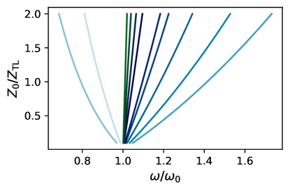
Figure 8: Central frequency obtained by numerically solving for the root of Eq. 116 along with Eq. 115 from $L_{c}\omega_{0}/Z_{\mathrm{TL}}=0.05$ (dark blue) to $L_{c}\omega_{0}/Z_{\mathrm{TL}}=50.00$ (dark green).

Optimal conductance.

$|\tan(2\theta_{\omega})|\to\infty$ corresponds to perfect gyration where $\bm{S}$ resembles Eq. 6. This occurs at central frequency, where the denominator of Eq. 112 vanishes, which we found to be

$$\omega_{0}^{\prime}\approx\omega_{0}=1/\sqrt{L_{0}C_{0}}.$$ (118)

This is approximately where $G$ can take on a minimal value (assuming $\overline{Z}_{\mathrm{TL}}^{2}(\omega_{0})/\overline{Z}_{0}^{2}(\omega_{0})\approx 0$)

$$G_{0}=Z_{\mathrm{TL}}^{-1}\left(\sqrt{1+2x^{2}}-1\right)/x^{2},\quad x=\sqrt{2}\omega_{0}^{\prime}L_{c}/Z_{\mathrm{TL}},$$ (119)

such $G_{0}=\overline{Z}_{\mathrm{TL}}(\omega_{0})^{-1}$ and therefore $|\tan(2\theta_{\omega})|\to\infty$. The approximation we make in this work is $\omega_{0}^{\prime}\approx\omega_{0}$ in Eq. 119.

Frequency bandwidth.

We define the frequency bandwidth $\Delta=\omega_{+}-\omega_{-}$ for gyration with the cut-off frequencies $\omega_{\pm}$ for which reflection equals transmission, i.e. when $|\tan(2\theta_{\omega})|=1$. We consider two limiting cases: $L_{c}=0$ and $L_{c}\gg 0$.

• $L_{c}=0$. For $\theta_{\omega}=\pm\pi/8$ solve the equation

  $$1+|Z_{\mathrm{TL}}/Z_{0}(\omega)|^{2}-G^{2}Z_{\mathrm{TL}}^{2}\mp 2GZ_{\mathrm{TL}}=0$$ (120)

  according to Eq. 112. Here we observe that this equation can only be valid if $\mp G<0$ at perfect impedance matching where $GZ_{\mathrm{TL}}=1$. We therefore simplify the equation to

  $$1+|Z_{\mathrm{TL}}/Z_{0}(\omega)|^{2}-G^{2}Z_{\mathrm{TL}}^{2}-2|G|Z_{\mathrm{TL}}=0\ \rightarrow\ Z_{\mathrm{TL}}/Z_{0}(\omega)=\pm i\sqrt{G^{2}Z_{\mathrm{TL}}^{2}+2|G|Z_{\mathrm{TL}}-1}=\pm i2\epsilon.$$ (121)

  We finally arrive at the explicit constraint

  $$(\omega/\omega_{0})^{2}\pm(2\epsilon Z_{0}/Z_{\mathrm{TL}})(\omega/\omega_{0})-1=0,$$ (122)

  where $Z_{0}=\sqrt{L_{0}/C_{0}}$ is the impedance of the load. We find the solutions

  $$\frac{\omega_{\pm}}{\omega_{0}}=\frac{\epsilon Z_{0}}{Z_{\mathrm{TL}}}\pm\sqrt{1+\left(\frac{\epsilon Z_{0}}{Z_{\mathrm{TL}}}\right)^{2}}.$$ (123)

  We finally find the frequency bandwidth

  $$\frac{\omega_{+}-\omega_{-}}{\omega_{0}}=2\sqrt{1+\left(\frac{\epsilon Z_{0}}{Z_{\mathrm{TL}}}\right)^{2}}.$$ (124)

• $L_{c}\gg 0$. As a simplification we focus on perfect impedance matching, i.e. we choose $G$ such that $\left|G\overline{Z}_{\mathrm{TL}}(\omega_{0})\right|=1$, which corresponds to $G=1/L_{c}\omega_{0}$ according to Eq. 119 in the large $L_{c}$ limit. As seen in Fig. 9a)-b) we find that $\overline{Z}_{0}(\omega)\approx\left(G^{2}Z_{c}(\omega_{0})Z_{\mathrm{TL}}\right)^{-1}$ and $\overline{Z}_{\mathrm{TL}}(\omega)\approx Z_{0}(\omega)Z_{\mathrm{TL}}/2Z_{c}(\omega_{0})$ in the large $Z_{0}(\omega)$ limit and for $G^{2}Z_{c}^{2}(\omega_{0})\approx-1$. We also observe that $\overline{Z}_{\mathrm{TL}}^{2}(\omega)/\overline{Z}_{0}^{2}(\omega)\approx-1$. This fact allows us to approximate

  $$\tan(2\theta_{\omega})\approx 2G\overline{Z}_{\mathrm{TL}}(\omega),$$ (125)

  which shows near perfect agreement in Fig. 9c) near $\omega=\omega_{0}$. We also emphasize that the $|\tan(2\theta_{\omega})|=1$ condition occurs in a range smaller than the frequency range plotted here. We are ultimately interested in finding frequencies for which $|\tan(2\theta_{\omega})|=1$ closest to $\omega_{0}$. Eq. 125 indicates that this occurs for

  $$\left|2G\overline{Z}_{\mathrm{TL}}(\omega)\right|=1.$$ (126)

  Finally we find the approximate constraint

  $$\frac{\omega_{0}}{\omega}-\frac{\omega}{\omega_{0}}=\pm\frac{Z_{0}Z_{\mathrm{TL}}}{L_{c}^{2}\omega_{0}^{2}},$$ (127)

  where we used $Z_{0}(\omega)=iZ_{0}\left(\omega_{0}/\omega-\omega/\omega_{0}\right)^{-1}\approx(iZ_{0}/2)(1-\omega/\omega_{0})^{-1}$ to leading order in $\omega-\omega_{0}$. This leads to the cut-off frequencies

  $$\frac{\omega_{\pm}}{\omega_{0}}=\sqrt{\left(\frac{Z_{0}Z_{\mathrm{TL}}}{2L_{c}^{2}\omega_{0}^{2}}\right)^{2}+1}\pm\frac{Z_{0}Z_{\mathrm{TL}}}{2L_{c}^{2}\omega_{0}^{2}}\approx 1\pm\frac{Z_{0}Z_{\mathrm{TL}}}{2L_{c}^{2}\omega_{0}^{2}}.$$ (128)

  Finally we find the frequency bandwidth

  $$\frac{\omega_{+}-\omega_{-}}{\omega_{0}}\approx\frac{Z_{0}Z_{\mathrm{TL}}}{L_{c}^{2}\omega_{0}^{2}}.$$ (129)

  

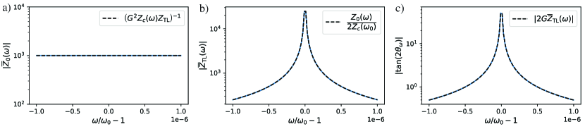
  Figure 9: Analytical estimates in presence of a coupling inductance.

Compression level.

At central frequency we find that $|\tan(2\theta_{\omega_{0}})|\approx 2(1-x)/(1-(1-x)^{2})$ where $x=\pi Z_{0}N/2R_{Q}$ and $N=\zeta_{1}N_{1}+\zeta_{2}N_{2}$ given that $|G_{0}\overline{Z}_{\mathrm{TL}}(\omega_{0})|=1$ for perfect impedance matching at $N_{1}=N_{2}=0$ and $G=G_{0}(1-x)$, and where $\zeta_{1(2)}$ are determined from Eq. 103. For identical junctions and flux biases satisfying $\sin(\varphi_{1}^{\mathrm{ex}})=-\sin(\varphi_{2}^{\mathrm{ex}})$ we find that $\zeta_{1}=\zeta_{2}=1/2$. When transmission drops by 1 dB such that $|\sin(2\theta_{\omega_{0}})|=10^{-0.1}$ and therefore reflection is $|\cos(2\theta_{\omega_{0}})|=\sqrt{1-10^{-0.2}}$, we find that $\left|\tan(2\theta_{\omega})\right|=10^{-0.1}/\sqrt{1-10^{-0.2}}$. We therefore find the constraint

$$\frac{10^{-0.1}}{\sqrt{1-10^{-0.2}}}=\frac{2(1-x)}{1-(1-x)^{2}},\quad x=\pi Z_{0}N/2R_{Q}.$$ (130)

We obtain the maximum average photon number

$$N_{\mathrm{max}}=\frac{R_{Q}}{\pi Z_{0}}.$$ (131)

Numerics

Dimensionless parameters.

It is useful to define the following dimensionless quantities:

• Renormalized frequency:

  $$\omega^{\prime}=\omega/\omega_{0}$$

  where $\omega_{0}=1/\sqrt{L_{0}C_{0}}$ is the central frequency.

• Renormalized coupling inductance:

  $$L_{c}^{\prime}=L_{c}\omega_{0}/Z_{\mathrm{TL}}$$

  where $Z_{\mathrm{TL}}$ is the characteristic impedance of the transmission lines.

• Renormalized characteristic impedance of the load:

  $$Z_{0}^{\prime}=Z_{0}/Z_{\mathrm{TL}}$$

  where $Z_{0}=\sqrt{L_{0}/C_{0}}$ is the characteristic impedance of the load.

• Renormalized conductance: $G^{\prime}=GZ_{\mathrm{TL}}$ where $G$ is the conductance of the gyrator.

The system can therefore be entirely characterized by three parameters $L_{C}^{\prime}$, $Z_{0}^{\prime}$ and $G^{\prime}$ to be optimized. Here $\omega_{0}$ and $Z_{\mathrm{TL}}$ are parameters to be defined.

Frequency bandwidth

We numerically solve for when Eq. 112 is $\pm\pi/8$ using the least_squares algorithm in Scipy. The distance between the two solutions closest to $\omega_{0}$ is used to defined the bandwidth. The solutions are shown in Fig. 10a) for different $L_{c}$’s with corresponding residuals plotted in b). The frequency bandwidth is then shown in c) and compared against the analytical estimate in Eq. 129 (black lines). We observe near perfect quantitative agreement in the large $L_{c}$ limit.

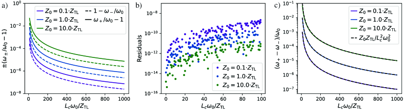
Figure 10: Numerical computation of the frequency bandwidth. a) Cut-off frequencies $\omega_{\pm}$ for which $|\tan(2\theta_{\omega})|=\pi/8$ for different $L_{c}$’s, closest to $\omega_{0}$. b) Residuals of the least_squares algorithm in scipy. c) Frequency bandwidth obtained from a) and compared against Eq. 129.

Appendix C System Hamiltonian and Effective Lindblad Master equation

C.1 Canonical quantization

We consider the gyrator Lagrangian in Eq. 46 and add transmission lines interacting with internal gyrator modes via a coupling inductance as in Eq. 76. We stop at the first derivative of the junctions’ transmission coefficients.

The canonical charge fields are

$$\tilde{q}_{1}(x,t)=\frac{\partial\mathcal{L}}{\partial(\partial_{t}\tilde{\Phi}_{1}(x,t))}=c\partial_{t}\Phi_{1}(x,t),\quad\tilde{q}_{2}(x,t)=\frac{\partial\mathcal{L}}{\partial(\partial_{t}\tilde{\Phi}_{1}(x,t))}=c\partial_{t}\Phi_{2}(x,t),$$ (132)

while the canonical charges are

$$q_{1}=C_{0}\dot{\Phi}_{1}-\frac{\Delta}{4}\frac{\partial T}{\partial V}\Big{|}_{V_{0}}\sin(\varphi_{2}),\quad q_{2}=C_{0}\dot{\Phi}_{2}+\frac{\Delta}{4}\frac{\partial T}{\partial V}\Big{|}_{V_{0}}\sin(\varphi_{1}).$$ (133)

The full system Hamiltonian is $\mathcal{H}=\sum_{i}\int_{-\infty}^{0}\tilde{q}_{i}(x,t)\partial_{t}\tilde{\Phi}_{i}(x,t)+q_{i}\dot{\Phi}_{i}-\mathcal{L}$,

$$\begin{split}\mathcal{H}&=\sum_{i=1}^{2}\int_{-\infty}^{0}dx\left[\frac{(\tilde{q}_{i}(x,t))^{2}}{2c}+\frac{1}{2\ell}\left(\partial_{x}\tilde{\Phi}_{i}(x,t)\right)^{2}\right]+\sum_{i=1}^{2}\frac{\left(\tilde{\Phi}_{i}(0,t)-\Phi_{i}\right)^{2}}{2L}\\ &+\frac{1}{2C_{0}}\left(q_{1}+\frac{C_{0}g}{2e}\sin(\varphi_{2})\right)^{2}+\frac{\Phi_{1}^{2}}{2L_{0}}+\frac{1}{2C_{0}}\left(q_{2}-\frac{C_{0}g}{2e}\sin(\varphi_{1})\right)^{2}+\frac{\Phi_{2}^{2}}{2L_{0}}.\end{split}$$ (134)

The quantized fields in the transmission line $j$ have the form

$$\hat{\Phi}_{j}(x,t)=\sqrt{\frac{\hbar}{4\pi c}}\int_{0}^{\infty}\frac{d\omega}{\sqrt{\omega}}\left(e^{ik_{\omega}x}\hat{a}_{j,\omega}^{+}+e^{-ik_{\omega}x}\hat{a}_{j,\omega}^{-}+\mathrm{h.c.}\right),$$ (135)

$$\hat{q}_{j}(x,t)=-i\sqrt{\frac{\hbar c}{4\pi}}\int_{0}^{\infty}d\omega\sqrt{\omega}\left(e^{ik_{\omega}x}\hat{a}_{j,\omega}^{+}+e^{-ik_{\omega}x}\hat{a}_{j,\omega}^{-}-\mathrm{h.c.}\right)$$ (136)

with the dispersion relation $k_{\omega}=\omega\sqrt{c\hskip 1.00006pt\ell}$. Here $\left[\hat{a}_{j,\omega},\hat{a}_{j^{\prime},\omega^{\prime}}^{\dagger}\right]=\delta_{ij}\delta(\omega-\omega^{\prime})$. The quantized Hamiltonian then takes the form $\hat{H}\approx\hat{H}_{g}+\hat{H}_{t}+\hat{H}_{gt}$, where

$$\begin{split}\hat{H}_{g}&=\sum_{i=1}^{2}\sum_{j\neq i}\frac{1}{2C_{0}}\left(\hat{q}_{i}-\frac{(-1)^{i}C_{0}g}{2e}\sin(\hat{\varphi}_{j})\right)^{2}+\frac{\hat{\Phi}_{0}^{2}\hat{\varphi}_{i}^{2}}{8\pi^{2}L_{0}}\\ &=\sum_{i=1}^{2}\sum_{j\neq i}4E_{C}\left(\hat{n}_{i}-\frac{(-1)^{i}g}{8E_{C}}\sin\hat{\varphi}_{j}\right)^{2}+\frac{E_{L}\hat{\varphi}_{i}^{2}}{2},\\ \hat{H}_{t}&=\sum_{i=1}^{2}\int_{0}^{\infty}d\omega\hbar\omega\hat{a}_{i,\omega}^{\dagger}\hat{a}_{i,\omega},\\ \hat{H}_{gt}&=-\frac{\Phi_{0}}{2\pi L}\sqrt{\frac{\hbar}{4\pi c}}\sum_{i=1}^{2}\int_{0}^{\infty}\frac{d\omega}{\sqrt{\omega}}\left(\hat{a}_{i,\omega}^{+}+\hat{a}_{i,\omega}^{-}+\mathrm{h.c.}\right)\hat{\varphi}_{i},\end{split}$$ (137)

where $E_{C}=e^{2}/2C_{0}$ and $E_{L}=(\Phi_{0}/2\pi)^{2}/L_{0}$. Here we assume small zero-point fluctuations $\sqrt[4]{2E_{C}/E_{L}}\ll 1$ and small gyrator strength $g\ll\sqrt{8E_{C}E_{L}}$. Thus, we can expand the gyrator modes in the Fock basis:

$$\hat{n}_{i}=\frac{1}{2i\eta}(b_{i}-b_{i}^{\dagger}),\ \hat{\varphi}_{i}=\eta(b_{i}+b_{i}^{\dagger}),\textrm{with}\ \eta=\sqrt[4]{2E_{C}(E_{L}+(g^{2}/16E_{C}))^{-1}},$$ (138)

and truncate $\textrm{sin}(\hat{\varphi_{i}})$ to $5$-th order in $\hat{\varphi_{i}}$.

C.2 Time evolution

Following a similar process to that in Müller et al. (2018), we can derive a master equation for the gyrator. Assuming a single-mode, coherent-field input in the transmission lines, we find

$$\dot{\hat{\rho}}=\mathcal{L}(t)\hat{\rho}=\-i[\hat{H}^{\prime}(t),\hat{\rho}]/\hbar+\sum_{j}\kappa\left[\hat{b}_{j}\hat{\rho}\hat{b}_{j}^{\dagger}-\left\{\hat{b}_{j}^{\dagger}\hat{b}_{j},\hat{\rho}\right\}/2\right],$$ (139)

where we defined the reduced system Hamiltonian

$$\hat{H}^{\prime}(t)/\hbar=\hat{H}_{g}/\hbar-\sum_{i=1}^{2}\frac{i\sqrt{\kappa}}{2}\left(\beta_{i}e^{-i\omega_{s}t}\hat{b}_{i}^{\dagger}-\mathrm{h.c.}\right),$$ (140)

where we included an incoming photon fluxes with coherent amplitude $\beta_{i}$ and frequency $\omega_{s}$ in each of the lines, with decay rate $\kappa=\hbar/(2cL^{2}\omega_{0})$.

The Master equation is used to compute the average outgoing fields in the steady limit,

$$\alpha_{j}=\lim_{t\to\infty}\textrm{Tr}\left\{e^{i\omega_{s}t}\hat{b}_{j}\hat{\rho}(t)\right\},$$ (141)

where $\hat{b}_{j}$ is the annihilation operator of the $j$th gyrator mode, and reserving contributions from $\sin(\hat{\varphi}_{i})$ to $5$-th order. The components of the scattering matrix are then given by $\mathcal{S}_{ij}=\alpha_{i}/\beta_{j}-\delta_{ij}$.

The scattering matrix is extracted from the time-ordered integral of the evolution operator over a period of the drive $T=2\pi/\omega_{s}$,

$$\mathcal{V}(T)=\mathcal{T}\exp\left(\int_{0}^{T}\mathcal{L}(t)dt\right),$$ (142)

which is calculated using an exponential integrator Shillito et al. (2021). The evolution is performed in the diagonalized basis of $\hat{H}_{g}$ and truncated to the first $21$ states, allowing for a total of $5$ excitations in the composite system. The steady state is subsequently found by renormalizing the right eigenvector of $\mathcal{V}$ with eigenvalue norm $1$. These results were corroborated by numerical integration of Eq. 139 using the mesolve function of QuTiP Johansson et al. (2013).

C.3 Comparison with mean-field theory

Numerical results are shown in Fig. 11.

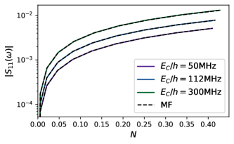
Figure 11: Numerical agreement between mean-field theory (black lines) and full-circuit time-evolution for different charging energies (i.e. different load impedances $Z_{0}$) against the average photon number in the gyrator.

Appendix D Circuit nonidealities

We start from the effective linear response theory proposed in Sect. B.5:

$$\bm{b_{\omega}}\simeq\bm{S}(\omega)\cdot\bm{a_{\omega}}=\left(\frac{\bm{Z}(\omega)}{Z_{\mathrm{TL}}}-1\right)^{-1}\cdot\left(\frac{\bm{Z}(\omega)}{Z_{\mathrm{TL}}}+1\right)\cdot\bm{a_{\omega}},$$ (143)

where

$$\bm{Z}(\omega)=i\omega\bm{L_{c}}+\left(i\omega\bm{C}+(i\omega\bm{L})^{-1}+iG\bm{\sigma_{y}}\right)^{-1}.$$ (144)

We now consider the general case $\bm{L_{c}}=L_{c}\bm{1}+dL_{c}\bm{\sigma_{z}}$, $\bm{C}=C_{0}\bm{1}+dC_{0}\bm{\sigma_{z}}-C_{12}\bm{\sigma_{x}}$ and $\bm{L}=L_{0}\bm{1}+dL_{0}\bm{\sigma_{z}}-L_{12}\bm{\sigma_{x}}$. Here $C_{12}$ and $L_{12}$ are the stray capacitive and inductive couplings respectively between the two internal gyrator modes. $dL_{c}$, $dC_{0}$ and $dL_{0}$ are due to asymmetries in the circuit. We highlight that $G$ is the average of the FENNEC interaction strength on both sides of the gyrator and is therefore insensitive to asymmetries – we only care about impedance matching with the characteristic impedance of the transmission lines.

We assume that $dL_{c}$, $dC_{0}$, $dL_{0}$, $C_{12}$ and $L_{12}$ are much smaller than $G$ and Taylor expand the perturbed impedance and scattering matrix $\bm{Z}^{\prime}(\omega)$ and $\bm{S}^{\prime}(\omega)$ to leading order in those quantities, i.e. $\bm{Z}^{\prime}(\omega)=\bm{Z}(\omega)+d\bm{Z}(\omega)$ and $\bm{S}^{\prime}(\omega)=\bm{S}(\omega)+d\bm{S}(\omega)$ where

$$d\bm{Z}(\omega)=i\omega dL_{c}\bm{\sigma_{z}}-\frac{i\omega dC_{0}-dL_{0}/(iL_{0}^{2}\omega)}{Z_{0}^{-2}(\omega)+G^{2}}\bm{\sigma_{z}}+\frac{i\omega C_{12}-L_{12}/(iL_{0}^{2}\omega)}{Z_{0}^{-2}(\omega)+G^{2}}\bm{\sigma_{x}},$$ (145)

and therefore

$$d\bm{S}(\omega)=-\left(\bm{1}-\bm{S}(\omega)\right)\cdot\frac{d\bm{Z}(\omega)}{2Z_{\mathrm{TL}}}\cdot\left(\bm{1}-\bm{S}(\omega)\right).$$ (146)

Recall that

$$\bm{S}(\omega)=\cos(2\theta_{\omega})\bm{1}+i\sin(2\theta_{\omega})\bm{\sigma_{y}},$$ (147)

and therefore we find that

$$\begin{split}d\bm{S}(\omega)=\frac{1-\cos(2\theta_{\omega})}{Z_{\mathrm{TL}}}\left(i\omega dL_{c}\bm{\sigma_{z}}-\frac{i\omega dC_{0}-dL_{0}/(iL_{0}^{2}\omega)}{Z_{0}^{-2}(\omega)+G^{2}}\bm{\sigma_{z}}+\frac{i\omega C_{12}-L_{12}/(iL_{0}^{2}\omega)}{Z_{0}^{-2}(\omega)+G^{2}}\bm{\sigma_{x}}\right).\end{split}$$ (148)

At central frequency $\omega_{0}=1/\sqrt{L_{0}C_{0}}$, where $Z_{0}^{-1}(\omega_{0})=0$, and at perfect impedance matching $\theta_{\omega}=\pi/4$ we observe that

$$\begin{split}d\bm{S}(\omega)=\frac{1}{Z_{\mathrm{TL}}}\left(i\omega dL_{c}\bm{\sigma_{z}}-\frac{i\omega_{0}dC_{0}-dL_{0}/(iL_{0}^{2}\omega_{0})}{G^{2}}\bm{\sigma_{z}}+\frac{i\omega_{0}C_{12}-L_{12}/(iL_{0}^{2}\omega_{0})}{G^{2}}\bm{\sigma_{x}}\right).\end{split}$$ (149)

Frequency mismatches, due to disorder in the circuit design, yield a $\bm{\sigma_{z}}$ error in $\bm{S}(\omega)$, which mostly affects reflection, whereas stray couplings result in a $\bm{\sigma_{x}}$ error, which instead mostly impacts transmission. We get the constraints

$$|\omega_{0}dL_{c}/Z_{\mathrm{TL}}|,\quad|\omega_{0}dC_{0}/Z_{\mathrm{TL}}G^{2}|,\quad|dL_{0}/(Z_{\mathrm{TL}}L_{0}^{2}\omega_{0}G^{2})|,\quad|\omega_{0}C_{12}/Z_{\mathrm{TL}}G^{2}|,\quad|L_{12}/(Z_{\mathrm{TL}}L_{0}^{2}\omega_{0}G^{2})|\ll 1.$$ (150)

These constraints come without surprise: Gyration is known to be fragile to circuit disorder and parasitic couplings. Another error specific to our circuit is due to deviations in the areas of the loops. This can in principle yield residual $\sin\hat{\varphi}_{k}$ potential terms. This is not captured by the calculation above. The leading order effect of this term is the renormalization of the photon number in the internal gyrator modes, or in another words, more compression and frequency mixing.

In Fig. 12 we plot the magnitude of circuit disorder resulting in a 1% error in the scattering matrix, found numerically using the least_squares algorithm in scipy. We indeed observe that larger $Z_{0}$ (i.e. $C_{0}\omega_{0}=1/Z_{0}$ and $L_{0}\omega_{0}=Z_{0}$) and smaller $L_{c}$ (i.e. larger $G$) yield larger tolerances. Similarly in Fig. 13 we observe that disorder in $L_{c}$ is not limited by $Z_{0}$ it is however impacted by $L_{c}$ itself– a smaller coupling inductance allows for stronger disorder.

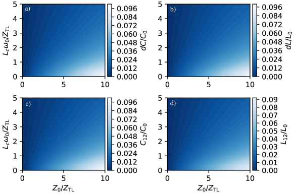
Figure 12: Magnitude of $dC$, $dL$, $dC_{12}$ and $dL_{12}$ resulting in a 1% error in the scattering matrix for a), b), c) and d) respectively.

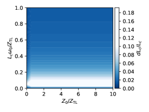
Figure 13: Magnitude of $dL_{c}$ resulting in a 1% error in the scattering matrix.

Appendix E Generic Lagrangian

We consider a generic circuit with total Lagrangian of the circuit is $\mathcal{L}=\mathcal{L}_{0}+\mathcal{L}_{\mathrm{c}p}$, where

$$\mathcal{L}_{0}=\dot{\bm{\Phi}}^{T}\cdot\frac{\bm{C_{0}}}{2}\cdot\dot{\bm{\Phi}}+\dot{\bm{\Phi}}^{T}\cdot\frac{\bm{C_{c}}}{2}\cdot\dot{\bm{\Phi}}+\left(\dot{\bm{\Phi}}-\bm{V_{J}}\right)^{T}\cdot\frac{\bm{C_{J}}}{2}\cdot\left(\dot{\bm{\Phi}}-\bm{V_{J}}\right)-U\left(\bm{\varphi}\right),$$ (151)

is the Lagrangian all the capacitive and inductive contributions commonly found in superconducting circuits and

$$\begin{split}\mathcal{L}_{\mathrm{i}nt}=-\varepsilon_{J,1}(\dot{\Phi}_{2},\varphi_{1})-\varepsilon_{J,2}(\dot{\Phi}_{1},\varphi_{2}),\quad\varepsilon_{J,k}(\dot{\Phi}_{\ell},\varphi_{k})=-\Delta_{k}\sqrt{1-T_{k}(V_{J,k},\dot{\Phi}_{\ell})\sin^{2}\left(\frac{\varphi_{k}-\varphi_{\mathrm{e}x,k}}{2}\right)},\end{split}$$ (152)

results from the FENNEC interaction alone. Here $\bm{\Phi}=\left(\Phi_{1},\ \Phi_{2}\right)$ is a vector comprising the branch flux $\Phi_{1}$ ($\Phi_{2}$) of the first (second) mode, $\bm{\varphi}=2\pi\bm{\Phi}/\Phi_{0}$ are the associated branch phases, $\bm{C_{0}}$ and $\bm{C_{c}}$ are capacitance matrices due to the shunt capacitors and the coupling capacitors respectively, $\bm{C_{J}}$ is the capacitance matrix associated with the coupling to the control voltage lines $\bm{V_{J}}$, $U(\bm{\varphi})$ is the potential energy of the two modes defined by the shaded regions in the circuit, $\Delta_{1}$ ($\Delta_{2}$) is the ABS energy of the small junction of mode 1 (mode 2), $T_{1}$ ($T_{2}$) is the transmission probability of the small junction of mode 1 (mode 2), $\Phi_{\mathrm{e}x,1}$ ($\Phi_{\mathrm{e}x,2}$) is an external flux threading the loop enclosing the small junction and the shaded region of mode 1 (mode 2).

E.1 Taylor-expanded form

We will now simplify the interaction Lagrangian. First we do a Taylor expansion in $\dot{\Phi}_{k}$,

$$\begin{split}\mathcal{L}_{\mathrm{i}nt}=-\sum_{n=0}^{\infty}\frac{\dot{\Phi}_{2}^{n}}{n!}\frac{\partial^{n}\varepsilon_{J,1}(\dot{\Phi}_{2},\varphi_{1})}{\partial\dot{\Phi}_{2}^{n}}\Big{|}_{\dot{\Phi}_{2}=0}-\sum_{n=0}^{\infty}\frac{\dot{\Phi}_{1}^{n}}{n!}\frac{\partial^{n}\varepsilon_{J,2}(\dot{\Phi}_{1},\varphi_{2})}{\partial\dot{\Phi}_{1}^{n}}\Big{|}_{\dot{\Phi}_{1}=0}\end{split}$$ (153)

Second we also do a Taylor expansion in $T_{k}$,

$$\begin{split}\mathcal{L}_{\mathrm{i}nt}=\sum_{n,m=0}^{\infty}g_{1,n,m}\frac{\dot{\Phi}_{2}^{n}}{n!}\sin^{2m}\left(\frac{\varphi_{1}-\varphi_{\mathrm{e}x,1}}{2}\right)+\sum_{n,m=0}^{\infty}g_{2,n,m}\frac{\dot{\Phi}_{1}^{n}}{n!}\sin^{2m}\left(\frac{\varphi_{2}-\varphi_{\mathrm{e}x,2}}{2}\right),\end{split}$$ (154)

where we defined the couplings

$$g_{1,n,m}=(-1)^{m}\begin{pmatrix}1/2\\ m\end{pmatrix}\Delta_{1}\left(\frac{\partial^{n}T_{1}^{m}(V_{J,1},\dot{\Phi}_{2})}{\partial\dot{\Phi}_{2}^{n}}\Big{|}_{\dot{\Phi}_{2}=0}\right),\quad g_{2,n,m}=(-1)^{m}\begin{pmatrix}1/2\\ m\end{pmatrix}\Delta_{2}\left(\frac{\partial^{n}T_{2}^{m}(V_{J,2},\dot{\Phi}_{1})}{\partial\dot{\Phi}_{1}^{n}}\Big{|}_{\dot{\Phi}_{1}=0}\right).$$ (155)

In vectorized form the Lagrangian then takes the form

$$\mathcal{L}=\dot{\bm{\Phi}}^{T}\cdot\frac{\bm{C}(\bm{\varphi})}{2}\cdot\dot{\bm{\Phi}}+\left[\frac{\bm{q_{0}}^{T}(\bm{\varphi})}{2}\cdot\dot{\bm{\Phi}}+\dot{\bm{\Phi}}^{T}\cdot\frac{\bm{q_{0}}(\bm{\varphi})}{2}\right]+\sum_{n=3}^{\infty}\left[\bm{1_{1\times 2}}\cdot\frac{\bm{g_{n}}(\bm{\varphi})}{2}\cdot\frac{\dot{\bm{\Phi}}^{\circ n}}{n!}+\frac{\dot{\bm{\Phi}}^{T\circ n}}{n!}\cdot\frac{\bm{g_{n}}(\bm{\varphi})}{2}\cdot\bm{1_{2\times 1}}\right]-U\left(\bm{\varphi}\right),$$ (156)

where we defined the charge offset

$$\bm{q_{0}}(\bm{\varphi})=-\bm{C_{J}}\cdot\bm{V_{J}}+\bm{g_{1}}(\bm{\varphi})\cdot\bm{1_{2\times 1}},$$ (157)

the total capacitance matrix

$$\bm{C}(\bm{\varphi})=\bm{C_{0}}+\bm{C_{c}}+\bm{C_{J}}+\bm{g_{2}}(\bm{\varphi}),$$ (158)

the diagonal matrices

$$\bm{g_{n}}(\bm{\varphi})=\sum_{m=0}^{\infty}\mathrm{diag}\left(g_{2,n,m}\sin^{2m}\left(\dfrac{\varphi_{2}-\varphi_{\mathrm{e}x,2}}{2}\right),g_{1,n,m}\sin^{2m}\left(\dfrac{\varphi_{1}-\varphi_{\mathrm{e}x,1}}{2}\right)\right),$$ (159)

and where $\circ$ is the Hadamard product. We highlight the identity

$$\sin^{2m}(x/2)=-\frac{(-1)^{m}}{4^{m}}\left(2\sum_{k=0}^{m-1}(-1)^{k}\begin{pmatrix}2m\\ k\end{pmatrix}\cos((m-k)x)-(-1)^{m}\begin{pmatrix}2m\\ m\end{pmatrix}\right)$$ (160)

obtained with the help of the binomial theorem.

E.2 Canonical quantization

In virtue of Hamilton’s principle, the canonical charges, $\bm{q}$, associated with  $\bm{\Phi}$ are given by

$$\begin{split}\bm{q}=\frac{\partial\mathcal{L}}{\partial\dot{\bm{\Phi}}}=\bm{q_{0}}(\bm{\varphi})+\bm{C}(\bm{\varphi})\cdot\dot{\bm{\Phi}}+\sum_{n=2}^{\infty}\bm{g_{n+1}}(\bm{\varphi})\cdot\frac{\dot{\bm{\Phi}}^{\circ n}}{n!},\end{split}$$ (161)

where we observe that $\bm{q}$ is nonlinear in $\dot{\bm{\Phi}}$.

Let’s consider $\bm{g_{n+1}}\to\lambda\bm{g_{n+1}}$ to be a perturbation for $n\geq 2$. We will now write $\dot{\bm{\Phi}}$ using a perturbative expansion,

$$\dot{\bm{\Phi}}=\bm{C}^{-1}(\bm{\varphi})\cdot\left(\bm{q}-\bm{q_{0}}(\bm{\varphi})\right)+\sum_{k=1}^{\infty}\lambda^{k}\bm{X_{k}}(\bm{q})=\sum_{k=0}^{\infty}\lambda^{k}\bm{X_{k}}(\bm{q}),\quad\bm{X_{0}}(\bm{q})=\bm{C}^{-1}(\bm{\varphi})\cdot\left(\bm{q}-\bm{q_{0}}(\bm{\varphi})\right),$$ (162)

where $\lambda$ is used to define the order of the expansion. Plugging this expansion in the definition of the canonical charges yields

$$\begin{split}0=\sum_{k=1}^{\infty}\lambda^{k-1}\bm{C}(\bm{\varphi})\cdot\bm{X_{k}}+\sum_{n=2}^{\infty}\bm{g_{n+1}}(\bm{\varphi})\cdot\frac{1}{n!}\left(\sum_{k=0}^{\infty}\lambda^{k}\bm{X_{k}}\right)^{\circ n}\end{split}$$ (163)

where we can then use the binomial theorem to obtain

$$\begin{split}\frac{1}{n!}\left(\sum_{k=0}^{\infty}\lambda^{k}\bm{X_{k}}\right)^{\circ n}=\lim_{K\to\infty}\sum_{m_{0},m_{1},\cdots,m_{K}=0}^{n}\delta_{n,\sum_{j=0}^{K}m_{j}}\frac{\left(\lambda^{0}\bm{X_{0}}\right)^{\circ m_{0}}}{m_{0}!}\circ\frac{\left(\lambda^{1}\bm{X_{1}}\right)^{\circ m_{1}}}{m_{1}!}\circ\cdots\circ\frac{\left(\lambda^{K}\bm{X_{K}}\right)^{\circ m_{K}}}{m_{K}!},\end{split}$$ (164)

where $\delta_{ij}=\begin{cases}1,&i=j\\ 0,&i\neq j\end{cases}$ is the discrete Dirac delta function. By grouping terms of same order in $\lambda$ we find that

$$\begin{split}\bm{X_{k}}=-\sum_{n=2}^{\infty}\bm{C}^{-1}(\bm{\varphi})\cdot\bm{g_{n+1}}(\bm{\varphi})\cdot\sum_{m_{1}=0}^{(k-1)/1}\cdots\sum_{m_{k-1}=0}^{(k-1)/(k-1)}\delta_{k-1,\sum_{j=1}^{k-1}jm_{j}}\frac{\left(\lambda^{0}\bm{X_{0}}\right)^{\circ\left(n-\sum_{j=1}^{k-1}m_{j}\right)}}{\left(n-\sum_{j=1}^{k-1}m_{j}\right)!}\circ\frac{\left(\lambda^{1}\bm{X_{1}}\right)^{\circ m_{1}}}{m_{1}!}\\ \circ\cdots\circ\frac{\left(\lambda^{k-1}\bm{X_{k-1}}\right)^{\circ m_{k-1}}}{m_{k-1}!}.\end{split}$$ (165)

The first correction terms are explicitly

$$\bm{X_{0}}=\bm{C}^{-1}(\bm{\varphi})\cdot\left(\bm{q}-\bm{q_{0}}(\bm{\varphi})\right),$$ (166)

$$\bm{X_{1}}=-\sum_{n=2}^{\infty}\bm{C}^{-1}(\bm{\varphi})\cdot\bm{g_{n+1}}(\bm{\varphi})\cdot\frac{\bm{X_{0}}^{\circ n}}{n!},$$ (167)

$$\bm{X_{2}}=-\sum_{n=2}^{\infty}\bm{C}^{-1}(\bm{\varphi})\cdot\bm{g_{n+1}}(\bm{\varphi})\cdot\frac{\bm{X_{0}}^{\circ(n-1)}}{(n-1)!}\circ\bm{X_{1}}$$ (168)

$$\bm{X_{3}}=-\sum_{n=2}^{\infty}\bm{C}^{-1}(\bm{\varphi})\cdot\bm{g_{n+1}}(\bm{\varphi})\cdot\left(\frac{\bm{X_{0}}^{\circ(n-1)}}{(n-1)!}\circ\bm{X_{2}}+\frac{\bm{X_{0}}^{\circ(n-2)}}{(n-2)!}\circ\frac{\bm{X_{1}}^{\circ 2}}{2!}\right)$$ (169)

$$\cdots$$ (170)

We emphasize that $\left[\bm{\Phi},\bm{q}\right]=i$ following the canonical quantization.

E.3 Full system Hamiltonian

Now that we have expressions for the canonical charges we can write the Hamiltonian. The total system Hamiltonian, given by $\mathcal{H}=\dot{\bm{\Phi}}^{T}\cdot\bm{q}-\mathcal{L}$, is (for $\lambda=1$)

$$\mathcal{H}=\dot{\bm{\Phi}}^{T}\cdot\frac{\bm{C}(\bm{\varphi})}{2}\cdot\dot{\bm{\Phi}}+\sum_{n=3}^{\infty}\left[\bm{1_{1\times 2}}\cdot\frac{(n-1)\bm{g_{n}}(\bm{\varphi})}{2}\cdot\frac{\dot{\bm{\Phi}}^{\circ n}}{n!}+\frac{\dot{\bm{\Phi}}^{T\circ n}}{n!}\cdot\frac{(n-1)\bm{g_{n}}(\bm{\varphi})}{2}\cdot\bm{1_{2\times 1}}\right]+U\left(\bm{\varphi}\right),\quad\dot{\bm{\Phi}}=\sum_{k=0}^{\infty}\bm{X_{k}}(\bm{q}).$$ (171)

We can also divide the system Hamiltonian $\mathcal{H}=\mathcal{H}_{\mathrm{quad}}+\mathcal{H}_{\mathrm{nln}}$ into two parts:

$$\mathcal{H}_{\mathrm{quad}}=\left(\bm{q}-\bm{q_{0}}(\bm{\varphi})\right)^{T}\cdot\frac{\bm{C}^{-1}(\bm{\varphi})}{2}\cdot\left(\bm{q}-\bm{q_{0}}(\bm{\varphi})\right)+U\left(\bm{\varphi}\right)$$ (172)

involves all the contributions up to quadratic order in the charge operators $\bm{q}-\bm{q_{0}}$, and

$$\begin{split}\mathcal{H}_{\mathrm{nln}}&=\left(\sum_{k=0}^{\infty}\bm{X_{k}}(\bm{q})\right)^{T}\cdot\frac{\bm{C}(\bm{\varphi})}{2}\cdot\left(\sum_{k=0}^{\infty}\bm{X_{k}}(\bm{q})\right)-\bm{X_{0}}^{T}\cdot\frac{\bm{C}(\bm{\varphi})}{2}\cdot\bm{X_{0}}\\ &+\sum_{n=3}^{\infty}\left[\bm{1_{1\times 2}}\cdot\frac{(n-1)\bm{g_{n}}(\bm{\varphi})}{2}\cdot\frac{\left(\sum_{k=0}^{\infty}\bm{X_{k}}(\bm{q})\right)^{\circ n}}{n!}+\frac{\left(\sum_{k=0}^{\infty}\bm{X_{k}}(\bm{q})\right)^{T\circ n}}{n!}\cdot\frac{(n-1)\bm{g_{n}}(\bm{\varphi})}{2}\cdot\bm{1_{2\times 1}}\right]\end{split}$$ (173)

comprises all remaining terms that are nonlinear in the charge operators, due to higher derivatives of the transmission coefficients.

$q$-quadratic Hamiltonian in expanded form

Let us consider $g_{j,1,1}$ to be the largest components by design and any other $g_{j,n,m}\to\lambda g_{j,n,m}$ be an error term. Moreover we consider the coupling capacitance $C_{c}\to\lambda C_{c}$ to be an error on the same order. We want to write the q-quadratic Hamiltonian to leading order in $\lambda$. The capacitance matrix to have the form

$$\bm{C}(\bm{\varphi})=\begin{pmatrix}C_{1}+\sum_{\ell=1}^{\infty}\lambda\Lambda_{1,2,\ell}\cos(\ell(\varphi_{2}-\varphi_{\mathrm{e}x,2}))&-\lambda C_{c}\\ -\lambda C_{c}&C_{2}+\sum_{\ell=1}^{\infty}\lambda\Lambda_{2,2,\ell}\cos(\ell(\varphi_{1}-\varphi_{\mathrm{e}x,1}))\end{pmatrix},$$ (174)

where $C_{j}$ are the total capacitances and where we defined the coefficients

$$\Lambda_{1,n,\ell}=-\sum_{m=1}^{\infty}\sum_{k=0}^{m-1}\dfrac{2(-1)^{m+k}g_{2,n,m}}{4^{m}}\begin{pmatrix}2m\\ k\end{pmatrix}\delta_{m-k,\ell},\quad\Lambda_{2,n,\ell}=-\sum_{m=1}^{\infty}\sum_{k=0}^{m-1}\dfrac{2(-1)^{m+k}g_{1,n,m}}{4^{m}}\begin{pmatrix}2m\\ k\end{pmatrix}\delta_{m-k,\ell}.$$ (175)

To leading order in $\lambda$ we find that

$$\bm{C}^{-1}(\bm{\varphi})\approx\begin{pmatrix}\left(1-\sum_{\ell=1}^{\infty}\lambda\Lambda_{1,2,\ell}C_{1}^{-1}\cos(\ell(\varphi_{2}-\varphi_{\mathrm{e}x,2}))\right)C_{1}^{-1}&\lambda C_{c}C_{1}^{-1}C_{2}^{-1}\\ \lambda C_{c}C_{1}^{-1}C_{2}^{-1}&\left(1-\sum_{\ell=1}^{\infty}\lambda\Lambda_{2,2,\ell}C_{2}^{-1}\cos(\ell(\varphi_{1}-\varphi_{\mathrm{e}x,1}))\right)C_{2}^{-1}\end{pmatrix}.$$ (176)

The charge offsets can be written as

$$\bm{q_{0}}(\bm{\varphi})=\begin{pmatrix}q_{01}-g_{1}\cos\left(\varphi_{2}-\varphi_{\mathrm{e}x,2}\right)+\sum_{\ell=2}^{\infty}\lambda\Lambda_{1,1,\ell}\cos(\ell(\varphi_{2}-\varphi_{\mathrm{e}x,2}))\\ q_{02}-g_{2}\cos\left(\varphi_{1}-\varphi_{\mathrm{e}x,1}\right)+\sum_{\ell=2}^{\infty}\lambda\Lambda_{2,1,\ell}\cos(\ell(\varphi_{1}-\varphi_{\mathrm{e}x,1})),\end{pmatrix},$$ (177)

where $q_{0j}$ are some scalars and where we defined the couplings

$$g_{1}=-g_{2,1,1}/2,\quad g_{2}=-g_{1,1,1}/2.$$ (178)

The $q$-quadratic Hamiltonian to leading order in $\lambda$ then approximately takes the form

$$\begin{split}\mathcal{H}_{\mathrm{quad}}=\frac{\left(q_{1}-q_{01}+g_{1}\cos\left(\varphi_{2}-\varphi_{\mathrm{e}x,2}\right)\right)^{2}}{2C_{1}}+\frac{\left(q_{2}-q_{02}+g_{2}\cos\left(\varphi_{1}-\varphi_{\mathrm{e}x,1}\right)\right)^{2}}{2C_{2}}+U\left(\varphi_{1},\varphi_{2}\right)+\lambda\mathcal{H}_{\mathrm{quad}}^{\lambda}+\mathcal{O}(\lambda^{2}),\end{split}$$ (179)

and the error Hamiltonian

$$\begin{split}\mathcal{H}_{\mathrm{quad}}^{\lambda}=&-\frac{\left(q_{1}-q_{01}\right)}{C_{1}}\sum_{\ell=2}^{\infty}\Lambda_{1,1,\ell}\cos(\ell(\varphi_{2}-\varphi_{\mathrm{e}x,2}))-\frac{\left(q_{2}-q_{02}\right)}{C_{2}}\sum_{\ell=2}^{\infty}\Lambda_{2,1,\ell}\cos(\ell(\varphi_{1}-\varphi_{\mathrm{e}x,1}))\\ &-\frac{\left(q_{1}-q_{01}\right)^{2}}{2C_{1}^{2}}\sum_{\ell=1}^{\infty}\Lambda_{1,2,\ell}\cos(\ell(\varphi_{2}-\varphi_{\mathrm{e}x,2}))-\frac{\left(q_{2}-q_{02}\right)^{2}}{2C_{2}^{2}}\sum_{\ell=1}^{\infty}\Lambda_{2,2,\ell}\cos(\ell(\varphi_{1}-\varphi_{\mathrm{e}x,1}))\\ &+\frac{C_{c}}{C_{1}C_{2}}\left(q_{1}-q_{01}\right)\left(q_{2}-q_{02}\right).\end{split}$$ (180)

q-nonlinear Hamiltonian in expanded form

To leading order in $\bm{g_{n}}$ for $n\geq 3$ we can approximate

$$\mathcal{H}_{\mathrm{nln}}\approx-\sum_{n=3}^{\infty}\left[\bm{1_{1\times 2}}\cdot\frac{\lambda\bm{g_{n}}(\bm{\varphi})}{2}\cdot\frac{\left(\bm{C}^{-1}(\bm{\varphi})\cdot\left(\bm{q}-\bm{q_{0}}(\bm{\varphi})\right)\right)^{\circ n}}{n!}+\frac{\left(\bm{C}^{-1}(\bm{\varphi})\cdot\left(\bm{q}-\bm{q_{0}}(\bm{\varphi})\right)\right)^{T\circ n}}{n!}\cdot\frac{\lambda\bm{g_{n}}(\bm{\varphi})}{2}\cdot\bm{1_{2\times 1}}\right].$$ (181)

To leading order in $\lambda$ we find that $\mathcal{H}_{\mathrm{nln}}\approx\lambda\mathcal{H}_{\mathrm{nln}}^{\lambda}+\mathcal{O}\left(\lambda^{2}\right)$ with

$$\begin{split}\mathcal{H}_{\mathrm{nln}}^{\lambda}=-\sum_{n=3}^{\infty}\frac{\left(q_{1}-q_{01}\right)^{n}}{n!C_{1}^{n}}\sum_{\ell=1}^{\infty}\Lambda_{1,n,\ell}\cos(\ell(\varphi_{2}-\varphi_{\mathrm{e}x,2}))-\sum_{n=3}^{\infty}\frac{\left(q_{2}-q_{02}\right)^{n}}{n!C_{2}^{n}}\sum_{\ell=1}^{\infty}\Lambda_{2,n,\ell}\cos(\ell(\varphi_{1}-\varphi_{\mathrm{e}x,1}))\\ -\sum_{n=3}^{\infty}\frac{\left(q_{1}-q_{01}\right)^{n}}{n!C_{1}^{n}}\xi_{1,n}-\sum_{n=3}^{\infty}\frac{\left(q_{2}-q_{02}\right)^{n}}{n!C_{2}^{n}}\xi_{2,n},\end{split}$$ (182)

where we defined the coefficients

$$\xi_{1,n}=\sum_{m=0}^{\infty}\dfrac{g_{2,n,m}}{4^{m}}\begin{pmatrix}2m\\ m\end{pmatrix},\quad\xi_{2,n}=\sum_{m=0}^{\infty}\dfrac{g_{1,n,m}}{4^{m}}\begin{pmatrix}2m\\ m\end{pmatrix}.$$ (183)

Approximate form

Combining the results of the previous sections with $\lambda=1$ we therefore find the approximate Hamiltonian

$$\begin{split}\mathcal{H}\simeq\frac{\left(q_{1}-q_{01}+g_{1}\cos\left(\varphi_{2}-\varphi_{\mathrm{e}x,2}\right)\right)^{2}}{2C_{1}}+\frac{\left(q_{2}-q_{02}+g_{2}\cos\left(\varphi_{1}-\varphi_{\mathrm{e}x,1}\right)\right)^{2}}{2C_{2}}+U\left(\varphi_{1},\varphi_{2}\right)+\mathcal{H}_{\mathrm{err}},\end{split}$$ (184)

where we defined the error Hamiltonian

$$\begin{split}\mathcal{H}_{\mathrm{err}}=&-\frac{\left(q_{1}-q_{01}\right)}{C_{1}}\sum_{\ell=2}^{\infty}\Lambda_{1,1,\ell}\cos(\ell(\varphi_{2}-\varphi_{\mathrm{e}x,2}))-\frac{\left(q_{2}-q_{02}\right)}{C_{2}}\sum_{\ell=2}^{\infty}\Lambda_{2,1,\ell}\cos(\ell(\varphi_{1}-\varphi_{\mathrm{e}x,1}))\\ &-\sum_{n=2}^{\infty}\frac{\left(q_{1}-q_{01}\right)^{n}}{n!C_{1}^{n}}\sum_{\ell=1}^{\infty}\Lambda_{1,n,\ell}\cos(\ell(\varphi_{2}-\varphi_{\mathrm{e}x,2}))-\sum_{n=2}^{\infty}\frac{\left(q_{2}-q_{02}\right)^{n}}{n!C_{2}^{n}}\sum_{\ell=1}^{\infty}\Lambda_{2,n,\ell}\cos(\ell(\varphi_{1}-\varphi_{\mathrm{e}x,1}))\\ &-\sum_{n=3}^{\infty}\frac{\left(q_{1}-q_{01}\right)^{n}}{n!C_{1}^{n}}\xi_{1,n}-\sum_{n=3}^{\infty}\frac{\left(q_{2}-q_{02}\right)^{n}}{n!C_{2}^{n}}\xi_{2,n}+\frac{C_{c}}{C_{1}C_{2}}\left(q_{1}-q_{01}\right)\left(q_{2}-q_{02}\right).\end{split}$$ (185)

Here the couplings are explicitly

$$g_{1}=\frac{\Delta_{2}}{4}\left(\frac{\partial T_{2}(V_{J,2},\dot{\Phi}_{1})}{\partial\dot{\Phi}_{1}}\Big{|}_{\dot{\Phi}_{1}=0}\right),$$ (186)

$$g_{2}=\frac{\Delta_{1}}{4}\left(\frac{\partial T_{1}(V_{J,1},\dot{\Phi}_{2})}{\partial\dot{\Phi}_{2}}\Big{|}_{\dot{\Phi}_{2}=0}\right),$$ (187)

$$\Lambda_{1,n,\ell}=-\sum_{m=1}^{\infty}\sum_{k=0}^{m-1}\dfrac{2(-1)^{k}}{4^{m-1}}\begin{pmatrix}1/2\\ m\end{pmatrix}\begin{pmatrix}2m\\ k\end{pmatrix}\delta_{m-k,\ell}\frac{\Delta_{2}}{4}\left(\frac{\partial^{n}T_{2}^{m}(V_{J,2},\dot{\Phi}_{1})}{\partial\dot{\Phi}_{1}^{n}}\Big{|}_{\dot{\Phi}_{1}=0}\right),$$ (188)

$$\Lambda_{2,n,\ell}=-\sum_{m=1}^{\infty}\sum_{k=0}^{m-1}\dfrac{2(-1)^{k}}{4^{m-1}}\begin{pmatrix}1/2\\ m\end{pmatrix}\begin{pmatrix}2m\\ k\end{pmatrix}\delta_{m-k,\ell}\frac{\Delta_{1}}{4}\left(\frac{\partial^{n}T_{1}^{m}(V_{J,1},\dot{\Phi}_{2})}{\partial\dot{\Phi}_{2}^{n}}\Big{|}_{\dot{\Phi}_{2}=0}\right),$$ (189)

$$\xi_{1,n}=\sum_{m=0}^{\infty}\dfrac{(-1)^{m}}{4^{m-1}}\begin{pmatrix}1/2\\ m\end{pmatrix}\begin{pmatrix}2m\\ m\end{pmatrix}\frac{\Delta_{2}}{4}\left(\frac{\partial^{n}T_{2}^{m}(V_{J,2},\dot{\Phi}_{1})}{\partial\dot{\Phi}_{1}^{n}}\Big{|}_{\dot{\Phi}_{1}=0}\right),$$ (190)

$$\xi_{2,n}=\sum_{m=0}^{\infty}\dfrac{(-1)^{m}}{4^{m-1}}\begin{pmatrix}1/2\\ m\end{pmatrix}\begin{pmatrix}2m\\ m\end{pmatrix}\frac{\Delta_{1}}{4}\left(\frac{\partial^{n}T_{1}^{m}(V_{J,1},\dot{\Phi}_{2})}{\partial\dot{\Phi}_{2}^{n}}\Big{|}_{\dot{\Phi}_{2}=0}\right).$$ (191)

Tolerance values of the higher derivatives in the error terms are ultimately determined by the mode impedances, i.e.

$$\left|\sum_{m=1}^{\infty}\sum_{k=0}^{m-1}\dfrac{2(-1)^{k}}{4^{m-1}}\begin{pmatrix}1/2\\ m\end{pmatrix}\begin{pmatrix}2m\\ k\end{pmatrix}\delta_{m-k,\ell}\frac{(2e)^{n}\Delta_{2}}{4n!C_{1}^{n}}\left(\frac{\partial^{n}T_{2}^{m}(V_{J,2},\dot{\Phi}_{1})}{\partial\dot{\Phi}_{1}^{n}}\Big{|}_{\dot{\Phi}_{1}=0}\right)\right|\ll\sqrt{\frac{4\pi Z_{1}}{R_{Q}}}^{n},$$ (192)

$$\left|\sum_{m=1}^{\infty}\sum_{k=0}^{m-1}\dfrac{2(-1)^{k}}{4^{m-1}}\begin{pmatrix}1/2\\ m\end{pmatrix}\begin{pmatrix}2m\\ k\end{pmatrix}\delta_{m-k,\ell}\frac{(2e)^{n}\Delta_{1}}{4n!C_{2}^{n}}\left(\frac{\partial^{n}T_{1}^{m}(V_{J,1},\dot{\Phi}_{2})}{\partial\dot{\Phi}_{2}^{n}}\Big{|}_{\dot{\Phi}_{2}=0}\right)\right|\ll\sqrt{\frac{4\pi Z_{2}}{R_{Q}}}^{n},$$ (193)

where $Z_{j}$ is the impedance of mode $j$ and $R_{Q}\simeq 6.5\leavevmode\nobreak\$k$\Omega$ is the resistance quantum. The constraints are obtained by considering the smallest non-zero matrix elements of the charge quadrature $q_{j}$ to be given by $i2e\sqrt{R_{Q}/(4\pi Z_{j})}$.

Appendix F Classical scattering matrix for a 3-port circulator

Following standard circuit theory Carlin and Giordano (1964), we can compute the classical (linear) scattering matrix response for a gyrator-based 3-port circulator with symmetric LC-resonator loads at their ports, see Fig. Fig. 4b). Such matrix relates the amplitudes of single-tone input ($a_{n}(\omega)=(V_{n}+Z_{\mathrm{TL}}I_{n})/\sqrt{Z_{\mathrm{TL}}}$) and output ($b_{n}(\omega)=(V_{n}-Z_{\mathrm{TL}}I_{n})/\sqrt{Z_{\mathrm{TL}}}$) signals, where $I_{n}$ ($V_{n}$) is the current (voltage) of port $n$, such that $\bm{b}=\bm{S}(\omega)\bm{a}$. Solving Kirchhoff’s equations in the frequency domain, we obtain

$$\bm{S}= \frac{1}{r}\left(\begin{array}[]{ccc}R^{2}(Z_{\mathrm{TL}}-\tilde{Z}_{0})^{2}-Z_{\mathrm{TL}}^{2}\tilde{Z}_{0}^{2}&2R\tilde{Z}_{0}(\tilde{Z}_{0}(R+Z_{\mathrm{TL}})-RZ_{\mathrm{TL}})&2R\tilde{Z}_{0}(R(Z_{\mathrm{TL}}+\tilde{Z}_{0})-Z_{\mathrm{TL}}\tilde{Z}_{0})\\ 2R\tilde{Z}_{0}(R(\tilde{Z}_{0}-Z_{\mathrm{TL}})-Z_{\mathrm{TL}}\tilde{Z}_{0})&R^{2}(Z_{\mathrm{TL}}-\tilde{Z}_{0})^{2}-Z_{\mathrm{TL}}^{2}\tilde{Z}_{0}^{2}&-2R\tilde{Z}_{0}(R(Z_{\mathrm{TL}}+\tilde{Z}_{0})+Z_{\mathrm{TL}}\tilde{Z}_{0})\\ 2R\tilde{Z}_{0}(R(Z_{\mathrm{TL}}+\tilde{Z}_{0})+Z_{\mathrm{TL}}\tilde{Z}_{0})&-2R\tilde{Z}_{0}(R(Z_{\mathrm{TL}}+\tilde{Z}_{0})-Z_{\mathrm{TL}}\tilde{Z}_{0})&R^{2}(Z_{\mathrm{TL}}+\tilde{Z}_{0})^{2}-Z_{\mathrm{TL}}^{2}\tilde{Z}_{0}^{2}\\ \end{array}\right).$$ (197)

Here, we have defined the parameters

$$r= (Z_{\mathrm{TL}}^{2}\tilde{Z}_{0}^{2}-R^{2}(Z_{\mathrm{TL}}-3\tilde{Z}_{0})(Z_{\mathrm{TL}}+\tilde{Z}_{0})),\qquad\tilde{Z}_{0}(\omega)=Z_{0}\frac{-i\omega\omega_{r}}{\omega^{2}-\omega_{r}^{2}},$$ (198)

and $Z_{0}=\sqrt{L_{0}/C_{0}}$ and $\omega_{0}=1/\sqrt{L_{0}C_{0}}$. Impedance-matching the whole system to the reference transmission-lines ($R=Z_{0}=Z_{\mathrm{TL}}$), and working on resonance condition ($\omega=\omega_{r}$), the linear response becomes that ideal circulator

$$\bm{S}\rightarrow\begin{pmatrix}0&1&0\\ 0&0&-1\\ 1&0&0\end{pmatrix}.$$ (199)

References

- Naaman and Aumentado (2022) Ofer Naaman and José Aumentado, “Synthesis of parametrically coupled networks,” PRX Quantum 3, 020201 (2022).
- Ranzani and Aumentado (2014) Leonardo Ranzani and José Aumentado, “A geometric description of nonreciprocity in coupled two-mode systems,” 16, 103027 (2014).
- Ranzani and Aumentado (2015) Leonardo Ranzani and José Aumentado, “Graph-based analysis of nonreciprocity in coupled-mode systems,” 17, 023024 (2015).
- Kamal et al. (2011) Archana Kamal, John Clarke, and M. H. Devoret, “Noiseless non-reciprocity in a parametric active device,” Nature Physics 7, 311–315 (2011).
- Kerckhoff et al. (2015) Joseph Kerckhoff, Kevin Lalumière, Benjamin J. Chapman, Alexandre Blais, and K. W. Lehnert, “On-chip superconducting microwave circulator from synthetic rotation,” Phys. Rev. Applied 4, 034002 (2015).
- Sliwa et al. (2015) K. M. Sliwa, M. Hatridge, A. Narla, S. Shankar, L. Frunzio, R. J. Schoelkopf, and M. H. Devoret, “Reconfigurable josephson circulator/directional amplifier,” Phys. Rev. X 5, 041020 (2015).
- Koch et al. (2010) Jens Koch, Andrew A. Houck, Karyn Le Hur, and S. M. Girvin, “Time-reversal-symmetry breaking in circuit-qed-based photon lattices,” Phys. Rev. A 82, 043811 (2010).
- Chapman et al. (2019) Benjamin J. Chapman, Eric I. Rosenthal, and K. W. Lehnert, “Design of an on-chip superconducting microwave circulator with octave bandwidth,” Phys. Rev. Applied 11, 044048 (2019).
- Dinc et al. (2017) Tolga Dinc, Mykhailo Tymchenko, Aravind Nagulu, Dimitrios Sounas, Andrea Alu, and Harish Krishnaswamy, “Synchronized conductivity modulation to realize broadband lossless magnetic-free non-reciprocity,” Nature Communications 8, 795 (2017).
- Müller et al. (2018) Clemens Müller, Shengwei Guan, Nicolas Vogt, Jared H. Cole, and Thomas M. Stace, “Passive on-chip superconducting circulator using a ring of tunnel junctions,” Phys. Rev. Lett. 120, 213602 (2018).
- Richman and Taylor (2021) Brittany Richman and Jacob M. Taylor, “Circulation by microwave-induced vortex transport for signal isolation,” PRX Quantum 2, 030309 (2021).
- Navarathna et al. (2022) Rohit Navarathna, Dat Thanh Le, Andrés Rosario Hamann, Hien Duy Nguyen, Thomas M. Stace, and Arkady Fedorov, “Passive superconducting circulator on a chip,” (2022).
- Abdo et al. (2017) Baleegh Abdo, Markus Brink, and Jerry M. Chow, “Gyrator operation using josephson mixers,” Phys. Rev. Applied 8, 034009 (2017).
- Malz et al. (2018) Daniel Malz, László D. Tóth, Nathan R. Bernier, Alexey K. Feofanov, Tobias J. Kippenberg, and Andreas Nunnenkamp, “Quantum-limited directional amplifiers with optomechanics,” Phys. Rev. Lett. 120, 023601 (2018).
- Thorbeck et al. (2017) T. Thorbeck, S. Zhu, E. Leonard, R. Barends, J. Kelly, John M. Martinis, and R. McDermott, “Reverse isolation and backaction of the slug microwave amplifier,” Phys. Rev. Applied 8, 054007 (2017).
- Abdo et al. (2014) Baleegh Abdo, Katrina Sliwa, S. Shankar, Michael Hatridge, Luigi Frunzio, Robert Schoelkopf, and Michel Devoret, “Josephson directional amplifier for quantum measurement of superconducting circuits,” Phys. Rev. Lett. 112, 167701 (2014).
- Metelmann and Clerk (2015) A. Metelmann and A. A. Clerk, “Nonreciprocal photon transmission and amplification via reservoir engineering,” Phys. Rev. X 5, 021025 (2015).
- Abdo et al. (2013) Baleegh Abdo, Katrina Sliwa, Luigi Frunzio, and Michel Devoret, “Directional amplification with a josephson circuit,” Phys. Rev. X 3, 031001 (2013).
- C. et al. (2015) Macklin C., O’Brien K., Hover D., Schwartz M. E., Bolkhovsky V., Zhang X., Oliver W. D., and Siddiqi I., “A near–quantum-limited josephson traveling-wave parametric amplifier,” Science 350, 307–310 (2015).
- Ho Eom et al. (2012) Byeong Ho Eom, Peter K. Day, Henry G. LeDuc, and Jonas Zmuidzinas, “A wideband, low-noise superconducting amplifier with high dynamic range,” Nature Physics 8, 623–627 (2012).
- Vissers et al. (2016) M. R. Vissers, R. P. Erickson, H. S. Ku, Leila Vale, Xian Wu, G. C. Hilton, and D. P. Pappas, “Low-noise kinetic inductance traveling-wave amplifier using three-wave mixing,” Applied Physics Letters 108, 012601 (2016).
- Hover et al. (2012) D. Hover, Y. F. Chen, G. J. Ribeill, S. Zhu, S. Sendelbach, and R. McDermott, “Superconducting low-inductance undulatory galvanometer microwave amplifier,” Applied Physics Letters 100, 063503 (2012).
- Lecocq et al. (2017) F. Lecocq, L. Ranzani, G. A. Peterson, K. Cicak, R. W. Simmonds, J. D. Teufel, and J. Aumentado, “Nonreciprocal microwave signal processing with a field-programmable josephson amplifier,” Phys. Rev. Applied 7, 024028 (2017).
- Aspelmeyer et al. (2014) Markus Aspelmeyer, Tobias J. Kippenberg, and Florian Marquardt, “Cavity optomechanics,” Rev. Mod. Phys. 86, 1391–1452 (2014).
- Ruesink et al. (2016) Freek Ruesink, Mohammad-Ali Miri, Andrea Alù, and Ewold Verhagen, “Nonreciprocity and magnetic-free isolation based on optomechanical interactions,” Nature Communications 7, 13662 (2016).
- Bernier et al. (2017) N. R. Bernier, L. D. Tóth, A. Koottandavida, M. A. Ioannou, D. Malz, A. Nunnenkamp, A. K. Feofanov, and T. J. Kippenberg, “Nonreciprocal reconfigurable microwave optomechanical circuit,” Nature Communications 8, 604 (2017).
- Shen et al. (2016) Zhen Shen, Yan-Lei Zhang, Yuan Chen, Chang-Ling Zou, Yun-Feng Xiao, Xu-Bo Zou, Fang-Wen Sun, Guang-Can Guo, and Chun-Hua Dong, “Experimental realization of optomechanically induced non-reciprocity,” Nature Photonics 10, 657–661 (2016).
- Fang et al. (2017) Kejie Fang, Jie Luo, Anja Metelmann, Matthew H. Matheny, Florian Marquardt, Aashish A. Clerk, and Oskar Painter, “Generalized non-reciprocity in an optomechanical circuit via synthetic magnetism and reservoir engineering,” Nature Physics 13, 465–471 (2017).
- Hafezi and Rabl (2012) Mohammad Hafezi and Peter Rabl, “Optomechanically induced non-reciprocity in microring resonators,” Optics Express 20, 7672–7684 (2012).
- Barzanjeh et al. (2017) S. Barzanjeh, M. Wulf, M. Peruzzo, M. Kalaee, P. B. Dieterle, O. Painter, and J. M. Fink, “Mechanical on-chip microwave circulator,” Nature Communications 8, 953 (2017).
- Peterson et al. (2017) G. A. Peterson, F. Lecocq, K. Cicak, R. W. Simmonds, J. Aumentado, and J. D. Teufel, “Demonstration of efficient nonreciprocity in a microwave optomechanical circuit,” Phys. Rev. X 7, 031001 (2017).
- Viola and DiVincenzo (2014) Giovanni Viola and David P. DiVincenzo, “Hall effect gyrators and circulators,” Phys. Rev. X 4, 021019 (2014).
- Mahoney et al. (2017) A. C. Mahoney, J. I. Colless, S. J. Pauka, J. M. Hornibrook, J. D. Watson, G. C. Gardner, M. J. Manfra, A. C. Doherty, and D. J. Reilly, “On-chip microwave quantum hall circulator,” Phys. Rev. X 7, 011007 (2017).
- Bosco et al. (2017) S. Bosco, F. Haupt, and D. P. DiVincenzo, “Self-impedance-matched hall-effect gyrators and circulators,” Phys. Rev. Applied 7, 024030 (2017).
- Weber (2018) Steven J. Weber, “Gatemons get serious,” Nature Nanotechnology 13, 877–878 (2018).
- Larsen et al. (2015) T. W. Larsen, K. D. Petersson, F. Kuemmeth, T. S. Jespersen, P. Krogstrup, J. Nygård, and C. M. Marcus, “Semiconductor-nanowire-based superconducting qubit,” Phys. Rev. Lett. 115, 127001 (2015).
- Kringhøj et al. (2018) A. Kringhøj, L. Casparis, M. Hell, T. W. Larsen, F. Kuemmeth, M. Leijnse, K. Flensberg, P. Krogstrup, J. Nygård, K. D. Petersson, and C. M. Marcus, “Anharmonicity of a superconducting qubit with a few-mode josephson junction,” Phys. Rev. B 97, 060508 (2018).
- Casparis et al. (2019) L. Casparis, N. J. Pearson, A. Kringhøj, T. W. Larsen, F. Kuemmeth, J. Nygård, P. Krogstrup, K. D. Petersson, and C. M. Marcus, “Voltage-controlled superconducting quantum bus,” Phys. Rev. B 99, 085434 (2019).
- Larsen et al. (2020) T. W. Larsen, M. E. Gershenson, L. Casparis, A. Kringhøj, N. J. Pearson, R. P. G. McNeil, F. Kuemmeth, P. Krogstrup, K. D. Petersson, and C. M. Marcus, “Parity-protected superconductor-semiconductor qubit,” Phys. Rev. Lett. 125, 056801 (2020).
- de Vries et al. (2021) Folkert K. de Vries, Elías Portolés, Giulia Zheng, Takashi Taniguchi, Kenji Watanabe, Thomas Ihn, Klaus Ensslin, and Peter Rickhaus, “Gate-defined josephson junctions in magic-angle twisted bilayer graphene,” Nature Nanotechnology 16, 760–763 (2021).
- Lee et al. (2015) Gil-Ho Lee, Sol Kim, Seung-Hoon Jhi, and Hu-Jong Lee, “Ultimately short ballistic vertical graphene josephson junctions,” Nature Communications 6, 6181 (2015).
- Haque et al. (2021) Mohammad T. Haque, Marco Will, Matti Tomi, Preeti Pandey, Manohar Kumar, Felix Schmidt, Kenji Watanabe, Takashi Taniguchi, Romain Danneau, Gary Steele, and Pertti Hakonen, “Critical current fluctuations in graphene josephson junctions,” Scientific Reports 11, 19900 (2021).
- Wang et al. (2019) Joel I-Jan Wang, Daniel Rodan-Legrain, Landry Bretheau, Daniel L. Campbell, Bharath Kannan, David Kim, Morten Kjaergaard, Philip Krantz, Gabriel O. Samach, Fei Yan, Jonilyn L. Yoder, Kenji Watanabe, Takashi Taniguchi, Terry P. Orlando, Simon Gustavsson, Pablo Jarillo-Herrero, and William D. Oliver, “Coherent control of a hybrid superconducting circuit made with graphene-based van der waals heterostructures,” Nature Nanotechnology 14, 120–125 (2019).
- Aguado (2020) Ramón Aguado, “A perspective on semiconductor-based superconducting qubits,” Applied Physics Letters 117, 240501 (2020), https://doi.org/10.1063/5.0024124 .
- de Lange et al. (2015) G. de Lange, B. van Heck, A. Bruno, D. J. van Woerkom, A. Geresdi, S. R. Plissard, E. P. A. M. Bakkers, A. R. Akhmerov, and L. DiCarlo, “Realization of microwave quantum circuits using hybrid superconducting-semiconducting nanowire josephson elements,” Phys. Rev. Lett. 115, 127002 (2015).
- Pita-Vidal et al. (2020) Marta Pita-Vidal, Arno Bargerbos, Chung-Kai Yang, David J. van Woerkom, Wolfgang Pfaff, Nadia Haider, Peter Krogstrup, Leo P. Kouwenhoven, Gijs de Lange, and Angela Kou, “Gate-tunable field-compatible fluxonium,” Phys. Rev. Applied 14, 064038 (2020).
- Casparis et al. (2018) Lucas Casparis, Malcolm R. Connolly, Morten Kjaergaard, Natalie J. Pearson, Anders Kringhøj, Thorvald W. Larsen, Ferdinand Kuemmeth, Tiantian Wang, Candice Thomas, Sergei Gronin, Geoffrey C. Gardner, Michael J. Manfra, Charles M. Marcus, and Karl D. Petersson, “Superconducting gatemon qubit based on a proximitized two-dimensional electron gas,” Nature Nanotechnology 13, 915–919 (2018).
- O’Connell Yuan et al. (2021) Joseph O’Connell Yuan, Kaushini S. Wickramasinghe, William M. Strickland, Matthieu C. Dartiailh, Kasra Sardashti, Mehdi Hatefipour, and Javad Shabani, “Epitaxial superconductor-semiconductor two-dimensional systems for superconducting quantum circuits,” Journal of Vacuum Science & Technology A 39, 033407 (2021), publisher: American Vacuum Society.
- Hertel et al. (2022) A. Hertel, M. Eichinger, L. O. Andersen, D. M. T. van Zanten, S. Kallatt, P. Scarlino, A. Kringhøj, J. M. Chavez-Garcia, G. C. Gardner, S. Gronin, M. J. Manfra, A. Gyenis, M. Kjaergaard, C. M. Marcus, and K. D. Petersson, “Gate-tunable transmon using selective-area-grown superconductor-semiconductor hybrid structures on silicon,” (2022), arXiv:2202.10860 [cond-mat.mes-hall] .
- Hazard et al. (2022) Thomas M. Hazard, Andrew J. Kerman, Kyle Serniak, and Charles Tahan, “Superconducting-semiconducting voltage-tunable qubits in the third dimension,” (2022), arXiv:2203.06209 [quant-ph] .
- Lee et al. (2019) Kan-Heng Lee, Srivatsan Chakram, Shi En Kim, Fauzia Mujid, Ariana Ray, Hui Gao, Chibeom Park, Yu Zhong, David A. Muller, David I. Schuster, and Jiwoong Park, “Two-Dimensional Material Tunnel Barrier for Josephson Junctions and Superconducting Qubits,” Nano Lett. 19, 8287–8293 (2019), publisher: American Chemical Society.
- Vool and Devoret (2017) Uri Vool and Michel Devoret, “Introduction to quantum electromagnetic circuits,” International Journal of Circuit Theory and Applications 45, 897–934 (2017).
- Parra-Rodriguez et al. (2019) A. Parra-Rodriguez, I. L. Egusquiza, D. P. DiVincenzo, and E. Solano, “Canonical circuit quantization with linear nonreciprocal devices,” Phys. Rev. B 99, 014514 (2019).
- Rymarz et al. (2021) Martin Rymarz, Stefano Bosco, Alessandro Ciani, and David P. DiVincenzo, “Hardware-encoding grid states in a nonreciprocal superconducting circuit,” Phys. Rev. X 11, 011032 (2021).
- Lemonde et al. (2016) Marc-Antoine Lemonde, Nicolas Didier, and Aashish A. Clerk, “Enhanced nonlinear interactions in quantum optomechanics via mechanical amplification,” Nature Communications 7, 11338 (2016).
- Leroux et al. (2018) C. Leroux, L. C. G. Govia, and A. A. Clerk, “Enhancing cavity quantum electrodynamics via antisqueezing: Synthetic ultrastrong coupling,” Phys. Rev. Lett. 120, 093602 (2018).
- Groszkowski et al. (2020) Peter Groszkowski, Hoi-Kwan Lau, C. Leroux, L. C. G. Govia, and A. A. Clerk, “Heisenberg-limited spin squeezing via bosonic parametric driving,” Phys. Rev. Lett. 125, 203601 (2020).
- Pozar (2009) D. M. Pozar, Microwave engineering (John Wiley & Sons, Hoboken, NJ, 2009).
- Carlin and Giordano (1964) H. J. Carlin and A. B. Giordano, Network theory: An introduction to reciprocal and non reciprocal circuits, 1st ed. (Prentice Hall, Englewood Cliffs, New Jersey, 1964).
- Gyenis et al. (2021) András Gyenis, Agustin Di Paolo, Jens Koch, Alexandre Blais, Andrew A Houck, and David I Schuster, “Moving beyond the transmon: Noise-protected superconducting quantum circuits,” PRX Quantum 2, 030101 (2021).
- Gottesman et al. (2001) Daniel Gottesman, Alexei Kitaev, and John Preskill, “Encoding a qubit in an oscillator,” Phys. Rev. A 64, 012310 (2001).
- (62) C. Leroux et al., “GKP qubits stabilized by voltage-tunable josephson junctions,” In preparation.
- Hazard et al. (2019) T.M. Hazard, A. Gyenis, A. Di Paolo, A.T. Asfaw, S.A. Lyon, A. Blais, and A.A. Houck, “Nanowire superinductance fluxonium qubit,” Physical Review Letters 122, 010504 (2019).
- Shillito et al. (2021) Ross Shillito, Jonathan A. Gross, Agustin Di Paolo, Élie Genois, and Alexandre Blais, “Fast and differentiable simulation of driven quantum systems,” Phys. Rev. Research 3, 033266 (2021).
- Johansson et al. (2013) J.R. Johansson, P.D. Nation, and Franco Nori, “Qutip 2: A python framework for the dynamics of open quantum systems,” Computer Physics Communications 184, 1234–1240 (2013).