Classical and quantum metrology of the Lieb-Liniger model

Abstract

We study the classical and quantum Fisher information for the Lieb-Liniger model. The Fisher information has been studied extensively when the parameter is inscribed on a quantum state by a unitary process, e.g., Mach-Zehnder or Ramsey interferometry. Here, we investigate the case that a Hamiltonian parameter to be estimated is imprinted on eigenstates of that Hamiltonian, and thus is not necessarily encoded by a unitary operator. Taking advantage of the fact that the Lieb-Liniger model is exactly solvable, the Fisher information is determined for periodic and hard-wall boundary conditions, varying number of particles, and for excited states of type-I and type-II in the Lieb-Liniger terminology. We discuss the dependence of the Fisher information on interaction strength and system size, to further evaluate the metrological aspects of the model. Particularly noteworthy is the fact that the Fisher information displays a maximum when we vary the system size, indicating that the distinguishability of the wavefunctions is largest when the Lieb-Liniger parameter is at the crossover between Bose-Einstein condensate and Tonks-Girardeau limits. The saturability of this Fisher information by the absorption imaging method is assessed by a specific modeling of the latter.

I Introduction

The Lieb-Liniger (LL) model is the archetype of an exactly solvable many-body problem with direct experimental relevance [1, 2]. It describes $N$ bosons interacting via a repulsive contact interaction in one-dimensional space. The time-independent Schrödinger equation with the LL Hamiltonian has been solved by the method of coordinate Bethe ansatz [3, 4] with varying boundary conditions [5, 6]: periodic and hard-wall boundary conditions, which correspond to the particles moving along a ring and in a flat box, respectively. The characteristic behavior of the energy spectrum and the eigenstates of this model has been studied over the years in many guises; see, for example, Refs. [7, 6, 8, 9, 10, 11]. The theoretical analyses of many-body systems have focused on special regimes of parameters such as thermodynamic limit, weakly and strongly interacting regimes due to their relative ease of capturing the physical features inherent to the systems [12, 13, 14]. One notable case is that the type-II elementary excitations in the LL model have been revealed to have correspondence to the dark solitons of the Gross-Pitaevskii equation in the weak interaction limit [15, 16, 17, 18, 19, 20]. On the other hand, there have been trials, often using the multiconfigurational Hartree method, to approach the regime where the interaction strength is intermediate between its two extremes or only a few particles are involved without thermodynamic limit [12, 21, 22, 23]. Here, we focus on the Fisher information for the interaction strength calculated with respect to the LL eigenstates with a few particles.

The Fisher information indicates the distinguishability of a physical state by some measurement when a state parameter slightly changes. It determines a minimum distance in the parameter space for different states to be resolved, and only if the change of parameter value is larger than this distance, one can detect the variation of state by the corresponding measurement [24]. Thus the classical Fisher information (CFI) for a given measurement defines the precision limit of estimating a parameter imprinted on a state, and the quantum Fisher information (QFI) is the maximized CFI when an optimal measurement is assumed. All of the above is succinctly formulated by the Cramér-Rao inequality [25, 26, 27, 28, 29]:

$$\big{\langle}(\delta\theta_{\text{est}})^{2}\big{\rangle}_{\theta}\geq\frac{1}{MF(\theta)}\geq\frac{1}{M\mathfrak{F}(\theta)}\,,$$ (1)

where $\theta_{\text{est}}$ is an estimator mapping $M$ measurement outcomes to an estimate for a parameter $\theta$, and $\delta\theta_{\text{est}}$ is the bias-corrected deviation from the true value of $\theta$: $\theta_{\text{est}}/|d\langle\theta_{\text{est}}\rangle_{\theta}/d\theta|-\theta$. The second inequality, which provides the tighter bound, represents the quantum version of the first one which gives the classical Cramér-Rao bound. The expectation value of $(\delta\theta_{\text{est}})^{2}$ with respect to a state with $\theta$ as a true value is denoted by $\langle(\delta\theta_{\text{est}})^{2}\rangle_{\theta}$. Also, $F(\theta)$ and $\mathfrak{F}(\theta)$ represent the CFI and the QFI for the estimation of $\theta$, respectively. The first inequality in Eq. (1) is always asymptotically, i.e., as $M\rightarrow\infty$, saturable by using the maximum likelihood estimator (MLE) for $\theta_{\text{est}}$, and the second inequality can always be saturated theoretically by finding the optimal measurement [26, 27].

Quantum parameter estimation theory concerns estimating a parameter $\theta$ in a Hamiltonian $H_{\theta}$ and suggests the general measurement scheme consisting of four steps [30]: 1) the preparation of an initial quantum state, say $\rho_{0}$, 2) the imprint of a parameter on the state during its physical process, where typically $\rho_{\theta}=U_{\theta}\rho_{0}U_{\theta}^{\dagger}$ with a unitary operator $U_{\theta}$ derived from $H_{\theta}$, 3) the measurement of the final state $\rho_{\theta}$, and after repeating these three steps $M$ times, 4) the estimation of the parameter $\theta$ from those $M$ measurement results. Many studies have tried to improve the $N$-scaling of QFI in this protocol, where $N$ is the number of quantum resource like equally prepared quantum states, basically trying to surpass the standard quantum (shot noise) limit, $\mathfrak{F}(\theta)\sim N$, and ultimately achieve the Heisenberg limit, $\mathfrak{F}(\theta)\sim N^{2}$, whether this is possible. The enhancement of $N$-scaling means the better measurement precision with the same amount of resource ($N$ copies of some fundamental entity), and can be theoretically accomplished by preparing special initial states, which are commonly entangled or squeezed, in step 1 [31, 32, 33, 29] or utilizing various dynamics during the state evolution in step 2 [34, 35, 36]. Such studies that concentrate on the QFI assume the saturability of $F(\theta)\leq\mathfrak{F}(\theta)$ by choosing the optimal measurements in step 3. However, these theoretically obtained measurements are usually distant from those implemented in the real experiments except for a few cases like spin measurement in the magnetic field [37]. Thus the actual precision is often evaluated by the CFI on the basis of the realistic measurements such as the measurement of population imbalance between two possible outputs [38, 39].

Quantum metrological framework so far has mainly been discussed within the SU(2) representation, which mathematically describes the two-state systems like two polarization states of a photon, two spin states of a spin-$1/2$ atom, and two locations of an atom in a double-well potential. Then two-mode interferometric methodology, e.g. Mach-Zehnder or Ramsey interferometry, makes use of the interference between two internal states or two spatially separated states in order to extract the relative phase between the two states, from which one can estimate the target parameters. Particularly, the quantum metrology with the ultracold bosonic gas such as Bose-Einstein condensates (BECs) in a double-well trap has been vastly studied [40, 41, 42, 43, 44, 38]. Such metrology using the trapped atomic systems depends on the validity of two-mode approximation, the conditions of which include small interparticle interaction or sufficient separation of the two wells in a double-well potential [45]. Even in the case of bosons in a single harmonic trap, the SU(2) metrology can be applied if one can assume the regimes of parameters where the two-mode approximation effectively describes the dynamics of the systems [46].

In this paper, we analyze the metrological scenario of estimating a Hamiltonian parameter using the eigenstates of that Hamiltonian, which naturally contain the parameter to be estimated in a non-unitary way. This scenario is involved in a single state, especially in the position representation, thus the interference between any two states is not taken into account, whereas in the SU(2) scenario the superposition of two orthogonal states is used to produce the relative phase originating from the distinct evolutions of those states under a unitary process. The estimation efficiency is evaluated by the Fisher information defined in terms of the wavefunction, and we concentrate on the analysis of the wavefunction-based Fisher information itself rather than its $N$-scaling. All of these are discussed with the LL model, where the position measurement of the particles is chosen to calculate the CFI and evaluate the precision of estimating the interaction strength. Instead of finding the optimal measurements, we discuss the conditions under which the position measurement is optimal and try to assess the realistic measurement precision based on the absorption imaging of atomic cloud, which is shown to be the imperfect version of the position measurement.

This paper is organized as follows. In Sec. II we look through the LL model including the eigenfunctions and their norms, which are necessary to calculate the Fisher information, under two different boundary conditions: periodic and hard-wall boundary conditions. In Sec. III we first introduce the appropriate forms of CFI and QFI in terms of the wavefunction and relate the saturability of $F(\theta)\leq\mathfrak{F}(\theta)$ to certain class of wavefunctions. Then we construct a mathematical model of the imperfect measurement of the particle positions in order to simulate the absorption imaging method, which is the main measurement tool to explore the ultracold atomic systems [47, 48]. Lastly we develop the formula of Fisher information for the interaction strength calculated with respect to the LL eigenfunctions and discuss its functional properties. Also, the issue of computing the scalar product between two LL eigenstates that one encounters while calculating the Fisher information is explained. In Sec. IV the Fisher information thus obtained is plotted versus the interaction strength or the system size, and several notable features are discussed. We consider the effect of the number of particles and the types of elementary excitations on the Fisher information. In every case, the Fisher information values for two different boundary conditions are compared. Finally we show that the precision limit defined by the Fisher information can be achieved by the absorption imaging as its resolution improves.

II Lieb-Liniger Model Under Different Boundary Conditions

The one-dimensional dynamics of $N$ bosons interacting via a repulsive $\delta$-function potential is described by the LL Hamiltonian

$$\hat{H}_{\text{LL}}=-\sum_{j=1}^{N}\frac{\partial^{2}}{\partial x_{j}^{2}}+2\,c\sum_{j<l}\delta(x_{j}-x_{l})\,,$$ (2)

where $c>0$ due to the repulsion and $\hbar=2m=1$ for the units. The time-independent Schrödinger equation, $\hat{H}_{\text{LL}}\psi=E\,\psi$, is solved by the Bethe method with appropriate boundary conditions [5, 6]. The process of Bethe method is the following: 1) Under the assumption that any two particles do not cross each other, each particle is regarded as a free particle. Hence a functional form called Bethe ansatz is given by the superposition of free particle wavefunctions in the domain $D:x_{1}<x_{2}<\cdots<x_{N}$. 2) The $\delta$-function potential gives a continuity equation, i.e., $[\partial\,\psi/\partial\,x_{j+1}-\partial\,\psi/\partial\,x_{j}=2\,c\,\psi]|_{x_{j+1}=x_{j}}$, determining the form of coefficients in the Bethe ansatz. 3) Applying the boundary condition leads to the Bethe equations which determine the quasi-momenta introduced by the free particle wavefunctions. The $N$-boson wavefunctions must be symmetric under the exchange of arbitrary two spatial coordinates, thus the Bethe ansatz defined only in the domain $D$ so far covers the entire space $[0,L]^{N}$. Now we have the exact LL eigenfunctions. 4) In addition to these, however, we devote our particular attention to the norm of Bethe ansatz, hence we explicitly represent the norm of LL eigenfunction under a given boundary condition.

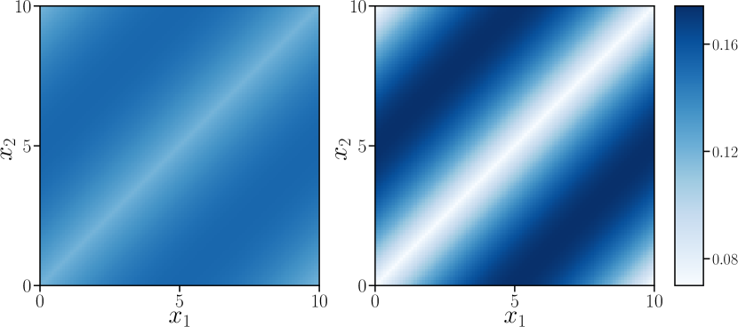
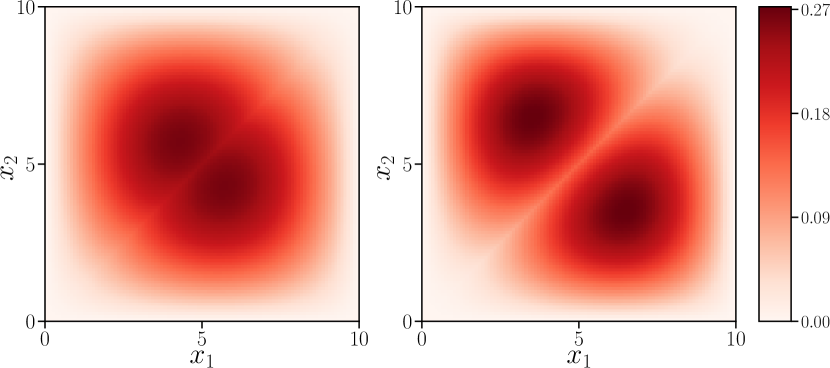
Figure 1: The normalized ground-state wavefunctions of $N=2$ particles in the LL model under periodic boundary condition (upper row) and hard-wall boundary condition (lower row) with the increasing interaction strength $c$ from left to right in each row. One can see how different geometries defined by boundary conditions are reflected in the wavefunction profiles. When $c$ is small, the two particles are more likely to share a common space, while they move away from each other as $c$ increases. Between the two extreme regimes of $c$, i.e., $c=0$ and $c=\infty$, there appears a maximum sensitivity of the wavefunction with respect to $c$, which is reflected in the larger Fisher information in that region which we reveal below.

The most well-known solution of the LL model is the one under the periodic boundary condition describing the one-dimensional system of $N$ bosons moving along a ring. The Bethe ansatz for this boundary condition is given by

$$\tilde{\psi}(x_{1},\cdots,x_{N})=\sum_{P^{\prime}s}A(P)\,e^{\,i\sum_{j=1}^{N}k_{P_{j}}x_{j}}\,,$$ (3)

where the continuity equation gives

$$A(P)=\prod_{j<l}\bigg{(}1+\frac{ic}{k_{P_{j}}-k_{P_{l}}}\bigg{)}.$$

The tilde of $\tilde{\psi}$ in Eq. (3) emphasizes that it is unnormalized. The sum over $P$’s means the sum over a set of the permutations of the integers from 1 to $N$. The energy and the momentum of the state described by this wavefunction are $E_{N}=\sum_{j=1}^{N}k_{j}^{2}$ and $P_{N}=\sum_{j=1}^{N}k_{j}$, respectively. Then applying the periodic boundary condition introduces the system size $L$ by imposing the cyclicity condition on the wavefunction, i.e., $\tilde{\psi}(x_{1},\cdots,x_{N})=\tilde{\psi}(x_{2},\cdots,x_{N},x_{1}+L)$, which is now defined in the domain $D^{\prime}:0<x_{1}<\cdots<x_{N}<L$. From this condition, one obtains a system of $N$ equations, i.e., Bethe equations:

$$Lk_{j}=2\pi I_{j}-2\sum_{l=1}^{N}\tan^{-1}\!\Big{(}\frac{k_{j}-k_{l}}{c}\Big{)},$$ (4)

which relates the quasi-momenta $k_{j}$’s to the values of $I_{j}$’s given $c$ and $L$. The quantum numbers, $I_{1}<I_{2}<\cdots<I_{N}$, are half-integers for even $N$ or integers for odd $N$ and do not allow duplicate values. The symmetric distribution of $I_{j}$’s around $0$ with interval $1$, i.e., $[I_{1}=-(N-1)/2,I_{2}=-(N-3)/2,\cdots,I_{N}=(N-1)/2]$, gives the symmetric distribution of $k_{j}$’s around $0$, which obviously minimizes the energy. Thus it corresponds to the ground state with minimal energy and zero momentum. The norm of the unnormalized wavefuction in Eq. (3) has been conjectured in Ref. [10] and proved in Ref. [49] using the method of algebraic Bethe ansatz. The norm squared of Eq. (3) has thus been established to be

$$\mathcal{N}^{\,2}=\prod_{j<l}\Big{(}1+\frac{c^{2}}{(k_{j}-k_{l})^{2}}\Big{)}\,\text{det}[\mathbf{H}]\,,$$ (5)

where the matrix $\mathbf{H}$ is

$$[\mathbf{H}]_{ij}=\delta_{ij}\Big{(}L+\sum_{l=1}^{N}\frac{2c}{(k_{i}-k_{l})^{2}+c^{2}}\Big{)}-\frac{2c}{(k_{i}-k_{j})^{2}+c^{2}}\,.$$

The LL model with the hard-wall boundary condition has been covered in Refs. [6, 8, 9, 10, 11]. The Bethe ansatz for this boundary condition is given by

$$\tilde{\psi}(x_{1},\cdots,x_{N})=\sum_{\epsilon^{\prime}s}\sum_{P^{\prime}s}\,\pi_{\epsilon}\,A(\epsilon,P)\,e^{i\sum_{j=1}^{N}\epsilon_{j}k_{P_{j}}x_{j}}\,,$$ (6)

where the continuity equation gives

$$A(\epsilon,P)=\prod_{j<l}\Big{[}1-\frac{i\,c}{\epsilon_{j}k_{P_{j}}+\epsilon_{l}k_{P_{l}}}\Big{]}\Big{[}1+\frac{i\,c}{\epsilon_{j}k_{P_{j}}-\epsilon_{l}k_{P_{l}}}\Big{]}.$$ (7)

Here, $\epsilon:=\{\epsilon_{1},\cdots,\epsilon_{N}\}$ and each $\epsilon_{j}$ is summed over $\pm 1$. The $P$ runs over all permutations of $[1,2,\cdots,N]$ as in Eq. (3) and $\pi_{\epsilon}$ is the product of all $\epsilon_{j}$’s: $\epsilon_{1}\epsilon_{2}\cdots\epsilon_{N}$. The sign of $k_{j}$ is absorbed into $\epsilon_{j}$ to make $k_{j}>0$ for all $j$’s and $k_{1}<k_{2}<\cdots<k_{N}$ is assumed without loss of generality due to the sum over $P$. The application of the hard-wall boundary condition introduces the system size $L$ by imposing a condition on the wavefunction, i.e., $\tilde{\psi}(x_{1}=0,x_{2},\cdots,x_{N})=\tilde{\psi}(x1,\cdots,x_{N-1},x_{N}=L)=0$, which is now defined in the domain $D^{\prime}$. This condition finally gives the Bethe equations for quasi-momenta:

$$Lk_{j}=\pi I_{j}-\sum_{l\neq j}\Big{[}\tan^{-1}\!\Big{(}\frac{k_{j}-k_{l}}{c}\Big{)}+\tan^{-1}\!\Big{(}\frac{k_{j}+k_{l}}{c}\Big{)}\Big{]}.$$ (8)

The quantum numbers, $I_{1}<I_{2}<\cdots<I_{N}$, are positive integers irrespective of the evenness of $N$ and do not allow duplicate values, thus the ground state corresponds to $[I_{1}=1,I_{2}=2,\cdots,I_{N}=N]$, which minimizes the energy $E_{N}=\sum_{j=1}^{N}k_{j}^{2}$. Applying the conjecture about the norm of Bethe ansatz in Ref. [10] to Eq. (8) leads to the norm squared of Eq. (6) that is expressible as Eq. (32) in the Appendix.

The LL model under either of the boundary conditions above is fully described by three parameters: interaction strength $c$, system size $L$, and particle number $N$. If one considers, however, the dimensionless form of LL model, i.e., $k_{j}\rightarrow\tilde{k_{j}}=L\,k_{j}$, $c\rightarrow\tilde{c}=c\,L$, and $x_{j}\rightarrow\tilde{x_{j}}=x_{j}/L$, one can find that the system depends only on the two parameters: $c\,L$ and $N$. Basically this origins from the characteristics of Bethe equations, Eq. (4) and Eq. (8), that for fixed $N$ the Bethe equations are invariant under any change of $c$ and $L$ keeping $c\,L$ constant. Hence for a fixed number of particles, the value of $\tilde{c}=c\,L$ completely determines the value of $\tilde{k}_{j}=Lk_{j}$ and thus the system. In thermodynamic limit, i.e., $N\rightarrow\infty$ with $N/L$ fixed, the LL model is completely described by a single parameter called Lieb’s parameter: $\gamma=c/\rho$, where $\rho$ is the number density $N/L$. Also, in this limit, the different effects between the two boundary conditions disappear and even the properties of bosonic gas along the ring space can be considered as if the gas resides in a flat box potential.

Though dimensionless form helps understand the essence of a system irrespective of the unit choice for the parameters, in order to test and apply the Fisher information as a realistic indicator for the limit of measurement precision, we don’t take such dimensionless parameters so that $c$ and $L$ can be treated separately. By doing so, we can verify how the independent adjustment of one parameter can help improve the measurement precision of the other, thus we can simulate the situations encountered in the real measurements. Also, we don’t assume thermodynamic limit and keep small number of particles to investigate the role of different geometries specified by different boundary conditions: periodic and hard-wall boundary conditions. Hence the system is now described by three independent parameters: $c$, $L$, and $N$.

III Fisher Information in the Lieb-Liniger Model

III.1 Fisher information of the wavefunction

The Fisher information has played an important role in the parameter estimation theory in that it determines the precision to which one can fundamentally estimate a parameter encoded in a probability distribution. For any conditional probability density $P(X|\theta)$ of a continuous random variable $X$, the CFI of a parameter $\theta$ is

$$F(\theta)=\int\!dx\,\frac{1}{P(x|\theta)}\Big{(}\frac{\partial P(x|\theta)}{\partial\theta}\Big{)}^{\!2}\,,$$ (9)

where the integral (or sum for a discrete random variable) is done over the domain of single measurement result $x$. The $F(\theta)$ quantifies how well two slightly different values of $\theta$ can be distinguished based on a single measurement outcome $x$. When a set of $M$ outcomes from $M$ independently and identically repeated measurements is used to estimate the $\theta$, the inverse of $\sqrt{MF(\theta)}$ provides the lower limit of estimation error as in Eq. (1).

In quantum theory, a quantum state parametrized by a parameter $\theta$ is connected to a probability distribution of the measurement results by $P(x|\theta)=\text{Tr}[\rho_{\theta}\hat{E}_{x}]$, where $\rho_{\theta}$ is the quantum state and a set of $\hat{E}_{x}$’s for all possible $x$’s, i.e., $\{\hat{E}_{x}:x\}$, is the positive operator-valued measure (POVM) specifying the type of measurement. Given $\rho_{\theta}$, the $\text{Tr}[\rho_{\theta}\hat{E}_{x}]$ allows additional optimization over the POVMs in a way that $F(\theta)$ is maximized. The maximal $F(\theta)$ defines the QFI of $\theta$:

$$\mathfrak{F}(\theta)=\max_{\{\hat{E}_{x}:x\}}\!F(\theta)=\text{Tr}[\rho_{\theta}L_{\theta}^{2}]\,,$$ (10)

where $L_{\theta}$ is the symmetric logarithmic derivative satisfying $\partial_{\theta}\rho_{\theta}=(\rho_{\theta}L_{\theta}+L_{\theta}\rho_{\theta})/2$. By Eq. (1), the QFI specifies the precision one can ultimately attain for estimating an unknown parameter encoded in a quantum state. Note that the optimal POVM making $F(\theta)$ reach its maximum can always be found. When the parameter $\theta$ is encoded by a unitary process with some generator $\hat{G}$, i.e., $\rho_{\theta}=e^{-i\theta\hat{G}}\rho_{0}\,e^{i\theta\hat{G}}$, the upper bound of QFI is given as $4\langle\psi_{0}|(\Delta G)^{2}|\psi_{0}\rangle$, which obviously can be reached when $\rho_{0}$ is a pure state: $\rho_{0}=|\psi_{0}\rangle\langle\psi_{0}|$. Thus, for general states including mixed ones, $\mathfrak{F}(\theta)\leq 4\langle\psi_{0}|(\Delta G)^{2}|\psi_{0}\rangle$ [28].

Here, however, we are concerned with the Fisher information of a Hamiltonian parameter that a quantum state naturally has after being realized as an eigenstate of that Hamiltonian rather than unitarily encoded. For the generic pure state $|\psi_{\theta}\rangle$ with $\theta$ encoded via a physical process, the QFI defined in (10) reduces to

$$\!\!\!\!\!\!\!\!\!\!\mathfrak{F}(\theta) = 4\,\Big{(}\langle\partial_{\theta}\psi_{\theta}|\partial_{\theta}\psi_{\theta}\rangle-\big{|}\langle\psi_{\theta}|\partial_{\theta}\psi_{\theta}\rangle\big{|}^{2}\Big{)}$$ (11)

$$= 4\,\Big{(}\!\int\!\!d\mathbf{x}\,\big{|}\partial_{\theta}\psi_{\theta}(\mathbf{x})\big{|}^{2}\!\!-\big{|}\!\!\int\!\!d\mathbf{x}\,\psi_{\theta}^{\ast}(\mathbf{x})\,\partial_{\theta}\psi_{\theta}(\mathbf{x})\big{|}^{2}\Big{)},$$

where it is also expressed in the position representation with an $N$-particle position state $|\mathbf{x}\rangle:=|x_{1},x_{2},\cdots,x_{N}\rangle$ satisfying $\int\!d\mathbf{x}|\mathbf{x}\rangle\langle\mathbf{x}|=\hat{1}$ and $\langle\mathbf{x}|\mathbf{x}^{\prime}\rangle=\delta(\mathbf{x}-\mathbf{x}^{\prime})$. When $\psi_{\theta}(\mathbf{x})$ is the most general complex-valued function, we can consider the polar representation of a wavefunction: $\psi_{\theta}(\mathbf{x})=|\psi_{\theta}(\mathbf{x})|e^{i\varphi_{\theta}(\mathbf{x})}$, with some real-valued function $\varphi_{\theta}(\mathbf{x})$. Then $\mathfrak{F}(\theta)$ in (11) can be further tranformed into

$$\frac{\mathfrak{F}(\theta)}{4}= \int\!\!d\mathbf{x}\,\big{(}\partial_{\theta}|\psi_{\theta}(\mathbf{x})|\big{)}^{2}+\int\!\!d\mathbf{x}\,|\psi_{\theta}(\mathbf{x})|^{2}\big{(}\partial_{\theta}\varphi_{\theta}(\mathbf{x})\big{)}^{2}$$ (12)

$$\qquad\qquad\qquad-\,\,\Big{(}\!\int\!\!d\mathbf{x}\,|\psi_{\theta}(\mathbf{x})|^{2}\,\partial_{\theta}\varphi_{\theta}(\mathbf{x})\Big{)}^{\!2},$$

where $\int\!d\mathbf{x}\,|\psi_{\theta}(\mathbf{x})|\,\partial_{\theta}|\psi_{\theta}(\mathbf{x})|=0$ derived from the $\theta$-derivative of $\int\!d\mathbf{x}\,|\psi_{\theta}(\mathbf{x})|^{2}=1$ is used. The second and third terms in (12) combine to be the variance of $\partial_{\theta}\varphi_{\theta}(\mathbf{x})$ with respect to the probability distribution $P(\mathbf{x}|\theta)=|\psi_{\theta}(\mathbf{x})|^{2}$. On the other hand, the CFI in (9) can be recast in terms of the wavefunction by the relation $P(\mathbf{x}|\theta)=|\psi_{\theta}(\mathbf{x})|^{2}$:

$$F(\theta)=4\!\int\!d\mathbf{x}\,\big{(}\partial_{\theta}|\psi_{\theta}(\mathbf{x})|\big{)}^{\!2}\,,$$ (13)

and finally it obviously follows that the QFI in Eq. (12) comprises two parts [50, 51]:

$$\mathfrak{F}(\theta)=F(\theta)+4\,\text{Var}\big{[}\partial_{\theta}\varphi_{\theta}\big{]}_{\psi_{\theta}}\,,$$ (14)

in which $\text{Var}[A]_{\psi_{\theta}}$ means the variance of a quantity $A(\mathbf{x})$ with respect to the probability distribution $|\psi_{\theta}(\mathbf{x})|^{2}$.

To represent the CFI in terms of the wavefunction implies that a set of $\hat{E}_{\mathbf{x}}=|\mathbf{x}\rangle\langle\mathbf{x}|$, i.e., $\{|\mathbf{x}\rangle\langle\mathbf{x}|:\mathbf{x}\}$, is chosen as a POVM, which means the projective measurement of the positions of $N$ particles. This POVM is not optimal according to Eq. (14), but we can find it optimal under certain conditions. One notable case is when $\psi_{\theta}(\mathbf{x})=e^{i\varphi(\theta)}\phi_{\theta}(\mathbf{x})$ with $\varphi(\theta)$ and $\phi_{\theta}(\mathbf{x})$ being real-valued. Since $\varphi(\theta)$ is independent of $\mathbf{x}$, the variance term in Eq. (14) disappears, hence $\mathfrak{F}(\theta)=4\int d\mathbf{x}\,(\partial_{\theta}\phi_{\theta}(\mathbf{x}))^{2}=F(\theta)$. For example, if $\psi_{\theta}(\mathbf{x})$ is real-valued, i.e., $\varphi(\theta)=0$, or is purely imaginary-valued, i.e., $\varphi(\theta)=\pi/2$, the QFI will be $4\int d\mathbf{x}\,(\partial_{\theta}\psi_{\theta}(\mathbf{x}))^{2}$ or $-4\int d\mathbf{x}\,(\partial_{\theta}\psi_{\theta}(\mathbf{x}))^{2}$, respectively, which is exactly equal to the CFIs calculated by Eq. (13) with the corresponding $\psi_{\theta}(\mathbf{x})$. If $\phi_{\theta}(\mathbf{x})$ is an eigenstate of a Hamiltonian, which can always be chosen to be real, then $e^{i\varphi(\theta)}\phi_{\theta}(\mathbf{x})$ is a representation of its time evolution, where $\varphi_{\theta}$ contains the eigenenergy of the state that also relies on the Hamiltonian parameter $\theta$. Thus the saturation of CFI to QFI is maintained along the time evolution. Finally, the Fisher information defined as above applies to the case when one tries to estimate a Hamiltonian parameter $\theta$ from the position measurement on the eigenstates of that Hamiltonian.

III.2 Single-shot measurement with finite resolution

The ultimate quantum limit of any measurement precision is identified by the QFI, but the feasible limit is always given by the CFI, that is, by a specific choice of measurement. Relating the probability density $P(x|\theta)$ to the wavefunction $\psi_{\theta}(x)$ introduces a (hypothetical) measurement where the positions of $N$ particles are determined with infinite level of precision. Even though we have discussed the condition on $\psi_{\theta}(x)$ to make $\mathfrak{F}(\theta)=F(\theta)$, what one actually encounters in the real experiments is the imperfect measurement allowing for uncertainty in the measured positions, which can be supported by the absorption imaging method that has been used as a measurement to investigate the cold atomic systems [52]. This method is implemented by irradiating laser light from above to the cold atomic gas and measuring the brightness captured by the CCD camera installed below the gas. The brightness profile generated from the camera is fitted to obtain the column density distribution of the gas, hence this absorption imaging is thought of as a measurement of the number of particles in each pixel area of the camera. Then one can estimate any system parameter from the density profile. By using a model of single-shot measurement with finite resolution to simulate the absorption imaging [53, 54, 55], it can be shown that as narrowing the pixel size, one can asymptotically obtain the precision level provided by the perfect position measurement.

The imperfect measurement of the position of a single particle in one-dimensional space with finite resolution $\Delta x_{p}$ is described by the POVM $\{\hat{\Pi}_{j}:j\}$ satisfying

$$\hat{\Pi}_{j}:=\!\int_{a_{j}}^{a_{j+1}}\!\!\!\!\!\!\!\!dx\,\hat{\Pi}(x)\,,\,\,\,\,\sum_{j}\hat{\Pi}_{j}=\!\int_{-\infty}^{\infty}\!\!\!\!dx\,\hat{\Pi}(x)=\mathbb{I}\,,$$ (15)

where $\hat{\Pi}(x)=|x\rangle\langle x|$ forms a POVM for the perfect position measurement and $a_{j+1}-a_{j}=\Delta x_{p}$ for all $j$’s. It is easy to show that $\hat{\Pi}_{j}\,\hat{\Pi}_{l}=\delta_{jl}$, which is the property satisfied by the projective measurements. Thus the probability of finding a particle within a range $(a_{j},a_{j+1})$, i.e., $\text{Tr}[\rho_{\theta}\hat{\Pi}_{j}]$, is considered instead of the one of finding the particle exactly at $x$, i.e., $\text{Tr}[\rho_{\theta}\hat{\Pi}(x)]dx$, for a given quantum state $\rho_{\theta}$.

We extend this consideration to the case of $N$ particles and $N_{p}$ pixels. The coordinate range of $j$th pixel is denoted by $A_{j}:=(a_{j-1},a_{j})$, where $j=0,1,\cdots,N_{p},N_{p}+1$ and $a_{j}-a_{j-1}=\Delta x_{p}$ for all $j$’s except for $0$ and $N_{p}+1$. Also, we define $a_{-1}:=-\infty$ and $a_{N_{p}+1}:=\infty$. A one-dimensional absorption image can be written as $\mathfrak{n}:=(\mathfrak{n}_{0},\mathfrak{n}_{1},\cdots,\mathfrak{n}_{N_{p}},\mathfrak{n}_{N_{p}+1})$, where $\mathfrak{n}_{j\neq 0,N_{p}+1}$ is the number of atoms found in $j$th pixel bin and $\sum_{j=0}^{N_{p}+1}\mathfrak{n}_{j}=N$, i.e., the total number of particles. We assume the length $\Delta x_{p}N_{p}$ should be large enough to cover the whole system, but the numbers of atoms outside the measured area, $\mathfrak{n}_{0}$ for the left and $\mathfrak{n}_{N_{p}+1}$ for the right, are considered for theoretical completion.

Now one can think of the probability distribution of absorption images:

$$P(\mathfrak{n}|\theta)=\zeta_{\mathfrak{n}}\!\!\int_{A}\!d\mathbf{x}\,P(\mathbf{x}|\theta)\,,\sum_{\mathfrak{n}\in H(N,N_{p})}\!\!\!\!\!\!P(\mathfrak{n}|\theta)=1\,,$$ (16)

where $P(\mathbf{x}|\theta)$ is obtained from the absolute-square of $N$-particle wavefunction, i.e., $|\psi_{\theta}(\mathbf{x})|^{2}$, and

$$\zeta_{\mathfrak{n}}:=\frac{N!}{\prod_{j=0}^{N_{p}+1}\mathfrak{n}_{j}!}\,,\,\,\int_{A}d\mathbf{x}:=\int_{A_{j_{1}}}\!\!\!\!dx_{1}\int_{A_{j_{2}}}\!\!\!\!dx_{2}\,\cdots\int_{A_{j_{N}}}\!\!\!\!\!\!dx_{N}\,.$$

Also, $H(N,N_{p})$ is a set of the different ways of selecting $N$ elements out of $\{A_{j}:j=0,1,\cdots,N_{p}+1\}$ allowing for duplication, i.e., a set of all absorption images that can be realized. The integration part gives the probability of finding the 1st particle in the range $A_{j_{1}}$, the 2nd particle in the range $A_{j_{2}}$, and so on. Note that the set $A=\{A_{j_{1}},\cdots,A_{j_{N}}\}$ is in an ascending order, i.e., $j_{1}\leq j_{2}\leq\cdots\leq j_{N}$, and that’s why $\zeta_{\mathfrak{n}}$ is multiplied to consider the indistinguishability of particles. In short, the $A$ is an area in the $N$-dimensional space of $(x_{1},\cdots,x_{N})$, where any element leads to the same absorption image, i.e., $\mathfrak{n}$. Finally, using Eq. (16), the CFI for the absorption imaging is obtained as

$$F(\theta)\quad=\sum_{\mathfrak{n}\in H(N,N_{p})}\frac{1}{P(\mathfrak{n}|\theta)}\Big{(}\frac{dP(\mathfrak{n}|\theta)}{d\theta}\Big{)}^{2}\,,$$ (17)

which determines the precision level for estimating $\theta$ of $\rho_{\theta}$ from the results of absorption imaging method.

For example, let us suppose $N=10$ and $N_{p}=3$, that is, 10 particles and 3 pixels, thus a case of very low resolution. Then the integration area, i.e., $A$, corresponding to an absorption image $\mathfrak{n}=(1,5,1,3,0)$ will be $\{A_{0},A_{1},A_{1},A_{1},A_{1},A_{1},A_{2},A_{3},A_{3},A_{3}\}$ and $\zeta_{\mathfrak{n}}=10!/(1!5!1!3!0!)=5040$. Like this, any absorption image has a corresponding representation of $A$. The probability of attaining $(1,5,1,3,0)$ as an absorption image can be calculated as

$$5040\times\!\!\int_{-\infty}^{a_{0}}\!\!\!\!dx_{1}\int_{a_{0}}^{a_{1}}\!\!\!\!dx_{2}\int_{a_{0}}^{a_{1}}\!\!\!\!dx_{3}\cdots\!\!\int_{a_{2}}^{a_{3}}\!\!\!\!dx_{10}\,P(\mathbf{x}|\theta)\,,$$

where $P(\mathbf{x}|\theta)=|\psi_{\theta}(\mathbf{x})|^{2}$ and the integral about each range is implemented with the repetition indicated by $(1,5,1,3,0)$. Also, $H(N,N_{p})$ is a set of all absorption images that can be realized by $10$ particles with $3+2$ ranges:

$$\{(10,0,0,0,0),(9,1,0,0,0),\cdots(0,0,0,0,10)\}$$

with the total number of elements $\frac{(N+N_{p}+1)!}{(N_{p}+1)!N!}=1001$. Now we have everything in hand to calculate the CFI for the absorption imaging. Later on, we will check by numerical simulation that the CFI of the single-shot measurement with finite resolution, i.e., Eq. (17), converges to the CFI provided by the wavefuction, i.e., Eq. (13), as narrowing $\Delta x_{p}$.

III.3 Fisher information of the Bethe ansatz

We suppose that the interaction strength $c$ is a target parameter to be estimated and the system size $L$ is a known resource parameter that we can directly control in the LL model. The $L$ is a resource in a sense that it serves a possibility of enhancing measurement precision of another parameter $c$. Note that we focus on the estimation of a Hamiltonian parameter that is encoded into a state while it is being realized as an eigenstate of the Hamiltonian rather than by evolving through a unitary evolution, e.g., Mach-Zehnder or Ramsey interferometry. Hence we use Eq. (11) and Eq. (13) in Sec. III.1 to calculate the QFI and the CFI directly from the wavefunctions. Since the wavefunctions in Eq. (3) and Eq. (6) are unnormalized, the expressions of QFI and CFI, i.e., Eq. (11) and Eq. (13), need to be rewritten in terms of unnormalized wavefunctions:

$$\mathfrak{F}=\frac{4}{\mathcal{N}^{2}}\bigg{[}\!\int\!d\mathbf{x}\,\Big{|}\frac{d\tilde{\psi}}{dc}\Big{|}^{2}\!\!-\frac{1}{\mathcal{N}^{2}}\Big{|}\!\int\!d\mathbf{x}\,\tilde{\psi}^{\ast}\frac{d\tilde{\psi}}{dc}\Big{|}^{2}\bigg{]},$$ (18a)

$$F=\frac{4}{\mathcal{N}^{2}}\bigg{[}\!\int\!d\mathbf{x}\,\Big{(}\frac{d|\tilde{\psi}|}{dc}\Big{)}^{\!2}\!\!-\Big{(}\frac{d\mathcal{N}}{dc}\Big{)}^{\!2}\bigg{]}.$$ (18b)

If $\tilde{\psi}$ is a normalized wavefunction, i.e., $\mathcal{N}=1$, then Eq. (11) and Eq. (13) are recovered.

The expansion of QFI with respect to the Bethe ansatz solution under periodic boundary condition, i.e., Eq. (3), is the following:

$$\mathfrak{F}_{p}=\frac{4}{\mathcal{N}^{2}}\Bigg{[}\,\, \sum_{P,Q}\bigg{(}\frac{dA^{\ast}(P)}{dc}\frac{dA(Q)}{dc}\,\mathfrak{I}(k_{P}-k_{Q})+i\,\frac{dA^{\ast}(P)}{dc}A(Q)\sum_{l=1}^{N}\frac{dk_{Q_{l}}}{dc}\,\mathfrak{I}_{l}^{1}(k_{P}-k_{Q})$$ (19)

$$\qquad\quad\;\;\,-\,\,i\,A^{\ast}(P)\frac{dA(Q)}{dc}\sum_{l=1}^{N}\frac{dk_{P_{l}}}{dc}\,\mathfrak{I}_{l}^{1}(k_{P}-k_{Q})+A^{\ast}(P)A(Q)\!\!\!\sum_{m,n=1}^{N}\!\!\frac{dk_{P_{m}}}{dc}\frac{dk_{Q_{n}}}{dc}\,\mathfrak{I}_{mn}^{11}(k_{P}-k_{Q})\bigg{)}$$

$$\,\,-\,\,\frac{1}{\mathcal{N}^{2}}\,\bigg{|}\sum_{P,Q}\Big{(}A^{\ast}(P)\frac{dA(Q)}{dc}\,\mathfrak{I}(k_{P}-k_{Q})+i\,A^{\ast}(P)A(Q)\sum_{l=1}^{N}\frac{dk_{Q_{l}}}{dc}\,\mathfrak{I}_{l}^{1}(k_{P}-k_{Q})\Big{)}\bigg{|}^{2}\Bigg{]},$$

where a notation

$$\mathfrak{I}_{mn}^{\alpha\beta}(\lambda):=\int_{0}^{L}\!\!\!dx_{N}\int_{0}^{x_{N}}\!\!\!\!\!\!dx_{N-1}\cdots \int_{0}^{x_{2}}\!\!\!\!dx_{1}\,x_{m}^{\alpha}\,x_{n}^{\beta}$$ (20)

$$e^{-i\sum_{j=1}^{N}\lambda_{j}x_{j}}\,,$$

is introduced to abbreviate similarly repetitive integrals and the indices of $\mathfrak{I}$ are the integers satisfying $1\leq m,n\leq N$ and $\alpha,\beta\geq 0$. Also, $x_{m}^{\alpha}$ ($x_{n}^{\beta}$) means $x_{m}$ ($x_{n}$), i.e., the position of $m$th ($n$th) particle, to the power of $\alpha$ ($\beta$) and if the each power, i.e., $\alpha$ or $\beta$, is zero, then the corresponding subscript, i.e., $m$ or $n$, needs not be specified, thus it can be omitted. The $\lambda$ in Eq. (20) indicates $\{\lambda_{1},\cdots,\lambda_{N}\}$ and likewise, $k_{P}$ and $k_{Q}$ are the short notations for the permuted set of quasi-momenta, i.e., $(k_{P_{1}},\cdots,k_{P_{N}})$ and $(k_{Q_{1}},\cdots,k_{Q_{N}})$, repectively. Hence all of $\mathfrak{I}(k_{P}-k_{Q})$, $\mathfrak{I}_{l}^{1}(k_{P}-k_{Q})$, and $\mathfrak{I}_{mn}^{11}(k_{P}-k_{Q})$ in Eq. (19) are clearly defined.

The replacement of $\sum_{P,Q}\rightarrow\sum_{\epsilon,\delta}\pi_{\epsilon}\pi_{\delta}\sum_{P,Q}$, $A(P)\rightarrow A(\epsilon,P)$, $A(Q)\rightarrow A(\delta,Q)$, $k_{P_{j}}\rightarrow\epsilon_{j}k_{P_{j}}$, and $k_{Q_{j}}\rightarrow\delta_{j}k_{Q_{j}}$, and modifying the definition of $\mathcal{N}$ from Eq. (5) to Eq. (32) lead to the corresponding QFI for the hard-wall boundary condition, i.e., $\mathfrak{F}_{h}$. Refer to Eq. (3) and Eq. (6) for the definitions of the replaced symbols above. The CFI in Eq. (18b) can be similarly expanded under each boundary condition.

In Eq. (19), it is obvious from the definitions that $\mathcal{N}$, $A(P)$, $A(Q)$, and the multiple integral parts all depend on the difference between any two quasi-momenta in $\{k_{1},k_{2},\cdots,k_{N}\}$, not on the values of quasi-momenta themselves. Furthermore, from the Bethe equations in Eq. (4) under the periodic boundary condition, we can derive the following analytical expression for the derivative of quasi-momenta with respect to $c$:

$$\frac{dk_{j}}{dc}=\sum_{a=1}^{N}\big{[}\mathbf{H}^{-1}\big{]}_{ja}\sum_{l=1}^{N}\frac{2(k_{a}-k_{l})}{c^{2}+(k_{a}-k_{l})^{2}}\,,$$ (21)

where the matrix $\mathbf{H}$ is from Eq. (5) and relies on the difference between any two quasi-momenta. This shows that $dk_{P_{j}}/dc$ or $dk_{Q_{j}}/dc$ in Eq. (19) also depends on a set of $N-1$ elements $\{k_{1}-k_{2},k_{2}-k_{3},\cdots,k_{N-1}-k_{N}\}$, not on $\{k_{1},k_{2},\cdots,k_{N}\}$. The $dA(P)/dc$ and $dA(Q)/dc$ are functions of $\{k_{1}-k_{2},k_{2}-k_{3},\cdots,k_{N-1}-k_{N}\}$, thus the QFI in Eq. (19) is a function of $k_{j}-k_{j+1}$ for all $j$’s. This implies that $\mathfrak{F}_{p}$ and $F_{p}$ are invariant under the translation of whole quantum numbers: $\{I_{1},\cdots,I_{N}\}\rightarrow\{I_{1}+J,\cdots,I_{N}+J\}$. The sum over permutations, i.e., $\sum_{P}\sum_{Q}$, makes $\mathfrak{F}_{p}$ and $F_{p}$ invariant under the reverse of $\{k_{1}-k_{2},k_{2}-k_{3},\cdots,k_{N-1}-k_{N}\}$, too. An example for this case is a transition from a state with quantum numbers $[-1,0,2]$ to a state with $[-1,1,2]$.

On the other hand, under the hard-wall boundary condition, the derivative of Bethe equations in Eq. (8) gives

$$\!\!\!\!\!\!\!\!\!\!\frac{dk_{j}}{dc}= \,\sum_{a=1}^{N}\big{[}\mathbf{H}^{-1}\big{]}_{ja}$$ (22)

$$\,\,\,\,\times\sum_{l\neq a}\Big{[}\frac{k_{a}-k_{l}}{c^{2}+(k_{a}-k_{l})^{2}}+\frac{k_{a}+k_{l}}{c^{2}+(k_{a}+k_{l})^{2}}\Big{]},$$

where the matrix $\mathbf{H}$ is from Eq. (32). This means that the QFI and the CFI for the hard-wall geometry depend on both of $\{k_{j}-k_{j+1}|j=1,2,\cdots,N-1\}$ and $\{k_{j}+k_{j+1}|j=1,2,\cdots,N-1\}$, i.e., $\{k_{j}|j=1,2,\cdots,N\}$. Thus there’s no invariance of $\mathfrak{F}_{h}$ and $F_{h}$ with respect to the above operations on quantum numbers.

There are several difficulties in the calculation of QFI and CFI with respect to the LL eigenstates. One of them is that we encounter computing the multiple integrals in the domain $D^{\prime}$ as in Eq. (20). These multiple integrals appear in the calculation of the norm, scalar product [56, 57, 58], and correlation function [59] with respect to the Bethe ansatz. Using the simple calculative techniques specified in Ref. [59]

$$\int\!dx\,x^{p}\,e^{ikx}=-p!\,\Big{(}\frac{i}{k}\Big{)}^{p+1}\!\!e^{ikx}\sum_{s=0}^{p}\frac{(-ikx)^{s}}{s!}\,,$$

we can reduce the computational time when compared to purely letting the integrals be implemented by Monte-Carlo simulation. Another severe issue arises in the sums which are inherent in the Bethe ansatz: $(\sum_{P})^{2}$ or $(\sum_{\epsilon}\sum_{P})^{2}$ for the periodic or hard-wall boundary conditions, respectively. This results in a huge algorithmic complexity proportional to $\sim N!^{2}$ or $\sim 2^{2N}N!^{2}$ for each boundary condition. To avoid this complexity, we restrict ourselves to a small number of particles in the numerical calculation of Fisher information.

IV Analysis of the Fisher information

Since the CFI based on a wavefunction is expected to be attainable by the absorption imaging method, which is later shown, we calculate the QFI and the CFI for the interaction strength $c$ imprinted on the eigenfunctions of the LL Hamiltonian to see how precisely the parameter can be determined by implementing the single-shot measurement on the LL stationary states. We investigate how under different boundary conditions the Fisher information for $c$ behaves according to the system variables, e.g., $c$, $L$, and $N$, and the types of low-lying elementary excitations. The Fisher information is numerically computed by Eq. (19) and its adjusted version for the hard-wall boundary condition.

IV.1 Ground states

First we examine the case of the LL ground states that have the least number of interacting particles, i.e., $N=2$. Under the periodic boundary condition, the quantum numbers for the ground state, i.e., $[I_{1}=-1/2,I_{2}=1/2]$, lead to symmetrically distributed quasi-momenta, i.e., $k_{2}=-k_{1}$, which make the wavefunction in Eq. (3) real-valued. Under the hard-wall boundary condition, the set of quantum numbers for the ground state is $[I_{1}=1,I_{2}=2]$ and results in the corresponding quasi-momenta satisfying $0<k_{1}<k_{2}$. Due to the form of Bethe ansatz that has the wave components reflected from the hard-wall, the wavefunction in Eq. (6) is real-valued, too. In conclusion, the QFI and the CFI are completely equal for the $N=2$ LL ground states.

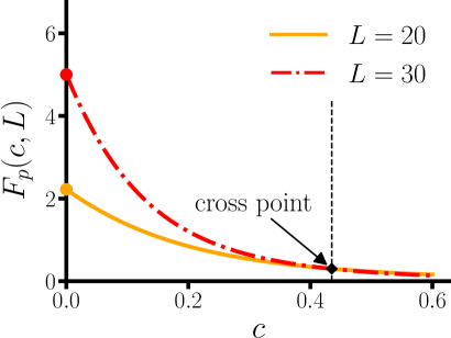
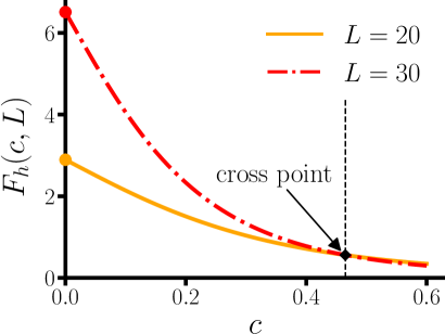
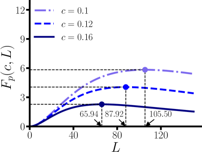
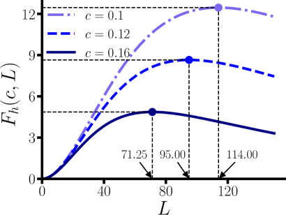
Figure 2: The CFI for $c$ of the $N=2$ LL ground state as a function of the system variables: $c$ and $L$. In each row, the left plot is for the periodic boundary condition and the right plot is for the hard-wall boundary condition. For $N=2$, both ground-state wavefunctions are real-valued, thus the CFI, i.e., $F(c,L)$, is equal to the QFI, i.e., $\mathfrak{F}(c,L)$. In the upper row, the maximum value at $c=0$ is $L^{2}/180\simeq 0.0056L^{2}$ for $F_{p}(c,L)$ and $L^{2}(-855+60\pi^{2}+4\pi^{4})/(180\pi^{4})\simeq 0.0072L^{2}$ for $F_{h}(c,L)$. In the lower row, the maximum points appear at $c\,L_{\text{max}}\simeq 10.55$ for $F_{p}(c,L)$ and $c\,L_{\text{max}}\simeq 11.40$ for $F_{h}(c,L)$. Hence, for larger $c$, the optimal system size $L_{\text{max}}$ appears at a smaller value. Also, note that the hard-wall geometry helps to enhance the Fisher information in excess of its ring-geometry counterpart.

The Fig. 2 shows how the CFI behaves according to $c$ (upper row) or $L$ (lower row) in the case above. In each row, the left plot shows the CFI for the periodic boundary condition, i.e., $F_{p}(c,L)$, and the right plot shows the CFI for the hard-wall boundary condition, i.e., $F_{h}(c,L)$, and they can be compared in parallel, with the same scales of axes.

In the upper row, we can see a rapid and monotonic decrement of CFI as the interaction coupling $c$ increases, exhibiting a maximum at $c=0$. Larger $L$ leads to higher CFI under the same value of $c$, but this is reversed after some value of $c$. Also, note that $F_{p}(c,L)\leq F_{h}(c,L)$. In the upper left plot, the maximum value can be computed as $F_{p}(c=0,L)=L^{2}/180\simeq 0.0056L^{2}$ by inserting the small-$c$ approximation $k_{j}=q_{j}\sqrt{2c/L}+O(c)$, where the $q_{j}$ are the zeroes of Hermite polynomial of order $N$, i.e., $H_{N}(q)$ [10], into the $F_{p}(c,L)$ and taking the limit $c\rightarrow 0$. In the upper right plot, $k_{1}=\pi/L-\sqrt{c/(2L)}+O(c)$ and $k_{2}=\pi/L+\sqrt{c/(2L)}+O(c)$ are inserted into $F_{h}(c,L)$, and then taking the limit $c\rightarrow 0$ gives $F_{h}(c=0,L)=L^{2}(-855+60\pi^{2}+4\pi^{4})/(180\pi^{4})\simeq 0.0072L^{2}$. When $c$ is extremely large, the quasi-momenta $k_{j}$’s are getting less relevant to the $c$ since $k_{j}\rightarrow 2\pi I_{j}/L$ or $k_{j}\rightarrow\pi I_{j}/L$ up to the first dominant term under the periodic or hard-wall boundary condition, thus the distinguishability of the ground state with respect to $c$ decreases.

The lower row in Fig. 2 shows the variation of CFI as the system size $L$ increases. Both of $F_{p}(c,L)$ and $F_{h}(c,L)$ rise from $0$ at $L=0$, reach their maxima at $L=L_{\text{max}}$, and finally decrease gradually. As mentioned, the CFI is a quadratic function of $L$ when $c=0$ and monotonically increases as $L\rightarrow\infty$. For any nonzero value of $c>0$, however, the region of the quadratic increase with $L$ of the CFI moves to a regime of smaller $L$, and the CFI begins to decrease after reaching a maximum at $L=L_{\text{max}}$, thus it is confirmed that the interaction overall deteriorates the measurement precision. The maximum of CFI gets lower as $c$ increases and its position $L_{\text{max}}$ moves to the left accordingly. We have numerically obtained this optimal value of $L$ by solving $dF_{p,h}(c,L)/dL|_{L=L_{\text{max}}}=0$: $c\,L_{\text{max}}\simeq 10.55$ for $F_{p}(c,L)$ and $c\,L_{\text{max}}\simeq 11.40$ for $F_{h}(c,L)$. In short, the optimal system size $L_{\text{max}}$ appears at a smaller value for a larger $c$. Here, we also note that $F_{p}(c,L)\leq F_{h}(c,L)$, where the maximal value of $F_{h}(c,L)$ is roughly two times larger than the one of $F_{p}(c,L)$ for the same $c$.

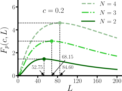
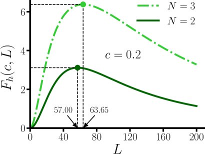
Figure 3: The CFI for $c$ of the LL ground state as a function of $L$, where $c=0.2$ and the particle number is slightly increased from $N=2$. The left plot is for the periodic boundary condition, in which the ground-state wavefunction is real-valued for all $N$. The right plot is for the hard-wall boundary condition, in which the ground-state wavefunction is real-valued for even $N$ or is purely imaginary-valued for odd $N$. In any case, the CFI is equal to the QFI. As $N$ grows, the CFI shows a significant enhancement over the whole range of $L$ maintaining its behavioral pattern and the $L_{\text{max}}$, at which the CFI is maximal, moves right: $c\,L_{\text{max}}\simeq 10.55,13.63,16.92$ for $F_{p}(c,L)$ and $c\,L_{\text{max}}\simeq 11.40,12.73$ for $F_{h}(c,L)$. For the same $N$, the system with hard-wall geometry exhibits a much higher CFI.

In most cases, the Fisher information is dependent on a target parameter, which leads to inhomogeneous estimation precision over the range of the target parameter. In other words, the precision that would be obtained if the true $\theta$ were $\theta_{1}$ can be larger or smaller than the one that would be attained if $\theta$ were a different value $\theta_{2}$. An exception to this is the estimation of the mean of a Gaussian distribution, where the Fisher information for the mean does not depend on the mean itself and is given by the inverse of the variance. Similarly, in Mach-Zehnder interferometry (MZI), one often tries to estimate the $\theta$ encoded by unitary operator, e.g., $e^{-i\theta\hat{\sigma}_{y}}$, to a general quantum state $\rho_{0}=(I+\vec{s}_{0}\cdot\vec{\sigma})/2$, where $\vec{s}_{0}\in\mathbf{R}^{3}$ with $|\vec{s}_{0}|\leq 1$ and $\vec{\sigma}$ is the vector of Pauli matrices, i.e., $\{\sigma_{x},\sigma_{y},\sigma_{z}\}$. The QFI in this case depends only on $\vec{s}_{0}$, but not on $\theta$, while the CFI for the measurement of population imbalance between two arms of interferometer, which is the typical choice in MZI, is dependent on $\theta$ as well as the initial state parameter $\vec{s}_{0}$. For pure states, there exists a class of optimal $\vec{s}_{0}$’s which lets the CFI saturate the QFI. See Refs. [37, 39] for further details. On the other hand, unlike the typical (linear) MZI above, where the parameter to be estimated appears as a multiplicative factor to the generator of unitary evolution, the dependence of a Hamiltonian on the parameter can be more general [60]. In this case, the QFI can rely on the target parameter itself. In the present example of LL model, the system size $L$ plays the role of initial state parameter other than the target parameter $c$, and the equality of QFI and CFI is guaranteed for the $N=2$ ground state. Here, the QFI for $c$ has the dependence on $c$ as in the metrology with the general Hamiltonian above, thus the optimal $L$, i.e., $L_{\text{max}}$, relies on the value of $c$, which is quite different from the linear MZI case. Also, our metrological protocol does not use any unitary operator to encode the target parameter and that is why the QFI does not have a cyclical property with respect to $c$ [39].

In Fig. 3, the particle number is raised up to $N=4$ in the case of $F_{p}(c,L)$ (left plot), while up to $N=3$ in the case of $F_{h}(c,L)$ (right plot), where $c=0.2$ is supposed in all plots. The wavefunction in Eq. (3) is real-valued for any $N$ if the quasi-momenta, i.e., $\{k_{1},k_{2},\cdots,k_{N}\}$, are symmetrically distributed around $0$ and the ground state satisfies this condition. On the other hand, the wavefunction in Eq. (6) is real-valued for even $N$ and purely imaginary-valued for odd $N$. Thus, as far as the ground-states are concerned, the CFI and the QFI are equal for any $N$. As $N$ increases, the CFI increases over the whole range of $L$ and the $L_{\text{max}}$ increases accordingly: $c\,L_{\text{max}}\simeq 10.55,13.63,16.92$ for $F_{p}(c,L)$ and $c\,L_{\text{max}}\simeq 11.40,12.73$ for $F_{h}(c,L)$. Also, the advantage of hard-wall geometry for the CFI is clear from the Fig. 3, when keeping $N$ fixed.

IV.2 Excited states

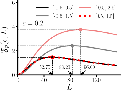
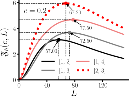
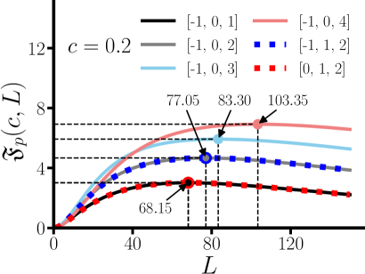
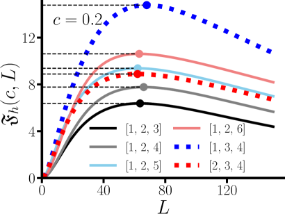
Figure 4: The QFI for $c$ of the LL ground or excited state as a function of $L$, where $c=0.2$. The upper row is for $N=2$ and the lower row is for $N=3$. In each row, the left plot is for the periodic boundary condition and the right plot is for the hard-wall boundary condition. Upper left) The type-I excited states give higher QFI as the energy increases, but the type-II excited state, i.e., $[0.5,1.5]$ (red dotted), gets back to the level of ground state, i.e., $[-0.5,0.5]$ (black solid). Upper right) The system with hard-wall geometry similarly exhibits higher QFI as it gets more type-I excited, but now the type-II excited state, i.e., $[2,3]$ (red dotted), shows much higher QFI than its type-I counterpart (lightred solid). Lower left) The QFI of any type-II excited state is always smaller than that of its type-I counterpart and repeats the QFI of ground or type-I excited state. Lower right) The type-II excited state with $[1,3,4]$ (blue dotted) gives the best QFI, but another one with $[2,3,4]$ (red dotted) gives lower QFI than its type-I counterpart (lightred solid). The values of $L_{\text{max}}$ are 63.65 (black solid), 66.00 (gray solid), 62.15 (lightblue solid), 63.10 (lightred solid), 67.95 (blue dotted), and 62.00 (red dotted).

For low-lying excitations, there are two branches of elementary excitations in the LL model [7]: the type-I and the type-II varieties, which are distinguished by the energy-momentum dispersion relation. For a given total momentum, type-I excited state is the state of maximal energy and type-II excited state is the state of minimal energy. Those are also identified by two different types of the transition of quantum numbers from $I_{j=1,\cdots,N}=-(N-1)/2+j-1$ or $I_{j=1,\cdots,N}=j$, which represents the distribution of quantum numbers of the ground state under periodic or hard-wall boundary condition. For the periodic boundary condition, $I_{j=1,\cdots,N-1}=-(N-1)/2+j-1$ and $I_{N}=(N-1)/2+q$ with an integer $q\geq 1$ represent the type-I excited states. The type-II excited states are represented by $I_{j<q}=-(N-1)/2+j-1$ and $I_{j\geq q}=-(N-1)/2+j$ with an integer $1\leq q\leq N-1$. The type-II excitation with $q=1$ is in fact classified as the third type excitation called Umklapp excitation, but for our discussion this can be understood as an extension of the type-II excitation. For the hard-wall boundary condition, the total momentum is not defined since it is not a conserved quantity. However, we can find an appropriate alternative resembling the total momentum [20]: $P=(\pi/L)\sum_{j=1}^{N}(I_{j}-j+1)$, with which the energy-momentum dispersion relation can be established. Then the type-I excitation is defined by $I_{j=1,\cdots,N-1}=j$ and $I_{N}=N+q$ with an integer $q\geq 1$. The type-II excitation is expressed as $I_{j<q}=j$ and $I_{j\geq q}=j+1$ with an integer $1\leq q\leq N-1$.

The Fig. 4 shows the QFI for $c$ of the LL ground or excited state as a function of $L$, where $c=0.2$. The upper row is for $N=2$ and the lower row is for $N=3$. In each row, the left plot is for the periodic boundary condition and the right plot for the hard-wall boundary condition. The solid lines exhibit ground and type-I excited states, while dotted lines are for the type-II excited states. A pair of type-I and type-II excited states that have the same total momentum is similarly colored, i.e., lightred $\leftrightarrow$ red and lightblue $\leftrightarrow$ blue. Each state is denoted by a set of quantum numbers. As explained, $\mathfrak{F}_{p}(c,L)$ is equal to $F_{p}(c,L)$ when the quantum numbers are symmetric around $0$, because the wavefunction is real-valued then. When $N=2$, however, $\mathfrak{F}_{p}(c,L)=F_{p}(c,L)$ holds for any set of quantum numbers due to the invariance of $\mathfrak{F}_{p}(c,L)$ and $F_{p}(c,L)$ with respect to the translation of quantum numbers. For example, $[I_{1}=0.5,I_{2}=2.5]$ can be translated into $[I_{1}=-1,I_{2}=1]$ while keeping $\mathfrak{F}_{p}(c,L)$ and $F_{p}(c,L)$ constant, and the wavefunction for $[I_{1}=-1,I_{2}=1]$, which is artificially made symmetric around $0$, is clearly real-valued. Thus it is concluded that $\mathfrak{F}_{p}(c,L)=F_{p}(c,L)$ even for $[I_{1}=0.5,I_{2}=2.5]$. When $N>2$, there are many states whose quantum numbers cannot be made symmetric around $0$, hence $\mathfrak{F}_{p}(c,L)>F_{p}(c,L)$ by Eq. (14). However, in current regimes of parameters, the difference is confirmed to be minor and we ignore it in the following discussion. On the other hand, $\mathfrak{F}_{h}(c,L)=F_{h}(c,L)$ is guaranteed for all $N$ since the wavefunction in Eq. (6) is always either of real-valued or pure imaginary-valued, as discussed in Sec. III.1. We can see in Fig. 4 how the QFI for $c$ behaves as the state shifts from the ground state to the different excited states.

In the upper left plot, as the energy increases along the type-I excitations, the $\mathfrak{F}_{p}(c,L)$ shows a higher maximum with a larger $L_{\text{max}}$. When the state is excited to $[I_{1}=-0.5,I_{2}=1.5]$ (gray solid), the $\mathfrak{F}_{p}(c,L)$ slightly decreases in the lower range of $L$, but in the upper range it shows a better improvement. The lightred solid line is a type-I excited state with $[I_{1}=-0.5,I_{2}=2.5]$ and the red dotted line is its type-II counterpart, i.e., $[I_{1}=0.5,I_{2}=1.5]$, with the same total momentum: $P=(2\pi/L)\sum_{j=1}^{N}I_{j}=4\pi/L$. Here, we see that the type-II excitation worsens the QFI compared to its type-I counterpart. Because of the dependence of $\mathfrak{F}_{p}(c,L)$ on $k_{1}-k_{2}$, or, in other words, $I_{1}-I_{2}$, the $\mathfrak{F}_{p}(c,L)$ for $[I_{1}=1.5,I_{2}=2.5]$ (red dotted) coincides with the one for $[I_{1}=-0.5,I_{2}=0.5]$ (black solid). On the other hand, in the upper right plot, the $\mathfrak{F}_{h}(c,L)$ for a type-II excited state with $[I_{1}=2,I_{2}=3]$ (red dotted), exhibits a significant improvement with higher maximum but less $L_{\text{max}}$ compared to its type-I counterpart, i.e., $[I_{1}=1,I_{2}=4]$ (lightred solid). Contrary to the periodic boundary condition, the type-II excitation contributes better to enhance the precision limit than its type-I counterpart does under the hard-wall boundary condition.

The lower row in Fig. 4 produces similar results for $N=3$ just as the upper row. In the lower left plot, the maximum of $\mathfrak{F}_{p}(c,L)$ and the $L_{\text{max}}$ increase as the state is getting type-I excited. However, all of type-II excited states have lower QFIs than those of their type-I counterparts. For a given total momentum of $P=4\pi/L$, the QFI for a type-II excited state with $[I_{1}=-1,I_{2}=1,I_{3}=2]$ (blue dotted) is less than the one for a type-I excited state with $[I_{1}=-1,I_{2}=0,I_{3}=3]$ (lightblue solid) and is equal to the QFI for a type-I excited state with $[I_{1}=-1,I_{2}=0,I_{3}=2]$ (gray solid), which is due to the invariance of $\mathfrak{F}_{p}(c,L)$ with respect to the reverse of the set $[I_{1}-I_{2},I_{2}-I_{3}]$ as explained in Sec. III.3. Also, for the total momentum of $P=6\pi/L$, the QFI for a type-II excited state with $[I_{1}=0,I_{2}=1,I_{3}=2]$ (red dotted) is smaller than the one for a type-I excited state with $[I_{1}=-1,I_{2}=0,I_{3}=4]$ (lightred solid) and is equal to the QFI for the ground state, i.e., $[I_{1}=-1,I_{2}=0,I_{3}=1]$ (black solid), which is attributed to the invariance of $\mathfrak{F}_{p}(c,L)$ with respect to the translation of quantum numbers. The lower right plot shows that the QFI for a type-II excited state does not always surpass the QFI of its type-I counterpart. The type-II excited state with $[I_{1}=1,I_{2}=3,I_{3}=4]$ (blue dotted) reaches the highest QFI, but the type-II excited state with $[I_{1}=2,I_{2}=3,I_{3}=4]$ (red dotted) exhibits less QFI than its type-I counterpart, i.e., $[I_{1}=1,I_{2}=2,I_{3}=6]$ (lightred solid). The $\mathfrak{F}_{h}(c,L)$ depends on each value of quasi-momenta, not on the difference between any two quasi-momenta, thus, unlike the periodic boundary condition, identical QFIs do not exist.

We see the difference between two trap geometries in mainly that the hard-wall geometry is more favorable to the estimation of $c$ and that a type-II excitation leads to a further enhancement of the precision limit under the hard-wall boundary condition.

IV.3 Fisher information for absorption imaging

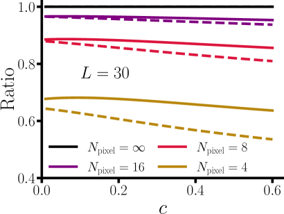
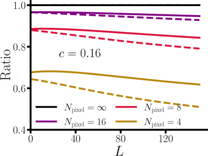
Figure 5: The ratio between the CFI for absorption imaging with finite $N_{\text{pixel}}$ and the $F(c,L)$, i.e., the CFI when $N_{\text{pixel}}=\infty$, in the space of system variables: $c$ and $L$. As the number of pixels in the absorption imaging increases, the ratio is getting closer to 1 (black solid), thus the imaging method results in the precision provided by the $F(c,L)$. For each color, the dashed line is for the periodic boundary condition and the solid line is for the hard-wall boundary condition. When estimating a parameter from the absorption imaging method, the hard-wall geometry gives a larger CFI than that of the ring geometry and also, the former deteriorates much less as $c$ or $L$ grows.

As explained, the absorption imaging is commonly implemented to investigate the characteristics of ultracold atomic systems. This method involves irradiating light to cold atomic gas from above, extracting the optical density captured by the CCD camera below the gas, and converting the optical density to the column density of atoms located above each pixel of the camera. In Sec. III.2, this process has been modeled as dividing the finite one-dimensional space into $N_{\text{pixel}}$ pixels and counting the number of atoms in each pixel bin. We can calculate the CFI for this absorption imaging method and compare it to $F_{p}(c,L)$ or $F_{h}(c,L)$, which corresponds to the case when $N_{\text{pixel}}\rightarrow\infty$. The Fig. 5 shows the convergence of CFI for the absorption imaging as the number of pixels increases. The y-axis represents the ratio between the CFI for the absorption imaging and $F(c,L)$. The $F(c,L)$ is calculated using $N=2$ ground state in the LL model. The left plot is when $L$ is fixed and the right plot is when $c$ is fixed. The solid lines indicate the hard-wall geometry and the dashed lines represent the ring geometry. The CFI for the absorption imaging is higher in the hard-wall geometry than in the ring geometry, while both go to the ideal limit, i.e., $F(c,L)$, as $N_{\text{pixel}}$ increases. When $c$ or $L$ increases, the saturation of the CFI for the absorption imaging to the $F(c,L)$ tends to deteriorate, reflecting the Tonks-Girardeau behavior of gas in the $\gamma\rightarrow\infty$ limit. However, the hard-wall geometry shows less deterioration than the ring geometry in this region.

V Summary and Conclusion

We have investigated the Fisher information of the interaction strength in the LL model by calculating it with respect to the eigenstates of the LL Hamiltonian. First we briefly reviewed the Bethe ansatz solutions of the LL model under two different boundary conditions: periodic and hard-wall boundary conditions. Then we discussed the QFI and the CFI in terms of the wavefunction and the condition for the CFI to saturate the QFI. We numerically calculated the Fisher information of interaction strength using the LL eigenfunctions, i.e., Bethe ansatz, and described its behavior in the space of system variables such as interaction strength and system size. We confirmed the negative effect of interaction on the measurement precision and, in particular, found an optimal value of system size for the estimation of interaction strength and the advantage of the hard-wall geometry over the ring geometry. All of these results were reproduced for varying number of particles and with the LL eigenstates of different energies. For the low-lying excitations, we explained the different aspects of type-I and type-II excited states appearing in the functional profile of Fisher information based on its invariance with respect to some symmetry operations on a set of quantum numbers. Finally, we showed that the CFI supported by the absorption imaging method converges to the wavefunction-based CFI as the pixel size in the model of absorption imaging improves. This demonstrates that the precision achievable by the ideal position measurement on $N$ particles can be attained by elaborating the resolution of absorption imaging.

From the viewpoint of quantum metrology, our analysis is selecting a different metrological framework from the typical protocol, where a Hamiltonian parameter is imprinted by the unitary process on a quantum state, which is initially irrelevant to the parameter to be estimated. Here we rather try to determine the attainable precision of estimating a Hamiltonian parameter using the eigenstates of that Hamiltonian which already contain the information of the target parameter. Within this framework, instead of improving the $N$-scaling of Fisher information, we have focused on its behavior in the parameter space and the precision limit that can be obtained by a realistic measurement, e.g., absorption imaging, which is the representative measurement to explore the ultracold atomic systems. It is expected that these results can be utilized in the technique of adaptive measurement, to enhance the estimation precision of the interaction strength in ultracold bosonic gases.

There have been numerous investigations of the LL model under two extreme limits of the Lieb’s parameter $\gamma$: weakly and strongly interacting regimes, which are defined by $\gamma\rightarrow 0$ and $\gamma\rightarrow\infty$, respectively. However, we confirmed that the optimal value of the resource parameter, i.e., system size, that maximizes the Fisher information of the target parameter, i.e., interaction strength, appears in the intermediate regime: $\gamma\sim O(1)$. Hence the present results for the Fisher information, highlighting the distinguishability of the Bethe ansatz solutions for varying $\gamma$, reveal that the intermediate regime of the LL model is in fact the most intriguing one, as demonstrated by its metrological usefulness.

*

Appendix A Bosonic gas in a box trap

The exact solution for $N$ bosons in a box of length $L$ is summarized here. The system is formulated by $\hat{H}\,\Psi=E\,\Psi$ with the following Hamiltonian and boundary conditions:

$$\hat{H}=-\sum_{j=1}^{N}\frac{\partial^{2}}{\partial x_{j}^{2}}+2\,c\sum_{j<l}\delta(x_{j}-x_{l})\,,$$ (23a)

$$\Psi(x_{1}=0,x_{2},\cdots,x_{N})=\Psi(x_{1},\cdots,x_{N-1},x_{N}=L)=0\,,$$ (23b)

where $c>0$ and $\hbar=2m=1$ for the units. The $\Psi$ is symmetric under the exchange of arbitrary two spatial coordinates, thus it is fully defined in the restricted real space $[0,L]^{N}$ once defined in the domain $D:0\leq x_{1}\leq x_{2}\leq\cdots\leq x_{N}\leq L$.

The (unnormalized) solution for the domain $D$ is given by the Bethe ansatz of the following form [6, 8, 10]:

$$\tilde{\psi}(x_{1},\cdots,x_{N})=\!\!\sum_{\epsilon_{1},\cdots,\epsilon_{N}} \!\sum_{P}\epsilon_{1}\epsilon_{2}\cdots\epsilon_{N}A(\epsilon_{1}k_{P_{1}},\cdots,\epsilon_{N}k_{P_{N}})\,e^{i\sum_{j=1}^{N}\epsilon_{j}k_{P_{j}}x_{j}}\,,$$ (24)

$$A(\epsilon_{1}k_{P_{1}},\cdots,\epsilon_{N}k_{P_{N}})\; =\prod_{j<l}\Big{(}1-\frac{i\,c}{\epsilon_{j}k_{P_{j}}+\epsilon_{l}k_{P_{l}}}\Big{)}\Big{(}1+\frac{i\,c}{\epsilon_{j}k_{P_{j}}-\epsilon_{l}k_{P_{l}}}\Big{)}\,,$$

in which $\epsilon_{j}$ is summed over $\pm 1$ and $P$ runs over all permutations of $[1,2,\cdots,N]$. The sign of $k_{j}$ is absorbed into $\epsilon_{j}$ to make $k_{j}>0$ for all $j$’s and also $k_{1}<k_{2}<\cdots<k_{N}$ is assumed without loss of generality due to the sum over $P$. Now one can find the corresponding energy $E=\sum_{j=1}^{N}k_{j}^{2}$ when $x_{j}\neq x_{j+1}\,(\text{i.e.}\,x_{1}<x_{2}<\cdots<x_{N})$ and the rule of exchanging neighboring arguments of $A$:

$$A(\cdots,\epsilon_{j}k_{j},\epsilon_{l}k_{l},\cdots)=\frac{\epsilon_{j}k_{j}-\epsilon_{l}k_{l}+i\,c}{\epsilon_{j}k_{j}-\epsilon_{l}k_{l}-i\,c}\,A(\cdots,\epsilon_{l}k_{l},\epsilon_{j}k_{j},\cdots)\,,$$ (25)

which is from the continuity of $\Psi$ at $x_{j}=x_{j+1}$: $c\,\Psi|_{x_{j+1}=x_{j}}=[\partial\Psi/\partial x_{j+1}-\partial\Psi/\partial x_{j}]|_{x_{j+1}=x_{j}}$ .

The first condition in (23b), $\Psi(x_{1}=0,x_{2},\cdots,x_{N})=0$, results in the symmetry of $A$ under the sign reverse of its first argument:

$$A(\epsilon_{j}k_{j},\cdots)=A(-\epsilon_{j}k_{j},\cdots)\,,$$ (26)

and the second condition in (23b), $\Psi(x_{1},\cdots,x_{N-1},x_{N}=L)=0$, provides the additional conditions on $k$’s:

$$e^{i\,2k_{j}L}=\frac{A(\cdots,-k_{j})}{A(\cdots,k_{j})}\,,$$ (27)

where “$\cdots$” abbreviates the same arguments between numerator and denominator. Apply (25) to the numerator of right-hand side in (27) iteratively so that $-k_{j}$ can be placed in the first argument. Then its minus sign can be removed due to (26). Again apply (25) to that numerator repeatedly to get the sign-removed $k_{j}$ back to its original position, that is, to the last argument. Finally, one obtains the Bethe equations from (27):

$$e^{i\,2k_{j}L}=\prod_{l\neq j}\frac{k_{j}+k_{l}+i\,c}{k_{j}+k_{l}-i\,c}\,\frac{k_{j}-k_{l}+i\,c}{k_{j}-k_{l}-i\,c}\,.$$ (28)

Applying the logarithm to the both sides of (28) leads to a systems of $N$ real equations

$$Lk_{j}=\pi n_{j}+\sum_{l\neq j}\left[\tan^{-1}\Big{(}\frac{c}{k_{j}-k_{l}}\Big{)}+\tan^{-1}\Big{(}\frac{c}{k_{j}+k_{l}}\Big{)}\right]$$ (29)

with integer $n_{j}$’s satisfying $1\leq n_{1}\leq n_{2}\leq\cdots\leq n_{N}$. A different form of Bethe equations is obtained using $\tan^{-1}(X)=\pm\frac{\pi}{2}-\tan^{-1}(\frac{1}{X})$ when $X\gtrless 0$:

$$Lk_{j}=\pi I_{j}-\sum_{l\neq j}\left[\tan^{-1}\Big{(}\frac{k_{j}-k_{l}}{c}\Big{)}+\tan^{-1}\Big{(}\frac{k_{j}+k_{l}}{c}\Big{)}\right],$$ (30)

where $I_{j}=n_{j}+j-1$. Note that the $n_{j}$ allow duplicate values, but $I_{j}$’s do not. For example, the ground state corresponds to $n_{1}=n_{2}=\cdots n_{N}=1$ or $I_{1}=1,\,I_{2}=2,\,\cdots,\,I_{N}=N$.

The wavefunction (24) is not normalized yet. Gaudin conjectured the norm of the Bethe ansatz in the Lieb-Liniger model under the periodic boundary condition [10] and Korepin proved it [49]. For the current hard-wall boundary condition (23b), we modify Gaudin’s conjecture and suggest the normalized form of (24) as

$$\psi(x_{1},\cdots,x_{N})=2^{-\frac{N}{2}}\big{|}\mathbf{H}(B)\big{|}^{-\frac{1}{2}}\!\!\!\!\sum_{\epsilon_{1},\cdots,\epsilon_{N}}\!\!\sum_{P}\epsilon_{1}\cdots\epsilon_{N}(-)^{P}\!\exp\!\left\{\frac{i}{2}\sum_{j<l}\phi_{P_{j},P_{l}}^{\epsilon_{j},\epsilon_{l}}-\frac{i}{2}\sum_{j<l}\varphi_{P_{j},P_{l}}^{\epsilon_{j},\epsilon_{l}}+i\sum_{j=1}^{N}\epsilon_{j}k_{P_{j}}x_{j}\right\},$$ (31)

where $\phi_{P_{j},P_{l}}^{\epsilon_{j},\epsilon_{l}}:=2\tan^{-1}(\frac{c}{\epsilon_{j}k_{P_{j}}-\epsilon_{l}k_{P_{l}}})$, $\varphi_{P_{j},P_{l}}^{\epsilon_{j},\epsilon_{l}}:=2\tan^{-1}(\frac{c}{\epsilon_{j}k_{P_{j}}+\epsilon_{l}k_{P_{l}}})$, and $(-)^{P}$ is $+$/$-$1 for even/odd permutation($P$). Also, the $|\mathbf{H}(B)|$ is the determinant of the Hessian matrix of $B(k_{1},\cdots,k_{N})$:

$$B(k_{1},\cdots,k_{N}):=\frac{L}{2}\sum_{j=1}^{N}k_{j}^{2}-\pi\sum_{j=1}^{N}I_{j}k_{j}\\ +\frac{1}{2}\sum_{j=1}^{N}\sum_{l\neq j}\Big{[}\int_{0}^{k_{j}-k_{l}}\!\!\!\!dk\tan^{-1}\!\!\big{(}\frac{k}{c}\big{)}+\!\int_{0}^{k_{j}+k_{l}}\!\!\!\!dk\tan^{-1}\!\!\big{(}\frac{k}{c}\big{)}\Big{]}.$$

Then the norm squared of (24) can be explicitly written as

$$\mathcal{N}^{\,2}=2^{N}\prod_{j<l}\Big{[}1+\frac{c^{2}}{(k_{j}-k_{l})^{2}}\Big{]}\Big{[}1+\frac{c^{2}}{(k_{j}+k_{l})^{2}}\Big{]}\,\text{det}\big{[}\mathbf{H}(B)\big{]},$$ (32)

where the entry of the Hessian $\mathbf{H}(B)$ is

$$\big{[}\mathbf{H}(B)\big{]}_{ij}=\delta_{ij}\bigg{[}L\,+\sum_{l\neq i}\Big{[}\frac{c}{(k_{i}-k_{l})^{2}+c^{2}}+\frac{c}{(k_{i}+k_{l})^{2}+c^{2}}\Big{]}\bigg{]}+\,(1-\delta_{ij})\bigg{[}-\frac{c}{(k_{i}-k_{j})^{2}+c^{2}}+\frac{c}{(k_{i}+k_{j})^{2}+c^{2}}\bigg{]}.$$

We take the $\mathcal{N}$ in (32) as the exact norm of (24) without mathematical rigor being used. We checked empirically that (32) fits well with the numerical result of $\int_{0}^{L}dx_{N}\int_{0}^{x_{N}}dx_{N-1}\cdots\int_{0}^{x_{2}}dx_{1}\big{|}\tilde{\psi}(x_{1},\cdots,x_{N})\big{|}^{2}$.

References

- Paredes et al. [2004] B. Paredes, A. Widera, V. Murg, O. Mandel, S. Fölling, I. Cirac, G. V. Shlyapnikov, T. W. Hänsch, and I. Bloch, Tonks–Girardeau gas of ultracold atoms in an optical lattice, Nature 429, 277 (2004).
- Kinoshita et al. [2006] T. Kinoshita, T. Wenger, and D. S. Weiss, A quantum Newton’s cradle, Nature 440, 900 (2006).
- Bethe [1931] H. Bethe, Zur Theorie der Metalle, Zeitschrift für Physik 71, 205 (1931).
- Batchelor [2006] M. Batchelor, Bethe Ansatz, in Encyclopedia of Mathematical Physics, edited by J.-P. Françoise, G. L. Naber, and T. S. Tsun (Academic Press, Oxford, 2006) pp. 253–257.
- Lieb and Liniger [1963] E. H. Lieb and W. Liniger, Exact Analysis of an Interacting Bose Gas. I. The General Solution and the Ground State, Phys. Rev. 130, 1605 (1963).
- Gaudin [1971] M. Gaudin, Boundary Energy of a Bose Gas in One Dimension, Phys. Rev. A 4, 386 (1971).
- Lieb [1963] E. H. Lieb, Exact Analysis of an Interacting Bose Gas. II. The Excitation Spectrum, Phys. Rev. 130, 1616 (1963).
- Batchelor et al. [2005] M. T. Batchelor, X. W. Guan, N. Oelkers, and C. Lee, The 1D interacting Bose gas in a hard wall box, Journal of Physics A: Mathematical and General 38, 7787 (2005).
- Oelkers et al. [2006] N. Oelkers, M. T. Batchelor, M. Bortz, and X.-W. Guan, Bethe ansatz study of one-dimensional Bose and Fermi gases with periodic and hard wall boundary conditions, Journal of Physics A: Mathematical and General 39, 1073 (2006).
- Gaudin [2014] M. Gaudin, The Bethe Wavefunction, edited by J.-S. Caux (Cambridge University Press, 2014).
- Reichert et al. [2019] B. Reichert, G. E. Astrakharchik, A. Petković, and Z. Ristivojevic, Exact Results for the Boundary Energy of One-Dimensional Bosons, Phys. Rev. Lett. 123, 250602 (2019).
- Dunjko et al. [2001] V. Dunjko, V. Lorent, and M. Olshanii, Bosons in Cigar-Shaped Traps: Thomas-Fermi Regime, Tonks-Girardeau Regime, and In Between, Phys. Rev. Lett. 86, 5413 (2001).
- Lang et al. [2017] G. Lang, F. Hekking, and A. Minguzzi, Ground-state energy and excitation spectrum of the Lieb-Liniger model : accurate analytical results and conjectures about the exact solution, SciPost Phys. 3, 003 (2017).
- Minguzzi and Vignolo [2022] A. Minguzzi and P. Vignolo, Strongly interacting trapped one-dimensional quantum gases: Exact solution, AVS Quantum Science 4, 027102 (2022).
- Kulish et al. [1976] P. P. Kulish, S. V. Manakov, and L. D. Faddeev, Comparison of the exact quantum and quasiclassical results for a nonlinear Schrödinger equation, Theoretical and Mathematical Physics 28, 615 (1976).
- Ishikawa and Takayama [1980] M. Ishikawa and H. Takayama, Solitons in a One-Dimensional Bose System with the Repulsive Delta-Function Interaction, Journal of the Physical Society of Japan 49, 1242 (1980).
- Mottelson [1999] B. Mottelson, Yrast Spectra of Weakly Interacting Bose-Einstein Condensates, Phys. Rev. Lett. 83, 2695 (1999).
- Syrwid and Sacha [2015] A. Syrwid and K. Sacha, Lieb-Liniger model: Emergence of dark solitons in the course of measurements of particle positions, Phys. Rev. A 92, 032110 (2015).
- Golletz et al. [2020] W. Golletz, W. Górecki, R. Ołdziejewski, and K. Pawłowski, Dark solitons revealed in Lieb-Liniger eigenstates, Phys. Rev. Research 2, 033368 (2020).
- Syrwid [2021] A. Syrwid, Quantum dark solitons in ultracold one-dimensional Bose and Fermi gases, Journal of Physics B: Atomic, Molecular and Optical Physics 54, 103001 (2021).
- Alon and Cederbaum [2005] O. E. Alon and L. S. Cederbaum, Pathway from Condensation via Fragmentation to Fermionization of Cold Bosonic Systems, Phys. Rev. Lett. 95, 140402 (2005).
- Marchukov and Fischer [2019] O. V. Marchukov and U. R. Fischer, Self-consistent determination of the many-body state of ultracold bosonic atoms in a one-dimensional harmonic trap, Annals of Physics 405, 274 (2019).
- Gwak et al. [2021] Y. Gwak, O. V. Marchukov, and U. R. Fischer, Benchmarking the multiconfigurational Hartree method by the exact wavefunction of two harmonically trapped bosons with contact interaction, Annals of Physics 434, 168592 (2021).
- Wootters [1981] W. K. Wootters, Statistical distance and Hilbert space, Phys. Rev. D 23, 357 (1981).
- Helstrom [1967] C. Helstrom, Minimum mean-squared error of estimates in quantum statistics, Physics Letters A 25, 101 (1967).
- Braunstein and Caves [1994] S. L. Braunstein and C. M. Caves, Statistical distance and the geometry of quantum states, Phys. Rev. Lett. 72, 3439 (1994).
- Paris [2009] M. G. A. Paris, Quantum estimation for quantum technology, International Journal of Quantum Information 07, 125 (2009).
- Wiseman and Milburn [2009] H. M. Wiseman and G. J. Milburn, Quantum Measurement and Control (Cambridge University Press, 2009).
- Giovannetti et al. [2011] V. Giovannetti, S. Lloyd, and L. Maccone, Advances in quantum metrology, Nature Photonics 5, 222 (2011).
- Giovannetti et al. [2006] V. Giovannetti, S. Lloyd, and L. Maccone, Quantum Metrology, Phys. Rev. Lett. 96, 010401 (2006).
- Braunstein [1992] S. L. Braunstein, Quantum limits on precision measurements of phase, Phys. Rev. Lett. 69, 3598 (1992).
- Giovannetti et al. [2004] V. Giovannetti, S. Lloyd, and L. Maccone, Quantum-Enhanced Measurements: Beating the Standard Quantum Limit, Science 306, 1330 (2004).
- Boixo et al. [2007] S. Boixo, S. T. Flammia, C. M. Caves, and J. Geremia, Generalized Limits for Single-Parameter Quantum Estimation, Phys. Rev. Lett. 98, 090401 (2007).
- Boixo et al. [2008a] S. Boixo, A. Datta, S. T. Flammia, A. Shaji, E. Bagan, and C. M. Caves, Quantum-limited metrology with product states, Phys. Rev. A 77, 012317 (2008a).
- Boixo et al. [2008b] S. Boixo, A. Datta, M. J. Davis, S. T. Flammia, A. Shaji, and C. M. Caves, Quantum Metrology: Dynamics versus Entanglement, Phys. Rev. Lett. 101, 040403 (2008b).
- Pang and Jordan [2017] S. Pang and A. N. Jordan, Optimal adaptive control for quantum metrology with time-dependent Hamiltonians, Nature Communications 8, 14695 (2017).
- Barndorff-Nielsen and Gill [2000] O. E. Barndorff-Nielsen and R. D. Gill, Fisher information in quantum statistics, Journal of Physics A: Mathematical and General 33, 4481 (2000).
- Gietka and Chwedeńczuk [2014] K. Gietka and J. Chwedeńczuk, Atom interferometer in a double-well potential, Phys. Rev. A 90, 063601 (2014).
- Wasak et al. [2016] T. Wasak, A. Smerzi, L. Pezzé, and J. Chwedeńczuk, Optimal measurements in phase estimation: simple examples, Quantum Information Processing 15, 2231 (2016).
- Dalton [2007] B. J. Dalton, Two-mode theory of BEC interferometry, Journal of Modern Optics 54, 615 (2007).
- Grond et al. [2011] J. Grond, U. Hohenester, J. Schmiedmayer, and A. Smerzi, Mach-Zehnder interferometry with interacting trapped Bose-Einstein condensates, Phys. Rev. A 84, 023619 (2011).
- Dalton and Ghanbari [2012] B. J. Dalton and S. Ghanbari, Two mode theory of Bose–Einstein condensates: interferometry and the Josephson model, Journal of Modern Optics 59, 287 (2012).
- Javanainen and Chen [2012] J. Javanainen and H. Chen, Optimal measurement precision of a nonlinear interferometer, Phys. Rev. A 85, 063605 (2012).
- Javanainen and Chen [2014] J. Javanainen and H. Chen, Ground state of the double-well condensate for quantum metrology, Phys. Rev. A 89, 033613 (2014).
- Milburn et al. [1997] G. J. Milburn, J. Corney, E. M. Wright, and D. F. Walls, Quantum dynamics of an atomic Bose-Einstein condensate in a double-well potential, Phys. Rev. A 55, 4318 (1997).
- Fraïsse et al. [2019] J. M. E. Fraïsse, J.-G. Baak, and U. R. Fischer, Many-body quantum metrology with scalar bosons in a single potential well, Phys. Rev. A 99, 043618 (2019).
- Anderson et al. [1995] M. H. Anderson, J. R. Ensher, M. R. Matthews, C. E. Wieman, and E. A. Cornell, Observation of Bose-Einstein Condensation in a Dilute Atomic Vapor, Science 269, 198 (1995).
- Andrews et al. [1997] M. R. Andrews, C. G. Townsend, H.-J. Miesner, D. S. Durfee, D. M. Kurn, and W. Ketterle, Observation of Interference Between Two Bose Condensates, Science 275, 637 (1997).
- Korepin [1982] V. E. Korepin, Calculation of norms of Bethe wave functions, Communications in Mathematical Physics 86, 391 (1982).
- Shun-Long [2006] L. Shun-Long, Fisher Information of Wavefunctions: Classical and Quantum, Chinese Physics Letters 23, 3127 (2006).
- Facchi et al. [2010] P. Facchi, R. Kulkarni, V. Man’ko, G. Marmo, E. Sudarshan, and F. Ventriglia, Classical and quantum Fisher information in the geometrical formulation of quantum mechanics, Physics Letters A 374, 4801 (2010).
- Dalfovo et al. [1999] F. Dalfovo, S. Giorgini, L. P. Pitaevskii, and S. Stringari, Theory of Bose-Einstein condensation in trapped gases, Rev. Mod. Phys. 71, 463 (1999).
- Sakmann and Kasevich [2016] K. Sakmann and M. Kasevich, Single-shot simulations of dynamic quantum many-body systems, Nature Physics 12, 451 (2016).
- Lode and Bruder [2017] A. U. J. Lode and C. Bruder, Fragmented Superradiance of a Bose-Einstein Condensate in an Optical Cavity, Phys. Rev. Lett. 118, 013603 (2017).
- Lode et al. [2021] A. U. J. Lode, R. Lin, M. Büttner, L. Papariello, C. Lévêque, R. Chitra, M. C. Tsatsos, D. Jaksch, and P. Molignini, Optimized observable readout from single-shot images of ultracold atoms via machine learning, Phys. Rev. A 104, L041301 (2021).
- Slavnov [1989] N. A. Slavnov, Calculation of scalar products of wave functions and form factors in the framework of the alcebraic Bethe ansatz, Theoretical and Mathematical Physics 79, 502 (1989).
- Chen [2020] H.-H. Chen, Exact overlaps in the Lieb-Liniger model from coordinate Bethe ansatz, Physics Letters B 808, 135631 (2020).
- Sotiriadis [2020] S. Sotiriadis, Non-Equilibrium Steady State of the Lieb-Liniger model: multiple-integral representation of the time evolved many-body wave-function (2020), arXiv:2010.03553 [cond-mat.stat-mech] .
- Zill et al. [2016] J. C. Zill, T. M. Wright, K. V. Kheruntsyan, T. Gasenzer, and M. J. Davis, A coordinate Bethe ansatz approach to the calculation of equilibrium and nonequilibrium correlations of the one-dimensional Bose gas, New Journal of Physics 18, 045010 (2016).
- Pang and Brun [2014] S. Pang and T. A. Brun, Quantum metrology for a general Hamiltonian parameter, Phys. Rev. A 90, 022117 (2014).