What is a combinatorial interpretation?

Abstract.

In this survey we discuss the notion of combinatorial interpretation in the context of Algebraic Combinatorics and related areas. We approach the subject from the Computational Complexity perspective. We review many examples, state a workable definition, discuss many open problems, and present recent results on the subject.

1. Introduction

1.1. What numbers?

Traditionally, Combinatorics  works with numbers. Not with structures, relations between the structures, or connections between the relations — just numbers. These numbers tend to be nonnegative integers, presented in the form of some exact formula or disguised as probability. More importantly, they always count the number of some combinatorial objects.

This approach, with its misleading simplicity, led to a long series of amazing discoveries, too long to be recounted here. It turns out that many interesting combinatorial objects satisfy some formal relationships allowing for their numbers to be analyzed. More impressively, the very same combinatorial objects appear in a number of applications across the sciences.

Now, as structures are added to Combinatorics, the nature of the numbers and our relationship to them changes. They no longer count something explicit or tangible, but rather something ephemeral or esoteric, which can only be understood by invoking further results in the area. Even when you think you are counting something combinatorial, it might take a theorem or a even the whole theory to realize that what you are counting is well defined (see e.g. $\S$4.6).

This is especially true in Algebraic Combinatorics  where the numbers can be, for example, dimensions of invariant spaces, weight multiplicities or Betti numbers. Clearly, all these numbers are nonnegative integers, but as defined they do not count anything per se, at least in the most obvious or natural way.

1.2. Why combinatorial interpretations?

This brings us to the popular belief that one should always look for a combinatorial interpretation (see $\S$15.1). As we see it, there are two reasons for this.

The first reason is clear: when you know what you are counting you have access to a large toolkit already developed in Enumerative Combinatorics and areas further afield. Essentially, the explicit combinatorial objects serve as a common playground where the areas can meet and be understood (see $\S$3.2).

The second, deeper reason, is largely based on the hope is that a combinatorial interpretation would reveal some structures hidden in the algebraic objects they are working with. One can think of combinatorial interpretations as projections — you gather enough projections and hope the whole structure emerges. Consequently, when a combinatorial interpretation is found it is hard to tell if it points to a new structure without further study.

From our perspective, the first reason is terrific and can bring a lot of activity as new combinatorial objects rise to prominence in the areas spurred by applications. Meanwhile, the second reason is unfortunate and indicates that the area does not have a workable definition of a “combinatorial interpretation”. This brings us to the following difficult question.

1.3. What do we mean by a combinatorial interpretation?

Well, this is what this survey is about. The short answer is #P, a computational complexity class which we discuss at length.

But before we proceed, let us make a trivial comment. The first step towards building a theory is admitting the need for a formal definition. Without that, the negative results are impossible to state while the positive results ring hollow and cannot be fully appreciated for the miracle that they are.

According to Popper’s philosophy, a belief needs to be disprovable in order to be scientific [Pop62]. Those who have unquestionable faith in the existence of combinatorial interpretations for all problems they care about, might want to take this lesson to heart.

1.4. There is no there there

We argue that many (all?) long-standing open problems on combinatorial interpretations in Algebraic Combinatorics can be formalized and resolved. We believe that few if any of them will have a solution of the kind that people in the area are looking for.

We aim to give a negative solution to many of the combinatorial interpretation problems using a formal definition we mentioned above. The goal of this paper is to advance this as part of a larger project. Until recently, this seemed overly ambitious and beyond the reach. Hopefully, this survey will leave you more optimistic.

1.5. Why bother?

Given that until recently the notion of “combinatorial interpretation” had been informal, why set on a quixotic journey? Let us frame the question in much broader terms, from the perspective of Computational Combinatorics. There are two fundamental questions we want to address in our study:

$(1)$  How do you prove that given numbers have a  (#P)  combinatorial interpretation?

$(2)$  How do you prove that they do not?

Note that we are not so much interested in finding  an explicit combinatorial interpretation, just proving membership in #P suffices for our purposes. Mostly, we are interested in development of new tools coming both from Combinatorics and Computational Complexity, to resolve the questions above.

In the last few decades, the area of Algebraic Combinatorics did a great job proving relevance and applicability beyond its boundaries. From this point of view, the open problems of finding combinatorial interpretations for numbers such as the Kronecker and Schubert coefficients are key benchmarks. Resolving them in either direction would be an important achievement in the whole Mathematics.

1.6. Why computational complexity?

In other words, is there perhaps a more suitable and easier to understand language in which the problem can be phrased? Perhaps, in terms of integer points in convex polytopes or tilings in the plane? Indeed, both type of combinatorial interpretations do frequently appear in Algebraic Combinatorics and may seem like the natural place to start.

This is both the easiest and the hardest question to answer. The short answer is this: “Computational complexity provides the broadest and the most flexible language”. In fact, prior to converging to #P, we tried a handful of approaches including the ones above. Since the types of “combinatorial interpretations” they gave were rather constrained, we reasoned that negative results would be easier to obtain. Eventually we discarded all such formulations as unconvincing and resigned to the fundamental difficulty and its ever conditional nature of Computational Complexity.

As we see it now, the Computational Complexity is truly foundational for the whole of Mathematics, and allows one to ask questions on the deeper level. While we constrain ourselves with the problem at hand, we refer to [Wig19] for the general picture.

1.7. What to expect from this survey

We assume that the reader is familiar with standard notation, results and ideas in Algebraic Combinatorics, see e.g. [Mac95, Man01, Sag01, Sta99]. After some hesitation, we decided to assume the same about Computational Complexity. We realize this might be unreasonable, and we will provide plenty of examples, but in the 21st century, a research survey is probably not the best place to include a long list of basic definitions.

We do include a quick overview of basic complexity notions (Section 2), but stop short of getting technical. For more details, we recommend [MM11] which is a fun read, [AB09, Pap94b] for standard textbooks on the subject, and [Aar16] for a very readable survey.

1.8. Structure of the paper

In Section 2, we introduce the computational complexity language, followed by Section 3 with many motivating examples. In Section 4, we discuss many examples from Enumerative Combinatorics, the original motivation for combinatorial interpretations (cf. $\S$15.1). In Sections 5 and 6 we survey inequalities in Probabilistic Combinatorics and Order Theory, respectively. The selection of results is somewhat biased and reflects some of our own interests. The goal is prepare the reader for more difficult problems later on.

In Sections 7–10 is the core part of the survey. Here we discuss many functions in Algebraic Combinatorics centered around four subjects: Young tableaux, $S_{n}$ characters, Kronecker and Schubert coefficients. These should be read in order, as they build on top of each other. Sections 9 and 10 have polemical portions at the end, which some readers might disagree with.

The last part of the survey presets our effort to organize the earlier material and make digestible conclusions. In Section 11, we discuss results and bijections in Algebraic Combinatorics centered around the LR rule and the RSK correspondence, which we consider crucially important to the subject. In Section 12, we discuss our recent work [IP22] which develops tools to prove nonexistence of combinatorial interpretations.

In Section 13, we give an annotated list of #P-completeness and #P-hardness results that we omitted earlier to avoid the confusion. These last three sections are independent from each other and should be accessible to experts in the area who skipped earlier section. We conclude with proofs postponed from earlier sections (Section 14), and some final remarks (Section 15).

Notation

Let $\{0,1\}^{n}$ denote the set of sequences of zeros and ones of length $n$, and let $\{0,1\}^{\ast}$ the set of all such sequences of finite length. We use  $\mathbb{N}=\{0,1,2,\ldots\}$  and  $[n]=\{1,\ldots,n\}$. The rest is pretty self-explanatory.

2. Basic Computational Combinatorics

For the purposes of this survey, we will make numerous shortcuts and imprecise statements, largely sacrificing standard definitions and rigor for the sake of clarity and conciseness. We also make our focus quite a bit more narrow than it could be. We beg forgiveness to the experts.

2.1. Combinatorial objects

The notion of a combinatorial object can be viewed as follows. A word is a binary sequence $x\in\{0,1\}^{\ast}$. The size of $x$ is the length $|x|$. In other words, combinatorial objects of size $N$ are encoded by words of length $N$, which in turn correspond to integers  $0\leq a<2^{N}$. For example, a simple graph on $n$ vertices can be viewed as a word of length $\binom{n}{2}$.

Note that we view combinatorial object as more than an abstract concept because the definition includes the presentation. For example, a simple graph on $n$ vertices and $m$ edges can also be presented as a list of edges. The resulting word would be of size $\Theta(m\log n)$. This makes some algorithms faster and other slower, but since $m=O(n^{2})$ the change is at most polynomial for general graphs, so we can ignore it.

On the other hand, the presentation can make a lot of difference for problems in Algebraic Combinatorics. For example, a partition  $\lambda=(4,3,1)\vdash 8$  can be written in binary  $(100,11,1)$  or in unary  $(1111,111,1)$. The binary presentation is more compact, so partitions $\lambda=(\lambda_{1},\ldots,\lambda_{\ell})\vdash n$ with $\ell=O(1)$ have size $O(\log n)$.

On the other hand, for many problems in Algebraic Combinatorics the unary presentation of size $O(n)$ is more appropriate. For example if your problem involves self-conjugate partitions $\lambda=\lambda^{\prime}\vdash n$, we have $\ell(\lambda)\geq\sqrt{n}$, so the binary presentation still requires poly$(n)$ space. Similarly, the unary presentation is more natural when one works with Young diagrams. In summary, every time the problem involves partitions, one should always state whether partitions are given in unary or in binary.

2.2. Classes and functions

The notion of a combinatorial class can be viewed as follows. Define the language as a subset of binary words: $L\subseteq\{0,1\}^{*}$. For example, we can consider the language of words which encode all Hamiltonian graphs. Similarly, we can consider the language of unary encodings of Young tableaux counted by the LR rule, i.e. for every triple of partitions $(\lambda,\mu,\nu)$, there are exactly $c^{\lambda}_{\mu\nu}$ words in the corresponding language.

We write $\overline{L}:=\{0,1\}^{*}\setminus L$ to denote the complement of $L$. There is some ambiguity here depending on the presentation, but in principle $\overline{L}$ can be very large. For example, the complement to the language of Hamiltonian graphs includes both non-Hamiltonian graphs and all words corresponding to non-graphs.

We usually think of a combinatorial function as a function counting combinatorial objects. This can be viewed as special case of the following general definition. Let $f:\{0,1\}^{\ast}\to\mathbb{Z}$ an integer function. Suppose $f(x)=0$ for $x\notin L$, and $f(x)\geq 1$ for $x\in L$. We then say that $f$ is supported on $L$.

For example, the number of Hamiltonian cycles is a function supported on Hamiltonian graphs. Similarly, the LR coefficients is a function  $f:(\lambda,\mu,\nu)\to c^{\lambda}_{\mu\nu}$  supported on triples of partitions where LR coefficients are nonzero.

Note that the language can be defined in a variety of ways: by an explicit function $f$, by a Turing machine, by a formal grammar by an explicit mathematical definition, or by an abstract logical construction. It is important to keep in mind that complexity of $L$ can reflect complexity of its definition, but that does not always hold.

For example, the set of exponents $n$ for which the Fermat Last Theorem (FLT) holds, naturally correspond to a language  $L=\{3,4,5,\ldots\}$. From the mathematical point of view, proving that $n\in L$ becomes increasingly more difficult as $n$ grows, but as a language $L$ is rather simple now that FLT has been proved.

2.3. Decision, search and counting problems

A decision problem is a computational problem defined by the membership in the language. For example, Hamiltonicity is a problem whether the language of Hamiltonian graphs contains a word corresponding to given graph. Similarly, the non-vanishing of LR coefficients problem  $c^{\lambda}_{\mu\nu}>^{?}0$ is a problem whether a triple of partitions $(\lambda,\mu,\nu)$ written in unary is in the language given as a support of the LR coefficients.

A search problems is similar to the decision problem and asks not only to decide $x\in^{?}L$, but also to verify the answer by providing a witness. We formalize this notion below, but for now let us think of this qualitatively rather than quantitatively.

For example, the search problem associated with Hamiltonicity ask to find a Hamiltonian cycle, since that implies that Hamiltonicity by definition. On the other hand, for Non-Hamiltonicity there is no natural witness as nonexistence of a Hamiltonian cycle cannot be easily characterized (for a very good reason, see below). The verifier can simply list all $2^{m}$ subgraphs and supplant a proof that none are a Hamiltonian cycle.

While seemingly harder, in some cases it is possible to use the decision problem as a black box to solve the search problem, by applying it repeatedly for smaller instances. For example, given graph $G$, if $G$ has a Hamiltonian cycle, check if so does $G\smallsetminus e$. Continue removing edges until eventually some edge cannot be removed. Suppose now $G\smallsetminus e$ does not have Hamiltonian cycles. This means that $e$ is an edge in every Hamiltonian cycle in $G$. This reduced the problem to finding a Hamiltonian cycle in $G/e$ obtained from $G$ as contraction by $e$. Proceed in this fashion until the whole Hamiltonian cycle is constructed.

Given a search problem, a counting problem is a problem of computing a function $f$ given by the number of witnesses the verifier can accept. So if $x\notin L$, i.e. the decision problem has a negative answer, the function $f(x):=0$. Otherwise, the function $f(x)\geq 1$ for all $x\in L$, i.e. function $f$ is supported on $L$.

For example, the number of Hamiltonian cycles is a function supported on Hamiltonian graphs which naturally arises that way. Similarly, but less obviously, the LR-coefficients $c^{\lambda}_{\mu\nu}$ is the counting function for the number of LR tableaux.

2.4. Polynomial time problems

Until now we avoided using the words polynomial time, since it makes definitions quantitative and unnecessarily complicates the matter. But we need it from this point.

The first truly important class for us is P. It is a class of languages where the decision problem can be solved in polynomial time. There is a wide variety of problems in this class, for example testing whether a graph is connected or bipartite. More involved graph theoretic problems in P include planarity and having a perfect matching.

Historically, there was a variety of ways to formalize the definition of P, all of which turn out to be equivalent. We will use a Turing machine (TM) mostly out of habit and because it is best known (compared to RAM and other equivalent models of computation). From our point of view, using the colloquial polynomial time algorithm is absolutely fine.

We distinguish class P from the class FP of nonnegative functions which can be computed in polynomial time. To remember the difference, note that the former outputs $0$ or $1$, while the latter can output larger numbers. Simple examples of functions in FP include the number of connected components of a graph, the number of (proper) $2$-colorings, and the number of spanning trees.

2.5. Polynomial time verifier

Now, given a language $L$, the polynomial time verifier is a Turing machine $M$ such that for some fixed polynomials $p,q$ we have:

$\circ$  for all  $x,w\in\{0,1\}^{\ast}$, we have  $M(x,w)\in\{0,1\}$,

$\circ$  for all  $x\in\{0,1\}^{n}$, machine $M$ runs in time $\leq p(n)$,

$\circ$  for all  $x\in L\cap\{0,1\}^{n}$, there exists $w$, s.t.  $|w|\leq q(n)$  and  $M(x,w)=1$,

$\circ$  for all  $x\in\{0,1\}^{n}\smallsetminus L$  and all $w$ s.t.  $|w|\leq q(n)$, we have  $M(x,w)=0$.

In particular, the verifier accepts, i.e. outputs $1$, only if $w$ is a witness for $x\in L$. Note that the witness $w$ have to have polynomial size to avoid the type of witnesses we had seen in the Non-Hamiltonicity problem. This constraint is also necessary for $M$ to work polynomial time, since otherwise it would take exponential time just to read the exhaustive list of subgraphs in this case.

Continuing with our favorite example, in the HamiltonianCycle search problem, the verifier checks if a collection of edges (this is $w$) is a Hamiltonian cycle in graph $G$ (this is $x$ in the notation above). Clearly, this can be done in polynomial time. Similarly, in the LR Tableau search problem, a Young tableau can be verified to be a LR tableau corresponding to a triple $(\lambda,\mu,\nu)$ in polynomial time. This is done by checking all equalities for the shape and the content, and all inequalities involved in the definition: non-increase in rows, strict increase in columns, and balance conditions for the right-to-left reading word.

2.6. Complexity classes

Complexity class NP is the class of decision problems $x\in^{?}L$ for which there exists a polynomial time verifier. Similarly, class coNP is the class of decision problems $x\in^{?}L$, such that there exists a polynomial time verifier for the complementary problem $x\in^{?}\overline{L}$.

For example, Hamiltonicity $\in{\textsf{NP}}$ and Non-Hamiltonicity $\in{\textsf{coNP}}$. Clearly, ${\textsf{P}}\subseteq{\textsf{NP}}\cap{\textsf{coNP}}$. There are several hard decision problems known to be in ${\textsf{NP}}\cap{\textsf{coNP}}$, so it is conjectured that ${\textsf{P}}\neq{\textsf{NP}}\cap{\textsf{coNP}}$. It is also conjectured that ${\textsf{NP}}\neq{\textsf{coNP}}$. It is known that ${\textsf{P}}\neq{\textsf{NP}}$ would not imply either of these two conjectures (see e.g. [Aar16, $\S$2.2.3]).

Next, complexity class #P is the class of counting functions for which there exists a polynomial time verifier. Formally, a function $f:\{0,1\}^{\ast}\to\mathbb{N}$ is in #P if there exists a polynomial time verifier $M$ and polynomial $q:\mathbb{N}\to\mathbb{N}$, such that for all $n\in\mathbb{N}$ we have:

$$f(x)\,=\,\big{|}\big{\{}w\in\{0,1\}^{q(n)}:~{}M(x,w)=1\big{\}}\big{|}\quad\text{for all}\quad x\in\{0,1\}^{n}.$$

Observe that  ${\textsf{FP}}\subseteq{\textsf{\#P}}$. Indeed, for $f\in{\textsf{FP}}$ the witness for $x$ is any integer in  $a\in\big{\{}0,\ldots,f(x)-1\big{\}}$, and the verifier first computes $f(x)$ and then checks if  $a<f(x)$. It is widely assumed that ${\textsf{FP}}\neq{\textsf{\#P}}$. In fact, it is hard to overstate how strong is this assumption.

For example, let $f(G)$ be the number of Hamiltonian cycles in $G$. Then $f\in{\textsf{\#P}}$ since it is counting combinatorial objects which can be verified in polynomial time. Similarly, LR coefficients are given as a function  $(\lambda,\mu,\nu)\to c^{\lambda}_{\mu\nu}$  is also in #P, since it is counting LR-tableaux which can be verified in polynomial time by the argument above. We give many more examples in the next section.

Note that we do not discuss problems that are NP-complete or #P-complete. That’s largely because these notions are largely tangential to this survey. Like with other complexity classes and standard computational complexity notation, we will mention them at will when we need them and hope the reader catches us. Here is a partial list as a mental check for the reader:

$${\textsf{P}}\,\subseteq\,{\textsf{UP}}\,\subseteq\,{\textsf{NP}}\,\subseteq\,\Sigma_{2}^{\textsc{p}}\,\subseteq\,{\textsf{PH}}\,\subseteq\,{\textsf{PSPACE}}\hskip 0.85355pt.$$

We do want to emphasize the distinction of NP-complete and NP-hard classes – the former is contained in NP, while the latter does not. The same with #P-complete and #P-hard classes.

3. Combinatorial interpretation, first steps

3.1. Main definition

We will be brief. Let $f:\{0,1\}^{\ast}\to\mathbb{N}$ be a function. We say that $f$ has a combinatorial interpretation  if

$${f\hskip 1.70709pt\in\hskip 1.70709pt{\textsf{\#P}}}\hskip 0.85355pt.$$

Note that until now, we used the term “combinatorial interpretation” in both its technical and colloquial meaning, which usually coincide but can also differ in several special case. For the rest of the paper, we will use it only in the technical sense, and use quotation marks for the colloquial meaning.

3.2. Basic examples and non-examples

We begin with some motivating examples, mostly following [IP22].

$(1)$   Let  $e:P\to\mathbb{N}$  be the number of linear extensions of $P$, where  $P=(X,\prec)$  is a poset with $n$ elements. Clearly, $e(P)\geq 1$, so we can define a nonnegative function  $e^{\prime}(P):=e(P)-1$. Now observe that  $e^{\prime}\in{\textsf{\#P}}$  simply because finding the lex-smallest linear extension $L$ can be done in polynomial time by a greedy algorithm (see e.g. [CW95]), so  $e^{\prime}(P)$  counts linear extensions of $P$ that are different from $L$.

$(2)$   Let  $G=(V,E)$  be a simple graph with $n=|V|$ vertices and $m=|E|\geq 1$ edges. Let  $c(G)$  be the number of proper $3$-colorings of $G$. Clearly, $c\in{\textsf{\#P}}$. Note that $3^{n}-c(G)$ is also in #P, since verifying that a $3$-coloring is not proper is in P.

Now, taking into account permutations of colors, observe that  $f(G):=c(G)/6$ is an integer valued function. To see that $f(G)\in{\textsf{\#P}}$, note that of the six possible $3$-colorings corresponding to a given $3$-coloring one can easily choose the lex-smallest. In other words the combinatorial interpretation for $f(G)$ is the set of lex-smallest $3$-colorings of $G$.

The key point here is that starting with a $3$-coloring $\chi:V\to\{1,2,3\}$, we can compute in polynomial time the lex-smallest $3$-coloring $\chi^{\prime}$ from the set of 6 recolorings of $\chi$. If $\chi=\chi^{\prime}$, we verify that $\chi$ is a combinatorial interpretation, and discard $\chi$ if otherwise.

$(3)$   Let $G=(V,E)$ be a simple graph with $|V|=n$ vertices and $|E|=m$ edges. Consider the following elegant inequality by Grimmett [Gri76]:

$$(\ast)\qquad\tau(G)\,\leq\,\frac{1}{n}\left(\frac{2\hskip 0.85355ptm}{n-1}\right)^{n-1}$$

for the number $\tau(G)$ of spanning trees in $G$. We can turn this inequality into a nonnegative integer function as follows.

$$f(G)\,:=\,(2\hskip 0.85355ptm)^{n-1}\hskip 1.70709pt-\hskip 1.70709ptn\hskip 0.85355pt(n-1)^{n-1}\hskip 0.85355pt\tau(G)\hskip 0.85355pt.$$

Recall  $\tau(G)\in{\textsf{FP}}$  by the matrix-tree theorem. Then  $f\in{\textsf{FP}}$, and so  $f(G)$  has a combinatorial interpretation according to our definition.

One could argue that a “combinatorial interpretation” should explain why  the inequality $(\ast)$ holds in the first place. In fact, there are several schools of thought on this issue (see a discussion in [Pak18, $\S$4]). We believe that the computational complexity approach is both the least restrictive and the most formal way to address this. Indeed, the combinatorial interpretations we study are depend solely of the functions themselves and not of the difficulty of the proof of the functions being integer or nonnegative.

$(4)$   Let $h(G)$ be the number of Hamiltonian cycles in $G$, and let  $f(G):=\big{(}h(G)-1\big{)}^{2}$. This is our most basic non-example. While we cannot prove unconditionally that $f\notin{\textsf{\#P}}$, we can prove it modulo standard complexity assumptions. Intuitively this is relatively straightforward. Clearly, a poly-time verifier that  $f(H)\neq 0$ is also a poly-time verifier that  $h(G)\neq 1$. A poly-time verifier for  $h(G)\geq 2$  is easy: present two distinct Hamiltonian cycles. On the other hand, a poly-time verifier for  $h(G)=0$  is unlikely since that would imply that ${\textsf{NP}}={\textsf{coNP}}$.

$(5)$   As above, let $h(G)$ be the number of Hamiltonian cycles in $G$. Recall Fermat’s little theorem  states that  $p\hskip 1.70709pt|\hskip 1.70709pta^{p}-a$  for all integers $a$, and prime $p$. Let

$$f(G)\,:=\,\tfrac{1}{p}\bigl{(}h(G)^{p}\hskip 0.85355pt-\hskip 0.85355pth(G)\bigr{)}.$$

It was shown in [IP22, Prop. 7.3.1], that  $f(G)\in{\textsf{\#P}}$. The proof is very short, and a variation on the original proof in [Pet72] (see also [Ges84, Gol56]). We reproduce it here in full.

Proof. Consider sequences  $(a_{1},\ldots,a_{p})$  of integers  $1\leq a_{i}\leq h(G)$  and partition them into orbits under the natural cyclic action of  $\mathbb{Z}/p\mathbb{Z}$. Since $p$ is prime, these orbits have either $1$ or $p$ elements. There are exactly $p$ orbits with one elements, where $a_{1}=\ldots=a_{p}$. The remaining orbits of size $p$ have a total of  $h(G)^{p}-h(G)$  elements. Since $p$ is fixed, the lex-smallest orbit representative can be found in poly-time.  $\square$

$(6)$   Recall the following Smith’s theorem [Tut46]. Let $e=(v,w)$ be an edge in a cubic graph $G$. Then the number $N_{e}(G)$ of Hamiltonian cycles in $G$ containing $e$ is always even. Denote  $f(G,e):=N_{e}(G)/2$. Is  $f\in{\textsf{\#P}}$? We don’t know. This seems unlikely and remains out of reach with existing technology. But let us discuss the context behind this problem.

There are two main proofs of Smith’s theorem. Tutte’s original proof in [Tut46] uses a double counting argument. An algorithmic version of this proof is given by Jensen [Jen12]. The algorithm starts with one Hamiltonian cycle in $G$ containing $e$, and finds another such cycle. Jensen also shows that this algorithm requires an exponential number of steps in the worst case.

The Price–Thomason lollipop algorithm [Pri77, Tho78] gives a more direct combinatorial proof of Smith’s theorem. This algorithm also partitions the set of all Hamiltonian cycles in $G$ containing $e$ into pairs, and is also exponential, see [Cam01, Kra99b].

Conjecture 3.1.

The function  $f(G,e)$  is not in ${{{\sf\#P}}}$.

Note that if either Jessen’s algorithm or the lollipop algorithm were poly-time, this would imply that $f\in{\textsf{\#P}}$. Indeed, by analogy with $(2)$, a poly-time algorithm would allow us to search for Hamiltonian cycles and only count the ones that are lex-smaller than their pairing partner.

3.3. First observations

From the limited number of examples above, here are a few observation. We will develop them further later on.

$(i)$  In combinatorics, nonnegative integer functions don’t come from nowhere. They are either already counting something, e.g. orbits under the action of some group as in $(2)$ and $(5)$, or are byproducts of inequalities as in $(1)$, $(3)$ and $(4)$.

$(ii)$  The inequality in $(i)$ could be rather trivial. For example, we have the trivial inequality  $e(P)\geq 1$ in $(1)$, the AM-GM inequality in $(3)$, and  $x^{2}\geq 0$ in $(4)$. It is the nature of the inequality that determines whether the function is in #P.

$(iii)$  The computational hardness of the functions works only in one direction: if  $f\in{\textsf{FP}}$  then  $f\in{\textsf{\#P}}$, see $(3)$, but if  $f\in{\textsf{\#P}}$-hard then it can go both ways.

$(iv)$  Even for some classical problems like $(6)$, membership in #P can be open.

4. Sequences

The problems in this section come from Enumerative Combinatorics. Although they are not the most interesting questions from the complexity point of view, the problems of finding combinatorial interpretations of integer sequences are much too famous not be addressed. In our notation and problem selection we largely follow [Pak18].

Throughout this section we assume that the input $n$ is in unary. We say that an integer sequence $\{a_{n}\}$ has a combinatorial interpretation if a function $f:n\to a_{n}$ is in #P. Similarly, we say that $\{a_{n}\}$ can be computed in poly-time if $f\in{\textsf{FP}}$. By abuse of notation, we also say that $\{a_{n}\}$ is in #P and FP, respectively.

4.1. Catalan numbers

Recall the Catalan numbers

$$\text{Cat}(n)\ =\ \frac{1}{n+1}\binom{2n}{n}\ =\ \binom{2n}{n}\hskip 1.70709pt-\hskip 1.70709pt\binom{2n}{n-1}\hskip 1.70709pt,$$

see e.g. [OEIS, A000108]. The fractional formula implies that  Cat$(n)>0$, the subtraction formula implies that  Cat$(n)\in\mathbb{Z}$, but a priori it is not immediately obvious that Catalan numbers have any  combinatorial interpretations. Of course, there are over 200 “combinatorial interpretations” of various types given in [Sta15].

Let us show that  $\big{\{}\text{Cat}(n)\big{\}}\in{\textsf{\#P}}$. Recall that  $\text{Cat}(n)$  is equal to the number of ballot sequences, defined as  $0-1$  sequences with $n$ zeros and $n$ ones, s.t. every prefix has at least as many zeroes as ones. This can be checked in time poly$(n)$, which proves that Catalan numbers are in #P.

In fact, just about all “combinatorial interpretations” in [Sta15] can also be used to show that Catalan numbers are in #P, but some are trickier than others. For example, $\text{Cat}(n)$  is the number of $123$-avoiding permutations in $S_{n}$, and one would need to observe that there are  $\binom{n}{3}=O(n^{3})$ possible $3$-subsequences. Thus, verifier checking the $123$-avoidance is in P, as desired.

On the other hand, some “combinatorial interpretations” in [Sta15] are not even counting combinatorial objects, and it can take some effort to give them an equivalent presentation which is in #P. Notably, Exc 195 counts certain regions in $\mathbb{R}^{n}$ in the complement to the Catalan hyperplane arrangement  $\mathcal{C}_{n}$ . This setting raises some interesting computational questions.

To present the regions as a combinatorial objects one can use a collection of signs, one for each hyperplane. Since the arrangement  $\mathcal{C}_{n}$  has $\Theta(n^{2})$ hyperplanes, a trivial consistency check of all $(n+1)$-tuples of hyperplanes would give an exponential time algorithm for testing whether the resulting region is nonempty. This is not good enough for being in #P.

Now, in this specific case of the Catalan arrangement, there is an easy poly-time testing algorithm which uses the simple structures of hyperplanes in  $\mathcal{C}_{n}$  and avoids the redundancy in the exhaustive testing above. This algorithm is the verifier giving the desired combinatorial interpretation.

4.2. Polynomial time computable combinatorial sequences

Note that since $n$ is in unary, the sequence  $\big{\{}\text{Cat}(n)\big{\}}$ is in FP since it can be computed in polynomial time. The same holds for Fibonacci numbers [OEIS, A000045], numbers of involutions [OEIS, A000085], partition numbers [OEIS, A000110], and myriad other sequences which can be computed via recurrence relation.

Formally, we observe in [Pak18, Prop. 2.2] that every D-algebraic sequence  is in FP when the input $n$ is in unary. Thus, in particular, this holds for all algebraic  and P-recursive sequences, see e.g. [Sta99, Ch. 6].

On the other hand, there are sequences which likely cannot be computed in poly$(n)$ time. For example, the number  SAW$(n)$  of self-avoiding walks  of length $n$ in $\mathbb{Z}^{2}$ starting at the origin, is conjectured not to be in FP [Pak18, Conj. 2.14]. Clearly,  $\bigl{\{}\text{SAW}(n)\bigr{\}}\in{\textsf{\#P}}$, so we turn our attention to sequences which are unlikely to be in #P, or are in #P for less obvious reasons.

4.3. Unimodality and log-concavity

Both unimodality and log-concavity properties of combinatorial sequences are heavily studied in the literature, see e.g. [Brä15] (see also [Bre89, Bre94, Sta89] for more dated surveys). Following [Pak19], every time you have an inequality $X\leq Y$, we can convert it into a nonnegative integer $(Y-X)$ and ask if it has a combinatorial interpretation. For combinatorial sequences this is especially notable, and the approach above works well again.

To see explicit examples, recall multi-parameter combinatorial sequences such as binomial coefficients  $\binom{n}{k}$ , Delannoy numbers  $D(i,j)$  [OEIS, A008288], Stirling numbers  of both kinds [OEIS, A008275] and [OEIS, A008277], $q$-binomial coefficients  $\binom{n}{k}_{q}$ (see e.g. [Sta99, $\S$1.7]), etc. All of these satisfy various unimodality and log-concavity properties, e.g.

$$\tbinom{n}{k-1}\tbinom{n}{k+1}\,\leq\,\tbinom{n}{k}^{2}\hskip 1.70709pt,$$

$$D(i,j)\,\leq\,D(i+1,j-1)\quad\text{for all}\quad i<j,\quad\text{and}$$

$$[q^{m-1}]\hskip 0.85355pt\tbinom{n}{k}_{q}\,\leq\,[q^{m}]\hskip 0.85355pt\tbinom{n}{k}_{q}\quad\text{for all}\quad 0<m\leq\tfrac{k(n-k)}{2}\hskip 1.70709pt.$$

We refer to [Sag92, CPP21b] for the first two of these inequalities both of which have a direct injective proof. The last inequality is due to Sylvester [Syl78], see also [PP13, Pro82, Sta89] for modern treatment. Clearly, each of these inequalities has a combinatorial interpretation simply because both sides are in FP. For example,  $\bigl{\{}\tbinom{n}{k}^{2}-\tbinom{n}{k-1}\tbinom{n}{k+1}\bigr{\}}\in{\textsf{FP}}$, etc.

4.4. Partitions

Ramanujan’s congruence  $p(5n-1)\equiv 0\pmod{5}$  has a famous “combinatorial interpretation” by Dyson, who conjectured (among other things) that  $\tfrac{1}{5}\hskip 1.70709ptp(5n-1)$  is equal to the number of partitions $\lambda\vdash(5n-1)$ with rank $\lambda_{1}-\lambda_{1}^{\prime}=0\pmod{5}$, see [Dys44]. This conjecture was proved in [AS54] and later extended in a series of remarkable papers, see [AG88, GKS90, Mah05].

Now, Ramanujan proved many more congruences such as $p(25n-1)\equiv 0\pmod{25}$, see e.g. [Har40, $\S$6.6], but there seem to be no Dyson-style rank statistics in this case. On the other hand, now that the congruence is known, it follows that  $\bigl{\{}\tfrac{1}{25}\hskip 1.70709ptp(25n-1)\bigr{\}}\in{\textsf{FP}}$. This is because

$$\sum_{n=0}^{\infty}\hskip 1.70709ptp(n)\hskip 0.85355ptt^{n}\,=\,\prod_{i=1}^{\infty}\hskip 1.70709pt\frac{1}{1-t^{i}}$$

is D-algebraic, or because $\{p(n)\}$ can be computed in poly$(n)$ time via Euler’s recurrence (among several other ways), see [Pak18, $\S$2.5] and references therein. This implies that  $\bigl{\{}\tfrac{1}{25}\hskip 1.70709ptp(25n-1)\bigr{\}}$  already has  a combinatorial interpretation.

Similarly, the curious inequality  $p_{1\hskip 0.85355pt4}(n)\geq p_{2\hskip 0.85355pt3}(n)$  for the numbers of partitions of $n$ into parts $\pm 1\pmod{5}$ and $\pm 2\pmod{5}$, respectively. Finding an explicit injection proving the inequality was suggested by Ehrenpreis, see [AB89, Kad99]. From the computational complexity point of view, we already have  $\{p_{1\hskip 0.85355pt4}(n)-p_{2\hskip 0.85355pt3}(n)\}\in{\textsf{FP}}$, which shows that the desired injection can be computed in poly-time.

Finally, the log-concavity of the partition function [DP15], implies that the sequence  $\big{\{}p(n)^{2}-p(n-1)\hskip 0.85355ptp(n+1)\,,\,n>25\big{\}}$  is in #P, simply because  $\{p(n)\}\in{\textsf{FP}}$.

4.5. Unlabeled graphs

Let $u_{n}$ be the number of non-isomorphic unlabeled graphs on $n$ vertices, see [OEIS, A000088]. Wilf conjectured in [Wilf82], that $\{u_{n}\}$ cannot be computed in poly$(n)$ time, see also [Pak18, Conj. 1.1]. Does $\{u_{n}\}$ have a combinatorial interpretation? This is not so clear. The difficulty is that we are counting orbits rather than combinatorial objects and there is no obvious way to choose orbit representatives:

Open Problem 4.1.

The sequence  $\{u_{n}\}$  is in  ${{{\sf\#P}}}$.

To understand the context of this problem, consider a closely related sequence. Let $a_{n}$ be the number of nonisomorphic unlabeled plane triangulations on $n$ vertices, see [OEIS, A000109]. In [Pak18, Conj. 1.3], we conjectured that $\{a_{n}\}$ be computed in poly$(n)$ time. This would immediately imply that $\{a_{n}\}$ is in FP and thus in #P. Since the conjecture remains open, we show the latter directly:

Proposition 4.2.

The sequence  $\{a_{n}\}$  is in  ${{{\sf\#P}}}$.

We postpone the proof until $\S$14.1. The idea that the group of automorphisms of triangulations has polynomial size and all automorphism can be computed explicitly via a poly-time algorithm for the isomorphism of planar graphs. We are able to compute the whole orbit and then use symmetry breaking by taking lex-smallest orbit representative.

Conjecture 4.3 ([Pak18, Conj. 1.3]).

The sequence  $\{a_{n}\}$  is in  ${{\sf FP}}$.

We believe that this conjecture can be derived using the tools in [Fusy05, KS18]. Back to the sequence $\{u_{n}\}$. If GraphIsomorphism was known to be in P, one could try to use the symmetry breaking approach in the proof of Proposition 4.2. Babai’s recent quasipolynomial upper bound  $n^{O((\log n)^{c})}$  on graph isomorphism [Bab18], falls short of what we need towards resolving Open Problem 4.1.

Note that plane triangulations are dual to $3$-connected cubic graphs, so the following problem lies in between Proposition 4.2 and Open Problem 4.1.

Conjecture 4.4.

Let  $R_{k}(n)$  be the number of  $k$-regular unlabeled graphs on  $n$  vertices. Then  $\big{\{}R_{k}(n)\big{\}}$  is in  ${{{\sf\#P}}}$, for all  $k\geq 1$.

We are optimistic about this conjecture since for $k$-regular graphs the GraphIsomorphism problem is in P. This was proved by Luks in [Luks82], see also [BL83, SW19].

Finally, there is a curious connection to log-concavity (see $\S$4.3). Denote by  $u_{n}(m)$  the number of nonisomorphic graphs with  $n$  vertices and  $m$  edges. It follows from [PR86] (see also [Vat18]), that  $u_{n}(m)^{2}\geq u_{n}(m-1)\hskip 0.85355ptu_{n}(m+1)$. If  $\{u_{n}(m)\}\in{\textsf{\#P}}$ (see Open Problem 4.1), it would make sese to ask if we also have  $\big{\{}u_{n}(m-1)\hskip 0.85355ptu_{n}(m+1)-u_{n}(m)^{2}\big{\}}\in{\textsf{\#P}}$. Analogous questions can be asked about non-isomorphic planar graphs, plane triangulations, etc.

4.6. Knots

Denote by  $k_{n}$  the number of distinct knots with bridge number at most $n$, see e.g. [OEIS, A086825]. Here the bridge number is a knot invariant defined as the minimal number of bridges required to draw a knot in the plane, see e.g. [Mur96, $\S$4.3].

Open Problem 4.5.

The sequence  $\{k_{n}\}$  is not in  ${{{\sf\#P}}}$.

To underscore combinatorial nature of the problem, note that knot diagrams are a (subset of) planar $4$-regular graphs with signs at the vertices, so $n$ is the bound on the number of vertices. The difficulty starts with the word “distinct” which is formalized as non-isotopic and is also combinatorial in nature: two knots are isotopic if they are connected by a finite sequence of Reidemeister moves. Unfortunately, from computational point of view, the issue with identifying distinct knots is much deeper than with nonisomorphic graphs.

First, note that it is not at all obvious that the isotopy is decidable. Could it be that the number of necessary Reidemeister moves between two isotopic knots with $n$ crossings grows faster than the busy beaver function? The answer turns out to be “No”; the sequence $\{k_{n}\}$ is computable indeed. The best known upper bound on the number of Reidemeister moves is the tower of twos of height $2^{O(n)}$ is given by Coward and Lackenby [CL14].

We conclude with a simpler problem, or at least the one that has been resolved. Denote by  $a_{n}$  the number of knot diagrams on $n$ labeled crossings which are isotopic to the unknot. The fact that $\{a_{n}\}$ is in #P follows from a famous result by Hass, Lagarias and Pippenger [HLP99]. Similarly, denote by  $b_{n}$  the number of knot diagrams on $n$ labeled crossings which are not isotopic to the unknot. The sequence $\{b_{n}\}$ is also in #P by a recent result of Agol, see [Lac17, $\S$3.5].

5. Subgraphs

Discrete Probability is a major source of combinatorial inequalities, most of which can be converted into nonnegative functions. Whether these functions are in #P is then a challenging problem. In this section we concentrate on various counting subgraphs problems.

5.1. Matchings

Let $G=(V,E)$ be a simple graph, and let $p(G,k)$ denote the number of $k$-matchings in a simple graph $G=(V,E)$ defined as the number of $k$-subsets of $E$ of pairwise nonadjacent edges. Clearly, $p(G,k)\in{\textsf{\#P}}$. Following [Pak19], consider a function

$$f(G,k)\,:=\,p(G,k)^{2}\hskip 1.70709pt-\hskip 1.70709ptp(G,k-1)\hskip 1.70709ptp(G,k+1).$$

Famously, Heilmann and Lieb proved that $f(G,k)\geq 0$ [HL72], see also [God93, $\S$6.3] and [MSS15] for more context on this remarkable result. It was observed in [Pak19] that $f\in{\textsf{\#P}}$ follows immediately from Krattenthaler’s injective proof of the Heilmann–Lieb theorem [Kra96].

Define  $q(G)$ denote the number of spanning subgraphs  $H=(V,E^{\prime})$,  $E^{\prime}\subseteq E$, which contain a perfect matching. Observe that the function  $q\in{\textsf{\#P}}$, since testing whether $H$ has perfect matching is in P, see e.g. [LP86, $\S$9.1]. The following subsection shows that this is unlikely for other graph properties.

5.2. Hamiltonian subgraphs

Let $f(G)$ denote the number of Hamiltonian spanning subgraphs of a simple graph $G=(V,E)$. Whether $f\in^{?}{\textsf{\#P}}$ is a difficult question and does not follow directly from the definition since we need a poly-time algorithm to decide Hamiltonicity of $G$.

Note that this is a close call, since there is an algorithm to verify that each $H$ is Hamiltonian by showing a Hamiltonian cycle $C$ in $H$. Thus, one would think that pairs $(H,C)$ give a combinatorial interpretation of $f$, but of course one would need to pick only one such cycle $C$ per $H$. For example, the lex-smallest $C$ would work, but there is no poly-time algorithm to verify that.

Open Problem 5.1.

Function  $f$  is not in  ${{{\sf\#P}}}$.

Even more difficult is the  $\overline{f}(G):=2^{m}-f(G)$  function which counts non-Hamiltonian spanning subgraphs of $G$, since there is no efficient verifier in this case. That makes the following problem a little more approachable, perhaps:

Conjecture 5.2.

Function  $\overline{f}$  is not in  ${{{\sf\#P}}}$.

5.3. Spanning forests

Let $G=(V,E)$ be a simple connected graph with $n=|V|$ vertices, and let $F(G,k)$ denote the number of spanning forests in $G$ with $k$ edges. A special case of the celebrated result by Adiprasito, Huh and Katz [AHK18], proves log-concavity of  $\{F(G,k)\}$:

$$(\star)\qquad F(G,k)^{2}\,\geq\,F(G,k-1)\cdot F(G,k+1)\quad\text{for all}\quad 1\leq k\leq n-2.$$

Following [Pak19], define  $f(G,k):=F(G,k)^{2}-F(G,k-1)\hskip 0.85355ptF(G,k+1)$.

Conjecture 5.3.

Function  $f$  is not in  ${{{\sf\#P}}}$.

We have relatively little evidence in favor of this conjecture other than we tried very hard and failed to show that $f\in{\textsf{\#P}}$. The original proof was significantly strengthened and simplified in [ALOV18, BH20, CP21] (see also [CP22] for a friendly exposition).

5.4. Perfect matchings

Let  $G=(V,E)$  be a $k$-regular bipartite multigraph on $2n$ vertices, and let $\text{{\rm PM}}(G)$ be the number of perfect matchings in $G$. The celebrated van der Waerden Conjecture, now proved (see e.g. [vL82] and [LP86, $\S$8.1]), is equivalent to

$$\text{{\rm PM}}(G)\hskip 1.70709pt\geq\hskip 1.70709pt\frac{k^{n}\hskip 0.85355ptn!}{n^{n}}\hskip 1.70709pt.$$

Let  $f(G):=n^{n}\hskip 0.85355pt\text{{\rm PM}}(G)-k^{n}n!$  The following result is a variation on [IP22, Thm. 7.1.5], and shows that it is unlikely that $f$ has a combinatorial interpretation.

Proposition 5.4.

Assume that edge multiplicities in graph $G$ are given by  ${{{\sf\#P}}}$  functions.
If  $f\in{{{\sf\#P}}}$, then  ${{\sf PH}}=\Sigma_{2}^{\textsc{p}}$.

Proof.

Let  $n=2$,  $V=\{a_{1},a_{2},b_{1},b_{2}\}$, and let $E$ consists of edges $(a_{1},b_{1})$ and $(a_{2},b_{2})$ with multiplicity $x_{1}$, edges $(a_{1},b_{2})$ and $(a_{2},b_{1})$ with multiplicity $x_{2}$. Then $G=(V,E)$ is bipartite and $k$-regular, where  $k=x_{1}+x_{2}$. We have  $\text{{\rm PM}}(G)=x_{1}^{2}+x_{2}^{2}$  and

$$f(G)\hskip 1.70709pt=\hskip 1.70709pt4\hskip 0.85355pt\text{{\rm PM}}(G)\hskip 1.70709pt-\hskip 1.70709pt2\hskip 0.85355ptk^{2}\hskip 1.70709pt=\hskip 1.70709pt4\hskip 0.85355pt(x_{1}^{2}+x_{2}^{2})\hskip 1.70709pt-\hskip 1.70709pt2\hskip 0.85355pt(x_{1}+x_{2})^{2}\hskip 1.70709pt=\hskip 1.70709pt2\hskip 0.85355pt(x_{1}-x_{2})^{2}\hskip 0.85355pt.$$

The result now follows from Corollary 2.3.2 in [IP22]. ∎

Compare this result with Schrijver’s inequality [Schr98]

$$\text{{\rm PM}}(G)\hskip 1.70709pt\geq\hskip 1.70709pt\left(\frac{(k+1)^{k-1}}{k^{k-2}}\right)^{n}\hskip 1.70709pt,$$

for all  $n\geq k\geq 3$. An elementary proof of the $k=3$ case is given in [Voo79]. We challenge the reader to give a direct combinatorial proof of this inequality for any fixed $k>3$.

Finally, let us mention Bregman’s inequality [Bre73] formerly known as Minc’s conjecture (see also [Minc78, $\S$6.2]). In the special case of $k$-regular bipartite simple graphs, the setting of the former Ryser’s conjecture, it gives  $\text{{\rm PM}}(G)^{k}\leq(k!)^{n}$. Since the proof in this case is relatively short, it would be interesting to see if this inequality is in  #P.

5.5. Bunkbed conjecture

Let $G=(V,E)$ be a multigraph. Denote by $G\times K_{2}$ the bunkbed graph obtained as a Cartesian product. Formally, two copies of $G$ are connected by parallel edges as follows: each vertex $v\in V$ corresponds to vertices $v_{0}=(v,0)$ and $v_{1}=(v,1)$ which form an edge $(v_{0},v_{1})$.

For vertices $v,w\in V$, denote by  $B_{0}(v,w)$  and  $B_{1}(v,w)$  the number of spanning subgraphs $H$ of $G\times K_{2}$, such that  $v_{0}\leftrightarrow_{H}w_{0}$  and  $v_{0}\leftrightarrow_{H}w_{1}\hskip 0.85355pt$, respectively. In other words, we are counting subgraphs where $w_{0}$ or $w_{1}$ lie in the same connected component as $v_{0}$.

Conjecture 5.5 (Bunkbed conjecture).

For all  $G=(V,E)$  and all  $v,w\in V$, we have  $B_{0}(v,w)\geq B_{1}(v,w)$.

This conjecture was formulated by Kasteleyn (c. 1985), see [vdBK01, Rem. 5], in the context of percolation, and has become popular in the past two decades, see e.g. [Häg03, Lin11] and most recently [Gri22, HNK21]. The fact that it is notoriously difficult to establish, combinatorially or otherwise, suggests the following:

Conjecture 5.6.

Function  $B_{0}-B_{1}$  is not in  ${{{\sf\#P}}}$.

At first glance this might seem contradictory to the bunkbed conjecture, but notice that it only says that if Conjecture 5.5 holds then it holds for “non-combinatorial reasons”, like the van der Waerden Conjecture. More precisely, Conjecture 5.2 rules out a simple direct injection establishing  $B_{1}\leq B_{0}$. On the other hand, if Conjecture 5.5 is false, then Conjecture 5.2 is trivially true. In other words, Conjecture 5.2 is complementary to the bunkbed conjecture and could be easier to resolve.

Let us note that the bunkbed conjecture is known in a few special cases, such as complete graphs [vHL19] and complete bipartite graphs [Ric22]. It would be interesting to see if the proofs imply that  $B_{0}-B_{1}\in{\textsf{\#P}}$  in all these cases.

5.6. Kleitman’s inequality

Let  $\mathcal{A}$  be a collection of labeled graphs on $[n]=\{1,\ldots,n\}$. We say that $\mathcal{A}$ is hereditary, if for every $G\in\mathcal{A}$ and every spanning subgraph $H$ of $G$, we have $H\in\mathcal{A}$. Examples of hereditary properties include planarity, $3$-colorability, triangle-free, non-connectivity, non-Hamiltonicity, and not containing a perfect matching.

Theorem 5.7 (Kleitman [Kle66]).

Let  $\mathcal{A}$  and  $\mathcal{B}$  be hereditary collections of labeled graphs on $[n]$. Then:

$$|\mathcal{A}|\cdot|\mathcal{B}|\,\leq\,2^{\binom{n}{2}}\cdot|\mathcal{A}\cap\mathcal{B}|\hskip 0.85355pt.$$

This Kleitman’s inequality is easier to understand in probabilistic terms, as having a positive correlation between uniform random graph events:

$$\mathbb{P}[\hskip 0.85355ptG\in\mathcal{A}\hskip 0.85355pt]\hskip 1.70709pt\leq\hskip 1.70709pt\mathbb{P}[\hskip 0.85355ptG\in\mathcal{A}\,|\,G\in\mathcal{B}\hskip 0.85355pt]\hskip 0.85355pt.$$

It is then natural to ask if Kleitman’s inequality is in #P.

Proposition 5.8.

Let  $\mathcal{A}$  and  $\mathcal{B}$  be hereditary collections of labeled graphs on $[n]$, such that the membership problems  $G\in^{?}\mathcal{A}$  and  $G\in^{?}\mathcal{B}$  are in ${{\sf P}}$. Then:

$$2^{\binom{n}{2}}\cdot|\mathcal{A}\cap\mathcal{B}|\hskip 1.70709pt-\hskip 1.70709pt|\mathcal{A}|\cdot|\mathcal{B}|\hskip 1.70709pt\in\hskip 1.70709pt{{{\sf\#P}}}\hskip 0.85355pt.$$

The result follows from Kleitman’s original proof. In this context, let us mention the Ahlswede–Daykin (AD) inequality, which is an advanced generalization of Kleitman’s inequality, see $\S$12.5. Other classical inequalities such as the FKG inequality and the XYZ inequality (see e.g. [AS16, Ch. 6]) are direct consequences of the AD inequality.

In [IP22, Prop. 2.5.1], we prove that assuming the (univariate) Binomial Basis Conjecture (BBC), then AD inequality is not in #P. In fact, our proof shows that already Harris inequality [Har60] is not in #P under BBC. This is in sharp contrast to Proposition 5.7.

5.7. Ising model

In this section, we consider a counting version of the Ising model, see e.g. [Bax82, $\S$1.7] for the introduction.

Let $G=(V,E)$ be a multigraph with $n=|V|$ vertices and $m=|E|$ edges. For a subset $S\subseteq V$, let

$$\alpha(S) :=\,\{(v,w)\in E\,:\,v,w\in S\}\hskip 1.70709pt\cup\hskip 1.70709pt\{(v,w)\in E\,:\,v,w\notin S\}.$$

Define the correlation function

$$\mathrm{Cor}(v,w)\,:=\,\sum_{S\subseteq V\,:\,v,w\hskip 0.85355pt\in\hskip 0.85355pt\alpha(S)}\hskip 1.70709pt4^{|\alpha(S)|}\ -\hskip 1.70709pt\sum_{S\subseteq V\,:\,v,w\hskip 0.85355pt\notin\hskip 0.85355pt\alpha(S)}\hskip 1.70709pt4^{|\alpha(S)|}\,.$$

Note that the statistical sum here is over induced subgraphs rather than the spanning subgraphs in the previous two problems.

Griffiths [Gri67] showed that  $\mathrm{Cor}(v,w)\geq 0$  by an inductive combinatorial argument. When untangled, it can be used to prove the following:

Proposition 5.9.

The correlation function  $\mathrm{Cor}:(G,v,w)\to\mathbb{N}$  is in  ${{{\sf\#P}}}$.

The Griffiths–Kelly–Sherman (GKS) inequality [Gri67, KS68] is a triangle-type inequality for the correlation functions:

$$2^{m}\hskip 1.70709pt\mathrm{Cor}(v,w)\,\sum_{S\subseteq V}\hskip 1.70709pt4^{|\alpha(S)|}\,\geq\,\mathrm{Cor}(v,u)\hskip 1.70709pt\mathrm{Cor}(u,w)\quad\text{for all}\ \ u,\hskip 0.85355ptv,\hskip 0.85355ptw\in V,$$

cf. [GP20, Thm. 3.14] for the planar graphs case.

Conjecture 5.10.

The GKS inequality is not in  ${{{\sf\#P}}}$.

We refer to [GHS70] for an even more curious Griffiths–Hurst–Sherman (GHS) inequality, and to [Ell85] for Statistical Physics context, unified proofs and further references.

6. Linear extensions

As structures go, linear extension of finite posets occupy the middle ground between easy combinatorial objects such as standard Young tableaux or spanning trees, and hard objects such as $3$-colorings of graphs or Hamiltonian cycles.

6.1. Björner–Wachs inequality

Let  $P=(X,\prec)$  be a finite poset. A linear extension of $P$ is a bijection  $\rho:X\to[n]$, such that  $\rho(x)<\rho(y)$  for all  $x\prec y$. Denote by  $\operatorname{\mathcal{E}}(P)$  the set of linear extensions of $P$, and write  $e(P):=|\operatorname{\mathcal{E}}(P)|$.

For each element  $x\in X$, let  $B(x):=\big{\{}y\in X\hskip 1.70709pt:\hskip 1.70709pty\succcurlyeq x\big{\}}$  be the upper order ideal generated by $x$, and let  $b(x):=|B(x)|$. The Björner–Wachs inequality [BW89, Thm 6.3] states that

$$e(P)\,\hskip 1.70709pt\prod_{x\in X}b(x)\ \geq\,n!$$

Proposition 6.1 ([CPP22b, Thm 1.13]).

The Björner–Wachs inequality is in  ${{{\sf\#P}}}$.

The proof in [CPP22b, $\S$3] is essentially the same as the original combinatorial proof by Björner and Wachs. This is in contrast with a probabilistic proof in [CPP22b, $\S$4] via (another) Shepp’s inequality [She80] which in turn uses the FKG inequality. Similarly, this is in contrast with the Hammett–Pittel analytic proof [HP08], and Reiner’s $q$-analogue  based proof given in [CPP22b, $\S$5]. Neither of these three proofs seem to imply the proposition.

6.2. Sidorenko’s inequality

A chain in a poset  $P=(X,\prec)$  is a subset  $\{x_{1},\ldots,x_{\ell}\}\subseteq X$, such that  $x_{1}\prec x_{2}\prec\ldots\prec x_{\ell}\hskip 0.85355pt.$ Denote by  $\mathcal{C}(P)$  the set of chains in $P$.

Suppose  $P=(X,\prec)$  and  $Q=(X,\prec^{\prime})$  be two posets on the same set with  $|X|=n$  elements, such that  $\bigl{|}C\cap C^{\prime}\bigr{|}\leq 1$  for all  $C\in\mathcal{C}(P)$  and  $C^{\prime}\in\mathcal{C}(Q)$. Sidorenko’s inequality states that   $e(P)\hskip 0.85355pte(Q)\geq\hskip 1.70709ptn!$  [Sid91].

Proposition 6.2 ([CPP22b, Thm 1.15] and [GG20b, $\S$3]).

Sidorenko’s inequality is in  ${{{\sf\#P}}}$.

Natural examples of posets  $(P,Q)$  as above, are the permutation posets  $\bigl{(}P_{\sigma},P_{\overline{\sigma}}\bigr{)}$, where  $P_{\sigma}=([n],\prec)$  is defined as  $i\prec j$  if and only if  $i<j$  and  $\sigma(i)<\sigma(j)$  for all  $i,j\in[n]$, and  $\overline{\sigma}:=\bigl{(}\sigma(n),\ldots,\sigma(1)\bigr{)}$. In this case  $P_{\sigma}$  is a $2$-dimensional poset, and  $P_{\overline{\sigma}}$  is its plane dual.

The original proof by Sidorenko was based on combinatorial optimization. Other proofs include and earlier direct surjection by Gaetz and Gao [GG20a], and the geometric proof by Bollobás, Brightwell and Sidorenko [BBS99], via Stanley’s theorem on poset polytopes  [Sta86] and Saint-Raymond’s proof of Mahler’s conjecture for convex corners [StR81]. Neither of these three proofs imply the proposition, at least not directly.

6.3. Stanley’s inequality

Let  $P=(X,\prec)$  be a finite poset. For an element  $x\in X$  and integer  $k\in[n]$, denote by  $\textrm{N}(k)=\textrm{N}(P,x,k)$  the number of linear extensions  $\rho\in\operatorname{\mathcal{E}}(P)$, such that  $\rho(x)=k$. Stanley’s inequality [Sta81, Thm 3.1] states that:

$$\textrm{N}(k)^{2}\,\hskip 1.70709pt\geq\,\hskip 1.70709pt\textrm{N}(k-1)\,\hskip 1.70709pt\textrm{N}(k+1)\quad\text{for all}\ \ 1<k<n\hskip 0.85355pt.$$

Conjecture 6.3.

Stanley’s inequality is not in  ${{{\sf\#P}}}$.

In the past few years, we made a considerable effort trying to resolve this problem. The original proof in [Sta81] is an easy but ingenuous reduction from the Alexandrov–Fenchel inequality, that was used previously to prove the van def Waerden conjecture (see $\S$5.4). Since poset polytopes are rather specialized, initially we hoped that Stanley’s inequality is in #P. Another positive evidence is the recent effective characterization of the equality conditions in Stanley’s inequality, by Shenfeld and van Handel [SvH20]. In our terminology, they showed that the vanishing problem  $\big{\{}\textrm{N}(k)^{2}=^{?}\textrm{N}(k-1)\hskip 1.70709pt\textrm{N}(k+1)\big{\}}$  can be decided in poly-time.

With Chan [CP21], we develop a new combinatorial atlas technology (see also [CP22]), which gave a purely linear algebraic proof of Stanley’s inequality and its generalization to weighted linear extensions (see also [CP22+]). This also allowed us to give a new proof of the equality conditions. Unfortunately, the limit argument in our proof does not allow to give a #P description (see [CP21, $\S$17.17]). Separately, with Chan and Panova, we employed several combinatorial approaches in [CPP21a, CPP22a] to posets of width two, and an algebraic approach in [CPP22b, $\S$7 and $\S$9.11]. Unfortunately, Conjecture 6.3 remains elusive.

6.4. XYZ inequality

Let  $P=(X,\prec)$  be a finite poset, and let  $x,y,z\in X$  be incomparable elements. Let  $P_{xy}:=P\cup\{x\prec y\}$,  $P_{xz}:=P\cup\{x\prec z\}$  and  $P_{xyz}:=P\cup\{x\prec y,x\prec z\}$. Shepp’s classic XYZ inequality [She82], states that

$$e(P\bigr{)}\,e(P_{xyz})\ \geq\ e(P_{xy}\bigr{)}\,e(P_{xz}).$$

As with other correlation inequalities, the XYZ inequality is easier to understand in terms of uniform random linear extensions  $\rho\in\operatorname{\mathcal{E}}(P)$:

$$\mathbb{P}[\hskip 0.85355pt\rho(x)<\rho(y)\,|\,\rho(x)<\rho(z)\hskip 0.85355pt]\,\geq\,\mathbb{P}[\hskip 0.85355pt\rho(x)<\rho(y)\hskip 0.85355pt]\hskip 0.85355pt.$$

Conjecture 6.4.

The XYZ inequality is not in  ${{{\sf\#P}}}$.

The original proof (see also [AS16, $\S$6.4]), uses the FKG inequality, which, like the AD inequality, is not in #P in full generality. A double counting argument proving the XYZ inequality is given in [BT02]. Unfortunately, it does not prove that the inequality is in #P, both because of the double counting argument and the use of BipartiteUnbalance problem, see [IP22, $\S$9.2]. This makes the conjecture especially interesting.

7. Young tableaux

We adopt the standard and largely self-explanatory notation from Algebraic Combinatorics. We refer to [Sag92, Sta99] for both notation and the background. Unless stated otherwise, we use unary encoding for all partition and integer parameters throughout this section. For convenience, we are using notation  $f\leq_{\#}g$  to mean that  $(g-f)\in{\textsf{\#P}}$.

7.1. Standard Young tableaux

Let  $f^{\lambda}=|\operatorname{{\rm SYT}}(\lambda)|$  be the number of standard Young tableaux of shape $\lambda\vdash n$. Recall the hook-length formula:

(HLF) $$f^{\lambda}\,=\,n!\,\prod_{(i,j)\in\lambda}\,\frac{1}{h_{\lambda}(i,j)}\,,$$

where  $h_{\lambda}(i,j)=\lambda_{i}+\lambda^{\prime}_{j}-i-j+1$  is the hook-length in $\lambda$. This implies that  $f^{\lambda}\in{\textsf{FP}}$. Consequently, we have that  $n!/f^{\lambda}\in{\textsf{FP}}$  and  $(f^{\lambda})^{2}\leq_{\#}n!$

Similarly, let  $f^{\lambda/\mu}=|\operatorname{{\rm SYT}}(\lambda/\mu)|$  the number of standard Young tableaux of skew shape $\lambda/\mu$, where $|\lambda/\mu|=n$. Recall the Aitken–Feit determinant formula:

(AFDF) $$f^{\lambda/\mu}\,=\,n!\hskip 1.70709pt\det\left(\frac{1}{(\lambda_{i}-\mu_{j}-i+j)!}\right)_{i,j=1}^{\ell(\lambda)}\,.$$

which proves that  $f^{\lambda}\in{\textsf{FP}}$. Consequently, we have that  $f^{\lambda/\mu}\leq_{\#}n!$

Now, it follows from the Naruse hook-length formula (NHLF) that

($$\otimes f^{\lambda/\mu}\,\prod_{(i,j)\in\lambda/\mu}h_{\lambda}(i,j)\ \geq\ n!\,,$$)

see [MPP18b]. Note that this is a much sharper bound than the one given by the Björner–Wachs inequality (see $\S$6.1).

With Morales and Panova, we gave several proofs of the NHLF and its generalizations, both algebraic and combinatorial [MPP17, MPP18a]. A recursive proof is given by Konvalinka [Kon20]. Finding a direct combinatorial proof which allows efficient sampling from $\operatorname{{\rm SYT}}(\lambda/\mu)$, perhaps generalizing the NPS bijection or the GNW hook walk, remains an important open problem, see e.g. [H+21, $\S$5.6].

Conjecture 7.1.

Inequality ($\otimes$ ‣ 7.1) is in ${{{\sf\#P}}}$.

Remark 7.2.

Even the simplest special cases of $(\otimes)$ are hard to establish directly. For example, rotate diagram $\lambda$ by 180^∘ and denote by $\lambda^{\ast}$ be the resulting skew shape. Let  $h_{\lambda}^{\ast}(i,j):=i+j-1$  be the hook-lengths in $\lambda^{\ast}$. Inequality $(\otimes)$ in this case follows from

$$(\otimes\otimes)\qquad\prod_{(i,j)\in\lambda^{\ast}}h_{(a^{b})}(i,j)\ =\ \prod_{(i,j)\in\lambda}h^{\ast}_{\lambda}(i,j)\ \geq\ \prod_{(i,j)\in\lambda}h_{\lambda}(i,j)\,,$$

where  $a=\lambda_{1}$  and  $b=\ell(\lambda)$, see [MPP18b, Prop. 12.1]. A direct combinatorial proof of $(\otimes\otimes)$ is given in [PPS20]. This proof uses Karamata’s inequality  that is not in #P in full generality, see [IP22, $\S$7.5].

7.2. Semistandard Young tableaux

Let  $K_{\lambda\hskip 0.85355pt\mu}=|\operatorname{SSYT}(\lambda,\mu)|$  be the Kostka numbers, where  $\lambda,\mu\vdash n$. The inequality  $K_{\lambda\mu}\leq_{\#}K_{\lambda\hskip 0.85355pt1^{n}}=f^{\lambda}$  is easy to show directly. Much more interesting is the following generalization.

Let  $\textbf{{a}}=(a_{1},\ldots,a_{\ell})$  and  $\textbf{{b}}=(b_{1},\ldots,b_{\ell})$  be two weakly decreasing vectors. We say that a majorizes b, write  $\textbf{{a}}\trianglerighteq\textbf{{b}}$, if  $a_{1}+\ldots+a_{i}\geq b_{1}+\ldots+b_{i}$  for all $1\leq i<\ell$, and  $a_{1}+\ldots+a_{\ell}=b_{1}+\ldots+b_{\ell}$ . Recall that  $K_{\lambda\mu}\leq K_{\lambda\nu}$  for all  $\mu\trianglerighteq\nu$.

Proposition 7.3.

$K_{\lambda\mu}\leq_{\#}K_{\lambda\nu}$  for all  $\mu\trianglerighteq\nu$.

Although not stated in this language, the proof follows easily from the combinatorial proof in [Whi80]. Here we are using the following trivial observation: if  $f_{1},\ldots,f_{k}\in{\textsf{\#P}}$  for $k=$ poly$(n)$, then  $f_{1}+\ldots+f_{k}\in{\textsf{\#P}}$.

Finally, let  $\lambda,\alpha,\beta,\gamma\vdash n$  be such that  $\alpha\trianglerighteq\beta\trianglerighteq\gamma$  and  $\alpha+\gamma=2\hskip 0.85355pt\beta$. Kostka numbers then satisfy log-concavity property given by the HMMS inequality:  $K_{\lambda\beta}^{2}\geq K_{\lambda\alpha}K_{\lambda\gamma}$  [H+22, Thm 2].

Open Problem 7.4.

The HMMS inequality is not in  ${{{\sf\#P}}}$.

The original proof of the HMMS inequality is based on the Lorentzian property of Schur polynomials. Solving the open problem would give an early indication in favor of Conjecture 5.3, since the log-concavity of forest numbers  $\{F(G,k)\}$  is proved in [BH20] based on the same general approach.

Remark 7.5.

The Dominance order “$\triangleright$” is motivated by a technical part in the proof of the Young symmetrizer  construction, see e.g. [Weyl39, $\S$IV.2] and [Sag01, $\S$2.4], and reflects the inherent planarity of Young diagrams. The algebraic proof of Proposition 7.3 given in [LV73] is based on iterative calculation. We note that [Ver06] emphasizes the importance of identity

$$(\vartriangle)\qquad 1\uparrow^{S_{n}}_{S_{\mu_{1}}\times S_{\mu_{2}}\times\hskip 1.70709pt\cdots}\,\bigcap\ \text{\rm sign}\uparrow^{S_{n}}_{S_{\mu_{1}}\times S_{\mu_{2}}\times\hskip 1.70709pt\cdots}\hskip 1.70709pt=\hskip 1.70709pt\SS^{\mu}$$

(see also [May75]). This is a curious byproduct of the dominance order and its reverse.

7.3. Contingency tables

Let  $\mathcal{T}(\lambda,\mu)$  be the set of contingency tables, defined as nonnegative integer matrices with rows sums $\lambda$ and column sums $\mu$. Denote by  ${\text{\rm T}}(\lambda,\mu):=|\mathcal{T}(\lambda,\mu)|$  the number of such tables. Note that  $K_{\lambda,\mu}\leq_{\#}{\text{\rm T}}(\lambda,\mu)$, where the injection sends  $A\in\operatorname{SSYT}(\lambda,\mu)$  into a matrix  $(m_{ij})\in\mathcal{T}(\lambda,\mu)$, where  $m_{ij}$  is the number of letters $j$ in $i$-th row of $A$.

Barvinok’s inequality [Bar07], states that  ${\text{\rm T}}(\lambda,\mu)\leq{\text{\rm T}}(\nu,\tau)$  for all  $\lambda\trianglerighteq\nu$  and  $\mu\trianglerighteq\tau$.

Proposition 7.6.

Barvinok’s inequality is in  ${{{\sf\#P}}}$.

There are two natural proofs of Proposition 7.6. First, following the original proof in [Bar07, p. 111], one can use the  RSK correspondence, which is poly-time by definition. This gives  ${\text{\rm T}}(\lambda,\mu)=\sum_{\pi}K_{\pi\lambda}K_{\pi\mu}$  and then use Proposition 7.3. We then need to use the inverse RSK correspondence, which is also poly-time. A more direct (still rather involved) approach is outlined in [Pak19].

Remark 7.7.

We note in passing that the log-concavity property for contingency tables remains open. Formally, let  $\lambda,\alpha,\beta,\gamma\vdash n$  be as in the HMMS inequality (see $\S$7.2). Barvinok asks if  ${\text{\rm T}}(\lambda,\beta)^{2}\geq^{?}{\text{\rm T}}(\lambda,\alpha)\hskip 1.70709pt{\text{\rm T}}(\lambda,\gamma)$, see [Bar07, p. 110].

7.4. Littlewood–Richardson coefficients

Let  $c^{\lambda}_{\mu\nu}$  be the Littlewood–Richardson (LR) coefficients, where  $\lambda\vdash n$,  $\mu\vdash k$  and  $\nu\vdash n-k$. Standard combinatorial interpretations for LR coefficients imply:

$$c^{\lambda}_{\mu\hskip 0.85355pt\nu}\hskip 0.85355ptf^{\mu}\hskip 0.85355ptf^{\nu}\,\leq_{\#}\,f^{\lambda}\quad\text{and}\quad c^{\lambda}_{\mu\hskip 0.85355pt\nu}\hskip 0.85355ptf^{\lambda}\,\leq_{\#}\,\tbinom{n}{k}\hskip 0.85355ptf^{\mu}\hskip 0.85355ptf^{\nu}\hskip 1.70709pt.$$

We refer to [Ker84, Whi81, Zel81] for the motivational explanation on how to derive these inequalities from the RSK correspondence or via the jeu-de-taquin correspondence. Taking their product gives  $(c^{\lambda}_{\mu\hskip 0.85355pt\nu})^{2}\leq\binom{n}{k}$, as was recently observed in [PPY19, $\S$4.1]. We call this the PPY inequality.

Open Problem 7.8.

The PPY inequality is not in $\hskip 0.85355pt{{{\sf\#P}}}$.

As we discussed earlier, the problem could be resolved either by a direct injection proving the PPY inequality, or by giving an explicit combinatorial interpretation for  $\binom{n}{k}-(c^{\lambda}_{\mu\hskip 0.85355pt\nu})^{2}$.

The remarkable Lam–Postnikov–Pylyavskyy inequality [LPP07] states that:

(LPP) $$c^{\lambda}_{\mu\hskip 0.85355pt\nu}\hskip 1.70709pt\leq\hskip 1.70709ptc^{\lambda}_{\mu\vee\nu\hskip 1.70709pt\mu\wedge\nu}\,,$$

where  $\mu\vee\nu$  and  $\mu\wedge\nu$  denote the union and the intersection of Young diagrams. The original proof is heavily algebraic and does not seem to give a clue on how this can be proved injectively, see [BBR06] for some special cases.

Open Problem 7.9.

The LPP inequality is not in $\hskip 0.85355pt{{{\sf\#P}}}$.

Note a closely related Björner’s inequality:

$$\tbinom{n}{m}\hskip 0.85355ptf^{\mu}\hskip 0.85355ptf^{\nu}\,\leq\,\tbinom{n}{r}\hskip 0.85355ptf^{\mu\vee\nu}\hskip 0.85355ptf^{\mu\wedge\nu},$$

where  $|\mu|=m$,  $|\mu|+|\nu|=n$  and  $|\mu\wedge\nu|=r$  [Bjö11, $\S$6]. It follows by summing over all $\lambda\vdash n$, of (LPP) multiplied by $f^{\lambda}$. Of course, Björner’s inequality is in FP and follows from the HLF.

7.5. Inverse Kostka numbers

Denote by  $\textbf{{K}}=\big{(}K_{\lambda\mu}\big{)}$  the Kostka matrix. Ordering all partitions w.r.t. the size $n=|\lambda|=|\mu|$ and the majorization order  “$\triangleright$”  and using  $K_{\lambda\lambda}=1$, we conclude that the matrix is upper triangular and thus has an integer inverse. Denote by  $\textbf{{K}}^{-1}=\big{(}K^{-1}_{\lambda\mu}\big{)}$  the inverse Kostka matrix, and by  $K^{-1}_{\lambda\mu}$  the inverse Kostka numbers.

Eğecioğlu and Remmel [ER90] showed that  $K^{-1}_{\lambda\mu}$  has a signed combinatorial interpretation as a sum over certain rim-hook tableaux (RHT) of shape $\lambda$ and weight $\mu$. It follows from the construction that  $K^{-1}$  is in  ${\textsf{GapP}}={\textsf{\#P}}-{\textsf{\#P}}$. Direct involutions proving validity  $\textbf{{K}}\cdot\textbf{{K}}^{-1}=\textbf{{K}}^{-1}\cdot\textbf{{K}}=I$  were given in [ER90, LM06]. Other signed combinatorial interpretations are given in [Duan03, PR17].

Conjecture 7.10.

The function  $|K^{-1}_{\lambda\mu}|$  is not in $\hskip 0.85355pt{{{\sf\#P}}}$.

In other words, the conjecture claims that the absolute value of the inverse Kostka numbers does not have a combinatorial interpretation. Thus, a signed sum over combinatorial objects is the best one can have. Further motivation behind the conjecture will become clear in the next section.

8. Characters

In this section we discuss complexity problems related to $S_{n}$ characters. As before, $n$ and all partitions are given in unary.

8.1. The values

Let  $\chi^{\lambda}(\mu)$  denote the character value of the irreducible $S_{n}$ module  $\SS^{\lambda}$  on the conjugacy class  $[\mu]$, where  $\lambda,\mu\vdash n$. The Murnaghan–Nakayama (MN) rule, see e.g. [Sag92, $\S$4.10] and [Sta99, $\S$7.17], gives a signed combinatorial interpretation for  $\chi^{\lambda}(\mu)$  as a sum of signs over rim-hook tableaux  $\operatorname{{\rm RHT}}(\lambda,\mu)$  of shape $\lambda$ and weight $\mu$. Similar to the inverse Kostka numbers, it follows from the construction that function  $\chi:(\lambda,\mu)\to\mathbb{Z}$  is in  ${\textsf{GapP}}={\textsf{\#P}}-{\textsf{\#P}}$.

Does there exist a combinatorial interpretation of the character square  $\bigl{(}\chi^{\lambda}(\mu)\bigr{)}^{2}$? This is an interesting question, and the answer is even more interesting. On the one hand, the answer is yes when  $\mu=(k^{n/k})$  is a rectangle. In this case, all rim-hook tableaux in  $\operatorname{{\rm RHT}}(\lambda,\mu)$  have the same sign, see e.g. [JK81, $\S$2.7] and [SW85], so  $\big{(}\chi^{\lambda}(\mu)\big{)}^{2}=|\operatorname{{\rm RHT}}(\lambda,\mu)|^{2}$  has a combinatorial interpretation as the number of ordered pairs of rim-hook tableaux.

On the other hand, in full generality we have:

Theorem 8.1 ([IPP22]).

If  $(\chi)^{2}\in{{{\sf\#P}}}$, then  ${{\sf coNP}}={{\sf C_{=}P}}$  and  ${{\sf PH}}=\Sigma_{2}^{\textsc{p}}$ .

In other words, it is very unlikely that character square has a combinatorial interpretation, assuming th polynomial hierarchy does not collapse to the second level.

Remark 8.2.

Following [IPP22], one way to understand the implications of the theorem is to compare two identities:

$$n!\,=\,\sum_{\lambda\vdash n}\,\big{(}\chi^{\lambda}(1)\big{)}^{2}\quad\text{and}\quad n!\,=\,\sum_{\pi\in S_{n}}\big{(}\chi^{\lambda}(\pi)\big{)}^{2}\,,\ \ \hskip 1.70709pt\text{for all \ $\lambda\vdash n$.}$$

The former is the Burnside identity  since  $\chi^{\lambda}(1)=f^{\lambda}$, and follows from the RSK correspondence. The latter is the character orthogonality formula, and the theorem explains why there is no natural analogue of the RSK correspondence in this case. Simply put, the terms on the right are not actually counting any combinatorial objects.

8.2. Row and column sums

In [Sta00, $\S$3], Stanley defines

$$a_{\lambda}\hskip 1.70709pt:=\hskip 1.70709pt\sum_{\mu\vdash n}\hskip 1.70709pt\chi^{\lambda}(\mu)\quad\text{and}\quad b_{\lambda}\hskip 1.70709pt:=\hskip 1.70709pt\sum_{\mu\vdash n}\hskip 1.70709pt\chi^{\mu}(\lambda)\hskip 1.70709pt,\quad\text{where \ $\lambda\vdash n$.}$$

which he calls row sums and column sums in the character table, respectively. It is known that  $b_{\lambda}=\bigl{|}\{\omega\in S_{n}\,:\,\omega^{2}=\sigma\}\bigr{|}$, where  $\sigma\in[\lambda]$  is a fixed permutation of type $\lambda$, see e.g. [Sta99, Exc 7.69] and [Mac95, Ex. 11, p. 120]. Thus, the column sums are in #P. One can ask a similar question about the row sums.

First, we note that  $a_{\lambda}\geq 0$  for all $\lambda$. This follows from the fact that  $a_{\lambda}=\langle\rho_{n},\chi^{\lambda}\rangle$, where  $\rho_{n}$  is the character of the conjugation representation, see e.g. [Sta99, Exc 7.71].

Conjecture 8.3 (cf. Problem 12 in [Sta00]).

Row sums  $\{a_{\lambda}\}$  are not in $\hskip 0.85355pt{{{\sf\#P}}}$.

In fact, there are very few cases when a combinatorial interpretation of  $a_{\lambda}$  is known. For example,  $a_{(n)}=p(n)$  and  $a_{(1^{n})}=|\{\lambda\vdash n\hskip 1.70709pt:\hskip 1.70709pt\lambda=\lambda^{\prime}\}|$, see [BE16, Prop. 1]. Proving the conjecture would represent a major advance in the area, as we explain below.

Remark 8.4.

The total sum of the entries in the character tables of $S_{n}$ is a sequence of interest in its own right, see [OEIS, A082733]. So is the determinant of the character table, see [Jam78, Cor. 6.5] and [OEIS, A007870], and even the permanent [SS84].

8.3. Refinements

Denote by  $\rho^{\mu}[\sigma]:=|\{\omega\in[\mu]\hskip 1.70709pt:\hskip 1.70709pt\omega\sigma=\sigma\omega\}|$, where  $[\mu]\subset S_{n}$ is the conjugacy class of permutations of type $\mu\vdash n$. In other words,  $\rho^{\mu}$  is the character of the conjugation action on the conjugacy class $[\mu]$. From above, we have  $\rho_{n}=\sum_{\mu\vdash n}\rho^{\mu}$. Define refined row sums  $a_{\lambda\mu}:=\langle\rho^{\mu},\chi^{\lambda}\rangle\in\mathbb{N}$, and note that  $a_{\lambda}=\sum_{\mu\vdash n}a_{\lambda\mu}$ .

Conjecture 8.5.

Refined row sums  $\{a_{\lambda\mu}\}$  are not in $\hskip 0.85355pt{{{\sf\#P}}}$.

Clearly, the proof of Conjecture 8.3 implies the same for Conjecture 8.5. We warn the reader that it does not follow from definition that  $\{a_{\lambda\mu}\}\in{\textsf{GapP}}$. Indeed, the definition states

$$a_{\lambda\mu}\,:=\,\langle\rho^{\mu},\chi^{\lambda}\rangle\,=\,\frac{1}{n!}\hskip 1.70709pt\sum_{\omega\in S_{n}}\hskip 1.70709pt\rho^{\mu}[\sigma]\hskip 1.70709pt\chi^{\lambda}[\omega]\hskip 1.70709pt.$$

Even though the terms on the RHS are in #P, there is no obvious way to divide the sum by $n!$ The claim is true nonetheless, as we explain later in this section.

Towards the open problem, it was proved by Kraśkiewicz and Weyman [KW01] (see also [Sta99, Exc 7.88b] and [RW20, $\S$3]), that

(KW) $$a_{\lambda\hskip 0.85355pt(n)}\,=\,\big{|}\bigl{\{}A\in\operatorname{{\rm SYT}}(\lambda)\ :\ \mathrm{maj}(A)=0\mod n\bigr{\}}\big{|}\hskip 1.70709pt,$$

where  $\mathrm{maj}(A)$  denotes major index of $A$. This implies that  $\{a_{\lambda\hskip 0.85355pt(n)}\}\in{{{\sf\#P}}}$. The following result show how close (KW) gets us to resolving the open problem.

Proposition 8.6 (folklore).

Denote by $\mathcal{D}$ the set of partitions into distinct parts. Then
$\{a_{\lambda\mu}\hskip 1.70709pt:\hskip 1.70709pt\mu\in\mathcal{D}\}\in{{{\sf\#P}}}$. Furthermore, if  $\{a_{\lambda\mu}\hskip 1.70709pt:\hskip 1.70709pt\mu=(r^{n/r})\}\in{{{\sf\#P}}}$, then  $\{a_{\lambda\mu}\}\in{{{\sf\#P}}}$.

Versions of this result are well-known. For completeness, we include a short proof in $\S$14.2. The proposition implies that to disprove Conjecture 8.3 it suffices to give a combinatorial interpretation for  $\big{\{}a_{\lambda\hskip 1.70709ptr^{n/r}}\big{\}}$.

Remark 8.7.

Curiously, refined row sums can be defined and generalized using Pólya’s theory for general permutation groups, see [Whi19, RW20]. This approach leads to a plethora of numbers in search of combinatorial interpretations, including some of those in $\S$4.5. From our point of view, this is a good starting place to prove for non-existence of such combinatorial interpretations in full generality.

8.4. Plethysm coefficients

Denote by  $p_{\lambda}(\mu,\nu)$  the plethysm coefficient, which can defined in terms of Schur functions as  $p_{\lambda}(\mu,\nu)=\langle s_{\mu}[s_{\nu}],s_{\lambda}\rangle$, see e.g. [Sta99, §$7$.A2] and [Mac95, $\S$1.8]. Note that the bracket product  $s_{\mu}[s_{\nu}]$  is noncommutative and equal to the trace of the composition of irreducible GL-modules corresponding to $\mu$ and $\nu$:  $S^{\mu}(S^{\nu}V)$.

Conjecture 8.8 (cf. Problem 9 in [Sta00]).

Plethysm coefficients  $\big{\{}p_{\lambda}(\mu,\nu)\big{\}}$  are not in $\hskip 0.85355pt{{{\sf\#P}}}$.

Computing plethysm coefficients is so exceedingly difficult, there are very few special cases when they are known to have a combinatorial interpretation. The formalism in [LR11, $\S$4] implies that  $\big{\{}p_{\lambda}(\mu,\nu)\big{\}}\in{\textsf{GapP}}$.

The refined character sums can be expressed in terms of plethysm coefficients:

$$a_{\lambda\hskip 0.85355pt(m^{k})}\,=\,p_{\lambda}\big{(}(k),\rho^{(m)}\big{)}\,=\,\sum_{\nu\vdash m}\hskip 1.70709pta_{\nu\hskip 0.85355pt(m)}\,p_{\lambda}\big{(}(k),\nu\big{)},$$

where $\lambda\vdash n=m\hskip 0.85355ptk$, see e.g. [AS18, Sun18]. By (KW), a combinatorial interpretation for plethysm coefficients  $p_{\lambda}(\mu,\nu)$  when $\mu$ is a row shape, suffices to disprove Conjectures 8.3 and 8.5.

Remark 8.9.

There is a closely related study of multiplicities  $\widetilde{a}_{\lambda\mu}$  in the higher Lie modules, see [AS18, Kly74]. The special case  $\mu=(n)$  is given by

$$\widetilde{a}_{\lambda\hskip 0.85355pt(n)}\,=\,\big{|}\bigl{\{}A\in\operatorname{{\rm SYT}}(\lambda)\ :\ \mathrm{maj}(A)=1\mod n\bigr{\}}\big{|}\hskip 1.70709pt,$$

see [KW01]. The results are completely parallel here: it is not known whether  $\big{\{}\widetilde{a}_{\lambda\mu}\big{\}}$  are in #P, and it suffices to resolve this problem in the rectangular case  $\widetilde{a}_{\lambda\hskip 0.85355pt(m^{k})}$, which in turn reduces to plethysm coefficients  $p_{\lambda}\big{(}(k),\nu\big{)}$. We refer to [AS18, Sun18] for details and further references.

8.5. Hurwitz numbers

Let  $\mu=(\mu_{1}\ldots,\mu_{\ell})\vdash n$, and let  $g\leq 0$  be a fixed constant. Denote by  $H_{g\mu}$  is the number of products of transpositions  $(i_{1},j_{1})\cdots(i_{m},j_{m})=w$  in $S_{n}$, such that

$\circ$  $m\hskip 0.85355pt=\hskip 0.85355pt2g-2+n+\ell(\mu)$,

$\circ$  $w\in S_{n}$  has cycle type $\mu$, and

$\circ$  $\langle(i_{1},j_{1}),\ldots,(i_{m},j_{m})\rangle\subseteq S_{n}$  is a transitive subgroup.

The (single) Hurwitz numbers  are defined as  $h_{g\mu}:=H_{g\mu}/n!$, see e.g. [GJ97]. Although one can use the Frobenius character formulas to prove that they are integers, the following result comes as a surprise.

Proposition 8.10 (see [GJV05]).

Hurwitz numbers  $\{h_{g\mu}\}$  are in $\hskip 0.85355pt{{{\sf\#P}}}$.

The result extends to double Hurwitz numbers which we leave undefined. See also [DPS14] for an alternative combinatorial interpretation via bijection with certain Hurwitz galaxies.

In the minimal case $g=0$, Hurwitz numbers have a product formula, and thus in FP. The proposition is remarkable since most proofs of this formula use a double counting argument, see [BS00]. Notably, we recall Dénes’s beautiful proof of  $h_{0\hskip 0.85355pt(n)}=n^{n-2}$  formula for the number of minimal factorizations of a long cycle. See [GY02] for a bijection in this case.

Remark 8.11.

The subject of Hurwitz numbers is quite extensive and ever growing, so giving comprehensive references is a challenge. Let us mention that already in his original paper [Hur91], Hurwitz gave a topological interpretation of  $\{h_{g\mu}\}$, see e.g. [CM16]. Hurwitz numbers also arise in the study of branched covers of  $\mathbb{C}\mathbb{P}^{1}$  in Enumerative Algebraic Geometry, see [ELSV99, Oko00, OP09]. We refer to [BS00, DPS14, PS02] for a more combinatorial treatment.

9. Kronecker coefficients

9.1. Reaching for the stars

Let  $g(\lambda,\mu,\nu)$, where $\lambda,\mu,\nu\vdash n$, denote the Kronecker coefficients:

$$g(\lambda,\mu,\nu)\,:=\,\langle\chi^{\lambda}\chi^{\mu},\chi^{\nu}\rangle\,=\,\frac{1}{n!}\hskip 1.70709pt\sum_{\sigma\in S_{n}}\hskip 1.70709pt\chi^{\lambda}(\sigma)\hskip 1.70709pt\chi^{\mu}(\sigma)\hskip 1.70709pt\chi^{\nu}(\sigma)\hskip 1.70709pt.$$

By definition,  $g(\lambda,\mu,\nu)\in\mathbb{N}$. Whether it has a combinatorial interpretation remains a major open problem first posed by Murnaghan [Mur38, Mur56].

Conjecture 9.1 (cf. Problem 10 in [Sta00]).

Kronecker coefficients  $\{g(\lambda,\mu,\nu)\}$  are not in $\hskip 0.85355pt{{{\sf\#P}}}$.

It is known that  $\{g(\lambda,\mu,\nu)\}\in{\textsf{GapP}}$, see [BI08]. This follows, for example, from

$$g(\lambda,\mu,\nu)\ =\ \sum_{\omega\in S_{\ell}}\,\sum_{\pi\in S_{m}}\,\sum_{\tau\in S_{r}}\ \,\text{sign}(\omega\hskip 0.85355pt\pi\hskip 0.85355pt\tau)\hskip 1.70709pt\cdot\hskip 1.70709pt{\text{\rm T}}\bigl{(}\lambda+(1^{\ell})-\omega,\hskip 1.70709pt\mu+(1^{m})-\pi,\hskip 1.70709pt\lambda+(1^{r})-\tau\bigr{)},$$

where  $\ell(\lambda)=\ell$, $\ell(\mu)=m$, $\ell(\nu)=r$, and  ${\text{\rm T}}(\alpha,\beta,\gamma)$  is the number of 3-dim contingency arrays with $2$-dim marginals given by $(\alpha,\beta,\gamma)$, see [PP17, Eq. $(8)$]. The same equation implies that  $\{g(\lambda,\mu,\nu)\}\in{\textsf{FP}}$  for partitions with bounded number of rows:  $\ell,m,r=O(1)$, see [CDW12, PP17].

9.2. Where to look

There are several families of examples when Kronecker coefficients are known. These include Blasiak’s remarkable combinatorial interpretation of  $\{g(\lambda,\mu,\nu)\}$, where  $\nu$  is a hook [Bla17]I (see also [Liu17]), and an NP-complete combinatorial interpretation for simplex-like triples  $(\lambda,\mu,\nu)$  in [IMW17, $\S$3]. That contrasts with the following:

Conjecture 9.2.

Kronecker coefficients  $\{g(\lambda,\lambda,\lambda)\,:\,\lambda=\lambda^{\prime}\}$  are not in $\hskip 0.85355pt{{{\sf\#P}}}$.

This conjecture is motivated by our inability to improve upon basic bounds in this case:  $1\leq g(\lambda,\lambda,\lambda)\leq f^{\lambda}$  for all  $\lambda=\lambda^{\prime}$. Here the lower bound is proved in [BB04], while the upper bound follows from an observation  $g(\lambda,\mu,\nu)\leq f^{\lambda}$  in [PPY19, $\S$3.1]. Even for the staircase shape  $\lambda=(k,k-1,\ldots,1)$  these remain the best known bounds. For the square shape, we recently showed a lower bound $\hskip 0.85355ptg(k^{k},k^{k},k^{k})=e^{\Omega(\sqrt{k})}$ [PP22], which is very far from the upper bound $\hskip 0.85355ptg(k^{k},k^{k},k^{k})=e^{O(k^{2}\log k)}\hskip 0.85355pt$ that is conjecturally tight.

Remark 9.3.

When $\lambda=\mu$ and $\nu$ is a two-row partition, we have the following formula for Kronecker coefficients:

$$({\ddagger})\qquad g\big{(}\lambda,\lambda,(n-k,k)\big{)}\,=\,\sum_{\alpha\hskip 0.85355pt\vdash\hskip 0.85355ptk}\hskip 1.70709pt\sum_{\beta\hskip 0.85355pt\vdash\hskip 0.85355ptn-k}\hskip 1.70709pt\bigl{(}c^{\lambda}_{\alpha\beta}\bigr{)}^{2}\,-\hskip 1.70709pt\sum_{\alpha\hskip 0.85355pt\vdash\hskip 0.85355ptk-1}\hskip 1.70709pt\sum_{\beta\hskip 0.85355pt\vdash\hskip 0.85355ptn-k+1}\hskip 1.70709pt\bigl{(}c^{\lambda}_{\alpha\beta}\bigr{)}^{2},$$

see [PP14, Lem. 3.1]. Consider the inequality  “RHS of $({\ddagger})\geq 0$”. While different from the LPP and PPY inequalities in $\S$7.4, it has the same flavor and is sufficiently similar to be out of reach by direct combinatorial tools in full generality.

In a special case when  $\lambda=(m^{\ell})$  is a rectangle, the equality $({\ddagger})$ gives:

$$g\big{(}m^{\ell},m^{\ell},(n-k,k)\big{)}\,=\,[q^{k}]\tbinom{m+\ell}{\ell}_{q}\hskip 1.70709pt-\hskip 1.70709pt[q^{k-1}]\tbinom{m+\ell}{\ell}_{q}\hskip 0.85355pt,$$

see [PP13, PP14] (see also [Val14, Lem. 7.5]). In one direction, this proves unimodality of $q$-binomial coefficients (see $\S$4.3). In the other direction, this highlights the obstacle towards a natural “combinatorial interpretation” of Kronecker coefficients, since proving this unimodality by an explicit injection is famously difficult.

9.3. Taking a step back

Let  $\alpha,\beta,\gamma$  be fixed integer partitions, not necessarily of the same size. The reduced Kronecker coefficients  $\overline{g}(\alpha,\beta,\gamma)$  are defined as stable limits of Kronecker coefficients when a long first row is added:

$$(\circ)\qquad\ \ \overline{g}(\alpha,\beta,\gamma)\hskip 1.70709pt:=\hskip 1.70709pt\lim_{n\to\infty}\hskip 1.70709ptg\bigl{(}\alpha[n],\beta[n],\gamma[n]\bigr{)},$$

where  $\alpha[n]:=(n-|\alpha|,\alpha_{1},\alpha_{2},\ldots)$  and  $n\geq|\alpha|+\alpha_{1}\hskip 0.85355pt$, see [Mur38, Mur56]. Here the sequence  $\big{\{}g\bigl{(}\alpha[n],\beta[n],\gamma[n]\bigr{)}\big{\}}$  is weakly increasing and stabilizes already at  $n\geq|\alpha|+|\beta|+|\gamma|$, see [BOR11, Val99]. In other words, the reduced Kronecker coefficients are a special case of Kronecker coefficients for triples of shapes with a long first row.

The problem of finding a combinatorial interpretation of the reduced Kronecker coefficients goes back to Murnaghan and Littlewood, and has been repeatedly asked over the past decades, see e.g. [Kir04, Man15]. Part of the reason is that they generalize the LR coefficients  $\overline{g}(\alpha,\beta,\gamma)=c^{\alpha}_{\beta\gamma}$  for  $|\alpha|=|\beta|+|\gamma|\hskip 0.85355pt,$ see [Lit58], and thus play an intermediate role.

Conjecture 9.4.

The reduced Kronecker coefficients  $\{\overline{g}(\alpha,\beta,\gamma)\}$  are not in $\hskip 0.85355pt{{{\sf\#P}}}$.

Depending on your point of view, this conjecture is either the harder to prove or the easier to disprove, compared to Conjecture 9.1.

9.4. Questioning the motivation

There are several traditional reasons why one should continue pursuing the multidecade project of finding a “combinatorial interpretation” for the Kronecker coefficients. Let us refute the most important of these, as we see them, one by one.

$(1)$  Estimating the Kronecker coefficients is enormously difficult, especially getting the lower bounds. One might argue:

Having a “combinatorial interpretation” would be a bonanza for getting good lower bounds on  $g(\lambda,\mu,\nu)$.

Sure, quite possibly so. But given the poor state of affairs where in most cases we do not have any nontrivial lower bounds obtained by any method (cf. [BBS21, PP20a]), shouldn’t that be a reason to not believe in the existence of a “combinatorial interpretation”?

$(2)$  Recall the saturation property for LR coefficients states that  $c^{k\lambda}_{k\mu\hskip 1.70709ptk\nu}>0\ \Rightarrow\ c^{\lambda}_{\mu\hskip 0.85355pt\nu}>0$, for all integer  $k\geq 1$. The original proof by Knutson and Tao [KT99] crucially relies on a variation of the LR rule. One might argue:

Having a “combinatorial interpretation” could help proving some sort of saturation property for the Kronecker coefficients.

No, it will not. First, the saturation property fails:  $g(1^{2},1^{2},1^{2})=0$  while  $g(2^{2},2^{2},2^{2})=1$. Second, Mulmuley’s natural weakening of the saturation property in [Mul11] also fails, already for partitions with at most two rows [BOR09]. Third, even for the reduced Kronecker coefficients, the saturation property fails:  $\overline{g}(1^{5},1^{5},3^{2})=0$  while  $\overline{g}(2^{5},2^{5},6^{2})=12$  [PP20b].

$(3)$  The saturation property for the LR coefficients easily implies that their vanishing can be decided in poly-time using Linear Programming [DM06, MNS12] (see also [BI13] for a faster algorithm). One might argue:

Even without the saturation property, perhaps having a “combinatorial interpretation” could give a complete description or possibly even an efficient algorithm for the vanishing of the Kronecker coefficients.

No, it will not (most likely). Here we are assuming that a “complete description” includes both necessary and sufficient conditions verifiable in poly-time, which puts this problem in  ${\textsf{NP}}\cap{\textsf{coNP}}$. We are also assuming that an “efficient algorithm” is being in P.

Now, it is already known that the vanishing problem for the Kronecker coefficients is NP-hard [IMW17], so an efficient algorithm implies  ${\textsf{P}}={\textsf{NP}}$. Similarly, if an NP-hard problem is in  ${\textsf{NP}}\cap{\textsf{coNP}}$, then  ${\textsf{NP}}={\textsf{coNP}}$. So unless one expects a major breakthrough in Computational Complexity, this approach will not work.

$(4)$  There are obvious social aspects to problem solving. This is an old open problem, perhaps the oldest in the area. Famous people worked on it and reiterated its importance. One might proclaim:

The victor gets the spoils.

Absolutely! But shouldn’t then proving nonexistence of a combinatorial interpretation be just as much a “victory” as finding one?

$(5)$  Finally, the intellectual curiosity  is not to be discounted. The problem is clearly attractive and has led to a lot of nice results even in small special cases. One might reasonably argue:

While we may never be able to resolve the problem completely, many interesting results might get established along the way.

Sure, of course. But again, why limit yourselves to working only in the positive direction?

10. Schubert coefficients

For notation and standard results on Schubert polynomials, see [Mac91] and [Man01]. An accessible introduction to combinatorics of reduced factorizations is given in [Gar02], and the geometric background is given in [Ful97, $\S$10]. A friendly modern introduction is given in [Gil19]. The presentation below is self-contained but omits the background.

10.1. RC-graphs

For a permutation  $w\in S_{n}$ , denote by $\operatorname{{\text{RC}}}(w)$ is the set of  RC-graphs (also called pipe dreams), defined as tilings of a staircase shape with crosses and elbows as in Figure 10.1 which satisfy two conditions:

$(i)$   curves start in row $k$ on the left and end in column $w(k)$ on top, for all  $1\leq k\leq n$, and

$(ii)$  no two curves intersect twice.

It follows from these conditions that every  $G\in\operatorname{{\text{RC}}}(w)$  has exactly  $\operatorname{{\rm inv}}(w)$  crosses.

For  $G\in\operatorname{{\text{RC}}}(w)$, denote by  ${\textbf{{x}}}^{G}$  the product of  $x_{i}$’s over all crosses  $(i,j)\in G$, see Figure 10.1. Define the Schubert polynomial  $\operatorname{\mathfrak{S}}_{w}\in\mathbb{N}[x_{1},x_{2},\ldots]$  as

$$\operatorname{\mathfrak{S}}_{w}({\textbf{{x}}})\,:=\,\sum_{G\hskip 0.85355pt\in\hskip 0.85355pt\operatorname{{\text{RC}}}(w)}\hskip 1.70709pt{\textbf{{x}}}^{G}\hskip 0.85355pt.$$

For example,  $\operatorname{\mathfrak{S}}_{1432}=x_{1}x_{2}x_{3}+x_{1}^{2}x_{3}+x_{1}x_{2}^{2}+x_{2}^{2}x_{3}+x_{1}^{2}x_{2}$  as in the figure. Note that Schubert polynomials stabilize when fixed points are added at the end, e.g.  $\operatorname{\mathfrak{S}}_{1432}=\operatorname{\mathfrak{S}}_{14325}$. Thus we can pass to the limit  $\operatorname{\mathfrak{S}}_{w}$ , where  $w\in S_{\infty}$  is a permutation  $\mathbb{N}\to\mathbb{N}$  with finitely many nonfixed points.

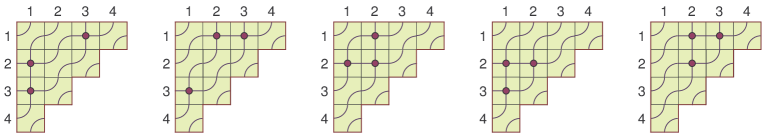
Figure 10.1. Graphs in  $\operatorname{{\text{RC}}}(1432)$  corresponding to the monomials $x_{1}x_{2}x_{3}$ ,  $x_{1}^{2}x_{3}$ ,  $x_{1}x_{2}^{2}$ ,  $x_{2}^{2}x_{3}$  and  $x_{1}^{2}x_{2}$ , in this order.

Polynomials  $\{\operatorname{\mathfrak{S}}_{w}\hskip 1.70709pt:\hskip 1.70709ptw\in S_{\infty}\}$  are known to form a basis in the ring  $\mathbb{Z}[x_{1},x_{2},\ldots]\hskip 0.85355pt.$ Schubert coefficients  are defined as structure constants:

$$\operatorname{\mathfrak{S}}_{u}\cdot\operatorname{\mathfrak{S}}_{v}\,=\,\sum_{w\in S_{\infty}}\hskip 1.70709ptc^{w}_{uv}\hskip 1.70709pt\operatorname{\mathfrak{S}}_{w}\hskip 0.85355pt.$$

It is known that  $c^{w}_{uv}\in\mathbb{N}$  for all  $u,v,w\in S_{\infty}$ .

Conjecture 10.1.

Schubert coefficients  $\{c^{w}_{uv}\hskip 1.70709pt:\hskip 1.70709ptu,v,w\in S_{\infty}\}$  are not in $\hskip 0.85355pt{{{\sf\#P}}}$.

For Grassmannian permutations (permutations with one descent), Schubert polynomial coincide with Schur polynomials, so Schubert coefficients generalize LR coefficients. This is a starting point of a number of further generalizations, see [Knu16, Kog01, MPP14].

10.2. Schubert–Kostka numbers

For a permutation  $w\in S_{n}$  and an integer vector  $a\in\mathbb{N}^{n}$, the Schubert–Kostka number  $K_{w\hskip 0.85355pta}:=[{\textbf{{x}}}^{a}]\operatorname{\mathfrak{S}}_{w}$  is the coefficient of a monomial in the Schubert polynomial. By definition,  $\{K_{w\hskip 0.85355pta}\}\in{\textsf{\#P}}$.

Proposition 10.2 (Morales).

Schubert coefficients $\big{\{}c^{w}_{uv}\hskip 1.70709pt:\hskip 1.70709ptu,v,w\in S_{\infty}\big{\}}$  are in  ${\sf{GapP}}$.

Proof.

Let  $\sigma\in S_{n}$  and let  $\rho_{n}:=(n-1,\ldots,1,0)\in\mathbb{N}^{n}$. Define

$$\Omega(\sigma)\hskip 1.70709pt:=\hskip 1.70709pt\big{\{}(a,b,c)\in(\mathbb{N}^{n})^{3}\hskip 1.70709pt:\hskip 1.70709pta+b+c=\sigma\rho_{n}\big{\}}.$$

It was shown by Postnikov and Stanley in [PS09, Cor. 17.13], that

$$c^{w}_{uv}\,=\,\sum_{\sigma\in S_{n}}\,\sum_{(a,b,c)\hskip 1.70709pt\in\hskip 1.70709pt\Omega(\sigma)}\,\text{\rm sign}(\sigma)\hskip 1.70709ptK_{u\hskip 0.85355pta}\hskip 1.70709ptK_{v\hskip 0.85355ptb}\hskip 1.70709ptK_{w\hskip 0.85355ptc}\hskip 1.70709pt.$$

Separating positive and negative signs shows that  $\{c^{w}_{uv}\}\in{\textsf{\#P}}-{\textsf{\#P}}$, as desired. ∎

Following [PS09, $\S$17], define the Schubert–Kostka matrix  $\widehat{\textbf{{K}}}=\bigl{(}K_{u\hskip 0.85355pta}\bigr{)}$, which naturally generalizes the Kostka matrix  $\textbf{{K}}=\bigl{(}K_{\lambda\mu}\bigr{)}$. Similarly, define the inverse  ${\widehat{\textbf{{K}}}}^{-1}=\bigl{(}K^{-1}_{a\hskip 0.85355ptu}\bigr{)}$  which generalizes the inverse Kostka matrix  $\textbf{{K}}^{-1}=\bigl{(}K^{-1}_{\lambda\mu}\bigr{)}$.

Proposition 10.3.

The inverse Schubert–Kostka numbers $\big{\{}K^{-1}_{a\hskip 0.85355ptu}\hskip 1.70709pt:\hskip 1.70709pta\in\mathbb{N}^{\infty},\hskip 1.70709ptu\in S_{\infty}\big{\}}$  are in  ${\sf{GapP}}$.

Similarly to the previous proposition, the result follows directly from the identity in [PS09, Prop. 17.3]. One can ask if the absolute values $\big{\{}\big{|}K^{-1}_{a\hskip 0.85355ptu}\big{|}\big{\}}$  are in #P. Conjecture 7.10 implies that the answer is negative, but perhaps this more general problem is an easier place to start.

10.3. Has the problem been resolved?

There are two issues around Conjecture 10.1 worth mentioning, as both, in different ways, suggest that the conjecture has already been resolved in the negative (i.e. a combinatorial interpretation has already been found).

First, Izzet Coskun in [Cos+] claimed to have completely resolved the problem of finding combinatorial interpretations for Schubert coefficients using the technology of Mondrian tableaux. Earlier, he used Mondrian tableaux to give a combinatorial interpretation for step-two Schubert coefficients (corresponding to permutations with at most two descents) in [Cos09] extending Vakil’s earlier work [Vak06], see a discussion in [CV09].

Unfortunately, paper [Cos+] has not been peer reviewed and has been largely ignored by the community (see [Bil21] for a notable exception). We should mention that the state of art recent work [KZ17] gives a tiling combinatorial interpretation for the step-three Schubert coefficients. It seems, we are nowhere close to resolving Conjecture 10.1 in full generality.

Second, Sara Billey suggested in [Bil21], that Schubert coefficients already have a “combinatorial interpretation”, since by definition they are equal to the number of irreducible components in certain intersections of three Schubert varieties, and thus “they already count something”. Can one create a #P function out of this definition?

While it is true that Schubert coefficients count the number of certain points in $\mathbb{C}^{n}$, these points are not necessarily rational. In fact, they are usually roots of a large system of rational polynomials. On the other hand, Billey and Vakil prove in [BV08, $\S$4], that there are some remarkable pathologies for these intersections related to realizability and stretchability of pseudoline arrangements. It follows from the Mnëv universality theorem [Mnëv88] (see also [Shor91]), that these problems are $\exists\mathbb{R}$-complete.

The  $\exists\mathbb{R}$  complexity class is in  PSPACE  and not expected to have polynomial size verifiers. This suggests that in the worst case, Billey’s approach needs a superexponential precision with which one would want to compute the intersection points (i.e. the floating point computation needs superpolynomially many digits), implying that it is unlikely that there exists a poly-time verifier in this case.

The issue is not too different from that of Kronecker coefficients, which can be written as  $g(\lambda,\mu,\nu)=\dim\big{(}\SS^{\lambda}\otimes\SS^{\mu}\otimes\SS^{\nu}\big{)}^{S_{n}}$. Thus, one can argue that they count basis vectors in this space of invariants. But since the Kronecker coefficients can be exponential in $n$, see e.g. [PPY19], how would one present such a basis so it can be verified (or at least read) in poly-time?

10.4. Elements of style

There are both cultural and mathematical reasons why the type of issues we discuss in $\S$9.4 do not apply to the study of Schubert coefficients, so let us quickly address the differences.

Schubert polynomials were originally introduced by Lascoux and Schützenberger in 1980s in the geometric context, see [Las95]. They remain deeply entrenched in the area which offers a melange of tools nonexistent on the combinatorial and representation theoretic side. Arguably, this resulted in a deeper study with a long series of achievements, too long to outline in this survey (see e.g. [Knu22]).

By now, the Schubert theory outgrew the “combinatorial interpretation issue” as its raison d’être. Arguably, the area was always about developing the theory to understand the geometry of flag varieties from a combinatorial point of view (cf. [LS85]).

This brings us to the curious case of puzzles, a type of tilings on a triangular lattice with labeled edges (see e.g. [Knu16]). Aesthetically pleasing for sure, is there some additional value such combinatorial interpretation bring to the study?

To us, the answer is a mixture. On the one hand, when the set of tiles is finite they clearly define a combinatorial interpretation. Having a nice or highly symmetric set of tiles can be convenient to prove structural results about vanishing and other properties of the numbers, cf. [KT99].

On the other hand, there is nothing surprising in the labeled tiles from the computational point of view. By adding new labels, one can always break them into single triangles, which can then be viewed as a variation on Wang tiles  [Wang61]. The latter can also be broken into triangles leading to the same model of computation. Wang’s celebrated insight is that such tilings are just as powerful as Turing machines. In fact, the example of Wang tilings with the boundary was one of Levin’s six original NP-complete problems [Lev73].

And yet, there is a clear computational difference between various types of increasing tableaux (such as set-valued tableaux) vs. puzzles. While the former need some memory to check which numbers appear, the latter can be verified by checking only local label conditions (think of finite state automata), making the puzzles (slightly) less powerful as a computational model. Part of the weakness here comes from the fixed triangular region space requirement, further constraining the puzzle tiling model.

11. The magic of the symmetric group

Before we can explain why, in our view, so many numbers in Algebraic Combinatorics are not in #P, we need to deconstruct the wonderful world of the symmetric group. Only after reducing all the great features to just one, we can fully appreciate its power as well as its limitation.

11.1. Pruning down the list

We start with representation theoretic point of view, demystifying some of the magic. All these results are routine and well known, so we restrict ourselves to quick pointers to the literature.

$(a)$   $f^{\lambda}\hskip 1.70709pt|\hskip 1.70709ptn!$  This is non-specific to $S_{n}$, since the dimension  $\chi(1)$  of an irreducible character of a finite group $G$ always divides the order $|G|$, see e.g. [Ser77, $\S$6.5].

$(b)$   $\{f^{\lambda}\}\in{{{\sf\#P}}}.$  This is a consequence of  $\chi^{\lambda}\downarrow^{S_{n}}_{S_{n-1}}$  having a simple spectrum, i.e. multiplicities at most one. Irreducibles in the restriction (given by the branching rule) correspond to removing a corner from Young diagram $\lambda$. Iterating the restrictions along the subgroup chain  $S_{n}\supset S_{n-1}\supset\ldots\supset S_{1}$  implies that  $f^{\lambda}=|\operatorname{{\rm SYT}}(\lambda)|$, cf. [OV96].

$(c)$   $\sum_{\lambda\vdash n}\hskip 1.70709pt(f^{\lambda})^{2}=n!$  This is non-specific to $S_{n}$. Burnside’s identity  $\sum\chi(1)^{2}=|G|$  holds for all finite groups, cf. Remark 8.2.

$(d)$   $\chi^{\lambda}(\mu)\in\mathbb{Z}$.  This is follows from a property of conjugacy classes of $S_{n}$, that  $\sigma^{k}\in[\mu]$  for every  $\sigma\in[\mu]$  and  $(k,\text{ord}(\sigma))=1$, see e.g. [Ser77, $\S$13.1]. See also $\S$8.2 for references to row and column sums of character tables of general finite groups.

$(e)$   $\{$Irreps of $S_{n}\}$  $\longleftrightarrow$  {Irreps of ${\text{\rm GL}}(N)$}.  This is a direct consequence of the Schur–Weyl duality:  $S_{n}\times{\text{\rm GL}}(N)$  act on  $(\mathbb{C}^{N})^{\otimes n}$  and the action has simple spectrum  $\SS^{\lambda}\otimes V_{\lambda}$  of tensor products of corresponding irreps, see e.g. [FH99, $\S$6.2].

$(f)$   $\{K_{\lambda\mu}\}\in{{{\sf\#P}}}$.  This is a direct consequence of the highest weight theory for  ${\text{\rm GL}}(N)$. Indeed, the induced product for $S_{n}$ reps corresponds to the tensor product of ${\text{\rm GL}}(N)$ reps, via $(e)$. Now use the definition  $K_{\lambda\mu}=\big{\langle}\chi^{\lambda},1\uparrow_{S_{\mu_{1}}\times S_{\mu_{2}}\times\cdots}^{S_{n}}\big{\rangle}$.

$(g)$   $\{f^{\lambda}\}\in{{\sf FP}}$.  This extension of $(b)$ is a consequence of  dimensions  $\dim(V_{\lambda})$  of ${\text{\rm GL}}(N)$  irreps given by a product. The latter is computed as a ratio of two Vandermonde determinants. The product formula for  $f^{\lambda}=\dim(\SS^{\lambda})$  follows by taking the limit, see e.g. [Sta99, $\S$7.21].

11.2. Hook-length formula

The results above are both fundamental in the area and have conceptual proofs explaining away some of the magic. The hook-length formula (HLF) (see $\S$7.1) may also seem fundamental at first, until one realizes that all proofs are a byproduct of calculations highly specific to symmetric groups. Here is a quick overview of the proofs:

$\circ$  Direct cancelation proof via the product formula in $\S$11.1 $(g)$, see the original proof

in [FRT54], see also [Sta99, $\S$7.21].

$\circ$  NPS bijection [NPS97], an intricate argument seemingly based on the jeu-de-taquin,

but neither using its properties nor originally motivated by it (see e.g. [Sag01, $\S$3.10]).

$\circ$  Hillman–Grassl bijection [HG76], see also [Kra99a] (plus a limit argument, see e.g. [Pak01]),

an elegant bijection that is equivalent to RSK, see [Gan81], [PV10, $\S$6.5] and [VW83, $\S$5].

$\circ$  Geometric bijection (plus a limit argument) in [Pak01], obtained as a deconstruction

of RSK via local transformations (cf. [Hop14]).

$\circ$  Lagrange interpolation inductive arguments, see [Ban08, GN04, Kir92, Ver92]. These

are elementary analytic proofs which require the most calculation.

$\circ$  GNW hook walk [GNW79], a ingenuous argument which embeds the Lagrange inter-

polation inductive argument in probabilistic disguise as shown by Kerov [Ker93].

$\circ$  Inductive proof via bijection of the branching rule in [CKP11], obtained as a

combinatorial deconstruction of the GNW hook walk argument, cf. [Zei84].

$\circ$  Naruse HLF  [MPP17, MPP18a], an advanced generalization of the HLF which easily

implies it (see also [Kon20]). All currently known proofs are technically involved.

Neither of these proofs explains the HLF on a deeper level, since each of them either has a substantive computational part, or outsources the computation to RSK and its relatives.

11.3. Robinson–Schensted–Knuth correspondence

We argue that the RSK  is the one true miracle in the area. Let us count some of the ways it emerges, in historical order:

$\circ$  The (original) Robinson–Schensted algorithm, later extended by Knuth [Knu70].

$\circ$  The Burge correspondence [Bur74] (see also [Ful97, $\S$A.4.1]).

$\circ$  The Hillman–Grassl correspondence [HG76] (see above).

$\circ$  Schützenberger’s jeu-de-taquin [Schü77] (see also [Sag01, $\S$3.7]).

$\circ$  Viennot’s geometric construction [Vie77] (see also [Sag01, $\S$3.6]).

$\circ$  Quantum version of Désarménien’s straightening algorithm [Dés80] given in [LT96].

$\circ$  Steinberg’s unipotent variety approach [Ste88] (see also [vL00]).

$\circ$  Fomin’s growth diagrams approach [Fom95] (see also [Sta99, $\S$7.13]).

$\circ$  Benkart–Sottile–Stroomer tableau switching [BSS96].

$\circ$  Our geometric bijection [Pak01] (see above).

$\circ$  Lascoux’s double crystal graphs version [Las03].

$\circ$  The octahedral map [KTW04, DK05b] (see also [DK08, HK06, PV10, Spe07]).

There are many more versions of RSK — these are just the ones we find most interesting. There are also numerous extensions, generalizations and applications both in and outside of the area. Let us now clarify some items on this list.

Some of the bijections above, such as the geometric construction by Viennot and the double crystal graphs by Lascoux, are restatements of RSK into a different language. Several others require a serious proof that they coincide with RSK, e.g. the Hillman–Grassl correspondence and the jeu-de-taquin. In a difficult case, Désarménien’s straightening algorithm is similar but not equal to RSK, but the quantum versions do coincide.

In [PV10], we set up a technology which allow one to prove that various maps in the area are in fact linear time reducible to and from the RSK. This allows us to put the Schützenberger involution, the tableau switching and the octahedral recurrence on the list.

Now is the time to ask a key question: Given so many different approaches to so many different problems, why do they result in the same bijection? There is a formal mathematical reason to explain coincidences between any two RSK appearances. The explanations could be algebraic or combinatorial, but neither would resolve a question given the multitude of instances.

The answer is simple and unambiguous. It does not really matter what is the deep reason behind the RSK, whether it is the highest weight theory, the straightening algorithm or something else. What matters is that each RSK appearance is a shadow of one fundamental result that is yet to be formalized. This suggests we treat RSK as the one true miracle  which causes much of what we consider magical about the symmetric group.

11.4. LR rule

Consider the Littlewood–Richardson coefficients and its many combinatorial interpretations (see e.g. [vL01] for an extensive albeit dated survey):

${\small{\hskip 0.85355pt\diamond\hskip 0.85355pt}}$  The original LR rule:  $c^{\lambda}_{\mu\nu}=|\operatorname{{\rm LR}}(\lambda/\mu,\nu)|$, see [LR34].

${\small{\hskip 0.85355pt\diamond\hskip 0.85355pt}}$  The LR variation:  $c^{\lambda}_{\mu\nu}=|\operatorname{{\rm LR}}(\mu\circ\nu,\lambda)|$, see e.g. [RW84].

${\small{\hskip 0.85355pt\diamond\hskip 0.85355pt}}$  James–Peel pictures [JP79], see also [CS84, Zel81].

${\small{\hskip 0.85355pt\diamond\hskip 0.85355pt}}$  Gelfand–Zelevinsky interpretation using Gelfand–Tsetlin patterns [GZ85].

${\small{\hskip 0.85355pt\diamond\hskip 0.85355pt}}$  Leaves of the Lascoux–Schützenberger tree [LS85].

${\small{\hskip 0.85355pt\diamond\hskip 0.85355pt}}$  Kirillov–Reshetikhin rigged configurations [KR88] (see also [KSS02]).

${\small{\hskip 0.85355pt\diamond\hskip 0.85355pt}}$  Berenstein–Zelevinsky triangles [BZ92].

${\small{\hskip 0.85355pt\diamond\hskip 0.85355pt}}$  Fomin–Greene good maps [FG93].

${\small{\hskip 0.85355pt\diamond\hskip 0.85355pt}}$  Nakashima’s interpretation using crystal graphs [Nak93] (see also [BS17, $\S$9]).

${\small{\hskip 0.85355pt\diamond\hskip 0.85355pt}}$  Littelmann’s paths [Lit94].

${\small{\hskip 0.85355pt\diamond\hskip 0.85355pt}}$  Knutson–Tao hives [KT99], see also [GP00].

${\small{\hskip 0.85355pt\diamond\hskip 0.85355pt}}$  Kogan’s interpretation using RC-graphs [Kog01].

${\small{\hskip 0.85355pt\diamond\hskip 0.85355pt}}$  Buch’s set-valued tableaux [Buch02].

${\small{\hskip 0.85355pt\diamond\hskip 0.85355pt}}$  Knutson–Tao–Woodward puzzles [KTW04].

${\small{\hskip 0.85355pt\diamond\hskip 0.85355pt}}$  Danilov–Koshevoy arrays [DK05a].

${\small{\hskip 0.85355pt\diamond\hskip 0.85355pt}}$  Vakil’s chessgames [Vak06].

${\small{\hskip 0.85355pt\diamond\hskip 0.85355pt}}$  Thomas–Yong $S_{3}$-symmetric LR rule [TY08].

${\small{\hskip 0.85355pt\diamond\hskip 0.85355pt}}$  Purbhoo’s mosaics [Pur08] (see also [Zin09]).

${\small{\hskip 0.85355pt\diamond\hskip 0.85355pt}}$  Coskun’s Mondrian tableaux [Cos09].

${\small{\hskip 0.85355pt\diamond\hskip 0.85355pt}}$  Nadeau’s fully packed loop configurations in a triangle [Nad13] (see also [FN15]).

The list above is so lengthy, it is worth examining carefully. Most of these LR rules are byproducts of (often but not always, successful) efforts to find a combinatorial interpretation of more general numbers. Some of these are closely related to each other, while others seem quite different, both visually and mathematically.

Now, on the surface the RSK is nowhere in the picture. We already mentioned [Ker84, Whi81, Zel81] which make the connection explicit, but here is a quick outline of how to get the original LR rule.

Start with a skew shape  $\lambda/\mu$, and run the jeu-de-taquin on  $\operatorname{{\rm SYT}}(\lambda/\mu)$. The number of times each  $A\in\operatorname{{\rm SYT}}(\nu)$  is the image  $\mathrm{jdt}\bigl{(}\operatorname{{\rm SYT}}(\lambda/\mu)\bigr{)}$  is exactly $c^{\lambda}_{\mu\nu}$, for all $A$ and $\nu$. Taking the lex-smallest such  $A$ (obtained by reading squares of $\nu$ left-to-right as commonly done), gives a combinatorial interpretation  $c^{\lambda}_{\mu\nu}=\big{|}\big{\{}B\in\operatorname{{\rm SYT}}(\lambda/\mu)\hskip 1.70709pt:\hskip 1.70709pt\mathrm{jdt}(B)=A\big{\}}\big{|}$.

While the above combinatorial interpretation suffices to show that $\{c^{\lambda}_{\mu\nu}\}\in{\textsf{\#P}}$, minor adjustments can be made to beautify the resulting rule. First, note that preimage of squares in every row of $A$ cannot be in the same column of  $B=\mathrm{jdt}^{-1}(A)$, so we can relabel $A$ by placing $i$ in the squares of $i$-th row. We get a unique  $A_{0}\in\operatorname{SSYT}(\nu,\nu)$. Now, the preimage in  $\operatorname{{\rm LR}}(\lambda/\mu,\nu):=\mathrm{jdt}^{-1}(A_{0})\subseteq\operatorname{SSYT}(\lambda/\mu,\nu)$  can be described using the ballot condition, giving the usual description of  $\operatorname{{\rm LR}}(\lambda/\mu,\nu)$.

We emphasize that RSK is omnipresent in the LR study [vL01]. It helps to approach this historically (we will try to be brief). The LR rule was introduced in [LR34]. Soon after, Robinson introduced the first version of RSK in his (incomplete) effort to prove the original LR rule [Rob38]. As James describes in [Jam87], the LR rule “is much harder to prove than was at first suspected.”

Macdonald [Mac95, $\S$I.9] credits Schützenberger [Schü77] and Thomas’s thesis [Tho74] with first complete proofs. Both were obtained in the context of RSK and its relatives. Since then, many proofs of the LR rule were discovered, too many to be cited here, all related to RSK relatives (ibid.) We single out the proof in [KTW04] based on the associativity property given by the octahedral map, and a geometry inspired proof in [BKT04] based on the jeu-de-taquin. Note that both use properties of RSK relatives.

Given that the role of RSK is often invisible without carefully examining the proofs of the LR interpretations above, this brings us to the following question: Are these “combinatorial interpretations” of LR coefficients equivalent in some formal sense?

11.5. Little boxes all the same

There are several ways to formalize the question above. First, note that all “combinatorial interpretations” above are naturally in #P, with the exception of crystal graphs which can have exponential size; the issue can be fixed if one follows the bijection in [NS11].

Second, all of these combinatorial interpretations are related to the original LR rule via a sequence of explicit poly-time bijections. For example, the LR tableaux are in bijection with: hives and BZ triangles [PV05], crystal graphs [NS11], Mondrian tableaux [Liu17], etc. This is unsurprising, perhaps, compared with parsimonious reductions between many #P-complete problems such as the number of $3$-colorings and the number of Hamiltonian cycles, see e.g. [Pap94b, $\S$18].

More surprising is that with few notable exceptions these bijections have linear time complexity. For example, when there is a natural presentation as integer points in polytopes, these polytopes are essentially the same and the bijection is given by a special linear map, see [PV05]. This holds for LR tableaux interpreted as GT patterns, as well as for hives, BZ triangles and DK arrays, where the natural presentation is binary, see [DP16, PV05].

It is thus most surprising, that RSK is behind so many other combinatorial interpretations, the bijection  $\operatorname{{\rm LR}}(\lambda/\mu,\nu)\to\operatorname{{\rm LR}}(\mu\circ\nu,\lambda)$  being the most natural such example. Recall the (algebraically obvious) fundamental symmetry  $c^{\lambda}_{\mu\nu}=c^{\lambda}_{\nu\mu}$, which is not transparent on the LR tableaux or the highly symmetric BZ triangles. Nor does it follow from integer points in polytopes of GT patterns since the GZ polytopes are asymmetric. In other words, proving  $|\operatorname{{\rm LR}}(\lambda/\mu,\nu)|=|\operatorname{{\rm LR}}(\lambda/\nu,\mu)|$  bijectively is rather nontrivial, and indeed is linear time equivalent to computing the RSK map as proved in [PV10].

Applying the fundamental symmetry can double the number of combinatorial interpretations, each time leading to a nontrivial bijections, see e.g. [ACM09] for puzzles and [TKA18] for hives. It follows from [PV10], that the RSK is behind them all. One can argue that the $S_{3}$-symmetric LR rule already has the fundamental symmetry “embedded” into the rule. But the way the rule is constructed, to verify that the combinatorial interpretation is valid one needs to perform the RSK.

Let us mention an experiment we made in [PV10, $\S$7], where we used ingredients from different bijections to cook up four$\hskip 1.70709pt(!)$ bijections proving the fundamental symmetry for LR tableaux. In the scientific method style, we conjectured all four to be identical without much of any checking [PV10, Conj. 1]. This conjecture is now completely proved by a combination of results in [DK05a] and [TKA18]. We followed the same approach to conjecture that two versions of the octahedral map coincide [PV10, Conj. 3]; this was later proved in [HK06].

Finally, we note a negative sort of evidence: as soon as one needs a different kind of combinatorial interpretation for the LR coefficients which does not involve the RSK, nothing emerges. This is why both Open Problems 7.8 and 7.9 are so challenging, cf. $\S$9.2$\hskip 0.85355pt{}({\ddagger})$.

11.6. What gives?

Combinatorics of the symmetric group is so vast, it is easy to get lost. There are thousands of papers, hundreds of bijections, and dozens of combinatorial interpretations which we cannot possibly mention here for the lack of space and limited lifespan. And yet, we claim that there is a unifying principle for a large part of the field.

Fundamentally, the Algebraic Combinatorics is the study of bases in symmetric spaces via combinatorics of transition matrices between them. The dimensions of these symmetric spaces tends to be exponential (think $S_{n}$ irreps, tensor powers, cohomology ring of Grassmannians, etc.) Thus, we need to be able to handle not only the exponential size bases, but also the exponential size of vectors in these bases.

In fact, most natural bases of these spaces do have vectors with exponential size support (think Young bases, Schur functions, Schubert polynomial, etc.) Fortunately, the components of the whole vector can often be computed from name of the vector (think of semistandard Young tableaux from Young diagrams for Schur functions, or RC-graphs from permutations). The coefficients are not necessarily positive (e.g. tabloids in the Young basis of $S_{n}$ irreps can have alternating signs), which is why given a choice it is best to use positive bases, e.g. work with Schur functions rather than Young bases.

Now, when applying operations to our symmetric spaces, one needs to be able to extract the standard symmetric bases out of these new large spaces. Since one cannot work with exponential size vectors, the symmetry must be traded for a concise presentation of the lex-smallest vector (in principle, any orbit representative of the underlying group of symmetries). For example, this easily leads to standard Young tableaux as lex-smallest vectors among tabloids of a given shape, see e.g. [Sag01, $\S$1.6]. We refer to [KR84] for more on this philosophy from the Invariant Theory point of view.

To see a more interesting example, consider the left-right action of  $G\times G$  on  $\mathbb{C}[G]$, which has a simple spectrum as the sum of  $\pi\otimes\pi$  over all irreducibles. For  $G=S_{n}$  one is then tempted to look for how lex-smallest components of vectors in the invariant subspaces of  $\mathbb{C}[S_{n}]$, leading to the straightening that Rota liked to much. The details behind the RSK correspondence and the LR rule are more technical, but the underlying story is similar and not much more complicated. And as we emphasize earlier, this all comes down to the miracle of RSK and its relatives.

What is amazing here is not that the resulting algorithm is nice and interrelated, but that it is correct. The former is a property of the underlying algebra, while the latter is a combinatorial miracle behind RSK. We don’t need to work hard to imagine a world where RSK does not exists – the (original) straightening is not in poly-time, or at least not obviously so (this is due to unexpected sign cancellations). If not for the Schur–Weyl duality we could be stuck there for a long time, at least until a quantum version was discovered.

For a more recent example, consider a interesting story of three papers by Thomas–Yong [TY18] and Pechenik–Yong [PY17a, PY17b], where the authors first introduce a generalization of jeu-de-taquin to obtain some combinatorial interpretation for the theory they wanted, and then developed another generalization of jeu-de-taquin to prove the desired combinatorial interpretation (conjectured earlier by Knutson and Vakil, see [CV09, $\S$5]).

We finish this section on a positive note. If one wants to find a combinatorial interpretation for Kronecker coefficients, in my opinion one would need to find an appropriate generalization of RSK. It is even clear how to start — the map should be from 3-dim contingency arrays into triples of semistandard Young tableaux, so that the number of elements in preimage is always  $g(\lambda,\mu,\nu)$, which would then have a combinatorial interpretation as the number of certain contingency arrays.

The idea would be to exploit the generalized Cauchy identity

$$\prod_{i,\hskip 0.85355ptj,\hskip 0.85355ptk}\hskip 1.70709pt\frac{1}{1\hskip 1.70709pt-\hskip 1.70709ptx_{i}\hskip 0.85355pty_{j}\hskip 0.85355ptz_{k}}\ =\ \sum_{\lambda,\hskip 0.85355pt\mu,\hskip 0.85355pt\nu}\hskip 1.70709ptg(\lambda,\mu,\nu)\hskip 1.70709pts_{\lambda}({\textbf{{x}}})\hskip 0.85355pts_{\mu}({\textbf{{y}}})\hskip 0.85355pts_{\nu}({\textbf{{z}}})$$

(see e.g. [Mac95, Exc. I.7.10] and [Sta99, Exc. 7.78]). Unfortunately, the structure of such arrays is more complicated than in the 2-dim case of contingency tables, so finding lex-smallest (under the action of the triple products of symmetric groups) does not appear to be feasible in full generality. Thus, unsurprisingly, until now this approach is worked out only in a few special cases where lex-smallest contingency arrays are easy to distinguish, see e.g. [Val00] and [IMW17, $\S$2].

12. How to prove a negative?

By the title of this section we mean: How to prove that a given function does not have a combinatorial interpretation? Unfortunately, we really can’t, at least not unconditionally. For all we know, it could be that  ${\textsf{P}}={\textsf{NP}}={\textsf{PSPACE}}$  and  ${\textsf{FP}}={\textsf{\#P}}$. In that case, poly-time verifiers can do magic, not just give combinatorial interpretations. Now that we accepted the need for some complexity assumptions, we can proceed to discussing special cases.

12.1. Nothing comes from nothing

Let  $f:\{0,1\}^{\ast}\to\mathbb{N}$  be a function. There is always a mathematical reason  why we have  $f(x)\in\mathbb{N}$  for all  $x\in\{0,1\}^{\ast}$. This reason could be an easy consequence from the definition, an observation, a routine calculation, a standard result in the area, or a technically difficult theorem. Whether this reason can be replaced by a counting argument  is exactly the same as asking if  $f\in{\textsf{\#P}}$.

Consider some examples. For  $f(x)=2^{|x|}$, the combinatorial interpretation is “all subsets of $[n]$,” where $n=|x|$ is the length of the word $x$. For  $f(x)=x(x-1)(x-2)/3$, the combinatorial interpretation is “all $3$-subsets of $[x]$ counted twice”. Here the (easy) number theoretic result  “$3\hskip 0.85355pt|\hskip 0.85355ptm(m-1)(m-2)$  for all $m\in\mathbb{N}$”  is proved by a counting argument.

In the other direction, for  $f(x)=2^{x}$, there is no combinatorial interpretation since the function is doubly exponential in the size of the input. There is still a (trivial) counting argument  here, placing this function in a counting class  #EXP, but that goes outside the scope of this survey.

Next, consider a polynomial  $\varphi(x)=(x-1)^{2}$  and let  $f\in{\textsf{\#P}}$. The function  $\varphi(f)$  is trivially nonnegative and in  ${\textsf{GapP}}={\textsf{\#P}}-{\textsf{\#P}}$. However, there is no natural combinatorial interpretation in this case, as we already discussed in $\S$3.2$\hskip 0.85355pt{}(4)$. There, we used a substitution  $x\leftarrow h(G):=\#$Hamiltonian cycles in graph $G$. Note that if we used a different substitution  $x\leftarrow e(P):=\#$linear extensions of a poset $P$,  then $(x-1)^{2}\in{\textsf{\#P}}$, see $\S$3.2$(1)$. This mean that the inequality  $(x-1)^{2}\geq 0$  may be trivial analytically, but cannot be proved by a counting argument in the worst case even if it can be proved in special cases, as this example shows.

Back to the LR and Kronecker coefficients, there is a very clear algebraic reason why we have  $c^{\lambda}_{\mu\nu}\geq 0$  and  $g(\lambda,\mu,\nu)\geq 0$. Fundamentally, it is reduced to the (easy) inequality  $\langle\zeta,\xi\rangle\geq 0$  for every two characters  $\zeta,\xi$  of a finite group $G$. It seems unlikely that this general inequality would have a proof based on a counting argument.

Now note that we have a really good understanding why LR coefficients are in #P, and a very poor understanding what why Kronecker coefficients are not (thus, Conjecture 9.1). As we mentioned above, it is neither unusual nor surprising that an inequality can be in #P is some special cases and not in others. Unfortunately, at the moment, the Kronecker coefficients are much too unapproachable to admit a resolution of the problem.

In summary, we are concerned not so much with whether any particular function is in #P, although we do care about that. Instead, we examine what proof ingredients (of general results) can be shown to be in #P, and refute those which are not. This is the subject of our long and technical paper [IP22]. In this section we present a brief and non-technical introduction.

12.2. Polynomials

A rational polynomial  $\varphi\in\mathbb{Q}[x]$  is called integer-valued  if  $\varphi(x)\in\mathbb{Z}$  for all  $t\in\mathbb{Z}$. It is well known and easy to see that  $\varphi$  is integer-valued if and only if  $\varphi$  is an integer linear combination of binomials:  $\varphi\in\mathbb{Z}\big{\langle}1,x,\tbinom{x}{2},\tbinom{x}{3},\ldots\big{\rangle}$. See e.g. [CC16] for the background and many related results.

Polynomials  $\varphi$  in the semigroup  $\mathbb{N}\big{\langle}1,x,\tbinom{x}{2},\tbinom{x}{3},\ldots\big{\rangle}$  are called binomial-good (binomial-bad, otherwise). Binomial-good polynomials have a combinatorial interpretation for $\varphi(x)$. Formally, for every function  $f\in{\textsf{\#P}}$, the function  $\varphi(f)$  is also in #P. For example, let  $f\leftarrow h(G)$  be the number of Hamiltonian cycles in $G$, and let  $\varphi(x)=\frac{1}{3}\hskip 0.85355ptx(x-1)(x-2)$. Then we have  $\varphi(f)=2\binom{f}{3}\in{\textsf{\#P}}$  as discussed above, since  $\varphi(f)$  counts twice the number of triples of distinct Hamiltonian cycles in $G$.

Let us emphasize that the combinatorial interpretation of $\varphi(f)$ is oblivious, i.e. it works with the verifier for the function $f$ as a black box without ever looking at the graph $G$ or the notion of Hamiltonicity. Note that the black box is not allowed to compute $f$, and all it can do is give a combinatorial interpretation for $f$. In other words, the black box verifier for $f$ looks at  $x\in\{0,1\}^{\ast}$  and says Yes/No in poly-time, and the verifier for $\varphi(f)$ works the same way by calling on the verifier for $f$.

Denote by  ${\mathcal{B}}$  the set of binomially-good polynomials, and by  ${\mathcal{O}}$  the set of polynomials which have an oblivious combinatorial interpretation. From above, ${\mathcal{B}}\subseteq{\mathcal{O}}$. It was proved in [HVW95, Thm 3.13] (see also [IP22, $\S$4.3]), that  ${\mathcal{B}}={\mathcal{O}}$, i.e. we show that binomial-bad polynomials $\varphi$ cannot have oblivious combinatorial interpretation. For example,  $\varphi=(x-1)^{2}=2\binom{x}{2}-x+1$  is binomial-bad, and for  $f\leftarrow h(G)$  we do not expect a combinatorial interpretation.

We also generalize this result to multivariate polynomials, where  $\varphi\in\mathbb{Q}[x_{1},\ldots,x_{k}]$  is integer-valued if  $\varphi\in\mathbb{Z}\big{\langle}\tbinom{x_{1}}{d_{1}}\cdots\tbinom{x_{k}}{d_{k}}\big{\rangle}$, see [Nag19]. By analogy with the univariate case, we say that $\varphi$ is binomial-good if  $\varphi\in\mathbb{N}\big{\langle}\tbinom{x_{1}}{d_{1}}\cdots\tbinom{x_{k}}{d_{k}}\big{\rangle}$, and prove   ${\mathcal{B}}={\mathcal{O}}$  for this generalization [IP22, $\S$4.3].

Denote by  ${\mathcal{C}}$  the set of polynomials  $\varphi\in\mathbb{Q}[x_{1},\ldots,x_{k}]$  such that  $\varphi(f_{1},\ldots,f_{k})\in{\textsf{\#P}}$  for all  $f_{1},\ldots,f_{k}\in{\textsf{\#P}}$. Clearly, ${\mathcal{O}}\subseteq{\mathcal{C}}$. Our Binomial Basis Conjecture (BBC) states that  ${\mathcal{O}}={\mathcal{C}}$, see [IP22, $\S$4.4]. Since this conjecture implies  ${\textsf{P}}\neq{\textsf{NP}}$ (ibid.), there is little hope to resolve it even in the univariate case. Thus, from the computational complexity point of view, the “combinatorial interpretation problem” for polynomials is completely resolved.

Example 12.1.

Let $\varphi:=(x-y)^{2}$. Clearly,  $\varphi(x,y)=2\binom{x}{2}+2\binom{y}{2}-2xy+x+y\notin{\mathcal{B}}$, which implies that  $\varphi\notin{\mathcal{C}}$. Consider the classical geometric proof of  $a^{2}+b^{2}\geq 2ab$  obtained by reflection of triangles as in Figure 12.1. Since reflected triangles cover both $a\times b$ rectangles, the inequality follows. The reader might want to ponder (before reading the footnote), why does this construction not give an oblivious combinatorial interpretation?

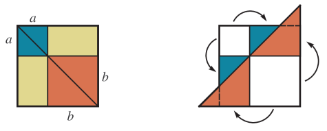
Figure 12.1. Geometric proof of the inequality  $a^{2}+b^{2}\geq 2ab$. Here the blue and red triangles are reflected to completely cover yellow rectangles.

12.3. Making weaker assumptions

For some polynomials and some #P functions, the BBC can be replaced by a weaker complexity theoretic assumption. To explain what is going on, we need a few definitions.

Let $f,g:\{0,1\}^{\ast}\to\mathbb{Z}$  be two #P functions. We say that  $f$  has a parsimonious reduction to $\hskip 0.85355ptg$, if there is a polynomial reduction  $\{0,1\}^{\ast}\to\{0,1\}^{\ast}$  which maps $f$ into $g$. Typically, if $f$ and $g$ count the number of solutions to problem $A$ and $B$, the parsimonious reduction preserves the number of solutions.

It is known, for example, that  #SAT  has a parsimonious reduction to  #HamiltonianCycles (and vise versa). This means that for every SAT formula $\Phi$, there is a polynomially constructed graph $G$, such that the number of satisfying assignments of $\Phi$ is equal to $h(G)$, see e.g. [Pap94b, $\S$18]. The same holds for  # 3Colorings,  #WangTilings, and many other #P-complete functions. For the lack of a better name, we call such #P functions counting-complete, and use  CCF  to denote the set of such functions.

On the other hand, unless ${\textsf{P}}={\textsf{NP}}$, the function #PerfectMatchings is not in CCF, since the corresponding vanishing problem  $\text{{\rm PM}}(G)=^{?}0$  is in P. The same holds for #LinearExtensions. So while these two functions are #P-complete, they are not counting-complete.

A map  $\varphi:\mathbb{N}^{k}\to\mathbb{Q}$  is called monotone if  $\varphi(a_{1},\ldots,a_{k})\leq\varphi(a_{1}^{\prime},\ldots,a_{k}^{\prime})$  for all integer  $a_{1}\leq a_{1}^{\prime}$, …, $a_{k}\leq a_{k}^{\prime}$. For example, polynomials  $x/2$,  $x-1$  and  $x+y$  are monotone, but  $x^{2}-2x$  and  $(x-y)^{2}$  are not. Denote by  ${\mathcal{M}}$  the set of monotone polynomials, and note that  ${\mathcal{B}}\subset{\mathcal{M}}$.

We can now state two results which allow weakening of the “oblivious” assumption:

(1)  Let $\varphi(x,y)=(x-y)^{2}\notin{\mathcal{O}}$. We prove a stronger claim in this case, that  $\varphi\notin{\mathcal{C}}$  unless a standard complexity assumption fails. Formally, we prove in [IP22, $\S$2.3], that for every two (independent) functions  $f,g\in{\textsf{CCF}}$, we have  $\varphi(f,g)\notin{\textsf{\#P}}$  unless  $\Sigma_{2}^{\textsc{p}}={\textsf{PH}}$.

This is the strategy used in [IPP22] to prove Theorem 8.1. Recall that by MN rule, the character  $\chi^{\lambda}(\mu)\in{\textsf{GapP}}$, so it can be written as  $(f-g)$  for some (usually, not independent) functions  $f,g\in{\textsf{\#P}}$. We found some instances of  $(\lambda,\mu)$, for which the corresponding $(f,g)$ are both independent and counting-complete. This implied the result. We believe the same approach could potentially work for Conjecture 7.10.

(2)  Let  $\varphi\in\mathbb{Q}[x_{1},\ldots,x_{k}]$  be a non-monotone polynomial, so  $\varphi\notin{\mathcal{B}}$. We prove a stronger claim in this case, that  $\varphi\notin{\mathcal{C}}$  unless a standard complexity assumption fails. Formally, let  $f_{1},\ldots,f_{k}\in{\textsf{CCF}}$  be independent counting-complete  #P  functions. We prove in [IP22, $\S$2.3], that  $\varphi(f_{1},\ldots,f_{k})\notin{\textsf{\#P}}$  unless  ${\textsf{UP}}={\textsf{coUP}}$, see [IP22, $\S$2.4]. In particular,  $(f-1)^{2}\notin{\textsf{\#P}}$  unless  ${\textsf{UP}}={\textsf{coUP}}$, cf. $\S$3.2$\hskip 0.85355pt{}(4)$.

For another example, recall the Motzkin polynomial  $M(x,y):=x^{2}y^{4}+x^{4}y^{2}-3x^{2}y^{2}+1$. It follows from the AM-GM inequality applied to positive terms, that  $M(x,y)\geq 0$  for all $x,y\in\mathbb{R}$. On the other hand, this polynomial is famously not a sum of squares, and is a fundamental example in Semidefinite Optimization, see e.g. [Ble13, Mar08]. Now, observe that  $M(x,y)$  is not monotone:  $M(0,1)=1$  and  $M(1,1)=0$. This gives  $M\notin{\mathcal{C}}$  unless  ${\textsf{UP}}={\textsf{coUP}}$.

Note that non-monotone polynomial  $(x-y)^{2}$  has a stronger property:  $(x-y)^{2}\psi\notin{\mathcal{M}}$, for all  $\psi\in\mathbb{Z}[x,y]$. By contrast, the multiple  $(x-1)^{2}\cdot x=6\tbinom{x}{3}+2\tbinom{x}{2}\in{\mathcal{B}}$  is binomial-good, and thus monotone.

12.4. Algebraic inequalities

Let  $\varphi,\hskip 0.85355pt\psi\in\mathbb{Q}[t_{1},\ldots,t_{k}]$, so that  $\varphi\leq\psi$  for all $(t_{1},\ldots,t_{k})\in\mathbb{N}^{k}$. Suppose that polynomial  $(\psi-\varphi)\in{\textsf{\#P}}$  and has an oblivious combinatorial interpretation. From above, we have  $(\psi-\varphi)$  is binomial-good. Since inequalities are routine building blocks across mathematics, it is worth examining which of them are binomial good.

First, note that the inequality  $a^{2}+b^{2}\geq 2ab$  is equivalent to the complete square case $(1)$ above. In [IP22, $\S$7.1], we show that a number of standard inequalities are also not in #P (in a sense of substitutions), including the Cauchy inequality, the Minkowski inequality, and the Alexandrov–Fenchel inequality. All these proofs are routine and similar to our proof of Proposition 5.4.

Let us single out the Hadamard inequality for real $d\times d$ matrices:

$$\det\begin{pmatrix}a_{11}&\cdots&a_{1d}\\ \vdots&\ddots&\vdots\\ a_{d1}&\cdots&a_{dd}\end{pmatrix}^{2}\ \leq\ \prod_{i=1}^{d}\hskip 1.70709pt\bigl{(}a_{i1}^{2}\hskip 0.85355pt+\hskip 0.85355pt\ldots\hskip 0.85355pt+\hskip 0.85355pta_{id}^{2}\bigr{)}\hskip 0.85355pt.$$

Geometrically, it says that the volume of a parallelepiped in $\mathbb{R}^{d}$ is at most the product of its basis edge lengths, with equality when these edges are orthogonal. Note that the standard proof use eigenvalues, see e.g. [HLP52, $\S$2.13] and [BB61, $\S$2.11], suggesting that translation into combinatorial language would be difficult.

Denote by  $H_{d}\big{(}a_{11},\ldots,a_{dd}\big{)}$  the polynomial defined by the Hadamard inequality. Note that $H_{2}(a,b,c,d)\in{\mathcal{C}}$, since

$$H_{2}(a,b,c,d)\,=\,(a^{2}\hskip 0.85355pt+\hskip 0.85355ptb^{2})(c^{2}\hskip 0.85355pt+\hskip 0.85355ptd^{2})\hskip 1.70709pt-\hskip 1.70709pt\det\begin{pmatrix}a&b\\ c&d\end{pmatrix}^{2}\,=\,(ac\hskip 0.85355pt+\hskip 0.85355ptbd)^{2}.$$

On the other hand,  $H_{2}(a,b,c,-d)\geq 0$  has different properties from our point of view. Indeed, we have  $H_{2}(a,b,c,-d)=(ac-bd)^{2}\notin{\mathcal{C}}$  unless  $\Sigma_{2}^{\textsc{p}}={\textsf{PH}}$. Finally, observe that

$$H_{3}{\begin{pmatrix}x&\binom{x}{3}&0\\ 0&1&1\\ 1&0&1\end{pmatrix}}\ =\ 3\hskip 0.85355pt\tbinom{x}{1}\hskip 1.70709pt+\hskip 1.70709pt6\hskip 0.85355pt\tbinom{x}{2}\hskip 1.70709pt-\hskip 1.70709pt3\hskip 0.85355pt\tbinom{x}{3}\hskip 1.70709pt+\hskip 1.70709pt28\hskip 0.85355pt\tbinom{x}{4}\hskip 1.70709pt+\hskip 1.70709pt90\hskip 0.85355pt\tbinom{x}{5}\hskip 1.70709pt+\hskip 1.70709pt60\hskip 0.85355pt\tbinom{x}{6}\,\notin{\mathcal{B}}\hskip 0.85355pt.$$

By the BBC, we have  $H_{3}\notin{\mathcal{C}}$. Since  $H_{3}\in{\mathcal{M}}$, this is the best we can prove with our tools.

12.5. Algebraic inequalities restricted to semialgebraic sets

In many cases, one is interested in polynomial inequalities where the variables are themselves constrained by a system of polynomial inequalities and equations. Our Diagonalization Theorem [IP22, Thm 6.2.1] gives a complete algebraic characterization of such systems with an oblivious combinatorial interpretation.

The results in [IP22] are both technical to state, difficult to prove and hard to apply. Instead of presenting or even outlining them here, we discuss two examples (one easy and one difficult) which give a glimpse at our arguments.

(1)  The Ahlswede–Daykin (AD) inequality, see e.g. [AS16, $\S$6.1], for  $n=1$  states:

$$\left\{\hskip 0.85355pt\begin{aligned} &x_{0}\hskip 0.85355pty_{0}\hskip 1.70709pt\leq\hskip 1.70709ptu_{0}\hskip 0.85355ptv_{0}\ ,\ x_{0}\hskip 0.85355pty_{1}\hskip 1.70709pt\leq\hskip 1.70709ptu_{0}\hskip 0.85355ptv_{1}\\ &x_{1}\hskip 0.85355pty_{0}\hskip 1.70709pt\leq\hskip 1.70709ptu_{0}\hskip 0.85355ptv_{1}\ ,\ x_{1}\hskip 0.85355pty_{1}\hskip 1.70709pt\leq\hskip 1.70709ptu_{1}\hskip 0.85355ptv_{1}\end{aligned}\right.\quad\Longrightarrow\quad(x_{0}+x_{1})(y_{0}+y_{1})\hskip 1.70709pt\leq\hskip 1.70709pt(u_{0}+u_{1})(v_{0}+v_{1})\hskip 0.85355pt,$$

for all  $x_{i},y_{i},u_{i},v_{i}\geq 0$, where  $i\in\{0,1\}$. We prove in [IP22, Prop. 2.5.1], that the AD inequality does not have an oblivious combinatorial interpretation. In other words, we prove that  $\varphi\notin{\mathcal{O}}$, where  $\varphi\hskip 0.85355pt:=\hskip 0.85355pt(u_{0}+u_{1})(v_{0}+v_{1})\hskip 0.85355pt-\hskip 0.85355pt(x_{0}+x_{1})(y_{0}+y_{1})$  restricted to the above system of four inequalities. Below is the outline of the proof.

Following [IP22, $\S$7.4], we rewrite the inequality in terms of #P functions as follows:

$$\left\{\hskip 0.85355pt\begin{aligned} &\alpha_{0}\beta_{0}+\xi_{1}=\gamma_{0}\delta_{0}\,,\ \alpha_{0}\beta_{1}+\xi_{2}=\gamma_{0}\delta_{1}\\ &\alpha_{1}\beta_{0}+\xi_{3}=\gamma_{0}\delta_{1}\,,\ \alpha_{1}\beta_{1}+\xi_{4}=\gamma_{1}\delta_{1}\end{aligned}\right.\ \ \Longrightarrow\ \ (\gamma_{0}+\gamma_{1})(\delta_{0}+\delta_{1})\hskip 0.85355pt-\hskip 0.85355pt(\alpha_{0}+\alpha_{1})(\beta_{0}+\beta_{1})\in{\textsf{\#P}}\hskip 0.85355pt,$$

for all  $(\alpha_{0},\alpha_{1},\beta_{0},\beta_{1},\gamma_{0},\gamma_{1},\delta_{0},\delta_{1},\xi_{1},\xi_{2},\xi_{3},\xi_{4})\in({\textsf{\#P}})^{12}$.  Second, make the following substitution into these 12 functions:  $\bigl{(}1,1,x,x,x,1,1,x,0,2\binom{x}{2},2\binom{x}{2},0\bigr{)}$  and check that the above system of inequalities is satisfied. Now let  $x\leftarrow f$, where  $f\in{\textsf{\#P}}$. This substitution gives  $\varphi(f)=(f-1)^{2}\notin{\mathcal{B}}$, and thus  $\varphi\notin{\mathcal{O}}$.

(2)  Let  $\textbf{{a}},\textbf{{b}}\in\mathbb{R}^{n}$ be weakly decreasing, such that  $\textbf{{a}}\trianglerighteq\textbf{{b}}$, see $\S$7.2. The Karamata inequality says for every convex function  $F:\mathbb{R}^{n}\to\mathbb{R}$, we have  $F(\textbf{{a}})\geq F(\textbf{{b}})$, see e.g. [HLP52, $\S$3.17] and [BB61, $\S$28, $\S$30]. We refer to [BP21, PPS20] for some recent applications to linear extensions and Young tableaux, and to [MOA11] for numerous generalizations and further references.

Following [IP22, $\S$7.5], we rewrite the inequality in the language of #P functions. Suppose

$$f_{1}\hskip 1.70709pt+\hskip 1.70709pt\ldots\hskip 1.70709pt+\hskip 1.70709ptf_{i}\,=\,g_{1}\hskip 1.70709pt+\hskip 1.70709pt\ldots\hskip 1.70709pt+\hskip 1.70709ptg_{i}\hskip 1.70709pt+\hskip 1.70709pth_{i}\quad\text{for all \ \ $1\leq i\leq n$,}$$

where  $f_{i},g_{i},h_{i}\in{\textsf{\#P}}$, and  $h_{n}=0$. Suppose also that

$$f_{i}\,=\,f_{i+1}\hskip 1.70709pt+\hskip 1.70709ptd_{i}\hskip 1.70709pt,\quad g_{i}\,=\,g_{i+1}\hskip 1.70709pt+\hskip 1.70709pte_{i}\hskip 1.70709pt,\quad\text{for all \ \ $1\leq i<n$,}$$

where  $d_{i},e_{i}\in{\textsf{\#P}}$. Finally, let  $\gamma:\mathbb{Z}\to\mathbb{N}$  be a nonnegative convex function. The Karamata function  $K^{n}_{\gamma}$  is defined as

$${\text{\text{K}}}^{\langle n\rangle}_{\gamma}(f_{1},\dots,f_{n},g_{1},\ldots,g_{n})\,:=\,\sum_{i=1}^{n}\hskip 1.70709pt\gamma(f_{i})\,-\,\sum_{i=1}^{n}\hskip 1.70709pt\gamma(g_{i})\hskip 1.70709pt.$$

Clearly,  ${\text{\text{K}}}^{\langle n\rangle}_{\gamma}\in{\textsf{GapP}}$  and nonnegative by the Karamata theorem. It is thus an interesting question if  ${\text{\text{K}}}^{\langle n\rangle}_{\gamma}\in{\mathcal{O}}$, i.e. if  ${\text{\text{K}}}^{\langle n\rangle}_{\gamma}(f_{1},\ldots,g_{n})\in{\mathcal{O}}$, i.e. in #P  for all  $f_{i},g_{i},h_{i},d_{i},e_{i}\in{\textsf{\#P}}$.

For example, for  $\gamma(t)=\alpha t+\beta$, we have  ${\text{\text{K}}}^{\langle n\rangle}_{\gamma}=0$. Similarly,

$${\text{\text{K}}}^{\langle 2\rangle}_{\gamma}(f_{1},f_{2},g_{1},g_{2}) =\,(e_{1}+h_{1})\hskip 0.85355pth_{1}\hskip 1.70709pt\in\hskip 1.70709pt{\textsf{\#P}}\quad\text{for}\ \ \gamma(t)=\tbinom{t}{2},\quad\text{and}$$

$${\text{\text{K}}}^{\langle 3\rangle}_{\gamma}(f_{1},f_{2},f_{3},g_{1},g_{2},g_{3}) =\,(d_{1}+e_{1})\hskip 0.85355pth_{1}\hskip 1.70709pt+\hskip 1.70709pt(d_{2}+e_{2})\hskip 0.85355pth_{2}\hskip 1.70709pt\in\hskip 1.70709pt{\textsf{\#P}}\quad\text{for}\ \ \gamma(t)=t^{2}.$$

It follows from here that  $2\hskip 0.85355pt{\text{\text{K}}}^{\langle 3\rangle}_{\gamma}\in{\mathcal{O}}$  where  $\gamma(t)=\tbinom{t}{2}$, since linear terms cancel out. We prove in [IP22, Prop. 7.5.5], that  ${\text{\text{K}}}^{\langle 3\rangle}_{\gamma}\notin{\mathcal{O}}$  for  $\gamma(t)=\binom{t}{2}$. The proof requires a computation of lattice points in a $12$-dimensional polytope defined by linear equations and inequalities corresponding to constraints on  $f_{i},g_{i},h_{i},d_{i},e_{i}$.

12.6. What’s next?

By now the (exhausted) reader knows what kind of results we want to prove — the many  “not in #P”  conjectures throughout the paper. And they know how we imagine the plan of attack — by simulating the proofs of positivity and integrality of these combinatorial functions with polynomial equations.

There are two main obstacles on the way. First, the proof of positivity and integrality can be rather involved, so distilling a single reason and expressing it as a polynomial inequality can be difficult. Naturally, one would want to start with counting graphs and linear extensions rather than Kronecker and Schubert coefficients, as the former seem much more generic and less involved. It may take a long time before this project can reach the latter.

Second, the family of polynomials for which we know that they don’t have an oblivious combinatorial interpretations is rather large and seems satisfactory for applications. But to make the final results more accessible and convincing to the general audience, it is important to weaken the assumptions (see $\S$12.3). This direction is certainly worth exploring in the context of Computational Complexity.

13. Counting complexity addendum

13.1. We need a list

Throughout the whole survey we tried to mention  ${{{\sf\#P}}}$-completeness  and  ${{{\sf\#P}}}$-hardness  as little as possible. There are two reasons for that: we wanted not to distract the reader from the main problem (membership in #P), and we wanted to minimize the confusion that invariably arises.

There is, however, a direct connection to these complexity classes. As we mention in $\S$2.6, we have  ${\textsf{FP}}\subseteq{\textsf{\#P}}$, which makes combinatorial interpretation of problems in  FP  trivial. Naturally, we are thus interested in problems that are not in FP. The best evidence that a function is not in  FP  yet potentially in  #P, is if a function is #P-hard. This is why it is worth checking #P-hardness of functions in every conjecture and open problem that we pose (cf. $\S$15.2).

If this was about NP-completeness, we would stop here and refer to [GJ79] along with some recent comprehensive list of NP-complete problems (such as this one on Wikipedia). Unfortunately, there does not seem to be such comprehensive sources about #P-completeness. Thus we present an annotated short list of such results, restricted only to functions which we consider relevant to the survey.

13.2. Graph theory problems

We proceed roughly according to the sections in this survey.

1. #Monotone 2SAT is #P-complete but $\notin{\textsf{CCF}}$. This implies that #VertexCover is #P-complete [Val79a].

2. #HamiltonianCycles is #P-complete [Val79a]. Moreover #HC is in CCF, since the proof is based on a parsimonious bijection. In the context of Smiths’s theorem (see $\S$3.2), this remains true for #HC in cubic planar graphs [LOT03].

3. #3Colorings is #P-complete [Val79a]. Moreover #3C is in CCF, since the proof is based on a parsimonious bijection.

4. #PerfectMatchings is #P-complete via reduction to Permanent [Val79c]. This implies that #$k$-Matchings  $\{p(G,k)\}$ is #P-complete (see $\S$5.1). Thus,  $\{f(G,k)\}$ is #P-hard by telescoping. The problem remains #P-complete for subgraphs in $\mathbb{Z}^{3}$ [Val79b], and even for the number of 3-dim domino tilings [PY13]. For planar graphs #PerfectMathings is in FP by the Kasteleyn formula, see e.g. [LP86, $\S$8.3].
   The vanishing problem  $\{\text{{\rm PM}}(G)=^{?}0\}$  is in P, see e.g. [LP86, $\S$9.1].

5. #SpanningForests  $\{F(G,k)\}$ is #P-complete (see $\S$5.3). This holds because the total number of spanning forests  $1+F(G,1)+\ldots+F(G,n-1)=T(G;2,1)$  is an evaluation of the Tutte polynomial  known to be #P-complete, see e.g. [Wel93, Thm 6.2.9]. This implies that $\{f(G,k)\}$ is #P-hard. For a fixed $k\geq 1$, both  $\{F(G,k)\}$  and  $\{F(G,n-k)\}$  are in FP [Myr92].

6. #SpanningSubgraphs  is  #P-complete [PB83]. This is an evaluation of the Tutte polynomial (see e.g. [Bol98, Ch. X]). We conjecture that the function in Conjecture 5.6 is  #P-hard.

7. IsingModelStatisticalSum  is  #P-complete [JS93, Thm 15]. In notation of $\S$5.7, this and Proposition 5.9 implies that  $\{\mathrm{Cor}(v,w)\}$  is #P-complete. For planar graphs, the problem is in FP  by the Kasteleyn–Fisher determinant formula  [Kas63, Fis66].

8. For general rational hyperplane arrangements, the problem of counting the number of regions in the complement is #P-complete. For membership in #P, see $\S$4.1. The hardness follows from graphical arrangements where the number of regions equal to the evaluation  $|\chi_{G}(-1)|$  of the chromatic polynomial (see e.g. [Sta99, $\S$3.11, Exc. 94-95]). This evaluation is equal to the number of acyclic orientations of $G$, known to be #P-complete, see e.g. [Wel93, Thm 6.2.9].

9. #LinearExtensions  $\{e(P)\}$  are #P-complete [BW91]. Thus, the function defined by the Björner–Wachs inequality is #P-complete (see $\S$6.1). By telescoping, the function defined by the Stanley inequality is #P-hard (see $\S$6.3). Computing  $e(P)$  remains #P-complete for $P$ of height two, and of width two [DP18]. The function defined by the Sidorenko inequality (see $\S$6.2) is conjectured to be #P-complete in [CPP22b, $\S$9.6].

10. #WangTilings  of a square is #P-complete; this follows e.g. from the proof of Thm 3 in [DD07] that the decision problem in NP-complete.

11. Volume is #P-hard via reduction to #LinearExtensions of order polytope [BW91],
    remains #P-hard for zonotopes [DGH98].
    MixedVolume is #P-hard for boxes via reduction to Permanent (ibid.)

13.3. Algebraic combinatorics problems with binary input

The type of input makes so much difference for problems in Algebraic Combinatorics, we decided to separate them altogether and make a clear indication in the name, so they would be impossible to confuse.

Note that if the problem is in FP in the binary input, then this is also true in the unary input. Vice versa, if the problem is #P-complete or #P-hard in the unary input, then this is also true in the binary input. Similar claims hold for the decision problems as well.

1. ContingencyTablesBinaryInput  $\{{\text{\rm T}}(\lambda,\mu)\}$  is  #P-complete even for  $\ell(\lambda)=2$  [DKM97].
   The vanishing problem  $\{{\text{\rm T}}(\lambda,\mu)>^{?}0\}\in{\textsf{P}}$, since it is equivalent to  $\{|\lambda|=^{?}|\mu|\}$.
   When  $\ell(\lambda)$  is fixed, the problem has FPTAS [G+11].
   When  $\ell(\lambda),\ell(\mu)$  are fixed, the problem is in FP by [Bar93].

2. KostkaBinaryInput  $\{K_{\lambda\mu}\}$  is  #P-complete [Nar06].
   The vanishing problem  $\{K_{\lambda\mu}>^{?}0\}\in{\textsf{P}}$, since it is equivalent to  $\{\lambda\trianglerighteq^{?}\mu\}$, see $\S$7.2.
   The uniqueness problem  $\{K_{\lambda\mu}=^{?}1\}\in{\textsf{P}}$, see a complete characterization in [BZ90].

3. LittlewoodRichardsonBinaryInput  $\{c^{\lambda}_{\mu\nu}\}$  is  #P-complete [Nar06].
   The vanishing problem  $\{c^{\lambda}_{\mu\nu}>^{?}0\}\in{\textsf{P}}$, see [DM06, MNS12].
   The uniqueness problem  $\{c^{\lambda}_{\mu\nu}=^{?}1\}\in{\textsf{P}}$. More generally, $\{c^{\lambda}_{\mu\nu}=^{?}t\}\in{\textsf{P}}$  
   for every fixed $t\geq 0$, see [Ike12, Thm 11.3.2] and [Ike16].

4. KroneckerBinaryInput  $g(\lambda,\mu,\nu)$  is  #P-hard. This follows easily from the result that  Littlewood-RichardsonBinaryInput is  #P-complete, and trivially from the unary case.
   The vanishing problem  $\{g(\lambda,\mu,\nu)>^{?}0\}$  is NP-hard; this follows trivially from the unary case.

5. ReducedKroneckerBinaryInput  $\{\overline{g}(\alpha,\beta,\gamma)\}$  is  #P-hard, same reason as above.
   We conjecture that the vanishing problem  $\{\overline{g}(\alpha,\beta,\gamma)>^{?}0\}$  is in NP-hard.

6. ExcitedDiagrams  $\{|{\mathcal{E}}(\lambda/\mu)|\}\in{\textsf{FP}}$  via reduction to flagged tableaux  [MPP18a, Cor. 3.7].
   This is the number of terms of the summation in the NHLF. The vanishing problem is trivial.

7. CharacterSquaredBinaryInput  $\big{\{}(\chi^{\lambda}(\mu))^{2}\big{\}}$  is doubly exponential and thus
   not in PSPACE. For example, $\chi^{\lambda}(1)={\text{\rm Cat}}(m)=e^{\Omega(n)}$, where  $\lambda=(m,m)$  and  $n=2m$.
   The vanishing problem  $\{\chi^{\lambda}(\mu)\neq^{?}0\}$  is  NP-hard [PP17, $\S 7$]; a stronger result follows
   from the unary case.

8. HurwitzBinaryInput  $\{h_{g\mu}\}$  is doubly exponential and thus not in PSPACE.
   For example, $h_{0\hskip 0.85355pt(n)}=n^{n-2}$.

13.4. Algebraic combinatorics problems with unary input

This is the most interesting case, and the one we discuss throughout the paper. To minimize the overlap, we don’t include here some of the poly-time result which hold already for the binary case.

1. ContingencyTablesUnaryInput  $\{{\text{\rm T}}(\lambda,\mu)\}$  is not known to be  #P-complete,
   see [DO04, $\S$1.1] and [PP17, $\S$8.1]. We conjecture this to be true.
   When  $\ell(\lambda)$  is fixed the problem is not  #P-complete unless  ${\textsf{P}}={\textsf{NP}}$.

2. KostkaUnaryInput  $\{K_{\lambda\mu}\}$  is not known to be  #P-complete [PP17, $\S$8.1].
   We conjecture this to be true. This would follow from the conjecture that
   #ContingencyTablesUnaryInput is #P-complete, via the reduction in [Nar06].
   Moreover, we conjecture that  $\big{\{}K_{\lambda\hskip 0.85355pt(2^{a}1^{b})}\big{\}}$  is #P-complete.

3. LittlewoodRichardsonUnaryInput  $\{c^{\lambda}_{\mu\nu}\}$  is conjectured to be  #P-complete [PP17, $\S$8.1]. This would follow from the conjecture that  KostkaUnaryInput is  #P-complete, via the reduction in [Nar06]. The vanishing problem  has a recursive description, see [Zel99, Prop. 9].
   The vanishing  of generalized LR coefficients (tileability using Knutson–Tao puzzles
   regions in the triangular lattice with given boundary), is NP-complete [PY14].

4. KroneckerUnaryInput  $g(\lambda,\mu,\nu)$  is  #P-hard. This follows from [IMW17].
   The vanishing problem  $\{g(\lambda,\mu,\nu)>^{?}0\}$  is NP-hard, ibid.
   We conjecture that  $\{g(\lambda,\lambda,\lambda)\hskip 1.70709pt:\hskip 1.70709pt\lambda=\lambda^{\prime}\}$  is #P-hard, cf. Conjecture 9.2 and [PP22],
   and that  $\{g(\lambda,\lambda,\mu)\hskip 1.70709pt:\hskip 1.70709pt\mu=(n-k,k)\}$  is also #P-hard, cf. Remark 9.3 and [PP14].

5. ReducedKroneckerUnaryInput  $\overline{g}(\alpha,\beta,\gamma)$  is  #P-hard [PP20b].
   The vanishing problem  $\{\overline{g}(\alpha,\beta,\gamma)>^{?}0\}$  is conjectured to be  NP-hard in [PP20b, $\S$4.4].

6. CharacterSquaredUnaryInput  $\big{\{}(\chi^{\lambda}(\mu))^{2}\big{\}}$  is #P-hard [Hep94],
   and  $(\chi^{\lambda}(\mu))^{2}\notin{\textsf{\#P}}$  unless  $\Sigma_{2}^{\textsc{p}}={\textsf{PH}}$, see Theorem 8.1.
   The vanishing problem  $\{\chi^{\lambda}(\mu)=^{?}0\}$  is  ${{\sf C_{=}P}}$-complete, and thus NP-hard [IPP22].
   The positivity problem  $\{\chi^{\lambda}(\mu)\geq^{?}0\}$  is  $\operatorname{PP}$-complete, and thus PH-hard, ibid.

7. InverseKostkaUnaryInput  $\big{\{}K^{-1}_{\lambda\mu}\big{\}}$  has not been studied. We conjecture it is #P-hard.
   For the vanishing problem  $\{K^{-1}_{\lambda\mu}=^{?}0\}$, we conjecture it is  ${{\sf C_{=}P}}$-complete (cf. Conjecture 7.10).

8. BruhatOrderIdeal  $\{B(\sigma)\}$, where  $B(\sigma):=|\{\omega\in S_{n}\hskip 1.70709pt:\hskip 1.70709pt\omega\preccurlyeq\sigma\}|$, is  #P-complete [DP18].
   This problem is equivalent to  #LinearExtensions  for permutation posets:  $B(\sigma)=e(P_{\sigma})$.

9. ReducedFactorizations  $\{r(w)\hskip 1.70709pt:\hskip 1.70709ptw\in S_{n}\}$ [Sta84], are defined as

   $$\qquad r(w)\hskip 1.70709pt:=\hskip 1.70709pt\#\big{\{}\hskip 0.85355pt(i_{1},\ldots,i_{\ell})\,:\,(i_{1},i_{1}+1)\cdots(i_{\ell},i_{\ell}+1)=w,\hskip 1.70709pt1\leq i_{j}<n,\hskip 1.70709pt\ell=\operatorname{{\rm inv}}(\omega)\hskip 0.85355pt\big{\}}.$$

   The problem is conjectured to be  #P-complete [DP18, $\S$8.5], cf. [MPY22, $\S$6]. When  $w\in S_{n}$
   is vexillary ($2143$-avoiding), we have  $\{r(w)\}\in{\textsf{FP}}$  from [Man01, Cor. 2.8.2] and the HLF.

10. SchubertCoefficient  $c^{w}_{uv}$  is not known to be #P-hard. We conjecture this to be true.
    The vanishing problem  $\{c^{w}_{uv}>^{?}0\}$  is not knows to be  NP-hard [ARY13, $\S$4].

11. SchubertKostka  $\{K_{ua}\}$  and  #RC-graphs  $\{\operatorname{\mathfrak{S}}_{u}(1)=\sum_{a}K_{ua}\}$  have not been studied.
    We conjecture that both are  #P-complete.

12. IncreasingTableaux  $\big{\{}g^{\lambda}:=|\operatorname{{\rm IT}}(\lambda)|\big{\}}$, where an increasing tableau  $A\in\operatorname{{\rm IT}}(\lambda)$  is a plane partition strictly increasing in rows and columns, and no gaps between $1$ and maximal entry of $A$, see [TY09]. Note that  $g^{\lambda}\geq f^{\lambda}$. This problem  $\{g^{\lambda}\}$  was proposed in [TY11, $\S$1.3], and conjectured to be #P-complete in [MPP22, $\S$7.10].

13. SetValuedTableaux  $\big{\{}s(\lambda,k):=|\operatorname{{\rm SVT}}(\lambda,k)|\big{\}}$, where a set-valued tableau  $A\in\operatorname{{\rm SVT}}(\lambda,k)$  is a surjection from  $[k]$  to squares of Young diagram $\lambda$, s.t. the numbers increase in rows and columns of the image, see [Buch02]. Complexity of  $\{s(\lambda,k)\}$  was asked in [MPY22, $\S$5.2] and [H+22, $\S$5.7]. We conjecture that  $\{s(\lambda,k)\}$  is #P-complete.

14. HurwitzNumberUnaryInput  $\{h_{g\mu}\}$  is #P-complete [PP22+].

13.5. Related problems

Here are a few additional problems we think are worth solving (all in unary).

1. Let  $\Lambda\subset\mathbb{N}^{3}$  be a 3-dim Young diagram. Denote by  $P_{\Lambda}$  the corresponding poset. We conjecture that  $\{e(P_{\Lambda})\}$  is  #P-complete. In fact, we conjecture this holds for  $\Lambda$  of height two.

2. Let  $\Lambda\subset\mathbb{N}^{3}$  be a 3-dim Young diagram. We conjecture that the number of domino tilings of $\Lambda$ is  #P-complete. Again, we conjecture this holds for  $\Lambda$  of height two.

3. Let  $\mathcal{A}=(A_{1},\ldots,A_{n})$  and  $\mathcal{B}=(B_{1},\ldots,B_{n})$  be two collections of points in $\mathbb{N}^{3}$. Denote by  $f(\mathcal{A},\mathcal{B})$  the number of collections  $(\gamma_{1},\ldots,\gamma_{n})$  of nonintersecting shortest paths  $\gamma_{i}:A_{i}\to B_{i}$,  $1\leq i\leq n$. We conjecture that  $\big{\{}f(\mathcal{A},\mathcal{B})\big{\}}$  is #P-complete.

4. Let  ${\text{\rm F}}(d_{1},\ldots,d_{n})$  be the number of simple graphs with given degree sequence. We conjecture that  $\{{\text{\rm F}}(d_{1},\ldots,d_{n})\}$  is #P-complete. For many related results and further references, see e.g. [Wor18]. The vanishing problem  $\{{\text{\rm F}}(d_{1},\ldots,d_{n})>^{?}0\}$  is in P even in binary, by the Erdős–Gallai theorem (see e.g. [AL05]).

5. Let  $G\subset S_{n}$  be a permutation group given by its generators. Recall that the size  $|G|$, the size of the commutator  $|[G,G]|$  and many other functions are in FP, see e.g. [Ser03]. What about the number  $c(G)$  of conjugacy classes?

6. We conjecture that tileability of simply-connected regions in $\mathbb{R}^{2}$ with the unit square and the unit edge equilateral triangle is NP-complete (rotations are allowed, see [Zin09, App. 1]), and that the number of such tilings is #P-complete.

7. Let  $Q\subset\mathbb{R}^{2}$  be a centrally-symmetric polygon with integer side lengths, and let $T$ is a fixed set of rhombi tiles with unit sides. We conjecture that the number of tilings of $Q$ with $T$ is #P-complete. Note that the existence of such tilings is in P, see e.g. [KS92]. We refer to [Ken93, $\S$5] and [Pak03, $\S$5.3, $\S$7] for some background.

8. We conjecture that for binary matroids  represented by vectors in $\mathbb{F}_{2}^{n}$, the number of bases is #P-complete. Note that for paving matroids  represented by cycles, and for bicircular matroids, the number of bases is #P-complete, see [Jer06, $\S$3] and [GN06, $\S$3].

14. Proofs

14.1. Proof of Proposition 4.2

Let $\mathcal{T}_{n}$ be the set of rooted plane triangulations on $n$ vertices, and let $b_{n}:=|\mathcal{T}_{n}|$. Here the root in a triangulation $G=(V,E)$ is a flag $(v,e,F)$, where $v\in V$, $e=(v,w)\in E$ and $F$ is a face in $G$ containing $e$. Tutte’s product formula  shows that $\{b_{n}\}$ can be computed in poly$(n)$ time, see e.g. [Scha15]. Moreover, Poulalhon and Schaeffer [PS06] gave a bijective proof of Tutte’s formula, by constructing a bijection $\Phi:\mathcal{T}_{n}\to\mathcal{B}_{n}$ between rooted plane triangulations on $n$ vertices and certain balanced plane trees with two additional markings. It follows from the construction that both $\Phi$ and $\Phi^{-1}$ can be computed in $O(n)$ time.

Let $\Gamma={\text{\rm Aut}}(G)$ be the group of automorphisms of graph $G$. It is easy to see that the stabilizer subgroup ${\text{\rm Stab}}_{G}(v,e,F)=1$, because rooted triangulations have a unique topological embedding into a sphere. In particular, this implies that  $|\Gamma|\leq 4|E|=O(n)$. Recall that for all planar graphs, the effective graph isomorphism can be done in linear time [HW74]. In summary, for each $e^{\prime}=(v^{\prime},w^{\prime})\in E$, it can be decided in poly$(n)$ time whether there is an automorphism $g\in\Gamma$ s.t. $g\cdot v=v^{\prime}$ and $g\cdot w=w^{\prime}$. Moreover, when it exists such $g$ can be computed explicitly.

Now, a combinatorial interpretation for $\{a_{n}\}$ can be constructed as follows. Let $t\in\mathcal{B}_{n}$. Use the Depth First Search (DFS) around $t$ to obtain a unique labeling of vertices of $t$. Use $\Phi^{-1}$ to transferred this labeling onto $\tau:=\Phi^{-1}(t)\in\mathcal{T}_{n}$. Use the argument above to compute all $O(n)$ relabelings $\tau^{\prime}$ of $\tau$. For all such $\tau^{\prime}$, check if they are isomorphic to $\tau$, and if not discard such $\tau^{\prime}$. Compute $\Phi(\tau^{\prime})$ for all such rooted triangulations. We obtain exactly $|\Gamma\cdot\tau|=O(n^{2})$ balanced plane trees. Accept $t$ if it is lex-smallest, and reject otherwise. The details are straightforward. ∎

14.2. Proof of Proposition 8.6

Recall that  $\rho^{(n)}=1\uparrow_{C_{n}}^{S_{n}}\hskip 0.85355pt$, where $C_{n}\simeq\mathbb{Z}_{n}$ is the usual cyclic subgroup of $S_{n}$. Let  $\mu=(\mu_{1},\ldots,\mu_{\ell})\vdash n$  be a partition into distinct parts:  $\mu_{1}>\hskip 0.85355pt\ldots\hskip 0.85355pt>\mu_{\ell}>0$. We have:

$$\rho^{\mu} =\ 1\uparrow_{C_{\mu_{1}}\times\hskip 1.70709pt\cdots\hskip 1.70709pt\times C_{\mu_{\ell}}}^{S_{n}}\ =\ \rho^{(\mu_{1})}\otimes\hskip 1.70709pt\cdots\hskip 1.70709pt\otimes\rho^{(\mu_{\ell})}\uparrow_{S_{\mu_{1}}\times\hskip 1.70709pt\cdots\hskip 1.70709pt\times S_{\mu_{\ell}}}^{S_{n}}$$

$$=\ \sum_{\lambda\vdash n}\hskip 1.70709pt\Bigg{[}\sum_{\nu^{(1)}\vdash\mu_{1}}\hskip 1.70709pt\hskip 1.70709pt\ldots\hskip 1.70709pt\sum_{\nu^{(\ell)}\vdash\mu_{\ell}}\,c^{\lambda}_{\nu^{(1)},\hskip 1.70709pt\ldots\hskip 1.70709pt,\hskip 1.70709pt\nu^{(\ell)}}\,a_{\nu^{(1)}\hskip 0.85355pt(\mu_{1})}\hskip 1.70709pt\cdots\hskip 1.70709pta_{\nu^{(\ell)}\hskip 0.85355pt(\mu_{\ell})}\Bigg{]}\,\chi^{\lambda}\,,$$

where the generalized LR coefficient

$$c^{\lambda}_{\nu^{(1)},\hskip 1.70709pt\ldots\hskip 1.70709pt,\hskip 1.70709pt\nu^{(\ell)}}\ :=\ \sum_{\tau^{(1)},\ldots,\tau^{(\ell-2)}}\hskip 1.70709ptc^{\lambda}_{\nu^{(1)}\tau^{(1)}}c^{\tau^{(1)}}_{\nu^{(2)}\tau^{(2)}}\hskip 1.70709pt\cdots\hskip 1.70709ptc^{\tau^{(\ell-2)}}_{\nu^{(\ell-1)}\nu^{(\ell)}}$$

are written as sums of products of LR coefficients. Combining (KW) and the LR rule, this gives a (rather cumbersome) combinatorial interpretation of the multiplicity  $a_{\lambda\mu}$  of $\chi^{\lambda}$ . This is clearly in #P, which proves the first part. The second part follows from the same argument, with rows $(\mu_{i})$ replaced by rectangles with distinct lengths.∎

15. Final remarks

15.1.

The term combinatorial interpretation  seems to be relatively recent and was first used by Hardy [Har40, $\S$6.9], in connection with the Rogers–Ramanujan identities. There, the meaning was literal, to say that RR identities can be restated in a combinatorial language. The first modern usage was by Kaplansky and Riordan [KR46, p. 262], to say that Stirling numbers of second kind  have a “combinatorial interpretation” as the number of rook placements on the staircase shape.

Part of the reason is linguistic. For example, MacMahon used plenty of “interpretations” in his celebrated Combinatory Analysis [Mac15], so the term “combinatory interpretation” can be found in several papers, e.g. in [Ing26].

15.2.

There is a reason we are so cavalier with many #P-hardness conjectures in Section 13. Roughly speaking, this is because the universe of interesting combinatorial FP functions is quite small, and is reduced to:

• dynamic programming (see e.g. [CLRS09, $\S$15]),

• determinant formulas, e.g. (AFDF), the matrix-tree theorem (MTT), the Lindström–Gessel–Viennot theorem (LGV, see e.g. [GJ83, $\S$5.4.2]), and the Kasteleyn formula (cf. $\S$13.2),

• explicit formulas, e.g. (HLF) and MacMahon’s box formula (see e.g. Eq. (7.109) in [Sta99]).

If your function clearly does not belong to either of these (not well-defined) classes, there is a good chance it is not in FP. Although in principle there are are intermediate counting classes between FP and #P (unless ${\textsf{FP}}={\textsf{\#P}}$), in practice no one has seen them. Various dichotomy NP-completeness results only reinforce this belief, see e.g. classic paper [HL90] and the most recent breakthrough [Zhuk20]. In summary: If you don’t see how to compute a function using standard approaches, then most likely it is provably hard to do.

15.3.

We have used a lot of space presenting our arguments in support of our conjectures that many combinatorial functions in Algebraic Combinatorics are (probably) not in #P. Here is a quick summary of our arguments, TLDR style:

• Are you smarter than everyone?  So many people worked on these problems, if there was a combinatorial interpretation it would have been discovered by now.

• You can’t get there if you are going in the wrong direction.  If everyone in a community thinks a problem has a positive solution and they can’t even agree what would it mean to have a negative solution, there is a chance the problem never gets solved. At the very least the community should hedge and pursue both directions.

• There is already one miracle. Why are you expecting another one?  The LR rule and all its variations are magical. But they are caused by one true miracle: the RSK. All the variations on the theme (jeu-de-taquin, octahedral map, etc.), are equivalent in a formal sense, and thus simply the RSK in disguise. Given the scarcity of miracles, it seems unreasonable to hope for a positive solution without using the RSK or its relative in an essential way.

• Nothing comes from nothing.  The proof that a function is positive or integral is based on a sequence of arguments. For certain type of arguments that are given by algebraic inequalities, we can show they do not have oblivious combinatorial interpretations. So either your favorite function is very special and its proof avoids all such arguments, or you need another proof.

15.4.

While writing this survey, we had an unmistakable feeling of mapping the terra incognita. This reminded us of Nicolas Sanson’s 1650 map of North America, where the author made a logical leap and extend shore lines to create the Island of California, see below. You can imagine why he did it, but it’s still an important error which took about fifty years to correct. We can’t wait to find out if it’s us who are making unjustified logical leaps, or it’s others who have been using a wrong map. We just hope it will take less than fifty years.

Acknowledgements

We dedicate this survey to the memory of Gian-Carlo Rota whose teaching and philosophy influenced both our approach to the subject and our view of the world. We are embarrassed that it took so long for us to recognize his influence.

This paper would not exist without our recent work with Christian Ikenmeyer and our extensive collaboration with Greta Panova. We have also benefitted from closed collaboration with Swee Hong Chan, Sam Dittmer, Scott Garrabrant, Alejandro Morales, Danny Nguyen, Ernesto Vallejo, Jed Yang and Damir Yeliussizov. We are deeply grateful for the opportunity to work with them all.

We are also thankful for helpful discussions on the subject with Scott Aaronson, Olga Azenhas, Cyril Banderier, Sasha Barvinok, Sara Billey, Artëm Chernikov, Jesús De Loera, Michael Drmota, Éric Fusy, Pavel Galashin, Nikita Gladkov, Darij Grinberg, Josh Grochow, Leonid Gurvits, Zach Hamaker, Sam Hopkins, Mark Jerrum, Allen Knutson, Christian Krattenthaler, Greg Kuperberg, Svante Linusson, Tyrrell McAllister, Fëdor Petrov, Vic Reiner, Yair Shenfeld, Richard Stanley, Josh Swanson, Ramon van Handel, Dennis White, Nathan Williams, Alex Yong and Paul Zinn-Justin. We thank Vince Vatter for graciously sharing with us [Vat18].

Some of this material was accumulated over the years based on numerous conversations. We sincerely apologize to anyone we forgot to mention. The author was partially supported by the NSF.

References

- [Aar16] Scott Aaronson, , in Open problems in mathematics, Springer, Cham, 2016, 1–122; available at scottaaronson.com/papers/pnp.pdf
- [AHK18] Karim Adiprasito, June Huh and Eric Katz, Hodge theory for combinatorial geometries, Annals of Math. 188 (2018), 381–452.
- [AS18] Connor Ahlbach and Joshua P. Swanson, Cyclic sieving, necklaces, and branching rules related to Thrall’s problem, Electron. J. Combin. 25 (2018), Paper 4.42, 38 pp.
- [AS16] Noga Alon and Joel H. Spencer, The probabilistic method (Fourth ed.), John Wiley, Hoboken, NJ, 2016, 375 pp.
- [ALOV18] Nima Anari, Kuikui Liu, Shayan Oveis Gharan and Cynthia Vinzant, Log-concave polynomials III: Mason’s Ultra-log-concavity conjecture for independent sets of matroids, preprint (2018), 11 pp.; arXiv:1811.01600.
- [ARY13] David Anderson, Edward Richmond and Alexander Yong, Eigenvalues of Hermitian matrices and equivariant cohomology of Grassmannians, Compos. Math. 149 (2013), 1569–1582.
- [AB89] George E. Andrews and Rodney J. Baxter, A motivated proof of the Rogers–Ramanujan identities, Amer. Math. Monthly 96 (1989), 401–409.
- [AG88] George E. Andrews and Frank G. Garvan, Dyson’s crank of a partition, Bull. AMS 18 (1988), no. 2, 167–171.
- [AB09] Sanjeev Arora and Boaz Barak, Computational complexity. A modern approach, Cambridge Univ. Press, Cambridge, 2009, 579 pp.
- [A+98] Sanjeev Arora, Carsten Lund, Rajeev Motwani, Madhu Sudan and Mario Szegedy, Proof verification and the hardness of approximation problems, J. ACM 45 (1998), 501–555.
- [AL05] Richard Arratia and Thomas M. Liggett, How likely is an i.i.d. degree sequence to be graphical?, Ann. Appl. Probab. 15 (2005), 652–670.
- [AS54] Arthur O. L. Atkin and Peter Swinnerton-Dyer, Some properties of partitions, Proc. LMS 4 (1954), 84–106.
- [ACM09] Olga Azenhas, Alessandro Conflitti and Ricardo Mamede, On an index two subgroup of puzzle and Littlewood–Richardson tableau -symmetries, preprint DMUC. 09-51 (2009), 21 pp.; available at hdl.handle.net/10316/13627
- [Bab18] László Babai, Group, graphs, algorithms: the graph isomorphism problem, in Proc. ICM Rio de Janeiro, Vol. IV, World Sci., Hackensack, NJ, 2018, 3319–3336; see also arXiv:1512.03547.
- [Bab19] László Babai, Canonical form for graphs in quasipolynomial time, in Proc. 51st STOC (2019), 1237–1246
- [BL83] László Babai and Eugene M. Luks, Canonical labeling of graphs, in Proc. 15th STOC (1983), 171–183.
- [BE16] Kirby Baker and Edward Early, Character polynomials and row sums of the symmetric group, preprint (2016), 9 pp.; available at tinyurl.com/yxj5l7fd.
- [BO05] Cristina M. Ballantine and Rosa C. Orellana, A combinatorial interpretation for the coefficients in the Kronecker product , Sém. Lothar. Combin. 54A (2005), Art. B54Af, 29 pp.
- [Ban08] Jason Bandlow, An elementary proof of the hook formula, Electron. J. Combin. 15 (2008), no. 1, RP 45, 14 pp.
- [Bar93] Alexander Barvinok, A polynomial time algorithm for counting integral points in polyhedra when the dimension is fixed, Math. Oper. Res. 19 (1994), 769–779.
- [Bar07] Alexander Barvinok, Brunn–Minkowski inequalities for contingency tables and integer flows, Adv. Math. 211 (2007), 105–122.
- [Bax82] Rodney J. Baxter, Exactly solved models in statistical mechanics, Academic Press, London, 1982, 486 pp.
- [BB61] Edwin F. Beckenbach and Richard Bellman, Inequalities, Springer, Berlin, 1961, 198 pp.
- [BSS96] Georgia Benkart, Frank Sottile and Jeffrey Stroomer, Tableau switching: algorithms and applications, J. Combin. Theory, Ser. A 76 (1996), 11–43.
- [BBR06] François Bergeron, Riccardo Biagioli and Mercedes H. Rosas, Inequalities between Littlewood–Richardson coefficients, J. Combin. Theory, Ser. A 113 (2006), 567–590.
- [BB93] Nantel Bergeron and Sara Billey, RC-graphs and Schubert polynomials, Experiment. Math. 2 (1993), 257–269.
- [BZ88] Arkady D. Berenstein and Andrey V. Zelevinsky, Involutions on Gelfand–Tsetlin schemes and multiplicities in skew -modules, Soviet Math. Dokl. 37 (1988), 799–802.
- [BZ90] Arkady D. Berenstein and Andrey V. Zelevinsky, When is the multiplicity of a weight equal to ?, Funct. Anal. Appl. 24 (1990), no. 4, 259–269.
- [BZ92] Arkady D. Berenstein and Andrey V. Zelevinsky, Triple multiplicities for and the spectrum of the exterior algebra of the adjoint representation, J. Algebraic Combin. 1 (1992), 7–22.
- [BB04] Christine Bessenrodt and Christiane Behns, On the Durfee size of Kronecker products of characters of the symmetric group and its double covers, J. Algebra 280 (2004), 132–144.
- [BBS21] Christine Bessenrodt, Christopher Bowman and Louise Sutton, Kronecker positivity and 2-modular representation theory, Trans. AMS, Ser. B 8 (2021), 1024–1055.
- [BO04] Christine Bessenrodt and Jørn B. Olsson, On the sequence A085642, OEIS article (2004), 6 pp.; available at tinyurl.com/2mzt7m4x
- [Bil21] Sara Billey, Basic Schubert Calculus, Part 2, lecture at Combinatorial Algebraic Geometry Workshop, ICERM, Brown University, RI (February 1, 2021); full video and transcript are available at tinyurl.com/yn22dnue , slides are available at tinyurl.com/3vec4hrd
- [BJS93] Sara Billey, William Jockusch and Richard P. Stanley, Some combinatorial properties of Schubert polynomials, J. Algebraic Combin. 2 (1993), 345–374.
- [BV08] Sara Billey and Ravi Vakil, Intersections of Schubert varieties and other permutation array schemes, in Algorithms in algebraic geometry, Springer, New York, 2008, 21–54.
- [Bjö11] Anders Björner, A -analogue of the FKG inequality and some applications, Combinatorica 31 (2011), 151–164.
- [BW89] Anders Björner and Michelle L. Wachs, -hook length formulas for forests, J. Combin. Theory, Ser. A 52 (1989), 165–187.
- [Bla17] Jonah Blasiak, Kronecker coefficients for one hook shape, Sém. Lothar. Combin 77 (2017), Art. B77c, 40 pp.
- [Ble13] Grigoriy Blekherman, Nonnegative polynomials and sums of squares, in Semidefinite optimization and convex algebraic geometry, SIAM, Philadelphia, PA, 2013, 159–202.
- [BP21] Ivan A. Bochkov and Fedor V. Petrov, The bounds for the number of linear extensions via chain and antichain coverings, Order 38 (2021), no. 2, 323–328.
- [Bol98] Béla Bollobás, Modern graph theory, Springer, New York, 1998, 394 pp.
- [BBS99] Béla Bollobás, Graham Brightwell and Alexander Sidorenko, Geometrical techniques for estimating numbers of linear extensions, European J. Combin. 20 (1999), 329–335.
- [BS00] Mireille Bousquet-Mélou and Gilles Schaeffer, Enumeration of planar constellations, Adv. Appl. Math. 24 (2000), 337–368.
- [BDO15] Christopher Bowman, Maud De Visscher and Rosa Orellana, The partition algebra and the Kronecker coefficients, Trans. AMS 367 (2015), 3647–3667.
- [Brä15] Petter Brändén, Unimodality, log-concavity, real-rootedness and beyond, in Handbook of enumerative combinatorics, CRC Press, Boca Raton, FL, 2015, 437–483.
- [BH20] Petter Brändén and June Huh, Lorentzian polynomials, Annals of Math. 192 (2020), 821–891.
- [Bre73] Lev M. Bregman, Certain properties of nonnegative matrices and their permanents, Dokl. Akad. Nauk SSSR 211 (1973), 27–30.
- [Bre89] Francesco Brenti, Unimodal, log-concave and Pólya frequency sequences in combinatorics, Mem. AMS 81 (1989), no. 413, 106 pp.
- [Bre94] Francesco Brenti, Log-concave and unimodal sequences in algebra, combinatorics, and geometry: an update, in Jerusalem combinatorics, AMS, Providence, RI, 1994, 71–89.
- [BOR09] Emmanuel Briand, Rosa Orellana and Mercedes Rosas, Reduced Kronecker coefficients and counter-examples to Mulmuley’s strong saturation conjecture SH, Comput. Complexity 18 (2009), 577–600.
- [BOR11] Emmanuel Briand, Rosa Orellana and Mercedes Rosas, The stability of the Kronecker product of Schur functions, J. Algebra 331 (2011), 11–27.
- [BT02] Graham Brightwell and William T. Trotter, A combinatorial approach to correlation inequalities, Discrete Math. 257 (2002), 311–327.
- [BW00] Graham Brightwell and Douglas B. West, Partially ordered sets, Ch. 11 in Handbook of discrete and combinatorial mathematics, CRC Press, Boca Raton, FL, 2000, 717–752.
- [BW91] Graham Brightwell and Peter Winkler, Counting linear extensions, Order 8 (1991), 225–247.
- [Buch02] Anders S. Buch, A Littlewood–Richardson rule for the -theory of Grassmannians, Acta Math. 189 (2002), 37–78.
- [BKT04] Anders S. Buch, Andrew Kresch and Harry Tamvakis, Littlewood–Richardson rules for Grassmannians, Adv. Math. 185 (2004), 80–90.
- [BT00] David A. Buchsbaum and Brian D. Taylor, The straightening formula and the first and second fundamental theorems, in Gian-Carlo Rota (1932–1999), Notices AMS 47 (2000), 210–212.
- [BS17] Daniel Bump and Anne Schilling, Crystal bases, World Sci., Hackensack, NJ, 2017, 279 pp.
- [Bur74] William H. Burge, Four correspondences between graphs and generalized Young tableaux, J. Combin. Theory, Ser. A 17 (1974), 12–30.
- [BI08] Peter Bürgisser and Christian Ikenmeyer, The complexity of computing Kronecker coefficients, in Proc. 20th FPSAC (2008), 357–368.
- [BI13] Peter Bürgisser and Christian Ikenmeyer, Deciding positivity of Littlewood–Richardson coefficients, SIAM J. Discrete Math. 27 (2013), 1639–1681.
- [CC16] Paul-Jean Cahen and Jean-Luc Chabert, What you should know about integer-valued polynomials, Amer. Math. Monthly 123 (2016), 311–337.
- [Cam01] Kathie Cameron, Thomason’s algorithm for finding a second Hamiltonian circuit through a given edge in a cubic graph is exponential on Krawczyk’s graphs, Discrete Math. 235 (2001), 69–77.
- [CE99] Kathie Cameron and Jack Edmonds, Some graphic uses of an even number of odd nodes, Ann. Inst. Fourier (Grenoble) 49 (1999), 815–827.
- [CW95] E. Rodney Canfield and S. Gill Williamson, A loop-free algorithm for generating the linear extensions of a poset, Order 12 (1995), 57–75.
- [Car65] Lewis Carroll, Alice’s Adventures in Wonderland, Macmillan, London, 1865, 102 pp.
- [CM16] Renzo Cavalieri and Eric Miles, Riemann surfaces and algebraic curves. A first course in Hurwitz theory, Cambridge Univ. Press, Cambridge, UK, 2016, 183 pp.
- [CP21] Swee Hong Chan and Igor Pak, Log-concave poset inequalities, preprint (2021), 71 pp.; arXiv: 2110.10740.
- [CP22] Swee Hong Chan and Igor Pak, Introduction to the combinatorial atlas, preprint (2022), 29 pp.; to appear in Expo. Math., arXiv:2203.01533.
- [CP22+] Swee Hong Chan and Igor Pak, New poset inequalities, in preparation.
- [CPP21a] Swee Hong Chan, Igor Pak and Greta Panova, Extensions of the Kahn–Saks inequality for posets of width two, preprint (2021), 25 pp.; arXiv:2106.07133.
- [CPP21b] Swee Hong Chan, Igor Pak and Greta Panova, Log-concavity in planar random walks, preprint (2021), 10 pp.; to appear in Combinatorica; arXiv:2106.10640.
- [CPP22a] Swee Hong Chan, Igor Pak and Greta Panova, The cross–product conjecture for width two posets, Trans. AMS 375 (2022), 5923–5961.
- [CPP22b] Swee Hong Chan, Igor Pak and Greta Panova, Effective poset inequalities, preprint (2022), 36 pp.; arXiv:2205.02798.
- [CIM17] Man-Wai Cheung, Christian Ikenmeyer and Sevak Mkrtchyan, Symmetrizing tableaux and the 5th case of the Foulkes conjecture, J. Symbolic Comput. 80 (2017), part 3, 833–843.
- [CDW12] Matthias Christandl, Brent Doran and Michael Walter, Computing multiplicities of Lie group representations, in Proc. 53rd FOCS (2012), IEEE, 639–648.
- [CP88] Marek Chrobak and Svatopluk Poljak, On common edges in optimal solutions to traveling salesman and other optimization problems, Discrete Appl. Math. 20 (1988), 101–111.
- [CKP11] Ionuţ Ciocan-Fontanine, Matjaž Konvalinka and Igor Pak, The weighted hook length formula, J. Combin. Theory, Ser. A 118 (2011), 1703–1717.
- [CS84] Michael Clausen and Friedrich Stötzer, Pictures and Standardtableaux—Grundlagen und Algorithmen (in German), Bayreuth. Math. Schr. 16 (1984), 1–122.
- [CLRS09] Thomas H. Cormen, Charles E. Leiserson, Ronald L. Rivest, Clifford Stein, Introduction to algorithms (Third ed.), MIT Press, Cambridge, MA, 2009, 1292 pp.
- [Cos09] Izzet Coskun, A Littlewood–Richardson rule for two-step flag varieties, Invent. Math. 176 (2009), 325–395.
- [Cos+] Izzet Coskun, A Littlewood–Richardson rule for partial flag varieties, undated preprint; available at tinyurl.com/yc4nphjh
- [CV09] Izzet Coskun and Ravi Vakil, Geometric positivity in the cohomology of homogeneous spaces and generalized Schubert calculus, in Algebraic geometry—Seattle 2005, Part 1, AMS, Providence, RI, 2009, 77–124.
- [CL14] Alexander Coward and Marc Lackenby, An upper bound on Reidemeister moves, Amer. J. Math. 136 (2014), 1023–1066.
- [DK05a] Vladimir I. Danilov and Gleb A. Koshevoy, Arrays and the combinatorics of Young tableaux, Russian Math. Surveys 60 (2005),269–334.
- [DK05b] Vladimir I. Danilov and Gleb A. Koshevoy, The octahedron recurrence and RSK-correspondence, Sém. Lothar. Combin. 54A (2005), Art. B54An, 16 pp.
- [DK08] Vladimir I. Danilov and Gleb A. Koshevoy, The Robinson–Schensted–Knuth correspondence and the bijections of commutativity and associativity, Izv. Math. 72 (2008), 689–716
- [dB+51] Nicolaas G. de Bruijn, Cornelia A. van Ebbenhorst Tengbergen and D. R. Kruyswijk, On the set of divisors of a number, Nieuw Arch. Wiskunde 23 (1951), 191–193.
- [DM06] Jesús A. De Loera and Tyrrell B. McAllister, On the computation of Clebsch–Gordan coefficients and the dilation effect, Experimental Math. 15 (2006), 7–19.
- [DO04] Jesús A. De Loera and Shmuel Onn, The complexity of three-way statistical tables, SIAM J. Comput. 33 (2004), 819–836.
- [dM+21] Arnaud de Mesmay, Yo’av Rieck, Eric Sedgwick and Martin Tancer, The unbearable hardness of unknotting, Adv. Math. 381 (2021), Paper No. 107648, 36 pp.
- [DD07] Erik D. Demaine and Martin L. Demaine, Jigsaw puzzles, edge matching, and polyomino packing: connections and complexity, Graphs Combin. 23 (2007), suppl. 1, 195–208.
- [DP15] Stephen DeSalvo and Igor Pak, Log-concavity of the partition function, Ramanujan J. 38 (2015), 61–73.
- [Dés80] Jacques Désarménien, An algorithm for the Rota straightening formula, Discrete Math. 30 (1980), 51–68.
- [DKR78] Jacques Désarménien, Joseph P. S. Kung and Gian-Carlo Rota, Invariant theory, Young bitableaux, and combinatorics, Adv. Math. 27 (1978), 63–92.
- [Dic52] Leonard E. Dickson, History of the theory of numbers. Vol. I: Divisibility and primality, Chelsea, New York, 1952, 486 pp.
- [DP18] Samuel Dittmer and Igor Pak, Counting linear extensions of restricted posets, preprint (2018), 34 pp.; arXiv:1802.06312.
- [DP16] Patrick Doolan and Sangjib Kim, The Littlewood-Richardson rule and Gelfand–Tsetlin patterns, Algebra Discrete Math. 22 (2016), 21–47.
- [DRS74] Peter Doubilet, Gian-Carlo Rota and Joel Stein, On the foundations of combinatorial theory. IX. Combinatorial methods in invariant theory, Studies in Appl. Math. 53 (1974), 185–216.
- [Duan03] Haibao Duan, On the inverse Kostka matrix, J. Combin. Theory, Ser. A 103 (2003), 363–376.
- [DPS14] Enrica Duchi, Dominique Poulalhon and Gilles Schaeffer, Bijections for simple and double Hurwitz numbers, preprint (2014), 20 pp.; arXiv:1410.6521.
- [DKM97] Martin Dyer, Ravi Kannan and John Mount, Sampling contingency tables, Random Structures Algorithms 10 (1997), 487–506.
- [DGH98] Martin Dyer, Peter Gritzmann and Alexander Hufnagel, On the complexity of computing mixed volumes, SIAM J. Comput. 27 (1998), 356–400.
- [Dys44] Freeman J. Dyson, Some guesses in the theory of partitions, Eureka 8 (1944), 10–15; available at tinyurl.com/ydkh8pyp
- [ER90] Ömer Eğecioğlu and Jeffrey B. Remmeli, A combinatorial interpretation of the inverse Kostka matrix, Linear and Multilinear Algebra 26 (1990), 59–84.
- [ELSV99] Torsten Ekedahl, Sergei Lando, Michael Shapiro and Alek Vainshtein, On Hurwitz numbers and Hodge integrals, C.R. Math. Acad. Sci. Paris 328 (1999), 1175–1180.
- [Ell85] Richard S. Ellis, Entropy, large deviations, and statistical mechanics, Springer, New York, 1985, 364 pp.
- [Eln97] Serge Elnitsky, Rhombic tilings of polygons and classes of reduced words in Coxeter groups, J. Combin. Theory, Ser. A 77 (1997), 193–221.
- [FN15] Ilse Fischer and Philippe Nadeau, Fully packed loops in a triangle: matchings, paths and puzzles, J. Combin. Theory, Ser. A 130 (2015), 64–118.
- [FI20] Nick Fischer and Christian Ikenmeyer, The computational complexity of plethysm coefficients, Comput. Complexity 29 (2020), no. 2, Paper 8, 43 pp.
- [Fis66] Michael E. Fisher, On the dimer solution of planar Ising models, J. Math. Phys. 7 (1966), 1776–1781.
- [Fom95] Sergey Fomin, Schensted algorithms for dual graded graphs, J. Algebraic Combin. 4 (1995), 5–45.
- [FG93] Sergey Fomin and Curtis Greene, A Littlewood–Richardson miscellany, European J. Combin. 14 (1993), 191–212.
- [FS98] Sergey Fomin and Dennis Stanton, Rim hook lattices, St. Petersburg Math. J. 9 (1998), 1007–1016.
- [For97] Lance Fortnow, Counting complexity, in Complexity theory retrospective II, Springer, New York, 1997, 81–107.
- [FRT54] J. Sutherland Frame, Gilbert de B. Robinson and Robert M. Thrall, The hook graphs of the symmetric groups, Canad. J. Math. 6 (1954), 316–324.
- [Fru86] Avital Frumkin, Theorem about the conjugacy representation of , Israel J. Math. 55 (1986), 121–128
- [Ful97] William Fulton, Young tableaux, Cambridge Univ. Press, Cambridge, UK, 1997, 260 pp.
- [FH99] William Fulton and Joe Harris, Representation theory. A first course, Springer, New York, 1991, 551 pp.
- [Fusy05] Éric Fusy, Counting unrooted maps using tree-decomposition, Sém. Lothar. Combin. 54A (2005), Art. B54Al, 44 pp.
- [GG20a] Christian Gaetz and Yibo Gao, Separable elements and splittings of Weyl groups, Adv. Math. 374 (2020), 107389, 28 pp.
- [GG20b] Christian Gaetz and Yibo Gao, The hull metric on Coxeter groups, Combinatorial Theory, to appear, 12 pp.; arXiv:2012.06841.
- [Gal17] Pavel Galashin, A Littlewood–Richardson rule for dual stable Grothendieck polynomials, J. Combin. Theory, Ser. A 151 (2017), 23–35.
- [GP20] Pavel Galashin and Pavlo Pylyavskyy, Ising model and the positive orthogonal Grassmannian, Duke Math. J. 169 (2020), 1877–1942.
- [Gan81] Emden R. Gansner, Matrix correspondences of plane partitions, Pacific J. Math. 92 (1981), 295–315.
- [GOY21] Shiliang Gao, Gidon Orelowitz and Alexander Yong, Newell–Littlewood numbers, Trans. AMS 374 (2021), 6331–6366.
- [GH21] Yibo Gao and Daoji Huang, The canonical bijection between pipe dreams and bumpless pipe dreams, preprint (2021), 27 pp.; arXiv:2108.11438.
- [GJ78] Michael R. Garey and David S. Johnson, “Strong” NP-completeness results: motivation, examples, and implications, J. ACM 25 (1978), 499–508.
- [GJ79] Michael R. Garey and David S. Johnson, Computers and Intractability: A Guide to the Theory of -completeness, Freeman, San Francisco, CA, 1979, 338 pp.
- [GP14] Scott Garrabrant and Igor Pak, Counting with Wang tiles, unpublished (2014); see IMA talk (slides and video) at tinyurl.com/3nc3jry6
- [Gar02] Adriano M. Garsia, The saga of reduced factorizations of elements of the symmetric group, Publ. LaCIM 29, Univ. du Québec à Montréal, 2002, 120 pp.
- [GM81] Adriano M. Garsia and Stephen C. Milne, A Rogers–Ramanujan bijection, J. Combin. Theory, Ser. A 31 (1981), 289–339.
- [GKS90] Frank Garvan, Dongsu Kim and Dennis Stanton, Cranks and -cores, Invent. Math. 101 (1990), 1–17.
- [Gas98] Vesselin Gasharov, A short proof of the Littlewood–Richardson rule, European J. Combin. 19 (1998), 451–453.
- [GZ85] Izrail M. Gelfand and Andrey V. Zelevinsky, Polyhedra in a space of diagrams and the canonical basis in irreducible representations of , Funct. Anal. Appl. 19 (1985), 141–144.
- [Ges84] Ira M. Gessel, Combinatorial proofs of congruences, in Enumeration and Design, Academic Press, Orlando, FL, 1984, 157–197; available at tinyurl.com/bxvszced
- [Gil19] Maria Gillespie, Variations on a theme of Schubert calculus, in Recent trends in algebraic combinatorics, Springer, Cham, 2019, 115–158.
- [GN06] Omer Giménez and Marc Noy, On the complexity of computing the Tutte polynomial of bicircular matroids, Combin. Probab. Comput. 15 (2006), 385–395.
- [GN04] Kenneth Glass and Chi-Keung Ng, A simple proof of the hook length formula, Amer. Math. Monthly 111 (2004), 700–704.
- [GP00] Oleg Gleizer and Alexander Postnikov, Littlewood–Richardson coefficients via Yang–Baxter equation, Int. Math. Res. Notices (2000), no. 14, 741–774.
- [God93] Chris D. Godsil, Algebraic combinatorics, Chapman & Hall, New York, 1993, 362 pp.
- [Gol56] Solomon W. Golomb, Combinatorial Proof of Fermat’s “Little” Theorem, Amer. Math. Monthly 63 (1956), no. 10, 718.
- [G+11] Parikshit Gopalan, Adam Klivans, Raghu Meka, Daniel Štefankovič, Santosh Vempala and Eric Vigoda, An FPTAS for #Knapsack and related counting problems, in Proc. 52nd FOCS (2011), IEEE, 2011, 817–826.
- [GJ83] Ian P. Goulden and David M. Jackson, Combinatorial enumeration, John Wiley, New York, 1983, 569 pp.
- [GJ97] Ian P. Goulden and David M. Jackson, Transitive factorisations into transpositions and holomorphic mappings on the sphere, Proc. AMS 125 (1997), 51–60.
- [GJV05] Ian P. Goulden, David M. Jackson and Ravi Vakil, Towards the geometry of double Hurwitz numbers, Adv. Math. 198 (2005), 43–92.
- [GY02] Ian P. Goulden and Alexander Yong, Tree-like properties of cycle factorizations, J. Combin. Theory, Ser. A 98 (2002), 106–117.
- [GK76] Curtis Greene and Daniel J. Kleitman, Strong versions of Sperner’s theorem, J. Combin. Theory, Ser. A 20 (1976), 80–88,
- [GK78] Curtis Greene and Daniel J. Kleitman, Proof techniques in the theory of finite sets, in Studies in combinatorics, MAA, 1978, 22–79.
- [GNW79] Curtis Greene, Albert Nijenhuis and Herbert S. Wilf, A probabilistic proof of a formula for the number of Young tableaux of a given shape, Adv. Math. 31 (1979), 104–109.
- [Gri67] Robert B. Griffiths, Correlations in Ising ferromagnets. I, J. Math. Phys. 8 (1967), 478–483.
- [GHS70] Robert B. Griffiths, Charles A. Hurst and Seymour Sherman, Concavity of magnetization of an Ising ferromagnet in a positive external field, J. Math. Phys. 11 (1970), 790–795.
- [Gri76] Geoffrey R. Grimmett, An upper bound for the number of spanning trees of a graph, Discrete Math. 16 (1976), 323–324.
- [Gri22] Geoffrey R. Grimmett, Selected problems in probability theory, preprint (2022), 12. pp.; arXiv: 2205.07318.
- [GL21] Maxim Gurevich and Erez Lapid, Robinson–Schensted–Knuth correspondence in the representation theory of the general linear group over a non-Archimedean local field, Represent. Theory 25 (2021), 644–678.
- [Häg03] Olle Häggstöm, Probability on bunkbed graphs, in Proc. 15th FPSAC (2003), 9 pp.; available at tinyurl.com/2p8cau7k
- [H+21] Zachary Hamaker, Alejandro Morales, Igor Pak, Luis Serrano and Nathan Williams, Bijecting hidden symmetries for skew staircase shapes, to appear in Algebraic Combinatorics; preprint (2021), 19 pp.; arXiv:2103.09551.
- [HY14] Zachary Hamaker and Benjamin Young, Relating Edelman–Greene insertion to the Little map, J. Algebraic Combin. 40 (2014), 693–710.
- [HP08] Adam Hammett and Boris Pittel, How often are two permutations comparable?, Trans. AMS 360 (2008), 4541–4568.
- [HS92] Phil Hanlon and Sheila Sundaram, On a bijection between Littlewood–Richardson fillings of conjugate shape, J. Combin. Theory, Ser. A 60 (1992), 1–18.
- [Har40] Godfrey H. Hardy, Ramanujan, Cambridge Univ. Press, Cambridge, UK, 1940, 236 pp.
- [HLP52] Godfrey H. Hardy, John E. Littlewood and George Pólya, Inequalities (Second ed.), Cambridge Univ. Press, 1952, 324 pp.
- [Har60] Theodore E. Harris, A lower bound for the critical probability in a certain percolation process, Proc. Cambridge Philos. Soc. 56 (1960), 13–20.
- [HLP99] Joel Hass, Jeffrey C. Lagarias and Nicholas Pippenger, The computational complexity of knot and link problems, J. ACM 46 (1999), 185–211.
- [HSTZ13] Gerhard Heide, Jan Saxl, Pham Huu Tiep and Aleksandre E. Zalesski, Conjugacy action, induced representations and the Steinberg square for simple groups of Lie type, Proc. LMS 106 (2013), 908–930.
- [HZ06] Gerhard Heide and Aleksandre E. Zalesski, Passman’s problem on adjoint representations, in Groups, rings and algebras, AMS, Providence, RI, 2006, 163–176.
- [HL72] Ole J. Heilmann and Elliott H. Lieb, Theory of monomer-dimer systems, Comm. Math. Phys. 25 (1972), 190–232.
- [HL90] Pavol Hell and Jaroslav Nešetřil, On the complexity of -coloring, J. Combin. Theory, Ser. B 48 (1990), 92–110.
- [HK06] André Henriques and Joel Kamnitzer, The octahedron recurrence and crystals, Adv. Math. 206 (2006), 211–249.
- [Hep94] Charels T. Hepler, On the complexity of computing characters of finite groups, thesis, University of Calgary, 1994, 117 pp.; available at dspace.ucalgary.ca/handle/1880/45530
- [HVW95] U. Hertrampf, H. Vollmer and K. Wagner, On the power of number-theoretic operations with respect to counting, in Proc. 10th CCC (1995), 299–314.
- [HG76] Abraham P. Hillman and Richard M. Grassl, Reverse plane partitions and tableau hook numbers, J. Combin. Theory, Ser. A 21 (1976), 216–221.
- [vHL19] Peter van Hintum and Piet Lammers, The bunkbed conjecture on the complete graph, European J. Combin. 76 (2019), 175–177.
- [HW74] John E. Hopcroft and Jin Kue Wong, Linear time algorithm for isomorphism of planar graphs: preliminary report, in Proc. 6th STOC (1974), 172–184.
- [Hop14] Sam Hopkins, RSK via local transformations, unpublished notes (2014), 17 pp.; available at samuelfhopkins.com/docs/rsk.pdf
- [Huh18] June Huh, Combinatorial applications of the Hodge–Riemann relations, in Proc. ICM Rio de Janeiro, vol. IV, World Sci., Hackensack, NJ, 2018, 3093–3111.
- [Huh22] June Huh, Combinatorics and Hodge theory, to appear in Proc. ICM (2022, virtual), 28 pp.; available at tinyurl.com/4w6x6j5j
- [H+22] June Huh, Jacob P. Matherne, Karola Mészáros and Avery St. Dizier, Logarithmic concavity of Schur and related polynomials, Trans. AMS 375 (2022), 4411–4427.
- [Hur91] Adolf Hurwitz, Ueber Riemann’sche Flächen mit gegebenen Verzweigungspunkten (in German), Math. Ann. 39 (1891), 1–60.
- [HNK21] Tom Hutchcroft, Petar Nizić-Nikolac and Alexander Kent, The bunkbed conjecture holds in the limit, preprint (2021), 7. pp.; arXiv:2110.00282.
- [Ike12] Christian Ikenmeyer, Geometric Complexity Theory, tensor rank, and Littlewood–Richardson coefficients, Ph.D. thesis, Univ. Paderborn, 2012, 201 pp.
- [Ike16] Christian Ikenmeyer, Small Littlewood-Richardson coefficients, J. Algebraic Combin. 44 (2016), 1–29; Erratum ibid., 31–32.
- [IMW17] Christian Ikenmeyer, Ketan D. Mulmuley and Michael Walter, On vanishing of Kronecker coefficients, Comp. Complexity 26 (2017), 949–992.
- [IP22] Christian Ikenmeyer and Igor Pak, What is in #P and what is not?, preprint (2022), 82 pp.; extended abstract to appear in Proc. 63rd FOCS (2022); arXiv:2204.13149.
- [IPP22] Christian Ikenmeyer, Igor Pak and Greta Panova, Positivity of the symmetric group characters is as hard as the polynomial time hierarchy, preprint (2022), 15 pp.; arXiv:2207.05423.
- [Ing26] Mark H. Ingraham, Solution of certain functional equations relative to a general linear set, Trans. AMS 28 (1926), 287–300.
- [Jam78] Gordon D. James, The representation theory of the symmetric groups, Springer, Berlin, 1978, 156 pp.
- [Jam87] Gordon D. James, The representation theory of the symmetric groups, in The Arcata Conference on Representations of Finite Groups, Part 1, AMS, Providence, RI, 1987, 111–126; available at tinyurl.com/2p89fy3n
- [JK81] Gordon D. James and Adalbert Kerber, The representation theory of the symmetric group, Addison-Wesley, Reading, MA, 1981, 510 pp.
- [JP79] Gordon D. James and Michael H. Peel, Specht series for skew representations of symmetric groups, J. Algebra 56 (1979), 343–364.
- [Jen12] Tommy R. Jensen, Simple algorithm for finding a second Hamilton cycle, Sib. Èlektron. Mat. Izv. 9 (2012), 151–155.
- [Jer06] Mark Jerrum, Two remarks concerning balanced matroids, Combinatorica 26 (2006), 733–742.
- [JS93] Mark Jerrum and Alistair Sinclair, Polynomial-time approximation algorithms for the Ising model, SIAM J. Comput. 22 (1993), 1087–1116.
- [Kad99] Kevin W. J. Kadell, An injection for the Ehrenpreis Rogers–Ramanujan problem, J. Combin. Theory, Ser. A 86 (1999), 390–394.
- [KS18] Mihyun Kang and Philipp Sprüssel, Symmetries of unlabelled planar triangulations, Electron. J. Combin. 25:1 (2018), paper #P1.34, 38 pp.
- [KS92] Sampath Kannan and Danny Soroker, Tiling polygons with parallelograms, Discrete Comput. Geom. 7 (1992), 175–188.
- [KR46] Irving Kaplansky and John Riordan, The problem of the rooks and its applications, Duke Math. J. 13 (1946), 259–268.
- [Kas63] Pieter W. Kasteleyn, Dimer statistics and phase transitions, J. Math. Phys. 4 (1963), 287–293.
- [KS68] Douglas G. Kelly and Seymour Sherman, General Griffiths’ inequalities on correlations in Ising ferromagnets, J. Math. Phys. 9 (1968), 466–484.
- [Ken93] Richard Kenyon, Tiling a polygon with parallelograms, Algorithmica 9 (1993), 382–397.
- [KPW00] Richard W. Kenyon, James G. Propp and David B. Wilson, Trees and matchings, Electron. J. Combin. 7 (2000), RP 25, 34 pp.
- [Ker84] Sergei Kerov, The Robinson–Schensted–Knuth correspondence and the Littlewood–Richardson rule, Russian Math. Surv. 39 (1984) 165–166.
- [Ker93] Sergei Kerov, Transition probabilities of continual Young diagrams and the Markov moment problem, Funct. Anal. Appl. 27 (1993), 104–117.
- [Kir92] Anatol N. Kirillov, The Lagrange identity and the hook formula, J. Soviet Math. 59 (1992), 1078–1084
- [Kir04] Anatol N. Kirillov, An invitation to the generalized saturation conjecture, Publ. RIMS 40 (2004), 1147–1239.
- [KR88] Anatol N. Kirillov and Nikolai Yu. Reshetikhin, The Bethe ansatz and the combinatorics of Young tableaux, J. Soviet Math. 41 (1988), 925–955
- [KSS02] Anatol N. Kirillov, Anne Schilling and Mark Shimozono, A bijection between Littlewood–Richardson tableaux and rigged configurations, Selecta Math. 8 (2002), 67–135.
- [Kle66] Daniel J. Kleitman, Families of non-disjoint subsets, J. Combin. Theory 1 (1966), 153–155.
- [Kly74] Aleksandr A. Klyachko, Lie elements in a tensor algebra, Siberian Math. J. 15 (1974), 1296–1304.
- [Kly04] Aleksandr A. Klyachko, Quantum marginal problem and representations of the symmetric group, preprint (2004), 47 pp.; arXiv:quant-ph/0409113.
- [Knu70] Donald E. Knuth, Permutations, matrices, and generalized Young tableaux, Pacific J. Math. 34 (1970), 709–727.
- [Knu16] Allen Knutson, Schubert calculus and puzzles, in Adv. Stud. Pure Math. 71, Math. Soc. Japan, Tokyo, 2016, 185–209.
- [Knu22] Allen Knutson, Schubert calculus and quiver varieties, to appear in Proc. ICM (2022, virtual), 23 pp.; available at tinyurl.com/5n99dbja
- [KT99] Allen Knutson and Terence Tao, The honeycomb model of tensor products I: Proof of the saturation conjecture, J. AMS 12 (1999), 1055–1090.
- [KTW04] Allen Knutson, Terence Tao and Christopher Woodward, A positive proof of the Littlewood–Richardson rule using the octahedron recurrence, Electron. J. Combin. 11 (2004), RP 61, 18 pp.
- [KZ17] Allen Knutson and Paul Zinn-Justin, Schubert puzzles and integrability I: invariant trilinear forms, preprint (2017), 51 pp.; arXiv:1706.10019.
- [Kog01] Mikhail Kogan, RC-graphs and a generalized Littlewood–Richardson rule, Int. Math. Res. Notices (2001), no. 15, 765–782.
- [KT21] Dale Koenig and Anastasiia Tsvietkova, NP-hard problems naturally arising in knot theory, Trans. AMS, Ser. B 8 (2021), 420–441.
- [Kon20] Matjaž Konvalinka, A bijective proof of the hook-length formula for skew shapes, Europ. J. Combin. 88 (2020), 103104, 14 pp.
- [KP09] Matjaž Konvalinka and Igor Pak, Geometry and complexity of O’Hara’s algorithm, Adv. Appl. Math. 42 (2009), 157–175.
- [KW01] Witold Kraśkiewicz and Jerzy Weyman, Algebra of coinvariants and the action of a Coxeter element, in Bayreuth. Math. Schr. 63 (2001), 265–284.
- [Kra96] Christian Krattenthaler, Combinatorial proof of the log-concavity of the sequence of matching numbers, J. Combin. Theory Ser. A 74 (1996), 351–354.
- [Kra99a] Christian Krattenthaler, Another involution principle-free bijective proof of Stanley’s hook-content formula, J. Combin. Theory, Ser. A 88 (1999), 66–92.
- [Kra99b] Adam Krawczyk, The complexity of finding a second Hamiltonian cycle in cubic graphs, J. Comput. System Sci. 58 (1999), 641–647.
- [KR84] Joseph P. S. Kung and Gian-Carlo Rota, The invariant theory of binary forms, Bull. AMS 10 (1984), 27–85.
- [Lac15] Marc Lackenby, A polynomial upper bound on Reidemeister moves, Annals of Math. 182 (2015), 491–564.
- [Lac17] Marc Lackenby, Elementary knot theory, in Lectures on geometry, Oxford Univ. Press, Oxford, 2017, 29–64.
- [LLS21] Thomas Lam, Seung J. Lee and Mark Shimozono, Back stable Schubert calculus, Compositio Math. 157 (2021), 883–962.
- [LPP07] Thomas Lam, Alexander Postnikov and Pavlo Pylyavskyy, Schur positivity and Schur log-concavity, Amer. J. Math. 129 (2007), 1611–1622.
- [Las95] Alain Lascoux, Polynômes de Schubert: une approche historique (in French), Discrete Math. 139 (1995), 303–317.
- [Las03] Alain Lascoux, Double crystal graphs, in Studies in memory of Issai Schur, Birkhäuser, Boston, MA, 2003, 95–114.
- [LS82] Alain Lascoux and Marcel-Paul Schützenberger, Polynômes de Schubert (in French), C. R. Acad. Sci. Paris Sér I, Math. 294 (1982), 447–450.
- [LS85] Alain Lascoux and Marcel-Paul Schützenberger, Schubert polynomials and the Littlewood–Richardson rule, Lett. Math. Phys. 10 (1985), 111–124.
- [LT96] Bernard Leclerc and Jean-Yves Thibon, The Robinson–Schensted correspondence, crystal bases, and the quantum straightening at , Electron. J. Combin. 3 (1996), no. 2, RP 11, 24 pp.
- [Lev73] Leonid A. Levin, Universal enumeration problems, Problems Inform. Trans. 9 (1973), 115–116.
- [LV73] Robert A. Liebler and Michael R. Vitale, Ordering the partition characters of the symmetric group, J. Algebra 25 (1973), 487–489.
- [Lin11] Svante Linusson, On percolation and the bunkbed conjecture, Combin. Probab. Comput. 20 (2011), 103–117; see also Erratum, Combin. Probab. Comput. 28 (2019), 917–918.
- [LOT03] Maciej Liśkiewicz, Mitsunori Ogihara and Seinosuke Toda, The complexity of counting self-avoiding walks in subgraphs of two-dimensional grids and hypercubes, Theoret. Comput. Sci. 304 (2003), 129–156.
- [Lit03] David P. Little, Combinatorial aspects of the Lascoux–Schützenberger tree, Adv. Math. 174 (2003), 236–253.
- [Lit94] Peter Littelmann, A Littlewood–Richardson rule for symmetrizable Kac–Moody algebras, Invent. Math. 116 (1994), 329–346.
- [Lit58] Dudley E. Littlewood, Products and plethysms of characters with orthogonal, symplectic and symmetric groups, Canad. J. Math. 10 (1958), 17–32.
- [LR34] Dudley E. Littlewood and Archibald R. Richardson, Group characters and algebra, Philos. Trans. Roy. Soc. London A 233 (1934), 99–142.
- [Liu10] Ricky Ini Liu, An algorithmic Littlewood–Richardson rule, J. Algebraic Combin. 31 (2010), 253–266.
- [Liu17] Ricky Ini Liu, A simplified Kronecker rule for one hook shape, Proc. AMS 145 (2017), 3657–3664.
- [LM06] Nicholas A. Loehr and Anthony Mendes, Bijective matrix algebra, Linear Algebra Appl. 416 (2006), 917–944.
- [LR11] Nicholas A. Loehr and Jeffrey B. Remmel, A computational and combinatorial exposé of plethystic calculus, J. Algebraic Combin. 33 (2011), 163–198.
- [LP86] László Lovász and Michael D. Plummer, Matching theory, North-Holland, Amsterdam, 1986, 544 pp.
- [Luks82] Eugene M. Luks, Isomorphism of graphs of bounded valence can be tested in polynomial time, J. Comput. System Sci. 25 (1982), 42–65.
- [Mac91] Ian G. Macdonald, Notes on Schubert polynomials, Publ. LaCIM, UQAM, Montreal, 1991, 116 pp.; available at tinyurl.com/382f7an7
- [Mac95] Ian G. Macdonald, Symmetric functions and Hall polynomials (Second ed.), Oxford U. Press, New York, 1995, 475 pp.
- [Mac15] Percy A. MacMahon, Combinatory analysis, Cambridge Univ. Press, Campridge, UK, Vol. I, 1915, 300 pp. and Vol. II, 1916, 340 pp.
- [Mah05] Karl Mahlburg, Partition congruences and the Andrews–Garvan–Dyson crank, Proc. Natl. Acad. Sci. USA 102 (2005), no. 43, 15373–15376.
- [Man01] Laurent Manivel, Symmetric functions, Schubert polynomials and degeneracy loci, SMF/AMS, Providence, RI, 2001, 167 pp.
- [Man15] Laurent Manivel, On the asymptotics of Kronecker coefficients, J. Algebraic Combin. 42 (2015), 999–1025.
- [MSS15] Adam Marcus, Daniel A. Spielman and Nikhil Srivastava, Interlacing families I: Bipartite Ramanujan graphs of all degrees, Annals of Math. 182 (2015), 307–325.
- [MOA11] Albert W. Marshall, Ingram Olkin and Barry C. Arnold, Inequalities: theory of majorization and its applications (Second ed.), Springer, New York, 2011, 909 pp.
- [Mar08] Murray Marshall, Positive polynomials and sums of squares, AMS, Providence, RI, 2008, 187 pp.
- [May75] Stephen J. Mayer, On the irreducible characters of the symmetric group, Adv. Math. 15 (1975), 127–132.
- [MPP14] Karola Mészáros, Grena Panova and Alexander Postnikov, Schur times Schubert via the Fomin–Kirillov algebra, Electron. J. Combin. 21 (2014), no. 1, Paper 1.39, 22 pp.
- [Minc78] Henryk Minc, Permanents, Addison-Wesley, Reading, MA, 1978, 205 pp.
- [Mnëv88] Nikolai E. Mnëv, The universality theorems on the classification problem of configuration varieties and convex polytopes varieties, in Topology and geometry – Rohlin Seminar, Springer, Berlin, 1988, 527–543.
- [MPY22] Cara Monical, Benjamin Pankow and Alexander Yong, Reduced word enumeration, complexity, and randomization, Electron. J. Combin. 29 (2022), Paper 2.46, 28 pp.
- [MM11] Cristopher Moore and Stephan Mertens, The nature of computation, Oxford Univ. Press, Oxford, 2011, 985 pp.
- [MPP17] Alejandro H. Morales, Igor Pak and Greta Panova, Hook formulas for skew shapes iII. Combinatorial proofs and enumerative applications, SIAM Jour. Discrete Math. 31 (2017), 1953–1989.
- [MPP18a] Alejandro H. Morales, Igor Pak and Greta Panova, Hook formulas for skew shapes I. -analogues and bijections, J. Combin. Theory, Ser. A 154 (2018), 350–405.
- [MPP18b] Alejandro H. Morales, Igor Pak and Greta Panova, Asymptotics of the number of standard Young tableaux of skew shape, Europ. J. Combin. 70 (2018), 26–49.
- [MPP22] Alejandro H. Morales, Igor Pak and Greta Panova, Hook formulas for skew shapes VI. Increasing tableaux and factorial Grothendieck polynomials, J. Math. Sci. 261 (2022), 630–657.
- [MQ17] Priyanka Mukhopadhyay and Youming Qiao, Sparse multivariate polynomial interpolation on the basis of Schubert polynomials, Comput. Complexity 26 (2017), 881–909.
- [Mul11] Ketan D. Mulmuley, Geometric Complexity Theory VI: The flip via positivity, preprint (2011), 40 pp., available at gct.cs.uchicago.edu/gct6.pdf ; cf. arXiv:0704.0229, 139 pp.
- [MNS12] Ketan D. Mulmuley, Hariharan Narayanan and Milind Sohoni, Geometric complexity theory III. On deciding nonvanishing of a Littlewood–Richardson coefficient, J. Algebraic Combin. 36 (2012), 103–110.
- [Mur96] Kunio Murasugi, Knot theory and its applications, Birkhäuser, Boston, MA, 1996, 341 pp.
- [Mur38] Francis D. Murnaghan, The analysis of the Kronecker product of irreducible representations of the symmetric group, Amer. J. Math. 60 (1938), 761–784.
- [Mur56] Francis D. Murnaghan, On the Kronecker product of irreducible representations of the symmetric group, Proc. Natl. Acad. Sci. USA 42 (1956), 95–98.
- [Myr92] Wendy Myrvold, Counting -component forests of a graph, Networks 22 (1992), 647–652.
- [Nad13] Philippe Nadeau, Fully packed loop configurations in a triangle and Littlewood–Richardson coefficients, J. Combin. Theory, Ser. A 120 (2013), 2137–2147.
- [Nag19] Trygve Nagell, Über zahlentheoretische Polynome (in German), Norsk. Mat. Tidsskr 1 (1919), 14–23; available at tinyurl.com/3cv69sbm
- [Nak93] Toshiki Nakashima, Crystal base and a generalization of the Littlewood–Richardson rule for the classical Lie algebras, Comm. Math. Phys. 154 (1993), 215–243.
- [NS11] Toshiki Nakashima and Miki Shimojo, Pictures and Littlewood–Richardson crystals, Tokyo J. Math. 34 (2011), 493–506.
- [Nar06] Hariharan Narayanan, On the complexity of computing Kostka numbers and Littlewood–Richardson coefficients, J. Algebraic Combin. 24 (2006), 347–354.
- [NPS97] Jean-Christophe Novelli, Igor Pak and Alexander V. Stoyanovskii, A direct bijective proof of the hook-length formula, Discrete Math. Theor. Comput. Sci. 1 (1997), no. 1, 53–67.
- [Noy14] Marc Noy, Random planar graphs and beyond, in Proc. ICM Seoul, Vol. IV, 2014, 407–430.
- [O’H90] Kathleen M. O’Hara, Unimodality of Gaussian coefficients: a constructive proof, J. Combin. Theory, Ser. A 53 (1990), 29–52.
- [Oko00] Andrei Okounkov, Toda equations for Hurwitz numbers, Math. Res. Lett. 7 (2000), 447–453.
- [OP09] Andrei Okounkov and Rahul Pandharipande, Gromov–Witten theory, Hurwitz numbers, and matrix models, in Algebraic geometry – Seattle 2005, AMS, Providence, RI, 2009, Part 1, 325–414.
- [OV96] Andrei Okounkov and Anatoly Vershik, A new approach to representation theory of symmetric groups, Selecta Math. 2 (1996), 581–605.
- [Pak01] Igor Pak, Hook length formula and geometric combinatorics, Sém. Lothar. Combin. 46 (2001), Art. B46f, 13 pp.
- [Pak03] Igor Pak, Tile invariants: new horizons, Theoret. Comput. Sci. 303 (2003), 303–331.
- [Pak06] Igor Pak, Partition bijections, a survey, Ramanujan J. 12 (2006), 5–75.
- [Pak18] Igor Pak, Complexity problems in enumerative combinatorics, in Proc. ICM Rio de Janeiro, Vol. IV, World Sci., Hackensack, NJ, 2018, 3153–3180; an expanded version of the paper is available at arXiv:1803.06636 and tinyurl.com/2p8uxbzs
- [Pak19] Igor Pak, Combinatorial inequalities, Notices AMS 66 (2019), 1109–1112; an expanded version of the paper is available at tinyurl.com/py8sv5v6
- [PP13] Igor Pak and Greta Panova, Strict unimodality of -binomial coefficients, C. R. Math. Acad. Sci. Paris 351 (2013), 415–418.
- [PP14] Igor Pak and Greta Panova, Unimodality via Kronecker products, J. Algebraic Combin. 40 (2014), 1103–1120.
- [PP17] Igor Pak and Greta Panova, On the complexity of computing Kronecker coefficients, Comput. Complexity 26 (2017), 1–36.
- [PP20a] Igor Pak and Greta Panova, Bounds on Kronecker coefficients via contingency tables, Linear Alg. Appl. 602 (2020), 157–178.
- [PP20b] Igor Pak and Greta Panova, Breaking down the reduced Kronecker coefficients, C. R. Math. Acad. Sci. Paris 358 (2020), no. 4, 463–468.
- [PP22] Igor Pak and Greta Panova, Durfee squares, symmetric partitions and bounds on Kronecker coefficients, preprint (2022), 14 pp.; arXiv:2207.02561.
- [PP22+] Igor Pak and Greta Panova, in preparation (2022).
- [PPY19] Igor Pak, Greta Panova and Damir Yeliussizov, On the largest Kronecker and Littlewood–Richardson coefficients, J. Combin. Theory, Ser. A 165 (2019), 44–77.
- [PPS20] Igor Pak, Fëdor Petrov and Viacheslav Sokolov, Hook inequalities, Math. Intelligencer 42 (2020), no. 2, 1–8.
- [PV05] Igor Pak and Ernesto Vallejo, Combinatorics and geometry of Littlewood–Richardson cones, European J. Combin. 26 (2005), 995–1008.
- [PV10] Igor Pak and Ernesto Vallejo, Reductions of Young tableau bijections, SIAM J. Discrete Math. 24 (2010), 113–145.
- [PY13] Igor Pak and Jed Yang, The complexity of generalized domino tilings, Electron. J. Combin. 20 (2013), no. 4, Paper 12, 23 pp.
- [PY14] Igor Pak and Jed Yang, Hard tiling problems with triangles and rhombi, unpublished preprint (2014); see IMA talk (slides and video) at tinyurl.com/yck428p9
- [Pap94a] Christos H. Papadimitriou, On the complexity of the parity argument and other inefficient proofs of existence, J. Comput. System Sci. 48 (1994), 498–532.
- [Pap94b] Christos H. Papadimitriou, Computational Complexity, Addison-Wesley, Reading, MA, 1994, 523 pp.
- [PY17a] Oliver Pechenik and Alexander Yong, Equivariant -theory of Grassmannians, Forum Math. Pi 5 (2017), e3, 128 pp.
- [PY17b] Oliver Pechenik and Alexander Yong, Equivariant -theory of Grassmannians II: the Knutson-Vakil conjecture, Compos. Math. 153 (2017), 667–677.
- [Pet72] Julius Peterson, Beviser for Wilsons og Fermats Theoremer (in Danish, Proofs of the theorems of Wilson and Fermat), Tidsskr. Math. 2 (1872), 64–65.
- [PR17] Zoran Z. Petrović and Marko Radovanović, Recurrence formulas for Kostka and inverse Kostka numbers via quantum cohomology of Grassmannians, Algebr. Represent. Theory 20 (2017), 257–273.
- [Pop62] Karl R. Popper, Conjectures and refutations: The growth of scientific knowledge, Basic Books, New York, 1962, 412 pp.
- [PS09] Alexander Postnikov and Richard P. Stanley, Chains in the Bruhat order, J. Algebraic Combin. 29 (2009), 133–174.
- [PS02] Dominique Poulalhon and Gilles Schaeffer, Factorizations of large cycles in the symmetric group, Discrete Math. 254 (2002), 433–458.
- [PS06] Dominique Poulalhon and Gilles Schaeffer, Optimal coding and sampling of triangulations, Algorithmica 46 (2006), 505–527.
- [PR86] Maurice Pouzet and Ivo G. Rosenberg, Sperner properties for groups and relations, European J. Combin. 7 (1986), 349–370.
- [Pri77] Wilson L. Price, A topological transformation algorithm which relates the Hamiltonian circuits of a cubic planar map, J. London Math. Soc. 15 (1977), 193–196.
- [Pro82] Robert A. Proctor, Solution of two difficult combinatorial problems with linear algebra, Amer. Math. Monthly 89 (1982), 721–734.
- [PB83] J. Scott Provan and Michael O. Ball, The complexity of counting cuts and of computing the probability that a graph is connected, SIAM J. Comput. 12 (1983), 777–788.
- [Pur08] Kevin Purbhoo, Puzzles, tableaux, and mosaics, J. Algebraic Combin. 28 (2008), 461–480.
- [Pyl04] Pavlo Pylyavskyy, On plethysm conjectures of Stanley and Foulkes: the case, Electron. J. Combin. 11 (2004), no. 2, RP 8, 5 pp.
- [RW20] Victor Reiner and Denis White, Some notes on Pólya’s theorem, Kostka numbers and the RSK correspondence, preprint (2020), 10 pp.; available at tinyurl.com/y58rjzka
- [RW98] Jeffrey B. Remmel and Mark Shimozono, A simple proof of the Littlewood–Richardson rule and applications, Discrete Math. 193 (1998), 257–266.
- [RW84] Jeffrey B. Remmel and Roger Whitney, Multiplying Schur functions, J. Algorithms 5 (1984), 471–487.
- [Ric22] Thomas Richthammer, Bunkbed conjecture for complete bipartite graphs and related classes of graphs, preprint (2022), 10 pp.; arXiv:2204.12931.
- [RYY22] Colleen Robichaux, Harshit Yadav and Alexander Yong, Equivariant cohomology, Schubert calculus, and edge labeled tableaux, in Facets of algebraic geometry, Vol. II, Cambridge Univ. Press, Cambridge, UK, 2022, 284–335.
- [Rob38] Gilbert de B. Robinson, On the representations of the symmetric group, Amer. J. Math. 60 (1938), 745–760.
- [Sag92] Bruce E. Sagan, Inductive proofs of -log concavity, Discrete Math. 99 (1992), 289–306.
- [Sag01] Bruce E. Sagan, The symmetric group, Springer, New York, 2001, 238 pp.
- [StR81] Jean Saint-Raymond, Sur le volume des corps convexes symétriques (in French), in Initiation Seminar on Analysis, Publ. Math. Univ. Pierre et Marie Curie, Paris, 1981, 25 pp.
- [Sam12] Steven V. Sam, Symmetric quivers, invariant theory, and saturation theorems for the classical groups, Adv. Math. 229 (2012), 1104–1135.
- [Scha10] Marcus Schaefer, Complexity of some geometric and topological problems, in Graph drawing, Springer, Berlin, 2010, 334–344.
- [Scha15] Gilles Schaeffer, Planar maps, in Handbook of enumerative combinatorics, CRC Press, Boca Raton, FL, 2015, 335–395.
- [SS84] Frank W. Schmidt and Rodica Simion, On a partition identity, J. Combin. Theory, Ser. A 36 (1984), 249–252; see also Addendum, J. Combin. Theory, Ser. A 40 (1985), 456–458.
- [Schr03] Alexander Schrijver, Combinatorial optimization. Polyhedra and efficiency, vols. A–C, Springer, Berlin, 2003, 1881 pp.
- [Schr98] Alexander Schrijver, Counting -factors in regular bipartite graphs, J. Combin. Theory, Ser. B 72 (1998), 122–135.
- [Schü72] Marcel-Paul Schützenberger, Promotion des morphismes d’ensembles ordonnés (in French), Discrete Math. 2 (1972), 73–94.
- [Schü77] Marcel-Paul Schützenberger, La correspondance de Robinson (in French), in Combinatoire et représentation du groupe symétrique, Springer, Berlin, 1977, 59–113.
- [SW19] Pascal Schweitzer and Daniel Wiebking, A unifying method for the design of algorithms canonizing combinatorial objects, in Proc. 51st STOC (2019), 1247–1258.
- [Ser03] Ákos Seress, Permutation group algorithms, Cambridge Univ. Press, Cambridge, UK, 2003, 264 pp.
- [Ser77] Jean-Pierre Serre, Linear representations of finite groups, Springer, New York, 1977, 170 pp.
- [SvH20] Yair Shenfeld and Ramon van Handel, The extremals of the Alexandrov–Fenchel inequality for convex polytopes, Acta Math., to appear, 82 pp.; arXiv:2011.04059.
- [She80] Lawrence A. Shepp, The FKG inequality and some monotonicity properties of partial orders, SIAM J. Algebraic Discrete Methods 1 (1980), 295–299.
- [She82] Lawrence A. Shepp, The XYZ conjecture and the FKG inequality, Ann. Probab. 10 (1982), 824–827.
- [Shor91] Peter W. Shor, Stretchability of pseudolines is NP-hard, in Applied geometry and discrete mathematics, AMS, Providence, RI, 1991, 531–554.
- [Sid91] Alexander Sidorenko, Inequalities for the number of linear extensions, Order 8 (1991), 331–340.
- [OEIS] Neil J. A. Sloane, The Online Encyclopedia of Integer Sequences, oeis.org.
- [Sol61] Louis Solomon, On the sum of the elements in the character table of a finite group, Proc. AMS 12 (1961), 962--963.
- [Spe07] David E Speyer, Perfect matchings and the octahedron recurrence, J. Algebraic Combin. 25 (2007), 309--348.
- [Sta81] Richard P. Stanley, Two combinatorial applications of the Aleksandrov--Fenchel inequalities, J. Combin. Theory, Ser. A 31 (1981), 56--65.
- [Sta84] Richard P. Stanley, On the number of reduced decompositions of elements of Coxeter groups, European J. Combin. 5 (1984), 359--372.
- [Sta86] Richard P. Stanley, Two poset polytopes, Discrete Comput. Geom. 1 (1986), no. 1, 9--23.
- [Sta89] Richard P. Stanley, Log-concave and unimodal sequences in algebra, combinatorics, and geometry, in Graph theory and its applications, New York Acad. Sci., New York, 1989, 500--535.
- [Sta99] Richard P. Stanley, Enumerative Combinatorics, vol. 1 (Second ed.) and vol. 2, Cambridge Univ. Press, 2012 and 1999, 626 pp. and 581 pp.
- [Sta00] Richard P. Stanley, Positivity problems and conjectures in algebraic combinatorics, in Mathematics: frontiers and perspectives, AMS, Providence, RI, 2000, 295--319.
- [Sta15] Richard P. Stanley, Catalan numbers, Cambridge Univ. Press, New York, 2015, 215 pp.
- [SW85] Dennis W. Stanton and Dennis E. White, A Schensted algorithm for rim hook tableaux, J. Combin. Theory, Ser. A 40 (1985), 211--247.
- [Ste88] Robert Steinberg, An occurrence of the Robinson--Schensted correspondence, J. Algebra 113 (1988), 523--528.
- [Ste02] John R. Stembridge, A concise proof of the Littlewood--Richardson rule, Electron. J. Combin. 9 (2002), no. 1, Note 5, 4 pp.
- [Sul18] Seth Sullivant, Algebraic statistics, AMS, Providence, RI, 2018, 490 pp.
- [Sun18] Sheila Sundaram, On conjugacy classes of containing all irreducibles, Israel J. Math. 225 (2018), 321--342.
- [Syl78] James Joseph Sylvester, Proof of the hitherto undemonstrated Fundamental Theorem of Invariants, Phil. Mag. 5 (1878), 178--188; reprinted in Coll. Math. Papers, vol. 3, Chelsea, New York, 1973, 117--126; available at tinyurl.com/c94pphj
- [Tam04] Harry Tamvakis, The connection between representation theory and Schubert calculus, Enseign. Math. 50 (2004), 267--286.
- [TKA18] Itaru Terada, Ronald C. King and Olga Azenhas, The symmetry of Littlewood--Richardson coefficients: a new hive model involutory bijection, SIAM J. Discrete Math. 32 (2018), 2850--2899.
- [Tho74] Glânffrwd P. Thomas, Baxter algebras and Schur functions, Ph.D. thesis, Swansea, 1974.
- [TY08] Hugh Thomas and Alexander Yong, An -symmetric Littlewood--Richardson rule, Math. Res. Lett. 15 (2008), 1027--1037.
- [TY09] Hugh Thomas and Alexander Yong, A jeu de taquin theory for increasing tableaux, with applications to -theoretic Schubert calculus, Algebra Number Theory 3 (2009), 121--148.
- [TY11] Hugh Thomas and Alexander Yong, Longest increasing subsequences, Plancherel-type measure and the Hecke insertion algorithm, Adv. in Appl. Math. 46 (2011), 610--642.
- [TY18] Hugh Thomas and Alexander Yong, Equivariant Schubert calculus and jeu de taquin, Ann. Inst. Fourier (Grenoble) 68 (2018), 275--318.
- [Tho78] Andrew G. Thomason, Hamiltonian cycles and uniquely edge colourable graphs, Ann. Discrete Math. 3 (1978), 259--268.
- [Tro95] William T. Trotter, Partially ordered sets, in Handbook of combinatorics, vol. 1, Elsevier, Amsterdam, 1995, 433--480.
- [Tut46] William T. Tutte, On Hamiltonian circuits, J. London Math. Soc. 21 (1946), 98--101.
- [Vak06] Ravi Vakil, A geometric Littlewood--Richardson rule (Appendix A written with A. Knutson), Annals of Math. 164 (2006), 371--421.
- [Val79a] Leslie G. Valiant, The complexity of enumeration and reliability problems, SIAM J. Comput. 8 (1979), 410--421.
- [Val79b] Leslie G. Valiant, Completeness classes in algebra, in Proc. 11th STOC (1979), 249--261.
- [Val79c] Leslie G. Valiant, The complexity of computing the permanent, Theoret. Comput. Sci. 8 (1979), 189--201.
- [Val99] Ernesto Vallejo, Stability of Kronecker products of irreducible characters of the symmetric group, Electron. J. Comb. 6 (1999), RP 39, 7 pp.
- [Val00] Ernesto Vallejo, Plane partitions and characters of the symmetric group, J. Algebraic Combin. 11 (2000), 79–88.
- [Val14] Ernesto Vallejo, A diagrammatic approach to Kronecker squares, J. Combin. Theory, Ser. A 127 (2014), 243--285.
- [vdBK01] Jacob van den Berg and Jeff Kahn, A correlation inequality for connection events in percolation, Ann. Probab. 29 (2001), 123--126.
- [vL00] Marc A. A. van Leeuwen, Flag varieties and interpretations of Young tableau algorithms, J. Algebra 224 (2000), 397--426.
- [vL01] Marc A. A. van Leeuwen, The Littlewood--Richardson rule, and related combinatorics, in Interaction of combinatorics and representation theory, Math. Soc. Japan, Tokyo, 2001, 95--145.
- [vL82] Jacobus H. van Lint, The van der Waerden conjecture: two proofs in one year, Math. Intelligencer 4 (1982), no. 2, 72--77.
- [Vat18] Vince Vatter, Notes on the Pouzet--Rosenberg unimodality proof, research notes (March 25, 2018).
- [Vaz01] Vijay V. Vazirani, Approximation algorithms, Springer, Berlin, 2001, 378 pp.
- [Ver92] Anatoly M. Vershik, The hook formula and related identities, J. Soviet Math. 59 (1992), 1029--1040.
- [Ver06] Anatoly M. Vershik, A new approach to the representation theory of the symmetric groups. III. Induced representations and the Frobenius--Young correspondence, Mosc. Math. J. 6 (2006), 567--585, 588.
- [Ver98] Dirk Vertigan, Bicycle dimension and special points of the Tutte polynomial, J. Combin. Theory, Ser. B 74 (1998), 378--396.
- [Vie77] Xavier G. Viennot, Une forme géométrique de la correspondance de Robinson--Schensted (in French), in Combinatoire et représentation du groupe symétrique, Springer, Berlin, 1977, 29--58.
- [VW83] Kiem Phong Vo and Roger Whitney, Tableaux and matrix correspondences, J. Combin. Theory, Ser. A 35 (1983), 328--359.
- [Voo79] Marc Voorhoeve, A lower bound for the permanents of certain -matrices. Indag. Math. 41 (1979), 83--86.
- [Wang61] Hao Wang, Proving theorems by pattern recognition--II, Bell System Tech. J. 40 (1961), 1--41.
- [Wel93] Dominic J. A. Welsh, Complexity: knots, colourings and counting, Cambridge Univ. Press, Cambridge, UK, 1993, 163 pp.
- [Weyl39] Hermann Weyl, The Classical Groups. Their Invariants and Representations, Princeton Univ. Press, Princeton, NJ, 1939, 302 pp.
- [Whi80] Dennis White, Monotonicity and unimodality of the pattern inventory, Adv. Math. 38 (1980), 101--108.
- [Whi81] Dennis White, Some connections between the Littlewood--Richardson rule and the construction of Schensted, J. Combin. Theory, Ser. A 30 (1981), 237--247.
- [Whi83] Dennis White, A bijection proving orthogonality of the characters of , Adv. Math. 50 (1983), 160--186.
- [Whi85] Dennis White, Orthogonality of the characters of , J. Combin. Theory, Ser. A 40 (1985), 265--275.
- [Whi19] Dennis White, From Schensted to Pólya, in Open Problems in Algebraic Combinatorics blog (Dec. 2019), 3 pp.; available at tinyurl.com/anh3czca
- [Wig19] Avi Wigderson, Mathematics and computation, Princeton Univ. Press, Princeton, NJ, 2019, 418 pp.; available at math.ias.edu/avi/book
- [Wilf82] Herbert S. Wilf, What is an answer?, Amer. Math. Monthly 89 (1982), no. 5, 289--292.
- [Wor18] Nicholas Wormald, Asymptotic enumeration of graphs with given degree sequence, in Proc. ICM Rio de Janeiro, Vol. 3, 2018, 3229--3248.
- [Zhuk20] Dmitriy Zhuk, A proof of the CSP dichotomy conjecture, J. ACM 67 (2020), no. 5, Art. 30, 78 pp.
- [Zei84] Doron Zeilberger, A short hook-lengths bijection inspired by the Greene--Nijenhuis--Wilf proof, Discrete Math. 51 (1984), 101--108.
- [Zel81] Andrey V. Zelevinsky, A generalization of the Littlewood--Richardson rule and the Robinson--Schensted--Knuth correspondence, J. Algebra 69 (1981), 82--94.
- [Zel99] Andrey V. Zelevinsky, Littlewood--Richardson semigroups, in New perspectives in algebraic combinatorics, Cambridge Univ. Press, Cambridge, UK, 1999, 337--345.
- [Zin09] Paul Zinn-Justin, Littlewood--Richardson coefficients and integrable tilings, Electron. J. Combin. 16 (2009), no. 1, RP 12, 33 pp.