A Scalable Recommendation Engine for New Users and Items

Abstract

In many digital contexts such as online news and e-tailing with many new users and items, recommendation systems face several challenges: i) how to make initial recommendations to users with little or no response history (i.e., cold-start problem), ii) how to learn user preferences on items (test and learn), and iii) how to scale across many users and items with myriad demographics and attributes. While many recommendation systems accommodate aspects of these challenges, few if any address all. This paper introduces a Collaborative Filtering (CF) Multi-armed Bandit (B) with Attributes (A) recommendation system (CFB-A) to jointly accommodate all of these considerations. Empirical applications including an offline test on MovieLens data, synthetic data simulations, and an online grocery experiment indicate the CFB-A leads to substantial improvement on cumulative average rewards (e.g., total money or time spent, clicks, purchased quantities, average ratings, etc.) relative to the most powerful extant baseline methods.

Keywords: recommendation, data reduction, multi-armed bandit, cold start

1 Introduction

Recommender systems are ubiquitous in businesses (e.g., Ying et al., 2006; Ansari et al., 2018; Bernstein et al., 2019; Kokkodis and Ipeirotis, Forthcoming; Kumar et al., 2020a; Song et al., 2019), having been generating personalized product lists on e-commerce sites such as Amazon and Alibaba, as well as content sites such as Netflix and YouTube. For instance, Netflix is believed to have benefited $1 billion from its personalized recommendations, and 64% of YouTube’s video recommendations bring more than 1 million views.

Among the most prevalent algorithms used for online recommendation is collaborative filtering (CF), which leverages information from multiple data sources to find similarities among users in the items they consume in order to recommend items based on those similarities (Sarwar et al., 2001). In the context of movies, this might imply that two individuals with overlaps in the genres they consume would share the same preferences for genre. However, when new items or users exist, CF lacks sufficient usage history to compute user similarities, a problem known as the “cold start” issue (Ahn, 2008). In many online contexts, such as news, music, and movies, new items and users are common and the consideration is exacerbated by the scale of users, items, and the attributes to describe them.

To illustrate these points, consider the Apple News recommendations shown in Figure 1. Each day, new items appear. Each day, new readers appear, defined by a large set of demographic variables and usage information. Each story they read is associated with potentially hundreds of tags to reflect content, such as the topics, publisher, location, length, time, and words in the document. Moreover, there are more than 125 million active readers of Apple News and more than 300 publishers. Thus, there are many observations and many attributes in the data, making recommendations in these contexts a “big data” problem. Collectively, these aspects raise the question of what sets of new stories to recommend to users, and how to quickly learn the preferences of new users in a large-scale data environment.

Figure 1: Apple News Recommendations

In sum, three key recommendation challenges are presented by many online two-sided platforms: i) how to make initial recommendations with little or no response history (cold-start); ii) how to efficiently improve recommendations as user responses to recommendations are observed (test and learn); and iii) how to cope with the large number of users and items, each respectively described by a large number of features (data reduction). The goal of this paper is to addresses all three challenges.

We do so in two complementary and interwoven components. The first component combines the CF with user demographic information and item attribute information to initialize recommendations (e.g., a new user seeing a new article). The intuition is that similar users will prefer similar items, where user similarity is reflected in similar demographics and item similarity is reflected in similar attributes. Hence, when a new user arrives, we can generate recommendations to them based on what those with similar demographics liked. We call this step the collaborative filtering with attributes (CFA), and it solves problems i) and iii).

In the second component, given the preferences inferred from CF, bandit algorithms are used to balance recommendations predicated upon what is known about user preferences in the current period with novel recommendations intended to explore their preferences to improve recommendations in future periods (Gangan et al., 2021; Schwartz et al., 2017; Silva et al., 2022). This bandit learning step solves problem ii). In particular, the bandit is combined with the CF to expedite learning user preferences for items in high-dimensional environments with a large number of users and items. The intuition is that it is more computationally efficient to learn preferences that groups of users have for groups of items rather than learning each user’s preferences for each item. We call this approach a collaborative filtering bandit (CFB), and it makes recommendations at each stage of the user browsing process based on what is known about user preferences entering that stage. As a result, CFB is a scalable method that quickly learns how recommendations can be further improved, and solves problems ii) and (iii). To address i) - iii) simultaneously, we propose a method called CFB-A, a combination of CFA and CFB, which can make scalable recommendations with good priors in a cold-start context. While each component (the CFA and CFB) has been deployed separately in prior research, to our knowledge our combination of them is unique (see Section 2 for more detail).

Of note, challenges i) and ii) are complementary. To the extent that available demographic and attribute information is (is not) highly predictive of user-item match, there is little (much) need to test and learn about user preferences. Hence the proposed recommendation system is robust to both contexts. Oftentimes demographic data are sourced from third-party vendors such as Experian Marketing Services while user responses to product or content recommendations are warehoused in a first-party user data platform. In the face of increasing interest in consumer privacy (Gordon et al., 2021), third-party data become less available to help with cold-start considerations, and the utility of bandits in learning preferences with first-party data becomes more important.

Our model is tested on static and historical panel data from MovieLens, synthetic simulations, and a live experiment on a simulated e-tailing site that allows us to alter recommendations conditioned on past behaviors. In the MovieLens data, the CFB-A method yields a modest 1% improvement in user ratings relative to the second-best extant benchmark model which incorporates only data reduction and cold start. The finding suggests that test and learn (problem ii) is not as critical a concern as cold start (problem i) and data reduction (problems iii) in that data. We conjecture this small improvement in the CFB-A over the second-best model in the MovieLens data is due in part to the limited 1-5 categorical movie rating scale; the top-performing approaches all generate high ratings and face a ceiling effect that limits their variation in performance. The simulated data use an unrestricted continuous rating scale and evidence a 19% improvement in the CFB-A over the second-best extant model (the CFB which combines CF with test and learn). Because CFB and CFB-A both include test and learn and data reduction components, this result suggests that, for the parameters of the simulated data, test and learn (problem ii) and data reduction (problem iii) are most relevant. In the live experiment, the CFB-A increases cumulative homepage purchase rates by 8% compared to the best baseline method involving either CF (data reduction), A (cold start), or B (test and learn) components. Moreover, we find that data reduction, cold start, and test and learn respectively enhance performance by 69%, 19%, and 8%. Overall, we find the CFB-A approach to be adaptable across contexts. In categories where attributes do not explain choices well, test and learn becomes relatively important (and vice-versa). This finding speaks to the importance of integrating both components into a recommendation engine. The simulated data indicate our approach appears more robust to different data generating processes than a number of other prominent recommendation engines.

The rest of the paper is arranged as follows. Section 2 provides a literature review and illustrates our contributions. Section 3 details the CF, CFA, and CFB-A models. Section 4 presents simulations on MovieLens data and synthetic data to evaluate the CFB-A method, with rationales behind method advantages. Section 5 tests the CFB-A method via an online grocery shopping experiment, and examines the conditions under which either A or B component makes a dominant contribution. Finally, Section 6 concludes with a discussion on future research directions.

2 Literature Review

In addressing the aforementioned challenges in recommender systems (cold start, test and learn, and data reduction including both large numbers of users and items and the tags used to describe each of them), this work builds upon several literature streams. Table 1 outlines how the prior literature maps to the three challenges. Of note, while the CF, CFA, CFB, and BA (bandits with attributes, or contextual bandits) literature streams each addresses specific subsets of challenges, none to our knowledge addresses them all. This is because each of these models contains one or two components of the CFB-A (CF, CFA, CFB, and BA), but not all three: CF, B, and A. Moreover, in later sections, we show via simulation, benchmark data sets, and a live experiment that addressing all three components (cold-start, data-reduction, and test and learn) makes material differences in recommendation system performance.

Table 1: Literature Summary

Technology	Representative Research	Cold Start	Data Reduction		Test and Learn
			Many Users and Items	Many Demographics and Attributes
CF	Resnick et al. (1994); Sardianos et al. (2017); Wang and Blei (2011); Geng et al. (2022); Koren et al. (2009)		$\surd$
CFA	Kumar et al.,2020b; Wei et al.,2017; Zhang et al.,2020; Hu et al.,2019; Strub et al.,2016; Cortes,2018; Abernethy et al.,2009; Farias and Li,2019	$\surd$	$\surd$	$\surd$
CFB	Jain and Pal (2022); Kveton et al. (2017); Zhao et al. (2013); Li et al. (2016); Waisman et al. (2019); Wang et al. (2017); Kawale et al. (2015); Lu et al. (2021); Trinh et al. (2020); Xing et al. (2014)		$\surd$		$\surd$
BA	Chu et al. (2011); Li et al. (2010); Zhou (2015); Wang et al. (2016)			$\surd$∗	$\surd$
This paper (CFB-A)	–	$\mathbf{\surd}$	$\mathbf{\surd}$	$\mathbf{\surd}$	$\mathbf{\surd}$

^∗Some classes of contextual bandits (BA) do not reduce the demographic or attribute space, though the ones most relevant to our analysis do.

2.1 Data Reduction (CF)

The general logic of collaborative filtering (CF) recommendation systems involves collaboration among multiple agents and data sources for filtering information and data patterns, thereby reducing the dimensionality of the user-by-item matrix of choices, ratings, or other measures of user-item match. There are three main CF approaches (Shi et al., 2014): memory-based, model-based, and graph-based. Memory-based CF (Resnick et al., 1994) directly clusters users and items according to the similarity of their observed features and predicts user-item interactions based on this clustering. This neighborhood-based approach is infeasible for big data due to its high computational complexity, and suffers from the overfitting problem due to the lack of data regularization. Graph-based CF (He et al., 2020) is another effective approach, which depicts the relationships between users and items by a bipartite graph network with a weighted link in each user-item pair. While scalability remains a concern for graph-based CF (Sardianos et al., 2017), model-based CF (Wang and Blei, 2011; Koren et al., 2009) overcomes these shortcomings by modeling user-item interactions with low-dimensional latent factors (often extracted via matrix factorization) to make predictions and recommendations.

However, model-based CF relies on rich historical records, a condition which is not satisfied in the contexts of new users and new items. Hence, it is necessary in these contexts to augment the model-based CF with user and item attributes to address the cold-start problem, similar to recent advances incorporating deep learning into CF (e.g., Dong et al., 2020; Geng et al., 2022). We discuss this literature next.

2.2 Collaborative Filtering with Cold Start (CFA)

Cold start is a common challenge in the digital environment. Proposed approaches to address the cold-start problem in marketing outside the context of collaborative filtering span contexts such as ad bidding algorithms for new ads (Ye et al., 2020), customer relationship management for new users (Padilla and Ascarza, 2021), personalized website design for new visitors (Liberali and Ferecatu, 2022). Gardete and Santos (2020) leverage consumer browsing data to mitigate the cold-start problem, and Hu et al. (2022) utilize characteristics of salespeople (such as demographics) to overcome the cold-start problem in deep learning-based recommendations matching salespeople with customers.

In the context of collaborative filtering, the existing literature addresses the cold-start problem by incorporating user or item attributes (Kumar et al., 2020b; Wei et al., 2017; Zhang et al., 2020; Hu et al., 2019; Strub et al., 2016; Cortes, 2018; Abernethy et al., 2009; Farias and Li, 2019), network information (Gonzalez Camacho and Alves-Souza, 2018), or similarity measures that link new users (items) with existing users (items) ((Bobadilla et al., 2012; Zheng et al., 2018)). This linkage enables the use of attribute information to address the cold-start problem, in essence assuming those new users (or items) will have similar preferences to other users (items) with the same demographics (attributes). We denote approaches that integrate attribute and demographic information (A) with the collaborative filtering approach (CF) as the collaborative filtering with attributes (CFA).

Conceptually, one can think of the CFA as generating a prior belief about user-item match when user-level purchase history is not available and demographics are informative of preferences. Yet in and of itself, the CFA cannot efficiently learn users’ preferences from their initial choices. This is especially problematic when attributes and demographics explain a limited or negligible proportion of variation in user ratings or choices. For this reason, bandits have been sometimes integrated with CF into a CFB (albeit in the absence of A) as we discuss next. Conceptually, such bandit methods can be thought of as an efficient means by which to update prior beliefs about user-item match obtained via the CF or CFA.

2.3 Collaborative Filtering with Test and Learn (CFB)

Our method also builds on literature applying online experimentation to learn about uncertainties in marketing (Schwartz et al., 2017; Misra et al., 2019; Liberali and Ferecatu, 2022; Ye et al., 2020; Gardete and Santos, 2020; Aramayo et al., Forthcoming), operations management (Bertsimas and Mersereau, 2007; Bernstein et al., 2019; Johari et al., 2021; Keskin et al., 2022), and computer science (Li et al., 2010; Gomez-Uribe and Hunt, 2015; Wu, 2018; Zhou, 2015; Silva et al., 2022; Gangan et al., 2021; Chu et al., 2011; McInerney et al., 2018; Guo et al., 2020). Specifically, we focus on Multi-armed Bandits (MAB), a classic reinforcement learning problem (Katehakis and Veinott, 1987). MABs seek experimental designs that can maximize cumulative expected gains (or equivalently, minimize cumulative expected regrets) when allocating arms (items in our context) to an agent (in our case the user receiving the recommendation) over time. By setting this long-term objective instead of focusing on optimizing rewards (e.g., clicks, views, purchases) only in a single time period (exploitation), the bandit approach balances exploitation and learning about uncertainties of user preferences (exploration). Though learning might reduce rewards in the current period, it enables better recommendations and thus higher rewards in future periods. The bandit approach ensures the learning costs are not too excessive by limiting the divergence between the allocated arm and true optimality. Collectively, this research demonstrates the utility of the bandit approach for learning. For example, Misra et al. (2019) use MABs coupled with economic choice theory to capture an unknown demand curve with ten alternative prices in order to maximize revenue. Schwartz et al. (2017) use MABs to optimize ad impression allocation across twelve different websites.

However, in contexts such as online retailing and media recommendation systems, where users and items are both of large scale and with high-dimensional characteristics, it can be challenging for current bandit approaches to scale efficiently, making them difficult to implement. Hence, bandits (B) have been combined with collaborative filtering to create CFBs (Zhao et al., 2013; Li et al., 2016; Wang et al., 2017; Kawale et al., 2015; Xing et al., 2014), sometimes called low rank bandits (Jain and Pal, 2022; Kveton et al., 2017; Lu et al., 2021; Trinh et al., 2020; Bayati et al., 2022). The problem of large-scale users and items has been addressed with user or item segmentation approaches, including both fixed clustering (Bertsimas and Mersereau, 2007; Agarwal et al., 2009) and dynamically updated clustering (Zhao et al., 2013; Li et al., 2016; Christakopoulou et al., 2016; Bernstein et al., 2019; Kawale et al., 2015).

Yet these CFB approaches do not incorporate the high-dimensional characteristics of users and items that enable one to address the cold start problem. Conceptually, CFBs help to update priors about user-item match but do not incorporate cold-start to generate the better priors for new users and items. This omission can be a limitation when attributes and demographics are predictive of consumer feedback such as ratings or choices.

2.4 Bandits with Attributes (BA)

There exists a literature combining MABs and attribute data. We denote this a bandit with attributes approach (BA), though it is oftentimes described as “contextual bandits” (Chu et al., 2011; Li et al., 2010; Zhou, 2015; Tang et al., 2014; Nabi et al., 2022; Li, 2013; Korkut and Li, 2021). Contextual bandits consider user demographics or item attributes as contextual information to guide bandit experimentation. Principal Component Analysis (PCA) is often applied to reduce data if the raw demographics or attributes are high-dimensional (Li et al., 2012; Zhao et al., 2013; Wang et al., 2016). In practice, one can use either raw attribute data or the reduced attribute data in a contextual bandits setting. However, the contextual information in these BA models does not factor in user-item match outcomes (e.g., purchases, ratings, etc.) so cannot be used to address the cold-start issue, a notable limitation when considering new users or items. For example, when contextual bandits use PCA to reduce data, the principal components are extracted only from user-by-demographic or item-by-attribute matrices; by construction they are therefore less predictive of user-item matches than CFA-solved latent factors, which specifically decompose the user-item match matrix. The CFB-A which we characterize next accounts for not only the user-by-demographic or item-by-attribute matrices, but also the user-by-item match matrix.

2.5 Collaborative Filtering with Cold Start and MABs (CFB-A)

In light of the foregoing discussion, this paper combines all three components, CF, B and A into a CFB-A to address data reduction, cold-start, and test and learn. By adding the bandit exploration (B) to the CFA, the CFB-A affords more efficient learning on user preferences, especially in contexts where attributes are not as informative about preferences as past behaviors. In the same vein, by adding characteristics of users and items (A), the CFB is extended into the CFB-A, which addresses the cold-start problem by providing better initial guesses about user preferences for items, thereby improving the bandit exploration.

Notably, combining a CFB and a CFA into a CFB-A generates two key synergies. First, it enhances the efficiency of bandit learning, as learning about the attribute (demographics) of one item (user) is informative about the same attribute (demographics) of another item (user). In other words, with informative priors, the bandit searches over a dramatically reduced space of parameters, making estimation more computationally efficient and scalable. Second, the combination of CFB and CFA is more robust. The less informative attribute (demographics) becomes about preferences across items (users) to address cold start (as in the CFA), the more important the bandit becomes in enhancing recommendations for new items/users.

To be clear, the CFB and CFA approaches in and of themselves are not novel; rather it is their integration that is novel. In the ensuing sections, using simulated data, a benchmark data set commonly applied to evaluate recommendation systems, and a live experiment, we show that this innovation yields material gains in recommendation performance. In the next section, we describe how the CF, B and A components are all combined.

3 Model Description

3.1 Model Overview

This section describes the joint integration of the bandit and attribute components into the collaborative filtering model. To simplify exposition, we first layer the A component into the CF model top obtain the CFA as a waypoint in our final model development. Next we layer on the B component to the CFA into the CFB-A, detailing our key contribution of jointly considering the CFA and CFB components.

As the first step, Section 3.2 outlines the CFA component that models user preferences for items. CFA incorporates two types of matrix factorizations, where i) the user-item preferences matrix is reduced into latent user and item factors (CF), and ii) user-demographics and item-attribute matrices (A) are projected respectively onto these latent user and item factors. Intuitively, the double (user-item and attribute) matrix factorizations alleviate the cold-start problem by enabling users with similar demographics to have similar preferences on items with similar attributes. Thus, as long as some demographics are observed for new users or some attributes are observed for new items, the initial recommendation can be facilitated.

While demographics and attributes are informative of preferences, they cannot entirely capture users’ preferences owing to unobservable factors that influence these user preferences. Therefore, in the second step, a learning stage (B) is implemented to improve the initial recommendations from the CFA, which is described in Section 3.3. The bandit stage takes place at each recommendation occasion and seeks to learn user preferences in order to improve future recommendations. It experiments with current-period recommendations to learn user preferences while, at the same time, minimizing the cost of experimentation in terms of potentially worse current-period outcomes. As such, it trades off expected current-period gains from recommending items with high preference likelihood against future gains by recommending items with high variance in preference likelihoods.

When there are too many items to learn about, the efficiency and accuracy of bandit learning methods decline. Thus by implementing the B component on the reduced dimension achieved by CFA, one can considerably improve the learning efficiency of the bandit step. Section 3.4 discusses the integration of the CFA and B components, where observed user responses to recommendations are fed into the model for the preference learning and future recommendations.

The main notation used to characterize our model is detailed in Appendix A.

3.2 CF with Matrix Factorizations (MF)

This section begins by detailing the case where preferences are not modeled as functions of user demographics and item attributes (CF), and then proceeds to the case where they are (CFA).

3.2.1 No Attributes (CF)

Denote $\mu$ as an $I\times J$ preference matrix, where $I$ and $J$ are respectively the total number of users and items, and each element $\mu_{ij}$ is user $i$’s preferences for item $j$. This preference matrix can be decomposed into latent spaces with dimensions $I\times K$ and $K\times J$ respectively, thereby drastically reducing the preference matrix to $I\times K+K\times J$ parameters as one usually adopts a small value of $K$. $K$ is a hyper-parameter. This decomposition technique is matrix factorization (MF), a model-based collaborative filtering method (Koren et al. 2009). Specifically, following Zhao et al. (2013) and Wang et al. (2017), we model the mean preferences (measured by feedback such as clicks, ratings, purchased quantities, time spent, etc.) as a function of $U\in\mathbb{R}^{I\times K}$ and $V\in\mathbb{R}^{J\times K}$:

$$\text{$\boldsymbol{\mu}$}=UV^{T}+\boldsymbol{\eta}$$ (1)

where $\boldsymbol{\eta}\sim\mathcal{N}\left(\boldsymbol{0},\sigma^{2}\mathbf{I}_{I\times J}\right)$ are the observation errors. Similarly, define the predicted mean preference as $\widehat{\boldsymbol{\mu}}=\text{$\widehat{U}\widehat{V}^{T}$}$. The latent representations $\widehat{U}$ and $\widehat{V}$ are estimated by minimizing the regularized squared error with respect to $U=\left(\boldsymbol{u}_{i}\right)_{i=1}^{I}$ and $V=\left(\boldsymbol{v}_{j}\right)_{j=1}^{J}$ as below:

$$\min_{U,V}\sum_{i}\sum_{j}\left(\mu_{ij}-\boldsymbol{u}_{i}^{T}\boldsymbol{v}_{j}\right)^{2}+\lambda_{u}\left\|\boldsymbol{u}_{i}\right\|^{2}+\lambda_{v}\left\|\boldsymbol{v}_{j}\right\|^{2},$$ (2)

where $\lambda_{u}$ and $\lambda_{v}$ are regularization parameters to avoid overfitting.

$\widehat{U}$ and $\widehat{V}$ can be imputed in a Bayesian fashion (Wang and Blei, 2011; Zhao et al., 2013). Assume the following prior distributions for $K$-dimensional vectors $\boldsymbol{u}_{i}$ and $\boldsymbol{v}_{j}$: $\boldsymbol{u}_{i}\sim\mathcal{N}\left(0,\lambda_{u}^{-1}\mathbf{I}_{K}\right),$ $\boldsymbol{v}_{j}\sim\mathcal{N}\left(0,\lambda_{v}^{-1}\mathbf{I}_{K}\right)$. The prior distribution for $\mu_{ij}$ is specified as $\mu_{ij}\sim\mathcal{N}\left(\boldsymbol{u}_{i}^{T}\boldsymbol{v}_{j},\sigma^{2}\right)$. $\left\{\lambda_{u},\lambda_{v},\sigma^{2}\right\}$ are hyper-parameters.

Therefore, the distribution of preference matrix $\boldsymbol{\mu}$ given $U$, $V$ and hyper-parameters can be expressed as the joint probability,

$$P\left(\boldsymbol{\mu}\mid U,V,\lambda_{u},\lambda_{v},\sigma^{2}\right)=\Pi_{i=1}^{I}\Pi_{j=1}^{J}\left[\mathcal{N}\left(\mu_{ij}\mid\boldsymbol{u}_{i}^{T}\boldsymbol{v}_{j},\lambda_{u},\lambda_{v},\sigma^{2}\right)\right]^{y_{ij}}$$ (3)

where $y_{ij}=1$ if feedback of $i$ to $j$ is observed and $y_{ij}=0$, otherwise.

Consequently, with the observed $\boldsymbol{\mu}$, we implement MCMC to solve latent spaces $\{U,V\}$ based on their Bayesian updated posterior distributions:

$$U\sim\mathcal{N}\left[\mathbf{F}_{U}\left(U^{prior},V,{\color[rgb]{0,0,0}\boldsymbol{\mu}},\lambda_{u},\lambda_{v},\sigma^{2}\right)\right]$$ (4)

$$V\sim\mathcal{N}\left[\mathbf{F}_{V}\left(V^{prior},U,{\color[rgb]{0,0,0}\boldsymbol{\mu}},\lambda_{u},\lambda_{v},\sigma^{2}\right)\right]$$ (5)

Using Equation (4) as an example, Web Appendix A shows that for user $i$, $u_{i}\sim N\left(\overline{\mathbf{u}}_{i},\Sigma_{\boldsymbol{u}_{i}}\right)$, where

$$\overline{\boldsymbol{u}}_{i}=\left(\frac{1}{\sigma^{2}}\sum_{j}y_{ij}\cdot\mu_{ij}\boldsymbol{v}_{j}\right)\Sigma_{\boldsymbol{u}_{i}},$$ (6)

$$\Sigma_{\boldsymbol{u}_{i}}=\left(\lambda_{u}\mathbf{I}_{K}+\sum_{j}y_{ij}\cdot\frac{1}{\sigma^{2}}\boldsymbol{v}_{j}\boldsymbol{v}_{j}^{T}\right)^{-1}.$$ (7)

Details on Equation (5) are in Web Appendix A.

3.2.2 Attributes (CFA)

The basic CF can be extended to CFA by incorporating the observable characteristics (A) of users and items (Cortes, 2018). This step has two benefits. First, it enables the recommendation system to “borrow” information across users and items to the extent that those with similar demographics have preferences for similar attributes. Second, it helps resolve the cold-start problem, because a user’s demographics can be used to form an initial guess about item preferences.

We augment the CF model with user demographics and item attributes by creating two additional latent spaces to supplement the user-item latent spaces. The first additional space links demographics with the latent space $U$, allowing for matches between demographics and user locations in the latent preference space. The second additional space links attributes with the latent space $V$, allowing for matches between attributes and item locations in the latent preference space. The user demographics and item attribute matrices are denoted as $D\in\mathbb{R}^{I\times P}$ and $A\in\mathbb{R}^{J\times Q}$ respectively, where $P$ and $Q$ represent respectively the dimensions of the user-demographic vector and the item-attribute vector. For each user, we specify $d_{ip}=\boldsymbol{u}_{i}^{T}\boldsymbol{w}_{p}+\eta_{ip}^{d}$ for $p=1,...,P$, and $a_{jq}=\boldsymbol{v}_{j}^{T}\boldsymbol{\psi}_{q}+\eta_{jq}^{a}$ for $q=1,...,Q$, where $\boldsymbol{w}_{p}\in\mathbb{R}^{K\times 1}$ is the vector that maps user locations in the latent preference onto user demographics, $\boldsymbol{\psi}_{q}\in\mathbb{R}^{K\times 1}$ is the vector that projects item locations in the latent preference onto item attributes, and $\eta_{ip}^{d}\stackrel{{\scriptstyle iid}}{{\sim}}\mathcal{N}\left(0,\sigma_{d}^{2}\right)$ and $\eta_{jq}^{a}\stackrel{{\scriptstyle iid}}{{\sim}}\mathcal{N}\left(0,\sigma_{a}^{2}\right)$ are observation errors. That is, $D=UW^{T}+\boldsymbol{\eta}_{d}$, $A=V\Psi^{T}+\boldsymbol{\eta}_{a}$, where $W\in\mathbb{R}^{P\times K}$, $\Psi\in\mathbb{R}^{Q\times K}$, $\boldsymbol{\eta}_{d}\sim\mathcal{N}\left(\boldsymbol{0},\sigma_{d}^{2}\mathbf{I}_{I\times J}\right)$, and $\boldsymbol{\eta}_{a}\sim\mathcal{N}\left(\boldsymbol{0},\sigma_{a}^{2}\mathbf{I}_{I\times J}\right)$. Therefore, Equation (2) is extended to be

$$\min_{U,V,W,\Psi} \sum_{i,j}\left(\mu_{ij}-\boldsymbol{u}_{i}^{T}\boldsymbol{v}_{j}\right)^{2}+\sum_{i,p}\left[\left(d_{ip}-\boldsymbol{u}_{i}^{T}\boldsymbol{w}_{p}\right)^{2}+2\lambda_{u}\left\|\boldsymbol{u}_{i}\right\|^{2}+\lambda_{w}\left\|\boldsymbol{w}_{p}\right\|^{2}\right]$$

$$+\sum_{q,j}\left[\left(a_{qj}-\boldsymbol{\psi}_{q}^{T}\boldsymbol{v}_{j}\right)^{2}+2\lambda_{v}\left\|\boldsymbol{v}_{j}\right\|^{2}+\lambda_{\psi}\left\|\boldsymbol{\psi}_{q}\right\|^{2}\right],$$

where $\lambda_{w}$ and $\lambda_{\psi}$ are two additional regularization parameters.

Similar to Section 3.2.1, we assume the following priors to estimate Equation (3.2.2) in a Bayesian fashion: i) $w_{p}\sim N\left(\textbf{0},\lambda_{w}^{-1}\mathbf{I}_{K}\right)$, ii) $\psi_{q}\sim N\left(\textbf{0},\lambda_{\psi}^{-1}\mathbf{I}_{K}\right)$, iii) $d_{ip}\sim N\left(\boldsymbol{u}_{i}^{T}\boldsymbol{w}_{p},\sigma_{d}^{2}\right)$, and iv) $a_{qj}\sim N\left(\boldsymbol{v}_{j}^{T}\boldsymbol{\psi}_{q},\sigma_{a}^{2}\right)$. $\left\{\lambda_{w},\lambda_{\psi},\sigma_{d}^{2},\sigma_{a}^{2}\right\}$ are hyper-parameters, adding to $\left\{\lambda_{u},\lambda_{v},\sigma^{2}\right\}$. The priors for $\boldsymbol{u}_{i}$, $\boldsymbol{v}_{j}$, and $\mu_{ij}$ are the same as in Section 3.2.1.

The joint probability of observed $\boldsymbol{\mu}$, $D$ and $A$ conditional on the latent matrices $U,V,W,\Psi$, and the hyper-parameters $\Sigma=\left\{\sigma^{2},\sigma_{d}^{2},\sigma_{a}^{2},\lambda_{u},\lambda_{v},\lambda_{w},\lambda_{\psi}\right\}$ is as follows:

$$P\left(\boldsymbol{\mu},D,A\mid U,V,W,\Psi,\Sigma\right)$$

$$= \Pi_{i=1}^{I}\Pi_{j=1}^{J}\left[\mathcal{N}\left(\mu_{ij}\mid\textbf{d}_{i},\textbf{a}_{i},U,V,W,\Psi,\Sigma\right)\right]^{y_{ij}}\Pi_{p=1}^{P}\mathcal{N}\left(d_{ip}\mid U,W,\Sigma\right)\Pi_{q=1}^{Q}\mathcal{N}\left(a_{jq}\mid V,\Psi,\Sigma\right)$$

Consequently, with the observed $\boldsymbol{\mu}$, $D$ and $A$, the full conditional posteriors for the latent spaces $\{U,V,W,\Psi\}$ are given by:

$$U \sim \mathcal{N}\left[\mathbf{F}_{U}\left(U^{prior},V,W,{\color[rgb]{0,0,1}{\color[rgb]{0,0,0}D,\boldsymbol{\mu}}},\Sigma\right)\right]$$ (10)

$$V \sim \mathcal{N}\left[\mathbf{F}_{V}\left(V^{prior},U,\Psi,{\color[rgb]{0,0,1}{\color[rgb]{0,0,0}A,\boldsymbol{\mu}}},\Sigma\right)\right]$$ (11)

$$W \sim \mathcal{N}\left[\mathbf{F}_{W}\left(W^{prior},U,{\color[rgb]{0,0,0}D,}\Sigma\right)\right]$$ (12)

$$\Psi \sim \mathcal{N}\left[\mathbf{F}_{\Psi}\left(\Psi^{prior},V,{\color[rgb]{0,0,1}{\color[rgb]{0,0,0}A}},\Sigma\right)\right]$$ (13)

Using Equation (10) as an example, Web Appendix B shows that for user $i$, $u_{i}\sim N\left(\overline{\mathbf{u}}_{i},\Sigma_{\boldsymbol{u}_{i}}\right)$, where

$$\overline{\mathbf{u}}_{i} = \left(\frac{1}{\sigma^{2}}\sum_{j=1}^{J}y_{ij}\cdot\mu_{ij}\boldsymbol{v}_{j}+\frac{1}{\sigma_{d}^{2}}\sum_{p=1}^{P}d_{ip}\boldsymbol{w}_{p}\right)\Sigma_{\boldsymbol{u}_{i}},$$ (14)

$$\Sigma_{\boldsymbol{u}_{i}} = \left[\lambda_{u}\mathbf{I}_{K}+\sum_{j=1}^{J}y_{ij}\cdot\frac{1}{\sigma^{2}}\boldsymbol{v}_{j}\boldsymbol{v}_{j}^{T}+\frac{1}{\sigma_{d}^{2}}\sum_{p=1}^{P}\boldsymbol{w}_{p}\boldsymbol{w}_{p}^{T}\right]^{-1}.$$ (15)

Equations (14) and (15) address the cold-start problem by extending Equations (6) and (7) by adding a term with $\boldsymbol{w}_{p}$, the vector that maps user locations in the latent preference onto user demographics. Equation (14) demonstrates the tradeoff between cold start and test and learn. If $y_{ij}=0$ for all $j$, that is no feedback from user $i$ on any items is observed, then the posterior relies on user $i$’s demographics $\boldsymbol{d}_{i}$ and therefore user $i$’s location in the preference matrix is inferred from the demographics, $\sum_{p=1}^{P}d_{ip}\boldsymbol{w}_{p}$, where $W$ is inferred from existing users via Equation (12). Thus information about demographics alleviates the cold-start problem for new users.

When feedback of user $i$ to item $j$ is observed ($y_{ij}=1$), the posterior user preference is a weighted sum of the contribution from user feedback, $\mu_{ij}\boldsymbol{v}_{j}$, and the contribution from user demographics, $\sum_{p=1}^{P}d_{ip}\boldsymbol{w}_{p}$. The weights are functions of the precision in the respective component (feedback or demographics). The greater the precision (or the smaller the variance) of a component, the higher its weight is. Hence, as more user feedback is collected, a greater weight is given to this feedback (test and learn), and demographics (cold start) play a less important role. In contrast, in the cold-start period, no feedback is observed, so $\frac{1}{\sigma^{2}}\sum_{j}y_{ij}\cdot\mu_{ij}\boldsymbol{v}_{j}=\boldsymbol{0}$ and all the weight is placed on the demographic component. Additional details on Equations (11)-(13) are in Web Appendix B.

In sum, there are three matrix factorizations in the CFA: i) a reduction of the user-item preferences matrix, ii) a reduction of the user-demographic matrix, and iii) a reduction of the item-attribute matrix. Collectively, these reductions lead to a drastic decrease in the number of parameters necessary to forecast user preferences, both enhancing forecast reliability and expediting the bandit learning of preferences as discussed next.

3.3 Bandit Learning Stage

Following the general bandit problem, the objective function for optimization is defined as:

$$Max_{\left\{j\left(\tau\right)\right\}}\,CAR=\sum_{i}E\left[\sum_{\tau}^{t-1}\mu_{ij\left(\tau\right)\tau}\right],$$ (16)

where $CAR$ is the cumulative average response (where the response $\boldsymbol{\mu}$ can be measured with clicks, purchase quantities, money or time spent, ratings, etc.) and the subscript $ij\left(\tau\right)\tau$ indicates the item recommended by an algorithm to user $i$ at a given decision occasion $\tau$ (e.g., a movie viewing or article reading occasion), where indexing item $j$ by $\tau$ (i.e., $j(\tau)$) indicates that the recommended item is a function of available information at decision occasion $\tau$. Because both current and future customer feedback is considered in the objective function, it induces a tradeoff between current and future period rewards.

Thus, the bandit problem solves for the sequence of recommended items $\left\{j\left(\tau\right)\right\}$ that maximizes $CAR$. Intuitively, this goal implies finding the stream of recommendations that leads to the highest possible average outcomes by trading off exploring unknown preferences with exploiting them as learned.

Following Zhao et al. (2013), we adopt the Upper Confidence Bound (UCB) policy for contextual bandits (Chu et al., 2011) to solve Equation (16). The UCB algorithm requires that either the user latent space ($U$) or item ($V$) latent space is fixed while the other one is regarded as coefficients to estimate in the linear payoff function specified in Equation (1) (Chu et al., 2011; Zhao et al., 2013). This condition is congruent with treating users (items) as new and items (users) as existing if $U$($V$) is to be estimated and $V$ ($U$) is fixed. In the case where users and items are both new, one would iterate the UCB bandit recommendation step over new users for existing items and new items for existing users.

In the case of new users (new items), the UCB recommends item $j^{*}$ at time $t$ that maximizes $\widehat{\mu}_{ij,t}+\alpha\cdot var\left(\widehat{\mu}_{ij,t}\right)$, where $\widehat{\mu}_{ij,t}=\overline{\boldsymbol{u}}_{i,t}\widehat{\boldsymbol{v}}_{j}^{T}$ ($\widehat{\mu}_{ij,t}=\widehat{\boldsymbol{u}}_{i}\overline{\boldsymbol{v}}_{j,t}^{T}$) is the CFA-solved prediction of user $i$’s feedback to item $j$ and $var\left(\widehat{\mu}_{ij,t}\right)=\widehat{\boldsymbol{v}}_{j}\Sigma_{\boldsymbol{u}_{i,t}}\widehat{\boldsymbol{v}}_{j}^{T}$ ($var\left(\widehat{\mu}_{ij,t}\right)=\widehat{\boldsymbol{u}}_{i}\Sigma_{\boldsymbol{v}_{j,t}}\widehat{\boldsymbol{u}}_{i}^{T}$) is the prediction uncertainty from Section 3.2. With new users, $\overline{\boldsymbol{u}}_{i,t}$ and $\Sigma_{\boldsymbol{u}_{i,t}}$ are the posterior mean and covariance in Equations (14) and (15), respectively. Following the probabilistic formulation of CFA (Equation 3.2.2), we adopt the maximum a posterior (MAP) for $\widehat{\boldsymbol{v}}_{j}$ ($\widehat{\boldsymbol{u}}_{i}$) for existing items (users). Hyper-parameter $\alpha$ is the UCB scale parameter to balance exploration and exploitation, such that a larger $\alpha$ places a greater emphasis on exploration. Intuitively, a larger $\alpha$ favors an alternative with high statistical uncertainty in $\widehat{\boldsymbol{\mu}}$, as there is little to learn by recommending an item if a user’s response to it has been well known.

3.4 The CFB-A

There are three steps to the CFB-A: i) estimate the CFA in section 3.2.2 to obtain user locations in the factor space and impute their implied preferences; ii) solve the UCB bandit (B) in section 3.3 to recommend items and observe choices, and iii) repeat the steps for the next purchase. We detail each step below:

Step i):

The input to this step is the demographic data, $D$, the attribute data, $A$, and the observed preference matrix, $\boldsymbol{\mu}_{t}$. The key outputs are the factorizations of the matrices, $\left\{U_{t},V_{t},W_{t},\Psi_{t}\right\}$, which imply user-item matches. The process is initialized by $\left\{U_{0},V_{0},W_{0},\Psi_{0}\right\}$ as a new user or item arrives; because choices are not observed for new users, these estimates are formed using the user’s demographics, $\boldsymbol{d}_{i}$ and the item’s attributes $\boldsymbol{a}_{j}$. This initialization builds on prior CFB methods (Jain and Pal, 2022; Kveton et al., 2017; Zhao et al., 2013; Li et al., 2016; Waisman et al., 2019; Wang et al., 2017; Kawale et al., 2015; Lu et al., 2021; Trinh et al., 2020) that initiate bandit explorations with naive values such as zero vectors. When the user is not new, then their past choices, $y_{ij}$ and $\mu_{ij}$, are also used to infer their preferences. Of note, two things update (are learned) after observing a user rates or chooses an item: the location of that user in the factor space and the factor space itself. With just one user, the former effect is far more substantial. With many users updated each period (such as at the end of the day), both effects can become sizable.

Step ii):

Next, the bandit determines the item(s) recommended to a user $i$ (see Section 3.3). The inputs to this step are the user’s preferences, and the output is a recommended item.

Step iii)

Finally, the user’s response to the bandit suggested item is observed. The input to this step is the recommendation and user response to recommended item, $y_{ij}$ and $\mu_{ij}$, and the output to this step is the updated preference matrix, $\boldsymbol{\mu}_{t+1}$. The process then repeats to Step i).

In sum, this model solves the aforementioned three key challenges as follows: First, by borrowing information across users and items (CFA), step i) solves the cold-start problem and makes initial recommendations based on $W$ and $\Psi$ for users or items with little or no response history. Second, applying a bandit algorithm on preferences inferred from CFA to choose the optimal item to recommend to each user in each period, step ii) improves the recommendation efficiency. Third, by reducing the full preference matrix $\mathbf{\boldsymbol{\mu}}$ to $U$, $V$, $W$ and $\Psi$ with matrix factorizations in CFA in step i), we alleviate both the large scale of users and items, and the large scale of features on users and items. The algorithm is detailed in Appendix B.

4 Simulations

This section outlines tests of the CFB-A against various benchmarks via simulations. These benchmarks are chosen to delineate the relative contributions of our model outlined in Table 1. We do so using MovieLens and synthetic data. The MovieLens data (Harper and Konstan 2015, https://grouplens.org/datasets/movielens/100k/), a standard data repository used for evaluating recommender systems, have the advantage of capturing actual consumer behaviors. However, as archival data, one cannot condition recommendations based on past choices. To address this concern, we draw on precedent (Zhao et al. 2013; Chen et al. 2019; Christakopoulou and Banerjee 2018; Kille et al. 2015; Tang and Zhou 2012; Wang et al. 2018; Gangan et al. 2021; Wang et al. 2022) and apply the replay method (Li et al., 2011) on MovieLens data to evaluate CFB-A method against benchmarks. The replay method only retains observations where the algorithm’s recommendations are the same as the ones observed in the historical dataset, as if the recommendations had actually been made.

To enable dynamic recommendations, we create data and recommendations dynamically where simulated agents interact with recommendations. However, the synthetic data are not actual user behaviors. In Section 5, therefore, a live experiment accommodates both dynamic recommendations and actual behaviors.

This section first outline the various benchmarks for algorithm comparisons (Section 4.1). Next, Section 4.2 presents the static MovieLens simulation (i.e., where choices of movies have already been made in the absence of a recommendation system) where we describe data details, introduce experimental design and evaluation metric, and report results. Afterwards, Section 4.3 describes the dynamic synthetic data simulation with different data generation processes.

4.1 Benchmark Approaches

Table 2 outlines the various benchmark models selected from the literature and their features, which allows us to infer the key contrasts with the CFB-A approach. For example, relative to UCB-pca, the CFB-A provides cold-start recommendations.

Table 2: Benchmark Models

Technology	Method	Cold Start	Data Reduction		Test and Learn
			Many Users and Items	Many Demographics and Attributes
Null	Random
	Popularity
CFA	Active Learning	$\surd$	$\surd$	$\surd$
BA	TS				$\surd$
	UCB				$\surd$
	TS_pca			$\surd$	$\surd$
	UCB_pca			$\surd$	$\surd$
CFB	CFB		$\surd$		$\surd$
CFB-A	CFB-A	$\surd$	$\surd$	$\surd$	$\surd$

The descriptions of the various benchmark models are as follows:

Random:

The recommendation system randomly recommends items among all available ones to a new user.

Popularity-based (POP):

The recommendation system allocates the most popular items (i.e., items with the highest average rating) to a new user. The popularity score of an item is calculated by historical records (or referred to as the training set).

Active Learning (AL):

The recommendation system recommends items with the highest new user preference uncertainties (i.e., the standard deviation of $\widehat{\boldsymbol{\mu}}$) , based on the idea of minimizing these uncertainties (Harpale and Yang, 2008; Rubens et al., 2015). For comparability, in this paper the AL adopts CFA-solved latent factors $\left\{U,V,W,\Psi\right\}$ to compute uncertainties of user feedback. However, there is no bandit experimentation used in the AL algorithm.

Thompson Sampling (TS) and Upper Confidence Bound (UCB):

TS and UCB are both predominant heuristics used to solve the multi-armed bandit (Gangan et al., 2021). Both algorithms dynamically update the probability for an item to be chosen. TS selects items based on the sampling probability that an item is optimal. UCB, which was described in Section 3.3, explores items with higher uncertainty and a strong potential to be the optimal choice. Random recommendations can be made to each user at the initial period to initialize the estimated preferences, and then allocate items over the remaining periods via TS or UCB to update preference estimates over time.

TS Principal Components (TS_pca) and UCB Principal Components (UCB_pca):

In the case of high-dimensional attributes, the dimension of item attributes are reduced by using Principal Component Analysis (PCA). Then, we apply the retained components to recommend items following TS and UCB rules, respectively. A notable difference between the CFB-A and the two contextual bandit methods is that the latter reduces the attribute space based only on the attribute correlations, without considering which of the attributes are informative about preferences. This might hamper prediction because the reduced space is not created with prediction in mind.

Collaborative Filtering Bandit (CFB):

The CFB method is a combination of CF (Section 3.2.1) and bandit (Section 3.3). The difference between CFB and CFB-A is that CFB-A also incorporates the observed characteristics of users and items via two additional matrix factorizations (the user-by-demographic matrix and the item-by-attribute matrix).

The details of hyper-parameter tuning for CFB-A and benchmark models are provided in Web Appendix C.

4.2 MovieLens Simulation

4.2.1 MovieLens Dataset

The MovieLens 100k dataset was collected by the GroupLens Research Project at the University of Minnesota, and it is often used as a stable benchmark dataset in computer science literature for recommendation algorithm comparisons. This dataset consists of 100,000 ratings (1-5) from 943 users on 1682 movies. The data contain basic information on viewers (e.g., age, gender, occupation, zip) and movies (e.g., title, release date, genre, etc.). The number of movies rated by each user ranges from 20 to 737 with a mean of 106 and a standard deviation of 101. The number of ratings received by each movie ranges from 1 to 583 with a mean of 59 and a standard deviation of 80.

Given that 16 occupations (e.g., technician, writer, etc.), age and gender are observed, demographics are represented by an 18-dimensional vector, with 16 dummy variables corresponding to the 16 occupations and two variables capturing age and gender (i.e., 1 for female, and 0 otherwise). Similarly, movie attributes are represented by an 18-dimensional attribute vector corresponding to 18 movie genres.

4.2.2 Simulation Design and Evaluation

We consider different numbers of periods $T$: 40, 60, 80, 100, and 120. To ensure that sufficient data are collected for the replay method, we randomly select 200 users from those with more than $T$ periods of records to form the testing set, and the remaining 743 users form the training set.

Recall, the replay method only uses alternatives that a user has seen in the archival data. Each user is presented with a slate of items in each period instead of a single recommendation to ensure that a sufficient number of recommended items are collected by the replay method for algorithm evaluations. If the slate were too small, then there would often be no feedback collected because the user would not have seen the recommended movie in the slate, making it hard to use the replay method to compare alternative recommendation systems. Users in the training set are used to tune the hyper-parameters for each method, including the exploration rate $\alpha$ for methods with a bandit stage, $K$ and $\Sigma$ for CFB-A and Active Learning, $K$ and $\sigma^{2}$ for CFB, and item popularity for the Popularity policy.

The measure used to evaluate algorithm performance is the aggregate cumulative average rewards, defined as follows:

$$CAR=\frac{1}{\widetilde{N}}\sum_{i=1}^{\widetilde{N}}\frac{1}{T_{i}}\sum_{t=1}^{T_{i}}r_{it}$$ (17)

where $\widetilde{N}\leq 200$ is the total number of new users who contribute at least one observed rating, $r_{it}$, on a scale of 1-5 in response to an algorithm’s recommendations. $T_{i}\in\left[1,T\right]$ is the total number of periods during which user $i$ has at least one observed feedback to an algorithm’s recommendations.

4.2.3 Results

Table 3 summarizes the aggregate cumulative average rewards under different methods and number of periods, with a slate size of 10.

Results in Table 3 indicate that the CFB-A method outperforms other benchmarks under different settings of period length. Compared to the most powerful extant baseline model (Active Learning), the maximum improvement by the CFB-A method is about 1% ($(4.38-4.33)/4.33$ for $T=60$). Thus, for the MovieLens data, data reduction and cold start are sufficient features for making recommendations as evidenced by the strong performance of Active Learning and CFB-A, both of which share these components. Yet because ratings are capped at 5 and use a highly limited categorical range, the MovieLens data are not ideal for discriminating between these highest performing methods. Figure 2 depicts this ceiling effect, showing that more than half of all movie ratings across consumers and occasions for the AL, CFB, and CFB-A are capped at 5 out 5. Loosely speaking, these approaches are nearly “maxed out” on the MovieLens rating scale.

Table 3: $CAR$ for the MovieLens Dataset

Technology	Method	Cold Start	Data Reduction		Test and Learn	Number of Periods
			Many Users and Items	Many Demographics and Attributes		T=40	T=60	T=80	T=100	T=120
Null	Random					3.50	3.36	3.42	3.43	3.47
	Popularity					3.93	3.94	3.90	3.92	3.91
CFA	Active Learning	$\surd$	$\surd$	$\surd$		4.38	4.33	4.36	4.40	4.38
BA	TS				$\surd$	3.69	3.77	3.78	3.76	3.71
	UCB				$\surd$	3.50	3.54	3.67	3.68	3.71
	TS_pca			$\surd$	$\surd$	3.56	3.58	3.59	3.63	3.63
	UCB_pca			$\surd$	$\surd$	3.89	3.75	3.74	3.76	3.73
CFB	CFB		$\surd$		$\surd$	4.37	4.32	4.32	4.33	4.32
CFB-A	CFB-A	$\surd$	$\surd$	$\surd$	$\surd$	4.38	4.38	4.39	4.41	4.39

Notes: Each cell depicts the average CAR (in terms of movie ratings) across users by method and period length. Higher numbers imply better ratings received by recommended movies.

To provide a better basis of comparison across approaches, unrestricted feedback ranges are used in the synthetic data simulation in Section 4.3 and more categorical levels (purchase rates on a 0-100 categorical scale) are used in the experiment in Section 5. As the additional data sets will indicate, i) the sufficiency of the data reduction and cold-start features for recommendation engines is not generally the case, and ii) the advantages of the CFB-A become more apparent with a broader, more sensitive scale.

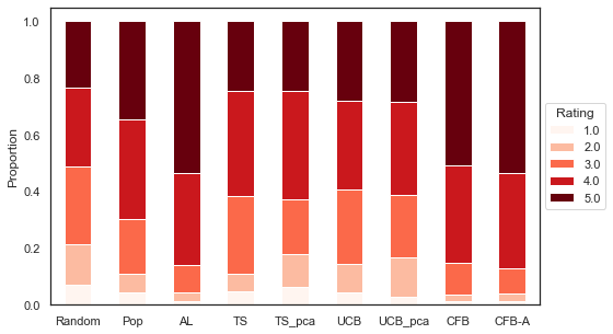
Figure 2: Distribution of Received Ratings by Method (T=120)

Notes: Each color represents the proportion of each categorical rating (1-5) received by recommended movies over T=120. A larger area of a color within a bar implies a higher proportion of its corresponding rating category.

Next we consider the search area dynamics on the bandit stage within the MovieLens data, which investigates the search area of optimal recommendations by each algorithm over time. An algorithm is more efficient if the optimality search is more concentrated over the item space. One advantage of CFB-A is the improved search efficiency, as the bandit stage only needs to search user preferences in a reduced space. Figure 3 shows the boxplots of number of unique items recommended to all 200 new users over three phases when $T=120$. This number decreases as search becomes more efficient (fewer unique items are suggested within the slates of items presented to them).

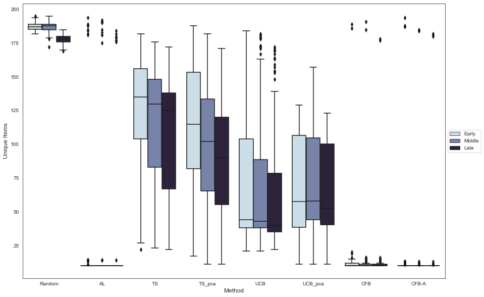
Figure 3: Boxplots of Number of Items Searched (by User and Phase, T=120)

\\\

Notes: Early phase includes periods 61-80; Middle Phase includes periods 81-100; Late Phase includes periods 101-120. The number of unique items for each phase represents the number of non-redundant alternatives recommended to each user in the phase averaged over users. A smaller number implies that less experimentation is needed to infer user preferences and thus less inefficiency in making higher rated recommendations.

The CFB-A and Active Learning, two methods using CFA-solved latent factors, have the highest item concentrations (and therefore the greatest search efficiency) even in early periods when information about consumer preferences is most limited. This implies that CFA-solved latent factors used for data reduction are highly informative for narrowing the search area of bandit learning even at the early stage. Unsurprisingly, the random policy has the most items to explore and therefore the lowest item concentration. Moreover, all traditional bandit approaches have an increasing trend of item concentrations (and of search efficiency) over time, implying a shrinking area of search for the best consumer-item match as they learn. Given TS methods incorporate explorations via sampling which may involve options with higher variances in practice, the TS and TS_pca have lower item concentrations compared to UCB and UCB_pca, respectively. An interesting insight, comparing across methods, is that the cold-start solution generates more search efficiency than the bandit solution, suggesting that the attribute information is relatively informative of user preferences.

4.3 Synthetic Data Simulation

This section first outlines the approach to generate the synthetic data, and then reports the results of our benchmarking analysis.

4.3.1 Data Generation

Recall, the goal of our simulation is to compare how well the various alternative models fare in making recommendations for new users (items) facing a large set of alternatives (users) in contexts with a large number of attributes and demographics. To accomplish this aim, 1000 users are simulated in a market with 1000 items, each characterized by a set of attributes.

Once users and items are created, the next step is to generate the user-item match utility over items. We create two different match utility datasets that vary in how the utility is computed. First, a linear model generates utilities as linear functions of user demographics and item attributes. Second, nonlinear match utilities are constructed where demographics, attributes and utilities are determined using a factor model. The linear model is a standard approach used to construct match utilities in marketing and economics, and the factor model more closely comports to the data reduction approach for specifying match utilities in the CFB-A. Having two different data generating strategies enables an assessment of the robustness of the CFB-A in making recommendations across them.

The linear setting specifies the matrix $Utility\in\mathbb{R}^{I\times J}$ for user $i\in\left\{1,...,I\right\}$ and item $j\in\left\{1,...J\right\}$ as:

$$Utility = \boldsymbol{\beta}\widetilde{A}^{T}+\boldsymbol{\epsilon},$$ (18)

$$\boldsymbol{\beta} = D\Gamma+\boldsymbol{e},$$ (19)

where $D\in\mathbb{R}^{I\times P}$ is the demographic matrix, $\widetilde{A}=\left[\boldsymbol{1}\quad A\right]\in\mathbb{R}^{J\times(Q+1)}$ is the attribute matrix $A$ (appended with a vector of ones to allow for an intercept), and $\boldsymbol{\beta}\in\mathbb{R}^{I\times(Q+1)}$ is the matrix of user preferences for item attributes. Note that these preferences, $\boldsymbol{\beta}$, are a function of user demographics where $\Gamma\in\mathbb{R}^{P\times(Q+1)}$ maps these preferences to demographics, and each element $\Gamma_{pq}$ is i.i.d. $\mathcal{N}(0,1)$. The i.i.d. shocks $\boldsymbol{\epsilon}$ and $\boldsymbol{e}$ are both drawn from a standard normal distribution. The demographic matrix, $D\in\mathbb{R}^{I\times P}$ is constructed by creating a total number of $P=50$ user demographic variables. These demographic variables correspond to indicators for gender, income level, and location. Gender is specified to be a binary variable drawn from a Bernoulli $(p=0.5)$ distribution. In addition, income level for a user is randomly drawn from across one of five categorical levels with equal probability, while location is randomly drawn from across one of 44 categorical locales with equal probability. The attribute matrix, $\widetilde{A}=\left[\boldsymbol{1}\quad A\right]\in\mathbb{R}^{J\times(Q+1)}$ is constructed by creating $Q=300$ categories and randomly assigning items with equal probability to one of those categories or some alternative as reflected by an intercept vector.

In the non-linear setting, the latent spaces and utilities are specified as

$$D=UW^{T},\quad A=V\Psi^{T},$$ (20)

$$Utility=UV^{T}+\boldsymbol{\boldsymbol{\boldsymbol{\varepsilon}}},$$ (21)

where $\left\{U\in\mathbb{R}^{I\times K},V\in\mathbb{R}^{J\times K},W\in\mathbb{R}^{P\times K},\Psi\in\mathbb{R}^{Q\times K}\right\}$ are latent spaces that determine demographics, attributes, and utilities. The number of latent dimensions in the factor space is set to $K=5$. To be consistent with our CFB-A model, all elements in $\left\{U,V,W,\Psi\right\}$ and the random shock $\boldsymbol{\boldsymbol{\varepsilon}}$ are independently drawn from standard normal distributions. As in the linear model, the number of demographic variables is set to $P=50$ and the number of attributes is set to $Q=300$.

After generating the two synthetic datasets, 200 of the 1000 users from each dataset are randomly selected as “new users” to compare the CFB-A against the benchmark models outlined in Section 4.1, and the remaining 800 users from each dataset are regarded as the training set (i.e., existing users). Similar to the MovieLens application, the “existing users” are used to tune the hyper-parameters for each method, including the exploration rate $\alpha$ for methods with a bandit stage, $K$ and $\Sigma$ for CFB-A and Active Learning, $K$ and $\sigma^{2}$ for CFB, and item popularity for the Popularity policy. The total number of periods (rating occasions) over which to generate recommendations is set to $T=15$. Model performance is determined by computing the average cumulative utilities (CAR defined in Equation (17)) across the 200 new users. A higher value of this metric indicates a better recommendation.

4.3.2 Results

Table 4 reports model performance in three representative periods (i.e., the initial, middle, and final periods in the simulated data) and Figure 4 shows the performance by period and simulated data set.

Table 4: Average Cumulative Utilities of Recommended Items by Model and Setting

Technology	Method	Cold Start	Data Reduction		Test and Learn	Utility Type
			Many Users and Items	Many Demographics and Attributes		Linear			Non-Linear
						T=1	T=8	T=15	T=1	T=8	T=15
Null	Random					-0.04	-0.04	-0.06	0	0.01	0
	Popularity					3.87	3.87	3.87	0.10	0.16	0.20
CFA	Active Learning	$\surd$	$\surd$	$\surd$		1.97	1.73	1.71	0.09	0.05	0.05
BA	TS				$\surd$	-0.10	3.14	3.88	0.06	4.80	5.16
	UCB				$\surd$	1.05	4.22	4.61	0	4.85	5.20
	TS_pca			$\surd$	$\surd$	0.02	2.80	3.44	0.04	3.45	3.83
	UCB_pca			$\surd$	$\surd$	0.24	1.26	2.01	-0.16	3.26	3.74
CFB	CFB		$\surd$		$\surd$	1.79	4.54	5.00	0.07	4.90	5.28
CFB-A	CFB-A	$\surd$	$\surd$	$\surd$	$\surd$	5.32	5.80	5.96	5.55	5.67	5.70

Notes: This table reports the average cumulative utilities of items recommended to users by period, utility type, and method. A higher number reflects better recommendations. For example, Thompson sampling generates an average cumulative utility of 3.14 over 8 periods when utilities are generated using the linear method. Utilities generated by the linear simulation range between $\left[-13.64,15.45\right]$ with mean -0.06 and standard deviation 2.10; utilities generated by the non-linear setting range between $\left[-16.71,14.64\right]$ with mean 0 and standard deviation 2.42; a more detailed distributions of utilities in the linear and nonlinear settings can be found in Web Appendix D.

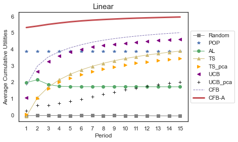
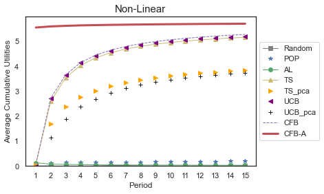
Figure 4: Average Cumulative Utilities of Recommended Items by Model and Period

(a)	(b)

Notes: A period represents a choice occasion, and average cumulative utilities represent the average utilities of recommended alternatives over periods and users. Panel (a) corresponds to the linear setting and Panel (b) corresponds to the non-linear setting.

Four key findings emerge. First, the CFB-A yields the most favorable customer feedback for the recommended items in both the linear and non-linear cases. This suggests the performance enhancement of the CFB-A is robust across various data generating mechanisms. Second, algorithms with the bandit component evidence improved performance over time as a result of learning from feedback. In contrast, approaches without a bandit component (random, popularity, and active learning) do not improve customer responses to their recommendations over time as much. Third, in the linear case, the CFB-A outperforms the second-best approach (POP) in the first period by 37%. Likewise, in the non-linear case, the CFB-A outperforms the second-best approaches (POP) by 5450%. These findings suggest that the CFB-A is effective at addressing cold start. The effect is stronger in the nonlinear case because the underlying data structure aligns with the latent factor model applied by CFB-A, but the finding that performance is enhanced in both cases suggests the robustness of the approach across different data. Fourth, when the data generating process (i.e., linear) differs from the CFB-A model specifications, the initial priors about consumer match are less informative, and therefore the learning stage of CFB-A becomes more important as evidenced by the rapid improvement of CFB-A in initial periods.

5 Live Experiment

Using the MovieLens and simulated data, Section 4 demonstrates that the CFB-A outperforms competing models. While the simulated data are live (i.e., recommendations are updated dynamically) and the MovieLens data are real (i.e., a result of consumers’ rating behaviors), it is desirable to test the CFB-A against competing models in a context that is both live and real. In addition, the CFB-A embeds three key innovations: data reduction, cold-start, and test and learn. Decomposing the relative contribution of each component in terms of improving recommendations would give a sense of their relative import. An experiment accomplishes these twin aims.

5.1 Experimental Context

The Open Science Online Grocery (OSOG) platform, a free research tool established by Howe et al. (2022), is used to conduct an experiment to test the relative performance of the CFB-A in a live setting. The OSOG context affords the engineering infrastructure to implement a recommendation system and allows for many new items and users with many demographics and attributes, making it an appropriate model testing context.

The participant interface mimics e-commerce websites (e.g., Amazon Fresh, Instacart, Walmart), and products on the platform are actual products purveyed at a major grocer in 2018. Upon entering the experimental site via a directed link, participants are presented the category home product listing page (called category home page for short) for the produce category, where they can browse the recommended products in that page, visit another category’s home page, or scroll forward to the second (and beyond) product listing page for the produce category. Figure 5 portrays a subset of products on the produce category’s home page at the online store, as well as the banner menu that can be used to navigate to an alternative category’s home page. Each product listing page, including the category home page and all subsequent product listing pages, includes up to 100 products. The challenge for a recommender system in this context is to determine the order of products presented to a participant on the product listing pages for each category.

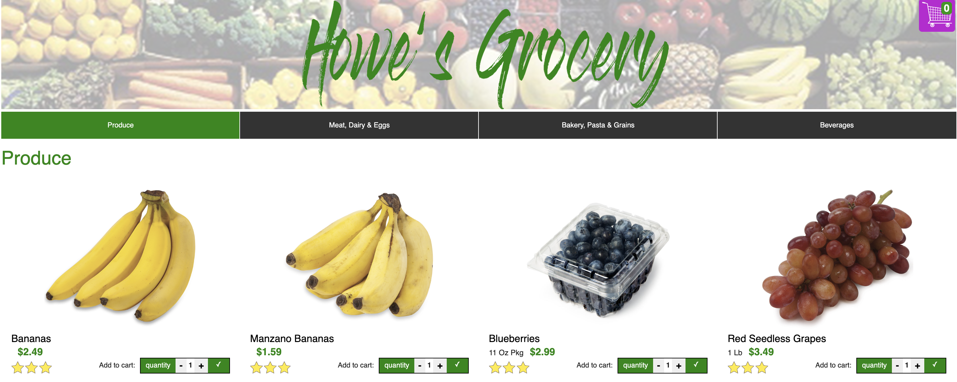
Figure 5: OSOG Product Listing Page

Upon clicking an item on the product listing page, a participant is directed to the product detail page, which displays detailed attribute-level information about the product. An example of the product detail page is shown in Figure 6 for Jarlsberg Swiss Cheese, Lite.

On either the product detail page or product listing page, a participant can add a product to the shopping cart by clicking the product. After adding products to the cart for purchase, the participant can self direct to the checkout page as shown in Figure 7, or continue shopping. Participants end the shopping session by clicking on “Complete Order”.

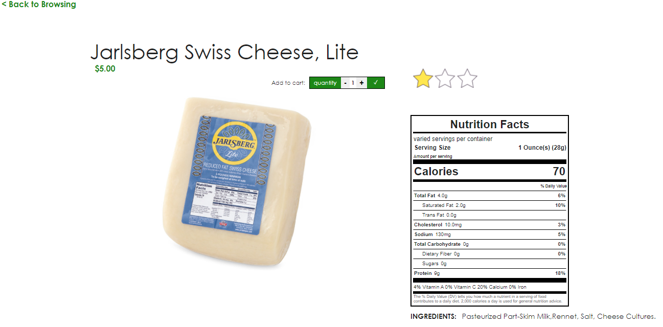
Figure 6: OSOG Product Detail Page

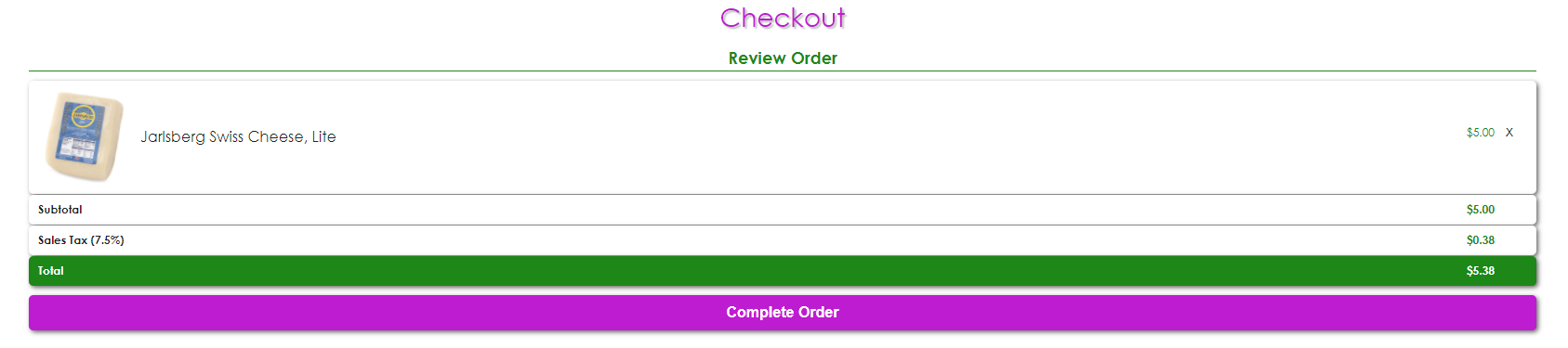
Figure 7: OSOG Checkout Page

The OSOG platform includes 3,542 products across 4 categories: i) produce; ii) meat, dairy, and eggs, iii) bakery, pasta and grains, and iv) beverages. Each product is characterized by multiple attributes, such as price, size, ingredients, nutrition tags (e.g., calories, organic, health starpoints measuring the healthiness of the product, etc.), and allergens. The final attribute space has 22-40 dimensions which vary across categories, as detailed in Web Appendix E.1.

5.2 Experimental Design and Task

5.2.1 Experimental Design

To assess the relative performance of the CFB-A, we compare its performance to three baseline models: the CFB (CF and bandit, no attribute), CFA (CF and attribute, no bandit), and UCB (bandit, no data reduction). This yields four experimental cells. Contrasts between these cells help to highlight the relative importance of the CFB-A innovations: i) the contrast between CFB-A and CFB highlights the role of attributes in improving the cold-start recommendations, ii) the contrast between CFB-A and CFA focuses upon the role of learning in improving recommendations, and iii) the contrast between CFB-A and UCB informs the relative improvement due to the factor space reduction. Notably, these contrasts enable us to decompose the relative benefit of cold start, learning, and dimension reduction to ascertain which is more important for making recommendations in the experimental context.

The experiment consists of two phases, or waves: training and testing. Each phase uses a different set of participants. The one-week training stage, conducted in December of 2021 has two objectives: First, it provides data to “tune” the population-level hyper-parameters in the recommendation systems used in the testing phase, conducted in January and February of 2022. For CFB-A these hyper-parameters include the regularization terms $\Sigma=\left\{\sigma^{2},\sigma_{d}^{2},\sigma_{a}^{2},\lambda_{u},\lambda_{v},\lambda_{w},\lambda_{\psi}\right\}$, the dimension of latent user and product spaces, $K$, and the UCB scale parameter $\alpha$ balancing exploration and exploitation. The hyper-parameters for the other models and the tuning process are detailed in Web Appendix C. In addition, the training stage yields priors for the testing stage, which alleviates the cold-start problem by transforming uninformative priors on latent matrices $W$ and $\Psi$ (which project user or product locations in the latent preference space onto user or product attributes) to informative priors through Equations (12) and (13).

5.2.2 Task

At the beginning of both phases of the experiment, participants complete a survey to elicit their demographics and food preferences (e.g., age, gender, ethnicity, education, household income, household size, state, religion, height, weight, and dietary restrictions). The complete list of collected variables is detailed in Web Appendix E.3 and comprises 119 dimensions. Thus, the demographic data include 119 variables and the product attribute data include 22-40 variables, which should be sufficient to illustrate the improvement of the CFB-A over the CFB. This is likely a conservative test of our model, which can scale readily to larger numbers of attributes and demographics.

After the survey, participants in the training phase completed a single shopping task with a budget of $75 to ensure that they do not select an inordinately large number of products. The order of products presented to each participant in the training phase was randomized within each category. Participants made product selection decisions by adding products to cart, and were free to revisit prior detail and listing pages before the checkout decision. To avoid potential inventory effect suppressing choices of preferred products, participants were requested to imagine they had no grocery at home when completing the shopping task. The final participant decision was to end the shopping visit, at which point the experimental session ends.

Participants in the testing phase were asked to revisit the experiment one- , two- , and three-weeks after the demographic survey in the first week, and complete a shopping task with a budget of $75 in each visit. As with the training phase, participants’ clicks on products and purchases are recorded. Unlike the training phase where product order is randomized, the order of products presented to participants in the second week of the testing phase (i.e., one week after the demographic survey was administered) was determined by the algorithm for the given experimental cell based on reported demographics and participant purchases in the training phase. The order of products presented in the third and the fourth weeks of the testing phase further considers participant purchases in the preceding weeks of the testing phase.

5.3 Subjects

Two waves of participants were recruited via CloudResearch, corresponding to the two experimental phases: training and testing. In total, 531 subjects participated in the training phase and 847 subjects participated in the testing phase. Participants in the testing phase were randomly assigned to one of the four experimental cells. The participants were largely representative of the United States with respect to age, gender, and ethnicity on Mturk, as directed by the CloudResearch recruitment settings. Participants were compensated $0.12/minute and those in the testing phase received a bonus of $1 for completing all four sessions. On average, participants spent 16.7 minutes completing a survey with the shopping task. In addition, attention checks were used to ensure data quality, and 1.1% of participants failing to pass these checks did not receive compensation (details on these checks are provided in Web Appendix E.2).

5.4 Performance Metric

Model performance is evaluated via homepage (the category home product listing page) purchase rates (HPR) of each category, which captures participants’ tendency to purchase the 100 most highly recommended products. HPR is an ideal performance metric for several reasons. First, all participants browsed the home page, whereas many fewer of them (from 45% to 73% depending on the category) browsed any listing page beyond the home page. Thus the HPR metric is not affected by products a participant does not typically see. Second, by focusing on a specific set size of products, the metric is comparable in interpretation across categories relative to one that uses different set sizes. Third, the homepage performance is also of practical business interest because the homepage sales rates are a KPI of interest and because including less relevant products on the home page can induce customer churn.

The HPR for category $c$ in period $t$ is computed as follows:

$$HPR_{t}^{c} = \frac{1}{I\times J}\sum_{i=1}^{I}\sum_{j=1}^{J}Purchases_{ijt}^{c},$$ (22)

where $i$ denotes participant and $j$ denotes product, $J=100$ is the total number of products on the home page. $Purchases_{ijt}^{c}$ is an indicator variable which takes the value of 1 if participant $i$ purchased product $j$ in period $t$. The period-level purchase rate can be extended to a cumulative (over all the shopping periods thus far) purchase rate for category $c$ in period $t$ as follows:

$$cHPR_{t}^{c}=\frac{1}{t}\sum_{\tau=1}^{t}HPR_{\tau}^{c}$$ (23)

The category-level HPR and cumulative HPR can be aggregated to a site-level HPR measure by averaging or summing across the four categories.

5.5 Results

Using the HPR metric described in Section 5.4, this section compares model performance across the experimental cells (corresponding to the four methods outlined in Section 5.2.1), and decomposes the relative contributions of data reduction, cold-start, and test and learn. We first report results aggregated across all categories and then detail the category-specific results to assess conditions under which any one of the three components (data reduction, cold-start, and test and learn) contributes most in the CFB-A.

5.5.1 Aggregate Site-Level Results

Figure 8 depicts the cumulative HPR (cHPR), for each method and period across all categories in the experiment. Asterisks indicate the statistical significance of the difference between the CFB-A and the respective benchmark model as determined by independent two-sample t-tests. The cHPRs of CFB-A, CFA, CFB, and UCB at the conclusion of the experiment (period 3) are respectively 3.91%, 3.63%, 3.29%, and 2.32%. The CFB-A significantly outperforms the three benchmark models. In percentage terms, the CFB-A outperforms the UCB by 69%, (contribution due to data reduction), the CFB by 19% (contribution due to cold start), and the CFA by 8% (contribution due to test and learn). Compared to the worst performing model, the CFB-A nearly doubles the cHPR. The larger improvement of CFB-A over CFB relative to CFA implies that A (cold start) matters more than B (test and learn), presumably due to informative priors (that is, demographics and attributes can predict choices). However, the comparative advantages of A and B can be context-dependent, which motivates us to compare the performance of these methods for each category.

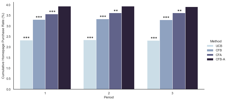
Figure 8: cHPR Combined Over Categories By Period

Notes: Period represents week, or choice occasion, in the experiment. Each bar represents the cHPR for a given method and period. For example, the CFB-A yields a cHPR of 3.91% in period 3 as evidenced by the last bar. Independent two-sample t-tests compare the cHPRs under CFB-A and each benchmark method, and the t-values for the contrasts between methods are reported in Web Appendix E.5. Significance levels are denoted as follows: $**p<.05,***p<.01$.

The increased HPR translates to increased homepage retailer sales. In particular, the CFB-A generates an average of $52.39 in homepage sales per subject, while the CFB, CFA, and UCB generate an average homepage sales of $50.14, $50.79, and $32.87 respectively. According to the one-sided independent two-sample t-test, the increase in CFB-A sales relative to the other approaches are all statistically significant or marginally significant (with t-values as follows: CFB-A vs CFB ($t=1.47$), CFB-A vs CFA ($t=1.74$), and CFB-A vs UCB ($t=17.00$)).

To obtain a deeper insight into how the CFB-A recommendation algorithm affects total consumer demand at the grocery site, we compare the total number of products purchased and total revenue across all sessions and pages within the session (i.e., not just the home pages). The number of products sold under CFB-A is significantly or marginally significantly higher than under CFB and UCB (the t-values for the independent two-sample t-tests are as follows: CFB-A vs CFB (22.7 vs 19.7, $t=4.31$), CFB-A vs CFA (22.7 vs 22.0, $t=0.93$), and CFB-A vs UCB (22.7 vs 21.6, $t=1.39$)). However, there is little difference in total site revenue across the four benchmark methods (the t-values for the independent two-sample t-tests as follows: CFB-A vs CFB ($64.72 vs $64.92, $t=\text{\textendash}0.13$), CFB-A vs CFA ($64.72 vs $64.29, $t=0.26$), and CFB-A vs UCB ($64.72 vs $64.22, $t=0.31$)). Given that more products are sold under CFB-A, but there is no difference in revenue, it follows that lower priced products, on average are sold under CFB-A. The average price of products on the home page under CFB-A is significantly lower than under CFB and CFA (the t-values for the independent two-sample t-tests are as follows: CFB-A vs CFB ($3.61 vs $3.82, $t=-22.58$), CFB-A vs CFA ($3.61 vs $3.72, $t=-11.24$), and CFB-A vs UCB ($3.61 vs $3.62, $t=-0.36$)). The finding that the CFB-A serves the lowest prices suggests that it tends to capture user preferences for lower prices better than the other algorithms.

In sum, the CFB-A yields two key implications for the experimental site. First, as implied by the increase in the cHPR performance metric, which focuses on purchases within the first 100 products, the CFB-A recommends preferred products earlier in the ordered set of available products relative to the other extant methods (i.e., the first 100 products contain more consumer matches). This result is also consistent with the finding that the CFB-A outperforms other methods under the NDCG metric (Järvelin and Kekäläinen, 2002), which accounts for product rank and favors recommendation engines that place chosen products earlier in the list. Second, because more products are sold in the experimental grocery site while the grocer’s revenue remains constant, the CFB-A tends to recommend less expensive products, which could limit the revenue implications of the recommender system in retail settings.

We make several observations about these two implications. First, the effect of price on revenue is a concern relatively unique to retail. In settings without variable item prices, such as online news (which is monetized by viewership) or movie recommendations and OTAs (where prices or referral fees tend to be constant with clicks), sites are unambiguously better off with higher cHPR because monetization increases with items viewed or ordered. Second, the current experiment uses cHPR as the performance measure in hyper-parameter tuning, and CFB-A is likely to lead to higher revenue if renenue were used as the performance measure. Third, even if actual site revenues were constant in practice upon adopting the CFB-A, the finding that consumers obtained higher utility from goods purchased indicates that the retailer is better off because satisfied customers are less likely to attrite.

5.5.2 Category-level Results

Figure 9 portrays the cHPR of the CFB-A and the three benchmark models at the conclusion of the experiment (period 3) by product category. Consistent with the aggregate results, a comparison between CFB-A and UCB indicates that data reduction yields the largest gains in cHPR for each category. Notably, a comparison of CFB-A and CFB indicates that cold start has the most salient role in the category of meat, dairy, and eggs, while a comparison of CFB-A and CFA indicates that test and learn only makes a difference in produce.

Figure 9: Period 3 cHPR by Category

\\\\

Notes: Each bar represents the cHPR for a given method and category over all periods in the experiment. Specific cHPR values for each category and method are reported in Web Appendix E.5. Independent two-sample t-tests compare the cHPR under CFB-A and each benchmark method, and the t-values for these method contrasts can be found in Web Appendix E.5. Significance levels are denoted as follows: $*p<.10,***p<.01$.

The differences of the relative importance of A (cold start) across categories imply that the informativeness of attributes on preferences differs across categories. The A part (cold start) is expected to be more important than the B part (test and learn) when attributes are perfectly informative about preferences. If attributes perfectly predict preferences, there is nothing to learn. As attributes become less predictive, there is, in general, increasing value in B.

Assessing the role of the informativeness of attributes on preferences requires a metric of informativeness. One such metric is available from the one-period training data, which is based on the counterfactual HPRs for the CFA and CF models (note there is no B component as the training data consist of only one period). Specifically, the percentage HPR lift in the training data for the counterfactual CFA relative to the counterfactual CF measures how well attributes explain outcomes (i.e., how much the attribute information matters). In other words, when the CFA improves over the CF on the training sample, the quality of priors embedding attributes is higher for predicting initial preferences and making initial recommendations.

Table 5 reports, by category, both the informativeness of attributes (by quality of prior) in the training data (column 2) and the relative contribution of A to B in the testing data (columns 3 to 5). The correlation between the second column ($Gain_{A,Train}$) and the last column ($Gain_{A}/Gain_{B}$) across the four categories is 0.83 and there is a monotonic relation between the entries in the two columns. Therefore, the relative importance of A to B in the testing data increases as A becomes more informative in the training data, as we have conjectured. In other words, as attributes become increasingly informative of preferences, the cold-start component of the model (A) becomes relatively more useful for recommendations than the test-and-learn component (B) of the model.

Table 5: The Effect of Attribute Salience on the Relative Contribution of A

Category	Training Data		Testing Data
	$Gain_{A,Train}=\frac{HPR_{CFA}-HPR_{CF}}{HPR_{CF}}$		$Gain_{A}=\frac{cHPR_{CFB-A}-cHPR_{CFB}}{cHPR_{CFB-A}}$	$Gain_{B}=\frac{cHPR_{CFB-A}-cHPR_{CFA}}{cHPR_{CFB-A}}$	$\frac{Gain_{A}}{Gain_{B}}$
Meat, Dairy, and Eggs	469%		21%	2%	10.5
Produce	318%		9%	12%	0.8
Beverages	232%		5%	–11%	–0.5
Bakery, Pasta, and Grains	12%		4%	–3%	–1.3

Notes: The first column reports the category, the second column reports the percentage increase in the HPR for the CFA relative to CF in the training data, the third column reports the increase in the cHPR for the CFB-A relative to the CFB (normalized by the cHPR under CFB-A and representing the gain from A), the fourth column reports the increase in the cHPR for the CFB-A relative to the CFA (normalized by the cHPR under CFB-A and representing the gain from B), and the final column reports the ratio of the gain from A reported in the third column to the gain from B reported in the fourth column (in other words, the last column is a measure of relative importance of A to B in improving forecasts). Please see Table A.1 in Web Appendix E.5 for values used in the testing data computations; for example in produce $Gain_{A}=(7.19-6.53)/7.19=9\%$.

In summary, our results provide three main takeaways. First, CFB-A has the best aggregate performance. Second, given that UCB has the worst performance throughout, data reduction has the largest contribution. Third, the relative importance of cold start and test and learn is context-dependent: though the CFB-A tends to perform better when A explains consumer choices, the test and learn component can perform better when attributes are moderately informative of preferences, because the bandit can better ascertain the dimensions along which consumer preferences are uncertain (when A is entirely uninformative, all error variances are high and B has a harder time assessing where to explore).

6 Conclusion

This paper considers recommendation systems common in many digital contexts such as news, music, shopping, or streaming where new users and new items are common, the space of users and items is large, and the tags used to describe them are extensive. In such contexts, collaborative filtering exhibits cold-start limitations as there is little history upon which to base recommendations.

We develop a model specifically for these contexts that embeds two key components. One component reduces the dimensionality of recommender data, and thus enables the approach to scale to larger applications. Specifically, this component factors the user-by-item preference matrix, the user-by-demographic matrix, and the item-by-attribute matrix. One key benefit of this factorization is the ability to address the cold-start problem by recommending items preferred by others who are similar in their demographic composition (denoted as the CFA). A second component involves a bandit approach to test and learn them (denoted as the CFB), and this becomes more relevant when demographics are not sufficiently informative about user preferences. A key advance is to combine the CFA and CFB into the CFB-A. One notable synergy arising from this combination is that the bandit needs only search for items in a much reduced space. Hence it scales well. A second notable synergy is that the recommendation approach becomes more robust. When observables such as demographics are predictive of preferences, our model uses this information to make better predictions. When unobservables are less informative, our model uses bandit exploration on past choices to improve recommendations. In this sense, combining the two components leads to a more robust recommendation approach.

As a result, the combination of the two components (CFA and CFB) into a CFB-A yields material gains in the quality of consumer recommendations in the context of collaborative filtering (CF). The model is benchmarked against a wide array of extant alternatives that address scale, cold-start, or bandit learning but not all three. We do so using standard benchmarking data from MovieLens, a simulation, and a grocery experiment. In sum, we benchmark over a large set of models (that contain components of our innovations) and datasets (static, simulated, and live).

In each case, the CFB-A improves upon the alternative models, and the degree of improvement varies across models and data sets (compared to the next best approach for each data set, CFB-A improves by about 1% in the MovieLens data, 19% in the synthetic data, and 8% in the experimental data). In general, when attributes are informative about preferences and feedback scales are informative, our model works better than those that omit attributes. When attributes are less informative, our model works better than those that omit the bandit. Moreover, our model converges more quickly to the best option than other approaches, because the bandit can learn user preferences more quickly in the reduced user (item)-attribute spaces (in one case, user preferences are learned in one to two recommendations whereas other approaches require closer to ten). The empirical performance of the CFB-A suggests future theoretical work on the regret bounds and convergence rate of this method to formalize the mechanisms underpinning its advantages in combining CF, B, and A.

The utility of our analysis is of straightforward benefit to practitioners. Those facing issues of scale and cold start in recommender contexts stand to gain directly from our algorithm. Our research may have policy implications for an increasingly privacy-oriented environment. By balancing learning from first-party data with demographics from first- and third-party data, our approach is relatively robust to changes in the data environment. It is even possible for third-party firms to compute user factor “scores” to assure privacy on given covariates, as the factors scores by themselves are not sufficient to impute demographics that underpin them (as scores are a linear combination of demographics). In other words, scores are more privacy compliant than demographics and would still enable better cold-start recommendations.

Beyond these immediate applications, a set of broader questions of relevance to our research exist. First, though the algorithm scales well, it requires updating based on past choices. Given the engineering challenges of updating item positions in a real-time environment, assessing the optimal level of updating (such as real time, minute, hour, or daily frequency) or how to batch recommendations is of interest. Second, hybrid recommendation methods have recently combined state-of-the-art representation learning techniques (e.g., autoencoders) with traditional heuristics (e.g., matrix factorization, logistic regression) (Jannach et al., 2020; Strub et al., 2016; Dong et al., 2020; Geng et al., 2022; Zhou et al., 2023), suggesting that CFB-A could be improved by combining matrix factorization with autoencoders. In addition, other inference techniques, such as variational inference (Ansari et al., 2018), can be used as an alternative to MCMC estimation for the Bayesian component of CFB-A. Related and third, ours is a list recommender system. It is relatively straightforward to extend the approach to menu recommendations by modeling user preference for one item to be a function of all recommended items. This extension would be an interesting new direction which captures complementarity and substitutability between items (e.g., Kumar et al., 2020a). Fourth, while CFB-A improves the cumulative direct rewards such as clicks, purchases, and ratings, it would be of interest to assess how recommendation approaches affect indirect outcomes such as consumer loyalty in the long run. Fifth, as the CFB-A combines both aggregate preference information and user choices, a pertinent question is whether it can mitigate tendencies to be polarizing or homogenizing (e.g., Hosanagar et al., 2014; Lee and Hosanagar, 2019; Berman and Katona, 2020; Su et al., 2016; Zhang et al., 2022) and how it can be used to enhance diversity (e.g., Song et al., 2019; Zhou et al., 2023). Finally, in any recommendation system, algorithmic bias (e.g., Cowgill and Tucker, 2019) is a concern. Owing to its flexibility in combining information from own and others’ choices as well as item attributes and consumer characteristics, the potential for the CFB-A to ameliorate algorithmic bias is a worthwhile future direction. It is promising that the test-and-learn component can enhance recommendation performance in the absence of third-party data used in cold start (such as racial demographics), making the CFB-A more robust in capturing preferences. We hope others will build on the ideas in this paper to address these and other timely and relevant issues in the context of recommendation systems.

Funding and Competing Interests

All authors certify that they have no affiliations with or involvement in any organization or entity with any financial interest or non-financial interest in the subject matter or materials discussed in this manuscript. The authors have no funding to report.

Appendix

Appendix A Model Notation

Table A.1 details the notational definitions used throughout the paper.

Table A.1: Notation

Notation	Definition
For CFA (§3.2)
$K$	The dimension of latent representation space determined by CF
$I$	The number of users
$J$	The number of items
$P$	The dimension of user feature vector
$Q$	The dimension of item feature vector
$D$, $A$	Matrices of user demographics and item attributes, respectively
$\mu_{ij}$	The mean feedback of user $i$ to item $j$ (e.g. rankings, choices, etc.)
$y_{ij}$	An indicator which equals to 1 if feedback of user $i$ to item $j$ is observed, and 0 otherwise
$U=\left[\boldsymbol{u}_{1},\boldsymbol{u}_{2},\cdots,\boldsymbol{u}_{I}\right]^{T}$	Latent representations for user location in preference space
$V=\left[\boldsymbol{v}_{1},\boldsymbol{v}_{2},\cdots,\boldsymbol{v}_{J}\right]$	Latent representation for item location in preference space
$W=\left[\boldsymbol{w}_{1},\boldsymbol{w}_{2,}\cdots,\boldsymbol{w}_{P}\right]$	Matrix projecting user locations in the latent preference space onto user demographics
$\Psi=\left[\boldsymbol{\psi}_{1},\boldsymbol{\psi}_{2},\cdots,\boldsymbol{\psi}_{Q}\right]$	Matrix projecting item locations in the latent preference space onto item attributes
$\Sigma=\{\sigma^{2},\sigma_{d}^{2},\sigma_{a}^{2},\lambda_{u},\lambda_{v},\lambda_{w},\lambda_{\psi}\}$	CFA hyper-parameters
$\overline{\boldsymbol{v}},\overline{\boldsymbol{u}},\overline{\boldsymbol{w}},\overline{\boldsymbol{\psi}},\Sigma_{v},\Sigma_{u},\Sigma_{w},\Sigma_{\psi}$	Posterior means and covariances of $U,V,W,\Psi$, respectively
For Bandit Learning (§3.3)
$T$	The total number of feedback occasions
$CAR$	The expected cumulative rewards at time $t$
For Experiments (§4 and §5)
$\Gamma$	Matrix projecting preferences to demographics in the linear setting
$\boldsymbol{\epsilon}$, $\boldsymbol{e}$, $\boldsymbol{\boldsymbol{\varepsilon}}$	Random iid normal errors
$HPR_{t}^{c}$	Purchase rate on the home page of category $c$ in period $t$
Throughout the Paper
*	A superscribe to remark the optimal solutions of the corresponding variable
$\widehat{}$	A symbol to remark the estimate of the corresponding variable

Appendix B The CFB-A Algorithm

Algorithms 1 (for UCB) and 2 (for TS) outline the CFB-A algorithms for learning either new users’ preferences on existing items or for learning existing users’ preferences on new items. We exemplify the algorithm with the case of new users.

Algorithm 1 CFB-A (UCB)

Pre-determined hyper-parameters: $K,\sigma^{2},\sigma_{d}^{2},\lambda_{u},\lambda_{w},\alpha$

Observed variables: $\mu_{ij,t}$ for user $i$, item $j$, and user demographics $\boldsymbol{d}_{i,t}$ at time $t$

Variables pre-computed with existing users and items (training set): CFA-estimated item latent factors $\boldsymbol{v}$ and user demographic latent factors $\boldsymbol{w}_{0}$

Initialization of regularization parameters and priors: $S\leftarrow\lambda_{u}\sigma^{2}I_{K};\boldsymbol{b}\leftarrow S(\boldsymbol{d}_{i,0}^{T}\boldsymbol{w}_{0}^{g})^{T};S_{u}\leftarrow\lambda_{w}\sigma_{d}^{2}I_{K};\boldsymbol{b}_{u}\leftarrow S_{u}\boldsymbol{w}_{0}$

for $t=1,2,...,T$

Calculate $\boldsymbol{w}_{t}=S_{u}^{-1}\boldsymbol{b}_{u};\boldsymbol{u}_{i,t}=S^{-1}\boldsymbol{b};\Sigma_{i,t}=S^{-1}\sigma^{2}$ (CFA estimation)

Select the item $j^{*}=\arg\max_{j}\left(\boldsymbol{u}_{i,t}^{T}\boldsymbol{v}_{j}+\alpha_{t}\cdot\sqrt{\boldsymbol{v}_{j}^{T}\Sigma_{i,t}\boldsymbol{v}_{j}}\right)$ for each user $i$ (UCB Bandit allocation)

Observe user feedback to recommended items $\overrightarrow{\mu}_{ij^{*}t}$, and incorporate newly observed user demographics $\boldsymbol{d}_{i,t}$

Update $S_{u}\leftarrow S_{u}+\mathbb{I}\left[i\thinspace makes\thinspace any\thinspace choices\right]\cdot\boldsymbol{u}_{i,t}\boldsymbol{u}_{i,t}^{T}$ (CFA estimation)

$\boldsymbol{b}_{u}\leftarrow\boldsymbol{b}_{u}+\mathbb{I}\left[i\thinspace chooses\thinspace j^{*}\right]\cdot\boldsymbol{u}_{i,t}\boldsymbol{d}_{i,t}^{T}$(CFA estimation)

$S\leftarrow S+\mathbb{I}\left[i\thinspace chooses\thinspace j^{*}\right]\cdot\boldsymbol{v}_{j^{*}}\boldsymbol{v}_{j^{*}}^{T}+\frac{\sigma^{2}}{\sigma_{d}^{2}}\boldsymbol{w}_{t}\boldsymbol{w}_{t}^{T}$ (CFA estimation)

$\boldsymbol{b}\leftarrow\boldsymbol{b}+\mathbb{I}\left[i\thinspace chooses\thinspace j^{*}\right]\cdot\boldsymbol{v}_{j^{*}}\cdot\mu_{ij^{*}}+\frac{\sigma^{2}}{\sigma_{d}^{2}}\boldsymbol{w}_{t}\boldsymbol{d}_{i,t}^{T}$ (CFA estimation)

$t\leftarrow t+1$

end for

Notes: rate $\alpha_{t}$ is a slowly increasing function of $t$ to maintain exploration as uncertainties $\sqrt{\boldsymbol{v}_{j}^{T}\Sigma_{i,t}\boldsymbol{v}_{j}}$ decrease over time (Zhao et al., 2013; Filippi et al., 2010). $\alpha_{t}$ is specified as $\alpha\sqrt{\log t}$ and $\alpha\sqrt{t}$ in practice.

Algorithm 2 CFB-A (TS)

Pre-determined hyper-parameters: $K,\sigma^{2},\sigma_{d}^{2},\lambda_{u},\lambda_{w}$

Observed variables: $\mu_{ij,t}$ for user $i$, item $j$, and user demographics $\boldsymbol{d}_{i,t}$ at time $t$

Variables pre-computed with existing users and items (training set): CFA-estimated distributions of item latent space $\mathcal{F}_{V}$ (item $j$ has $\boldsymbol{v}_{j}$ randomly drawn from $\mathcal{N}\left(\overline{\boldsymbol{v}}_{j},\Sigma_{\boldsymbol{v}_{j}}\right)$) and user demographic latent space $\mathcal{F}_{W}^{0}$ (priors, demographic features $\boldsymbol{w}_{0}$ are randomly drawn from $\mathcal{N}\left(\overline{\boldsymbol{w}}_{0},\Sigma_{0}^{w}\right)$).

Initialization of regularization parameters and priors: $S\leftarrow\lambda_{u}\sigma^{2}I_{K};\boldsymbol{b}\leftarrow S(\boldsymbol{d}_{i,0}^{T}\boldsymbol{w}_{0}^{g})^{T};S_{u}\leftarrow\lambda_{w}\sigma_{d}^{2}I_{K};\boldsymbol{b}_{u}\leftarrow S_{u}\boldsymbol{w}_{0}$

for $t=1,2,...,T$

Calculate $\overline{\boldsymbol{w}}_{t}=S_{u}^{-1}\boldsymbol{b}_{u};\text{$\Sigma_{t}^{w}=$$S_{u}^{-1}$$\sigma_{d}^{2}$};\overline{\boldsymbol{u}}_{i,t}=S^{-1}\boldsymbol{b};\Sigma_{i,t}=S^{-1}\sigma^{2}$ (CFA estimation)

Select the item $j^{*}=\arg\max_{j}\boldsymbol{u}_{i,t}^{T}\boldsymbol{v}_{j}$ for each user $i$, where $\boldsymbol{u}_{i,t}$ is randomly drawn from $\mathcal{N}\left(\overline{\boldsymbol{u}}_{i,t},\Sigma_{i,t}\right)$ (TS Bandit allocation)

Observe user feedback to recommended items $\overrightarrow{\mu}_{ij^{*}t}$, and incorporate newly observed user demographics $\boldsymbol{d}_{i,t}$

Update $S_{u}\leftarrow S_{u}+\mathbb{I}\left[i\thinspace makes\thinspace any\thinspace choices\right]\cdot\boldsymbol{u}_{i,t}\boldsymbol{u}_{i,t}^{T}$ (CFA estimation)

$\boldsymbol{b}_{u}\leftarrow\boldsymbol{b}_{u}+\mathbb{I}\left[i\thinspace chooses\thinspace j^{*}\right]\cdot\boldsymbol{u}_{i,t}\boldsymbol{d}_{i,t}^{T}$(CFA estimation)

$S\leftarrow S+\mathbb{I}\left[i\thinspace chooses\thinspace j^{*}\right]\cdot\boldsymbol{v}_{j^{*}}\boldsymbol{v}_{j^{*}}^{T}+\frac{\sigma^{2}}{\sigma_{d}^{2}}\boldsymbol{w}_{t}\boldsymbol{w}_{t}^{T}$, where $\boldsymbol{w}_{t}$ is randomly drawn from $\mathcal{N}\left(\overline{\boldsymbol{w}}_{t},\Sigma_{t}^{w}\right)$ (CFA estimation)

$\boldsymbol{b}\leftarrow\boldsymbol{b}+\mathbb{I}\left[i\thinspace chooses\thinspace j^{*}\right]\cdot\boldsymbol{v}_{j^{*}}\cdot\mu_{ij^{*}}+\frac{\sigma^{2}}{\sigma_{d}^{2}}\boldsymbol{w}_{t}\boldsymbol{d}_{i,t}^{T}$ (CFA estimation)

$t\leftarrow t+1$

end for

Web Appendix

Appendix A Posterior Distributions for $U,V$ in the CF Model

The likelihood of preference $\boldsymbol{\mu}$ over users and items given $U$, $V$ and hyper-parameters is:

$$P\left(\boldsymbol{\mu}\mid U,V,\lambda_{u},\lambda_{v},\sigma^{2}\right)=\Pi_{i=1}^{I}\Pi_{j=1}^{J}\left[\mathcal{N}\left(\mu_{ij}\mid\boldsymbol{u}_{i}^{T}\boldsymbol{v}_{j},\lambda_{u},\lambda_{v},\sigma^{2}\right)\right]^{y_{ij}}$$ (1)

A.1 Posterior of $U$

The posterior of $U$ is as follows:

$$p\left(U\mid\boldsymbol{\mu},V,\lambda_{u},\lambda_{v},\sigma^{2}\right) \propto p\left(\boldsymbol{\mu}\mid U,V,\lambda_{u},\lambda_{v},\sigma^{2}\right)\cdot p\left(U\mid\lambda_{u},\lambda_{v},\sigma^{2}\right)$$

$$\propto \Pi_{i=1}^{I}\mathcal{N}\left(\boldsymbol{u}_{i}\mid\textbf{0},\sigma_{u}^{2}\mathbf{I}_{K}\right)\cdot$$

$$\Pi_{i=1}^{I}\Pi_{j=1}^{J}\left[\mathcal{N}\left(\mu_{ij}\mid U,V,\lambda_{u},\lambda_{v},\sigma^{2}\right)\right]^{y_{ij}=1}\cdot$$

$$\propto \Pi_{i=1}^{I}\exp\left\{-\frac{1}{2}\lambda_{u}\boldsymbol{u}_{i}^{T}\boldsymbol{u}_{i}-\frac{1}{2}\left[\frac{1}{\sigma^{2}}\sum_{y_{ij}=1}\left(\mu_{ij}-\boldsymbol{u}_{i}^{T}\boldsymbol{v}_{j}\right)^{2}\right]\right\}$$

$$\propto \Pi_{i=1}^{I}\exp\left\{-\frac{1}{2}\left[\boldsymbol{u}_{i}^{T}\left(\lambda_{u}\mathbf{I}_{K}+\frac{1}{\sigma^{2}}\sum_{y_{ij}=1}\boldsymbol{v}_{j}\boldsymbol{v}_{j}^{T}\right)\boldsymbol{u}_{i}-2\frac{1}{\sigma^{2}}\sum_{y_{ij}=1}\mu_{ij}\boldsymbol{u}_{i}^{T}\boldsymbol{v}_{j}\right]\right\}$$

$$\propto \Pi_{i=1}^{I}\mathcal{N}\left(\boldsymbol{u}_{i}\mid\overline{\boldsymbol{u}}_{i},\Sigma_{\boldsymbol{u}_{i}}\right)$$

Thus, $\boldsymbol{u}_{i}\sim\mathcal{N}\left(\overline{\boldsymbol{u}}_{i},\Sigma_{\boldsymbol{u}_{i}}\right)$, where

$$\overline{\boldsymbol{u}}_{i}=\left(\frac{1}{\sigma^{2}}\sum_{j}y_{ij}\cdot\mu_{ij}\boldsymbol{v}_{j}\right)\Sigma_{\boldsymbol{u}_{i}},$$ (3)

$$\Sigma_{\boldsymbol{u}_{i}}=\left(\lambda_{u}\mathbf{I}_{K}+\sum_{j}y_{ij}\cdot\frac{1}{\sigma^{2}}\boldsymbol{v}_{j}\boldsymbol{v}_{j}^{T}\right)^{-1}$$ (4)

A.2 Posterior of $V$

The posterior of $V$ is as follows:

$$p\left(V\mid\boldsymbol{\mu},U,\lambda_{u},\lambda_{v},\sigma^{2}\right) \propto p\left(\boldsymbol{\mu}\mid U,V,\lambda_{u},\lambda_{v},\sigma^{2}\right)\cdot p\left(V\mid\lambda_{u},\lambda_{v},\sigma^{2}\right)$$

$$\propto \Pi_{j=1}^{J}\mathcal{N}\left(\boldsymbol{v}_{j}\mid\textbf{0},\lambda_{v}^{-1}\mathbf{I}_{K}\right)\cdot$$

$$\Pi_{i=1}^{I}\Pi_{j=1}^{J}\left[\mathcal{N}(\mu_{ij}\mid U,V,\lambda_{u},\lambda_{v},\sigma^{2})\right]^{y_{ij}=1}\cdot$$

$$\propto \Pi_{j=1}^{J}\exp\left\{-\frac{1}{2}\lambda_{v}\boldsymbol{v}_{j}^{T}\boldsymbol{v}_{j}-\frac{1}{2}\left[\frac{1}{\sigma^{2}}\sum_{y_{ij}=1}\left(\mu_{ij}-\boldsymbol{u}_{i}^{T}\boldsymbol{v}_{j}\right)^{2}\right]\right\}$$

$$\propto \Pi_{j=1}^{J}\exp\left\{-\frac{1}{2}\left[\boldsymbol{v}_{j}^{T}\left(\lambda_{v}\mathbf{I}_{K}+\frac{1}{\sigma^{2}}\sum_{y_{ij}=1}\boldsymbol{u}_{i}\boldsymbol{u}_{i}^{T}\right)\boldsymbol{v}_{j}-2\frac{1}{\sigma^{2}}\sum_{y_{ij}=1}\mu_{ij}\boldsymbol{v}_{j}^{T}\boldsymbol{u}_{i}\right]\right\}$$

$$\propto \Pi_{j=1}^{J}\mathcal{N}\left(\boldsymbol{v}_{j}\mid\overline{\boldsymbol{v}}_{j},\Sigma_{\boldsymbol{v}_{j}}\right)$$

Thus, $\boldsymbol{v}_{j}\sim\mathcal{N}\left(\overline{\boldsymbol{v}}_{j},\Sigma_{\boldsymbol{v}_{j}}\right)$, where

$$\overline{\boldsymbol{v}}_{j}=\left(\frac{1}{\sigma^{2}}\sum_{i}y_{ij}\cdot\mu_{ij}\boldsymbol{u}_{i}\right)\Sigma_{\boldsymbol{v}_{j}}$$ (6)

$$\Sigma_{\boldsymbol{v}_{j}}=\left(\lambda_{v}\mathbf{I}_{K}+\sum_{i}y_{ij}\cdot\frac{1}{\sigma^{2}}\boldsymbol{u}_{i}\boldsymbol{u}_{i}^{T}\right)^{-1}$$ (7)

Appendix B Posterior Distributions for $U,V,W,\Psi$ in the CFA Model

The joint likelihood of $\left\{\boldsymbol{\mu},D,A\right\}$ over users and items given latent spaces $\left\{U,V,W,\Psi\right\}$ and hyper-parameters is:

$$P\left(\boldsymbol{\mu},D,A\mid U,V,W,\Psi,\Sigma\right) = P\left(\boldsymbol{\mu}\mid D,A,U,V,W,\Psi,\Sigma\right)P\left(D,A\mid U,V,W,\Psi,\Sigma\right)$$

$$= \Pi_{i=1}^{I}\Pi_{j=1}^{J}\left[\mathcal{N}(\mu_{ij}\mid\boldsymbol{a}_{j},\boldsymbol{d}_{i},U,V,W,\Psi,\Sigma)\right]^{y_{ij}=1}\cdot$$

$$\Pi_{p=1}^{P}\mathcal{N}(d_{ip}\mid U,W,\Sigma)\Pi_{q=1}^{Q}\mathcal{N}(a_{jq}\mid V,\Psi,\Sigma)$$

where $\Sigma=\left\{\sigma^{2},\sigma_{d}^{2},\sigma_{a}^{2},\lambda_{u},\lambda_{v},\lambda_{w},\lambda_{\psi}\right\}$.

B.1 Posterior of $U$

The posterior of $U$ is calculated as follows:

$$p\left(U\mid\boldsymbol{\mu},D,A,U,W,\Psi,\Sigma\right) \propto p\left(\boldsymbol{\mu},D,A\mid U,V,W,\Psi,\Sigma\right)\cdot p\left(U\mid\Sigma\right)$$

$$\propto \Pi_{i=1}^{I}\mathcal{N}\left(\boldsymbol{u}_{i}\mid\textbf{0},\lambda_{u}^{-1}\mathbf{I}_{K}\right)\cdot$$

$$\Pi_{i=1}^{I}\Pi_{j=1}^{J}\left[\mathcal{N}\left(\mu_{ij}\mid\boldsymbol{a}_{j},\boldsymbol{d}_{i},U,V,W,\Psi,\Sigma\right)\right]^{y_{ij}=1}\cdot$$

$$\Pi_{p=1}^{P}\mathcal{N}\left(d_{ip}\mid U,W,\Sigma\right)\Pi_{q=1}^{Q}\mathcal{N}\left(a_{jq}\mid V,\Psi,\Sigma\right)$$

$$\propto \Pi_{i=1}^{I}\exp\Biggl{\{}-\frac{1}{2}\lambda_{u}\boldsymbol{u}_{i}^{T}\boldsymbol{u}_{i}-\frac{1}{2}\Biggl{[}\frac{1}{\sigma^{2}}\sum_{y_{ij}=1}\left(\mu_{ij}-\boldsymbol{u}_{i}^{T}\boldsymbol{v}_{j}\right)^{2}$$

$$+\frac{1}{\sigma_{d}^{2}}\sum_{p=1}^{P}\left(d_{ip}-\boldsymbol{w}_{p}^{T}\boldsymbol{u}_{i}\right)^{2}\Biggr{]}\Biggr{\}}$$

$$\propto \Pi_{i=1}^{I}\exp\Biggl{\{}-\frac{1}{2}\Biggl{[}\boldsymbol{u}_{i}^{T}\left(\lambda_{u}\mathbf{I}_{K}+\frac{1}{\sigma^{2}}\sum_{y_{ij}=1}\boldsymbol{v}_{j}\boldsymbol{v}_{j}^{T}+\frac{1}{\sigma_{d}^{2}}\sum_{p=1}^{P}\boldsymbol{w}_{p}\boldsymbol{w}_{p}^{T}\right)\boldsymbol{u}_{i}$$

$$-2\left(\frac{1}{\sigma^{2}}\sum_{y_{ij}=1}\mu_{ij}\boldsymbol{u}_{i}^{T}\boldsymbol{v}_{j}+\frac{1}{\sigma_{d}^{2}}\sum_{p=1}^{P}d_{ip}\boldsymbol{u}_{i}^{T}\boldsymbol{w}_{p}\right)\Biggr{]}\Biggr{\}}$$

$$\propto \Pi_{i=1}^{I}\mathcal{N}\left(\boldsymbol{u}_{i}\mid\overline{\boldsymbol{u}}_{i},\Sigma_{\boldsymbol{u}_{i}}\right)$$

Thus, $\boldsymbol{u}_{i}\sim\mathcal{N}\left(\overline{\boldsymbol{u}}_{i},\Sigma_{\boldsymbol{u}_{i}}\right)$, where

$$\overline{\boldsymbol{u}}_{i}=\left(\frac{1}{\sigma^{2}}\sum_{j}y_{ij}\cdot\mu_{ij}\boldsymbol{v}_{j}+\frac{1}{\sigma_{d}^{2}}\sum_{p=1}^{P}d_{ip}\boldsymbol{w}_{p}\right)\Sigma_{\boldsymbol{u}_{i}},$$ (10)

$$\Sigma_{\boldsymbol{u}_{i}}=\left(\lambda_{u}\mathbf{I}_{K}+\sum_{j}y_{ij}\cdot\frac{1}{\sigma^{2}}\boldsymbol{v}_{j}\boldsymbol{v}_{j}^{T}+\frac{1}{\sigma_{d}^{2}}\sum_{p=1}^{P}\boldsymbol{w}_{p}\boldsymbol{w}_{p}^{T}\right)^{-1}$$ (11)

B.2 Posterior of $V$

The posterior of $V$ is calculated as follows:

$$p\left(V\mid\boldsymbol{\mu},D,A,U,W,\Psi,\Sigma\right) \propto p\left(\boldsymbol{\mu},D,A\mid U,V,W,\Psi,\Sigma\right)\cdot p\left(V\mid\Sigma\right)$$

$$\propto \Pi_{j=1}^{J}\mathcal{N}\left(\boldsymbol{v}_{j}\mid\textbf{0},\lambda_{v}^{-1}\mathbf{I}_{K}\right)\cdot$$

$$\Pi_{i=1}^{I}\Pi_{j=1}^{J}\left[\mathcal{N}(\mu_{ij}\mid\boldsymbol{a}_{j},\boldsymbol{d}_{i},U,V,W,\Psi,\Sigma)\right]^{y_{ij}=1}\cdot$$

$$\Pi_{p=1}^{P}\mathcal{N}(d_{ip}\mid U,W,\Sigma)\Pi_{q=1}^{Q}\mathcal{N}(a_{jq}\mid V,\Psi,\Sigma)$$

$$\propto \Pi_{j=1}^{J}\exp\Biggl{\{}-\frac{1}{2}\lambda_{v}\boldsymbol{v}_{j}^{T}\boldsymbol{v}_{j}-\frac{1}{2}\Biggl{[}\frac{1}{\sigma^{2}}\sum_{y_{ij}=1}\left(\mu_{ij}-\boldsymbol{u}_{i}^{T}\boldsymbol{v}_{j}\right)^{2}$$

$$+\frac{1}{\sigma_{a}^{2}}\sum_{q=1}^{Q}\left(a_{jq}-\boldsymbol{\psi}_{q}^{T}\boldsymbol{v}_{j}\right)^{2}\Biggr{]}\Biggr{\}}$$

$$\propto \Pi_{j=1}^{J}\exp\Biggl{\{}-\frac{1}{2}\left[\boldsymbol{v}_{j}^{T}\left(\lambda_{v}\mathbf{I}_{K}+\frac{1}{\sigma^{2}}\sum_{y_{ij}=1}\boldsymbol{u}_{i}\boldsymbol{u}_{i}^{T}+\frac{1}{\sigma_{a}^{2}}\sum_{q=1}^{Q}\boldsymbol{\psi}_{q}\boldsymbol{\psi}_{q}^{T}\right)\boldsymbol{v}_{j}\right.$$

$$\left.\left.-2\left(\frac{1}{\sigma^{2}}\sum_{y_{ij}=1}\mu_{ij}\boldsymbol{v}_{j}^{T}\boldsymbol{u}_{i}+\frac{1}{\sigma_{a}^{2}}\sum_{q=1}^{Q}a_{jq}\boldsymbol{v}_{j}^{T}\boldsymbol{\psi}_{q}\right)\right]\right\}$$

$$\propto \Pi_{j=1}^{J}\mathcal{N}\left(\boldsymbol{v}_{j}\mid\overline{\boldsymbol{v}}_{j},\Sigma_{\boldsymbol{v}_{j}}\right)$$

Thus, $\boldsymbol{v}_{j}\sim\mathcal{N}\left(\overline{\boldsymbol{v}}_{j},\Sigma_{\boldsymbol{v}_{j}}\right)$, where

$$\overline{\boldsymbol{v}}_{j}=\left(\frac{1}{\sigma^{2}}\sum_{i}y_{ij}\cdot\mu_{ij}\boldsymbol{u}_{i}+\frac{1}{\sigma_{a}^{2}}\sum_{q=1}^{Q}a_{jq}\boldsymbol{\psi}_{q}\right)\Sigma_{\boldsymbol{v}_{j}}$$ (13)

$$\Sigma_{\boldsymbol{v}_{j}}=\left(\lambda_{v}\mathbf{I}_{K}+\sum_{i}y_{ij}\cdot\frac{1}{\sigma^{2}}\boldsymbol{u}_{i}\boldsymbol{u}_{i}^{T}+\frac{1}{\sigma_{a}^{2}}\sum_{q=1}^{Q}\boldsymbol{\psi}_{q}\boldsymbol{\psi}_{q}^{T}\right)^{-1}$$ (14)

B.3 Posterior of $W$

The posterior of $W$ is calculated as follows:

$$p\left(W\mid\boldsymbol{\mu},D,A,U,W,\Psi,\Sigma\right) \propto p\left(\boldsymbol{\mu},D,A\mid U,V,W,\Psi,\Sigma\right)\cdot p\left(W\mid\Sigma\right)$$

$$\propto \Pi_{p=1}^{P}\mathcal{N}\left(\boldsymbol{w}_{p}\mid\textbf{0},\lambda_{w}^{-1}\mathbf{I}_{K}\right)\cdot$$

$$\Pi_{i=1}^{I}\Pi_{j=1}^{J}\left[\mathcal{N}\left(\mu_{ij}\mid\boldsymbol{a}_{j},\boldsymbol{d}_{i},U,V,W,\Psi,\Sigma\right)\right]^{y_{ij}=1}\cdot$$

$$\Pi_{p=1}^{P}\mathcal{N}\left(d_{ip}\mid U,W,\Sigma\right)\Pi_{q=1}^{Q}\mathcal{N}\left(a_{jq}\mid V,\Psi,\Sigma\right)$$

$$\propto \Pi_{p=1}^{P}\exp\Biggl{\{}-\frac{1}{2}\lambda_{w}\boldsymbol{w}_{p}^{T}\boldsymbol{w}_{p}-\frac{1}{2}\Biggl{[}\frac{1}{\sigma^{2}}\sum_{y_{ij}=1}\left(\mu_{ij}-\boldsymbol{u}_{i}^{T}\boldsymbol{v}_{j}\right)^{2}$$

$$+\frac{1}{\sigma_{d}^{2}}\sum_{p=1}^{P}\left(d_{ip}-\boldsymbol{u}_{i}^{T}\boldsymbol{w}_{p}\right)^{2}\Biggr{]}\Biggr{\}}$$

$$\propto \Pi_{p=1}^{P}\exp\left\{-\frac{1}{2}\left[\boldsymbol{w}_{p}^{T}\left(\lambda_{w}\mathbf{I}_{K}+\sum_{i=1}^{I}\boldsymbol{u}_{i}\boldsymbol{u}_{i}^{T}\right)\boldsymbol{w}_{p}-2\frac{1}{\sigma_{d}^{2}}\sum_{i=1}^{I}d_{ip}\boldsymbol{u}_{i}^{T}\boldsymbol{w}_{p}\right]\right\}$$

$$\propto \Pi_{p=1}^{P}\mathcal{N}\left(\boldsymbol{w}_{p}\mid\overline{\boldsymbol{w}}_{p},\Sigma_{\boldsymbol{w}_{p}}\right)$$

Thus, $\textbf{w}_{p}\sim\mathcal{N}\left(\overline{\boldsymbol{w}}_{p},\Sigma_{\boldsymbol{w}_{p}}\right)$, where

$$\overline{\boldsymbol{w}}_{p}=\frac{1}{\sigma_{d}^{2}}\left(\sum_{i=1}^{I}d_{ip}\boldsymbol{u}_{i}^{T}\right)\Sigma_{\boldsymbol{w}_{p}}$$ (16)

$$\Sigma_{\boldsymbol{w}_{p}}=\left(\lambda_{w}\mathbf{I}_{K}+\frac{1}{\sigma_{d}^{2}}\sum_{i=1}^{I}\boldsymbol{u}_{i}\boldsymbol{u}_{i}^{T}\right)^{-1}$$ (17)

B.4 Posterior of $\Psi$

The posterior of $\Psi$ is calculated as follows:

$$p\left(\Psi\mid\boldsymbol{\mu},D,A,U,W,\Psi,\Sigma\right) \propto p\left(\boldsymbol{\mu},D,A\mid U,V,W,\Psi,\Sigma\right)\cdot p\left(\Psi\mid\Sigma\right)$$

$$\propto \Pi_{q=1}^{Q}\mathcal{N}\left(\boldsymbol{\textbf{$\psi$}}_{p}\mid\textbf{0},\lambda_{\psi}^{-1}\mathbf{I}_{K}\right)\cdot$$

$$\Pi_{i=1}^{I}\Pi_{j=1}^{J}\left[\mathcal{N}\left(\mu_{ij}\mid\boldsymbol{a}_{j},\boldsymbol{d}_{i},U,V,W,\Psi,\Sigma\right)\right]^{y_{ij}=1}\cdot$$

$$\Pi_{p=1}^{P}\mathcal{N}\left(d_{ip}\mid U,W,\Sigma\right)\Pi_{q=1}^{Q}\mathcal{N}\left(a_{jq}\mid V,\Psi,\Sigma\right)$$

$$\propto \Pi_{q=1}^{Q}\exp\Biggl{\{}-\frac{1}{2}\lambda_{\psi}\boldsymbol{\psi}_{q}^{T}\boldsymbol{\psi}_{q}-\frac{1}{2}\Biggl{[}\frac{1}{\sigma^{2}}\sum_{y_{ij}=1}\left(\mu_{ij}-\boldsymbol{u}_{i}^{T}\boldsymbol{v}_{j}\right)^{2}$$

$$+\frac{1}{\sigma_{a}^{2}}\sum_{q=1}^{Q}\left(a_{jq}-\boldsymbol{v}_{j}^{T}\boldsymbol{\psi}_{q}\right)^{2}\Biggr{]}\Biggr{\}}$$

$$\propto \Pi_{q=1}^{Q}\exp\left\{-\frac{1}{2}\left[\boldsymbol{\psi}_{q}^{T}\left(\lambda_{\psi}\mathbf{I}_{K}+\frac{1}{\sigma_{a}^{2}}\sum_{j=1}^{J}\boldsymbol{v}_{j}\boldsymbol{v}_{j}^{T}\right)\boldsymbol{\psi}_{q}-2\frac{1}{\sigma_{a}^{2}}\sum_{j=1}^{J}a_{jq}\boldsymbol{v}_{j}^{T}\boldsymbol{\psi}_{q}\right]\right\}$$

$$\propto \Pi_{q=1}^{Q}\mathcal{N}\left(\boldsymbol{\textbf{$\psi$}}_{d}\mid\overline{\boldsymbol{\psi}}_{q},\Sigma_{\boldsymbol{\psi}_{q}}\right)$$

Thus, $\boldsymbol{\textbf{$\psi$}}_{d}\sim\mathcal{N}\left(\overline{\boldsymbol{\psi}}_{d},\Sigma_{\boldsymbol{\psi}_{d}}\right)$, where

$$\overline{\boldsymbol{\psi}}_{q}=\frac{1}{\sigma_{a}^{2}}\left(\sum_{j=1}^{J}a_{jd}\boldsymbol{v}_{j}^{T}\right)\Sigma_{\boldsymbol{\psi}_{q}}$$ (19)

$$\Sigma_{\boldsymbol{\psi}_{d}}=\left(\lambda_{\psi}\mathbf{I}_{K}+\frac{1}{\sigma_{a}^{2}}\sum_{j=1}^{J}\boldsymbol{v}_{j}\boldsymbol{v}_{j}^{T}\right)^{-1}$$ (20)

Appendix C Hyper-parameter Tuning

We detail hyper-parameter tuning for all competing methods. There are 6 types of hyper-parameters: i) the prior of item popularity score in POP; ii) the dimension of latent spaces $K$ in AL, CFB, and CFB-A; iii) the exploration rate $\alpha$ in all methods that involve test and learn; iv) the variance of user-item feedback ($\boldsymbol{\mu}$), $\sigma^{2}$, in all methods except Random and POP; v) the variances of latent vectors, $1/\lambda_{m}$, $m\in\left\{U,V\right\}$ in CFB and $m\in\left\{U,V,W,\Psi\right\}$ in CFB-A; and vi) the variances of user demographics and item attributes $\left\{\sigma_{d}^{2},\sigma_{a}^{2}\right\}$. Three methods are implemented to determine the values of different hyper-parameters.

First, training data (existing users) are used to approximate the item popularity score and $1/\lambda_{m}$. Specifically, the mean feedback of each item is computed across existing users to initialize the popularity score in POP for new users. An item with a higher mean feedback among existing users is considered more popular. $1/\lambda_{U}$ and $1/\lambda_{V}$ are set as the mean variances of feedback across users and items, respectively. $1/\lambda_{W}$ and $1/\lambda_{\Psi}$ are set as the mean variances across user demographics and item attributes, respectively.

Second, for each hyper-parameter in $\left\{K,\alpha,\sigma^{2}\right\}$, a grid search is conducted within a value range, and select the best-performing value (e.g., cHPR in the live experiment) for each method based on the training set (split into a calibration and a validation set).

Third, the $\left\{\sigma_{d}^{2},\sigma_{a}^{2}\right\}$ in the CFB-A are normalized to 1 for identification.

Appendix D Synthetic Data Distribution

Figure A.1 shows the distribution of simulated user utility in Section 4.3. Panel (a) shows the linear case and Panel (b) shows the non-linear case.

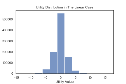
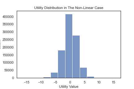
Figure A.1: Utility Distribution in Linear and Non-linear Settings

(a)	(b)

Notes: This figure depicts the distribution of users’ simulated utility in the linear case (Panel a) and the non-linear case (Panel b).

Appendix E Supplemental Experimental Details

We provide additional details in the live experiment, including attention check questions (Section 5.3), detailed item attributes in the four product categories (Section E.1), demographic survey and comparison of demographics between the training and testing sets (Section E.3), and full results (Section E.5).

E.1 Item Attributes

The following attributes are collected for each item for each category.

• Produce (22 attributes)

  • Dummy variables: organic; four allergens (milk, soy, egg, and fish)

  • Numerical variables: 2 size metrics (servingSizeGrams and servings); 13 ingredients (calories, caloricDensity, totalFat, saturatedFat, polyFat, monoFat, cholesterol, sodium, potassium, carbs, fiber, sugar, and protein); price; and health starpoints ranging from 0 to 4 with a higher value indicating a healthier option (see details in Howe et al. 2022).

• Meat, Dairy, and Eggs (40 attributes)

  • Dummy variables: organic; 14 subcategories; 9 allergens (nuts, coconut, almond, soy, sulfites, milk, wheat, fish, and shellfish)

  • Numerical variables: 2 size metrics (servingSizeGrams and servings); 14 ingredients (calories, caloricDensity, transFat, totalFat, saturatedFat, polyFat, monoFat, cholesterol, sodium, potassium, carbs, fiber, sugar, and protein); price; health starpoints

• Bakery, Pasta, and Grains (31 attributes)

  • Dummy variables: organic; 12 allergens (milk, egg, nuts, wheat, soy, sesame, almond, coconut, gluten, peanuts, pecans, and sulfites)

  • Numerical variables: 2 size metrics (servingSizeGrams and servings); 14 ingredients (calories, caloricDensity, transFat, totalFat, saturatedFat, polyFat, monoFat, cholesterol, sodium, potassium, carbs, fiber, sugar, and protein); price; health starpoints

• Beverage (38 attributes)

  • Dummy variables: organic; 8 subcategories; 12 allergens (milk, egg, nuts, wheat, soy, seasame, sulphur dioxide, coconut, gluten, sulfites, phenylalanine, and caffeine)

  • Numerical variables: 2 size metrics (servingSizeGrams and servings); 13 ingredients (calories, caloricDensity, totalFat, saturatedFat, polyFat, monoFat, cholesterol, sodium, potassium, carbs, fiber, sugar, and protein); price; health starpoints

E.2 Attention Check Questions

After reading the grocery task introduction, a participant is asked to answer the following questions

• In the task, you will imagine to be? Four options include evaluating pictures, watching videos, grocery shopping (the correct answer), and talking to a friend.

• In the grocery store task, you will imagine shopping with a budget of? Four options include $30, $50, $75 (the correct answer), and $100.

If a participant cannot correctly answer two questions above, he or she will be asked to read the instruction and answer the comprehension questions again. Upon answering the two questions correctly, the participant will proceed to the rest of the study.

E.3 Demographic Survey Questions

The demographic survey questions are as follows.

Single answer questions

• How would you describe your gender? Three options include male, female, and third gender (non-binary)

• What is the highest level of school you have completed or the highest degree you have received? 8 options include less than high school degree, high school graduate (high school diploma or equivalent including GED), some college but no degree, associate degree in college (2-year), bachelor’s degree in college (4-year), master’s degree, doctoral degree, and professional degree (JD, MD).

• Please indicate the answer that includes your entire household income in (previous year) before taxes. 13 options include less than $10,000; $10,000 to $19,999; $20,000 to $29,999; $30,000 to $39,999; $40,000 to $49,999; $50,000 to $59,999; $60,000 to $69,999; $70,000 to $79,999; $80,000 to $89,999; $90,000 to $99,999; $100,000 to $149,999; $150,000 or more; Prefer not to say.

• In which state do you currently reside? 52 options including fifty states, D.C. and Puerto Rico

• What religious family do you belong to or identify yourself most close to? 6 options include Buddhism, Jewish, Muslim, Christian (Catholic protestant or any other Christian denominations) , non-religious, and others (need specification).

• What is your height in feet and inches? Please choose your best estimate from 8 options include shorter than 5’1”, 5’1” to 5’2”, 5’3” to 5’4”, 5’5” to 5’6”, 5’7” to 5’8”, 5’9” to 5’10”, 5’11” to 6’0”, and taller than 6’0”.

• Indicate the extent (seven levels) to which you agree or disagree with each statement: i) I am on a diet; ii) I prefer organic food; iii) I like sweets; iv) I limit my calorie intake; v) I avoid eating too many carbs; vi) I avoid eating too much fat; vii) I avoid eating too much cholesterol; viii) I avoid eating too much salt.

Multiple answer questions

• Choose one or more races that you consider yourself to be. 6 options include White, Black or African American, American Indian or Alaska Native, Asian, Native Hawaiian or Pacific Islander , and others (need specification).

• Do you (or any immediate family member) have any dietary restrictions? 9 options include gluten-free, sugar-free, vegan, vegetarian, kosher, allergic to nuts, lactose intolerant, no restrictions, and others (need specification).

Open-ended questions

• What is your age?

• How many people live or stay in this household at least half the time?

• What is your current weight in pounds?

E.4 Demographic Comparison Between the Training and Testing Data

The experimental analyses presumes that the population-level hyper-parameters in the training and testing samples are the same. While the assumption is impossible to test, it is possible to assess the equality of means on the reported demographics.

Based on participants’ survey responses, we construct 119 demographic variables. For each variable, we conduct a t-test to compare the values for the training set and the testing set. Figure A.2 shows the distributions of the original p-values and Bonferroni-adjusted p-values (Cakanlar et al., 2022) across 119 tests. The Bonferroni-adjusted p-values indicate that participants in the training and testing sets are not statistically different.

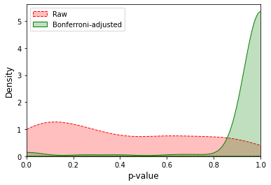
Figure A.2: Distribution of p-value of t-Test on Demographic Differences

Note: This figure portrays the distributions of the original p-values and Bonferroni-adjusted p-values for the t-test on the values of the demographic variables in the training set and in the testing set. The distributions are over the 119 tests corresponding to the 119 demographic variables.

E.5 Full Results

Table A.1 reports the cumulative HPR for each product category and aggregated across them.

Table A.1: Cumulative HPR (%) Results

Category	Method	$T=1$				$T=2$				$T=3$
		Num.Obs	cHPR	Improvement (%) by CFB-A		Num.Obs	cHPR	Improvement (%) by CFB-A		Num.Obs	cHPR	Improvement (%) by CFB-A
All	UCB	155	2.33	69.10 (12.21)***		127	2.34	68.38 (12.14)***		110	2.32	68.53 (11.31)***
	CFB	156	3.31	19.03 (4.37)***		126	3.34	17.96 (4.61)***		110	3.29	18.84 (4.51)***
	CFA	142	3.57	9.39 (2.58)***		121	3.62	8.84 (2.22)**		109	3.63	7.71 (1.83)**
	CFB-A	149	3.94	–		124	3.94	–		104	3.91	–
Produce	UCB	153	5.34	35.96 (4.85)***		126	4.93	47.67 (6.32)***		109	4.80	49.79 (6.59)***
	CFB	153	6.90	5.22 (0.80)		123	6.75	7.85 (1.24)		104	6.53	10.11 (1.56)*
	CFA	139	6.52	11.35 (1.93)**		123	6.54	11.31 (1.94)**		107	6.31	13.95 (2.38)***
	CFB-A	147	7.26	–		126	7.28	–		102	7.19	–
Meat, Dairy, and Eggs	UCB	134	2.31	59.40 (13.26)***		117	2.48	120.16 (12.25)***		103	2.52	112.70 (11.50)***
	CFB	131	4.16	36.78 (5.31)***		113	4.31	26.68 (4.21)***		101	4.32	26.62 (4.03)***
	CFA	123	5.29	7.56 (1.24)		109	5.34	2.25 (0.45)		101	5.36	2.05 (0.34)
	CFB-A	134	5.69	–		113	5.46	–		97	5.47	–
Bakery, Pasta, Grains	UCB	120	1.95	57.95 (6.34)***		107	2.09	44.50 (5.17)***		98	1.90	60.00 (6.53)***
	CFB	121	2.83	8.83 (1.21)		97	2.97	1.68 (0.29)		92	2.92	4.11 (0.60)
	CFA	117	2.91	5.84 (0.89)		99	2.98	1.34 (0.20)		94	3.13	-2.88 (-0.49)
	CFB-A	126	3.08	–		111	3.02	–		90	3.04	–
Beverages	UCB	81	1.04	37.5 (2.42)***		73	0.97	55.67 (3.52)***		73	0.92	68.48 (3.93)***
	CFB	74	1.68	-14.88 (-1.33)*		65	1.68	-10.12 (-1.11)		64	1.47	5.44 (0.56)
	CFA	87	1.48	-3.38 (-0.30)		71	1.65	-8.48 (-1.01)		69	1.72	-9.88 (-1.07)
	CFB-A	92	1.43	–		83	1.51	–		66	1.55	–

Notes: For a baseline model $m\in\left\{UCB,CFB,CFA\right\}$, the improvement (%) by CFB-A over $m$ is defined as $\frac{cHPR_{CFB-A}-cHPR_{m}}{cHPR_{m}}$; the best-performing model of each case is highlighted in bold. Significance levels of independent two-sample t-tests are denoted as follows: $*p<.10,**p<0.05,***p<.01$, and t-values are shown in parentheses.

References

- Abernethy et al. (2009) Abernethy, Jacob, Francis Bach, Theodoros Evgeniou, Jean-Philippe Vert. 2009. A new approach to collaborative filtering: Operator estimation with spectral regularization. Journal of Machine Learning Research 10(3).
- Agarwal et al. (2009) Agarwal, Deepak, Bee Chung Chen, Pradheep Elango, Nitin Motgi, Seung Taek Park, Raghu Ramakrishnan, Scott Roy, Joe Zachariah. 2009. Online models for content optimization. Advances in Neural Information Processing Systems 21 - Proceedings of the 2008 Conference. 17–24.
- Ahn (2008) Ahn, Hyung Jun. 2008. A new similarity measure for collaborative filtering to alleviate the new user cold-starting problem. Information Sciences 178(1) 37–51.
- Ansari et al. (2018) Ansari, Asim, Yang Li, Jonathan Z Zhang. 2018. Probabilistic topic model for hybrid recommender systems: A stochastic variational bayesian approach. Marketing Science 37(6) 987–1008.
- Aramayo et al. (Forthcoming) Aramayo, Nicolás, Mario Schiappacasse, Marcel Goic. Forthcoming. A multi-armed bandit approach for house ads recommendations. Marketing Science 0(0) null.
- Auer (2002) Auer, Peter. 2002. Using confidence bounds for exploitation-exploration trade-offs. Journal of Machine Learning Research 3(Nov) 397–422.
- Bayati et al. (2022) Bayati, Mohsen, Junyu Cao, Wanning Chen. 2022. Speed up the cold-start learning in two-sided bandits with many arms. arXiv preprint arXiv:2210.00340.
- Berman and Katona (2020) Berman, Ron, Zsolt Katona. 2020. Curation algorithms and filter bubbles in social networks. Marketing Science 39(2) 296–316.
- Bernstein et al. (2019) Bernstein, Fernando, Sajad Modaresi, Denis Sauré. 2019. A dynamic clustering approach to data-driven assortment personalization. Management Science 65(5) 2095–2115.
- Bertsimas and Mersereau (2007) Bertsimas, Dimitris, Adam J. Mersereau. 2007. A learning approach for interactive marketing to a customer segment. Operations Research 55(6) 1120–1135.
- Bobadilla et al. (2012) Bobadilla, Jesús, Fernando Ortega, Antonio Hernando, Jesús Bernal. 2012. A collaborative filtering approach to mitigate the new user cold start problem. Knowledge-Based Systems 26 225–238.
- Cakanlar et al. (2022) Cakanlar, Aylin, Remi Trudel, Katherine White. 2022. Political ideology and the perceived impact of coronavirus prevention behaviors for the self and others. Journal of the Association for Consumer Research 7(1) 36–44.
- Chen et al. (2019) Chen, Xinshi, Shuang Li, Hui Li, Shaohua Jiang, Yuan Qi, Le Song. 2019. Generative adversarial user model for reinforcement learning based recommendation system. International Conference on Machine Learning. PMLR, 1052–1061.
- Christakopoulou and Banerjee (2018) Christakopoulou, Konstantina, Arindam Banerjee. 2018. Learning to interact with users: A collaborative-bandit approach. SIAM International Conference on Data Mining, SDM 2018 (Section 3) 612–620.
- Christakopoulou et al. (2016) Christakopoulou, Konstantina, Filip Radlinski, Katja Hofmann. 2016. Towards conversational recommender systems. Proceedings of the 22nd ACM SIGKDD International Conference on Knowledge Discovery and Data Mining.
- Chu et al. (2011) Chu, Wei, Lihong Li, Lev Reyzin, Robert Schapire. 2011. Contextual bandits with linear payoff functions. Proceedings of the 14th International Conference on Artificial Intelligence and Statistics. JMLR Workshop and Conference Proceedings, 208–214.
- Cortes (2018) Cortes, David. 2018. Cold-start recommendations in collective matrix factorization. arXiv preprint arXiv:1809.00366.
- Cowgill and Tucker (2019) Cowgill, Bo, Catherine E Tucker. 2019. Economics, fairness and algorithmic bias. preparation for: Journal of Economic Perspectives.
- Dong et al. (2020) Dong, Bingbing, Yi Zhu, Lei Li, Xindong Wu. 2020. Hybrid collaborative recommendation via dual-autoencoder. IEEE Access 8 46030–46040.
- Farias and Li (2019) Farias, Vivek F, Andrew A Li. 2019. Learning preferences with side information. Management Science 65(7) 3131–3149.
- Filippi et al. (2010) Filippi, Sarah, Olivier Cappe, Aurélien Garivier, Csaba Szepesvári. 2010. Parametric bandits: The generalized linear case. Advances in Neural Information Processing Systems 23.
- Gangan et al. (2021) Gangan, Elena, Milos Kudus, Eugene Ilyushin. 2021. Survey of multi-armed bandit algorithms applied to recommendation systems. International Journal of Open Information Technologies 9(4) 12–27.
- Gardete and Santos (2020) Gardete, Pedro M, Carlos D Santos. 2020. No data? No problem! A search-based recommendation system with cold starts. arXiv preprint arXiv:2010.03455.
- Geng et al. (2022) Geng, Yishuai, Xiao Xiao, Xiaobing Sun, Yi Zhu. 2022. Representation learning: Recommendation with knowledge graph via triple-autoencoder. Frontiers in Genetics 13.
- Gomez-Uribe and Hunt (2015) Gomez-Uribe, Carlos A., Neil Hunt. 2015. The netflix recommender system: Algorithms, business value, and innovation. ACM Transactions on Management Information Systems 6(4) 1–19.
- Gonzalez Camacho and Alves-Souza (2018) Gonzalez Camacho, Lesly Alejandra, Solange Nice Alves-Souza. 2018. Social network data to alleviate cold-start in recommender system: A systematic review. Information Processing & Management 54(4) 529–544.
- Gordon et al. (2021) Gordon, Brett R., Kinshuk Jerath, Zsolt Katona, Sridhar Narayanan, Jiwoong Shin, Kenneth C. Wilbur. 2021. Inefficiencies in digital advertising markets. Journal of Marketing 85(1) 7–25.
- Guo et al. (2020) Guo, Dalin, Sofia Ira Ktena, Pranay Kumar Myana, Ferenc Huszar, Wenzhe Shi, Alykhan Tejani, Michael Kneier, Sourav Das. 2020. Deep bayesian bandits: Exploring in online personalized recommendations. Proceedings of the 14th ACM Conference on Recommender Systems. 456–461.
- Harpale and Yang (2008) Harpale, Abhay S, Yiming Yang. 2008. Personalized active learning for collaborative filtering. Proceedings of the 31st annual international ACM SIGIR conference on Research and development in information retrieval. 91–98.
- Harper and Konstan (2015) Harper, F. Maxwell, Joseph A. Konstan. 2015. The MovieLens datasets: History and context. ACM Transactions on Interactive Intelligent Systems 5 19:1–19:19.
- He et al. (2020) He, Xiangnan, Kuan Deng, Xiang Wang, Yan Li, Yongdong Zhang, Meng Wang. 2020. Lightgcn: Simplifying and powering graph convolution network for recommendation. Proceedings of the 43rd International ACM SIGIR conference on research and development in Information Retrieval. 639–648.
- Hosanagar et al. (2014) Hosanagar, Kartik, Daniel Fleder, Dokyun Lee, Andreas Buja. 2014. Will the global village fracture into tribes? Recommender systems and their effects on consumer fragmentation. Management Science 60(4) 805–823.
- Howe et al. (2022) Howe, Holly Samantha, Gavan J Fitzsimons, Peter Ubel. 2022. Open science online grocery: A tool for studying choice context and food choice. Journal of the Association of Consumer Research.
- Hu et al. (2019) Hu, Peng, Rong Du, Yao Hu, Nan Li. 2019. Hybrid item-item recommendation via semi-parametric embedding. IJCAI. 2521–2527.
- Hu et al. (2022) Hu, Saiquan, Juanjuan Zhang, Yuting Zhu. 2022. Zero to one: Sales prospecting with augmented recommendation. Available at SSRN 4006841.
- Jain and Pal (2022) Jain, Prateek, Soumyabrata Pal. 2022. Online low rank matrix completion. arXiv preprint arXiv:2209.03997.
- Jannach et al. (2020) Jannach, Dietmar, Gabriel de Souza P. Moreira, Even Oldridge. 2020. Why are deep learning models not consistently winning recommender systems competitions yet? A position paper. Proceedings of the Recommender Systems Challenge 2020. 44–49.
- Järvelin and Kekäläinen (2002) Järvelin, Kalervo, Jaana Kekäläinen. 2002. Cumulated gain-based evaluation of IR techniques. ACM Transactions on Information Systems (TOIS) 20(4) 422–446.
- Johari et al. (2021) Johari, Ramesh, Vijay Kamble, Yash Kanoria. 2021. Matching while learning. Operations Research 69(2) 655–681.
- Katehakis and Veinott (1987) Katehakis, Michael N, Arthur F Veinott. 1987. The multi-armed bandit problem: Decomposition and computation. Mathematics of Operations Research 12(2) 262–268.
- Kawale et al. (2015) Kawale, Jaya, Hung H Bui, Branislav Kveton, Long Tran-Thanh, Sanjay Chawla. 2015. Efficient Thompson sampling for online? Matrix factorization recommendation. Advances in Neural Information Processing Systems 28.
- Keskin et al. (2022) Keskin, N Bora, Yuexing Li, Nur Sunar. 2022. Data-driven clustering and feature-based retail electricity pricing with smart meters. Available at SSRN 3686518.
- Kille et al. (2015) Kille, Benjamin, Andreas Lommatzsch, Torben Brodt. 2015. News recommendation in real-time. Smart Information Systems. Springer, 149–180.
- Kokkodis and Ipeirotis (Forthcoming) Kokkodis, Marios, Panagiotis G Ipeirotis. Forthcoming. The good, the bad, and the unhirable: Recommending job applicants in online labor markets. Management Science 0(0) null.
- Koren et al. (2009) Koren, Yehuda, Robert Bell, Chris Volinsky. 2009. Matrix factorization techniques for recommender systems. Computer 42(8) 30–37.
- Korkut and Li (2021) Korkut, Melda, Andrew Li. 2021. Disposable linear bandits for online recommendations. Proceedings of the AAAI Conference on Artificial Intelligence, vol. 35. 4172–4180.
- Kotkov et al. (2016) Kotkov, Denis, Shuaiqiang Wang, Jari Veijalainen. 2016. A survey of serendipity in recommender systems. Knowledge-Based Systems 111 180–192.
- Kumar et al. (2020a) Kumar, Madhav, Dean Eckles, Sinan Aral. 2020a. Scalable bundling via dense product embeddings. arXiv preprint arXiv:2002.00100.
- Kumar et al. (2020b) Kumar, Rahul, Pradip Kumar Bala, Shubhadeep Mukherjee. 2020b. A new neighborhood formation approach for solving cold-start user problem in collaborative filtering. International Journal of Applied Management Science 12(2) 118–141.
- Kveton et al. (2017) Kveton, Branislav, Csaba Szepesvári, Anup Rao, Zheng Wen, Yasin Abbasi-Yadkori, S Muthukrishnan. 2017. Stochastic low-rank bandits. arXiv preprint arXiv:1712.04644.
- Lee and Hosanagar (2019) Lee, Dokyun, Kartik Hosanagar. 2019. How do recommender systems affect sales diversity? A cross-category investigation via randomized field experiment. Information Systems Research 30(1) 239–259.
- Li (2013) Li, Lihong. 2013. Generalized thompson sampling for contextual bandits. arXiv preprint arXiv:1310.7163.
- Li et al. (2012) Li, Lihong, Wei Chu, John Langford, Taesup Moon, Xuanhui Wang. 2012. An unbiased offline evaluation of contextual bandit algorithms with generalized linear models. JMLR: Workshop and Conference Proceedings 26 19–36.
- Li et al. (2010) Li, Lihong, Wei Chu, John Langford, Robert E. Schapire. 2010. A contextual-bandit approach to personalized news article recommendation. Proceedings of the 19th International Conference on World Wide Web, WWW ’10 661–670.
- Li et al. (2011) Li, Lihong, Wei Chu, John Langford, Xuanhui Wang. 2011. Unbiased offline evaluation of contextual-bandit-based news article recommendation algorithms. Proceedings of the 4th ACM International Conference on Web Search and Data Mining, WSDM 2011. 297–306.
- Li et al. (2016) Li, Shuai, Alexandros Karatzoglou, Claudio Gentile. 2016. Collaborative filtering bandits. Proceedings of the 39th International ACM SIGIR conference on Research and Development in Information Retrieval. 539–548.
- Liberali and Ferecatu (2022) Liberali, Gui, Alina Ferecatu. 2022. Morphing for consumer dynamics: Bandits meet hidden markov models. Marketing Science 41(4) 769–794.
- Lu et al. (2021) Lu, Yangyi, Amirhossein Meisami, Ambuj Tewari. 2021. Low-rank generalized linear bandit problems. International Conference on Artificial Intelligence and Statistics. PMLR, 460–468.
- McInerney et al. (2018) McInerney, James, Benjamin Lacker, Samantha Hansen, Karl Higley, Hugues Bouchard, Alois Gruson, Rishabh Mehrotra. 2018. Explore, exploit, and explain: Personalizing explainable recommendations with bandits. RecSys 2018 - 12th ACM Conference on Recommender Systems 31–39.
- Misra et al. (2019) Misra, Kanishka, Eric M. Schwartz, Jacob Abernethy. 2019. Dynamic online pricing with incomplete information using multi-armed bandit experiments. Marketing Science 38(2) 226–252.
- Nabi et al. (2022) Nabi, Sareh, Houssam Nassif, Joseph Hong, Hamed Mamani, Guido Imbens. 2022. Bayesian meta-prior learning using empirical bayes. Management Science 68(3) 1737–1755.
- Padilla and Ascarza (2021) Padilla, Nicolas, Eva Ascarza. 2021. Overcoming the cold start problem of customer relationship management using a probabilistic machine learning approach. Journal of Marketing Research 58(5) 981–1006.
- Resnick et al. (1994) Resnick, Paul, Neophytos Iacovou, Mitesh Suchak, Peter Bergstrom, John Riedl. 1994. GroupLens: An open architecture for collaborative filtering of netnews. Proceedings of the 1994 ACM Conference on Computer Supported Cooperative Work, CSCW 1994. 175–186.
- Rubens et al. (2015) Rubens, Neil, Mehdi Elahi, Masashi Sugiyama, Dain Kaplan. 2015. Active learning in recommender systems. Recommender systems handbook 809–846.
- Sardianos et al. (2017) Sardianos, Christos, Iraklis Varlamis, Magdalini Eirinaki. 2017. Scaling collaborative filtering to large–scale bipartite rating graphs using lenskit and spark. 2017 IEEE Third International Conference on Big Data Computing Service and Applications (BigDataService). IEEE, 70–79.
- Sarwar et al. (2001) Sarwar, Badrul, George Karypis, Joseph Konstan, John Riedl. 2001. Item-based collaborative filtering recommendation algorithms. Proceedings of the 10th International Conference on World Wide Web, WWW 2001. 285–295.
- Schwartz et al. (2017) Schwartz, Eric M., Eric T. Bradlow, Peter S. Fader. 2017. Customer acquisition via display advertising using multi-armed bandit experiments. Marketing Science 36(4) 500–522.
- Shi et al. (2014) Shi, Yue, Martha Larson, Alan Hanjalic. 2014. Collaborative filtering beyond the user-item matrix: A survey of the state of the art and future challenges. ACM Computing Surveys (CSUR) 47(1) 1–45.
- Silva et al. (2022) Silva, Nícollas, Heitor Werneck, Thiago Silva, Adriano CM Pereira, Leonardo Rocha. 2022. Multi-armed bandits in recommendation systems: A survey of the state-of-the-art and future directions. Expert Systems with Applications 197 116669.
- Song et al. (2019) Song, Yicheng, Nachiketa Sahoo, Elie Ofek. 2019. When and how to diversify? A multicategory utility model for personalized content recommendation. Management Science 65(8) 3737–3757.
- Strub et al. (2016) Strub, Florian, Romaric Gaudel, Jérémie Mary. 2016. Hybrid recommender system based on autoencoders. Proceedings of the 1st workshop on deep learning for recommender systems. 11–16.
- Su et al. (2016) Su, Jessica, Aneesh Sharma, Sharad Goel. 2016. The effect of recommendations on network structure. Proceedings of the 25th international conference on World Wide Web. 1157–1167.
- Tang et al. (2014) Tang, Liang, Yexi Jiang, Lei Li, Tao Li. 2014. Ensemble contextual bandits for personalized recommendation. Proceedings of the 8th ACM Conference on Recommender Systems. 73–80.
- Tang and Zhou (2012) Tang, Xiangyu, Jie Zhou. 2012. Dynamic personalized recommendation on sparse data. IEEE transactions on knowledge and data engineering 25(12) 2895–2899.
- Thompson (1933) Thompson, William R. 1933. On the likelihood that one unknown probability exceeds another in view of the evidence of two samples. Biometrika 25(3) 285–294.
- Trinh et al. (2020) Trinh, Cindy, Emilie Kaufmann, Claire Vernade, Richard Combes. 2020. Solving bernoulli rank-one bandits with unimodal thompson sampling. Algorithmic Learning Theory. PMLR, 862–889.
- Waisman et al. (2019) Waisman, Caio, Harikesh S Nair, Carlos Carrion, Nan Xu. 2019. Online causal inference for advertising in real-time bidding auctions. arXiv preprint arXiv:1908.08600.
- Wang and Blei (2011) Wang, Chong, David M Blei. 2011. Collaborative topic modeling for recommending scientific articles. Proceedings of the ACM SIGKDD International Conference on Knowledge Discovery and Data Mining. 448–456.
- Wang et al. (2016) Wang, Huazheng, Qingyun Wu, Hongning Wang. 2016. Learning hidden features for contextual bandits. Proceedings of the 25th ACM international on conference on information and knowledge management. 1633–1642.
- Wang et al. (2017) Wang, Huazheng, Qingyun Wu, Hongning Wang. 2017. Factorization bandits for interactive recommendation. Proceedings of the AAAI Conference on Artificial Intelligence 31(1).
- Wang et al. (2018) Wang, Qing, Chunqiu Zeng, Wubai Zhou, Tao Li, S Sitharama Iyengar, Larisa Shwartz, Genady Ya Grabarnik. 2018. Online interactive collaborative filtering using multi-armed bandit with dependent arms. IEEE Transactions on Knowledge and Data Engineering 31(8) 1569–1580.
- Wang et al. (2022) Wang, Y., L. Tao, X. Zhang. 2022. Recommending for a three-sided food delivery marketplace: A multi-objective hierarchical approach. Working paper.
- Wei et al. (2017) Wei, Jian, Jianhua He, Kai Chen, Yi Zhou, Zuoyin Tang. 2017. Collaborative filtering and deep learning based recommendation system for cold start items. Expert Systems with Applications 69 29–39.
- Wu (2018) Wu, Qingyun. 2018. Interactive online learning with incomplete knowledge. Working paper.
- Xing et al. (2014) Xing, Zhe, Xinxi Wang, Ye Wang. 2014. Enhancing collaborative filtering music recommendation by balancing exploration and exploitation. Proceedings of the 15th International Society for Music Information Retrieval Conference, ISMIR 2014 (Ismir) 445–450.
- Ye et al. (2020) Ye, Zikun, Dennis Zhang, Heng Zhang, Renyu Philip Zhang, Xin Chen, Zhiwei Xu. 2020. Cold start to improve market thickness on online advertising platforms: Data-driven algorithms and field experiments. Available at SSRN 3702786.
- Ying et al. (2006) Ying, Yuanping, Fred Feinberg, Michel Wedel. 2006. Leveraging missing ratings to improve online recommendation systems. Journal of Marketing Research 43(3) 355–365.
- Zhang et al. (2022) Zhang, Jiding, Ken Moon, Senthil K Veeraraghavan. 2022. Does fake news create echo chambers? Available at SSRN 4144897.
- Zhang et al. (2020) Zhang, Yan, Ivor W Tsang, Lixin Duan. 2020. Collaborative generative hashing for marketing and fast cold-start recommendation. IEEE Intelligent Systems 35(5) 84–95.
- Zhao et al. (2013) Zhao, Xiaoxue, Weinan Zhang, Jun Wang. 2013. Interactive collaborative filtering. Proceedings of the 22nd ACM international conference on Information & Knowledge Management. 1411–1420.
- Zheng et al. (2018) Zheng, Lei, Chun-Ta Lu, Fei Jiang, Jiawei Zhang, Philip S Yu. 2018. Spectral collaborative filtering. Proceedings of the 12th ACM conference on recommender systems. 311–319.
- Zhou (2015) Zhou, Li. 2015. A survey on contextual multi-armed bandits. arXiv preprint arXiv:1508.03326.
- Zhou et al. (2023) Zhou, Tongxin, Yingfei Wang, Lu Yan, Yong Tan. 2023. Spoiled for choice? personalized recommendation for healthcare decisions: A multiarmed bandit approach. Information Systems Research .