Non-cosmological, Non-Doppler Relativistic Frequency Shift over Astronomical Distances

Abstract

We investigate in detail an apparently unnoticed consequence of special relativity. It consists in time dilation/contraction and frequency shift for emitted light affecting accelerated reference frames at astronomical distances from an inertial observer. The frequency shift is non-cosmological and non-Doppler in nature. We derive the main formulae and compare their predictions with the astronomical data available for Proxima Centauri. We found no correspondence with observations. Since the implications of the new time dilation/contraction and frequency shift are blatantly paradoxical, we do not expect to find one. By all indications, we are dealing with a genuine, and not a merely apparent, relativity paradox.

Keywords: special relativity $\cdot$ time dilation/contraction $\cdot$ frequency shift $\cdot$ relativistic kinematics and dynamics $\cdot$ relativity paradox $\cdot$ Doppler shift $\cdot$ Proxima Centauri

1 Introduction

In the present paper, we focus on a consequence of special relativity that seems to have gone unnoticed. It consists in time dilation/contraction and consequent frequency shift for emitted light affecting accelerated reference frames at astronomical distances from an inertial observer. For these effects to show up, high relative velocities ($v\lesssim c$) are not necessary. The frequency shift derived hereafter is purely relativistic. It has nothing to do with the standard Doppler shift, which depends upon relative speed, nor with the cosmological redshift. These effects derive from a straightforward application of the Lorentz transformation of the time coordinate

$$t^{\prime}=\frac{t-\frac{vx}{c^{2}}}{\sqrt{1-\frac{v^{2}}{c^{2}}}},$$ (1)

where $t^{\prime}$ is the time coordinate of a frame moving with constant velocity $v$ along the $x$-direction of a stationary inertial reference frame with time coordinate $t$ (and parallel coordinate axes). As usual, $c$ stands for the velocity of light.

The phenomenon described here has already been discussed in [1] and is strictly related to the well-known Andromeda paradox [1, 2, 3, 4, 5].

In the following two sections, we derive the time dilation/contraction and the frequency shift formulae. Incidentally, they correspond to those derived from general relativity in the case of a weak and spatially uniform gravitational field. We shall show that these formulae also hold when the distant light source is inertial and stationary, and the observer accelerates.

In Section 4, we use these formulae to calculate the expected frequency shift of the light emitted by Proxima Centauri and compare it to the standard Doppler shift coming from the radial velocity imparted to the star by orbiting planet Proxima Centauri b. The aim is to see whether there are measurable consequences already for a relatively close astronomical source.

In Section 5, we shall discuss the import of these new time dilation/contraction and frequency shift phenomena. We show that despite the straightforward derivation, the predicted effects on the astronomical scale are loudly missing. Owing to the intrinsic paradoxical implications of the derived time dilation/contraction and frequency shift formulae, we expect not to find any observable effect. The fascinating aspect is that such paradoxes appear to have a genuine, and not a merely apparent, nature.

2 Quick Derivation of Purely Relativistic Time Dilation/Contraction and Frequency Shift

Consider two reference frames, $S$ and $S^{\prime}$. Initially, they are both inertial and relatively at rest, with parallel coordinate axes. Frame $S$ is the observer frame, while frame $S^{\prime}$ is the frame of the light source. Frame $S^{\prime}$ is placed at an astronomical distance $d$ from $S$ along its $x$-axis, with $d\gtrsim 1$ ly. With these initial conditions, $S$ and $S^{\prime}$ belong to the same plane of simultaneity, and their $t$-coordinates are the same, $t_{1}=t^{\prime}_{1}$.

Now, suppose that frame $S^{\prime}$ starts to accelerate with constant acceleration $\pm a$ along the $x$-axis of frame $S$ and maintains that acceleration until time $t_{2}$, with final velocity $a(t_{2}-t_{1})\ll c$. At that point, the system $S^{\prime}$ is a Lorentz system moving at a constant speed and, according to Equation (1), the instant $t^{\prime}_{2}$ of $S^{\prime}$ simultaneous with instant $t_{2}$ of $S$ is now given by

$$t^{\prime}_{2}=\frac{t_{2}-\frac{(\pm a)(t_{2}-t_{1})d}{c^{2}}}{\sqrt{1-\frac{a^{2}(t_{2}-t_{1})^{2}}{c^{2}}}}\approx t_{2}-\frac{(\pm a)(t_{2}-t_{1})d}{c^{2}},\quad\textrm{for}\,\,\,\frac{a(t_{2}-t_{1})}{c}\ll 1.$$ (2)

In Equation (2), we neglect terms containing the 2nd power of $v/c$. At time $t_{2}$, the position of $S^{\prime}$ relative to frame $S$ is no more $d$ but $d\pm\frac{1}{2}a(t_{2}-t_{1})^{2}$, but we neglect that because $\frac{1}{2}a(t_{2}-t_{1})^{2}\ll d$.

Notice that, although the relative velocity $a(t_{2}-t_{1})$ is much less than $c$, the simultaneity term $\frac{a(t_{2}-t_{1})d}{c^{2}}$ in Equation (2) is not negligible because of the large distance $d$.

Equation (2) tells us that while for the inertial observer in $S$, an interval of time $\Delta t=t_{2}-t_{1}$ has passed, the corresponding interval of time $\Delta t^{\prime}=t^{\prime}_{2}-t^{\prime}_{1}$ elapsed in reference frame $S^{\prime}$ is

$$\Delta t^{\prime}=\Delta t\left[1-\frac{(\pm a)d}{c^{2}}\right].$$ (3)

It is worth noticing that the application of Lorentz transformations to accelerated frames is a straightforward practice [6]. For instance, it has been used to provide a solution to the Bell spaceship paradox [7]. Even Einstein used it in 1905 to derive time dilation for a clock moving in a polygonal or continuously curved line [8]. In fact, in Section 3, we provide a derivation of our time dilation/contraction formula that makes use of and generalizes Einstein’s derivation by extending it to systems subject to constant acceleration for a short period of time. In the same section, a Minkowski diagram that visualizes the origin of the effect is also given.

Now, suppose that during interval $\Delta t^{\prime}$, the light source at rest in $S^{\prime}$ emits a beam of light of frequency $\nu^{\prime}$. That means that $N$ wave crests are emitted with $N=\nu^{\prime}\Delta t^{\prime}$. The same number of crests must then be received by the observer in $S$ exactly after the traveling time $d/c$, no matter how big $d/c$ is. Moreover, the observer in $S$ will receive the $N$ wave crests within the shorter interval of time $\Delta t$ because, for $S$, the whole emission process in $S^{\prime}$ has taken place within $\Delta t$ (the traveling time $d/c$ cannot affect that duration since $d/c$ is only a delay in receiving the wave train). That means that the observer in $S$ receives a beam of light of frequency $\nu$ such that $\nu\Delta t=N=\nu^{\prime}\Delta t^{\prime}$, and thus

$$\nu=\nu^{\prime}\left[1-\frac{(\pm a)d}{c^{2}}\right].$$ (4)

It is worth mentioning that Equations (3) and (4) correspond to those derived from general relativity in the approximation of a weak and spatially uniform gravitational field $\pm a$. In fact, within general relativity, they are obtained by using special relativity and the principle of equivalence.

It is useful for the subsequent derivations to define the dimensionless quantity $z$ as follows

$$z\equiv\frac{\nu-\nu^{\prime}}{\nu^{\prime}}=-\frac{\pm ad}{c^{2}}.$$ (5)

It is interesting to note that Equations (3) and (4) also hold if the source $S^{\prime}$ is inertial and stationary, and the observer $S$ accelerates with acceleration $\pm a$.

As before, $S$ and $S^{\prime}$ are initially inertial and relatively at rest, and thus $t_{1}=t^{\prime}_{1}$. Then, frame $S$ accelerates with acceleration $\pm a$ in the $x$-direction until the instant $t_{2}$ and afterward moves at constant velocity $\pm a(t_{2}-t_{1})$. From this moment onward, it does not matter which frame has accelerated and which is actually moving ($S$ with velocity $\pm a(t_{2}-t_{1})$ or $S^{\prime}$ with velocity $\mp a(t_{2}-t_{1})$). The Lorentz transformations are ‘memory-less’: in them, there is no mathematical dependence on the past motion history of the reference frames. Then, the relations that give $t_{2}^{\prime}$, $\Delta t^{\prime}$, and $\nu$ for $S$ are the same as Equations (2)–(4). We shall see later that this result has interesting philosophical consequences.

In the present and the following section, we have also adopted the same assumption made by Einstein in [9], namely that acceleration $a$ has negligible physical effects on the rate of clocks in the accelerated frame. That is known as the ‘clock hypothesis’ [10].

3 Detailed Derivation of the Time Dilation/Contraction Formula

Here, we take Einstein’s derivation of the time dilation formula for a clock moving in arbitrary motion (clock moving in a polygonal or continuously curved line [8]) and apply it to the case of a system moving on a straight line but subject to a uniform acceleration $a$ for a short period of time. Hereafter, without loss of generality, we assume that all the involved velocities are such that $v\ll c$. We shall see that when acceleration $a$ goes to zero, one recovers the well-known Einstein’s time dilation formula. On the other hand, if the distance between the inertial observer and the accelerating system is suitably large, one recovers Equation (3) of Section 2.

Consistently with the previous section, primed quantities refer to the moving system $S^{\prime}$, while non-primed ones refer to the inertial (stationary) system $S$. Moreover, $S^{\prime}$ moves in the positive $x$-direction of $S$, and all three coordinate axes are parallel. Suppose that $S^{\prime}$ initially moves with constant velocity $v_{1}$, and at time $t=t^{\prime}=0$ the origins of $S$ and $S^{\prime}$ overlap. Thus, the relation between the instants of time $t_{1}^{\prime}$ of $S^{\prime}$ and $t_{1}$ of $S$ is given by Equation (1) as follows

$$t_{1}^{\prime}=\frac{t_{1}-\frac{v_{1}(v_{1}t_{1})}{c^{2}}}{\sqrt{1-\frac{v_{1}^{2}}{c^{2}}}},$$ (6)

since $x_{1}=v_{1}t_{1}$.

At instant $t_{1}$, the system $S^{\prime}$ starts to accelerate in the positive or negative $x$-direction with constant acceleration $a$, and at instant $t_{2}$ returns to uniform motion with the new constant velocity $v_{2}=v_{1}\pm a(t_{2}-t_{1})$.

Thus, the relation between the instants of time $t_{2}^{\prime}$ of $S^{\prime}$ and $t_{2}$ of $S$ is now given by

$$t_{2}^{\prime}=\frac{t_{2}-\frac{[v_{1}\pm a(t_{2}-t_{1})][v_{1}t_{1}+v_{1}(t_{2}-t_{1})\pm\frac{1}{2}a(t_{2}-t_{1})^{2}]}{c^{2}}}{\sqrt{1-\frac{[v_{1}\pm a(t_{2}-t_{1})]^{2}}{c^{2}}}},$$ (7)

where $x_{2}=v_{1}t_{1}+v_{1}(t_{2}-t_{1})\pm\frac{1}{2}a(t_{2}-t_{1})^{2}$.

The interval of time $\Delta t^{\prime}=t_{2}^{\prime}-t_{1}^{\prime}$ is thus equal to

$$\Delta t^{\prime}=\frac{t_{2}-\frac{[v_{1}\pm a(t_{2}-t_{1})][v_{1}t_{1}+v_{1}(t_{2}-t_{1})\pm\frac{1}{2}a(t_{2}-t_{1})^{2}]}{c^{2}}}{\sqrt{1-\frac{[v_{1}\pm a(t_{2}-t_{1})]^{2}}{c^{2}}}}-\frac{t_{1}-\frac{v_{1}(v_{1}t_{1})}{c^{2}}}{\sqrt{1-\frac{v_{1}^{2}}{c^{2}}}}.$$ (8)

Now, it is not difficult to see that if we set $a=0$ in Equation (8) and do not neglect terms containing the 2nd power of $v/c$, we recover Einstein’s time dilation formula

$$\Delta t^{\prime}=\Delta t\sqrt{1-\frac{v_{1}^{2}}{c^{2}}}.$$ (9)

On the other hand, if we set $v_{1}t_{1}=d$, with $d$ equal to an extremely large astronomical distance, and if we consequently adopt the natural approximations, $v_{1}(t_{2}-t_{1})\pm\frac{1}{2}a(t_{2}-t_{1})^{2}\ll v_{1}t_{1}$ and $\frac{[v_{1}\pm a(t_{2}-t_{1})]^{2}}{c^{2}}\approx\frac{v_{1}^{2}}{c^{2}}\approx 0$ (we are now neglecting again terms containing the 2nd power of $v/c$), from Equation (8) we arrive at the following relation

$$\Delta t^{\prime}=\Delta t\left[1-\frac{\pm ad}{c^{2}}\right],$$ (10)

which is equal to Equation (3).

In short, we have replicated Einstein’s derivation of the time dilation for a clock arbitrarily moving relative to a stationary clock [8]. Like Einstein, we started from the Lorentz transformation of the time coordinate. However, we have plugged in the equation an explicit and simpler type of motion for the moving clock: namely, the moving clock moves away from the stationary one on a straight line at constant velocity $v_{1}$ for a time $t_{1}$, and then, for a time $(t_{2}-t_{1})$, it accelerates with a low acceleration $a$. That is simpler than Einstein’s motion in a polygonal or continuously curved line [8]. Therefore, if special relativity holds for non-uniform motion in a “continuously curved line”, it does also hold for a body slightly accelerating in a straight line. By the way, what we have done so far is equivalent to mapping the considered set-up onto a continuous sequence of events that are analyzed relative to instantaneous co-moving inertial frames.

In the remaining, we shall visualize the case with positive $a$ on a Minkowski diagram. To make the graph easily readable, we shall assume, along with the previous approximation $v/c\ll 1$, that the initial velocity $v_{1}$ of system $S^{\prime}$ is equal to zero, like in the case described in Section 2. Thus, until time $t_{1}$ (=$t_{1}^{\prime})$, systems $S$ and $S^{\prime}$ are relatively at rest. Then, from $t_{1}$ to $t_{2}$, system $S^{\prime}$ accelerates from $0$ to final velocity $a(t_{2}-t_{1})$, as seen from stationary system $S$.

As shown in Figure 1, the dot-dashed line represents the world line of a body placed at an astronomical distance $d$ in the reference frame $S^{\prime}$. Its world line is initially vertical because, until time $t_{1}$ $(=t_{1}^{\prime})$, both systems are relatively at rest. Then, between time $t_{1}$ and $t_{2}$, system $S^{\prime}$ and the body in it accelerate from $0$ to final velocity $a(t_{2}-t_{1})$.

Within $\Delta t=t_{2}-t_{1}$, the body’s world line gets bent to an angle $\theta$ relative to the $ct$ axis such that $\tan\theta=\frac{v}{c}=\frac{a(t_{2}-t_{1})}{c}$, and then it stays parallel to the $ct^{\prime}$ axis of $S^{\prime}$. Since $\frac{v}{c}=\frac{a(t_{2}-t_{1})}{c}\ll 1$, neglecting 2nd order terms in $v/c$, the unit lengths $U$ of space-time axes of $S$ and $S^{\prime}$ can be taken as identical,

$$U^{\prime}=U\sqrt{\frac{1+\frac{v^{2}}{c^{2}}}{1-\frac{v^{2}}{c^{2}}}}\approx U.$$ (11)

With reference to Figure 1, $\overline{BA}=ct_{2}-ct_{1}=c\Delta t$ and $\overline{C^{\prime}A^{\prime}}=ct_{2}^{\prime}-ct_{1}^{\prime}=c\Delta t^{\prime}$.

Since $\frac{v}{c}\ll 1$ and $\theta\approx 0$, we have that $\overline{C^{\prime}A^{\prime}}\approx\overline{CA}$ and $\overline{C^{\prime}B^{\prime}}\approx\overline{CB}$. Then, $c\Delta t-c\Delta t^{\prime}=\overline{BA}-\overline{C^{\prime}A^{\prime}}\approx\overline{BA}-\overline{CA}=\overline{CB}=d\tan\theta=\frac{vd}{c}=\frac{a(t_{2}-t_{1})d}{c}=\frac{a\Delta td}{c}$. Thus,

$$c\Delta t-c\Delta t^{\prime}=\frac{a\Delta td}{c}\quad\to\quad\Delta t^{\prime}=\Delta t\left[1-\frac{ad}{c^{2}}\right].$$ (12)

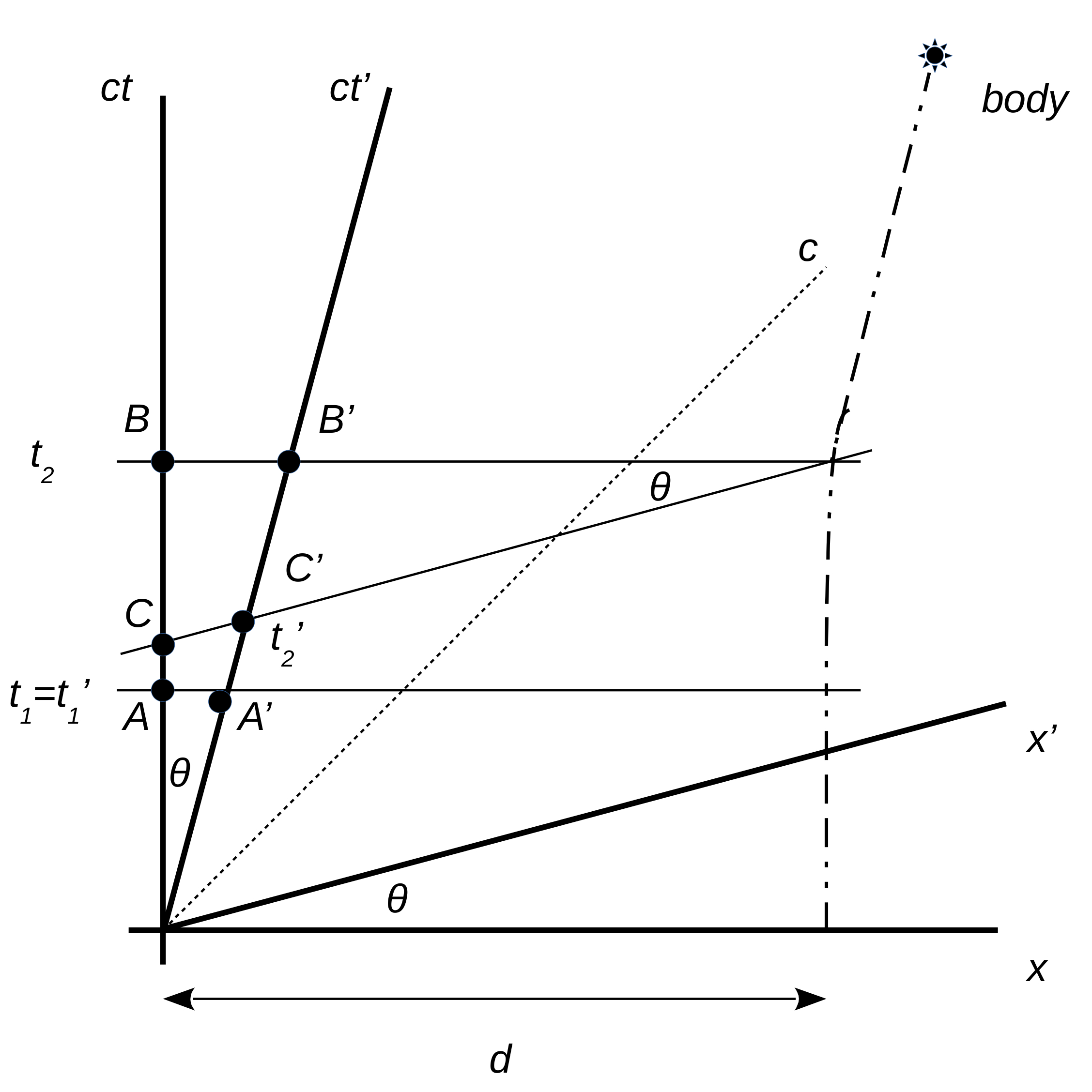
Figure 1: Minkowski diagram of a body at astronomical distance $d$ from a stationary observer (system $x$-$ct$). The body is at rest until time $t_{1}$ $(=t_{1}^{\prime})$ and then accelerates to the final constant speed $a(t_{2}-t_{1})$ in $\Delta t=t_{2}-t_{1}$. The dot-dashed line is the world line of the body. Quantities are not to scale. The magnitude of angle $\theta$ has been exaggerated for representation purposes.

4 Proxima Centauri

We now apply Equation (5) to the light emitted by Proxima Centauri at distance $d=4.25\,$ly ($d\simeq 4.02\times 10^{16}\,$m) to estimate the expected $z$ and compare it with the standard Doppler shift ascribable to the radial velocity of the star imparted by orbiting planet Proxima Centauri b.

In the scheme of Section 2, we assume Proxima Centauri to correspond to frame $S^{\prime}$, while we, the observers, are stationary in inertial frame $S$. Moreover, for the sake of derivation, we assume that we are on the orbital plane of Proxima b, and the acceleration of the star is along the line of sight.

Within that approximation and assuming a circular orbit, the projected position $r(t)$ of Proxima b relative to Proxima Centauri can be written as $r(t)=r_{0}\cos(\omega t)$, where $r_{0}=7.3\times 10^{9}\,$m is the planet semi-major axis and $\omega=\frac{2\pi}{T}$ with orbital period $T=11.18\,\textrm{d}=9.7\times 10^{5}\,$s. The mass of Proxima b is estimated to be $M_{Pr\,b}=9.6\times 10^{24}\,$kg, and the mass of Proxima Centauri is estimated to be $M_{Pr\,C}=2.4\times 10^{29}\,$kg. All the astronomical data are from [11].

The maximum value of Proxima b acceleration is given by $a_{Pr\,b}=|\ddot{r}(t)|_{max}$ $=r_{0}\omega^{2}\simeq 0.306\,$m/s². The maximum value of Proxima Centauri acceleration is then obtained by applying the third law of dynamics, $M_{Pr\,C}\cdot a_{Pr\,C}=m_{Pr\,b}\cdot a_{Pr\,b}$, giving $a_{Pr\,C}=\frac{m_{Pr\,b}}{M_{Pr\,C}}a_{Pr\,b}\simeq 1.21\times 10^{-5}\,$m/s².

Thus, the maximum absolute value of $z$ is

$$|z|_{max}=\left|\frac{\nu-\nu^{\prime}}{\nu^{\prime}}\right|=\frac{a_{Pr\,C}\cdot d}{c^{2}}\simeq 5.4\times 10^{-6}.$$ (13)

Let us compare this value with the maximum radial Doppler shift within the same approximation. The maximum value of Proxima b radial velocity is given by $v_{Pr\,b}=|\dot{r}(t)|_{max}$ $=r_{0}\omega\simeq 4.7\times 10^{4}\,$m/s. The maximum value of Proxima Centauri radial velocity is then obtained by applying the conservation of linear momentum, $M_{Pr\,C}\cdot v_{Pr\,C}=m_{Pr\,b}\cdot v_{Pr\,b}$, giving $v_{Pr\,C}=\frac{m_{Pr\,b}}{M_{Pr\,C}}a_{Pr\,b}\simeq 1.9\,$m/s.

Thus, the maximum absolute value of $z_{Doppler}=\pm\frac{v}{c}$ (for $v\ll c$) due to the standard Doppler shift is

$$|z|_{max\,Doppler}=\left|\frac{\nu-\nu^{\prime}}{\nu^{\prime}}\right|=\frac{v_{Pr\,C}}{c}\simeq 7.7\times 10^{-9}.$$ (14)

5 Discussion

In Sections 2 and 3, we have shown that the derivation of Equations (3) and (4) is straightforward and sound. However, as anticipated by the calculations in the preceding section, these new relations bring several issues with themselves that we shall discuss.

First and foremost, with the relatively close Proxima Centauri, the maximum frequency shift due to Equation (4) is expected to be three orders of magnitude larger than the maximum Doppler shift due to its radial velocity (Equations (13) and (14)). Unfortunately, no such phenomenon has been found in any observational data so far.

Moreover, as the distance $d$ between the emitting source and the Earth increases, the frequency shift should become more and more dramatic, let alone the fact that for suitably large $d$, we could have negative frequency $\nu$ and $\Delta t^{\prime}$. As far as this author knows, that has no immediate physical meaning.

A further problem comes from the case in which the light source always remains stationary in an inertial frame (frame $S^{\prime}$ inertial) while the observer accelerates (frame $S$ accelerating). As we have already shown at the end of Section 2, Equations (3)–(5) are still applicable to this case. Thus, suppose we are in that situation and now receive a light signal emitted with frequency $\nu^{\prime}$ by a source stationary in an inertial frame distant $d=$ 6 billion ly from us. Therefore, the signal was emitted 6 billion years ago. The point is: what would be the frequency $\nu$ of the light signal that we detect now? According to Equation (4), the frequency $\nu$ also depends upon our acceleration $a$ relative to the emitter at the epoch of the emission, then the actual value of $\nu$ is doomed to remain indeterminate. Six billion years ago, we did not exist as observers, not to mention the state of motion of our reference frame relative to the source back then. We have no doubt, though, that we do receive a definite frequency.

How can all this be settled? This last conundrum suggests that the problem may reside in the simultaneity term $-\frac{vx}{c^{2}}$ of the time coordinate transformation (1), particularly its dependence upon distance $x$.

In the end, our findings appear to be yet another relativity paradox. As usually happens with special relativity, every new paradoxical result, provided that it is formally correct, is always considered physically real. It is considered an inescapable consequence of special relativity, however counter-intuitive and lacking experimental confirmation may be.

With the present case, though, we believe there is something different going on. Here, we have macroscopic proofs (on the astronomical scale) that something is not working as expected in the machinery of special relativity, not from a mathematical but a physical point of view. We have no simple solution to this paradox. However, we believe that the problem is in itself real and worth to be described and discussing.

Funding

This research received no external funding.

Institutional Review Board Statement

Not applicable.

Informed Consent Statement

Not applicable.

Data Availability Statement

Not applicable.

Conflict of Interest

The author declares no conflict of interest.

References

- [1] D’Abramo, G. Astronomical distances and velocities and special relativity. arXiv, 2020, arXiv:1711.03833
- [2] C.W. Rietdijk, C.W. A rigorous proof of determinism derived from the special theory of relativity. Philos. Sci. 1966, 33, 341–344.
- [3] Putnam, H. Time and Physical Geometry. J. Philos. 1967, 64, 240–247.
- [4] Penrose, R. The Emperor’s New Mind: Concerning Computers, Minds, and the Laws of Physics; Oxford University Press: Oxford, UK, 1989; pp. 392–393.
- [5] Available online: https://en.wikipedia.org/wiki/Rietdijk-Putnam\_argument (accessed on 1 February 2022).
- [6] Desloge, E.A. and Philpott, R.J. Uniformly accelerated reference frames in special relativity. Am. J. Phys. 1987, 55, 252–261.
- [7] Franklin, J. Lorentz contraction, Bell’s spaceships, and rigid body motion in special relativity. Eur. J. Phys. 2010, 31, 291–298.
- [8] Einstein, A. On the Electrodynamics of Moving Bodies. Ann. Phys. 1905, 17, 891–921.
- [9] Einstein, A. On the relativity principle and the conclusions drawn from it. Jahrb. Radioakt. 1907, 4, 411–462.
- [10] Rosser, W. G. V. The clock hypothesis and the Lorentz transformations. Br. J. Philos. Sci. 1978, 29-4, 349–353.
- [11] Anglada-Escudé, G.; Amado, P.J.; Barnes, J.; Berdiñas, Z.M.; Butler, R.P.; Coleman, G.A.; de La Cueva, I.; Dreizler, S.; Endl, M.; Giesers, B.; et al. A terrestrial planet candidate in a temperate orbit around Proxima Centauri. Nature 2016, 536, 437–440.