D-Lite: Navigation-Oriented Compression of 3D Scene Graphs for Multi-Robot Collaboration

Abstract

For a multi-robot team that collaboratively explores an unknown environment, it is of vital importance that the collected information is efficiently shared among robots in order to support exploration and navigation tasks. Practical constraints of wireless channels, such as limited bandwidth, urge robots to carefully select information to be transmitted. In this letter, we consider the case where environmental information is modeled using a 3D Scene Graph, a hierarchical map representation that describes both geometric and semantic aspects of the environment. Then, we leverage graph-theoretic tools, namely graph spanners, to design greedy algorithms that efficiently compress 3D Scene Graphs with the aim of enabling communication between robots under bandwidth constraints. Our compression algorithms are navigation-oriented in that they are designed to approximately preserve shortest paths between locations of interest while meeting a user-specified communication budget constraint. The effectiveness of the proposed algorithms is demonstrated in robot navigation experiments in a realistic simulator. A video abstract is available at https://youtu.be/nKYXU5VC6A8.

10(3,.05)

This article has been accepted for publication at the IEEE Robotics and Automation Letters.

Please cite as: Yun Chang, Luca Ballotta, and Luca Carlone,

“D-Lite: Navigation-Oriented Compression of 3D Scene Graphs for Multi-Robot Collaboration”,

in IEEE Robotics and Automation Letters, 2023.

I Introduction

In the near future, robot teams will perform cooperative tasks in a multitude of application scenarios, ranging from exploration of subterranean environments, to search-and-rescue missions in hazardous settings, to human assistance in houses, airports, factory floors, and malls, to mention a few.

A key requirement for cooperative exploration and navigation in an initially unknown environment is to build a map model of the environment as the robots explore it. Recent work has proposed 3D Scene Graphs as an expressive hierarchical model of complex environments [1, 2, 3, 4, 5, 6]: a 3D Scene Graph organizes spatial and semantic information, including objects, structures (e.g., walls), places (i.e., free-space locations the robot can reach), rooms, and buildings into a graph with multiple layers corresponding to different levels of abstraction. 3D Scene Graphs provide a user-friendly model of the scene that can support the execution of high-level instructions by a human. Also, they capture traversability between places, rooms, and buildings that can be used for path planning.

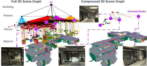
Figure 1: 3D Scene Graph of an environment (left) and compressed version produced by D-Lite (right). The purple circles mark the terminal nodes: D-Lite approximately preserves shortest-path distances between those locations of interest.

To scale up from single- to multi-robot systems and to longer missions and larger environments, a key challenge is to share the map information among the robots to support cooperation. For instance, the robots may exchange partial maps such that a robot can navigate within a portion of the environment mapped by another robot. However, the potentially high volume of data to be transferred over a shared wireless channel easily saturates the available bandwidth, degrading team performance. This holds true especially when the wireless channel is also used to transmit other information in the field —such as images or place recognition information for localization and map reconstruction— which further limits the bandwidth available for transmitting map information in a timely manner [7, 8, 9, 10]. The challenge of information sharing is particularly relevant when the map is modeled as a 3D Scene Graph, since these are rich and potentially large models if all nodes and edges are retained. On the other hand, 3D Scene Graphs also provide opportunities for compression: for instance, the robots may exchange information about rooms in the environment rather than sharing fine-grained traversability information encoded by the place layer; similarly, for a large-scale scene, the robot may just specify a sequence of buildings to be traversed, abstracting away geometric information at lower levels. This is similar to what humans do: when providing instructions to a person about how to reach a location in a building, we would specify a sequence of rooms and landmarks (e.g., objects or structures) rather than a detailed metric map or a precise path.

Therefore, the question we address in this paper is: how can we compress a 3D Scene Graph to retain relevant information the robots can use for navigation while meeting a communication budget constraint, expressed as the maximum size of the map the robots can transmit? Besides multi-robot communication, task-driven map compression can play a role in long-term autonomy under resource constraints, where the robots might suffer memory limitations and retain only key portions of a large map. Such a compression is also useful when it is desirable for the robots to share essential information under privacy considerations by sending only task-relevant data [11].

Related work. Graph compression is active area of research in discrete mathematics, computer science, and telecommunications, where it finds applications to, e.g., vehicle routing [12, 13], packet routing in wireless networks [14], and compression of unstructured data such as 3D point clouds [15, 16, 17].

A prominent body of works simplifies a graph by carefully pruning it based on structural properties of the graph. These methods typically entail some information loss, and aim to only retain relevant information when storing, processing, parsing, or transmitting the full graph is infeasible. For example, references [18, 14] find efficient representations of huge web and communication networks by heuristically selecting a few key elements, while the work [19] prunes graphs while preserving connectivity among nodes. Within the discrete mathematics literature, graph compression has been studied with focus on ensuring low distortion (or stretch) of inter-node distances. For example, spanning trees and Steiner trees are the smallest subgraphs maintaining connectivity in undirected graphs [20, 21]. Graph spanners remove a subset of edges while allowing for a user-defined maximum distortion of shortest paths [22, 23, 24]. A special case are distance preservers [25] that prune graphs but keep unaltered the distances for specified node pairs. Emulators are tools that replace a large number of edges with a few strategic ones to ensure small stretch of distances [26].

On the other hand, lossless compression strategies aim to find compact representations of graphs to be efficiently stored or processed. A subset of related work directly deals with communication-efficient re-labeling of nodes that enhance graph encoding. For example, some classical methods exploit algebraic tools such as spectral decomposition of the incidence or adjacency matrix that allow encoding the latter with a limited number of codewords, while paper [27] proposes an algorithm that exploits graph structures such as hubs and spokes. A recent survey of lossless compression techniques is given in [28]. A different paradigm for lossless compression is based on hypergraphs, which generalize standard graphs by allowing hyperedges that connect more than two nodes. Among others, paper [29] tailors semantic data compression, [30] proposes a procedure to construct hypergraphs from network data, [31, 32] tackle hypergraph partitioning, and [33] presents a signal processing framework based on hypergraphs.

Related work in robotics focuses on graph compression to speed up path planning and decision-making. Silver et al. [34] use Graph Neural Networks to detect key nodes by learning heuristic importance scores. Agia et al. [35] propose an algorithm that exploits the 3D Scene Graph hierarchy to prune nodes and edges not relevant to the robotic task. Targeting a related application domain, Tian et al. [36] study computation and communication efficiency of multi-robot loop closure, providing a strategy to share a limited number of visual features in multi-robot SLAM, while Denniston et al. [10] introduce a graph-based method to prune the multi-robot loop closures in order to save on processing time. Larsson et al. [37, 38, 39] propose algorithms to build hierarchical abstractions of tree-structured representations, for instance enabling fast planning on occupancy grid maps at progressively increasing resolution.

Novel contribution. In this paper, we tackle the challenging problem of efficiently sharing 3D Scene Graphs for navigation under hard communication constraints. We propose two greedy algorithms, BUD-Lite and TOD-Lite (collectively referred to as D-Lite), that leverage graph spanners to prune nodes and edges from a 3D Scene Graph while minimizing the distortion of the shortest paths between locations of interest (terminal nodes, see Fig. 1). Compared to the literature, our algorithms (i) are designed to retain navigation-relevant information, (ii) leverage the hierarchical structure of the 3D Scene Graph for compression, and (iii) enforce a user-specified size of the compressed 3D Scene Graph. Our algorithms are computationally efficient and apply to general 3D Scene Graphs. Furthermore, we allow for loose specifications of navigation tasks, to make our approach flexible to inexact or uncertain queries: for instance, a querying robot requesting a map from another robot may specify a number of potential location it has to navigate between, and this information is used by the queried robot for more effective 3D Scene Graph compression. To meet a sharp budget on transmitted information, we design suitable heuristics that exploit a graph spanner of the 3D Scene Graph to be sent: graph spanners allow to trade-off the size of a sub-graph of the 3D Scene Graph to be transmitted for the maximum distortion suffered by the shortest paths between nodes of interest. This helps us design compression algorithms with attention to time performance of navigation tasks, for which paths planned on the compressed graph are not much longer compared to paths computed from the original graph containing fine-scale spatial information.

In contrast, related works are either restricted to trees or involve mixed-integer programming [38, 37]. In particular, the approach in [37] builds geometric abstractions on-the-fly without considering semantic or hierarchical information of the graph to be compressed. Other pruning strategies do not directly target path planning tasks and focus on computational efficiency of local task-planning algorithms [35]. Finally, most works tailored to real-time compression do not allow for hard communication constraints, either turning to soft constraints in the form of Lagrangian-like regularization [37], or focusing on computational aspects with feasibility requirements [35]. In particular, the work [35] proposes to prune the 3D Scene Graph to boost efficiency of a local task-planning routine, but it does not allow for sharp bounds on the size of the pruned graph, and further assumes that a specific task is known beforehand and only needs to be efficiently planned by the robot (e.g., finding a way to grab and move specified objects).

The effectiveness of our algorithms is validated through realistic simulated experiments. We show that the proposed method meets hard communication constraints without excessively impacting navigation performance. For example, navigation time on the compressed graph increases by at most 8% after compressing the 3D Scene Graph to 1.6% of its size.

Paper organization. In Section II, we present the motivating setup for navigation-oriented compression in the presence of communication constraints, and states 3D Scene Graph compression as an optimization problem which can be exactly solved via Integer Linear Programming (ILP). To circumvent computational intractability of the ILP in practice, we design efficient algorithms that ensure to meet available communication resources while retaining spatial information useful for navigation. In particular, we leverage graph spanners to trad-off size of the compressed graph for distortion of shortest paths: mathematical background on spanners in provided in Section III, while explanation of our proposed algorithms is detailed in Section IV. In Section V, we test our approach with realistic simulation software for robotic exploration, and compare it to the compression approach in [37]. Final remarks and future research directions are given in Section VI.

II Navigation-Oriented Scene Graph Compression

Motivating scenario. We consider a multi-robot team exploring an unknown environment. Each robot navigates to gather information and builds a 3D Scene Graph (DSG) $\mathcal{G}=\left(\mathcal{V}_{\mathcal{G}},\mathcal{E}_{\mathcal{G}}\right)$ that describes the portion of the environment explored so far [1, 2, 3, 4]. As robots are scattered across a possibly large area, they exchange partial maps to collaboratively gather information about the environment. In particular, a robot $r_{1}$ may query another robot $r_{2}$ to get information about the area explored by $r_{2}$.

Navigation-oriented query. We assume that the querying robot $r_{1}$ needs to reach one or more target locations $\mathcal{T}\subset\mathcal{V}_{\mathcal{G}}$ within the DSG $\mathcal{G}=\left(\mathcal{V}_{\mathcal{G}},\mathcal{E}_{\mathcal{G}}\right)$ built by robot $r_{2}$. Such locations, for instance, may be objects or points of interest (e.g., the building exits). Hence, $r_{2}$ shall transmit its local map (i.e., nodes and edges of its DSG) such that $r_{1}$ can reach locations in $\mathcal{T}$ from a set $\mathcal{S}\subset\mathcal{V}_{\mathcal{G}}\setminus\mathcal{T}$ of source locations. In practice, the latter may represent physical access points (e.g., doors) at the boundary of the area explored by $r_{2}$ that are near $r_{1}$, and may be estimated by $r_{2}$ based on the current location of $r_{1}$. In the following, we generically refer to sources and targets as terminals (or terminal nodes), which for the sake of this work are assumed to be place nodes in the DSG.

Communication constraints. Data sharing among robots occurs over a common wireless channel. Because of resource constraints of wireless communication, such as limited bandwidth, robot $r_{2}$ cannot transmit its entire DSG to robot $r_{1}$. Specifically, we assume that robots can send only a small portion of their DSG each time they receive a share request. Hence, queried robot $r_{2}$ needs to compress its DSG $\mathcal{G}$ into a subgraph $\mathcal{G}^{\prime}=\left(\mathcal{V}_{\mathcal{G}^{\prime}},\mathcal{E}_{\mathcal{G}^{\prime}}\right)$, with $\mathcal{V}_{\mathcal{G}^{\prime}}\subseteq\mathcal{V}$ and $\mathcal{E}_{\mathcal{G}^{\prime}}\subseteq\mathcal{E}$, that contains at most $B$ nodes (where the budget $B$ reflects the available bandwidth) in order to comply with communication constraints, while at the same time retaining information useful for robot $r_{1}$ to navigate between the terminal nodes.

Pruning 3D Scene Graphs. Assuming navigation-oriented queries, the relevant information reduces to nodes and edges describing efficient paths robot $r_{1}$ can use to move across the map. Specifically, the collection of all shortest paths between a source $s\in\mathcal{S}$ and target $t\in\mathcal{T}$ is the least information ensuring that navigation by $r_{1}$ takes the shortest possible time, i.e., the time a robot with full knowledge of the map would take.

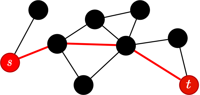
(a) Full graph (length $3$).

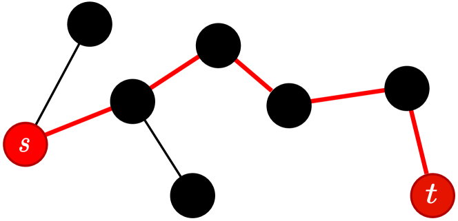
(b) Pruned graph (length $5$).

Figure 2: Distortion of shortest path from $s$ to $t$ (thick red).

However, transmitting all nodes in the shortest paths may violate the communication constraint (see Fig. 6): this can happen with many terminals or if shortest paths have little overlap. Hence, heavier pruning of the DSG might be needed to make communication feasible. This means that information useful for path planning will be partially unavailable to the querying robot’s planner. In other words, because the DSG $\mathcal{G}$ cannot be fully sent, the distance (length of a shortest path) between a pair of terminals in the transmitted graph $\mathcal{G}^{\prime}$ will be larger than the distance between those same terminals in the original DSG. A schematic example is provided in Fig. 2, where the length of the shortest path between nodes $s$ and $t$ increases from $3$ to $5$ after node and edge removal. For example, a robot may prune place nodes within a room, or share only the room node as a coarse representation of places. This requires less communication, but the querying robot $r_{1}$, which receives a coarser map, will be forced to, e.g., take a longer detour across a room, instead of traversing the original shortest path along a set of place nodes. Mathematically, this means $d_{\mathcal{G}^{\prime}}(s,t)\geq d_{\mathcal{G}}(s,t)$ for any $s\in\mathcal{S}$ and for any $t\in\mathcal{T}$, where $d_{\mathcal{G}}(u,v)$ is the distance from node $u$ to node $v$ in $\mathcal{G}$.

Problem formulation. For the querying robot $r_{1}$ to navigate efficiently, the distance $d_{\mathcal{G}^{\prime}}(s,t)$ between $s\in\mathcal{S}$ and $t\in\mathcal{T}$ in the transmitted graph $\mathcal{G}^{\prime}$ should not be much larger than the distance in the original graph $\mathcal{G}$. Hence, the queried robot $r_{2}$ shall prune $\mathcal{G}$ so as to minimize the distortion, or stretch, between shortest paths in the original and compressed graphs, while meeting the communication budget $B$. This can be cast into the following optimization problem: G’⊆Gβ d_G’(s,t)≤d_G(s,t) + βW_max^G(s,t)  ∀(s,t)∈P |V_G’|≤B, where $W_{\text{max}}^{\mathcal{G}}(u,v)$ is the maximum edge weight on a shortest path from $u$ to $v$ in $\mathcal{G}$ and $\mathcal{P}\subseteq\mathcal{S}\times\mathcal{T}$ is the set of considered source-target pairs. Constraint (2) ensures that the amount of transmitted information (number of nodes) meets the communication constraint, while constraint (II) and cost (2) encode minimization of the maximum distortion incurred by the shortest paths. The coefficient $W_{\text{max}}^{\mathcal{G}}(s,t)$ in (II) makes the distortion computation meaningful for weighted graphs.

Problem (2) can be solved by means of integer linear programming (ILP), see Appendix A. However, the runtime complexity of ILP solvers is subject to combinatorial explosion, making this approach impractical for online operation. Hence, we propose greedy algorithms that require lighter-weight computation, based on graph spanners.

III background: graph spanners

We ground our compression algorithm in the concept of graph spanner [22]. In words, a spanner is a compressed (i.e., sparse) representation of a graph such that shortest paths between nodes are distorted at most by a user-defined stretch. Formally, a spanner $\mathcal{G}^{\prime}=\left(\mathcal{V},\mathcal{E}^{\prime}\right)$ of graph $\mathcal{G}=\left(\mathcal{V},\mathcal{E}\right)$ is a subgraph such that $\mathcal{E}^{\prime}\subseteq\mathcal{E}$ and the following inequality holds for $u,v\in\mathcal{V}$,

$$d_{\mathcal{G}^{\prime}}(u,v)\leq\alpha d_{\mathcal{G}}(u,v)+\beta W_{\text{max}}^{\mathcal{G}}(u,v),$$ (1)

where $\alpha\geq 1$ and $\beta\geq 0$ are given constants. For generic $\alpha$ and $\beta$, $\mathcal{G}^{\prime}$ is called an $(\alpha,\beta)$-spanner, whereas if $\beta$ (resp. $\alpha$) is equal to zero (resp. one) $\mathcal{G}^{\prime}$ is called $\alpha$-multiplicative spanner (resp. $\beta$-additive or $+\beta$ spanner). Inequality (1) may hold for all nodes in $\mathcal{G}$ or for a few pairs as in (II): in the latter case, the resulting subgraph is referred to as a pairwise spanner.

Applications of spanners include navigation or packet routing in large graphs, whose size makes running path planning algorithms in the original graph computationally infeasible, [13, 40]. In this case, one can compute a spanner of the original graph and run planning algorithms on the spanner instead.

As one can see from (1), the characterization of spanners shares similarity with problem (2). Unfortunately, no method is known in the literature to build a spanner given a fixed node (or edge) budget, whereas algorithms usually enforce stretch (1) given input parameters $\alpha$ and $\beta$ while attempting to minimize the total spanner edge-weight to obtain lightweight representations. The standard formulation of the graph spanner problem can be then written as follows [22, Problem 2], E_G’⊆E_∑_(i,j)∈E_G’W^G(i,j) d_G’(s,t)≤αd_G(s,t) + βW_max^G(s,t), where $W^{\mathcal{G}}(i,j)$ is the weight of edge $(i,j)$ and the objective function for unweighted graphs reduces to counting the number of edges. For multiplicative spanners this problem was quickly solved, with the classical work [41] proposing and analyzing a greedy algorithm which is known to be the best (in terms of spanner size) that runs in polynomial time. Additive and $(\alpha,\beta)$-spanners are instead more complex to build, and many algorithms have been proposed in the literature: early efforts were devoted to unweighted graphs [42, 43, 44, 45], while subsequent work has focused on the general weighted case [24, 46, 47, 48]. Other studies are concerned with distributed [49] and dynamical [50] methods, Euclidean graphs [51], and reachability preservation in digraphs [52], to mention a few.

To the best of our knowledge, the only paper to address the presence of an edge budget $E_{\text{max}}$ is [23]. However, the algorithm proposed in [23] receives in input also parameters $\alpha$ and $\beta$, and checks feasibility of an $(\alpha,\beta)$-spanner with at most $E_{\text{max}}$ edges. Furthermore, its runtime increases exponentially with $E_{\text{max}}$, making it unsuitable for robotics applications.

A possible way to tackle the problem at hand is to iteratively build spanners with larger and larger distortion, until the budget is met. However, several issues can hamper such a strategy. First, running a spanner-building algorithm several times may be time-consuming. Second, while small-sized (i.e., with $O(n^{1+\varepsilon(\alpha)})$ edges, for some small $\varepsilon(\alpha)>0$) multiplicative spanners can be built for any given constant coefficient $\alpha\geq 1$, few constant-distortion additive spanner constructions are known for weighted graphs, with coefficient $\beta\in\{2,4,6\}$. Conversely, polynomial distortion $\beta=\beta(n)$ is needed to build additive spanners with near-linear size [44], thus the trade-off between spanner size and path distortion is not easy to exploit.

An important point is that multiplicative and additive distortions may yield dramatic differences in paths induced by the spanner. In particular, multiplying path length by a constant factor in large graphs may be undesirable in practice: for example, if a navigation task nominally takes one hour, stretching it to two or three hours yields substantial performance degradation. Conversely, additive stretch is usually preferred because it provides a constant time overhead, which is why we used this kind of distortion in our problem formulation.

In the following, we illustrate a heuristic procedure that allows us to meet the budget constraint in (2), runs in real time, and enforces a low distortion of shortest paths as measured by condition (II).

IV 3D scene graph compression algorithms

We propose D-Lite, a compression method for DSGs to meet communication constraints with attention to navigation efficiency. We design two versions of D-Lite, which are initialized with a spanner of the full DSG (Section IV-B) and tackle the compression problem from opposite perspectives.

The first algorithm, BUD-Lite (Section IV-C), performs progressive bottom-up compression of the spanner computed during initialization, exploiting the DSG abstraction hierarchy. In contrast, the second algorithm, TOD-Lite (Section IV-D), works top-down expanding nodes with the spanner as a target.

IV-A Intuition and the Role of the 3D Scene Graph Hierarchy​​​

Ideally, navigation-oriented compression of a DSG would require searching among all possible subgraphs of $\mathcal{G}$ to find one that minimally stretches paths between terminals. Such a search is prone to combinatorial blow-up and is thus impractical.

Assume we want to design a greedy procedure that removes nodes and edges in $\mathcal{G}$ while limiting the incurred path stretch. This goal is subject to a nontrivial trade-off. On the one hand, to ensure low stretch (i.e., retain navigation performance), it is desirable to parse one or a few nodes at each iteration so as to introduce extra distortion in a controlled way. On the other hand, parsing too few nodes at each time induces a large number of total iterations, and is computationally expensive for online operation. Hence, an effective algorithm should effectively choose the size of node batch to be greedily compressed at each iteration to strike a balance between compression quality and runtime.

To this aim, we crucially exploit the hierarchical structure of the DSG. We refer to a node $m$ that is adjacent to node $n$ in the upper layer as a child of $n$ to stress the hierarchical semantics of the DSG, and symmetrically call node $n$ the parent of $m$. The children of $n$ in graph $\mathcal{G}$ are denoted by $C_{\mathcal{G}}(n)$. Also, the set $\mathcal{E}_{\mathcal{G}}(n)$ gathers all edges incident to $n$ in $\mathcal{G}$. The DSG hierarchy allows us to see a node as a “compressed”, or “abstract”, representation of its children. Hence, transmitting $n$ rather than $C_{\mathcal{G}}(n)$ saves communication and conveys partial spatial information about nodes in $C_{\mathcal{G}}(n)$. For instance, let $C_{\mathcal{G}}(n)$ represent places inside a room and $n$ the associated room node. A robot that needs to reach a location $t\in C_{\mathcal{G}}(n)$ (e.g., the door) in that room with no bandwidth constraints can be provided with a sequence of places to reach $t$. Alternatively, the robot can be given the room node $n$ and it needs to explore the room to find the target $t$: this extra exploration , (corresponding to additional path stretch in the compressed DSG) takes longer, degrading navigation performance, but allows for compression to meet communication constraints. The navigation time for local exploration (e.g., to reach a place from the room centroid) is encoded by the weights of edges connecting non-finest resolution nodes or nodes at different resolutions (layers). For our experiments, we derive such weights from the full DSG as detailed in Appendix B. However, we argue that a robot can estimate all weights on-the-fly (while building the DSG) based on the actual navigation time it experiences.

The discussion above suggests a simple way to compress the DSG: a greedy procedure can be devised so that nodes in a layer can be progressively replaced by their parent nodes in the layer above. Every time we replace nodes with more “abstract” ones (rooms, buildings) the length of the paths passing through those nodes increases, indicating longer navigation. Hence, we can opportunistically select which nodes to “abstract away” so as to achieve a small stretch in the paths between terminals. In alternative, we can start with a coarse representation (including only the highest abstraction level) and expand it to reduce the stretch of the paths. We present these two greedy strategies below and initialize both procedures by computing a spanner of the given DSG, as explained next.

IV-B Building a DSG Spanner

Both proposed algorithms build a spanner of the DSG during initialization. A detailed description of how each procedure uses this spanner is deferred to Sections IV-C and IV-D.

Algorithm 1 describes how to build a spanner of the DSG that enforces a user-defined maximum additive stretch for distances between specified terminal pairs in $\mathcal{P}$. We adapt our algorithm from [24, Section 5]. Specifically, the procedure [24] can trade spanner size for stretch according to input parameters, building a $+cn^{\frac{1-\varepsilon}{2}}\alpha W_{\text{max}}^{\mathcal{G}}$ spanner of size $O(n^{1+\varepsilon})$. That algorithm is intended for generic spanners (not pairwise), hence we adapt it to our scope by retaining only nodes and edges needed to connect terminal pairs in $\mathcal{P}$, and deleting all others. Algorithm 1 is composed of two sequential stages: an initialization phase that builds a temporary spanner $\mathcal{G}^{\prime\prime}$ with a small number of edges that attempts to keep low initial path distortions, and a "buying" phase where edges are added to meet the stretch constraint. The initialization selects edges in three ways: performing a $d$-light initialization [47, Section 2] with appropriate $d$ (Algorithm 1), which in words ensures that each node has some initial neighbors; randomly picking cross-layer edges to exploit the DSG hierarchy (Algorithm 1); adding a greedy multiplicative spanner [41, Section 2] to reduce large path distortions (Algorithm 1). Then, for each pair $(s,t)$ the shortest path $P_{\mathcal{G}^{\prime\prime}}(s,t)$ from source $s$ to target $t$ in the temporary spanner $\mathcal{G}^{\prime\prime}$ is considered (in suitable order): in case the stretch in $\mathcal{G}^{\prime\prime}$ exceeds the constraint, edges and nodes from a shortest path in the original graph $\mathcal{G}$ are added to both $\mathcal{G}^{\prime\prime}$ and the final spanner $\mathcal{G}^{\prime}$ (Lines 1–1), otherwise, the shortest path in $\mathcal{G}^{\prime\prime}$ is directly added to the final spanner $\mathcal{G}^{\prime}$ (Algorithm 1). We refer to this subroutine as build_spanner.

Input: DSG $\mathcal{G}$, terminal pairs $\mathcal{P}$, user parameters $\varepsilon>0,p\in[0,1],\alpha>2,c>0$.

Output: DSG spanner $\mathcal{G}^{\prime}$.

1 $\mathcal{G}^{\prime}_{1}\leftarrow n^{\varepsilon}$-light initialization of $\mathcal{G}$;

2 $\mathcal{G}^{\prime}_{2}\leftarrow$ random sample of cross-layer edges of $\mathcal{G}$ w.p. $p$;

3 $\mathcal{G}^{\prime}_{3}\leftarrow$ $\alpha$-multiplicative spanner of $\mathcal{G}$;

$\mathcal{G}^{\prime\prime}\leftarrow\mathcal{G}^{\prime}_{1}\cup\mathcal{G}^{\prime}_{2}\cup\mathcal{G}^{\prime}_{3}$;

  // to compute paths

4 $\mathcal{G}^{\prime}\leftarrow\mathcal{P}$;

5 foreach $(s,t)\in\mathcal{P}$ do // sorted by $W_{\text{max}}^{\mathcal{G}}(s,t)$

6       if $d_{\mathcal{G}^{\prime\prime}}(s,t)>d_{\mathcal{G}}(s,t)+cn^{\frac{1-\varepsilon}{2}}\alpha W_{\text{max}}^{\mathcal{G}}(s,t)$ then

7             $\mathcal{G}^{\prime\prime}\leftarrow\mathcal{G}^{\prime\prime}\cup P_{\mathcal{G}}(s,t)$;

8             $\mathcal{G}^{\prime}\leftarrow\mathcal{G}^{\prime}\cup P_{\mathcal{G}}(s,t)$;

9            

10      else

11             $\mathcal{G}^{\prime}\leftarrow\mathcal{G}^{\prime}\cup P_{\mathcal{G}^{\prime\prime}}(s,t)$;

12            

13      

return $\mathcal{G}^{\prime}$.

Algorithm 1 Build spanner

Before diving into the core of our compression algorithms, it is worth reinforcing the motivation to use graph spanners. Algorithm 1 outputs a spanner with given maximal stretch of shortest paths, but does not guarantee that the produced spanner matches the desired node budget ${B}$. As noted in Section III, we cannot straightly apply a state-of-the-art spanner construction because no real-time algorithm in the literature addresses the presence of an exact budget. However, building a spanner greatly reduces the graph to be compressed up front, retaining only nodes and edges which both are relevant for navigation and sharply enhance efficiency of our proposed compression strategies. Moreover, even though path distortion may be increased to satisfy communication requirements, the user-defined stretch guaranteed by the spanner algorithm allows us to start from a maximum desired distortion: hence, if the latter is chosen loose enough, we may expect that the spanner output by Algorithm 1 is already somewhat close to the communication constraint, so that additional distortion will not be very high. In particular, the spanner construction leverages overlapping portions of paths to select a handful of key edges and nodes, whereas other navigation-efficient constructions, such as the collection of all shortest paths, do not exploit the graph structure to enhance compression. Furthermore, there are no tight bounds for the size of shortest paths, hence one cannot predict how much paths will be stretched in order to meet the communication budget.

IV-C BUD-Lite: a bottom-up compression algorithm

The idea behind our first algorithm (BUD-Lite, short for Bottom-Up D-Lite) is to iteratively compress the DSG spanner produced by Algorithm 1. The mechanism is simple: we progressively replace batches of nodes with their parents to reduce size, while attempting to keep the stretch incurred by the shortest paths between terminals low.

To gain intuition, consider Fig. 3 that illustrates three steps of BUD-Lite on a toy DSG. Dashed edges and light-colored nodes are part of the full DSG $\mathcal{G}$ and can be added to the compressed DSG $\mathcal{G}^{\prime}$. The latter is marked with solid lines and brighter colors. The first iteration of BUD-Lite parses the path from $s$ to $t_{1}$ and abstracts away place nodes $P_{3}$ and $P_{4}$, which are replaced with room node $R_{2}$ that is a coarse representation of those places (top right). Room $R_{1}$ is skipped because it does not reduce budget as compared to keeping $P_{1}$. Place $P_{2}$ is not removed yet because it lies also on the path connecting pair $(s,t_{2})$, while $P_{5}$ is still needed to connect $(s,t_{1})$. Node $P_{2}$ is removed at the second round when the path from $s$ to $t_{2}$ is parsed and shortcut through place node $P_{1}$ and room node $R_{2}$ (bottom right). The final step parses the last portion of the path connecting $(s,t_{1})$ and abstracts away the remaining places $P_{5}$ and $P_{6}$ under rooms $R_{2}$ and $R_{3}$ (bottom left). An example on an actual DSG build from simulated data is shown in Fig. 4, where the room node is used to abstract several places. More results on DSGs from simulated navigation data are provided in Appendix D.

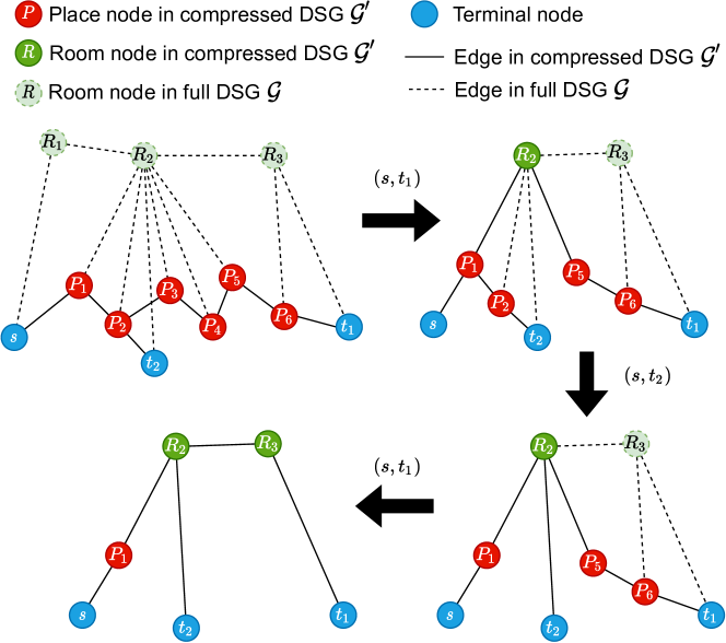
Figure 3: Illustration of the BUD-Lite procedure with source $s$ and targets $t_{1},t_{2}$. At each iteration, place nodes in a shortest path between terminals are replaced by a room node. Nodes are removed when none of the terminal pairs $(s,t_{1})$ and $(s,t_{2})$ connects through them. Note that the final graph cannot be further pruned without disconnecting terminals.

We formally introduce the compression procedure in Algorithm 2. The compressed graph is initialized as the DSG spanner $\mathcal{G}^{\prime}$ output by Algorithm 1 (Algorithm 2). In the following, the symbol $\mathcal{L}_{i}^{\mathcal{G}}$ refers to the nodes within the $i$th layer of $\mathcal{G}$. For example, $\mathcal{L}_{0}^{\mathcal{G}}$ collects all place nodes of the full DSG $\mathcal{G}$. Also, $P_{\mathcal{G}}(s,t)$ denotes the shortest path between $s$ and $t$ in $\mathcal{G}$. The external loop at Algorithm 2 parses each layer $\mathcal{L}_{i}^{\mathcal{G}^{\prime}}$ of $\mathcal{G}^{\prime}$, starting from the bottom ($i=0$) and moving to the upper layer $\mathcal{L}_{i+1}^{\mathcal{G}^{\prime}}$ after $\mathcal{L}_{i}^{\mathcal{G}^{\prime}}$ has been compressed (Algorithm 2). At each iteration of the inner loop at Algorithm 2, the algorithm checks if the shortest path connecting terminals $s$ and $t$ in $\mathcal{G}^{\prime}$ is traversed by nodes in layer $\mathcal{L}_{i}^{\mathcal{G}^{\prime}}$ with the same parent node $n\in\mathcal{L}_{i+1}^{\mathcal{G}}$ (Algorithm 2): if this is the case, such nodes with common parent are removed from $P_{\mathcal{G}^{\prime}}(s,t)$ and replaced (compressed) with their parent node $n$ (Algorithm 2). Such a compression in the graph causes a corresponding stretch of the actual path followed by the robot, the amount of which depends on both the involved layer $\mathcal{L}_{i}^{\mathcal{G}^{\prime}}$ and the number of compressed nodes, in light of the discussion in Section IV-A. The nested structure of Algorithm 2 looping over layers externally (Algorithm 2) and over paths internally (Algorithm 2) adds one abstraction level at a time for each path (the layer $\mathcal{L}_{i}^{\mathcal{G}^{\prime}}$ is fixed in loop Algorithm 2), and hence stretches distances in a balanced fashion: for example, if paths are made of places nodes, the first iteration of the inner loop compresses only one room for each path, so that at no point during the compression procedure a path is overly compressed with respect to other paths (i.e., it is not possible that a path is entirely abstracted to room nodes while another is kept with all places nodes). In general, this allows fine-scale spatial information to be retained as long as possible, and coarser layers (e.g., buildings) to be used only after finer layers (e.g., rooms) have been fully exploited for all paths (i.e., building nodes can be used only if all paths contain room nodes and no places nodes, possibly except for terminal nodes). To ensure paths are always feasible, we use a data structure $\mathcal{D}$ to track which paths are using nodes in $\mathcal{G}^{\prime}$ (Algorithm 2): only when a node is traversed by no path (Lines 2 to 2), it is removed. For BUD-Lite to terminate, the budget $B$ has to accommodate at least minimal-cardinality paths between terminals, which we assume holds true.

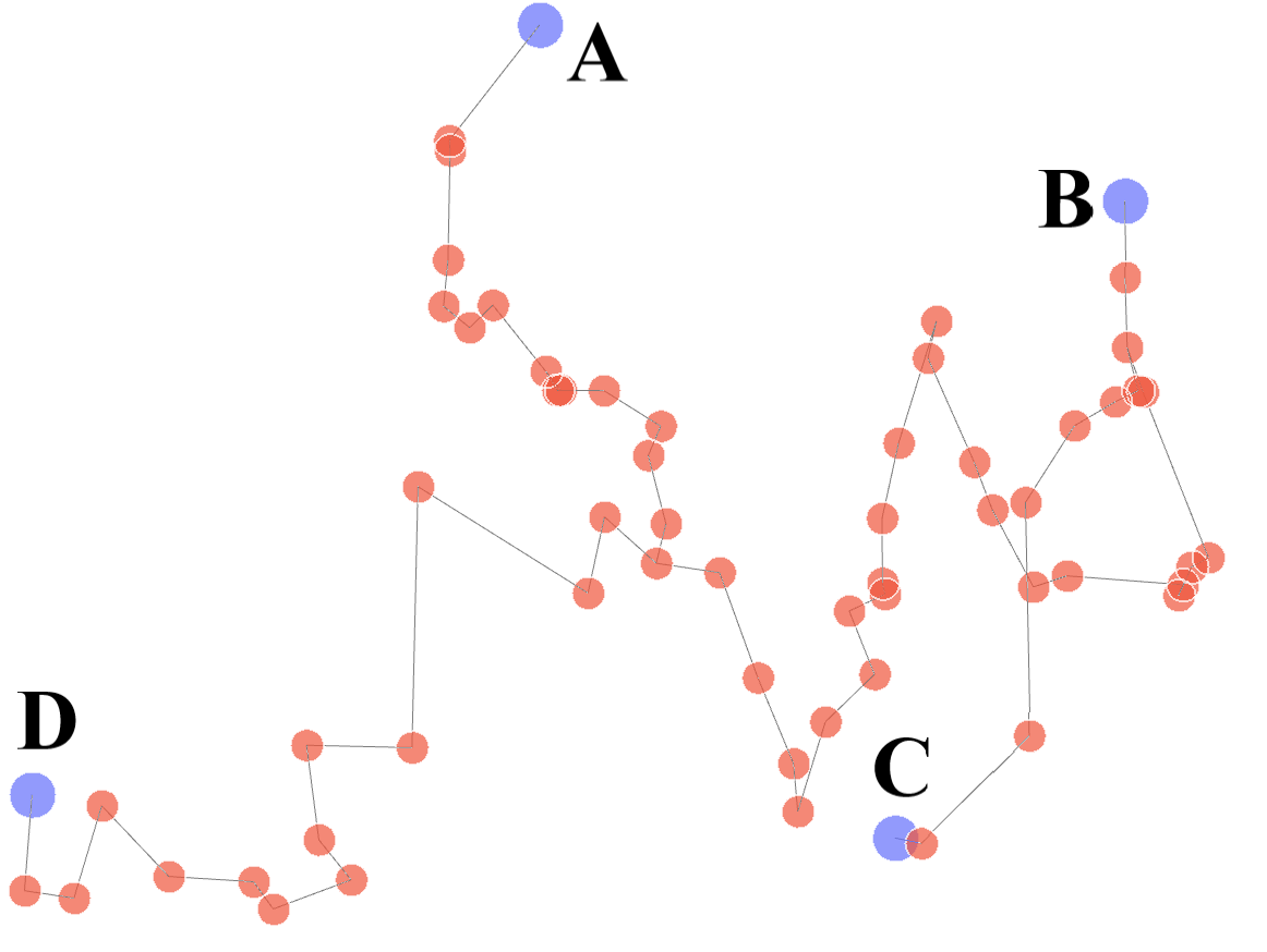
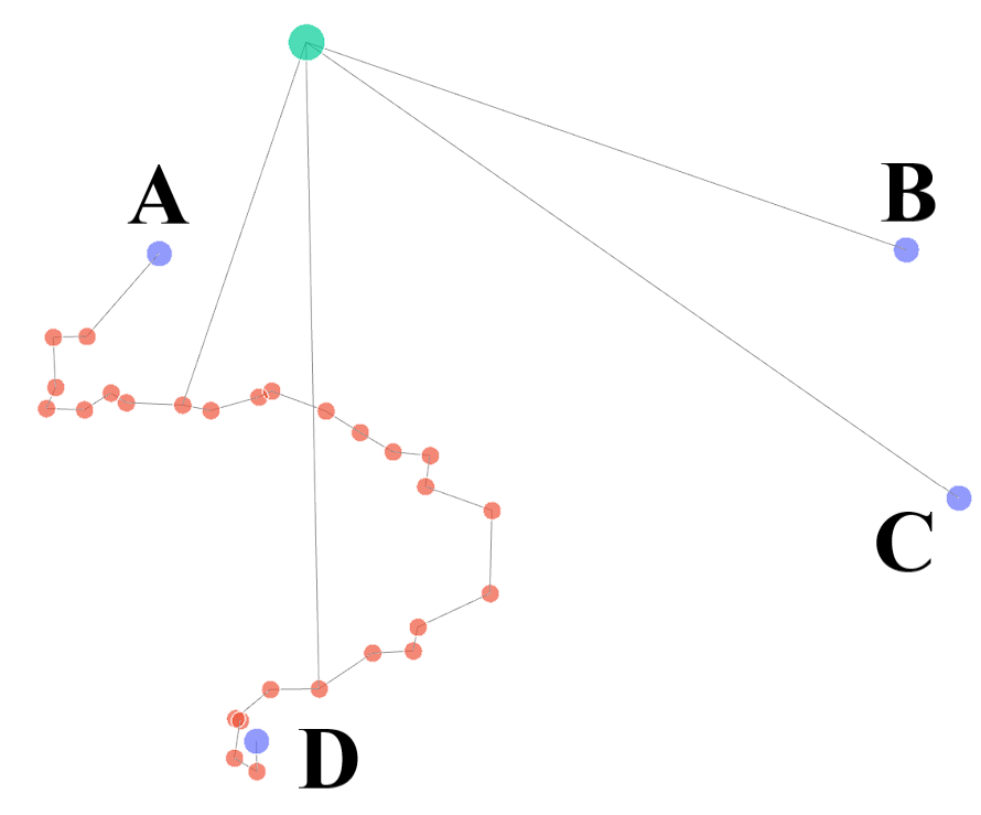
Figure 4: Initial (left) and final DSG (right). Terminal nodes (A, B, C, and D) are in blue, place nodes in red, and the room node in green.

Input: DSG $\mathcal{G}$, terminal pairs $\mathcal{P}$, node budget ${B}$.

Output: Compressed DSG $\mathcal{G}^{\prime}$.

$\mathcal{G}^{\prime}\leftarrow$ build_spanner$\left(\mathcal{G},\mathcal{P}\right)$;

  // initialization

1 foreach $n\in\mathcal{V}_{\mathcal{G}^{\prime}}$ do // track node usage

2       $\mathcal{D}{\left[n\right]}\leftarrow\{(s,t)\in\mathcal{P}:n\in P_{\mathcal{G}^{\prime}}(s,t)\}$;

3      

4for $i=0,\dots,L-1$ do // parse layers bottom-up

5       while $\mathcal{L}_{i}^{\mathcal{G}^{\prime}}\neq\emptyset$ do // parse layer till empty

6             foreach $(s,t)\in\mathcal{P}$ do // parse path from $s$ to $t$

7                   if $\exists n\in\mathcal{L}_{i+1}^{\mathcal{G}}:P_{\mathcal{G}^{\prime}}(s,t)\cap C_{\mathcal{G}^{\prime}}(n)\neq\emptyset$ then

8                         replace $P_{\mathcal{G}^{\prime}}(s,t)\cap C_{\mathcal{G}^{\prime}}(n)$ with $n$ in $P_{\mathcal{G}^{\prime}}(s,t)$;

9                         $\mathcal{D}{\left[n\right]}\leftarrow\mathcal{D}{\left[n\right]}\cup{(s,t)}$;

10                         foreach $m\in P_{\mathcal{G}^{\prime}}(s,t)\cap C_{\mathcal{G}^{\prime}}(n)$ do

11                               $\mathcal{D}{\left[m\right]}\leftarrow\mathcal{D}{\left[m\right]}\setminus{(s,t)}$;

12                               if $\mathcal{D}{\left[m\right]}=\emptyset$ then // prune DSG

13                                     $\mathcal{V}_{\mathcal{G}^{\prime}}\leftarrow\mathcal{V}_{\mathcal{G}^{\prime}}\setminus\left\{m\right\}$;

14                                     $\mathcal{E}_{\mathcal{G}^{\prime}}\leftarrow\mathcal{E}_{\mathcal{G}^{\prime}}\setminus\mathcal{E}_{\mathcal{G}^{\prime}}(m)$;

15                                    

16                              

17                        if $|\mathcal{V}_{\mathcal{G}^{\prime}}|\leq{B}$ then // budget is met

18                               return $\mathcal{G}^{\prime}$.

19                        

20                  

21            

22      

Algorithm 2 BUD-Lite

Performance bound. We now provide an analytical bound on the worst-case stretch that is incurred by every shortest path after running BUD-Lite. First, we provide two definitions that are instrumental to the understanding of the bound.

Definition 1 (Ancestor).

The ($i$th) ancestor $a_{\mathcal{G}}^{i}(n)$ of node $n\in\mathcal{L}_{i_{0}}^{\mathcal{G}}$ is the unique node in layer $\mathcal{L}_{i}^{\mathcal{G}}$, $i>i_{0}$, that is connected to $n$ by a path composed of only cross-layer edges.

In words, the ancestors of node $n$ are coarse representations of $n$ in upper layers. For example, the first two ancestors of a place node are its room and building nodes, respectively.

Definition 2 (Diameter).

For any node $n\in\mathcal{V}_{\mathcal{G}}$, its diameter $\mathrm{diam}_{\mathcal{G}}(n)$ is the maximum cardinality of all shortest paths connecting two children nodes of $n$ in $\mathcal{G}$, that is,

$$\mathrm{diam}_{\mathcal{G}}(n)\doteq\max\left\{|P_{\mathcal{G}}(c_{1},c_{2})|:c_{1},c_{2}\in C_{\mathcal{G}}(n)\right\},$$ (2)

where $|P_{\mathcal{G}}(c_{1},c_{2})|$ denotes the number of nodes in $P_{\mathcal{G}}(c_{1},c_{2})$.

In words, the diameter of a node describes how “large” the node is when expanded into its children in the layer below.

We now assume the following bounds on quantities associated with the original DSG $\mathcal{G}$. Recall that any edge $(m,n)\in\mathcal{E}_{\mathcal{G}}$ with $m,n\in\mathcal{V}_{\mathcal{G}}$ is assigned a weight $W^{\mathcal{G}}(m,n)$.

Assumption 1 (DSG bounds).

For any layer $i\in\left\{1,\dots,L\right\}$,

$$\begin{split}W_{\text{max}}^{i}&\doteq\max\left\{W^{\mathcal{G}}(m,n):m,n\in\mathcal{L}_{i}^{\mathcal{G}}\right\},\\ W_{\text{max}}^{i-1,i}&\doteq\max\left\{W^{\mathcal{G}}(m,n):m\in\mathcal{L}_{i-1}^{\mathcal{G}},n\in\mathcal{L}_{i}^{\mathcal{G}}\right\},\\ u_{\text{min}}^{i}&\doteq\min\left\{\left|P_{\mathcal{G}}(a_{\mathcal{G}}^{i}(s),a_{\mathcal{G}}^{i}(t))\right|:(s,t)\in\mathcal{P}\right\},\\ \mathrm{diam}_{\text{min}}^{i}&\doteq\min\left\{\mathrm{diam}_{\mathcal{G}}(n):n\in\mathcal{L}_{i}^{\mathcal{G}}\right\}.\end{split}$$ (3)

• $W_{\text{max}}^{i}$ is the maximum weight of edges in layer $\mathcal{L}_{i}^{\mathcal{G}}$;

• $W_{\text{max}}^{i-1,i}$ is the maximum weight of cross-layer edges between layers $\mathcal{L}_{i-1}^{\mathcal{G}}$ and $\mathcal{L}_{i}^{\mathcal{G}}$;

• $u_{\text{min}}^{i}$ is the minimum cardinality of a shortest path between the $i$th ancestors of every two connected terminals;

• $\mathrm{diam}_{\text{min}}^{i}$ is the minimum diameter of nodes in layer $\mathcal{L}_{i}^{\mathcal{G}}$.

Equipped with the definition above, we can bound the distortion on the compressed DSG $\mathcal{G}^{\prime}$ provided by BUD-Lite.

Proposition 1 (Worst-case BUD-Lite stretch).

After $k$ total iterations of the innermost loop in Algorithm 2, the distance between any two terminals in the compressed graph $\mathcal{G}^{\prime}$ is

$$d_{\mathcal{G}^{\prime}}(s,t)\;\leq\;2\sum_{i=1}^{\ell_{\text{max}}}W_{\text{max}}^{i-1,i}+\left(u_{\text{min}}^{\ell_{\text{max}}-1}-\alpha_{k}\mathrm{diam}_{\text{min}}^{\ell_{\text{max}}}\right)W_{\text{max}}^{\ell_{\text{max}}-1}\\ +\alpha_{k}W_{\text{max}}^{\ell_{\text{max}}},\quad\forall(s,t)\in\mathcal{P},$$ (4)

where

$$\alpha_{k} \doteq\left\lceil\dfrac{k}{|\mathcal{P}|}-\sum_{i=\ell_{0}}^{\ell_{\text{max}}-1}u_{\text{min}}^{i}\right\rceil,$$ (5)

$$\ell_{\text{max}} \doteq\max\left\{\ell:k>|\mathcal{P}|\sum_{i=\ell_{0}}^{\ell-1}u_{\text{min}}^{i}\right\},$$ (6)

$$\ell_{0} \doteq\!\begin{multlined}\max\left\{\ell:\min_{(s,t)\in\mathcal{P}}\left(d_{\mathcal{G}}(s,t)+\beta W_{\text{max}}^{\mathcal{G}}(s,t)\right)\geq\right.\\ \left.2\sum_{i=1}^{\ell}W_{\text{min}}^{i-1,i}+u_{\text{min}}^{\ell}W_{\text{min}}^{\ell}\right\}.\end{multlined}\max\left\{\ell:\min_{(s,t)\in\mathcal{P}}\left(d_{\mathcal{G}}(s,t)+\beta W_{\text{max}}^{\mathcal{G}}(s,t)\right)\geq\right.\\ \left.2\sum_{i=1}^{\ell}W_{\text{min}}^{i-1,i}+u_{\text{min}}^{\ell}W_{\text{min}}^{\ell}\right\}.$$ (9)

Proof.

See Appendix C. ∎

In words, $\ell_{0}$ is the index of the bottom layer in the initial spanner $\mathcal{G}^{\prime}$ in Algorithm 2 (excluding terminals); $\ell_{\text{max}}$ is the index of the top (coarsest) layer reached by BUD-Lite after $k$ total iterations; $\alpha_{k}$ is the number of nodes in the latter layer that have been added to the compressed graph after $k$ iterations. In the bound (4), the first term is the stretch due to cross-layer edges connecting the terminals to nodes in the upper layers, while the other terms are the stretch due to the shortest path passing partially across the coarsest layer $\mathcal{L}_{\ell_{\text{max}}}^{\mathcal{G}}$ (third term) and partially across layer $\mathcal{L}_{\ell_{\text{max}}-1}^{\mathcal{G}}$ (second term).

IV-D TOD-Lite: a Top-Down Expansion Algorithm

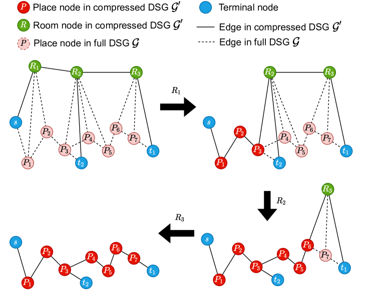
Figure 5: Illustration of the TOD-Lite expansion procedure with one source $s$ and two targets $t_{1}$ and $t_{2}$. At each iteration, a room node is expanded and replaced with its children place nodes. Adjacent nodes may be added to ensure connectivity (e.g., $P_{3}$ at first iteration).

This section presents our second greedy algorithm. Symmetrically to the bottom-up approach of Algorithm 2, the idea behind TOD-Lite (short for TOp-down D-Lite) is to exploit the DSG hierarchy by expanding node children to iteratively increase spatial granularity of the compressed graph (Fig. 5).

The idea of TOD-Lite is depicted with a toy example in Fig. 5, where room nodes $R_{1}$, $R_{2}$, and $R_{3}$ are progressively replaced with their respective children (place nodes). The initial condition (top left) contains the minimum set of nodes that guarantee connectivity between terminals, and it features coarse spatial abstractions through the retained nodes.

We formally describe TOD-Lite in Algorithm 3. During initialization, Algorithm 3 builds a spanner $\mathcal{G}^{\prime}_{\text{target}}$ of the DSG with Algorithm 1, which is used as target for the final compressed graph $\mathcal{G}^{\prime}$ (Algorithm 3). Then, it populates a “hierarchical spanner” $\mathcal{H}$ (Algorithm 3): this is simply a graph obtained from the original DSG $\mathcal{G}$ by keeping the spanner $\mathcal{G}^{\prime}_{\text{target}}$ plus nodes and edges encountered starting from $\mathcal{G}^{\prime}_{\text{target}}$ and going up the DSG hierarchy all the way to the top layer. Elements unrelated to the ancestors of $\mathcal{G}^{\prime}_{\text{target}}$ are removed. For example, if $\mathcal{G}^{\prime}_{\text{target}}$ is made of place nodes, $\mathcal{H}$ includes $\mathcal{G}^{\prime}_{\text{target}}$, the room nodes associated with those places (with cross-layer edges), and possibly nodes above in the hierarchy, e.g., the buildings containing those rooms. Graph $\mathcal{H}$ is used to expand nodes from coarser to finer layers, as explained next. To define an expansion priority for nodes in the same layer, a data structure $\mathcal{D}$ stores how many paths pass though each node in the graph, including both original paths in the target spanner (Algorithm 3) and path abstractions in upper layers (Algorithm 3): for example, the priority of a room node $R$ is given by the number of paths actually passing through $R$ in $\mathcal{G}^{\prime}_{\text{target}}$ and of paths traversing places nodes associated with $R$.

The main phase is an iterative top-down expansion through the hierarchical spanner $\mathcal{H}$. The output graph $\mathcal{G}^{\prime}$ is initialized with terminal nodes and paths that connect them under minimal communication budget: these are obtained by connecting each source-target pair to their common ancestor at minimal distance through cross-layer edges (Lines 3 to 3). Then, starting from the top layer $\mathcal{L}_{L}^{\mathcal{G}^{\prime}}$ and going down one layer at a time (Algorithm 3), each node in $\mathcal{G}^{\prime}$ is expanded (Algorithms 3, 3 and 3) till such operation is infeasible (Algorithm 3). In particular, if a node $n\in\mathcal{G}^{\prime}$ has a set of children $C_{\mathcal{H}}(n)$ in the hierarchical spanner $\mathcal{H}$, then Algorithm 3 removes $n$ from $\mathcal{G}^{\prime}$ and Algorithm 3 adds to $\mathcal{G}^{\prime}$ nodes in $C_{\mathcal{H}}(n)$ and their incident edges $\mathcal{E}_{\mathcal{H}}(C_{\mathcal{H}}(n))$.

Expanding nodes gradually restores the geometric granularity of the DSG spanner, because a spatially coarse representation (e.g., room node) is replaced by a group of nodes with fine resolution (e.g., place nodes). This expansion comes at the price of heavier communication burden. Nonetheless, using the hierarchical spanner allows us to narrow the expansion procedure to a small set of navigation-relevant nodes, both saving runtime and helping meet communication constraints.

Input: DSG $\mathcal{G}$, terminal pairs $\mathcal{P}$, node budget ${B}$.

Output: Compressed DSG $\mathcal{G}^{\prime}$.

1 $\mathcal{G}^{\prime}_{\text{target}}\leftarrow$ build_spanner$\left(\mathcal{G},\mathcal{P}\right)$;

2 $\mathcal{H}\leftarrow$ hierarchical spanner from $\mathcal{G}^{\prime}_{\text{target}}$;

3 foreach $n\in\mathcal{V}_{\mathcal{G}^{\prime}_{\text{target}}}$ do // for expansion priority

4       $\mathcal{D}{\left[n\right]}\leftarrow\big{|}\{(s,t)\in\mathcal{P}:n\in P_{\mathcal{G}^{\prime}_{\text{target}}}(s,t)\}\big{|}$;

5      

6for $i=1,\dots,L$ do

7       foreach $n\in\mathcal{L}_{i}^{\mathcal{H}}$ do

8             $\mathcal{D}{\left[n\right]}\leftarrow\sum_{n^{\prime}\in\mathcal{V}_{\mathcal{H}}\left(n\right)}\mathcal{D}{\left[n^{\prime}\right]}$;

9            

10      

$\mathcal{V}_{\mathcal{G}^{\prime}}\leftarrow\mathcal{P}$;

  // add terminals

11 foreach $(s,t)\in\mathcal{P}$ do // add cheapest path from $s$ to $t$

12       $a\leftarrow$ lowest common ancestor of $s$ and $t$ in $\mathcal{H}$;

13       $\mathcal{V}_{\mathcal{G}^{\prime}}\leftarrow\mathcal{V}_{\mathcal{G}^{\prime}}\cup\left\{a\right\}$;

14       $\mathcal{E}_{\mathcal{G}^{\prime}}\leftarrow$ edges connecting $s$ and $t$ with $a$ in $\mathcal{G}^{\prime}$;

15      

16for $i=L,\dots,1$ do // parse layers top-down

17       foreach $n\in\mathcal{L}_{i}^{\mathcal{G}^{\prime}}$ do // sorted by $\mathcal{D}{\left[n\right]}$

18             if can expand $n$ without exceeding $B$ then

19                   $\mathcal{V}_{\mathcal{G}^{\prime}}\leftarrow\mathcal{V}_{\mathcal{G}^{\prime}}\setminus\{n\}$; $\mathcal{E}_{\mathcal{G}^{\prime}}\leftarrow\mathcal{E}_{\mathcal{G}^{\prime}}\setminus\mathcal{E}_{\mathcal{G}^{\prime}}(n)$;

20                   $\mathcal{V}_{\mathcal{G}^{\prime}}\leftarrow\mathcal{V}_{\mathcal{G}^{\prime}}\cup C_{\mathcal{H}}(n)$; $\mathcal{E}_{\mathcal{G}^{\prime}}\leftarrow\mathcal{E}_{\mathcal{G}^{\prime}}\cup\mathcal{E}_{\mathcal{H}}(C_{\mathcal{H}}(n))$;

21                  

22            

23      if no node in $\mathcal{L}_{i}^{\mathcal{G}^{\prime}}$ has been expanded then

24             return $\mathcal{G}^{\prime}$.

25            

26      

27

Algorithm 3 TOD-Lite

Note that, with enough communication resources, TOD-Lite would exactly output the target spanner $\mathcal{G}^{\prime}_{\text{target}}$. Under limited budget, some nodes in $\mathcal{G}^{\prime}_{\text{target}}$ cannot be expanded, e.g., a room may be used as a coarse representation of its places. Experimental results of TOD-Lite are provided in Appendix D.

Comparison with [37]. The iterative expansion of nodes from coarser to finer layers used by TOD-Lite resembles the approach used in [37]. However, there are fundamental differences between these two methodologies. First, we expand nodes along a preexisting semantic hierarchical structure (the 3D Scene Graph), while the hierarchy in [37] simply emerges from the regular geometry of the environment (such as a grid map in [37, 39]), without awareness of semantics or physical quantities such as navigation time to move through coarse- and fine-scale maps. Second, our expansion leverages a target spanner computed up front and is guided by the navigation task, in particular by the stretch incurred by the shortest paths, while nodes in [37] are expanded based on an information-theoretic cost to be defined by suitable probability distributions whose support and density function change with expansions but are initially defined on the full graph to be compressed. More details about the algorithm in [37] are given in Section V.

IV-E Discussion: BUD-Lite vs. TOD-Lite

BUD-Lite compresses the DSG in a more granular fashion compared to TOD-Lite: that is, it adds distortion to paths more slowly, because it compresses a limited portion of one path at a time. On the other hand, the expansion strategy of TOD-Lite restores all children of a parent node at once. This difference makes BUD-Lite generally slower but able to reach a final graph size closer to the budget, whereas TOD-Lite is typically faster but retains fewer nodes and leads to more distorted paths.

Those differences make the two strategies suited to different scenarios. For instance, a map that includes both large and small rooms may cause TOD-Lite to get stuck after expanding the nodes with the largest number of children, while the path-wise compression of BUD-Lite is less sensitive to heterogeneous maps. On the other hand, to compress a large but homogeneous map with many relevant locations, one may use TOD-Lite to favor compression speed against a slightly worse result.

V Experiments

This section shows that our method retains information for efficient navigation while meeting the communication budget constraint. We also show that the algorithms run in real time.

V-A Experimental Setup

Besides benchmarking D-Lite against the solution to (2) (label: “Optimum”) found via integer linear programming (ILP), we also adapt and compare the compression strategy introduced in [37] (label: “IB”), as discussed below.

Q-Tree search adaptation. The compression approach in [37] builds on the Information Bottleneck (IB) [53]. This approach aims to find a compact representation $T$ of a random variable $X$ by solving a relaxed version of the IB problem,

$$\min_{p(T|X)}I(T;X)-\beta I(T;Y),$$ (10)

where $I(T;X)$ is the mutual information between $T$ and $X$ and $I(T;Y)$ represents the information that $T$ retains about a third variable $Y$ that encodes relevant information about $X$. Parameter $\beta$ can be seen as a knob to trade amount of relevant information retained in $T$ for compression rate.

To adapt this approach to navigation-oriented DSG compression (since the Q-tree does not encode connectivity within a layer of the scene graph), we define a uniform distribution $p(x)$ over the place nodes. Next, we associate $Y$ with shortest paths between terminals: if place $x_{i}$ is on the shortest path $y_{j}$, then $p(y_{j}|x_{i})=1$. From the place layer, we build $X$ by propagating $p(x)$ and $p(y|x)$ to upper layers by a weighted sum (cf. [37]). We manually add the terminals if they are not automatically added, and in view of (2) we use the number of nodes as a stopping condition besides the one in [37].

Simulator. We showcase the online operation of D-Lite in the Office environment of the uHumans2 simulator (Fig. 1) [54], with 4 scenarios featuring different distances between navigation goal and starting position of the robot.

The queried robot $r_{2}$ sending the compressed DSG  has no exact knowledge of the location of the querying robot $r_{1}$, and is only given some potential locations. The places closest to these source locations along with the place closest to the navigation goal are the terminals of D-Lite. In the short and medium sequences, $r_{1}$ gets two putative source locations, hence three total terminals. In the two long sequences, $r_{1}$ gets three putative source locations, hence four total terminals. For all sequences, we choose $60$ nodes as communication budget, which is $1.6\%$ of the original DSG.

Upon receiving the compressed DSG, robot $r_{1}$ finds the place node $s$ closest to its location and computes the shortest path on the compressed DSG from $s$ to the place node $t$ that represents the goal. Robot $r_{1}$ treats the nodes along the shortest path as navigation waypoints. We combine waypoint following with the ROS navigation stack for local obstacle avoidance: the latter is needed where free-space locations are not available to $r_{1}$ (i.e., for place nodes that are not communicated for a portion of the map).

Table I: Summary of results. Arrows indicate that lower is better. The table reports mean and standard deviation across three runs.

		Full	Optimum	IB	BUD-Lite	TOD-Lite
short	Comp[$\mathrm{s}$] $\downarrow$	0 $\pm$ 0	247 $\pm$ 0	1 $\pm$ 0	3 $\pm$ 0	3 $\pm$ 0
	Nom[$\mathrm{s}$] $\downarrow$	11 $\pm$ 0	11 $\pm$ 0	43 $\pm$ 0	11 $\pm$ 0	11 $\pm$ 0
	Mis[$\mathrm{s}$] $\downarrow$	64 $\pm$ 8	56 $\pm$ 5	115 $\pm$ 16	62 $\pm$ 2	59 $\pm$ 3
	Size(#) ($\leq\!60$)	3814 $\pm$ 0	51 $\pm$ 0	60 $\pm$ 0	49 $\pm$ 0	49 $\pm$ 0
medium	Comp[$\mathrm{s}$] $\downarrow$	0 $\pm$ 0	294 $\pm$ 1	1 $\pm$ 0	3 $\pm$ 0	3 $\pm$ 0
	Nom[$\mathrm{s}$] $\downarrow$	18 $\pm$ 0	18 $\pm$ 0	42 $\pm$ 0	18 $\pm$ 0	29 $\pm$ 0
	Mis[$\mathrm{s}$] $\downarrow$	87 $\pm$ 7	77 $\pm$ 2	92 $\pm$ 22	85 $\pm$ 8	144 $\pm$ 20
	Size(#) ($\leq\!60$)	3814 $\pm$ 0	56 $\pm$ 0	60 $\pm$ 0	48 $\pm$ 0	58 $\pm$ 0
long1	Comp[$\mathrm{s}$] $\downarrow$	0 $\pm$ 0	-	2 $\pm$ 0	3 $\pm$ 0	3 $\pm$ 0
	Nom[$\mathrm{s}$] $\downarrow$	27 $\pm$ 0	-	$\infty$	31 $\pm$ 0	39 $\pm$ 0
	Mis[$\mathrm{s}$] $\downarrow$	134 $\pm$ 5	-	$\infty$	167 $\pm$ 18	273 $\pm$ 22
	Size(#) ($\leq\!60$)	3814 $\pm$ 0	-	60 $\pm$ 0	58 $\pm$ 0	20 $\pm$ 0
long2	Comp[$\mathrm{s}$] $\downarrow$	0 $\pm$ 0	-	2 $\pm$ 0	3 $\pm$ 0	3 $\pm$ 0
	Nom[$\mathrm{s}$] $\downarrow$	32 $\pm$ 0	-	36 $\pm$ 0	33 $\pm$ 0	34 $\pm$ 0
	Mis[$\mathrm{s}$] $\downarrow$	150 $\pm$ 6	-	218 $\pm$ 20	164 $\pm$ 30	291 $\pm$ 39
	Size(#) ($\leq\!60$)	3814 $\pm$ 0	-	60 $\pm$ 0	60 $\pm$ 0	9 $\pm$ 0

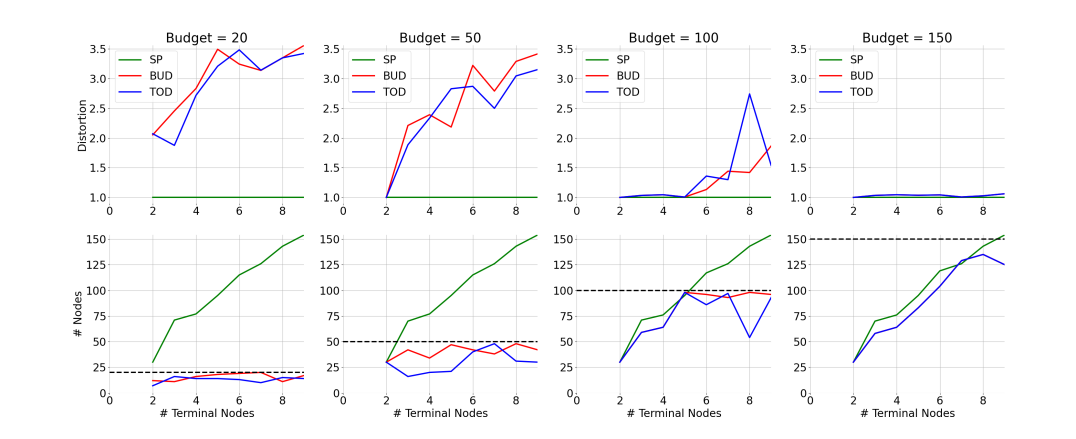
Figure 6: Comparison on distortion (top row) and number of nodes after compression (bottom row) for BUD-Lite and TOD-Lite against computing the shortest paths (SP) and pruning all nodes that are not on them. The dotted lines mark the communication budget.

V-B Results and Discussion

Comparison with baselines. The results on the four scenarios are documented in Table I. We show the compression time (label: “Comp”), the nominal (label: “Nom”, computed from the compressed DSG) and simulated (label: “Mis”, computed as the actual time $r_{1}$ takes to reach its destination in the simulator) mission times, and the size of the compressed DSG (upper bounded by the budget $B$), all averaged across three runs. The two best results for each row are in bold.

The combinatorial nature of problem (2) makes the ILP solver impractical in robotic applications: for the long runs, the calculation of Optimum did not finish within an hour.

In all scenarios, robot $r_{1}$ reaches the goal using the compressed DSG output by D-Lite. The simulated mission time is at times faster on the compressed graph compared to the full DSG because the former has fewer waypoints: a sparser list of waypoints in a less cluttered space can actually yield faster navigation. The different performance of BUD-Lite and TOD-Lite is due to the different abstraction mechanisms, whereby the path-wise node compression in the former yields finer granularity and usually better performance. Discrepancies between nominal and simulated mission times are due to local navigation, whose exploration time is difficult to estimate a posteriori from the full DSG. D-Lite always outperforms IB in terms of both nominal and simulated mission times. Specifically, the navigation planned on the compressed DSG produced by BUD-Lite is only a minute longer than the optimal path on the original DSG. IB is also unable to find a compressed DSG that preserves the necessary connectivity for the long1 case.

Ablation study. We compare distortion and number of nodes on the shortest paths between terminal nodes, for increasing number of terminal nodes and increasing budget constraints in Fig. 6. The shortest paths are optimal in terms of navigation performance (no distortion, top row), but easily violate the communication constraints (exceeding the budget, bottom row). On the other hand, BUD-Lite and TOD-Lite trade-off the path lengths between the terminal nodes to meet the budget constraint, and as we relax the latter, the distortion decreases. For the case with a budget of 150 nodes (last column), BUD-Lite and TOD-Lite obtain the same results, since the initial spanner already satisfies the budget constraint.

Figure 7 shows an ablation on the compression time along with the number of nodes removed or added from the initial spanner for different budget sizes and with an increasing number of terminal nodes. We observe that the compression time is still reasonable in practice (in the order of seconds) even with up to 50 terminal nodes and compressing the DSG to less than 5% of its original size. The runtime of the compression algorithms is dominated by the initial spanner construction in build_spanner.

Figure 8 plots the maximal distortion against the theoretical bounds proposed in 1. While the tightness of the bounds varies, it still gives a useful estimate of the worst-case distortion. In particular, we note that the bound is typically tighter for larger numbers of terminal nodes and lower budget.

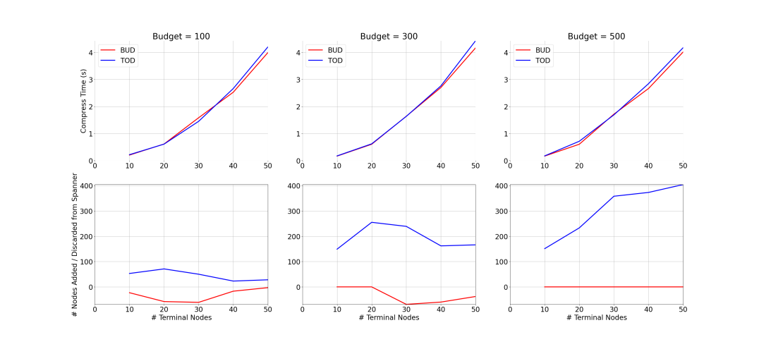
Figure 7: First row shows the compression time for a DSG with 3814 nodes for different number of terminals and budgets; second row shows the corresponding number of nodes removed (when abstracting nodes for BUD) or added (when expanding nodes for TOD). The overall compression time is dominated by the construction of the spanner.

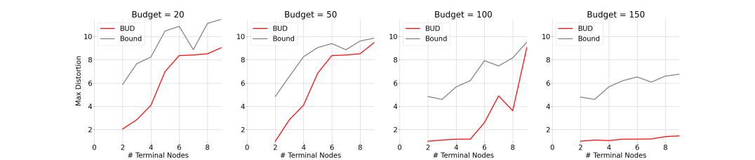
Figure 8: We show the distortion implied by the bound in Proposition 1 compared with the maximum distortion from the result of BUD-Lite for varying budgets and number of terminals using the DSG of the Office environment with 3814 nodes.

VI Conclusions

Motivated by the goal of enabling efficient information sharing for robots that collaboratively explore an unknown environment, we have proposed algorithms to suitably compress 3D Scene Graphs built and transmitted by robots during exploration, for the case when resource constraints of a shared communication channel make lossless transmission infeasible. Our algorithms can accommodate the presence of a sharp budget on the size of the transmitted map, run in real time, and perform graph compression with attention to the performance on specified navigation tasks. Simulated experiments carried out with a realistic simulator show that our approach is able to meet communication constraints while providing satisfactory performance of navigation tasks planned on the compressed DSG.

The proposed approach opens several interesting avenues for future work. In fact, 3D Scene Graphs are recently developed tools, and their use in multi-robot cooperation and collaboration is still relatively unexplored. For example, it is interesting to adapt our compression algorithms to data collection in dynamic environments —as the ones considered in [54]— that induce time-varying graphs. Also, extension of compression techniques to various and more general tasks should be addressed. Finally, validation of the proposed algorithms on real robots is desired to test their impact in the real world.

Appendix A Exact Budget-Constrained Spanner

Problem (2) can be solved exactly by the following ILP (adapted from the exact spanner formulation in [48, Section 4]), x_i  ∀i∈V_Gx_i,j^st ∀(i,j)∈E_G,∀(s,t)∈Pβ ∑_(i,j) ∈¯E__G x_(i,j)^u v W^G(i,j) ≤d_G(s,t) + βW_max^G(s,t) ∀(s,t)∈P, ∀(i,j)∈E_G ∑_(i,j) ∈Out(i) x_(i,j)^st-∑_(j,i) ∈In(i) x_(j,i)^st = {1 i=s-1 i=t0 else ∀(s,t)∈P, ∀i ∈V_G ∑_(i,j) ∈Out(i) x_(i,j)^st ≤1 ∀(s,t)∈P, ∀i ∈V_G x_i≥x_(i,j)^st + x_(j,i)^st ∀(s,t)∈P, ∀i ∈V_G,∀(i,j)∈E_G ∑_i∈V_G x_i≤B x_i,x_(i,j)^st∈{0,1} ∀(s,t)∈P, ∀i ∈V_G, ∀(i,j)∈E_G, where $x_{i}$ is associated with each node $i\in\mathcal{V}_{\mathcal{G}}$ and is $1$ if it is included in the spanner, $x_{(i,j)}^{st}$ is an edge variable equal to $1$ if and only if edge $(i,j)$ is taken as part of the path between $s$ and $t$, $\overline{\mathcal{\mathcal{E}}}_{\mathcal{G}}$ is the augmented set of bidirected edges, obtained by adding edge $(j,i)$ for each edge $(i,j)\in\mathcal{E}_{\mathcal{G}}$, (A) forces maximum distortion for all paths between terminal nodes, (A)–(A) ensure that the chosen edges form a path for each pair of terminals $(s,t)$, (A) ensures that a node $i$ is taken if any edges incident to it are taken, and (A) encodes the limited budget on the number of selected nodes.

Appendix B calculation of edge weights

The edge weights associated with the intra-layer edges of the 3D Scene Graph $\mathcal{G}$ are simply the Euclidean distance between the two nodes the edge connects. For example, for the layer consisting of places, the weight associated to an edge would be the Euclidean distance between the two connected places; for the layer consisting of rooms, the edge weight would be the Euclidean distance between the centroid of two rooms. The calculation of inter-layer edge weights is more nuanced: they cannot be simply Euclidean distances, since that would fail to capture the actual effort to traverse, for example, from a room centroid to a place in the room without precise knowledge of free-space locations in the place layer. Intuitively, the lack of such precise spatial information requires the robot to parse the room by locally exploring it, until the target location (place) is reached. In general, if the robot is aware only of an abstract, spatially coarse representation of granular geometric information about free-space locations (such as a room or building node that represents a set of places nodes), time-consuming exploration is needed to supply the missing spatial information. This fact well summarizes the trade-off that a robot faces when compressing its local map: high compression rate enables quicker transmission, but inevitably causes the robot that receives the compressed map to perform suboptimal navigation.

Hence, for inter-layer edges, we devise a method to associate to each edge a weight that is at least as large as the shortest path of traversal. In particular, for each inter-layer edge, we have a node in the higher layer, denoted by $\mathbf{x}$, and a node in the lower layer, denoted by $\mathbf{y}$. To find the weight of the inter-layer edge $e_{\mathbf{x},\mathbf{y}}$ connecting $\mathbf{x}$ and $\mathbf{y}$, we first find a node $\mathbf{y}_{0}$ in the lower layer that has the smallest Euclidean norm to the centroid of the set of all the nodes that are children of $\mathbf{x}$: then, the weight of $e_{\mathbf{x},\mathbf{y}}$ is computed as

$$W^{\mathcal{G}}(\mathbf{x},\mathbf{y})\doteq\lVert\mathbf{x}-\mathbf{y}_{0}\rVert+d_{\mathcal{G}}(\mathbf{y}_{0},\mathbf{y}),$$ (11)

where $\lVert\cdot\rVert$ denotes the Euclidean norm. Observe that the weight is greater than or equal to the path length of the shortest path between $\mathbf{y}_{0}$ and $\mathbf{y}$. Intuitively, the weight of a room-to-place inter-layer edge is the distance between the room centroid and the closest place, plus the path length from the closest place to the target place.

Importantly, the above heuristic is consistent with navigation performance: the cost (i.e., estimated navigation time) of traversing the inter-layer edge between two nodes (e.g., to navigate from a place node to the room centroid) is higher than following the shortest path on the place layer that connects the two corresponding place nodes (e.g., the source place node and the closest place node to the room centroid). This feature is crucial in order for the proposed compression algorithms to work properly, because they will first favor intra-layer edges (which retain navigation performance) and use inter-layer edges only when necessary (causing an increase in navigation time).

However, we also note that calculating the actual impact of local navigation is difficult having only the final DSG, so that the actual navigation time may differ from the estimated one. Nonetheless, we argue that such inter-layer edge weights could be reliably estimated by a robot navigating the environment. Indeed, rather than calculating the weights a posteriori based on the final DSG, the robot can compute them online (while building the DSG) based on its own exploration time: this directly relates inter-layer edges between places, rooms, and buildings nodes with the expected navigation effort.

Appendix C Proof of 1

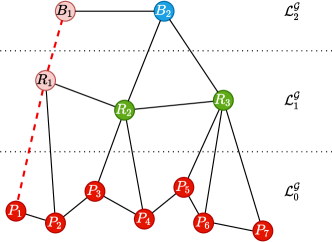
Figure 9: Partition of a toy 3D Scene Graph into layers. The ancestors of place node $P_{1}$ are colored in light red and connected through dashed red edges. For example, room node $R_{1}$ is the $1$st ancestor of $P_{1}$, that is, $a_{1}^{\mathcal{G}}(P_{1})=R_{1}$. The three rooms have diameter equal to $2$, $2$, and $3$, respectively. For example, $\mathrm{diam}_{\mathcal{G}}(R_{3})=3$ because $P_{5}$ and $P_{7}$, which are the nodes farthest apart among all its children, are connected by the shortest path $\{P_{5},P_{6},P_{7}\}$ with cardinality $3$.

Proof.

First, recall that terminals are place nodes, that is, for any $(s,t)\in\mathcal{P}$, it holds $s,t\in\mathcal{L}_{0}^{\mathcal{G}}$.

Algorithm 2 first builds a spanner with maximum distortion parameterized by $\beta$. Hence, the finest layer (with the smallest index) retained in such initial spanner needs to be either $\mathcal{L}_{\ell_{0}}^{\mathcal{G}}$, with $\ell_{0}$ defined above, or any layer below. In particular, retaining $\mathcal{L}_{\ell_{0}}^{\mathcal{G}}$ as the finest layer yields the maximum tolerable distortion given $\beta$. This can be seen from the following inequalities valid for any path $P_{\mathcal{G}^{\prime}}(s,t)$ whose nodes are in layer $\mathcal{L}_{\ell}^{\mathcal{G}}$ or in layers above:

$$d_{\mathcal{G}^{\prime}}(s,t)\geq 2\sum_{i=1}^{\ell}W_{\text{min}}^{i-1,i}+u_{\text{min}}^{\ell}W_{\text{min}}^{\ell}$$ (12)

where the summation accounts for cross-layer edges connecting nodes $s$ and $t$ to their respective ancestors in layer $\mathcal{L}_{\ell}^{\mathcal{G}}$ and the term $u_{\text{min}}^{\ell}W_{\text{min}}^{\ell}$ accounts for the minimum distance between such two ancestors. Then, after creation of the initial spanner, there exists at least one pair $(s,t)\in\mathcal{P}$ whose shortest path $P_{\mathcal{G}^{\prime}}(s,t)$ passes across layer $\mathcal{L}_{\ell_{0}}^{\mathcal{G}}$ or a layer below. Because the spanner construction is near-optimal and only guarantees an upper bound on distance stretch, it is possible that finer layers (with index smaller than $\ell_{0}$) are retained, providing lower distortion for shortest paths passing across them.

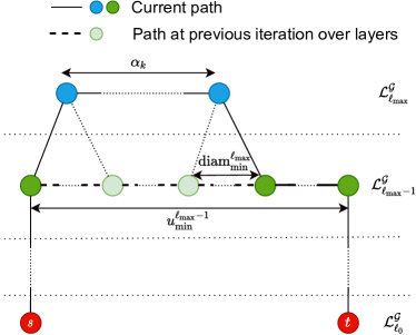
Figure 10: Representation of the maximum distortion provided by a shortest path in the compressed graph. Terminal pair $(s,t)\in\mathcal{P}$ is in the finest layer $\mathcal{L}_{\ell_{0}}^{\mathcal{G}}$ retained by the spanner, which here corresponds to the place layer. After $k$ total iterations, the path has at most $\alpha_{k}$ nodes in the highest layer $\mathcal{L}_{\ell_{\text{max}}}^{\mathcal{G}}$. The remaining nodes in layer $\mathcal{L}_{\ell_{\text{max}}-1}^{\mathcal{G}}$ are at most the ones that remain after replacement of at least $\mathrm{diam}_{\text{min}}^{\ell_{\text{max}}}$ nodes for each newly added node in layer $\mathcal{L}_{\ell_{\text{max}}}^{\mathcal{G}}$.

Consider now any number $k$ of total iterations of the innermost loop of Algorithm 2 at Algorithm 2 that parses terminal pairs. After $\ell$ layers have been parsed in the outmost loop at Algorithm 2, with the last layer $\mathcal{L}_{\ell}^{\mathcal{G}}$ having possibly been parsed only partially, the total number of iterations is lower bounded as follows:

$$k>|\mathcal{P}|\sum_{i=\ell_{0}}^{\ell-1}u_{\text{min}}^{i}$$ (13)

where each pair has been parsed for at least $\sum_{i=\ell_{0}}^{\ell-1}u_{\text{min}}^{i}$ iterations to reach the $\ell$th layer. In particular, each pair is parsed for at least $u_{\text{min}}^{i}$ iterations in the innermost loop for each layer $\mathcal{L}_{i}^{\mathcal{G}}$, $i=\ell_{0},\dots,\ell-1$, plus other possible iterations for layer $\mathcal{L}_{\ell}^{\mathcal{G}}$. Then, the highest layer $\mathcal{L}_{\ell}^{\mathcal{G}}$ that can be reached after $k$ total iterations has index $\ell=\ell_{\text{max}}$ defined above. Because higher layers feature coarser spatial resolution, the maximum distortion is given by the path with the largest distortion that passes across the highest reachable layer $\ell_{\text{max}}$. This finally yields the upper bound in (4), as described next. The summation is the maximum distance given by cross-layer edges that connect terminals $s$ and $t$ to layer $\mathcal{L}_{\ell_{\text{max}}}^{\mathcal{G}}$. The maximum number of steps (nodes) of any path in such a layer is given by $\alpha_{k}$ defined above, whereby each layer $\mathcal{L}_{i}^{\mathcal{G}}$ below $\mathcal{L}_{\ell_{\text{max}}}^{\mathcal{G}}$ provides the least number of steps between the corresponding $i$th ancestors of $s$ and $t$. Thus, the term $\alpha_{k}W_{\text{max}}^{\ell_{\text{max}}}$ is the maximum length of the portion of the path in layer $\mathcal{L}_{\ell_{\text{max}}}^{\mathcal{G}}$. Finally, the last term is the maximum length of the remaining portion of the path, which passes across nodes in layer $\mathcal{L}_{\ell_{\text{max}}-1}^{\mathcal{G}}$ by construction. In particular, the maximum number of steps is given by $u_{\text{min}}^{\ell_{\text{max}}-1}-\alpha_{k}\mathrm{diam}_{\text{min}}^{\ell_{\text{max}}}$, that accounts for the remaining number of edges in layer $\mathcal{L}_{\ell_{\text{max}}-1}^{\mathcal{G}}$ after $\alpha_{k}$ iterations on the $\ell_{\text{max}}$th layer. ∎

Appendix D Extra Numerical Tests and Simulations Results

In this Appendix, we visually illustrate how the proposed algorithms perform on two tested simulated environments: an apartment scene and the office scene already used in Section V.

D-A Apartment Scene

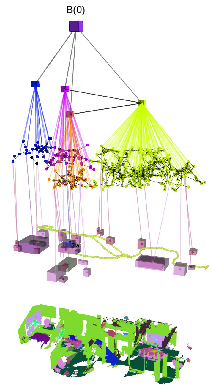
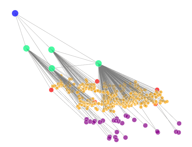
Figure 11: Original 3D Scene Graph of the Apartment scene. Left: full DSG with semantic map and meshgrid. Right: schematic version with objects (purple), places (yellow), rooms (green), and building (blue) nodes. Terminal places nodes are marked with red color. Full size: $453$ nodes.

Figure 11 shows the original DSG of the Apartment, which is composed of $453$ nodes connected by $1403$ edges.

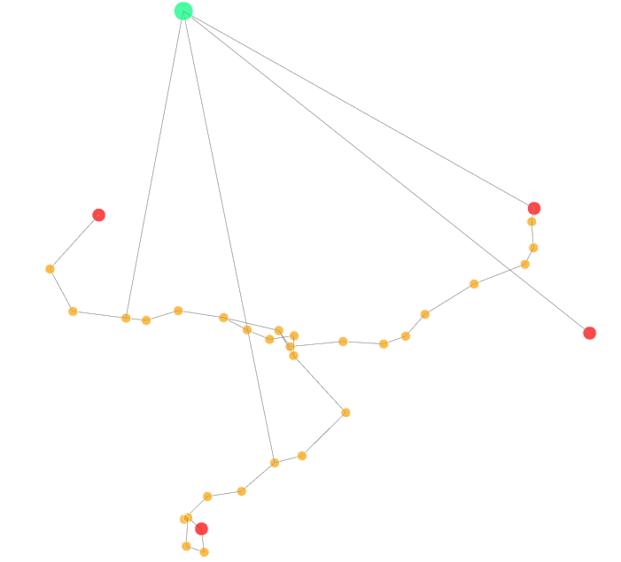
((a)) Budget: $40$ nodes (actual size: $34$).

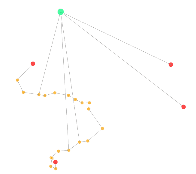
((b)) Budget: $30$ nodes (actual size: $24$).

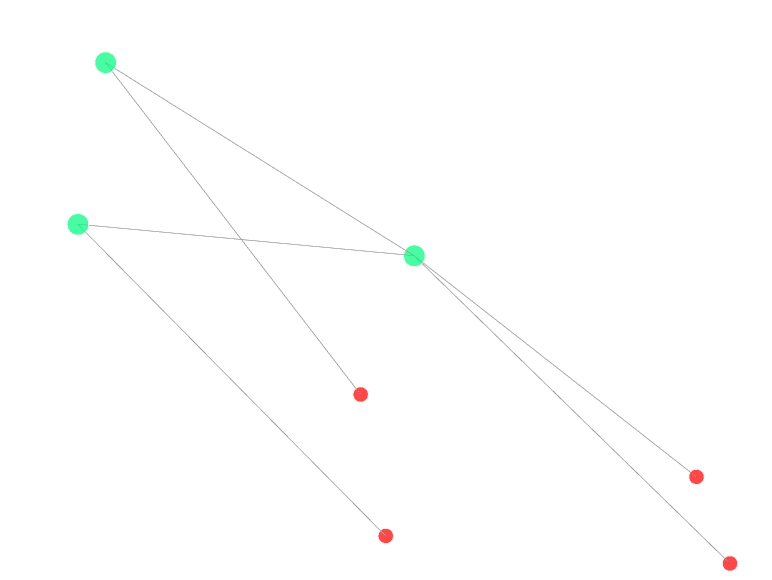
((c)) Budget: $10$ nodes (actual size: $7$).

Figure 12: Compressed 3D Scene Graph of the Apartment output by BUD-Lite.

Figure 12 shows the compressed graphs obtained by running BUD-Lite with different budget values. Recall that BUD-Lite compressed the DSG by exploiting the hierarchy bottom-up, parsing shortest paths one after the other and abstracting away places nodes to their corresponding room nodes. In this case, we consider four terminals nodes scattered across three rooms. Note that, as the available budget decreases (i.e., the communication constraint get tighter), portions of shortest paths along places nodes are pruned away and abstracted into their respective room nodes. In particular, BUD-Lite uses a single room node when the budget is $30$ (12(a)) or larger (12(b)), sacrificing navigation performance for the two terminals nodes belonging to that room and retaining fine-scale spatial information in proximity of the two terminals nodes belonging to other two rooms. Conversely, all rooms are used when the budget gets too small (12(c)), and the compression procedure is forced to remove all free-space locations in the place layer. Importantly, the output of BUD-Lite also depends on the order in which terminals pairs (and hence shortest paths) are parsed, which may cause larger or smaller amounts of nodes to be deleted before others: improving this feature of the algorithm is an important aspect that will be considered in follow-up work.

((a)) Budget: $40$ nodes (actual size: $13$).

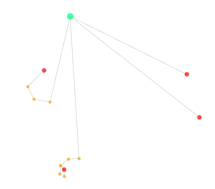
((b)) Budget: $30$ nodes (actual size: $13$).

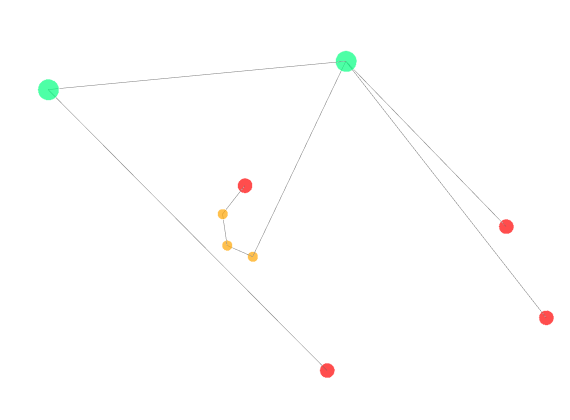
((c)) Budget: $10$ nodes (actual size: $9$).

Figure 13: Compressed 3D Scene Graph of the Apartment output by TOD-Lite.

Conversely, TOD-Lite results are shown in Fig. 13. Recall that this algorithm leverages the DSG hierarchy via top-down expansion of nodes, which is clearly visible from Fig. 13 as opposed to shortest path-wise compression on BUD-Lite. In particular, it can be seen from Figs. 13(a) and 13(b) that expanding one room node is not possible without exceeding the allowed budget: hence, TOD-Lite expands the other two rooms nodes in both cases, resulting in preserved places nodes close to the two terminals nodes on the left. When budget is further reduced (13(c)), two rooms are not expanded and fine-scale geometric information in the place layer is retained only for the room corresponding to the terminal node on the top left.

Comparing the compression results of BUD-Lite in Fig. 12 and of TOD-Lite in Fig. 13 shows both their different mechanisms and advantages: in this case, large budgets favor the BUD-Lite bottom-up compression, which is able to retain more places nodes; instead, small budget favors the TOD-Lite top-down expansion, which eventually retains places nodes associated with one room, whereas the order chosen to parse shortest paths in the BUD-Lite forces to abstract away all nodes in the place layer.

D-B Office Scene

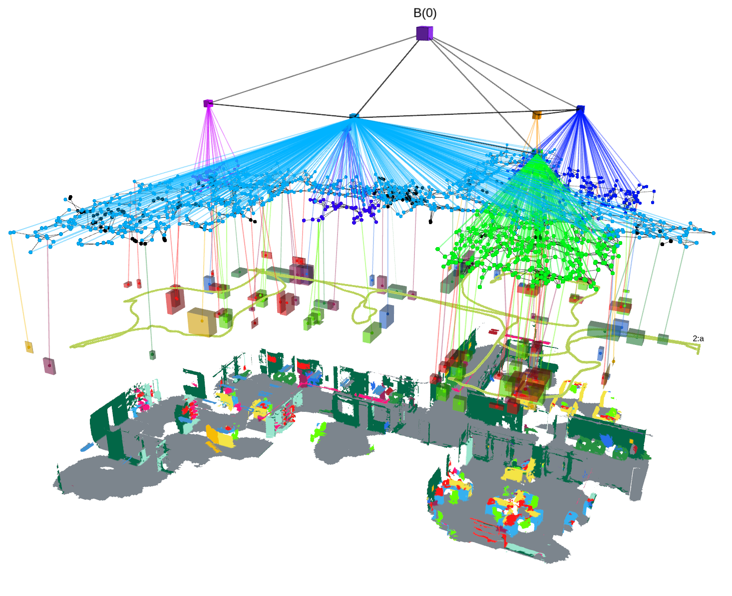
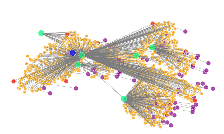
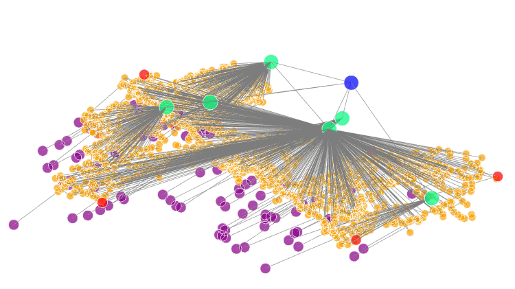
Figure 14: Original 3D Scene Graph of the Office scene. Left: full DSG with semantic map and meshgrid. Right: schematic version. Full size: $1675$ nodes.

Figure 14 shows the original DSG of the Office, which is composed of $1675$ nodes connected by $5396$ edges. For this test, we consider six terminal nodes scattered across two rooms.

((a)) Budget: $60$ nodes (actual size: $55$).

((b)) Budget: $30$ nodes (actual size: $24$).

((c)) Budget: $10$ nodes (actual size: $8$).

Figure 15: Compressed 3D Scene Graph of the Office output by BUD-Lite.

Figure 15 shows the compressed graphs output by BUD-Lite. The same general remarks carried out before also apply here. Notably, one of the interested rooms (gathering five out of the six terminals nodes) is very large (it is in fact a corridor, see Fig. 14), which may cause the compression procedure of BUD-Lite to act in too unbalanced fashion if the portions of shortest paths passing through that room are abstracted away at once. To improve granularity of compression in this case, we forced a maximum number of places nodes that can be compressed within a single iteration (corresponding to a slight modification to the condition of Algorithm 2 of Algorithm 2): in particular, we set $20$ places nodes as maximum threshold, so that long stretches of places nodes are compressed at a pace of $20$ (or fewer) at each iteration.

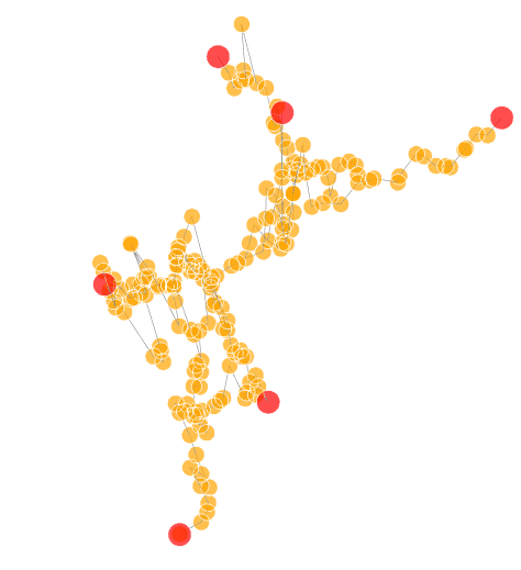
((a)) Initial condition.

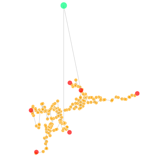
((b)) Iteration $1$.

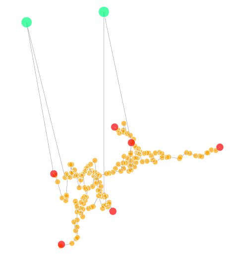
((c)) Iteration $2$.

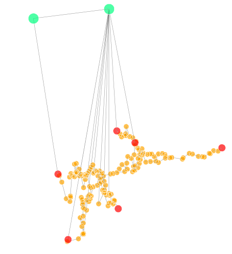
((d)) Iteration $10$.

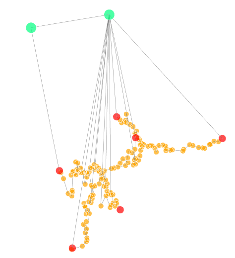
((e)) Iteration $11$.

((f)) Iteration $15$.

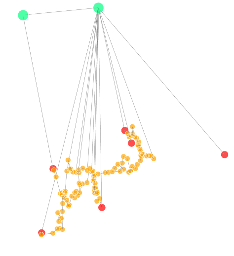
((g)) Iteration $20$.

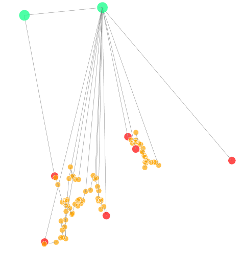
((h)) Iteration $25$.

Figure 16: Iterations of the bottom-up compression phase of BUD-Lite (budget: $60$ nodes).

Figure 16 shows the breakdown of some iterations of the compression procedure carried out within the BUD-Lite algorithm, corresponding to the loop at Algorithm 2 of Algorithm 2. The initial condition shown in 16(a) corresponds to the spanner output by build_spanner in Algorithm 2. Note that the latter is composed of only places nodes, and rooms nodes abstractions are introduced by subsequent compression iterations. Specifically, one room is added at the first iteration (16(b)) and the other, which is connected to the first room, at the second iteration (16(c)). Shortest paths are parsed one after the other, which causes places nodes to be retained until there is no path using them: for example, the inter-layer edge between the rightmost terminal node and its associated room node is added at iteration $11$ (16(e)), but the corresponding stretch of places nodes is removed only at iteration $15$ (16(f)), when all shortest paths with source the rightmost terminal node have been parsed and shortcut through the room. The output compressed DSG in 15(a) is obtained after $28$ iterations.

((a)) Budget: $60$ nodes (actual size: $38$).

((b)) Budget: $30$ nodes (actual size: $22$).

((c)) Budget: $10$ nodes (actual size: $9$).

Figure 17: Compressed 3D Scene Graph of the Office output by TOD-Lite.

Figure 17 shows the compressed graphs output by TOD-Lite. The same general remarks carried out for the Apartment also apply here. In particular, note that the small budget of $10$ nodes in this case prevents TOD-Lite to perform any expansion, see 17(c).

References

- [1] A. Rosinol, A. Gupta, M. Abate, J. Shi, and L. Carlone, “3D dynamic scene graphs: Actionable spatial perception with places, objects, and humans,” in Robotics: Science and Systems (RSS), 2020, (pdf), (media), (video). [Online]. Available: http://news.mit.edu/2020/robots-spatial-perception-0715
- [2] N. Hughes, Y. Chang, and L. Carlone, “Hydra: a real-time spatial perception engine for 3D scene graph construction and optimization,” in Robotics: Science and Systems (RSS), 2022, (pdf).
- [3] I. Armeni, Z. He, J. Gwak, A. Zamir, M. Fischer, J. Malik, and S. Savarese, “3D scene graph: A structure for unified semantics, 3D space, and camera,” in Intl. Conf. on Computer Vision (ICCV), 2019, pp. 5664–5673.
- [4] S. Wu, J. Wald, K. Tateno, N. Navab, and F. Tombari, “SceneGraphFusion: Incremental 3D scene graph prediction from RGB-D sequences,” in IEEE Conf. on Computer Vision and Pattern Recognition (CVPR), 2021.
- [5] U. Kim, J. Park, T. Song, and J. Kim, “3-D scene graph: A sparse and semantic representation of physical environments for intelligent agents,” IEEE Trans. Cybern., vol. PP, pp. 1–13, Aug. 2019.
- [6] R. Talak, S. Hu, L. Peng, and L. Carlone, “Neural trees for learning on graphs,” in Conf. on Neural Information Processing Systems (NeurIPS), 2021, (pdf).
- [7] T. Cieslewski, S. Choudhary, and D. Scaramuzza, “Data-efficient decentralized visual SLAM,” IEEE Intl. Conf. on Robotics and Automation (ICRA), 2018.
- [8] Y. Tian, K. Khosoussi, M. Giamou, J. P. How, and J. Kelly, “Near-optimal budgeted data exchange for distributed loop closure detection,” in Robotics: Science and Systems (RSS), 2018.
- [9] Y. Chang, Y. Tian, J. How, and L. Carlone, “Kimera-Multi: a system for distributed multi-robot metric-semantic simultaneous localization and mapping,” in IEEE Intl. Conf. on Robotics and Automation (ICRA), 2021, arXiv preprint arXiv: 2011.04087, (pdf).
- [10] C. Denniston, Y. Chang, A. Reinke, K. Ebadi, G. Sukhatme, L. Carlone, B. Morrell, and A. Agha-mohammadi, “Loop closure prioritization for efficient and scalable multi-robot SLAM,” IEEE Robotics and Automation Letters (RA-L), 2022, (pdf).
- [11] S. Choudhary, L. Carlone, C. Nieto, J. Rogers, H. Christensen, and F. Dellaert, “Distributed mapping with privacy and communication constraints: Lightweight algorithms and object-based models,” Intl. J. of Robotics Research, 2017, arxiv preprint: 1702.03435, (pdf) (web) (code) (code) (code) (video) (video) (video) (video).
- [12] A. Becker, P. N. Klein, and D. Saulpic, “A Quasi-Polynomial-Time Approximation Scheme for Vehicle Routing on Planar and Bounded-Genus Graphs,” in Proc. of the Annual European Symp. on Algorithms (ESA), vol. 87, 2017, pp. 12:1–12:15.
- [13] A. Dobson and K. E. Bekris, “Sparse roadmap spanners for asymptotically near-optimal motion planning,” Intl. J. of Robotics Research, vol. 33, no. 1, pp. 18–47, Jan. 2014.
- [14] A. C. Gilbert, T. Labs-Research, P. Avenue, F. Park, and K. Levchenko, “Compressing Network Graphs,” Proc. of the LinkKDD workshop at the ACM Conference on KDD, vol. 124, p. 10, 2004.
- [15] R. L. de Queiroz and P. A. Chou, “Compression of 3D Point Clouds Using a Region-Adaptive Hierarchical Transform,” IEEE Trans. on Image Processing, vol. 25, no. 8, pp. 3947–3956, Aug. 2016.
- [16] X. Sun, H. Ma, Y. Sun, and M. Liu, “A novel point cloud compression algorithm based on clustering,” IEEE Robotics and Automation Letters, vol. 4, no. 2, pp. 2132–2139, 2019.
- [17] D. Thanou, P. A. Chou, and P. Frossard, “Graph-based compression of dynamic 3d point cloud sequences,” IEEE Transactions on Image Processing, vol. 25, no. 4, pp. 1765–1778, 2016.
- [18] S. Raghavan and H. Garcia-Molina, “Representing Web graphs,” in Proc. International Conference on Data Engineering (Cat. No.03CH37405), Mar. 2003, pp. 405–416.
- [19] C. Chekuri, T. Rukkanchanunt, and C. Xu, “On Element-Connectivity Preserving Graph Simplification,” in Algorithms - ESA 2015, Berlin, Heidelberg, 2015, pp. 313–324.
- [20] P. Harish, P. J. Narayanan, V. Vineet, and S. Patidar, “Chapter 7 - Fast Minimum Spanning Tree Computation,” in GPU Computing Gems Jade Edition, ser. Applications of GPU Computing Series, Jan. 2012, pp. 77–88.
- [21] K. Mehlhorn, “A faster approximation algorithm for the Steiner problem in graphs,” Information Processing Letters, vol. 27, no. 3, pp. 125–128, Mar. 1988.
- [22] R. Ahmed, G. Bodwin, F. D. Sahneh, K. Hamm, M. J. L. Jebelli, S. Kobourov, and R. Spence, “Graph spanners: A tutorial review,” Computer Science Review, vol. 37, p. 100253, Aug. 2020.
- [23] Y. Kobayashi, “An FPT Algorithm for Minimum Additive Spanner Problem,” in International Symposium on Theoretical Aspects of Computer Science (STACS), vol. 154, 2020, pp. 11:1–11:16.
- [24] M. Elkin, Y. Gitlitz, and O. Neiman, “Improved weighted additive spanners,” Distrib. Comput., Aug. 2022.
- [25] G. Bodwin, “On the Structure of Unique Shortest Paths in Graphs,” in Proc. of the Annual ACM-SIAM Symp. on Discrete Algorithms (SODA), Jan. 2019, pp. 2071–2089.
- [26] M. Elkin and O. Neiman, “Efficient Algorithms for Constructing Very Sparse Spanners and Emulators,” ACM Trans. Algorithms, vol. 15, no. 1, pp. 4:1–4:29, Nov. 2018.
- [27] U. Kang and C. Faloutsos, “Beyond ’Caveman Communities’: Hubs and Spokes for Graph Compression and Mining,” in Proc. of the IEEE International Conference on Data Mining, Dec. 2011, pp. 300–309.
- [28] M. Besta and T. Hoefler, “Survey and Taxonomy of Lossless Graph Compression and Space-Efficient Graph Representations,” arXiv:1806.01799 [cs, math], Apr. 2019.
- [29] A. Borici and A. Thomo, “Semantic Graph Compression with Hypergraphs,” in IEEE International Conference on Advanced Information Networking and Applications, Victoria, BC, Canada, May 2014, pp. 1097–1104.
- [30] J.-G. Young, G. Petri, and T. P. Peixoto, “Hypergraph reconstruction from network data,” Commun. Phys., vol. 4, no. 1, p. 135, Dec. 2021.
- [31] G. Karypis and V. Kumar, “Multilevel k-Way Hypergraph Partitioning,” in Design Automation Conference, Jun. 1999, pp. 343–348.
- [32] K. Devine, E. Boman, R. Heaphy, R. Bisseling, and U. Catalyurek, “Parallel hypergraph partitioning for scientific computing,” in Proc. of the IEEE International Parallel & Distributed Processing Symposium, 2006, p. 10 pp.
- [33] S. Zhang, Z. Ding, and S. Cui, “Introducing Hypergraph Signal Processing: Theoretical Foundation and Practical Applications,” IEEE Internet Things J., vol. 7, no. 1, pp. 639–660, Jan. 2020.
- [34] T. Silver, R. Chitnis, A. Curtis, J. B. Tenenbaum, T. Lozano-Pérez, and L. P. Kaelbling, “Planning with Learned Object Importance in Large Problem Instances using Graph Neural Networks,” Proc. of the AAAI Conference on Artificial Intelligence, vol. 35, no. 13, pp. 11 962–11 971, May 2021.
- [35] C. Agia, K. M. Jatavallabhula, M. Khodeir, O. Miksik, V. Vineet, M. Mukadam, L. Paull, and F. Shkurti, “Taskography: Evaluating robot task planning over large 3D scene graphs,” in Conference on Robot Learning (CoRL). PMLR, Jan. 2022, pp. 46–58.
- [36] Y. Tian, K. Khosoussi, and J. P. How, “A resource-aware approach to collaborative loop-closure detection with provable performance guarantees,” Intl. J. of Robotics Research, vol. 40, no. 10-11, pp. 1212–1233, Sep. 2021.
- [37] D. T. Larsson, D. Maity, and P. Tsiotras, “Q-Tree Search: An Information-Theoretic Approach Toward Hierarchical Abstractions for Agents With Computational Limitations,” IEEE Trans. Robotics, vol. 36, no. 6, pp. 1669–1685, Dec. 2020.
- [38] ——, “Information-theoretic abstractions for resource-constrained agents via mixed-integer linear programming,” in Proc. of the Workshop on Computation-Aware Algorithmic Design for Cyber-Physical Systems, May 2021, pp. 1–6.
- [39] ——, “Information-Theoretic Abstractions for Planning in Agents With Computational Constraints,” IEEE Robotics and Automation Letters, vol. 6, no. 4, pp. 7651–7658, Oct. 2021.
- [40] P. N. Klein, “A subset spanner for Planar graphs, with application to subset TSP,” in Proceedings of the Annual ACM Symposium on Theory of Computing, ser. STOC ’06, May 2006, pp. 749–756.
- [41] I. Althöfer, G. Das, D. Dobkin, D. Joseph, and J. Soares, “On sparse spanners of weighted graphs,” Discrete Comput Geom, vol. 9, no. 1, pp. 81–100, Jan. 1993.
- [42] T. Kavitha, “New Pairwise Spanners,” in International Symposium on Theoretical Aspects of Computer Science (STACS 2015), vol. 30, 2015, pp. 513–526.
- [43] S. Baswana, T. Kavitha, K. Mehlhorn, and S. Pettie, “Additive spanners and (a,b)-spanners,” ACM Trans. Algorithms, vol. 7, no. 1, pp. 5:1–5:26, Dec. 2010.
- [44] A. Abboud and G. Bodwin, “The 4/3 Additive Spanner Exponent Is Tight,” J. ACM, vol. 64, no. 4, pp. 28:1–28:20, Sep. 2017.
- [45] M. Cygan, F. Grandoni, and T. Kavitha, “On Pairwise Spanners,” in International Symposium on Theoretical Aspects of Computer Science (STACS), vol. 20, Dagstuhl, Germany, 2013, pp. 209–220.
- [46] M. Elkin, Y. Gitlitz, and O. Neiman, “Almost Shortest Paths with Near-Additive Error in Weighted Graphs,” in Proc. of the Scandinavian Symposium and Workshops on Algorithm Theory (SWAT), vol. 227, 2022, pp. 23:1–23:22.
- [47] R. Ahmed, G. Bodwin, F. D. Sahneh, S. Kobourov, and R. Spence, “Weighted Additive Spanners,” in Graph-Theoretic Concepts in Computer Science, ser. Lecture Notes in Computer Science, 2020, pp. 401–413.
- [48] R. Ahmed, G. Bodwin, F. D. Sahneh, K. Hamm, S. Kobourov, and R. Spence, “Multi-Level Weighted Additive Spanners,” in Proc. of the International Symposium on Experimental Algorithms (SEA), vol. 190, 2021, pp. 16:1–16:23.
- [49] K. Censor-Hillel, T. Kavitha, A. Paz, and A. Yehudayoff, “Distributed construction of purely additive spanners,” Distrib. Comput., vol. 31, no. 3, pp. 223–240, Jun. 2018.
- [50] S. Baswana and S. Sarkar, “Fully dynamic algorithm for graph spanners with poly-logarithmic update time,” in Proc. of the Annual ACM-SIAM Symp. on Discrete Algorithms (SODA), Jan. 2008, pp. 1125–1134.
- [51] S. Arya, G. Dast, D. M. Mount, J. S. Salowe, and M. Smid, “Euclidean spanners: Short, thin, and lanky,” in Proc. of the Acm Symposium on Theory of Computing, 1995, pp. 489–498.
- [52] A. Abboud and G. Bodwin, “Reachability Preservers: New Extremal Bounds and Approximation Algorithms,” in Proc. of the Annual ACM-SIAM Symp. on Discrete Algorithms (SODA), Jan. 2018, pp. 1865–1883.
- [53] N. Tishby, F. Pereira, and W. Bialek, “The information bottleneck method,” Proc. of the Allerton Conference on Communication, Control and Computation, vol. 49, 07 2001.
- [54] A. Rosinol, A. Violette, M. Abate, N. Hughes, Y. Chang, J. Shi, A. Gupta, and L. Carlone, “Kimera: from SLAM to spatial perception with 3D dynamic scene graphs,” Intl. J. of Robotics Research, vol. 40, no. 12–14, pp. 1510–1546, 2021, arXiv preprint arXiv: 2101.06894, (pdf).