The BlueMUSE data reduction pipeline: lessons learned from MUSE and first design choices

Abstract

BlueMUSE is an integral field spectrograph in an early development stage for the ESO VLT. For our design of the data reduction software for this instrument, we are first reviewing capabilities and issues of the pipeline of the existing MUSE instrument. MUSE has been in operation at the VLT since 2014 and led to discoveries published in more than 600 refereed scientific papers. While BlueMUSE and MUSE have many common properties we briefly point out a few key differences between both instruments. We outline a first version of the flowchart for the science reduction, and discuss the necessary changes due to the blue wavelength range covered by BlueMUSE. We also detail specific new features, for example, how the pipeline and subsequent analysis will benefit from improved handling of the data covariance, and a more integrated approach to the line-spread function, as well as improvements regarding the wavelength calibration which is of extra importance in the blue optical range. We finally discuss how simulations of BlueMUSE datacubes are being implemented and how they will be used to prepare the science of the instrument.

1 INTRODUCTION

BlueMUSE is a new project that is building on the legacy of the successful MUSE instrument[1, 2] at the ESO VLT. It has just started the pre-design (“Phase A”) and is planned to be installed at one of the VLTs in 2030. The science cases to build this new instrument and its planned top-level parameters were already outlined in a White Paper[3].

Briefly, BlueMUSE will be a panoramic integral field spectrograph which is thought to cover at least $1\hbox{${}^{\prime}$}\times 1\hbox{${}^{\prime}$}$ on the sky with fine sampling of 0$.\!\!^{\prime\prime}$3/pix or better. It will cover the blue part of the optical spectrum, from the atmospheric cutoff at 350 nm to about 550 nm in one shot with high throughput. It will feature twice the spectral resolution of MUSE, i.e. $\left<R\right>\approx 3600$ when averaged over the wavelength range. Like MUSE, BlueMUSE will be made of 24 slicer-style integral field units and record the spectra on as many 4k$\times$4k CCDs. BlueMUSE will not, however, be coupled to an adaptive optics system, it will therefore operate with a single mode, with a stronger focus on instrument stability and even higher operational efficiency with minimal overheads.

Since both instruments have a very similar design, it makes sense to look at the successes and failures of the MUSE pipeline[4] (Sect. 2) before starting to design a pipeline for the new BlueMUSE instrument (in Sect. 3). We will discuss selected items of the new design in a bit more detail (Sect. 4) and present the basic ideas of the code to create simulated datacubes (Sect. 5).

2 MUSE PIPELINE: LESSONS LEARNED

The MUSE instrument and its pipeline was a great success. As of June 2022 about 625 refereed publications are at least partially based on its data. In 2021 MUSE enabled the most publications of any ESO instrument, surpassing even HARPS and UVES. In part, this success was due to a data reduction pipeline that could deliver science-ready datacubes with standard parameters for a large range of science topics, ranging from solar-system objects[5, 6], Galactic nebulae[7, 8] and clusters[9, 10], nearby[11, 12, 13] as well as high-redshift[14, 15] galaxies.

In fact, that the pipeline was ready to support already the first commissioning run in February 2014 was of great importance. It could at that time already run the full suite of reduction steps to produced a datacube with most of the instrument signature and atmospheric effects removed. This allowed the pipeline team to concentrate on the most visible deficiencies, like an inverted field of view, a complete rewrite of the skyflat handling and of the computation and application of the line-spread function. All this resulted in the first MUSE science papers[16, 17] getting written and submitted within a month of the science verification observations that they were based on.

2.1 Pipeline design

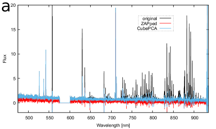
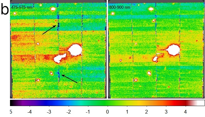
Figure 1: MUSE data issues. (a): HII region spectrum with pipeline sky subtraction (black), with additional ZAP cleaning (red), and processed with CubePCA (blue). While ZAP cleans the sky residuals, it also changes the continuum level. CubePCA leaves the continuum intact but also misses some of the telluric artifacts. (b): The picture shows images created by integrating one MUSE cube (containing a field with one bright star and a few small galaxies) over 100 nm at the blue and red end of the wavelength range. Each of the 24 IFUs is visible by a 12 pix high band across the field of view, the relative levels vary with wavelength. Arrows mark two strong dark features at the intersection of two slicer stacks.

However, a number of issues are still present in the pipeline and/or in the reduced data. For example, while the pipeline is parallelized in a large extent, only half of its processing is done with OpenMP parallelization while the other half essentially relies on the user starting multiple processes in parallel. This was an early design choice, imposed by the processing environment that was thought to be realized in about 2008 but was not present (any more) when the instrument was commissioned in 2014. This division resulted in a somewhat artificial split into “basic”- and “post”-processing which also made it necessary to save large files to disk in between. Effectively, this approach costs extra (temporary) diskspace and adds processing time (only $\sim\,3$%), but also complexity because the correct input files for the next step need to be determined (sometimes by user interaction).

2.2 Issues: sky subtraction

The most obvious issue with the data produced by the pipeline was related to the sky subtraction: the bright sky lines left unexpectedly large residuals. Various groups of MUSE users therefore developed separate packages to handle telluric emission lines better, ZAP[18], CubEx[19], and CubePCA[20], among the most prominent. This was especially necessary for science programs that took “deep” exposures of mostly empty sky regions which then tried to find faint line-emitting galaxies using automated methods[21, 22]. An additional complication for these extra procedures was that the exposure-combination algorithm implemented in the MUSE pipeline could no longer be used, since the extra sky-subtraction procedure worked only on resampled 3D cubes and not on the (unresampled) intermediate data. On the other hand, these extra processing steps could not be implemented in the pipeline itself, because they only work well, if most of the exposure is empty, which is only the case for a small fraction of the MUSE exposures, and because PCA-methods are hard to adapt to data that are not sampled on a regular grid, like intermediate MUSE data. Finally, while these extra sky-subtraction programs very efficiently suppress telluric residuals, they often change the data in unforeseen ways. An example can be seen in Fig. 1a where both extra processing steps remove the sky artifacts, but ZAP also removes the continuum of the HII region while CubePCA does not.

2.3 Issues: flat-fielding

The second obvious issue are patterns visible in images created from the reduced datacubes by integrating over many wavelength planes (Fig. 1b). MUSE is built from 24 individual slicer IFUs which cover the full width of the field. They visibly stand out in all exposures, and their pattern of dark and bright change with wavelength. On a smaller level, the four stacks of slices seem to create different patterns, especially between the two slicer stacks on the left and on the right of each IFU. Within each slicer stack, the images show an almost constant level. Finally, on the smallest scales, the horizontal intersections between the slicer stacks show a few especially dark (black arrows in Fig. 1b) and/or bright pixels.

While both issues, strong sky subtraction residuals and integrated image artifacts, are very different phenomena and their root cause is not finally understood, they are both strongly tied to the quality of flat-fielding. Indeed, several calibrations (line-spread function, wavelength calibration, OH-transition flux ratios, and line flux homogeneity) were tested as to their effects on the sky subtraction accuracy. It turned out that the fluxes are varying across the field at the $\sim\!$1.7% level, which is about the same level of variations seen in the sky background (as in Fig. 1b). The sky-line residuals visible in Fig. 1a are almost all less than 1% of the original flux of the line (this was shown to be true for most spectra[4]). The assumed flux ratios and the wavelengths of the telluric emission lines have systematic errors, too, but their effects are typically below this level.

Therefore, by improving the flux calibration across the field through better flat-fielding, one could also improve the accuracy of the sky subtractions. For BlueMUSE, however, the only bright telluric emission lines in the wavelength range will be [OI]5577 and the [NI]5200 doublet. Sky subtraction will therefore be much less critical. But even to subtract fainter emission lines that would otherwise hamper detection of faint line emitters, we will strive to provide good correction for telluric emission.

2.4 Remedies

Under the assumption that the sky background in a MUSE exposure is really constant across the small $1^{\prime}\times 1^{\prime}$ field, two important approaches were used to flatten the data further. The first computed the integrated sky brightness in several wavelength ranges for each slice in the MUSE field, and compared this to the average sky brightness. Based on this, correction factors were computed. After applying them, only small gradiants along the slices and the ”gaps” between the slicer stacks were visible in images created from the cubes. This approach was used for many MUSE datasets where most of the exposure was ”empty”, i.e., in extragalactic fields[24, 22]. For fields of nearby large objects, this approach is not feasible.

The ”gaps” between the slicer stacks were often masked out before combining exposures[24, 22]. Because this resulted in reduced S/N in these regions, the idea of a ”super-flat” was more recently used to improve S/N and cosmetic quality of extremely deep exposures[15]. For this super-flat, a large number of almost empty exposures have to be (median-)combined, onto the same grid as the exposure to be improved, but without taking into account their original dither offsets. This creates a datacube that has almost exactly the same artifacts as the science exposures, applying it to the science exposure then almost completely removes them, without affecting the scientific content of the exposure. It could, in principle, also be applied to exposures of large objects, if enough exposures without large offsets were taken with MUSE in the days around it. The drawback of this approach is the huge computational effort to create such a superflat for each science exposure.

For BlueMUSE, we are studying how to improve the flat-fielding so that these issues do not arise. Improved instrument stability of BlueMUSE will help in this regard.

3 BlueMUSE PIPELINE: FIRST IDEAS

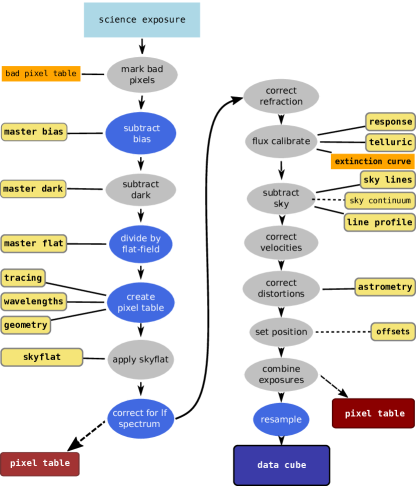
Figure 2: An idea for the scientific reduction algorithm for BlueMUSE.

As all ESO pipelines, the BlueMUSE pipeline will be embedded into the ESO data flow system, i.e., it will be implemented as part of CPL/HDRL plugins to the EsoRex[25] and EDPS[26] systems.

Based on the MUSE pipeline, we show a first flowchart for the science reduction of the BlueMUSE pipeline in Fig. 2. Since the instrument will be very similar, most of the steps will remain the same, from bad pixel masking using an external file, over bias subtraction, optional dark subtraction, and CCD-based flat-fielding using lamp-flat exposures. We then convert the images into tables of pixels using information on the location of the spectra (the tracing info), the wavelength calibration, and the instrument geometry. Onto these we apply the secondary sky-flat correction and correct the data for the overall shape of the lamp-flat spectrum, before correcting the data for atmospheric refraction. The refraction correction will likely work well using standard formulae and environmental measurements from the telescope telemetry in the FITS header.

The next step will apply the flux calibration using a response curve derived from a spectrophotometric standard, and apply an atmospheric extinction correction. This extinction correction could be derived from standard stars as well, if several were taken during photometric conditions in the same night at different airmasses. The flux calibration will include the possibility to correct telluric correction, even though no significant molecular absorption bands are expected to be visible in the wavelength range of BlueMUSE. The sky subtraction, distortion correction and astrometric position correction, as well as the exposure combination will work in the same way for BlueMUSE as they did for MUSE. The correction to (barycentric) velocity can be improved from recent work for other ESO pipelines (e.g., ESPRESSO), based on code from the SOFA[29, 30] / ERFA initiative.

While saving of the pixel tables is no longer necessary at any step, we foresee the option of saving the intermediate files after all, to let users optimize the data in different ways, even using code outside the pipeline proper. All steps of the science reduction of BlueMUSE will be executable as one integrated pipeline and as finegrained steps using the same library functions for testing and debugging.

As for MUSE, we will delay the sampling of the data into the regular grid of a datacube only as the very last step of the science reduction. But for BlueMUSE we will take into account the covariance (see Sect. 4.3) and also propagate the spectral line profile throughout of resampling.

4 BlueMUSE PIPELINE: SPECIFIC IMPROVEMENTS

We have so far studied at a few specific items that we will implement in a different way in the BlueMUSE pipeline. We will discuss three of them in this section.

4.1 Wavelength calibration

One of the main differences with regard to the MUSE instrument is that the wavelength calibration using arc lamps will not work as well in the blue wavelength range. The calibration unit (CU)[31] will therefore be using a Fabry-Perot system or a laser frequency comb as the light source to densely populate the spectral range. This will create a near-equal spaced lines on the detector, so that the association of lines to reference wavelengths will not work with the pattern matching implemented before[4]. Instead, we will create an initial zero-order calibration based on a standard arc-lamp exposure, and then construct the fully sampled wavelength solution using all lines from the comb or Fabry-Perot system. To save space, the full wavelength solution will be saved as a two-dimensional polynomial for each slice of the BlueMUSE instrument.

4.2 Line-spread function

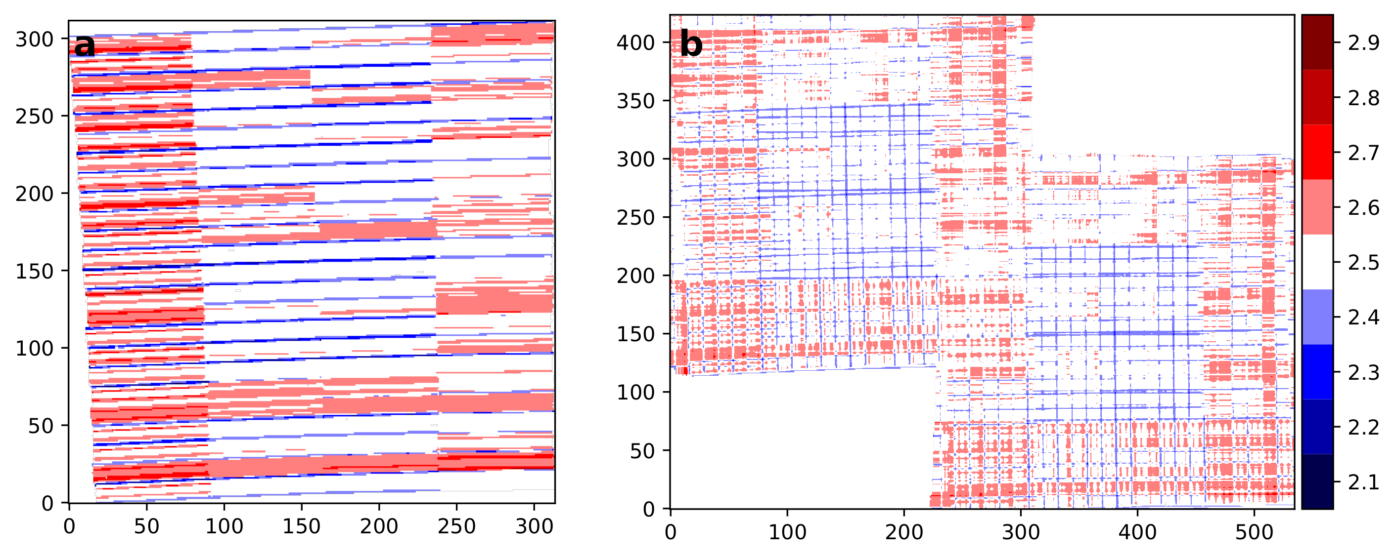
Figure 3: Spatially resolved line-spread function FWHM over the MUSE field. (a): LSF at 657.4 nm propagated to the cube of a single MUSE exposure. The FWHM varies between about 2.1 and 2.9 Å width. (b): LSF at the same wavelength, but for a MUSE cube created from six partially overlapping exposures, taken at 0, 90, and 180^∘ angles. The variations were smoothed out and range only between about 2.3 and 2.7 Å FWHM.

Using the Fabry-Perot setup of the BlueMUSE CU, we should be able to improve on the estimation of the line-spread function (LSF) that was based only on a few bright arc lines in the MUSE instrument. We are planning to use scanning techniques to sample the LSF at better resolution than single arc lines allow. We will therefore be able to derive the LSF not only for each slice of the instrument, but for even for spatial positions along the slices.

The LSF will be used within the pipeline to improve the sky subtraction. But to make it available to users of the instrument for the science analysis we will also propagate it through the data reduction and create a datacube of the instrumental profile (at least in terms of its FWHM). First tests doing that were conducted with the MUSE pipeline for existing data, the results are shown in Fig. 3. We can see that the pattern in a single exposure (Fig. 3a) clearly shows the pattern of the slices, which are the smallest elements for which we know the LSF. When combining more exposures that were taken with rotational and positional offsets, the differences are smoothed out (see Fig. 3b). In the analysis, LSF information like this can be further propagated through, e.g., Voronoi binning[32] to be used for stellar population fits with tools like pPXF[33].

4.3 Covariance propagation

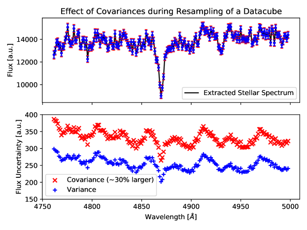
Figure 4: Stellar spectrum extracted from a partial MUSE observation with the estimated flux uncertainties, which were calculated with (red) and without (blue) taking the covariances into account. It is apparent that in this case the uncertainties are approximately 30% larger when taking covariances into account.

One part of the MUSE pipline is resampling the data from an irregular to a regular grid to create a datacube object[4]. This process causes variance values of single pixels to be transferred into covariances. The pipeline authors argue[4] that it would be infeasible to carry these covariances through further pipeline steps due to the size of the data involved. Since the MUSE pipeline only resamples the data once, the variances per voxel of the output datacube are still accurate. However, combining multiple voxels from a datacube in further analyses beyond the scope of the reduction pipeline without considering the involved covariances could cause significant underestimation of the uncertainties of flux values.

While it is true that the full covariance matrix would be too large to handle, it turns out that most entries of this matrix are zero. Each resampling method implemented in the MUSE pipeline only considers pixel values that are in some spatial and spectral proximity to the position of the output voxel. Therefore, covariances of a voxel are only offset from zero for other voxels in its proximity. With this in mind, the number of entries that are non-zero is likely small enough to be manageable for a whole datacube.

To put this to the test we implemented the drizzle-like resampling from the MUSE pipeline. We then added the handling of covariances according to the approach used for the pipeline of the Mapping Nearby Galaxies at Apache Point Observatory (MaNGA)[34]. We applied this algorithm to a spatially and spectrally limited part of a MUSE observation and extracted the spectrum of a single star from the reduced datacube. This spectrum is shown in the upper panel of Fig. 4. The flux uncertainties that are shown in that panel and the lower panel were calculated with and without taking the covariances into account. It is apparent that uncertainties derived only from variances are about 30% smaller than the ones derived by including the covariances.

The next step is to implement this method in the existing MUSE pipeline and run it on a full MUSE observation. While we expect that the additional computation time cost is not significant, this still needs to be tested. Based on the reduction with covariances described above, we anticipate that the additional storage size needed is in the order of $10\,$GB for a full MUSE observation using the drizzle-like resampling method. This estimate would change for other resampling methods that take into account pixels that are further away from the output voxel. Overall, this seems to be a promising approach to account for covariances during reduction with the MUSE pipeline.

5 BlueMUSE SIMULATIONS

In the late preparation phase before first light of MUSE, the consortium worked on a ’QSIM’ tool to produce synthetic data cubes reflecting targeted science observations. These were intended to allow the different science teams to prepare their individual analysis tools on data that would be as close to the final data products as feasible while being able to generate these mock data in a reasonable amount of time on their local desktop machines. An alternative tool, called the Instrument Numerical Model (INM)[35, 36], was able to simulate raw MUSE calibration and science exposures, but required computations of several days on a powerful workstation to generate the data. These in turn then had to be reduced using the data reduction pipeline to create datacubes. Compared to this, the QSIM datacube simulator was a very lightweight tool to generate datacubes quickly.

In 2013 QSIM was rewritten by M. Wendt from scratch in Python 2.X on the basis of the MUSE Python Data Analysis Framework (MPDAF) developed at the same time in Lyon [37]. In the end only few science simulations were realized before the First Light of MUSE itself. Namely, mockup cubes of parts of the UDF fields as well as a comprehensive simulation of a globular cluster field containing about 38,000 stars that also served as testing ground for resolving stellar populations with crowded field 3D spectroscopy[38]. Fortunately, the MUSE instrument was very successful right from the start and even the commissioning data led to science publications. In particular of the globular cluster NGC 6397, featuring the aforementioned crowded field spectroscopy[39] and a transverse science case directly motivated by the earlier simulations[40]. Once real instrument data was available, there was little use for a simulation tool in its state at the time.

5.1 Development of simulation software for BlueMUSE

During the preparation for the upcoming MUSE data before commissioning, it became obvious that the future end users of the final data products needed to get ready to deal with that kind of data in terms of sheer volume and also the limited ability of common tools to handle 3-dimensional data sets. In contrast, future users of BlueMUSE will be able to draw from a large pool of released tools and experience as well as laptop sized hardware that is easily up to the task of managing the expected data end products. A lesson learned from the development of dedicated simulation tools is that they need to be available way ahead of the planning of science observation since this is where simulations can play out their full potential. Accessing feasiblity and requirements for certain scientific questions in relation to a group of objects. While software like the provided exposure time calculator (ETC) will provide estimates of the expected signal-to-noise for a given observation, its impact on the success of the scientific exploitation of the data can only be tested and confirmed deploying the full analysis chain on the data. A number – but not all – of the questions that can and should be tackled ahead of the observation proposals are:

• What is the minimum S/N at which we can expect to detect the characteristic features of interest?

• Is the given resolution as well as the binsize appropriate for the set goals?

• How much is the data being affected by the (reduced) transmission of the instrument (at the lower wavelength end)?

• Are sky emission and telluric absorption lines a problem for the specific redshift range?

To successfully tackle those questions, the simulations need to create as realistic as possible data that mimics the expected data product from the offical data reduction pipeline closely. This includes the geometrical properties of the data cube and the plain instrumental parameters such as the spatial and spectral sampling, the spectral resolution as well as the overall cube dimensions as mentioned in section 1. Naturally it needs an interface to implement various science objects in the simulations, ranging from individual point sources such as quasars to clusters of stars, groups of galaxies or even diffuse emission.

But it also has to implement the simulated observing conditions, most notably the seeing conditions but also the full composition of the telluric background and the resulting complex noise properties of the data. The infamous ’redshift desert’ for example – the inability or lowered sensitivity to appropiately determine galaxy redshifts in a certain redshift range (usually $1.4<z<1.9$) – can in part be attributed to the lack of suitable emission lines in the optical for certain redshift ranges but a major aspect is the contamination with telluric features for higher wavelength ranges. Even single features can have influence on detection software, which is only one aspect why an accurate sky modelling is fundamental.

To address the mentioned points, a completely new software is currently being developed at Potsdam University to simulate BlueMUSE data: ’BlueSi’. Where the former QSIM relied on frequent changes of an early MPDAF development version and on Python 2.x the focus is now on user-friendlyness and long-term maintainability to have a ready-to-use product in Python 3.x already in the science planning phase of the instrument. In the current early state, the BlueMUSE simulation software ’BlueSi’ implements a Python interface to The Cerro Paranal Advanced Sky Model which allows the user to either manually vary up to 36 parameters related to physical conditions or simply mimic the conditions at a specific day and time and optionally merely provide deviations to those. This will allow the user to make very detailed choices while also being able to rely on realistic default settings.

The latter point turned out to be crucial in the usability and overall value of such simulations software and it also affects the inclusion of science objects into the simulated data cubes. While the simulation software for MUSE allowed for very complex and specific objects such as galaxies with separated information on different stellar populations with their own distributions and kinematics along with parametrized rotational curves and dispersion maps of any number of emission lines, it was basically impossible for a non-expert in all of those fields to generate realistic representations of typical galaxies. The mere preparation of the source file in the proper format constituted a significant obstacle.

To provide a much smoother learning curve and ease the process of simulating data products for a range of science cases, we work in close contact with the potential future users to help create an intuitive user interface and data format per major science case. We hope that by establishing a range of actual science objects as provided by the related peer-group the threshold to derive new science objects as targets for the BlueSi software will be significantly lowered.

As part of the current efforts, we implement a simulation of a globular cluster based on the data and analysis of MUSE observations. The detailed study of NGC 3201[41] allows us to to make use of a large data base of synthetic stellar spectra (PHOENIX[42]) based on the derived stellar parameters. These synthetic spectra cover the full wavelength range of BlueMUSE and are computed at very high resolution ($R\sim 500,000$). Naturally, the simulation also needs to incorporate the features related to the cluster itself, such as the individual radial velocities of the stars and their intrinsic magnitudes.

The different steps involved in defining the data format and interface to the simulation software will be documented and serve as a blueprint for further integration.

6 CONCLUSIONS AND OUTLOOK

Despite some issues, the MUSE integral field spectrograph and its pipeline are a major success. The pipeline was already in a good shape to support commissioning activities in 2014 and first science papers shortly thereafter. Most of the shortcomings of the pipeline are understood and will be rectified in the design of the BlueMUSE pipeline, with MUSE data and pipeline as its testbed.

Specific improvements planned for the BlueMUSE data reduction are a simpler structure with better parallelization, improved wavelength calibration through Fabry-Perot or frequency comb techniques, a more detailed knowledge of the line-spread function, and the propagation of covariance to the final datacube.

To support science studies, a new simulation suite ’BlueSi’ is being developed, with globular clusters as the first case to test generation of a realistic datacube.

The BlueMUSE integral field spectrograph is currently in its internal Phase A study phase and will enter the formal process with ESO in 2024. It is planned to be installed at the VLT in 2030 by which time its pipeline should be largely finished and ready for testing on sky.

- [1] Bacon, R., Accardo, M., Adjali, L., Anwand, H., Bauer, S., et al., “The MUSE second-generation VLT instrument,” in [Ground-based and Airborne Instrumentation for Astronomy III ], Proc. SPIE 7735 (July 2010).
- [2] Bacon, R., Vernet, J., Borisova, E., Bouché, N., Brinchmann, J., et al., “MUSE Commissioning,” The Messenger 157, 13–16 (Sept. 2014).
- [3] Richard, J., Bacon, R., Blaizot, J., Boissier, S., Boselli, A., et al., “BlueMUSE: Project Overview and Science Cases,” arXiv (Jun 2019). BlueMUSE white paper, arXiv:1906.01657.
- [4] Weilbacher, P. M., Palsa, R., Streicher, O., Bacon, R., Urrutia, T., et al., “The Data Processing Pipeline for the MUSE Instrument,” A&A 641, A28 (Sept. 2020).
- [5] Irwin, P. G. J., Toledo, D., Braude, A. S., Bacon, R., Weilbacher, P. M., et al., “Latitudinal variation in the abundance of methane (CH4) above the clouds in Neptune’s atmosphere from VLT/MUSE Narrow Field Mode Observations,” Icarus 331, 69–82 (Oct 2019).
- [6] Opitom, C., Yang, B., Selman, F., and Reyes, C., “First observations of an outbursting comet with the MUSE integral-field spectrograph,” A&A 628, A128 (Aug. 2019).
- [7] McLeod, A. F., Weilbacher, P. M., Ginsburg, A., Dale, J. E., Ramsay, S., and Testi, L., “A nebular analysis of the central Orion nebula with MUSE,” MNRAS 455, 4057–4086 (Feb. 2016).
- [8] Monreal-Ibero, A. and Walsh, J. R., “The MUSE view of the planetary nebula NGC 3132,” A&A 634, A47 (Feb. 2020).
- [9] Kamann, S., Husser, T. O., Dreizler, S., Emsellem, E., Weilbacher, P. M., et al., “A stellar census in globular clusters with MUSE: The contribution of rotation to cluster dynamics studied with 200 000 stars,” MNRAS 473, 5591–5616 (Feb 2018).
- [10] Giesers, B., Kamann, S., Dreizler, S., Husser, T.-O., Askar, A., et al., “A stellar census in globular clusters with MUSE: Binaries in NGC 3201,” A&A 632, A3 (Dec. 2019).
- [11] Roth, M. M., Sandin, C., Kamann, S., Husser, T.-O., Weilbacher, P. M., et al., “MUSE crowded field 3D spectroscopy in NGC 300. I. First results from central fields,” A&A 618, A3 (Oct. 2018).
- [12] Kollatschny, W., Weilbacher, P. M., Ochmann, M. W., Chelouche, D., Monreal-Ibero, A., et al., “NGC 6240: A triple nucleus system in the advanced or final state of merging,” A&A 633, A79 (Jan. 2020).
- [13] Emsellem, E., Schinnerer, E., Santoro, F., Belfiore, F., Pessa, I., et al., “The PHANGS-MUSE survey. Probing the chemo-dynamical evolution of disc galaxies,” A&A 659, A191 (Mar. 2022).
- [14] Wisotzki, L., Bacon, R., Brinchmann, J., Cantalupo, S., Richter, P., et al., “Nearly all the sky is covered by Lyman- emission around high-redshift galaxies,” Nature 562, 229–232 (Oct 2018).
- [15] Bacon, R., Mary, D., Garel, T., Blaizot, J., Maseda, M., et al., “The MUSE Extremely Deep Field: The cosmic web in emission at high redshift,” A&A 647, A107 (Mar. 2021).
- [16] Emsellem, E., Krajnovic, D., and Sarzi, M., “A kinematically distinct core and minor-axis rotation: the MUSE perspective on M87.,” MNRAS 445, L79–L83 (Nov. 2014).
- [17] Fumagalli, M., Fossati, M., Hau, G. K. T., Gavazzi, G., Bower, R., et al., “MUSE sneaks a peek at extreme ram-pressure stripping events - I. A kinematic study of the archetypal galaxy ESO137-001,” MNRAS 445, 4335–4344 (Dec. 2014).
- [18] Soto, K. T., Lilly, S. J., Bacon, R., Richard, J., and Conseil, S., “ZAP - enhanced PCA sky subtraction for integral field spectroscopy,” MNRAS 458, 3210–3220 (May 2016).
- [19] Cantalupo, S., Pezzulli, G., Lilly, S. J., Marino, R. A., Gallego, S. G., et al., “The large- and small-scale properties of the intergalactic gas in the Slug Ly nebula revealed by MUSE He II emission observations,” MNRAS 483, 5188–5204 (Mar. 2019).
- [20] Husemann, B., Singha, M., Scharwächter, J., McElroy, R., Neumann, J., et al., “The Close AGN Reference Survey (CARS). IFU survey data and the BH mass dependence of long-term AGN variability,” A&A 659, A124 (Mar. 2022).
- [21] Bacon, R., Brinchmann, J., Richard, J., Contini, T., Drake, A., et al., “The MUSE 3D view of the Hubble Deep Field South,” A&A 575, A75 (Mar. 2015).
- [22] Urrutia, T., Wisotzki, L., Kerutt, J., Schmidt, K. B., Herenz, E. C., et al., “The MUSE-Wide Survey: survey description and first data release,” A&A 624, A141 (Apr 2019).
- [23] Richard, J., Bacon, R., Vernet, J., Wylezalek, D., Valenti, E., et al., MUSE User Manual. ESO (Aug. 2019). ESO-261650, v10.4.
- [24] Bacon, R., Conseil, S., Mary, D., Brinchmann, J., Shepherd, M., et al., “The MUSE Hubble Ultra Deep Field Survey. I. Survey description, data reduction, and source detection,” A&A 608, A1 (Nov 2017).
- [25] ESO CPL Development Team, “EsoRex: ESO Recipe Execution Tool.” Astrophysics Source Code Library (Apr. 2015). ascl:1504.003.
- [26] Freudling, W., “The ESO Data Processing System (EDPS): A unified system for science data processing,” in [Proc. SPIE ], 12186, 1218612 (2022).
- [27] Smette, A., Sana, H., Noll, S., Horst, H., Kausch, W., et al., “Molecfit: A general tool for telluric absorption correction. I. Method and application to ESO instruments,” A&A 576, A77 (Apr. 2015).
- [28] Smette, A., Kausch, W., Sana, H., Noll, S., Horst, H., et al., “Molecfit: Telluric absorption correction tool.” Astrophysics Source Code Library (Jan. 2015).
- [29] Wallace, P. T., “The IAU SOFA Initiative,” in [Astronomical Data Analysis Software and Systems V ], Jacoby, G. H. and Barnes, J., eds., Astronomical Society of the Pacific Conference Series 101, 207 (Jan. 1996).
- [30] IAU SOFA Center, “SOFA: Standards of Fundamental Astronomy.” Astrophysics Source Code Library, record ascl:1403.026 (Mar. 2014).
- [31] Roth, M. M., Kelz, A., Madhav, K., Weilbacher, P. M., Richard, J., et al., “The BlueMUSE Calibration Unit: Phase-A studies,” in [Proc. SPIE ], 12184, 12184–217 (2022).
- [32] Cappellari, M. and Copin, Y., “Adaptive spatial binning of integral-field spectroscopic data using Voronoi tessellations,” MNRAS 342, 345–354 (June 2003).
- [33] Cappellari, M., “Improving the full spectrum fitting method: accurate convolution with Gauss-Hermite functions,” MNRAS 466, 798–811 (Apr. 2017).
- [34] Law, D. R., Cherinka, B., Yan, R., Andrews, B. H., Bershady, M. A., et al., “The Data Reduction Pipeline for the SDSS-IV MaNGA IFU Galaxy Survey,” AJ 152, 83 (Oct. 2016).
- [35] Jarno, A., Bacon, R., Ferruit, P., and Pécontal-Rousset, A., “Numerical Simulation of the VLT/MUSE Instrument,” in [Astronomical Data Analysis Software and Systems XVII ], Argyle, R. W., Bunclark, P. S., and Lewis, J. R., eds., ASP Conf. Ser. 394, 701 (Aug. 2008).
- [36] Jarno, A., Bacon, R., Ferruit, P., Pécontal-Rousset, A., Pandey-Pommier, M., et al., “Introducing atmospheric effects in the numerical simulation of the VLT/MUSE instrument,” in [Modeling, Systems Engineering, and Project Management for Astronomy IV ], Proc. SPIE 7738 (July 2010).
- [37] Bacon, R., Piqueras, L., Conseil, S., Richard, J., and Shepherd, M., “MPDAF: MUSE Python Data Analysis Framework.” Astrophysics Source Code Library (Nov 2016). ascl:1611.003.
- [38] Kamann, S., Wisotzki, L., and Roth, M. M., “Resolving stellar populations with crowded field 3D spectroscopy,” A&A 549, A71 (Jan. 2013).
- [39] Husser, T.-O., Kamann, S., Dreizler, S., Wendt, M., Wulff, N., et al., “MUSE crowded field 3D spectroscopy of over 12 000 stars in the globular cluster NGC 6397. I. The first comprehensive HRD of a globular cluster,” A&A 588, A148 (Apr. 2016).
- [40] Wendt, M., Husser, T.-O., Kamann, S., Monreal-Ibero, A., Richter, P., et al., “Mapping diffuse interstellar bands in the local ISM on small scales via MUSE 3D spectroscopy. A pilot study based on globular cluster NGC 6397,” A&A 607, A133 (Nov. 2017).
- [41] Giesers, B., Dreizler, S., Husser, T.-O., Kamann, S., Anglada Escudé, G., et al., “A detached stellar-mass black hole candidate in the globular cluster NGC 3201,” MNRAS 475, L15–L19 (Mar. 2018).
- [42] Husser, T. O., Wende-von Berg, S., Dreizler, S., Homeier, D., Reiners, A., et al., “A new extensive library of PHOENIX stellar atmospheres and synthetic spectra,” A&A 553, A6 (May 2013).