Color Dependence of the Transit Detectability for Young Active M-dwarfs

Abstract

We investigate the planetary transit detectability in the presence of stellar rotational activity from light curves for young M-dwarfs and estimate improvements of the detection at near-infrared (NIR) wavelengths. Making maps of the transit signal detection efficiency over the orbital period and planetary radius with light curves of members of four clusters, Hyades, Praesepe, Pleiades, and Upper Scorpius observed by the K2 mission, we evaluate the detectability for the rotation period and modulation semi-amplitude. We find that the detection efficiency remarkably decreases to about 20% for rapidly rotators with $P_{\rm rot}\leq 1$ d and the lack of planets in Pleiades is likely due to the high fraction of rapidly rotating M-dwarfs. We also evaluate the improvements of the planet detection with NIR photometry via tests using mock light curves assuming that the signal amplitude of stellar rotation decreases at NIR wavelengths. Our results suggest that NIR photometric monitoring would double relative detection efficiency for transiting planetary candidates with $P_{\rm rot}\leq 1$ d and find planets around M-dwarfs with approximately 100 Myr missing in the past transit surveys from the space.

1 Introduction

Although thousands of planets have been confirmed in the last few decades, the formation and evolution processes of planetary systems remain veiled in many aspects. Planetary evolution can be inferred in snapshots of young planetary systems in specific age stages. Recently, the secondary mission of the Kepler space telescope K2 (Borucki et al., 2010; Howell et al., 2014) and TESS (Ricker et al., 2015) reported young planets belonging to clusters (e.g., Mann et al., 2016a, b; Newton et al., 2019; Rizzuto et al., 2020), which have provided insights into the physics of the young systems. For example, radial inflation of young planets likely leads to atmospheric escape through stellar radiation (Owen, 2019). The number of detected planets in each cluster may also constrain the time-scale of their evolutionary stage.

Planetary systems around low luminosity M-dwarfs are targeted for biosignatures, because their habitable planet(s) might locate close to the host star, which is observationally preferable (Scalo et al., 2007; Kopparapu et al., 2013). Moreover, the observable planetary signals in both radial-velocity (RV) measurements and transit photometry are larger than those around solar-type stars, implying that M-dwarfs are ideal targets for finding small rocky planets and studying such planets’ atmospheres (e.g., Burke & McCullough, 2014).

Table 1: Young transiting planets confirmed in clusters or associations by the space missions.

Name	Host star temperature [K]	Planetary radius [$R_{\oplus}$]	Orbital period [d]	Reference
$Upper~{}Sco~{}~{}(\sim 10~{}{\rm Myr})$
K2-33 b ∗	$3540\pm 70$	$5.04_{-0.37}^{+0.34}$	$5.425\pm<0.001$	David et al. (2016); Mann et al. (2016b)∘
$Low~{}Cen~{}~{}(\sim 11~{}{\rm Myr})$
TOI-1227 b	$3072\pm 74$	$9.37_{-0.57}^{+0.74}$	$27.363\pm<0.001$	Mann et al. (2021)
$Sco{\rm-}Cen~{}~{}(\sim 17~{}{\rm Myr})$
HIP67522 b	$5675\pm 75$	$9.72_{-0.47}^{+0.48}$	$6.960\pm<0.001$	Rizzuto et al. (2020)
$Beta~{}Pictoris~{}Moving~{}Group~{}~{}(\sim 22~{}{\rm Myr})$
AU Mic b	$3700\pm 100$	$4.20\pm 0.20$	$8.463\pm<0.001$	Plavchan et al. (2020)
AU Mic c	$3700\pm 100$	$2.79_{-0.30}^{+0.31}$	$18.859\pm<0.001$	Martioli et al. (2021); Gilbert et al. (2022)∘
$Taurus{\rm-}Auriga~{}~{}(\sim 23~{}{\rm Myr})$
V1298 Tau b	$4970\pm 120$	$10.27_{-0.53}^{+0.58}$	$24.140\pm 0.002$	David et al. (2019)
V1298 Tau c	$4970\pm 120$	$5.59_{-0.32}^{+0.36}$	$8.250\pm<0.001$
V1298 Tau d	$4970\pm 120$	$6.41_{-0.40}^{+0.45}$	$12.403\pm 0.002$
V1298 Tau e	$4970\pm 120$	$8.74_{-0.72}^{+0.84}$	$60_{-18}^{+60}$
$IC~{}2602~{}~{}(\sim 35~{}{\rm Myr})$
TOI-837 b	$6407\pm 162$	$8.45\pm{0.99}$	$8.325\pm<0.001$	Bouma et al. (2020)
$Tuc{\rm-}Hor~{}~{}(\sim 40~{}{\rm Myr})$
DS Tuc A b	$5542\pm 21$	$5.63_{-0.21}^{+0.22}$	$8.139\pm 0.001$	Benatti et al. (2019)∘; Newton et al. (2019)
$Cep{\rm-}Her~{}~{}(\sim 40~{}{\rm Myr})$
Kepler-1627 A b	$5505\pm 60$	$3.78\pm{0.16}$	$7.203\pm<0.001$	Bouma et al. (2022a)
Kepler-1643 b	$4916\pm 110$	$2.32\pm{0.14}$	$5.323\pm<0.001$	Bouma et al. (2022b)
KOI-7368 b	$5241\pm 100$	$2.22\pm{0.12}$	$6.843\pm<0.001$	Bouma et al. (2022b)
KOI-7913 A b	$4324\pm 70$	$2.34\pm{0.18}$	$24.279\pm<0.001$	Bouma et al. (2022b)
$MELANGE-3~{}~{}(\sim 105~{}{\rm Myr})$
Kepler-1928 b	$5720\pm 60$	$1.96_{-0.04}^{+0.06}$	$19.578\pm<0.001$	Barber et al. (2022)
Kepler-970 b	$4290\pm 70$	$2.47_{-0.06}^{+0.11}$	$16.737\pm<0.001$	Barber et al. (2022)
$Psc-Eri~{}~{}(\sim 120~{}{\rm Myr})$
TOI-451 b	$5550\pm 56$	$1.91\pm{0.12}$	$1.859\pm<0.001$	Newton et al. (2021)
TOI-451 c	$5550\pm 56$	$3.1\pm{0.13}$	$9.193\pm<0.001$
TOI-451 d	$5550\pm 56$	$4.07\pm{0.15}$	$16.365\pm<0.001$

Continuation of Table 1
Name Host star temperature [K] Planetary radius [$R_{\oplus}$] Orbital period [d] Reference a co-moving star group   $(\sim 200~{}{\rm Myr})$ TOI-1807 b $4757_{-50}^{+51}$ $1.85\pm{0.04}$ $0.549\pm<0.001$ Hedges et al. (2021) TOI-2076 b $5187_{-53}^{+54}$ $3.28\pm{0.04}$ $10.356\pm<0.001$ Hedges et al. (2021) TOI-2076 c $5187_{-53}^{+54}$ $4.44\pm{0.05}$ … TOI-2076 d $5187_{-53}^{+54}$ $4.14\pm{0.07}$ … $Group-X~{}~{}(\sim 300~{}{\rm Myr})$ TOI-2048 b $5185\pm 60$ $2.05_{-0.19}^{+0.20}$ $13.790\pm 0.001$ Newton et al. (2022) $Ursa~{}Major~{}~{}(\sim 400~{}{\rm Myr})$ HD 63433 b $5640\pm 74$ $2.15\pm 0.10$ $7.108\pm<0.001$ Mann et al. (2020) HD 63433 c $5640\pm 74$ $2.67\pm 0.12$ $20.545\pm 0.001$ $Praesepe~{}~{}(\sim 700~{}{\rm Myr})$ K2-95 b ^∗ $3410\pm 65$ $3.7\pm 0.2$ $10.135\pm 0.001$ Obermeier et al. (2016); Mann et al. (2017)^∘ K2-100 b $6120\pm 90$ $3.5\pm 0.2$ $1.674\pm<0.001$ Mann et al. (2017) K2-101 b $4819\pm 45$ $2.0\pm 0.1$ $14.677\pm 0.001$ Mann et al. (2017) K2-102 b $4695\pm 50$ $1.3\pm 0.1$ $9.916\pm 0.001$ Mann et al. (2017) K2-104 b ^∗ $3660\pm 67$ $1.9_{-0.1}^{+0.2}$ $1.974\pm 0.001$ Mann et al. (2017) K2-264 b ^∗ $3580\pm 70$ $2.27_{-0.16}^{+0.20}$ $5.840\pm<0.001$ Rizzuto et al. (2018) K2-264 c $3580\pm 70$ $2.77_{-0.18}^{+0.20}$ $19.664\pm<0.001$ $Hyades~{}~{}(\sim 700~{}{\rm Myr})$ HD 283869 b $4655\pm 55$ $1.96\pm 0.13$ $106_{-25}^{+74}$ Vanderburg et al. (2018) K2-25 b ^∗ $3180\pm 60$ $3.31_{-0.25}^{+0.34}$ $3.485\pm<0.001$ Mann et al. (2016a) K2-136A b $4499\pm 50$ $0.99_{-0.04}^{+0.06}$ $7.975\pm 0.001$ Ciardi et al. (2018); Livingston et al. (2018); Mann et al. (2018)^∘ K2-136A c $4499\pm 50$ $2.91_{-0.10}^{+0.11}$ $17.307\pm<0.001$ K2-136A d $4499\pm 50$ $1.45_{-0.08}^{+0.11}$ $25.575\pm 0.002$ $NGC6811~{}~{}(\sim 900~{}{\rm Myr})$ Kepler-66 b $5962\pm 79$ $2.80\pm 0.16$ $17.816\pm<0.001$ Meibom et al. (2013) Kepler-67 b $5331\pm 63$ $2.94\pm 0.16$ $15.726\pm<0.001$ Meibom et al. (2013) $Ruprecht~{}147~{}~{}(\sim 3~{}{\rm Gyr})$ K2-231 b $5695\pm 50$ $2.5\pm 0.2$ $13.842\pm 0.001$ Curtis et al. (2018)

Note: The targets marked with asterisk are systems with effective temperature of 3000 K - 4000K and orbital period of $\leq$ 10 d. We cite the orbital parameters from the references marked with open circle when two or more papers exist for each system.

However, young stars usually have highly active regions on their surface (e.g., star spots, plage, and faculae) and high rotation velocities, which manifest as significant variations on the light curves of space missions (Rizzuto et al., 2017). This variation contaminates the light curve and obfuscates the planetary transit signals. Stellar rotational activities also appear as noise or false planetary signals (so-called “stellar jitter”) in RV measurements (Klein & Donati, 2020; Cale et al., 2021; Klein et al., 2022). Consequently, only approximately 30 transiting planetary systems, which are shown in Table 1, have been confirmed and/or validated around young stars in the clusters. For M-dwarfs, whose effective temperatures are 3000 - 4000 K, only 8 systems are confirmed.

In order to constrain the time scales of planetary formation and migration, one must estimate the true frequency of young planets. In fact, the distribution of the currently discovered planets appears to be biased with respect to stellar ages. For example, planets have been detected in the very young Upper Scorpius cluster ($\sim 8$ Myr) (e.g., Mann et al., 2016b) and in Hyades and Praesepe ($\sim 700$ Myr) (e.g., Mann et al., 2016a; Rizzuto et al., 2018), where evolution events are assumedly completing, but no planets have been found in Pleiades, whose age is intermediate between Upper Scorpius and Hyades ($\sim 125$ Myr). Additionally, no planetary systems are detected around M-dwarfs with the age of about 100 Myr for all targeted clusters as listed in Table 1. If the planetary systems both outside and inside of clusters share unique statistical properties, their age distribution should indicate the evolutionary process itself. However, whether this trend is caused by true planetary frequency or the detection efficiency of the transit signal is unclear, because the decline of the planet detection might be affected by stellar activity. The stellar rotation period varies in the early stage due to spin-up with contraction and constant angular momentum and spin-down with braking by the magnetic field (Godoy-Rivera et al., 2021).

In analyses of TESS photometry, Nardiello et al. (2021) suggested that the detection biases in clusters depend on the photometric precision. We hypothesize that the planetary transit detectability around young active stars in K2 is significantly prevented by photometric variations in the light curves. The detectability with the stellar activity was often discussed for each cluster in previous studies (e.g., Mann et al., 2018), but the systematic interpretation across the clusters is not enough to conclude whether current planet distribution is biased by stellar activity or not.

Tansit detection of young planets will be improved at NIR wavelengths, because the flux variation by stellar activity, which has hindered transit detection, is wavelength dependent. Especially for M-dwarfs, the photometric variation amplitudes are expected to be much lower at NIR wavelengths. Recent NIR photometric observations have gradually confirmed this wavelength dependence for some young stars (Frasca et al., 2009; Morris et al., 2018; Miyakawa et al., 2021). For example, Miyakawa et al. (2021) suggest the variation amplitude might decreases from 56% to 17% in $J$ - band compared to in $Kp$ - band. If future NIR observations with either space and/or ground-based telescopes are carried out, the planetary systems around young stars overlooked in previous space missions performed at visible wavelengths might be discovered.

In this study, we evaluate the planetary detection efficiencies around M-dwarfs with respect to stellar rotation to understand the causes of the current planet distribution in stellar clusters. We perform calculations of the signal detection efficiency (SDE) over the orbital period and signal amplitude through the detection tests with the K2 light curves and discuss the systematic detectability across four clusters: Hyades, Praesepe, Pleiades, and Upper Scorpius. Furthermore, transit detection efficiencies are derived as a benchmark for the statistical assessment of young planets. We also estimate the extent to which observations at the NIR wavelengths improves the detectability and assess the benefit of these improvements for future observational missions.

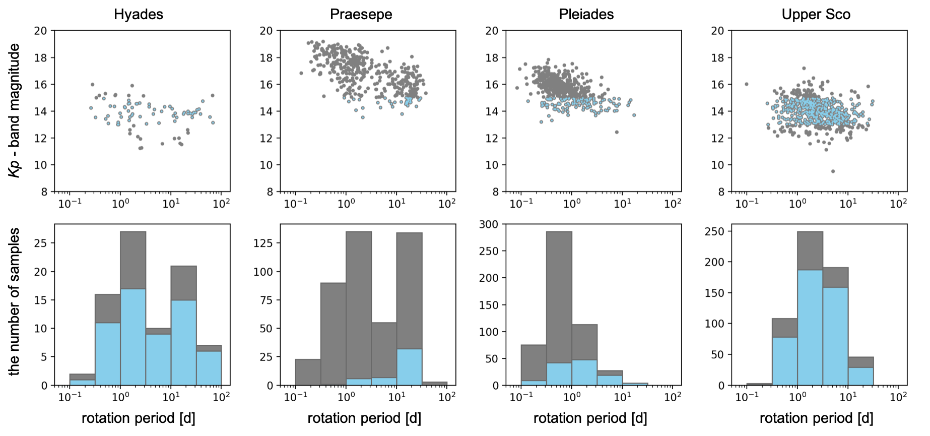
Figure 1: Top panels: scatter plots of the rotation period vs. apparent Kp magnitude for stars with 3000 K - 4000 K in four clusters. Bottom panels: histograms of the rotation periods in the clusters. The gray and blue data indicate the original members from the literatures and selected targets in this study, respectively.

The remainder of this paper is organized as follows. Section 2 introduces our targets and their selection process. Section 3 details the SDE mapping through the detection tests of transiting planets around active stars and Section 4 shows the test results over the clusters. Moreover, Section 5 shows improvement of the detection efficiency in the NIR through the test with mock light curves. Section 6 discusses biased frequencies of planets around active stars based on current observational results. A summary is given in Section 7.

2 Target Selection

This study focuses on planetary systems around young rapidly rotating M-dwarfs. The statistical properties of stars belonging to a given cluster are well determined. From the young stars in stellar clusters observed in the K2 mission, we selected targets whose rotation periods were determined in previous researches. Our original target lists and rotation periods in Pleiades, Praesepe, Upper Scorpius, and Hyades were taken from Rebull et al. (2016), Douglas et al. (2017), Rebull et al. (2018), and Douglas et al. (2019).

After matching the EPIC ID and 2MASS names of these targets, we downloaded their parallax and color information from the $Gaia$ EDR3 archive website (Gaia Collaboration et al., 2016, 2020; Collaboration, 2020). Because we focus on M-dwarfs, the targets were filtered through the range 3000 - 4000 K based on samples treated in Mann et al. (2015). The effective temperatures $T_{\rm eff}$ of each target was determined using the empirical $B_{P}-R_{P}$ vs. $T_{\rm eff}$ relation described in Mann et al. (2015). The apparent magnitudes in the Kp- band of the Kepler may also directly affect the detection result. Nardiello et al. (2021) showed that the detection efficiency of samples analyzed in the PATHOS (Nardiello, 2020; Nardiello et al., 2021) from the TESS targets. improves for brighter targets in the range of 6 - 18 ${\rm mag}_{T}$. To avoid this systematic bias, we filtered the targets through the magnitude range of $Kp$ = 13 - 15, sufficiently narrow to omit the trend while allowing a balanced representative of the samples in each cluster. After filtering, we obtained 61, 61, 121, and 476 light curves in Hyades, Praesepe, Pleiades, and Upper Scorpius, respectively.

The distributions for the stellar rotation period are shown in Figure 1. Upper panels show scatter plots of the rotation period vs. apparent magnitudes and lower panels show histograms for the rotation period for each cluster. The gray and blue data are original samples in the literature and selected samples in this study, respectively. For reference, the medians of the rotation periods from the literature are $2.45_{-1.69}^{+22.19}$ d, $2.06_{-1.47}^{+16.49}$ d, $0.63_{-0.33}^{+1.19}$ d, and $2.32_{-1.52}^{+5.09}$ d for Hyades, Praesepe, Pleiades, and Upper Scorpius, respectively. The uncertainties are estimated as range of 86th - 50th and 50th -14th percentile of the distribution. For Hyades and Upper Scorpius, we select samples at similar rates from the rotation-period bins. For Praesepe and Pleiades, relatively slow rotators are selected from the total samples. Note that we do not filter based on quality flags of the rotation period in the literature, thus periods larger than 30 d can be mis-detections or double of actual rotation periods.

3 Method

We perform the injection-recovery test of transiting planets for the clusters to evaluate the detection biases due to stellar activity (i.e., rotation period and flux variation). Firstly, we use light curves observed in K2 mission and investigate the biases to constrain true planet frequency for the current survey in Section 3 and 4. Moreover, we propose improvements in the planet detection in the NIR assuming future planet research in Section 5.

3.1 Light Curves

We use the light curves extracted by the pipeline of Vanderburg & Johnson (K2SFF; 2014), which are corrected with the centroid position of point-spread function. The correction is simply performed by fitting a polynomial function with respect to the spacecraft motion. The K2SFF light curves of our targets were downloaded from the Miltsuki Archive for Space Telescope portal website. Note that, we avoid using light curves extracted with machine learning - based pipelines, because miscorrection may be caused by high-cadence photometric variation and/or the existence of contamination of nearby stars in the clusters regions (Luger et al., 2016).

3.2 Injection of Planetary Transit Signals

To evaluate the detection efficiency of planetary transits, we injected mock signals into the $K2$ light curves over a wide range of orbital parameters. To remove the long-term trends from the light curves, we first binned the data points into five median bins and subtracted them from the original light curves by spline interpolation. In the light curves with discontinuous points caused by the spacecraft motion, the points before and after the missing points were corrected independently such that the light curves were smoothly connected. To ensure that the detectability of stellar rotational activities was unaffected by anomalies such as flares, the positive and negative outliers larger than $4-\sigma$ were replaced by unity. The robust standard deviation $\sigma$ was derived as 1.48 times the MAD in the robust statistics.

Next, we injected the planetary transit signal with the model of Ohta et al. (2009) for a given radius ratio $R_{\rm p}/R_{\rm s}$ and orbital period $P_{\rm orb}$. The limb-darkening of the host star was modeled with the quadratic functions in Claret & Bloemen (2011). To constrain the orbital parameters, the radius and mass were derived using the relations in $K$ band $M_{K}$ in Mann et al. (2015) and Mann et al. (2019), respectively. These relations use the absolute magnitude $M_{K}$ in the $K$ band, which is calculated from the parallaxes in $Gaia$ EDR3 and the $K$ band magnitudes in the 2MASS catalog (Skrutskie et al., 2003). We discuss uncertainties in the estimations of radius and effective temperature in Appendix A. To simplify the discussion, we set the eccentricity and impact parameter to 0.

To investigate the detectability in the orbital parameter space for each star, we calculated the signal detection efficiency (SDE) over the parameter space. We reproduced 100 transit signals on 10 $\times$ 10 grids of $R_{\rm p}/R_{\rm s}$ versus $P_{\rm orb}$ for each target considering the computational cost. The $R_{\rm p}/R_{\rm s}$ and $P_{\rm orb}$ scales were linearly spaced in [0.01, 0.2] and log-linearly spaced in [1 d, 30 d], respectively. The validity of the 10 $\times$ 10 simulations is discussed in Appendix C compared with 30 $\times$ 30 simulations.

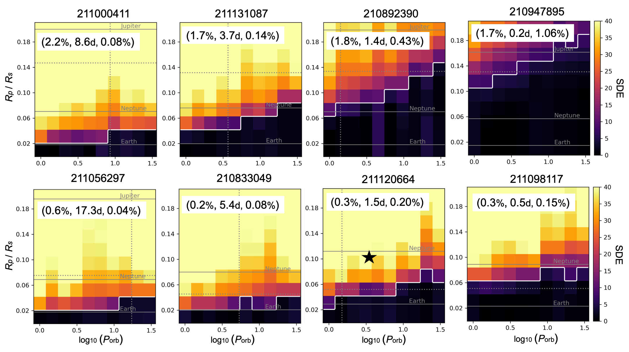
Figure 2: Examples of heat maps of the transit signal detection efficiency (SDE) for the 8 targets. The colors corresponds to the SDE in the transit least square (TLS; Hippke & Heller, 2019a) test with respect to the log-scale orbital period $P_{\rm orb}$ and relative planetary radius $R_{\rm p}/R_{\rm s}$ of the injected planet. The horizontal lines are converted planet radii of Earth, Neptune, or Jupiter, included as guides. The vertical and horizontal dotted lines represent the rotational period and the square root of the flux variation semi-amplitude, respectively. The white line is the boundary of SDE = 7 (the detection threshold). The photometric variation semi-amplitude, rotation period, and mean of the standard deviation in 0.3 d - sized bins of the detrended light curves ($A$, $P_{\rm rot}$, $\sigma_{\rm 0.3d}$) of the targets are shown in the top of the figures. The black star on the EPIC 211120664 is a projection of K2-25 b whose host star is the fastest rotator in confirmed planetary systems and shows similar light curve modulation to EPIC 211120664.

3.3 Evaluation of the SDE

We calculate the SDE of the injected planetary signals to evaluate the parameter regions where planets are detectable for each star. The normalization of the light curves were performed following the procedure in Mann et al. (2016a). We first computed the Lomb - Scargle (LS) periodogram (Scargle, 1982) to detect the significant variations which are possibly due to stellar rotational activity. We removed these signals in frequency space using the fast Fourier transform (FFT) and derived filtered light curves by inverting the spectral data to time space. The period search was performed in the range between one and 70 days to retain the planetary transit signals. The systematic trend were then removed thorough a median filter with a one-day window, and positive excursions larger than 3 - $\sigma$ with $1.48\times$ MAD were replaced by the median value.

Finally, the transit signals were recovered by the transit-least squares (TLS; Hippke & Heller, 2019a, b) algorithm, which is likely a more effective and reliable method to detect small transit signals than a previously popular box-fitting least square algorithm (Kovács et al., 2002). Besides, the TLS is optimal for V-shape light curves such as close-in planets around small host stars. Here we employed the TLS package implemented in Python code . As the input parameters of the TLS algorithm, we applied the stellar mass and radius derived by the relations with respect to $M_{K}$ in Mann et al. (2015) and Mann et al. (2019), respectively. The SDE value is calculated through the TLS for each period-radius segment of the 10 $\times$ 10 parameter space. To judge the recovery of the planetary signals, we set a threshold with the SDE of 7 based on the past works in the literature. Empirical thresholds are set between 6 and 10 (e.g., Dressing & Charbonneau, 2015; Wells et al., 2018).

Figure 3: Scatter plots colored by cluster. Panels (a), (b), and (c) plot the recovery rate $p$, the relative number of recovered tests to all tests using the 10 $\times$ 10 planetary parameters, vs. effective temperature, rotation period, and semi-amplitude of the photometric variation of the host stars, respectively. (d) plots the semi-amplitude of the variation vs. the rotation period.

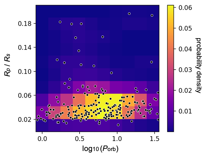
Figure 4: Probability density function (PDF) for planets around stars whose $T_{\rm eff}$ are 3000 - 4000 K discovered by the transit method. The black dots are orbital property of the planets. The probability density is calculated by the Gaussian kernel density estimation.

Figure 5: Scatter plots of $p_{\rm eff}$, effective recovery rate based on the current planet distribution, colored by cluster. The upper and lower panels are the detectability assuming the PDF in Figure 4 to the rotation period and semi-amplitude of the flux modulation, respectively.

4 Results

4.1 SDE Maps of Typical Targets

Through the injection and recovery tests described in Section 3, we visualized the detectability of the planetary signals as SDE maps of the $10\times 10$ orbital parameters in Figure 2. The vertical and horizontal dotted lines represent the rotation period and the square root of the flux variation semi-amplitude, respectively; the color bar corresponds to the SDE in the TLS test of each mock light curve; the white lines are the boundary of SDE = 7 as the detection threshold. The targets in the upper and lower rows show large and small amplitude variations, respectively. The rotation periods of the leftmost, center left, center right, and rightmost panels were approximately 10, 3, 1, and 0.3 days, respectively. In the top of each panel, we put the photometric variation amplitude $A$, rotation period $P_{\rm rot}$, and mean of the standard deviation in 0.3 d - sized bins $\sigma_{\rm 0.3d}$ as a rough standard of the photometric precision.

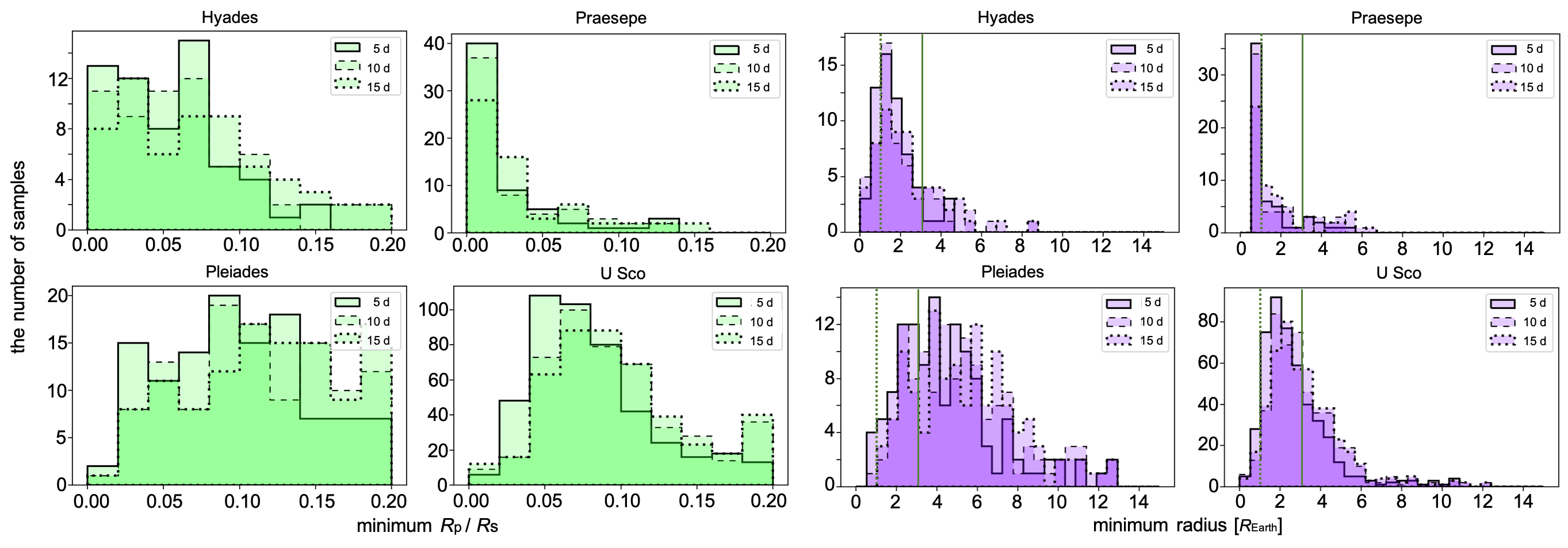
Figure 6: Histograms showing the number distributions of minimum detectable radius ratio $R_{\rm p}/R_{\rm s}$ (left) and planetary radius $R_{\rm p}[R_{\oplus}]$ (right) with SDE = 7 for a given orbital period in each cluster. In the right panels, dotted and dashed vertical lines denote the Earth and Neptune radii, respectively. The solid, dashed, and dotted lines denote different orbital periods of the injected planets (5, 10, and 15 d, respectively).

As shown in the upper panels, the detectability of the planetary candidates decreases with increasing rotational velocity. For the slowest rotator (EPIC 211000411), a radius ratio $R_{\rm p}/R_{\rm s}$ of 0.02, corresponding to a transit depth of $0.04\%$, is detectable. In this case, the detectability appears to be dominated by photometric precision, whose influence is discussed in Nardiello et al. (2021), rather than by stellar activity. In contrast, a planet around the rapid rotator with $P_{\rm rot}$ of $\leq$ 1 d (EPIC 210947895) is difficult to detect even at $R_{\rm p}/R_{\rm s}$ of 0.1 (= $1\%$ transit depth). In the lower panels, the detection limit for rapid rotators lies around $R_{\rm p}/R_{\rm s}$ = 0.05 ($\approx 0.3\%$ transit depth). These boundaries vary corresponding to the amplitudes of variations caused by stellar activity compared to the upper panels.

As a benchmark (black star in Figure 2), we selected a known planetary system orbiting a M-dwarf, K2-25b (EPIC 210490365b; Mann et al., 2016a), whose host star property is similar to EPIC 211120664. The relative planetary radius, orbital period, stellar rotation period, and amplitude of variation of the K2-25 system are approximately 0.1, 3.5 d, 1.9 d, and $1\%$, respectively. Although K2-25b orbits a very rapidly rotating M-dwarf, its rotational period and semi-amplitude of the variation are set significantly above the detection limit. Our results also indicate that if other Earth-sized planets exist around K2-25, they will be obscured by stellar activity.

Stellar activity appears to affect the detectability of planetary candidates especially when the stellar rotation periods are shorter than approximately three days. Pleiades and Upper Scorpius include a large number of such rapidly rotating stars (Rebull et al., 2016, 2018). In Hyades and Praesepe, there are large scatters of rotation periods in low-mass regions, and some targets (possibly binaries) rotate with periods shorter than three days (Douglas et al., 2019). Even when the variation amplitudes of the host stars are small (lower row of Figure 2), Earth-sized planets tend to be missed around the rapidly rotators with $P_{\rm rot}\leq 1$ d. TRAPPIST-1f, a habitable Earth-sized planet with a relative radius $R_{\rm p}/R_{\rm s}$ and orbital period of approximately 0.08 and 9 days, respectively, would not be detected in the TLS analysis, if the planet exists around active stars like EPIC 210892390, EPIC 210947895, and EPIC 211098117. Nonetheless, we are aware of sophisticated methods or optimizations (e.g., Rizzuto et al., 2017) that enhance the detectability of small planets around active stars.

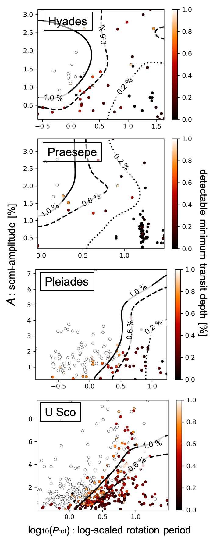
Figure 7: Scatter plot of the rotation period versus semi-amplitude of photometric variation for each cluster. The color bar corresponds to the minimum detectable transit depth [$(R_{\rm p}/R_{\rm s})^{2}\%$] when the orbital period is 10 d. The contour lines represent borders of 1.0%, 0.6%, and 0.2% detectable minimum transit depth. e.g., The targets existing above the border of 1.0% could not be detected when the transit depth is shallower than 1.0%.

4.2 Trends in the Simulations for the Whole Sample

We show the qualitative dependence of the test results on rotation period, and amplitude of the flux modulation to confirm correlations among the clusters. We calculate the proportion of recovered cases $p$ as a guide for interpretations. Here, $p$ defines the relative number of recovered tests to all tests using the 10 $\times$ 10 planetary parameters for each sample; $p=0$ and $p=1$ indicate that no planet is recovered and that all planets are recovered, respectively. of Figure 3-(a) displays the recovery-rate distribution for each cluster with respect to the effective temperature of the host star. The $T_{\rm eff}$ biases are likely introduced by distances to the cluster, because the samples were selected based on their apparent magnitudes. The samples in Pleiades and Upper Scorpius are more scattered along both the effective temperature and $p$ axes than those in Hyades and Praesepe. This difference may be caused by the different number of samples in each cluster. Despite these selection biases, the $p$ and the $T_{\rm eff}$ are apparently uncorrelated.

Figure 3-(b) and (c) display $p$ with respect to the rotation period $P_{\rm rot}$ and the semi-amplitudes of the light curve $A$, respectively. Unlike $T_{\rm eff}$, both $P_{\rm rot}$ and $A$ appear to influence the detectability $p$ with similar trends for each cluster. As shown in the scatter plot of $P_{\rm rot}$ versus $A$ (Figure 3 (d)), these two parameters are not clearly correlated despite their biased distributions in each cluster. Therefore, the trends displayed in panels (b) and (c) are independent. As a reference, the correlation coefficients are 0.49, -0.33, and -0.03 for panels (b), (c), and (d), respectively. Finally, we conclude that the detectability of the transit signals depends on the rotation period and amplitude of the flux modulation, respectively, rather than the effective temperature or cluster where the stars belong. Note that we do not discuss the detectability assuming a realistic exoplanet distribution, but a statistical trend in our simulation here.

4.3 Detectability Assuming the Observed Planetary Distribution

In this subsection, we derive an effective recovery rate $p_{\rm eff}$, a proportion of detectable planets when one transiting planet exists around each sample based on the current planet distribution. We downloaded a list of the orbital parameters of confirmed planets which were detected by the transit method around stars with $T_{\rm eff}$ of 3000 - 4000 K from NASA Exoplanet Archive (2019) . After removing the young planets listed in Table 1 from the list, we calculated a probability density function (PDF) for 249 confirmed planets by the Gaussian kernel density estimation which is shown in Figure 4. We derive the $p_{\rm eff}$ based on the observed planet distribution by multiplying the PDF by the detectability of the stellar activity for each pixel as $\delta_{\rm SDE}=\{\rm 1~{}(SDE\geq 7),~{}0~{}(SDE<7)\}$ and integrating over the orbital parameter region. Because the PDF is likely affected by the photometric precision, we avoid using a region where the radius ratio is less than 0.02 for this calculation.

We show the derived effective recovery rate $p_{\rm eff}$ to the rotation period and semi-amplitude of the flux modulation in the upper and lower panels of Figure 5, respectively. Compared with Figure 3 (b) and (c), samples seem to be biased toward the region where the $p_{\rm eff}$ is less than 0.4. This declination of $p_{\rm eff}$ is due to that the planetary distribution is dense around $R_{\rm p}/R_{\rm s}=$ 0.02 - 0.06 and $P_{\rm rot}=$ 5 - 10 d. The medians and ranges of 68 % distribution between stars of $p_{\rm eff}$ value are about $0.33_{-0.25}^{+0.58}$, $0.99_{-0.72}^{+0.01}$, $0.08_{-0.05}^{+0.42}$, and $0.16_{-0.11}^{+0.29}$ for Hyades, Praesepe, Pleiades, and Upper Scorpius, respectively. Note that these calculations are performed on assumption that the young planetary distribution is the same as the older counterpart.

4.4 Systematics of Each Cluster

Section 4.2 presented the statistical properties of the whole filtered samples. We now focus on the results for each cluster. Figure 6 shows histograms of the numbers of samples with respect to the minimum detectable radius ratio and converted radius.

Although the detectability decreases with increasing orbital period, the degradation is slight. For most of the samples in Hyades, Praesepe, and Upper Scorpius, the minimum $R_{\rm p}/R_{\rm s}$ detectable is less than 0.10 (left panels of Figure 6). The high detectability in Praesepe is attributable to the selection bias. As shown in Figure 1, we selected relatively bright targets and stars with high effective temperatures, for which the signal modulations are stable (Rebull et al., 2018). Although a similar selection bias exists in Pleiades targets, the distribution of detection limits in Pleiades is widely scattered, indicating that most of the Pleiades samples are more active than those of Praesepe.

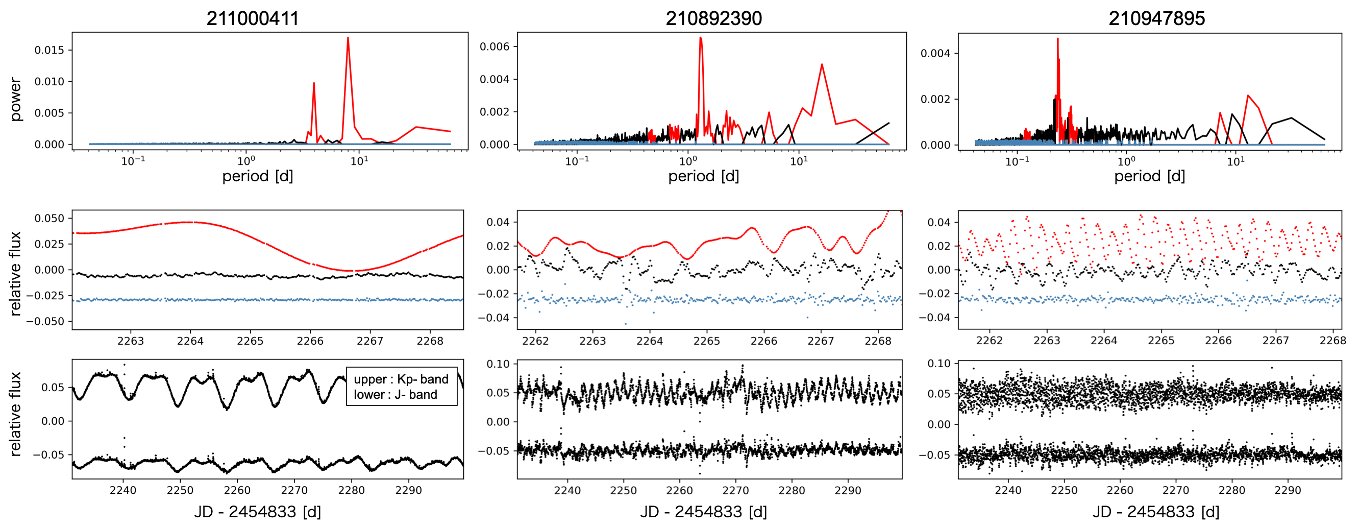
Figure 8: Explanations of the analysis in subsection 5.1 for three typical targets. For each target, the top panel plot the periodogram derived by FFT. The red, blue, and black data represent sinusoidal modulation detected by LS, white noise, and other correlated noise, respectively. In the middle panel, the range is narrowed to approximately five days to clarify the details of light curves reproduced by inverse FFT. The color relation is same to the top panel. The bottom panels plot the original light curves in the $Kp$-band (upper) and reproduced light curves assuming the $J$-band observation (lower).

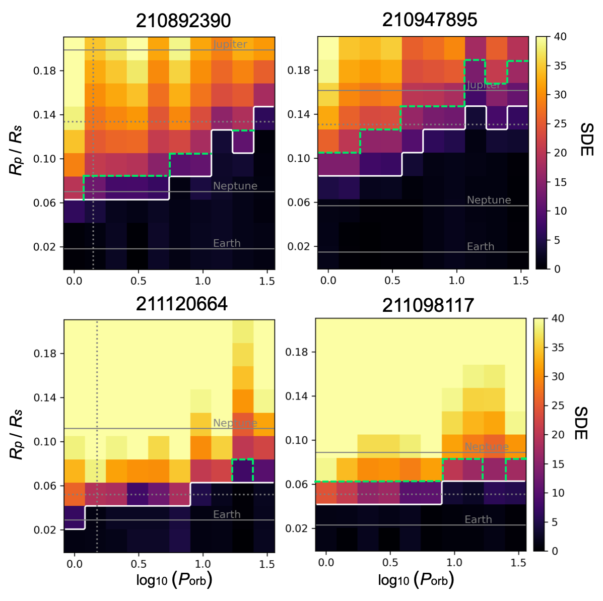
Figure 9: Same heat maps with the right side of Figure 2, but in the $J$- band. The dashed green lines represent the border in the $Kp$- band of Figure 2 for comparison.

To assist the astrophysical interpretation, we present the same histograms against the planetary radius in the right panels of Figure 6. For the histograms with the orbital period of 10 d, we derived the median planet radius and the fraction of stars for which Earth-size and Neptune-size planets can be detected ($f_{\rm Earth}$, $f_{\rm Neptune}$) for each cluster in Table LABEL:tab:res_hist. Neptune-sized planets are detected around most targets in Hyades and Praesepe, and a reasonable rate of samples passed the threshold of Earth-sized planets. In Upper Scorpius samples, most injected planets larger than Neptune were also detected. Conversely, planet detection among the Pleiades members was difficult and very few Earth-sized planets are detectable. Even for Neptune-sized planets, the passed fraction is only 20 %. Note that we may possibly underestimate the planetary distribution due to the inflation of stellar radius in the early stage and the detection in Pleiades and Upper Scorpius may be more difficult than we estimated.

In addition, we derived p-values by performing the Kolmogorov-Smirnov test for the histograms with the orbital period of 10 d to the Hyades, Praesepe, and Pleiades ($\rm P_{KS,Hya}$, $\rm P_{KS,Pra}$, and $\rm P_{KS,Ple}$) and listed them in Table LABEL:tab:res_hist. The distributions are different each other according to the small P-values ($<0.05$).

Figure 7 clarifies the relation between the detectability and light curve modulation. In this figure, the white circles represent the targets whose transit depths of less than 1% cannot be detected if planets exist around them. The detection limits have a trend from the left bottom to the right top in the plots of all clusters. We also show the contours which represent borders of 1.0 %, 0.6 %, and 0.2 % of the minimum detectable transit depths. The contours were estimated with Gaussian filtering with 1 $\sigma$ of 5 pix after the nearest 2D interpolation of the parameter space with 50 $\times$ 50 grids for the scattered data points. This systematic behavior can explain the distributions of detectable $R_{\rm p}/R_{\rm s}$ for each cluster in Figure 6, indicating that the detectability in Pleiades simply depends on the light curve feature. In general, cool stars rotate more rapidly than hot stars in their young phase. We selected relatively bright Pleiades members (see Figure 1), and other Pleiades members may be cooler and more rapid rotators than our targets. Thus, it will be more difficult to detect planetary transit signals for all the Pleiades members than we estimate in this study. Consistently with this assumption, no secure detection of transiting planets has been reported for Pleiades members (Gaidos et al., 2017).

5 Expectation in NIR Observations

Figure 10: Scatter plots of the semi-amplitude of photometric variation and detectable depth versus rotation period. The color bar presents the minimum detectable transit depth in the $Kp$- band. The red points are the detectable targets at a threshold of $1\%$ in the $J$- band, but not in the $Kp$- band. In the left, middle, and right panels, the planetary orbital periods of samples are 5, 10, and 15 days, respectively.

Table 2: Statistical values for the histogram in the right of Figure 6.

	Hyades	Praesepe	Pleiades	U Sco
${\rm P_{KS,Hya}}$	-	$4.9\times 10^{-5}$	$3.0\times 10^{-15}$	$3.7\times 10^{-8}$
${\rm P_{KS,Pra}}$	-	-	$4.4\times 10^{-16}$	$3.0\times 10^{-17}$
${\rm P_{KS,Ple}}$	-	-	-	$2.1\times 10^{-15}$
median [$R_{\oplus}$]	1.6	0.9	4.9	2.8
$f_{\rm Earth}$	0.20	0.60	0.01	0.04
$f_{\rm Neptune}$	0.80	0.84	0.20	0.56

5.1 Reproduction of the NIR Photometry

As mentioned in Section 1, the light curve variations caused by stellar activity are wavelength dependent. Some studies suggested a trend that the amplitude of the sinusoidal flux modulation is lower at NIR than at visual wavelengths by about 50 - 80 % for M-dwarfs (e.g., Frasca et al., 2009; Morris et al., 2018; Miyakawa et al., 2021). If this is the case for most active low-mass stars, then planetary detection around young targets should be enhanced in future transit search with NIR instruments. When evaluating the wavelength dependency of the detected transit signals and the efficiency of the NIR survey, we performed the test assuming observations in the NIR.

We first applied the FFT to the light curves observed with the $Kp$ - band in the K2 mission. To detect the frequencies of the sinusoidal modulation (i.e., stellar jitter), we also computed the LS periodogram. The amplitudes of the modulations corresponding to significant peaks in the LS periodogram (within $10\%$ uncertainty of the peaks detected in the LS and with false alarm probabilities below $1\%$) were adjusted to the $J$ - band observations. Here, the amplitude ratio of the $J$ to $Kp$ - bands, was assumed as $34.8\%$, the observational values derived as the mean of the four active M-dwarfs belonging to the Hyades in Miyakawa et al. (2021).

The white noise was determined as signals with powers lower than $F_{\rm med}+3\sigma$ in the FFT spectrum, where $F_{\rm med}$ and $\sigma$ are the median and standard deviation, respectively of the signals with frequencies exceeding $15~{}{\rm d}^{-1}$. In the $J$ - band, we re-scaled the white-noise scatter in the $Kp$ - band photometry based on the photon counts derived from the spectral energy distribution (SED), applying the PHOENIX spectra of Allard et al. (2013) as the SED model. The photometric flux for a given effective temperature of the host star was calculated as described in Fukugita et al. (1995). Note that we assume the same telescope profile with the Kepler because we focus on the wavelength dependency of the signal. After reproducing the NIR light curves through the above procedures, we applied the tests described in subsection 3.2 and 3.3.

Figure 8 demonstrates the analysis on three typical targets; EPIC 21100411, EPIC 210892390, and EPIC 210947895 with rotational periods of $\sim 10$ d, $\sim 1$ d, and $\sim 0.3$ d, respectively. In the FFT results of each target (upper panels), the red, blue, and black peaks were detected as astrophysical signals in the LS periodogram, white noise, and other correlated noise, respectively and the middle panels displays the corresponding light curves at the frequencies discriminated in the FFT of each target. The correlated noise for the rapid rotators (EPIC 210892390 and EPIC 210947895) is significantly larger than that of EPIC 21100411, possibly because the correlated noise is not easily distinguished from rotational modulation in the periodogram analysis. Consequently, the rotational modulations were underestimated, but this uncertainty did not affect our estimations of the lower limits of improvement in the mock $J$ - band observation. The multi-periodicities in EPIC 210892390 and EPIC 210947895 might be explained by differential rotation and/or binarity. In either case, the wavelength dependency of the rotational modulation will probably not vary significantly from the basic assumption. The bottom panels of Figure 8 show the original light curves and the mock light curves assuming $J$-band observations.

5.2 Improvement in NIR

The SDE maps of the rapid rotators EPIC 210892390, EPIC 210947895, EPIC 211120664, and EPIC 211098117 shown in Figure 2 are replotted assuming NIR observations in Figure 9. Also plotted in Figure 9 are the borders in $Kp$- band. Although the detectability was not apparently improved around slowly rotating ($P_{\rm rot}\sim 10$) - and less active ($A\sim 0.1\%$) -stars, the detectable relative radius $R_{\rm p}/R_{\rm s}$ was improved by at most 0.04 (corresponding to two grid widths) for the very active targets.

Figure 10 plots the semi-amplitude of the photometric variation and minimum detectable transit depth as functions of stellar rotation period for all targets derived in the injection and recovery tests. The left, middle, and right panels correspond to planetary orbital periods of 5, 10, and 15 days, respectively. Some targets (highlighted in red) were detectable at a threshold of $1\%$ in the $J$- band but not in the $Kp$- band. The limits in both $Kp$ and $J$- bands deteriorate with increasing orbital period, because the number of transit signals decreases in a given observation span. Targets that were detectable only in the $J$-band (red points) appear to be distributed in the upper left of those that were detectable in the $Kp$ band (gray - black points), regardless of orbital periods. Such targets are likely members of Pleiades and Upper Scorpius, where active targets dominate (see Figure 3-(d)).

To evaluate the detectability, we plot the accumulated distribution in Figure 10 as functions of $P_{\rm rot}$ and $A$ (Figure 11, upper panels) and the ratio of detectable samples to all samples in the $J$- and $Kp$- bands (Figure 11, lower panels) for planetary orbital periods of five days (left) and 10 days (right). Regardless of orbital period, the differences between the $Kp$- and $J$- bands is small at rotation periods around ten days, but the recovery rates were almost doubled in the rapidly rotating region ($P_{\rm rot}$ $\sim 1$ day). Meanwhile, the detectability against the amplitude $A$ was improved by at most 10 % in the $J$- band relative to the $Kp$- band.

Figure 11: Top panels: histogram plot of Figure 10 with respect to the rotation period and semi-amplitude of the photometric variation. All targets and targets that are detectable in the $J$- and $Kp$- bands with threshold of 1 % are shown with gray, red and black diagonals, respectively. Bottom panels: the rates of detectable number to the total number of samples in the $J$- and $Kp$- bands (red and black lines, respectively) corresponding to the upper panels. The vertical dashed lines represent parameter ranges shown in Figure 12.

Table 3: Summary of the discussion in Section 6.1.

	Hyades	Praesepe	Pleiades	Upper Scorpius
basic information
typical age [Myr]	650 - 700	650 - 700	112 -125	8 - 11
typical Kp- magnitude of M-dwarfs	$13.84_{-0.92}^{+0.92}$	$16.92_{-1.75}^{+1.46}$	$15.69_{-1.06}^{+0.87}$	$13.94_{-0.90}^{+0.94}$
typical $P_{\rm rot}$ [d] of M-dwarfs	$2.45_{-1.69}^{+22.19}$	$2.06_{-1.47}^{+16.49}$	$0.63_{-0.33}^{+1.19}$	$2.32_{-1.52}^{+5.09}$
(i) the number of M-dwarfs	164	794	759	969
(ii) the number of planets with $P_{\rm rot}$ $\leq$ 10 d of M-dwarfs	1	3	0	1
qualitative estimation in Section 6.1.
(iii) planet frequency around M-dwarf by (ii)/(i)	0.006	0.004	0.000	0.001
(iv) detection effciency with Kp-magnitude	0.23	0.18	0.21	0.23
(v) detection efficiency with $P_{\rm rot}$ in Kp	$0.72\pm 0.03$	$0.72\pm 0.03$	$0.27\pm 0.04$	$0.72\pm 0.03$
normalized planet frequency by (iii)/((iv)$\times$(v))	$0.035\pm 0.008$	$0.031\pm 0.009$	$0.000$	$0.006\pm 0.001$

6 Discussions

6.1 Implication to the Clusters

We summarize the planetary frequencies in the clusters, Hyades, Praesepe, Pleiades, and Upper Scorpius considering the detection efficiency with respect to the rotation period in Figure 11. Below, the values are shown in the order of Hyades, Praesepe, Pleiades, and Upper Scorpius. Firstly, as in Table 1, currently 1, 3, 0, and 1 planetary systems were reported around M-dwarfs with effective temperature of 3000 - 4000 K and orbital period of $\leq$ 10 d. We put asterisks to highlight these planetary systems in Table 1. The numbers of M-dwarf members in the clusters reported in the literature (Rebull et al., 2016; Douglas et al., 2017; Rebull et al., 2018; Douglas et al., 2019) are 164, 794, 759, and 969. Although the number of detected planets is statistically poor, the frequency of the detected planets around M-dwarfs with close-in orbit are simply 0.006, 0.004, 0.000, and 0.001. Next, we consider the planet detectability with stellar brightness for each cluster, because we only discussed that with stellar activity in a given magnitude range in the previous sections. The medians and 63 % errors of apparent magnitude of apparent Kp magnitude of M-dwarfs in the clusters are $13.84_{-0.92}^{+0.92}$, $16.92_{-1.75}^{+1.46}$, $15.69_{-1.06}^{+0.87}$, and $13.94_{-0.90}^{+0.94}$. Figure 6 in Nardiello et al. (2021) proposed that the nomalized detection efficiencies thorough injection-recovery tests using TESS light curves for different apparent magnitudes are approximately 0.23, 0.18, 0.21, and 0.23 for ${\rm mag}_{T}$ of 12 - 13, 15 - 16, 14 - 15, and 12 - 13, respectively, for the systems with planetary radius of 3.9 - 11.2 $R_{\oplus}$ and orbital period of 2 - 10 d. Here we assume that the magnitude difference between $Kp$ - and $T$ - bands is about 1 when the stellar mass is around 0.4 $M_{\odot}$ based on the MESA Isochrones and Stellar Tracks (MIST; Dotter, 2016; Choi et al., 2016). Then, we derive detection efficiency with stellar rotation period referring the results in Figure 11. Because the typical rotation periods for the four clusters are 2.5 d, 2.1 d, 0.6 d, and 2.3 d, the qualitative detection efficiencies are $0.72\pm 0.03$, $0.72\pm 0.03$, $0.27\pm 0.04$, and $0.72\pm 0.03$, assuming the orbital period of 5 d in Figure 11, respectively. Thus, the detectabilities considering both the apparent magnitude and rotation period are $0.17\pm 0.04$, $0.13\pm 0.04$, $0.06\pm 0.02$, and $0.17\pm 0.04$ by multiplying these values, where we assume nominal error value of 0.05 for the detection efficiencies with apparent magnitude. These detectabilties seem to explain the current no planet detection in Pleiades (Gaidos et al., 2017). Finally, normalized planet frequencies by these detection efficiencies are approximately $0.035\pm 0.008$, $0.031\pm 0.009$, $0.000$, and $0.006\pm 0.001$. This result indicates that potential planets in Upper Scorpius are likely lacking compared with Hyades and Praesepe due to evolution events. For example, the planet migration might occur after Upper Scorpius age around M-dwarfs. Note that we do not consider uncertainties in the planetary frequencies and may underestimate errors in this assessment because we use a given value as the detectability while the stellar properties have a large scatter for each cluster. We summarize these qualitative discussion in Table 3.

Besides, we derived the typical values of the effective recovery rate $p_{\rm eff}$, which can be also interpreted as the detectability for different stellar activity level assuming the currently observed planetary distribution as $0.33_{-0.25}^{+0.58}$ and $0.16_{-0.11}^{+0.29}$ for Hyades and Upper Scorpius, respectively in Section 4.3. Through the same calculations above, the normalized planet frequencies are derived as $0.079_{-0.079}^{+0.061}$ and $0.027_{-0.027}^{+0.019}$. This result also suggests that the true planet frequency in Upper Scorpius is significantly lower than in Hyades.

In order to confirm these speculations, more samples of young planetary systems including other clusters are required. If future planet explorations at NIR wavelengths are performed, the detection efficiency will be enhanced to $0.19\pm 0.04$, $0.15\pm 0.04$, $0.11\pm 0.03$, and $0.19\pm 0.04$ and the systems with the age of $\sim$ 100 Myr may be newly discovered based on the results in Section 5.

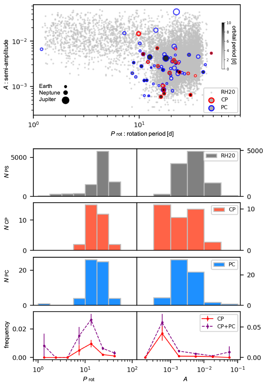
Figure 12: Distributions of periodic stars, planetary systems, and planetary candidates in $K2$ with respect to the stellar rotation period (left column) and semi-amplitude of the light curve (right column). Top to bottom; scatter plot of $A$ versus $P_{\rm rot}$; histograms of all periodic stars, confirmed planets (CP), and planetary candidates (PC); line graphs showing the frequencies of CP and CP + PC among all periodic stars, respectively. In the top panel, the sizes and colors to the sizes and orbital periods, respectively, of the targets flagged as CPs (red) or PCs (blue).

6.2 Implication to Current Planetary Systems

To understand the detection biases caused by stellar activity, we interpreted the current planetary distribution. We first constructed a scatter plot of $P_{\rm rot}$ vs. $A$ (top panel of Figure 12). Each gray dot is a periodic star (PS; i.e., a star showing photometric periodicity induced by the rotation) with an effective temperature between 3000 K and 4000 K in Campaigns 0 - 18 of the $K2$ mission measured in Reinhold & Hekker (2020) and each of these PSs may or may not host a planetary system. We also removed the stars belonging to typical clusters in K2, Hyades, Praesepe, Pleiades, Upper Scorpius, and $\gamma$ Ophiuchi, referring the EPIC list in the literatures (Rebull et al., 2016; Douglas et al., 2017; Rebull et al., 2018; Douglas et al., 2019) to focus on the matured planetary systems. The samples of Reinhold & Hekker (2020) require a match among the LS, the autocorrelation (McQuillan et al., 2013), and the wavelet analyses for determining their rotation periods (Torrence & Compo, 1998). The red- and blue-edged circles in the top panel of Figure 12 are the targets flagged as confirmed planets (CPs) and planetary candidates (PCs) in the ExoFOP (2019), where young CPs and PCs are removed as in the case of the PS. To obtain the rotation periods of the CPs and PCs, we ran the LS periodogram after masking the transit and eclipse signals and detrending as described in Section 3.2 with the K2SFF light curves. We determined the first independent peak as the rotation period for each target. The vertical axis of the graph is the semi-amplitude of the 5th - 95th photometric variation, equivalent to $R_{\rm var}/2$ in Reinhold & Hekker (2020) for the gray points. The middle three rows of Figure 12 histograms of PSs, CPs, and PCs with respect to $P_{\rm rot}$ (left panels) and $A$ (right panels); the bottom panels, plot the frequencies of CP and CP+PC to the PS [$N_{\rm CP}/N_{\rm PS}$ and $(N_{\rm CP}+N_{\rm PC})/N_{\rm PS}$, respectively] in each bin of the preceding histograms. The error values are calculated based on the binomial distribution, but are likely underestimated due to the small numbers of the CP and PC samples.

In the scatter plot, the CPs and PCs are distributed around $P_{\rm rot}$ $\sim 10$ and $A$ $\sim 10^{-3}$. The CP targets with long orbital periods tend to distribute around the lower right region of the plot. No CPs are found at rotation periods below five days. The size is positively correlated with $A$ among the PCs (less so among the CPs). The orbital photometry of Jupiter-sized targets can contaminate the stellar activity and make $A$ larger because such targets are often detected as false positives (FP) of eclipsing binaries (e.g., KOI-977; Hirano et al., 2015). One PC (EPIC 20192810.01) locates among the shortest $P_{\rm rot}$, but after visual inspection of the light curve, we concluded that EPIC 21092810.01 is an FP of stellar rotational activity.

The distributions of $N_{\rm CP}$ and $N_{\rm PC}$ are slightly shifted towards shorter $P_{\rm rot}$ than $N_{\rm PS}$. Consequently, the CPs and PCs are most commonly found from approximately 7 to 20 days, while this systematic feature is small among the CPs alone. Meanwhile, the CPs show a wider distribution of semi-amplitudes of the light curves $A$ than the PSs. The limited number of PSs in the low $A$ region might be attributed to the high requirement of the period determination in Reinhold & Hekker (2020). The occurrence frequencies of CP and PC appear to be high around low-activity stars with $A$ less than $10^{-3}$.

Compared with the systematic features above, the recovery rate in Figure 11 moderately vary as functions of $P_{\rm rot}$ and $A$. For the stellar rotation, while a peak locates at approximately 10 days in the frequencies of CPs and CPs + PCs (left bottom in Figure 12), the decrease of recovery rate between about 3 and 10 days is almost $20\%$ when the orbital period is 10 d (left bottom of $P_{\rm orb}=10$ d in Figure 11). The frequency of semi-amplitudes of the light curves rises suddenly to its maximum at $A\approx 10^{-3}$ (right bottom in Figure 12), but the decrease in detectability is moderate by around $60\%$ from $A=10^{-4}$ to $10^{-1}$ (right bottom for each $P_{\rm rot}$ in Figure 11). These frequency trends in Figure 12 indicate that a true planetary radius distribution rapidly changes while the detection efficiency gently changes with $P_{\rm rot}$ and $A$. Especially for $A$, many CPs and PCs are missing in the high amplitude region regardless of the selection biases of Reinhold & Hekker (2020).

Our results on the detectability of transiting signals simply suggest a low planet frequency around active cool stars intrinsically in the current observational data. This idea was originally proposed by McQuillan et al. (2013), who analyzed the first Kepler observational results. Rapid rotators in low-mass stars in matured age can be explained by decrease of the magnetic braking effect in the PMS phase and retention of rapid rotators after the ZAMS of M-dwarfs (Reiners & Mohanty, 2012), spin acceleration due to transportation of angular momentum by planetary migration or engulfment in host stars (Bolmont et al., 2012; Gallet & Delorme, 2019), or protoplanetary disk dissipation in the early stage due to the binarity of low-mass stars, which does not affect stellar rotation (Stauffer et al., 2018). To discuss relationships between the above scenarios and the lack of planets around rapidly rotators, further investigations of the planetary frequency in young stage are required.

7 Summary

We investigated the detectability of planetary candidates in the presence of photometric variations typically shown by young cool stars. The transit detectability was evaluated by making the SDE maps of the K2 light curves collected in the four clusters — Hyades, Praesepe, Pleiades, and Upper Scorpius — using the planetary transit model over a wide range of orbital periods and planetary radii. The systematic trends of the transit detectability were similar in each cluster. We concluded that the lack of planets in Pleiades (Gaidos et al., 2017) is likely due to rapid rotations of M-dwarfs around the ZAMS.

In addition, we showed that the detectability of young planets is improved by future photometric observations in the NIR, such as by the JASMINE mission (Gouda, 2018). For the targets with rotational periods around one day or smaller, the detectability at a threshold of $1\%$ transit depth was (at most) approximately $20\%$ higher at NIR wavelengths than at visible wavelengths. This improvement suggests that future NIR photometric monitoring will find planetary systems that were overlooked in the K2 or TESS missions and will constrain the scenarios of planetary and stellar activity evolution.

Comparing the recovery rate to the current planet frequency as functions of stellar activity, confirmed planets and candidates around M-dwarfs in the K2 mission are likely missing around active stars. Whereas more observational researches are required, this biased distribution may be an evidence that planet formation and/or evolution are prevented around rapid rotators in M-dwarfs. Follow-up observations at NIR wavelengths are expected to impose further constraints on roles of stellar activity in young planetary systems.

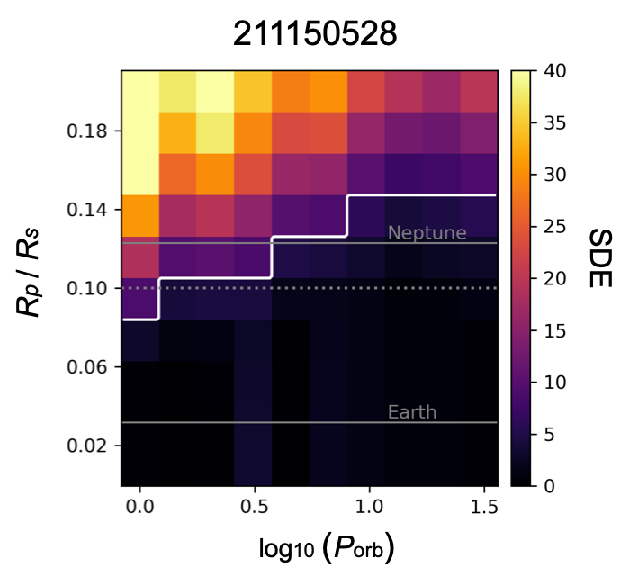
Figure 13: The SDE map for EPIC 211150528 which is a rapidly rotating target for comparison with lower panels of Figure 7 in Rizzuto et al. (2017).

Appendix A Uncertainty in the Estimation of Stellar Properties

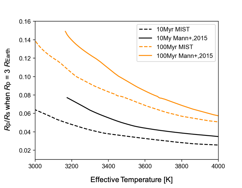
Figure 14: $T_{\rm eff}$ vs. $R_{\rm p}/R_{\rm s}$ plot when $R_{\rm p}=3R_{\oplus}$ with Mann et al. (2015) (solid) and the MIST (Dotter, 2016; Choi et al., 2016) (dashed) ; the black and orange lines are 10 Myr and 100 Myr, respectively.

We discuss the uncertainty in the stellar properties estimated with the empirical formula in Mann et al. (2015) (see Section 2 and 3.2), which is required since stellar radius in the PMS phase (10 - 100 Myr) is likely inflated. We calculate the $T_{\rm eff}$ vs. $R_{\rm s}$ plot using the MIST stellar isochrones (Dotter, 2016; Choi et al., 2016) with ages of 10 Myr and 100 Myr which correspond to the Upper Scorpius and Pleiades ages, respectively. The stellar radius is derived via the Stefan-Boltzmann law with the effective temperature and luminosity. To clarify how much effect the uncertainty has on our SDE estimations, we converted $R_{\rm s}$ into $R_{\rm p}/R_{\rm s}$ when $R_{\rm p}=3R_{\oplus}$ which corresponds to typical value of the vertical axis in Figure 2, and show the result in Figure 14. Our estimations with Mann et al. (2015) seem to be larger by about 0.02 in $R_{\rm p}/R_{\rm s}$ than with the MIST for both 10 Myr and 100 Myr, and this difference corresponds to about one pixel grid in the SDE maps. Therefore, we presumably overestimate the planet detectability in the Upper Scorpius and Pleiades by approximately 10 %, although this level of systematic error does not affect the overall results and conclusion discussed in the text.

Appendix B Comparison to Other Detrending Method

We discuss the efficiency of detrending method introduced in Section 3.3 comparing to other approaches. Firstly, Rizzuto et al. (2017) have developed two transit recovery algorithms called notch filter pipeline and Locally Optimized Combination of Rotation (LOCoR). The first one performs fitting a transit-shaped notch and quadratic baseline in a 0.5 or 1 d window to the stellar activity and transit dips simultaneously, and has sensitivity to targets with $P_{\rm rot}\geq 1-1.5$ d. The latter one models stellar variability by a linear combination of observed rotation periods for each target and is effective for the most rapid rotators with $P_{\rm rot}\leq 2$ d. As reference, Rizzuto et al. (2017) show results of their injection recovery test using both of these methods in their Figure 7 for EPIC 210892390 and EPIC 211150528. When focusing on better ones, detection borders lie in about 3 - 4 $R_{\oplus}$ for the notch filter to EPIC 210892390 and about 2.5 - 3.5 $R_{\oplus}$ for the LOCoR to EPIC 211150528. For comparison, we also show the SDE maps for EPIC 210892390 and EPIC 211150528 in Figure 2 and Figure 13, respectively. The boundaries exist in approximately 3.5 - 5 $R_{\oplus}$ and 2.5 - 4 $R_{\oplus}$ for EPIC 210892390 and EPIC 211150528, respectively, while we show them with planetary radii in $R_{\rm p}/R_{\rm s}$ and $P_{\rm rot}$ in log scale. These differences seem to be corresponding to a few pixels and negligible for the discussions.

Next, we discuss the efficiency of some detrending methods before the TLS (Hippke & Heller, 2019a). We tested the following five ways to detrend light curves for the three target with different rotation periods, EPIC 211000411, EPIC 210892390, and EPIC 210947895.

1. FFT filter + 1 d - median filter (performed in Section 3.3.)

2. FFT filter + 0.3 d - median filter

3. 0.3 d - median filter

4. 0.3 d - Tukey’s biweight filter (Tukey, 1977)

5. 0.3 d - Huber spline detrend (Huber, 1964)

The latter two methods which are based on the robust statistics are evaluated as ideal methods in Hippke et al. (2019). We employed W$\bar{\texttt{o}}$tan (Hippke et al., 2019), a comprehensive time-series detrending package implemented in Python for the biweight and Huber spline analyses. We injected a planet with the orbital $P_{\rm orb}$ of 10 d and $R_{\rm p}/R_{\rm s}$ of 0.05, 0.1, 0.15 for EPIC 211000411, EPIC 210892390, and EPIC 21097895, respectively. These planetary radii are selected around the detection boundary.

The results are shown in Figure 15. For each target, the top panel shows a light curve after subtraction of long-term modulation. From the second panel to the bottom, we display detrended light curves with the five methods above. We show total light curves, closeup view with 10 d - window, and the TLS periodogram from left to right. The horizontal dashed line in the TLS periodogram indicates detection threshold with SDE of 7. For EPIC 211000411 whose rotation period is 8.6 d, there is no significant differences around the first peak among the five methods. This is due to that photometric variations longer than a few days can be easily removed by 1 d - window scaled detrending. For EPIC 210892390 with the rotation period of 1.4 d, our FFT + 1d median shows lower SDE than the other methods, while the detection is significant. Because the periodogram of the FFT + 0.3 d median shows comparable SDE to that of the 0.3 d biweight and huber spline, this decline likely depends on the window size. Also, the red noise is predominant in the original light curve, it is not possibly caused by the rotational moduration. For EPIC 210947895, the most rapidly rotator with 0.2 d, only our approach successfully detected the transit signal. This indicates that the rotational noise could be removed in the FFT filtering and short window sized filtering may degenerate the red noise and transit signal. Thus, we conclude that our approach, the FFT + 1 d median, is likely more sensitive to extremely rapid rotators than other detrending methods and is appropriate when we discuss the lack of the planets around active stars. Note that discussion here is specific to the K2 light curves which contain about 50 data points in a 1 d sized bin. Because the TESS has a few hundreds of data points in similar time scale, the results will be different.

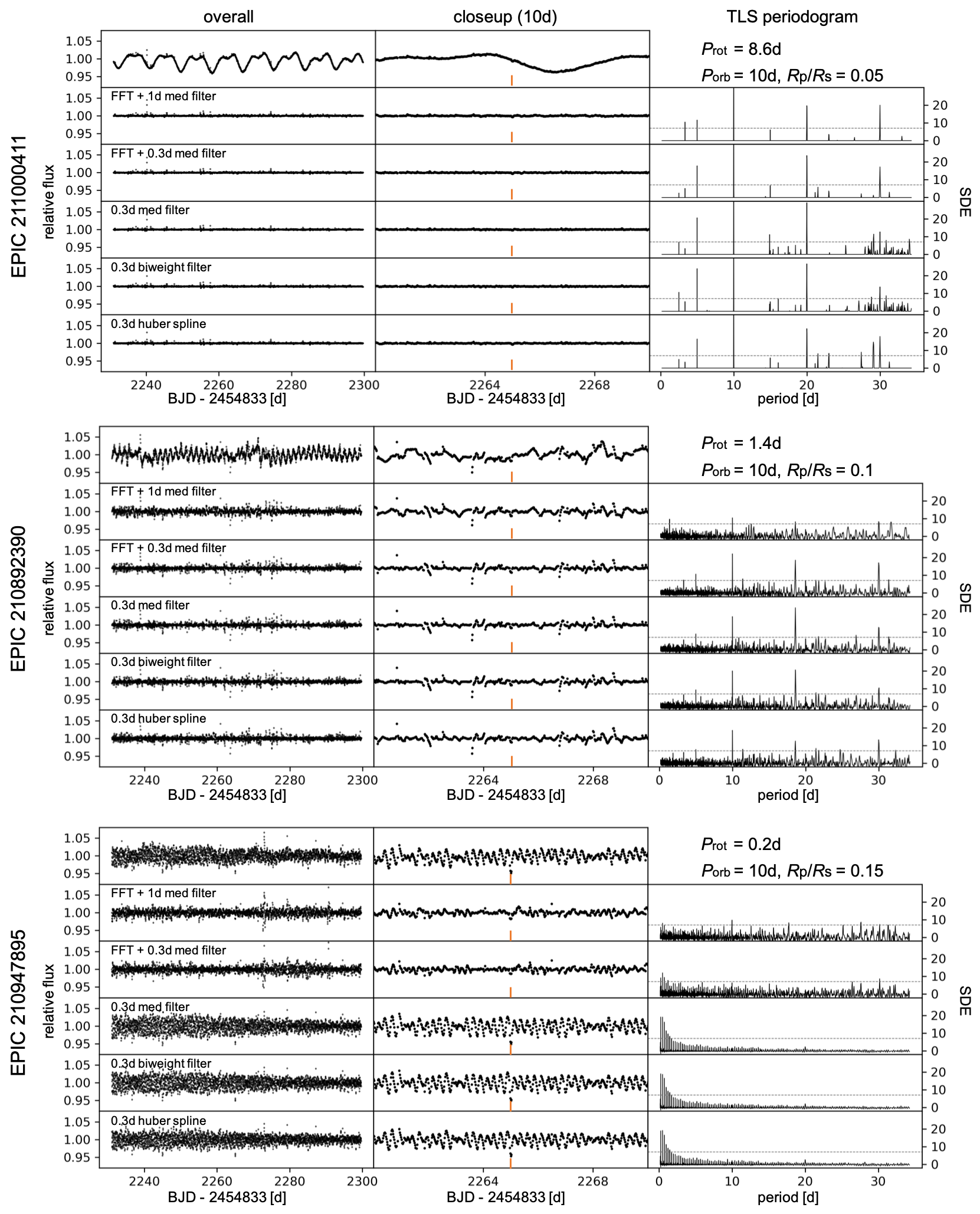
Figure 15: Light curves and TLS results for EPIC 211000411, EPIC 210892390, and EPIC 210947895. For each target, from the top to the bottom, light curve after subtraction of long-term modulation and light curve detrended with the FFT + 1 d median filtering, the FFT + 0.3 d median filtering, only the 0.3 d median filtering, the 0.3 d biweight filtering and the 0.3 Huber spline detrending; from the left to the right, overall and colseup view of light curves and the TLS periodogram. In the middle column, we indicate transit signals with orange line; in the right column, dashed horizontal line represents the SDE of 7.

Appendix C Validity of the 10 $\times$ 10 SDE map

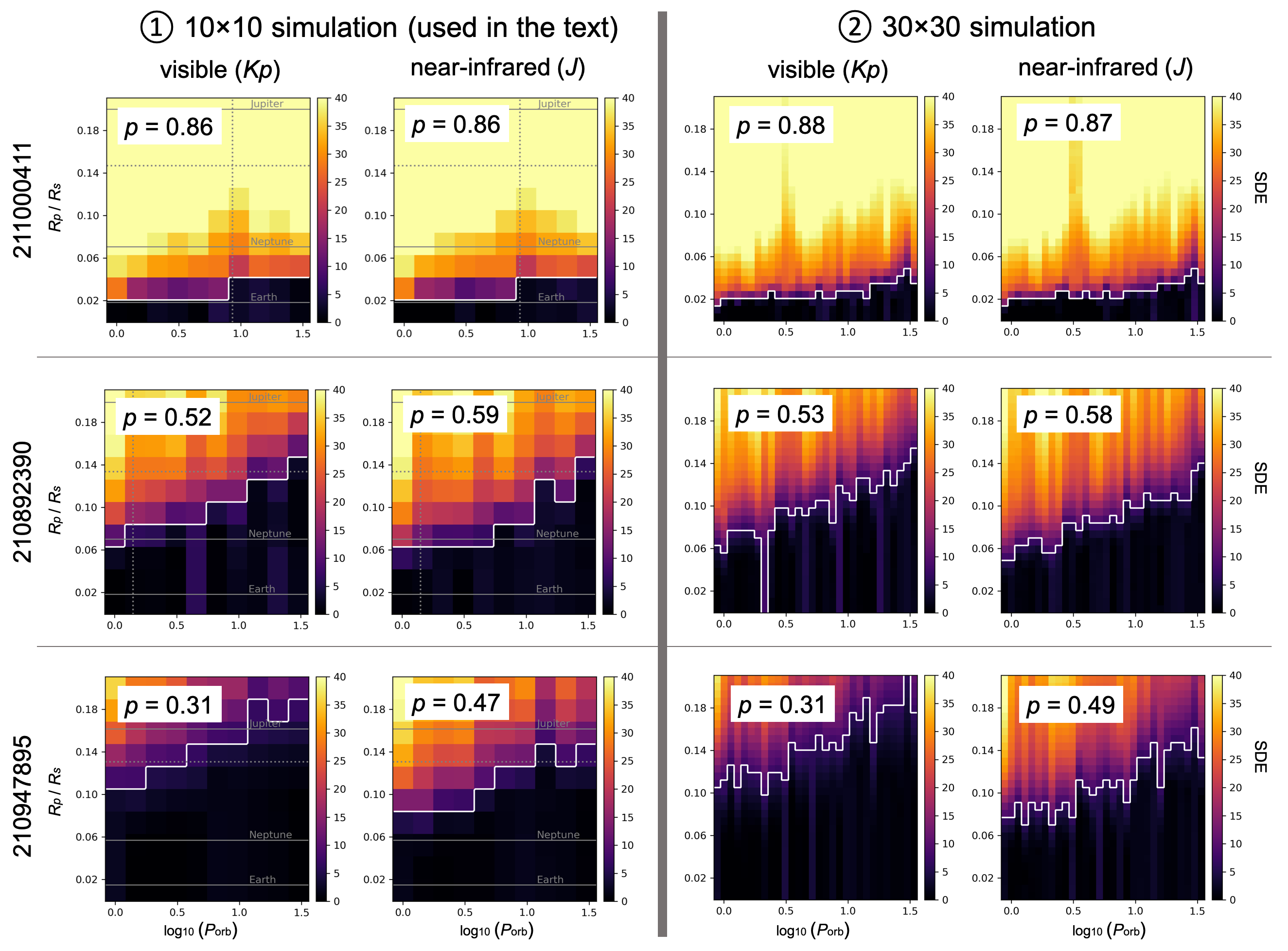
Figure 16: Comparisons of results between the 10 $\times$ 10 (Figure 2) and 30 $\times$ 30 simulations for EPIC 211000411, EPIC 210892390, and EPIC 210947895.

To ensure the validity of the 10 $\times$ 10 SDE maps in Section 3.2, we show a comparison for the typical three targets with simulation results with 30 $\times$ 30 grids in Figure 16. The left and right panels are the results of the 10 $\times$ 10 and 30 $\times$ 30 simulations, respectively. We show the recovery rate $p$ (see Section 4.2) in the left top of each panel. The $p$ almost agree within about 1% error, and features of the colormaps seem to be consistent between the two simulations. Thus, we conclude that the 10 % 10 simulations are sufficient for this study. There are some spikes on the SDE distribution. For example, $\log{P_{\rm orb}}=0.5$ in EPIC 211000411 and $\log{P_{\rm orb}}=0.3$ in EPIC 210892390 show systematically high values along the vertical axis. This might be caused by mis-detection of the transit signal in the TLS algorithm, because periodic residuals remain after the FFT filtering.

References

- Allard et al. (2013) Allard, F., Homeier, D., Freytag, B., et al. 2013, Memorie della Societa Astronomica Italiana Supplementi, 24, 128. https://arxiv.org/abs/1302.6559
- Barber et al. (2022) Barber, M. G., Mann, A. W., Bush, J. L., et al. 2022, arXiv e-prints, arXiv:2206.08383. https://arxiv.org/abs/2206.08383
- Benatti et al. (2019) Benatti, S., Nardiello, D., Malavolta, L., et al. 2019, A&A, 630, A81, doi: 10.1051/0004-6361/201935598
- Bolmont et al. (2012) Bolmont, E., Raymond, S. N., Leconte, J., & Matt, S. P. 2012, A&A, 544, A124, doi: 10.1051/0004-6361/201219645
- Borucki et al. (2010) Borucki, W. J., Koch, D., Basri, G., et al. 2010, Science, 327, 977, doi: 10.1126/science.1185402
- Bouma et al. (2020) Bouma, L. G., Hartman, J. D., Brahm, R., et al. 2020, AJ, 160, 239, doi: 10.3847/1538-3881/abb9ab
- Bouma et al. (2022a) Bouma, L. G., Curtis, J. L., Masuda, K., et al. 2022a, AJ, 163, 121, doi: 10.3847/1538-3881/ac4966
- Bouma et al. (2022b) Bouma, L. G., Kerr, R., Curtis, J. L., et al. 2022b, arXiv e-prints, arXiv:2205.01112. https://arxiv.org/abs/2205.01112
- Burke & McCullough (2014) Burke, C. J., & McCullough, P. R. 2014, ApJ, 792, 79, doi: 10.1088/0004-637X/792/1/79
- Cale et al. (2021) Cale, B. L., Reefe, M., Plavchan, P., et al. 2021, AJ, 162, 295, doi: 10.3847/1538-3881/ac2c80
- Choi et al. (2016) Choi, J., Dotter, A., Conroy, C., et al. 2016, ApJ, 823, 102, doi: 10.3847/0004-637X/823/2/102
- Ciardi et al. (2018) Ciardi, D. R., Crossfield, I. J. M., Feinstein, A. D., et al. 2018, AJ, 155, 10, doi: 10.3847/1538-3881/aa9921
- Claret & Bloemen (2011) Claret, A., & Bloemen, S. 2011, A&A, 529, A75, doi: 10.1051/0004-6361/201116451
- Collaboration (2020) Collaboration, G. 2020, Gaia Source Catalogue eDR3, IPAC, doi: 10.26131/IRSA541. https://catcopy.ipac.caltech.edu/dois/doi.php?id=10.26131/IRSA541
- Curtis et al. (2018) Curtis, J. L., Vanderburg, A., Torres, G., et al. 2018, AJ, 155, 173, doi: 10.3847/1538-3881/aab49c
- David et al. (2019) David, T. J., Petigura, E. A., Luger, R., et al. 2019, ApJ, 885, L12, doi: 10.3847/2041-8213/ab4c99
- David et al. (2016) David, T. J., Hillenbrand, L. A., Petigura, E. A., et al. 2016, Nature, 534, 658, doi: 10.1038/nature18293
- Dotter (2016) Dotter, A. 2016, ApJS, 222, 8, doi: 10.3847/0067-0049/222/1/8
- Douglas et al. (2017) Douglas, S. T., Agüeros, M. A., Covey, K. R., & Kraus, A. 2017, ApJ, 842, 83, doi: 10.3847/1538-4357/aa6e52
- Douglas et al. (2019) Douglas, S. T., Curtis, J. L., Agüeros, M. A., et al. 2019, ApJ, 879, 100, doi: 10.3847/1538-4357/ab2468
- Dressing & Charbonneau (2015) Dressing, C. D., & Charbonneau, D. 2015, ApJ, 807, 45, doi: 10.1088/0004-637X/807/1/45
- ExoFOP (2019) ExoFOP. 2019, Exoplanet Follow-up Observing Program - K2, IPAC, doi: 10.26134/EXOFOP2. https://catcopy.ipac.caltech.edu/dois/doi.php?id=10.26134/EXOFOP2
- Frasca et al. (2009) Frasca, A., Covino, E., Spezzi, L., et al. 2009, A&A, 508, 1313, doi: 10.1051/0004-6361/200913327
- Fukugita et al. (1995) Fukugita, M., Shimasaku, K., & Ichikawa, T. 1995, PASP, 107, 945, doi: 10.1086/133643
- Gaia Collaboration et al. (2020) Gaia Collaboration, Brown, A. G. A., Vallenari, A., et al. 2020, arXiv e-prints, arXiv:2012.01533. https://arxiv.org/abs/2012.01533
- Gaia Collaboration et al. (2016) Gaia Collaboration, Prusti, T., de Bruijne, J. H. J., et al. 2016, A&A, 595, A1, doi: 10.1051/0004-6361/201629272
- Gaidos et al. (2017) Gaidos, E., Mann, A. W., Rizzuto, A., et al. 2017, MNRAS, 464, 850, doi: 10.1093/mnras/stw2345
- Gallet & Delorme (2019) Gallet, F., & Delorme, P. 2019, A&A, 626, A120, doi: 10.1051/0004-6361/201834898
- Gilbert et al. (2022) Gilbert, E. A., Barclay, T., Quintana, E. V., et al. 2022, AJ, 163, 147, doi: 10.3847/1538-3881/ac23ca
- Godoy-Rivera et al. (2021) Godoy-Rivera, D., Pinsonneault, M. H., & Rebull, L. M. 2021, arXiv e-prints, arXiv:2101.01183. https://arxiv.org/abs/2101.01183
- Gouda (2018) Gouda, N. 2018, in Astrometry and Astrophysics in the Gaia Sky, ed. A. Recio-Blanco, P. de Laverny, A. G. A. Brown, & T. Prusti, Vol. 330, 90–91
- Hedges et al. (2021) Hedges, C., Hughes, A., Zhou, G., et al. 2021, AJ, 162, 54, doi: 10.3847/1538-3881/ac06cd
- Hippke et al. (2019) Hippke, M., David, T. J., Mulders, G. D., & Heller, R. 2019, AJ, 158, 143, doi: 10.3847/1538-3881/ab3984
- Hippke & Heller (2019a) Hippke, M., & Heller, R. 2019a, A&A, 623, A39, doi: 10.1051/0004-6361/201834672
- Hippke & Heller (2019b) —. 2019b, TLS: Transit Least Squares. http://ascl.net/1910.007
- Hirano et al. (2015) Hirano, T., Masuda, K., Sato, B., et al. 2015, ApJ, 799, 9, doi: 10.1088/0004-637X/799/1/9
- Howell et al. (2014) Howell, S. B., Sobeck, C., Haas, M., et al. 2014, PASP, 126, 398, doi: 10.1086/676406
- Huber (1964) Huber, P. J. 1964, The Annals of Mathematical Statistics, 35, 73 , doi: 10.1214/aoms/1177703732
- Klein & Donati (2020) Klein, B., & Donati, J. F. 2020, MNRAS, 493, L92, doi: 10.1093/mnrasl/slaa009
- Klein et al. (2022) Klein, B., Zicher, N., Kavanagh, R. D., et al. 2022, MNRAS, 512, 5067, doi: 10.1093/mnras/stac761
- Kopparapu et al. (2013) Kopparapu, R. K., Ramirez, R., Kasting, J. F., et al. 2013, ApJ, 765, 131, doi: 10.1088/0004-637X/765/2/131
- Kovács et al. (2002) Kovács, G., Zucker, S., & Mazeh, T. 2002, A&A, 391, 369, doi: 10.1051/0004-6361:20020802
- Livingston et al. (2018) Livingston, J. H., Dai, F., Hirano, T., et al. 2018, AJ, 155, 115, doi: 10.3847/1538-3881/aaa841
- Luger et al. (2016) Luger, R., Agol, E., Kruse, E., et al. 2016, AJ, 152, 100, doi: 10.3847/0004-6256/152/4/100
- Mann et al. (2015) Mann, A. W., Feiden, G. A., Gaidos, E., Boyajian, T., & von Braun, K. 2015, ApJ, 804, 64, doi: 10.1088/0004-637X/804/1/64
- Mann et al. (2016a) Mann, A. W., Gaidos, E., Mace, G. N., et al. 2016a, ApJ, 818, 46, doi: 10.3847/0004-637X/818/1/46
- Mann et al. (2016b) Mann, A. W., Newton, E. R., Rizzuto, A. C., et al. 2016b, AJ, 152, 61, doi: 10.3847/0004-6256/152/3/61
- Mann et al. (2017) Mann, A. W., Gaidos, E., Vanderburg, A., et al. 2017, AJ, 153, 64, doi: 10.1088/1361-6528/aa5276
- Mann et al. (2018) Mann, A. W., Vanderburg, A., Rizzuto, A. C., et al. 2018, AJ, 155, 4, doi: 10.3847/1538-3881/aa9791
- Mann et al. (2019) Mann, A. W., Dupuy, T., Kraus, A. L., et al. 2019, ApJ, 871, 63, doi: 10.3847/1538-4357/aaf3bc
- Mann et al. (2020) Mann, A. W., Johnson, M. C., Vanderburg, A., et al. 2020, AJ, 160, 179, doi: 10.3847/1538-3881/abae64
- Mann et al. (2021) Mann, A. W., Wood, M. L., Schmidt, S. P., et al. 2021, arXiv e-prints, arXiv:2110.09531. https://arxiv.org/abs/2110.09531
- Martioli et al. (2021) Martioli, E., Hébrard, G., Correia, A. C. M., Laskar, J., & Lecavelier des Etangs, A. 2021, A&A, 649, A177, doi: 10.1051/0004-6361/202040235
- McQuillan et al. (2013) McQuillan, A., Aigrain, S., & Mazeh, T. 2013, MNRAS, 432, 1203, doi: 10.1093/mnras/stt536
- Meibom et al. (2013) Meibom, S., Torres, G., Fressin, F., et al. 2013, Nature, 499, 55, doi: 10.1038/nature12279
- Miyakawa et al. (2021) Miyakawa, K., Hirano, T., Fukui, A., et al. 2021, AJ, 162, 104, doi: 10.3847/1538-3881/ac111d
- Morris et al. (2018) Morris, B. M., Agol, E., Davenport, J. R. A., & Hawley, S. L. 2018, ApJ, 857, 39, doi: 10.3847/1538-4357/aab6a5
- Nardiello (2020) Nardiello, D. 2020, MNRAS, 498, 5972, doi: 10.1093/mnras/staa2745
- Nardiello et al. (2021) Nardiello, D., Deleuil, M., Mantovan, G., et al. 2021, MNRAS, 505, 3767, doi: 10.1093/mnras/stab1497
- NASA Exoplanet Archive (2019) NASA Exoplanet Archive. 2019, Confirmed Planets Table, IPAC, doi: 10.26133/NEA1. https://catcopy.ipac.caltech.edu/dois/doi.php?id=10.26133/NEA1
- Newton et al. (2019) Newton, E. R., Mann, A. W., Tofflemire, B. M., et al. 2019, ApJ, 880, L17, doi: 10.3847/2041-8213/ab2988
- Newton et al. (2021) Newton, E. R., Mann, A. W., Kraus, A. L., et al. 2021, AJ, 161, 65, doi: 10.3847/1538-3881/abccc6
- Newton et al. (2022) Newton, E. R., Rampalli, R., Kraus, A. L., et al. 2022, arXiv e-prints, arXiv:2206.06254. https://arxiv.org/abs/2206.06254
- Obermeier et al. (2016) Obermeier, C., Henning, T., Schlieder, J. E., et al. 2016, AJ, 152, 223, doi: 10.3847/1538-3881/152/6/223
- Ohta et al. (2009) Ohta, Y., Taruya, A., & Suto, Y. 2009, ApJ, 690, 1, doi: 10.1088/0004-637X/690/1/1
- Owen (2019) Owen, J. E. 2019, Annual Review of Earth and Planetary Sciences, 47, 67, doi: 10.1146/annurev-earth-053018-060246
- Plavchan et al. (2020) Plavchan, P., Barclay, T., Gagné, J., et al. 2020, Nature, 582, 497, doi: 10.1038/s41586-020-2400-z
- Rebull et al. (2018) Rebull, L. M., Stauffer, J. R., Cody, A. M., et al. 2018, AJ, 155, 196, doi: 10.3847/1538-3881/aab605
- Rebull et al. (2016) Rebull, L. M., Stauffer, J. R., Bouvier, J., et al. 2016, AJ, 152, 113, doi: 10.3847/0004-6256/152/5/113
- Reiners & Mohanty (2012) Reiners, A., & Mohanty, S. 2012, ApJ, 746, 43, doi: 10.1088/0004-637X/746/1/43
- Reinhold & Hekker (2020) Reinhold, T., & Hekker, S. 2020, A&A, 635, A43, doi: 10.1051/0004-6361/201936887
- Ricker et al. (2015) Ricker, G. R., Winn, J. N., Vanderspek, R., et al. 2015, Journal of Astronomical Telescopes, Instruments, and Systems, 1, 014003, doi: 10.1117/1.JATIS.1.1.014003
- Rizzuto et al. (2017) Rizzuto, A. C., Mann, A. W., Vanderburg, A., Kraus, A. L., & Covey, K. R. 2017, AJ, 154, 224, doi: 10.3847/1538-3881/aa9070
- Rizzuto et al. (2018) Rizzuto, A. C., Vanderburg, A., Mann, A. W., et al. 2018, AJ, 156, 195, doi: 10.3847/1538-3881/aadf37
- Rizzuto et al. (2020) Rizzuto, A. C., Newton, E. R., Mann, A. W., et al. 2020, AJ, 160, 33, doi: 10.3847/1538-3881/ab94b7
- Scalo et al. (2007) Scalo, J., Kaltenegger, L., Segura, A. G., et al. 2007, Astrobiology, 7, 85, doi: 10.1089/ast.2006.0125
- Scargle (1982) Scargle, J. D. 1982, ApJ, 263, 835, doi: 10.1086/160554
- Skrutskie et al. (2003) Skrutskie, Cutri, M. F., Stiening, R. M., et al. 2003, 2MASS All-Sky Point Source Catalog, IPAC, doi: 10.26131/IRSA2. https://catcopy.ipac.caltech.edu/dois/doi.php?id=10.26131/IRSA2
- Stauffer et al. (2018) Stauffer, J., Rebull, L. M., Cody, A. M., et al. 2018, AJ, 156, 275, doi: 10.3847/1538-3881/aae9ec
- Torrence & Compo (1998) Torrence, C., & Compo, G. P. 1998, Bulletin of the American Meteorological Society, 79, 61, doi: 10.1175/1520-0477(1998)079<0061:APGTWA>2.0.CO;2
- Tukey (1977) Tukey, J. W. 1977, Exploratory data analysis
- Vanderburg & Johnson (2014) Vanderburg, A., & Johnson, J. A. 2014, PASP, 126, 948, doi: 10.1086/678764
- Vanderburg et al. (2018) Vanderburg, A., Mann, A. W., Rizzuto, A., et al. 2018, AJ, 156, 46, doi: 10.3847/1538-3881/aac894
- Wells et al. (2018) Wells, R., Poppenhaeger, K., Watson, C. A., & Heller, R. 2018, MNRAS, 473, 345, doi: 10.1093/mnras/stx2077