Black hole hierarchical growth efficiency and mass spectrum predictions

Abstract

Hierarchical mergers in bound gravitational environments can explain the presence of black holes with masses greater than $\sim 100M_{\odot}$. Evidence for this process is found in the third LIGO-Virgo-KAGRA gravitational-wave transient catalog (GWTC-3). We study the efficiency with which hierarchical mergers can produce higher and higher masses using a simple model of forward evolution of binary black hole populations in gravitationally bound systems like stellar clusters. The model relies on pairing probability and initial mass functions for the black hole population, along with numerical relativity fitting formulas for the mass, spin and kick speed of the merger remnant. If unequal mass pairing is disfavored, we show that the retention probability decreases significantly with later generations of the binary black hole population. Our model also predicts the distribution of masses of each black hole merger generation. We find that two of the subdominant peaks in the GWTC-3 component mass spectrum are consistent with second and third generation mergers in dense environments. With more binary black hole detections, our model can be used to infer the black hole initial mass function and pairing probability exponent.

1 Introduction

Understanding the formation channels of binary black holes (BBHs) is one of the primary science goals of gravitational wave (GW) astronomy. The proposed formation scenarios are broadly divided into two categories: isolated field binary evolution (Dominik et al., 2015; Belczynski et al., 2016; Woosley, 2016; Marchant et al., 2016; de Mink & Mandel, 2016) and dynamical binary formation in dense stellar environments (Portegies Zwart & McMillan, 2000; Miller & Lauburg, 2009; Downing et al., 2010; Rodriguez et al., 2015; Hurley et al., 2016; O’Leary et al., 2016; Rodriguez et al., 2016a, 2018; Petrovich & Antonini, 2017; Arca-Sedda & Gualandris, 2018; Fragione & Kocsis, 2018; Zevin et al., 2019). Of the $\sim$90 binary black holes reported in the third LIGO-Virgo-KAGRA (LVK) gravitational-wave transient catalog (GWTC-3) (Abbott et al., 2021a), a few binaries have at least one component’s mass in the “upper mass gap” (between $\sim 50\mbox{--}130M_{\odot}$). It is widely believed that this region is forbidden by stellar evolution due to pair-instability or pulsational pair-instability supernovae (Fowler & Hoyle, 1964; Barkat et al., 1967; Woosley, 2017; Farmer et al., 2019, 2020; Renzo et al., 2020; Marchant et al., 2018).

An alternate pathway to populate the upper mass gap is hierarchical assembly via multiple generations of BBH mergers (Fragione et al., 2018; Antonini et al., 2019; Fragione & Silk, 2020; Mapelli et al., 2021b; Britt et al., 2021; Banerjee, 2018). In this scenario progenitor black holes (BHs) do not originate directly from the collapse of massive stars, but rather from the remnants of previous generations of BBH mergers. Kimball et al. (2021) found evidence for hierarchical BBH mergers in the GWTC-2 catalog. Because BBH mergers generically result in GW recoil (Fitchett, 1983; Favata et al., 2004), this requires an astrophysical environment (such as a star cluster) with a sufficiently large escape speed to retain the merger remnants (Merritt et al., 2004; Gerosa & Berti, 2017). Nuclear star clusters (NSCs) and gaseous active galactic nuclei (AGN) disks are the most promising sites for repeated mergers due to their larger escape speeds (Antonini & Rasio, 2016; Antonini & Gieles, 2020; Mapelli et al., 2021a; McKernan et al., 2012; Bartos et al., 2017; McKernan et al., 2018). However, a subclass of globular clusters (GCs) may also facilitate hierarchical mergers of BBHs (Mahapatra et al., 2021; Antonini et al., 2022). Repeated mergers also offer a natural explanation for the existence of intermediate mass black holes of a few hundred solar masses (Miller & Hamilton, 2002).

Previous works studied the observed BH remnant retention probability using numerical relativity (NR) fitting formulas (Mahapatra et al., 2021; Doctor et al., 2021) and the properties of second or higher generation BHs (e.g., the mass ratio, chirp mass, spin magnitudes, effective spin parameter, etc.; Gerosa & Berti 2017, 2019; Gerosa et al. 2021; Fishbach et al. 2017; Doctor et al. 2019). It was found that the characteristics of different BH merger generations are largely governed by the relativistic orbital and merger dynamics rather than the astrophysical environments in which they merge (see Gerosa & Fishbach 2021 for a review of this topic). However, models of hierarchical mergers must consider the astrophysical environment’s efficiency at retaining post-merger remnants, to ensure they are available for next generation mergers. The main goal of this work is to develop a simple model that investigates the hierarchical merger process, especially when BH kicks are considered. We use this model to examine the cluster retention of BH merger remnants and the binary component mass distribution; these are computed as a function of the merger generation and the properties of the first-generation progenitor population.

Recently Zevin & Holz (2022) studied the impact of the host environment on the mass distributions of hierarchically-assembled BHs. They generate merger trees that start with first-generation (1g) BH seeds, and grow them by merging BHs in series while estimating the remnants properties using NR fits (Gerosa & Kesden, 2016). They do this for three different kinds of binary mergers: 1g+Ng, Ng+Ng, and Mg+Ng, with $\rm M\leq N$. Here Ng refers to the BH generation. For example, a 1g+1g merger produces a 2g remnant, which can then form a binary with a new 1g BH (1g+2g), another 2g BH (2g+2g), or with a higher generation BH (e.g., 2g+3g; see Fig. 1). Zevin & Holz (2022) found that once the escape speed of the host environment reaches $\sim 300\,\text{km/s}$, the fraction of hierarchically-assembled binaries with total masses greater than $100M_{\odot}$ exceeds the observed upper limit of the LVK mass distribution (see Fig. 4 of Zevin & Holz 2022). They argued that hierarchical formation in such environments should be inhibited by some unknown mechanisms to avoid this conflict.

Figure 1: A schematic depiction of the hierarchical merger process. First generation progenitor BHs form from stellar collapse. A fraction of that seed population form the first generation BBHs (1g+1g). If their merger remnants are retained by their environment (i.e., not ejected via GW recoil), they enter the 2g progenitor BH population. A fraction of the 2g population then forms binaries with other 2g BH remnants or with members of the 1g population. The subsequent merger remnants that are retained form the 3g progenitor population, which can then form 1g+3g, 2g+3g, and 3g+3g binaries. The diagram shows the process up to the formation of the 4g progenitor population.

Modeling repeated mergers in star clusters via full N-body simulations, while more accurate, is computationally expensive to explore. Here we propose a simple model for the evolution of the BBH population in a bound environment like a star cluster. We study the efficiency of hierarchical BH growth by calculating the retention probability of BBH remnants produced by different merger generations, accounting for the cluster escape speeds. This allows us to infer the properties of later BBH generations, such as their retention probabilities and mass distributions. These can be computed as a function of the pairing probability function (introduced in Pinsonneault & Stanek 2006; Kouwenhoven et al. 2009; Fishbach & Holz 2020) and the mass and spin distributions of the first generation progenitor BHs.

2 Model assumptions

Given the component masses and spin vectors of the BBH components, our model uses NR fitting formulas to predict the final mass, final spin, and kick imparted to the merger remnant due to the radiated GW energy, angular momentum, and linear momentum (Campanelli et al., 2007; Lousto & Zlochower, 2008; Lousto et al., 2012; Lousto & Zlochower, 2013; Barausse et al., 2012; Hofmann et al., 2016). To analyze a population of BBHs, these NR fits are supplemented with an initial mass function for the primary BH mass $m_{1}$ and a pairing probability function $p^{\rm pair}(q)$. The pairing probability phenomenologically determines the probability of forming a BBH with mass ratio $q(\equiv m_{2}/m_{1}\leq 1)$ in a particular cluster environment (Kouwenhoven et al., 2009; Fishbach & Holz, 2020). These ingredients allow one to set up and forward evolve the population through multiple generations of mergers.

Our model starts with a population of BHs in a bound environment that, for simplicity, we refer to as a cluster. This might be a GC, a NSC, or an AGN disk. The cluster is described solely by its escape speed $V_{\rm esc}$ in our model. The initial “first generation” (1g) BH population is described completely by their initial mass and spin distributions. We then pair these 1g BHs via a pairing probability function $p^{\rm pair}(q)$ to form a population of bound BBHs. (The details are described further below.) The mass, spin, and kick of the resulting BH merger remnants from this population are determined via NR fitting formulas.

Figure 1 provides a schematic illustration of how our model evolves the BH population. A cluster retains a merger remnant if its kick speed $V_{\rm kick}$ is less than the cluster’s escape speed. Hence, the first iteration of our model produces a subpopulation of second generation (2g) BHs (i.e., 1g+1g merger remnants) that are retained by the cluster. These 2g BHs are subsequently paired up with either 1g BHs or other 2g BHs. The second iteration of our model produces 3g progenitor BHs (retained products of 1g+2g or 2g+2g mergers). A third iteration produces 4g progenitor BHs (via 1g+3g, 2g+3g or 3g+3g mergers); and so on as the model is iterated further. Our goal is to study—as a function of the merger generation—the fraction of binaries retained in clusters and the properties of the remnant BH population (especially its mass distribution).

Our model makes the following assumptions about the mass and spin distributions of the 1g BH population and the pairing probability function.

Mass distribution: The mass of 1g progenitor BHs is assumed to follow a power-law distribution with a smooth tapering at the lower end of the distribution (Kroupa, 2001; Talbot & Thrane, 2018):

$$p(m)\propto{m}^{-\alpha}\ S(m|{m_{\rm min}},\delta_{m})\mathcal{H}({m_{\rm max}-m}),$$ (1)

where $\mathcal{H}$ is the Heaviside step function and $m_{\rm min}$ and $m_{\rm max}$ are the minimum and maximum masses of the power-law component of the 1g progenitor BH mass. Instead of a step-function at the low-mass end of the BH mass spectrum, we use a smoothing function $S(m\mid{m_{min}},\delta_{m})$ (Talbot & Thrane, 2018) which smoothly rises from 0 to 1 over the interval $(m_{\rm min},m_{\rm min}+\delta_{m})$:

$$S(m\mid{m_{\rm min}},\delta_{m})=\begin{cases}0\,,\;\text{for}\;\;m<{m_{\rm min}}\,,\\ \\ \frac{1}{f(m-{m_{\rm min}},\delta_{m})+1}\,,\;\\ \;\;\text{for}\;\;{m_{\rm min}}\leq m<{m_{\rm min}}+\delta_{m}\,,\\ \\ 1\,,\;\;\text{for}\;\;m\geq{m_{\rm min}}+\delta_{m}\,,\end{cases}$$ (2)

with

$$f(m^{\prime},\delta_{m})={\rm exp}\left(\frac{\delta_{m}}{m^{\prime}}+\frac{\delta_{m}}{m^{\prime}-\delta_{m}}\right).$$ (3)

Note that $\delta_{m}=0$ recovers the distribution with a sharp cut-off at $m_{\rm min}$. The spectral index $\alpha$ and the tapering parameter $\delta_{m}$ fully define the mass distribution of 1g progenitor BHs. We have chosen $\alpha=2.3$, corresponding to the Kroupa initial mass function (Kroupa, 2001), and $\delta_{m}=4.83$ as inferred from the GWTC-3 population (Abbott et al., 2021b). We set $m_{\rm min}=5M_{\odot}$ and $m_{\rm max}=50M_{\odot}$, motivated by the lower (Bailyn et al., 1998; Özel et al., 2010; Belczynski et al., 2012) and upper (Woosley, 2017; Farmer et al., 2020) mass gaps. Strictly speaking, the BH mass function in stellar clusters could depend on quantities such as metallicity (Chattopadhyay et al., 2022) that we have not incorporated here and that could have some effect on our conclusions.

Spin distribution: We consider two types of distributions for the dimensionless spin magnitude $\chi$ of a 1g BH: (i) a uniform distribution, where spin magnitudes of 1g BHs are drawn uniformly from the range $\chi\in[0,0.99]$ (see Sec. 2.4 of Antonini & Rasio 2016); and (ii) a beta distribution (Wysocki et al., 2019; Abbott et al., 2019) with mean $\mu_{\chi}=0.28$ and variance $\sigma^{2}_{\chi}=0.03$ (Abbott et al., 2021b). Spin tilt angles for all BH generations and population models are isotropically drawn over a sphere (Rodriguez et al., 2016b; Tagawa et al., 2020). However, when we consider the GWTC-3 population as our 1g progenitors, the spin tilt angles for 1g BHs are drawn from a mixture population of the isotropic and Gaussian distributions (Talbot & Thrane, 2017); this follows the “Default” spin model in Abbott et al. (2019). In that case, higher generation BHs spin tilt angles are again isotropically distributed over a sphere. Note that spin tilt angles are chosen at binary separations $\sim 10M$ where NR simulations typically start (see Barausse & Rezzolla 2009 and Sec. 2.1 of Gerosa & Sesana 2015).

Pairing probability function: The pairing probability depends only on the mass ratio via (Fishbach & Holz, 2020)

$${}p^{\rm pair}(q)\propto q^{\beta}\,,$$ (4)

where $\beta$ is the sole parameter that governs the pairing probability between two BHs in a cluster. The normalization factor depends on $m_{\rm min}$ and $m_{\rm max}$. Though simple, the form (4) is naturally expected as the mass ratio distribution is one of the unique signatures of any formation mechanism. It assumes that the cluster properties (i.e., $V_{\rm esc}$) do not evolve over the timescale of the entire hierarchical merger process; although, in reality, the pairing probability may depend on the cluster’s metallicity as well as its dynamical age (Chattopadhyay et al., 2022; Antonini & Gieles, 2020).

Our model also assumes that mutli-body interactions play a negligible role in ejecting BHs and altering the fraction of BHs that are retained. The position of the BBH within the cluster, along with any sinking due to dynamical friction, are likewise ignored. Inclusion of these effects will reduce the efficiency of hierarchical mergers; hence our estimates should be seen as upper limits.

We consider three values of $\beta$: 1.08 (inferred from the GWTC-3 population, Abbott et al. 2021b), 0, and $-1$. Choosing $\beta>0$ favors the formation of comparable-mass binaries; $\beta<0$ favors the formation of asymmetric binaries; $\beta=0$ corresponds to random pairing (Kouwenhoven et al., 2009). We choose $\beta=-1$ as a representative value for the asymmetric binary formation case (although this choice is somewhat ad-hoc).

Dynamical interactions in dense clusters produce more equal-mass mergers (see Sec. IVB and Fig. 9 of Rodriguez et al. 2016b). For binary-single and binary-binary encounters in dense clusters, binaries are prone to exchanging components, preferentially expelling less-massive components in favor of more massive companions (Sigurdsson & Hernquist, 1993). Binaries merging in AGN disks typically have lower mass ratios (see Fig. 3 of Yang et al. 2019, and Figs. 3 & 5 of Li 2022) as migration traps within AGN disks give rise to random pairing and hence more unequal-mass binaries (McKernan et al., 2012; Bellovary et al., 2016). Our choices of $\beta$ cover these two different types of dynamical interactions. The values $\alpha=3.4$ and $\beta=1.08$ are inferred from the GWTC-3 BBH population when analyzed with the Power-law + Peak mass model (Abbott et al., 2021b).

3 Evolving the BBH population

Figure 2: Retention probabilities as a function of cluster escape speed for different kinds of merger remnants. The different curves in each panel indicate the various possible binary merger combinations (i.e., 1g+2g, 2g+2g, etc.; see top legend.) Each panel uses different population model assumptions for the 1g progenitors. The retention probability of a particular merger remnant type is computed directly from the kick CDF of that population as discussed in the text and Appendix A. Retention probability decreases as we go from first generation mergers to higher generation mergers. For mergers that involve a particular generation, unequal mass binaries have higher retention probabilities than equal mass binaries (e.g., $\rm{P_{13}^{ret}}>\rm{P_{23}^{ret}}>\rm{P_{33}^{ret}}$, where $\rm P^{\rm ret}_{\rm MN}$ refers to the retention probability of the remnant of a Mg+Ng binary merger). Retention probabilities for different merger generations is relatively higher for formation scenarios that prefer asymmetric pairing ($\beta=-1$ panels). The errors due to sampling on the retention probability are of the $\mathcal{O}(10^{-3}-10^{-4})$ with 90% credibility based on 100 realizations.

To evolve our BBH population we begin by randomly drawing $\sim 10^{6}$ BH pairs from the previously described mass and spin distributions. Each pair is characterized by mass and spin parameters {$m_{1}^{\rm 1g}$, $m_{2}^{\rm 1g}$, $\boldsymbol{\chi}_{1}^{\rm 1g}$, $\boldsymbol{\chi}_{2}^{\rm 1g}$}, with “1” denoting the heavier “primary.” A pool of 1g+1g binaries inside a cluster with escape speed $V_{\rm esc}$ is then constructed by sampling over these pairs with a weight proportional to $p^{\rm pair}$ using Eq. (4).

We then estimate the final mass $M_{\rm f}$, spin $\chi_{\rm f}$, and kick $V_{\rm kick}$ of each binary’s merger remnant using NR fits. (These fits are developed in Barausse et al. 2012; Hofmann et al. 2016; Campanelli et al. 2007 and are summarized in Sec. V of Gerosa & Kesden 2016; see also Appendix A of Mahapatra et al. 2021). This produces the first generation (1g+1g) merger remnants. If a 1g+1g remnant is retained in the cluster, it can take part in further mergers. The necessary condition for the retention of a remnant in a cluster is that the GW kick imparted to the remnant should be less than the escape speed of the host cluster ($V_{\rm kick}<V_{\rm esc}$). Hence, the probability of repeated mergers in a cluster is directly proportional to the retention probability (the probability that a member of the population has $V_{\rm kick}<V_{\rm esc}$). Mahapatra et al. (2021) estimated the retention probability of GWTC-2 BBH events inside clusters with different escape speeds via the cumulative distribution function (CDF) of the kick posteriors (see Sec. 2 of Mahapatra et al. (2021)). Here the retention probability of 1g+1g mergers is calculated from the kick CDF of the population of 1g+1g merger remnants. The retention probability for 1g+1g remnants (and for future merger generations) can then be quantified as a function of the cluster escape speed. The retained 1g+1g remnants will produce the population for the second generation (2g) progenitor BHs.

There are two possibilities for second generation mergers: 1g+2g or 2g+2g binaries that are formed according to the pairing probability function. The properties and retention probabilities of the resulting mergers are computed as described above, with further details in Appendix A. The retained remnants form the third generation (3g) progenitor population. From there, the third generation of binaries is paired via three possible combinations: 1g+3g, 2g+3g, and 3g+3g. The subpopulation that is retained after these 3g binaries merge forms the 4g progenitor BH population. In principle, this process goes on until there are no more BHs left in the cluster and/or inefficiency in pairing halts the process. Considering the limited number of high-mass BHs in the current LVK observational sample, we stop our iteration when 4g progenitor BHs are formed.

We consider six models with $\alpha=2.3$, $\beta=(1.08,0,1)$, and spins following a uniform or Beta distribution. For each parameter choice we evolve the corresponding population, tracking the properties of every possible merger generation. We also forward evolve the GWTC-3 population according to our model (taking the GWTC-3 binaries as our 1g+1g binaries). Appendix A describes the steps of the forward evolution in an algorithmic way.

4 Efficiency of hierarchical mergers

We study the retention probability for six different kinds of mergers as a function of a cluster’s escape speed. NR fits tell us that the remnant BH recoil speeds are relatively low for binaries with relatively unequal masses and small component spins; hence, such binaries will have higher retention probabilities.

Figure 2 shows retention probability versus cluster escape speed for different kinds of mergers. That figure suggests that a cluster with a $500$ km/s escape speed has a retention probability between 35% and 85%, depending on the merger type and the assumptions about the 1g progenitor population. Among mergers that involve a particular generation (e.g., 2g+2g and 1g+2g, which both have 2g BHs as components), unequal mass mergers have higher retention probabilities than equal mass mergers. For example, in second generation mergers 1g+2g mergers have higher retention probability than 2g+2g mergers. This is due to the lower kick speeds in asymmetric BBH mergers. We find that the retention probabilities of merger remnants fall off as we proceed from first generation mergers to higher generation mergers. But if the cluster dynamics prefers the pairing of asymmetric mass binaries (i.e., $\beta=-1$), then the retention probabilities for later generation mergers become higher, and hierarchical mergers become more efficient. However, as the cluster ages most of the 1g BHs are converted to higher generation BHs via mergers. So, for example, fewer 1g BHs will be available to merge with a 3g BH. The evolution of a cluster would, therefore, make such mergers rare and inefficient.

A crucial question is how abundant are the star clusters that have escape speeds of at least $500$ km/s. From current observations the escape speed distributions at present-day ($z=0$) for GCs and NSCs peak at $\sim 30$ km/s and $\sim 150$ km/s respectively (Antonini & Rasio, 2016; Georgiev et al., 2016; Harris, 1996). (See Fig. 3 of Antonini & Rasio 2016; note that these escape speed estimates are from the cluster center for GCs, whereas for NSCs they are defined at the half-mass cluster radius.) Using those present-day escape speed distributions, we find that the retention probability of merger remnants falls off from $\sim 25\%$ $(\sim 1\%)$ to $\sim 10\%$ ($\sim 0.4\%$) as we proceed from first generation mergers to higher generation mergers in NSCs (GCs). However, star clusters were more massive and denser at higher redshifts, and the corresponding higher escape speeds will increase the retention probability. For instance, at birth GCs have masses that are on average a factor of $\sim 4.5$ times larger than their present day masses (Webb & Leigh, 2015), increasing their escape speeds by a factor $\sim\sqrt{4.5}$.

Figure 3: The mass distribution of the primary binary component. The colored curves show the different generations of BBH mergers computed via our model; the black curve shows the observed GWTC-3 population. The escape speed of the cluster is assumed to be $500\,{\rm km/s}$ in our model; we have verified that this assumption has no visible impact on the model predictions. The inset shows a zoomed-in version of the plot highlighting the subdominant peaks. Note that the mass distributions are normalized individually. Therefore the relative heights between them carry no information. The sampling error on the y-axis values are of order $\mathcal{O}(10^{-3}-10^{-6})$ (with 90% credibility and based on 100 realizations), and are hence not shown.

Table 1: Fraction of each binary merger type contributing to the peaks in the primary mass distribution. The first column indicates the primary component mass ranges corresponding to the first, second, and third peaks in Fig. 3. The second column lists the binary merger type. The third column is the fraction of the indicated merger type that contributes to a given primary mass range. Numbers in bold indicate the mass range where a given merger type makes its dominant contribution. The error on each fraction is due to sampling noise (within 90% credibility and based on 100 realizations).

Primary mass range	Merger type	Fraction
$5M_{\odot}-13M_{\odot}$	1g+1g	$\textbf{0.5734}^{+0.0023}_{-0.0023}$
	1g+2g	$0.1348^{+0.0039}_{-0.0039}$
	2g+2g	$0.0308^{+0.0019}_{-0.0019}$
	1g+3g	$0.0003^{+0.0002}_{-0.0002}$
	2g+3g	$0.0000^{-0.0000}_{+0.0000}$
	3g+3g	$0.0000^{-0.0000}_{+0.0000}$
$13M_{\odot}-25M_{\odot}$	1g+1g	$0.2956^{+0.0029}_{-0.0023}$
	1g+2g	$\textbf{0.5893}^{+0.0056}_{-0.0046}$
	2g+2g	$\textbf{0.5349}^{+0.0062}_{-0.0068}$
	1g+3g	$0.2405^{+0.0057}_{-0.0074}$
	2g+3g	$0.1715^{+0.0051}_{-0.0050}$
	3g+3g	$0.0475^{+0.0028}_{-0.0026}$
$25M_{\odot}-44M_{\odot}$	1g+1g	$0.1149^{+0.0017}_{-0.0017}$
	1g+2g	$0.2208^{+0.0039}_{-0.0036}$
	2g+2g	$0.3069^{+0.0056}_{-0.0050}$
	1g+3g	$\textbf{0.5758}^{+0.0086}_{-0.0060}$
	2g+3g	$\textbf{0.5483}^{+0.0060}_{-0.0063}$
	3g+3g	$\textbf{0.5434}^{+0.0076}_{-0.0099}$

5 Predicted mass distribution

Our model also predicts the mass spectrum of various BH generations as a function of the model parameters. This allows us to compare our model predictions with the GWTC-3 results. Figure 11 of Abbott et al. (2021b) shows the mass spectrum of the primary in GWTC-3 inferred by different models. For convenience, we focus on the Flexible Mixture model framework (FM; Tiwari 2022, 2021) discussed there; we plot our predictions along with that of FM (solid black) in Fig. 3.

The FM, which is fitted with the GWTC-3 events, predicts multiple peaks in the component mass spectrum. This was first identified in the GWTC-2 population (Abbott et al., 2021c) by Tiwari & Fairhurst (2021). The dominant peak occurs at $\sim 10M_{\odot}$, with two subdominant peaks at $\sim 15M_{\odot}$ and $\sim 35M_{\odot}$ (see Fig. 11 of Abbott et al. 2021b). Intriguingly, the dominant peak is consistent with the 1g+1g mergers of our model. The secondary and tertiary peaks are consistent with mergers involving 2g (1g+2g and 2g+2g mergers) and 3g (1g+3g, 2g+3g, and 3g+3g mergers) BHs, respectively. These curves assume a uniform spin distribution; but we have verified that using a beta distribution for the spins does not produce any visible change in the plot. We also find similar features when we compare the chirp mass distribution of the GWTC-3 population (Fig. 2 of Abbott et al. 2021b) with the chirp mass distribution of higher generation mergers as predicted by our model. Our model also reproduces the component spin magnitude and effective spin distributions of Gerosa & Berti (2017); Fishbach et al. (2017); Gerosa et al. (2021). The mass ratio distribution from our model, which plays a crucial role in determining the pairing probability of binaries, is discussed further in Appendix B and Fig. 4 therein.

Under the assumption that the distinct peaks in the observed component mass spectrum arise from different generations of mergers, our model can be used to quantify the contribution of each merger type to the observed mass spectrum. To do this, we consider three mass ranges that broadly capture the first, second, and third peaks: $5M_{\odot}\mbox{--}13M_{\odot}$, $13M_{\odot}\mbox{--}25M_{\odot}$, and $25M_{\odot}\mbox{--}44M_{\odot}$. The fractions of Mg+Ng mergers that lie inside these mass ranges are shown in Table 1. We find that $57\%$ of the 1g+1g BBHs have primary masses between $5M_{\odot}\mbox{--}13M_{\odot}$, while $59\%$ of the 1g+2g mergers and $53\%$ of the 2g+2g mergers have primary masses in the range $13M_{\odot}\mbox{--}25M_{\odot}$. At the same time, $58\%$ of the 1g+3g mergers, $55\%$ of the 2g+3g mergers, and $54\%$ of the 3g+3g mergers have primary masses within the $25M_{\odot}\mbox{--}44M_{\odot}$ mass range. According to our model, this suggests that the first peak is dominated by 1g+1g mergers, the second is dominated by 1g+2g and 2g+2g mergers, and the third peak is dominated by 1g+3g, 2g+3g and 3g+3g mergers. For instance, our model interprets GW190412 (Abbott et al., 2020) as a 1g+3g merger which is consistent with the findings of Rodriguez et al. (2020).

Despite the small sample size of the currently observed BBH population ($\sim 90$ BBH mergers), these findings strongly suggest that the multiple peaks in the observed mass spectrum could originate from different generations of mergers. With the detections of several hundred BBHs in future observing runs, these peaks, if real, will be much better resolved, allowing a more precise vetting of the model predictions. More detections will help to infer the values of the $\alpha$ and $\beta$ power-law exponents. These are fundamental quantities that govern the formation and pairing of BHs in dynamical formation scenarios.

6 Conclusion

We have proposed a computationally inexpensive method to study the forward evolution of the binary black hole population. The model predicts the mass distributions of various generations of BH mergers, which we compared against the GWTC-3 results. We find a generic model with $\alpha=2.3$ and $\beta=1.08$ reproduces the dominant and subdominant peaks in the primary mass spectrum of the GWTC-3 sample. The subdominant peaks can be explained as resulting from mergers of second and third generation mergers as proposed in Tiwari & Fairhurst (2021).

Future GW observations could subject this model to more stringent tests. In addition to better resolving the subdominant peaks in the mass spectrum, the relative peak heights carry additional information, such as the delay time distribution of BBHs in clusters. This could be explored with a larger observational sample from future LVK observing runs. Future BBH catalogs may also allow direct inference of the $\alpha$ and $\beta$ parameters entering the model, shedding light on fundamental quantities in stellar physics (the initial mass function of BHs) and BH cluster dynamics (the pairing probability function).

Appendix A Summary of our BBH population evolution scheme

Here we provide additional details and a step-by-step schematic procedure illustrating how we form binary black holes, pair them, and forward evolve the binary population.

1. Using the 1g BH mass [see Eq. (1)] and spin distributions as described in Sec. 2, we draw a set of 1g BH mass values $\{M_{j}\}$ and spin values $\{{\bm{\chi}}_{j}\}$, where $j=1\ldots 2N$ and $N\sim 10^{6}$. This yields a set of unpaired 1g BHs characterized by their masses and spins $\Theta_{j}^{\rm 1g}=[M_{j},{\bm{\chi}_{j}}]$,

   $${}\{\Theta_{j}^{\rm 1g}\}=\{\Theta_{1}^{\rm 1g},\Theta_{2}^{\rm 1g},\ldots,\Theta_{2N}^{\rm 1g}\}\,.$$ (A1)

2. These BHs are now randomly paired to create a list of $N$ 1g+1g BH/BH pairs with parameters

   $${}\{\theta_{i}^{\rm 1g+1g}\}=\{\theta_{1}^{\rm 1g+1g},\theta_{2}^{\rm 1g+1g},\ldots,\theta_{N}^{\rm 1g+1g}\}\,,$$ (A2)

   where $\theta_{i}^{\rm 1g+1g}=[M^{(i)}_{1},M^{(i)}_{2},{\bm{\chi}}_{1}^{(i)},{\bm{\chi}}_{2}^{(i)}]$ are the parameters for the $i^{\rm th}$ 1g+1g BH/BH pair.

3. From this set of binary parameters we compute the mass ratio for each pair $\{q_{i}\}=\{q_{1},q_{2},\ldots,q_{N}\}=\{M_{2}^{(1)}/M_{1}^{(1)},M_{2}^{(2)}/M_{1}^{(2)},\ldots,$ $M_{2}^{(N)}/M_{1}^{(N)}\}$. The pairing probability for each pair in the set is then constructed via Eq. (4), $p^{\rm pair}=Aq^{\beta}$:

   $$\{p^{\rm pair}_{i}\}=A\{q_{1}^{\beta},q_{2}^{\beta},\ldots,q_{N}^{\beta}\}$$ (A3)

   with

   $$A=\frac{1}{\sum_{i=1}^{N}q_{i}^{\beta}}\,.$$ (A4)

4. These 1g+1g BH/BH pairs are then drawn as per their $p^{\rm pair}$ to form 1g+1g BBHs. For a cluster with $N$ 1g+1g binaries, the effective number of binaries with the parameter combination $\theta_{i}^{\rm 1g+1g}$ is then $Np^{\rm pair}_{i}.$ However, in practice no BH pairs are thrown away in the pairing process, they are simply down weighted according to their $p^{\rm pair}$. Binning this list for a particular parameter, say component mass, then allows one to construct histograms as a function of the 1g+1g binary parameters in a given cluster.

5. For each of the $N$ 1g+1g binaries, we use NR fitting formulas (Barausse et al., 2012; Hofmann et al., 2016; Lousto et al., 2012) to calculate the final mass $M_{f}$, final spin $\chi_{f}$, and kick magnitude $V_{\rm kick}$ of the merger remnants resulting from each pair:

   $$\{M_{f}^{i}\} =\{M_{f}(\theta_{1}^{\rm 1g+1g}),M_{f}(\theta_{2}^{\rm 1g+1g}),\ldots,M_{f}(\theta_{N}^{\rm 1g+1g})\}\,,$$ (A5)

   $$\{\chi_{f}^{i}\} =\{\chi_{f}(\theta_{1}^{\rm 1g+1g}),\chi_{f}(\theta_{2}^{\rm 1g+1g}),\ldots,\chi_{f}(\theta_{N}^{\rm 1g+1g})\}\,,$$ (A6)

   $$\{V_{\rm kick}^{i}\} =\{V_{\rm kick}(\theta_{1}^{\rm 1g+1g}),V_{\rm kick}(\theta_{2}^{\rm 1g+1g}),\ldots,V_{\rm kick}(\theta_{N}^{\rm 1g+1g})\}\,.$$ (A7)

6. Consider $K$ clusters with escape speeds $\{V^{\rm esc}_{k}\}=\{V^{\rm esc}_{1},V^{\rm esc}_{1},\ldots,V^{\rm esc}_{K}\}$ . For each cluster with value $V^{\rm esc}_{k}$ in the list, we compare with the kick of binaries and remove those binaries for which $V_{\rm kick}^{i}>V^{\rm esc}_{k}$. This results in a list of 2g BH progenitors with mass and spin parameters $\{\Theta^{\rm 2g}_{i}\}=\{\Theta^{\rm 2g}_{1},\Theta^{\rm 2g}_{2},\ldots,\Theta^{\rm 2g}_{N^{\prime}}\}$, where $\Theta_{i}^{\rm 2g}=[M_{f}^{i},\chi_{f}^{i}]$, $N-N^{\prime}$ is the number of 1g+1g binaries that are ejected by the cluster with $V^{\rm esc}_{k}$, and $N^{\prime}$ is the number that are retained. The retention probability for 1g+1g BBHs is given by $N^{\prime}/N$, i.e., the fraction of binaries with $V_{\rm kick}^{i}<V^{\rm esc}_{k}$. We repeat this exercise for all values of $V^{\rm esc}_{k}$ up to $V^{\rm esc}_{K}$. Each cluster with a given escape speed value carries its own list of retained 2g BHs remnants with parameters $\{\Theta^{\rm 2g}_{i}\}=\{\Theta^{\rm 2g}_{1},\Theta^{\rm 2g}_{2},\ldots,\Theta^{\rm 2g}_{N^{\prime}}\}$; these represent the mass and spin distribution for the 2g progenitor BHs. Note that the spin tilt angles are always drawn isotropically over a sphere as mentioned in Sec. 2.

In the next generation there are two possibilities: 1g+2g and 2g+2g binaries. To construct the 1g+2g BBH population we draw $N$ 1g+2g BH/BH pairs, $\{\theta_{j}^{\rm 1g+2g}\}=\{\Theta^{\rm 1g}_{j},\Theta^{\rm 2g}_{j}$}, where $\Theta^{\rm 1g}_{j}$ is drawn from the 1g BH population and $\Theta^{\rm 2g}_{j}$ is drawn from the 2g BH population (i.e., from the population of retained 1g+1g remnants, $\{\Theta^{\rm 2g}_{i}\}$). Then we repeat the steps 3, 4, 5, and 6 to estimate the properties of 1g+2g BBHs and their remnants. We similarly estimate the properties of 2g+2g BBHs. Retained remnants from 1g+2g and 2g+2g mergers will form the 3g progenitor BH population, $\{\Theta_{i}^{\rm 3g}\}$. Repeating the algorithm allows us to estimate the properties of third generation binaries and their remnants.

Appendix B Mass ratio distribution of binary black holes for different generations

In the main text we focused on computing the component mass distribution from our model. Here we discuss the mass ratio distribution of the binaries. Figure  4 shows the mass ratio distributions for $\beta=(-1.0,0.0,1.08)$. Although we use the same pairing function for all the generations, the mass ratio distributions differ for different generations of mergers. We see that (on average) hierarchical mergers lead to the formation of more asymmetric binaries as the dynamics evolves. When the pairing does not prefer equal-mass binaries, the mass ratio distribution is more asymmetric and narrower (see the 1g+3g case for $\beta=-1.0$ in Fig. 4).

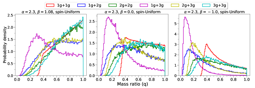
Figure 4: The mass ratio distribution as a function of BBH merger generation. Each panel assumes $\alpha=2.3$ and a uniform spin distribution for 1g BHs, but applies different assumptions about the pairing probability, $\beta=(1.08,0.0,-1.0)$. The mass ratio distribution for higher generation asymmetric mergers peaks at lower values of the mass ratio. Using a beta distribution for the 1g BH spins has a negligible visual impact on these plots. The sampling error on the y-axis values are of order $\sim\mathcal{O}(10^{-2})$, with 90% credibility based on 100 realizations.

References

- Abbott et al. (2019) Abbott, B. P., et al. 2019, Astrophys. J. Lett., 882, L24
- Abbott et al. (2020) Abbott, R., et al. 2020, Phys. Rev. D, 102, 043015
- Abbott et al. (2021a) —. 2021a, arXiv:2111.03606
- Abbott et al. (2021b) —. 2021b, arXiv:2111.03634
- Abbott et al. (2021c) —. 2021c, Astrophys. J. Lett., 913, L7
- Antonini & Gieles (2020) Antonini, F., & Gieles, M. 2020, Mon. Not. Roy. Astron. Soc., 492, 2936
- Antonini et al. (2022) Antonini, F., Gieles, M., Dosopoulou, F., & Chattopadhyay, D. 2022, arXiv:2208.01081
- Antonini et al. (2019) Antonini, F., Gieles, M., & Gualandris, A. 2019, Mon. Not. Roy. Astron. Soc., 486, 5008
- Antonini & Rasio (2016) Antonini, F., & Rasio, F. A. 2016, Astrophys. J., 831, 187
- Arca-Sedda & Gualandris (2018) Arca-Sedda, M., & Gualandris, A. 2018, Mon. Not. R. Astron. Soc., 477, 4423
- Bailyn et al. (1998) Bailyn, C. D., Jain, R. K., Coppi, P., & Orosz, J. A. 1998, Astrophys. J., 499, 367
- Banerjee (2018) Banerjee, S. 2018, Mon. Not. Roy. Astron. Soc., 473, 909
- Barausse et al. (2012) Barausse, E., Morozova, V., & Rezzolla, L. 2012, Astrophys. J., 758, 63, [Erratum: Astrophys.J. 786, 76 (2014)]
- Barausse & Rezzolla (2009) Barausse, E., & Rezzolla, L. 2009, ApJ, 704, L40
- Barkat et al. (1967) Barkat, Z., Rakavy, G., & Sack, N. 1967, Phys. Rev. Lett., 18, 379. https://link.aps.org/doi/10.1103/PhysRevLett.18.379
- Bartos et al. (2017) Bartos, I., Kocsis, B., Haiman, Z., & Márka, S. 2017, Astrophys. J., 835, 165
- Belczynski et al. (2016) Belczynski, K., Holz, D. E., Bulik, T., & O’Shaughnessy, R. 2016, Nature, 534, 512
- Belczynski et al. (2012) Belczynski, K., Wiktorowicz, G., Fryer, C. L., Holz, D. E., & Kalogera, V. 2012, ApJ, 757, 91
- Bellovary et al. (2016) Bellovary, J. M., Mac Low, M.-M., McKernan, B., & Ford, K. E. S. 2016, Astrophys. J. Lett., 819, L17
- Britt et al. (2021) Britt, D., Johanson, B., Wood, L., Miller, M. C., & Michaely, E. 2021, Mon. Not. Roy. Astron. Soc., 505, 3844
- Campanelli et al. (2007) Campanelli, M., Lousto, C. O., Zlochower, Y., & Merritt, D. 2007, Astrophys. J. Lett., 659, L5
- Chattopadhyay et al. (2022) Chattopadhyay, D., Hurley, J., Stevenson, S., & Raidani, A. 2022, Mon. Not. Roy. Astron. Soc., 513, 4527
- de Mink & Mandel (2016) de Mink, S. E., & Mandel, I. 2016, Mon. Not. Roy. Astron. Soc., 460, 3545
- Doctor et al. (2021) Doctor, Z., Farr, B., & Holz, D. E. 2021, Astrophys. J. Lett., 914, L18
- Doctor et al. (2019) Doctor, Z., Wysocki, D., O’Shaughnessy, R., Holz, D. E., & Farr, B. 2019, arXiv:1911.04424
- Dominik et al. (2015) Dominik, M., Berti, E., O’Shaughnessy, R., et al. 2015, Astrophys. J., 806, 263
- Downing et al. (2010) Downing, J. M. B., Benacquista, M. J., Giersz, M., & Spurzem, R. 2010, Mon. Not. Roy. Astron. Soc., 407, 1946
- Farmer et al. (2020) Farmer, R., Renzo, M., de Mink, S., Fishbach, M., & Justham, S. 2020, Astrophys. J. Lett., 902, L36
- Farmer et al. (2019) Farmer, R., Renzo, M., de Mink, S. E., Marchant, P., & Justham, S. 2019, arXiv:1910.12874
- Favata et al. (2004) Favata, M., Hughes, S. A., & Holz, D. E. 2004, Astrophys. J. Lett., 607, L5
- Fishbach & Holz (2020) Fishbach, M., & Holz, D. E. 2020, Astrophys. J. Lett., 891, L27
- Fishbach et al. (2017) Fishbach, M., Holz, D. E., & Farr, B. 2017, Astrophys. J. Lett., 840, L24
- Fitchett (1983) Fitchett, M. J. 1983, Mon. Not. R. Astron. Soc., 203, 1049
- Fowler & Hoyle (1964) Fowler, W. A., & Hoyle, F. 1964, ApJS, 9, 201
- Fragione et al. (2018) Fragione, G., Ginsburg, I., & Kocsis, B. 2018, Astrophys. J., 856, 92
- Fragione & Kocsis (2018) Fragione, G., & Kocsis, B. 2018, Phys. Rev. Lett., 121, 161103
- Fragione & Silk (2020) Fragione, G., & Silk, J. 2020, Mon. Not. Roy. Astron. Soc., 498, 4591
- Georgiev et al. (2016) Georgiev, I. Y., Böker, T., Leigh, N., Lützgendorf, N., & Neumayer, N. 2016, MNRAS, 457, 2122
- Gerosa & Berti (2017) Gerosa, D., & Berti, E. 2017, Phys. Rev. D, 95, 124046
- Gerosa & Berti (2019) —. 2019, Phys. Rev. D, 100, 041301
- Gerosa & Fishbach (2021) Gerosa, D., & Fishbach, M. 2021, Nature Astron., 5, 749
- Gerosa et al. (2021) Gerosa, D., Giacobbo, N., & Vecchio, A. 2021, Astrophys. J., 915, 56
- Gerosa & Kesden (2016) Gerosa, D., & Kesden, M. 2016, Phys. Rev. D, 93, 124066
- Gerosa & Sesana (2015) Gerosa, D., & Sesana, A. 2015, Mon. Not. Roy. Astron. Soc., 446, 38
- Harris (1996) Harris, W. E. 1996, AJ, 112, 1487
- Hofmann et al. (2016) Hofmann, F., Barausse, E., & Rezzolla, L. 2016, Astrophys. J. Lett., 825, L19
- Hurley et al. (2016) Hurley, J. R., Sippel, A. C., Tout, C. A., & Aarseth, S. J. 2016, PASA, 33, e036
- Kimball et al. (2021) Kimball, C., et al. 2021, Astrophys. J. Lett., 915, L35
- Kouwenhoven et al. (2009) Kouwenhoven, M. B. N., Brown, A. G. A., Goodwin, S. P., Zwart, S. F. P., & Kaper, L. 2009, Astron. Astrophys., 493, 979
- Kroupa (2001) Kroupa, P. 2001, Mon. Not. Roy. Astron. Soc., 322, 231
- Li (2022) Li, G.-P. 2022, Phys. Rev. D, 105, 063006
- Lousto & Zlochower (2008) Lousto, C. O., & Zlochower, Y. 2008, Phys. Rev. D, 77, 044028
- Lousto & Zlochower (2013) —. 2013, Phys. Rev. D, 87, 084027
- Lousto et al. (2012) Lousto, C. O., Zlochower, Y., Dotti, M., & Volonteri, M. 2012, Phys. Rev. D, 85, 084015
- Mahapatra et al. (2021) Mahapatra, P., Gupta, A., Favata, M., Arun, K. G., & Sathyaprakash, B. S. 2021, Astrophys. J. Lett., 918, L31
- Mapelli et al. (2021a) Mapelli, M., Santoliquido, F., Bouffanais, Y., et al. 2021a, Symmetry, 13, 1678
- Mapelli et al. (2021b) Mapelli, M., et al. 2021b, Mon. Not. Roy. Astron. Soc., 505, 339
- Marchant et al. (2016) Marchant, P., Langer, N., Podsiadlowski, P., Tauris, T. M., & Moriya, T. J. 2016, Astron. Astrophys., 588, A50
- Marchant et al. (2018) Marchant, P., Renzo, M., Farmer, R., et al. 2018, arXiv:1810.13412
- McKernan et al. (2012) McKernan, B., Ford, K. E. S., Lyra, W., & Perets, H. B. 2012, MNRAS, 425, 460
- McKernan et al. (2018) McKernan, B., Ford, K. E. S., Bellovary, J., et al. 2018, ApJ, 866, 66
- Merritt et al. (2004) Merritt, D., Milosavljević, M., Favata, M., Hughes, S. A., & Holz, D. E. 2004, Astrophys. J, 607, L9
- Miller & Hamilton (2002) Miller, M. C., & Hamilton, D. P. 2002, Mon. Not. Roy. Astron. Soc., 330, 232
- Miller & Lauburg (2009) Miller, M. C., & Lauburg, V. M. 2009, Astrophys. J., 692, 917
- O’Leary et al. (2016) O’Leary, R. M., Meiron, Y., & Kocsis, B. 2016, Astrophys. J. Lett., 824, L12
- Özel et al. (2010) Özel, F., Psaltis, D., Narayan, R., & McClintock, J. E. 2010, ApJ, 725, 1918
- Petrovich & Antonini (2017) Petrovich, C., & Antonini, F. 2017, Astrophys. J., 846, 146
- Pinsonneault & Stanek (2006) Pinsonneault, M. H., & Stanek, K. Z. 2006, Astrophys. J. Lett., 639, L67
- Portegies Zwart & McMillan (2000) Portegies Zwart, S. F., & McMillan, S. 2000, Astrophys. J. Lett., 528, L17
- Renzo et al. (2020) Renzo, M., Farmer, R., Justham, S., et al. 2020, Astron. Astrophys., 640, A56
- Rodriguez et al. (2018) Rodriguez, C. L., Amaro-Seoane, P., Chatterjee, S., et al. 2018, Phys. Rev. D, 98, 123005
- Rodriguez et al. (2016a) Rodriguez, C. L., Chatterjee, S., & Rasio, F. A. 2016a, Phys. Rev. D, 93, 084029
- Rodriguez et al. (2016b) —. 2016b, Phys. Rev. D, 93, 084029. https://link.aps.org/doi/10.1103/PhysRevD.93.084029
- Rodriguez et al. (2015) Rodriguez, C. L., Morscher, M., Pattabiraman, B., et al. 2015, Phys. Rev. Lett., 115, 051101, [Erratum: Phys.Rev.Lett. 116, 029901 (2016)]
- Rodriguez et al. (2020) Rodriguez, C. L., et al. 2020, Astrophys. J. Lett., 896, L10
- Sigurdsson & Hernquist (1993) Sigurdsson, S., & Hernquist, L. 1993, Nature, 364, 423
- Tagawa et al. (2020) Tagawa, H., Haiman, Z., Bartos, I., & Kocsis, B. 2020, Astrophys. J., 899, 26
- Talbot & Thrane (2017) Talbot, C., & Thrane, E. 2017, Phys. Rev. D, 96, 023012
- Talbot & Thrane (2018) —. 2018, Astrophys. J., 856, 173
- Tiwari (2021) Tiwari, V. 2021, Class. Quant. Grav., 38, 155007
- Tiwari (2022) —. 2022, Astrophys. J., 928, 155
- Tiwari & Fairhurst (2021) Tiwari, V., & Fairhurst, S. 2021, Astrophys. J. Lett., 913, L19
- Webb & Leigh (2015) Webb, J. J., & Leigh, N. W. C. 2015, MNRAS, 453, 3278
- Woosley (2016) Woosley, S. E. 2016, Astrophys. J. Lett., 824, L10
- Woosley (2017) —. 2017, Astrophys. J., 836, 244
- Wysocki et al. (2019) Wysocki, D., Lange, J., & O’Shaughnessy, R. 2019, Phys. Rev. D, 100, 043012
- Yang et al. (2019) Yang, Y., Bartos, I., Haiman, Z., et al. 2019, Astrophys. J., 876, 122
- Zevin & Holz (2022) Zevin, M., & Holz, D. E. 2022, arXiv:2205.08549
- Zevin et al. (2019) Zevin, M., Samsing, J., Rodriguez, C., Haster, C.-J., & Ramirez-Ruiz, E. 2019, Astrophys. J., 871, 91