Attention Capture

Abstract

We study the extent to which information can be used to extract attention from a decision maker (DM) for whom waiting is costly, but information is instrumentally valuable. We show all feasible joint distributions over stopping times and actions are implementable by inducing either an extremal stopping belief or a unique continuation belief. For a designer with arbitrary preferences over DM’s stopping times and actions, there is no commitment gap—optimal information structures can always be modified to be sequentially-optimal while preserving the joint distribution over times and actions. Moreover, all designer-optimal structures leave DM with no surplus. We then solve the problem of a designer with arbitrary increasing preferences over DM’s stopping times: optimal structures gradually steer DM’s continuation beliefs toward a basin of uncertainty and have a “block structure”. We further solve the problem of a designer with preferences over both DM’s stopping times and actions for binary states and actions: when the designer’s preferences over times and actions are (i) additively separable, optimal structures take a “bang-bang structure”; (ii) supermodular, optimal structures take a “pure bad news structure”. Our results speak directly to the attention economy.

1  Introduction

The modern age is brimming with information—a vast ocean which exponentially accumulates. Yet, our access to this information is, in practice, mediated by platforms which funnel our attention toward algorithmically curated streams of content—articles to digest, videos to watch, feeds to scroll—which we have little control over. We are inundated with information, yet not truly free to explore the ocean’s depths. These platforms, in turn, generate revenue primarily through advertisements; their business, therefore, is to capture, repackage, and monetize attention.

Motivated by these developments, we study the extent to which information can be used to capture attention. A designer mediates a single decision maker (DM)’s knowledge by choosing some dynamic information structure. The DM values information instrumentally and, at each point in time, chooses between observing more information generated by this dynamic information structure, or stopping and taking action based on her best available information. The designer faces the following trade off: if it gives too much information too quickly, the DM learns what she needs and takes action early; conversely, if it gives the DM too little information, the DM might not find it optimal to keep paying attention—perhaps because waiting is costly, or because she dislikes advertisements—and stops to act even though she is relatively uncertain. Our contribution is to give a relatively complete analysis of (i) joint distributions over stopping times and actions achievable through dynamic information structures; (ii) modifications such that every designer-optimal structure can be made time-consistent; (iii) DM surplus; (iv) designer-optimal structures under arbitrary preferences over DM stopping times; and (v) designer-optimal structures under additively-separable and supermodular preferences over DM actions and stopping times for the case of binary states and actions.

1.1  Outline of contribution

Reduction to extremal and obedient structures. Fix a dynamic information structure which, for each time and each history, specifies a joint distribution over messages and states. This induces some joint distribution over DM’s action and stopping times: on some paths of message realizations, the DM might become confident enough that she stops early and takes action; on other paths, the DM might observe information for a long stretch. Our first result (Proposition 1), and a tool for the rest our analysis, is a reduction principle: for any joint distribution of actions and stopping times achievable by some dynamic information structure, we can achieve the same distribution through a dynamic information structure which (i) induces extremal beliefs at which the DM is either certain of the state, or is indifferent between actions; and (ii) a sequence of unique continuation beliefs (belief paths) at which the DM prefers to continue paying attention—these belief paths play a key role in shaping DM’s continuation incentives, as well as her disposition to take different actions. We call these extremal and obedient dynamic information structures. This holds quite generally, and applies to any decision problem for which DM dislikes delay and nests standard functional forms (e.g., per-period cost, exponential discounting).

Figure 1: Illustration of Propositions 1 and 2

Designer-optimal structures can always be implemented time-consistently. Now consider a designer with with arbitrary preferences over the DM’s action and stopping time. From the reduction principle, optimal structures can always be extremal and obedient. However, such structures often require commitment to future information. Our next result (Proposition 2) states that we can always find sequentially optimal modifications such that at every history, the designer has no incentive to deviate. We show this by showing a tight connection between sequential optimality and DM’s indifference in optimal stopping problems. Every optimal extremal and obedient structure can be modified such that the DM’s continuation belief is no longer necessarily unique, but at each continuation belief, the DM is exactly indifferent between continuing to pay attention and stopping. This, in turn, implies sequential optimality for the designer. The connection between DM indifference and sequential optimality is subtle and the key idea as as follows: DM indifference exactly pins down the DM’s utility at each continuation node as simply the DM’s expected payoff from taking action immediately under her current belief. If any continuation dynamic information structure stemming from any history were not sequentially optimal, the designer could modify the continuation information structure to do strictly better whilst preserving the DM’s continuation incentives at previous histories.

Designer-optimal structures leave DM with no surplus. We next consider the welfare implications of designer-optimal structures when a designer’s payoff is increasing in the DM’s stopping time. If the DM’s preferences are stationary, we show that all designer-optimal structures leave the DM with no surplus i.e., as well-off as if she had acted at time $0$ under her prior. This is so even if the designer and DM’s preferences over actions are aligned, or if the designer’s value for information outstrips the DM’s cost of waiting—the designer is always able to fully extract the DM’s surplus along the attention dimension.

Information structures to extract attention. We then turn to the question of the distributions over stopping times which can be implemented. All feasible stopping times can be implemented by full-revelation and obedient structures in which only certain extremal beliefs—those where the DM is certain of the state—are induced. All feasible stopping time can be implemented by such structures which, in addition, have increasing and extremal belief paths (Proposition 4): the paths are increasing in the sense that conditional on not having learnt the state, the DM’s uncertainty increases over time, and her continuation beliefs are progressively steered towards a region at which her value for information is maximized. As time grows large, the DM’s beliefs also converge to this region. The paths are extremal in the sense that along this path, her beliefs move as much as the martingale constraint on beliefs will allow.

We then detail a class of information structures which solves the designer’s problem for any increasing value and cost function; optimal structures take on a block structure: time is split into blocks of consecutive periods. On the interior of each block, the DM receives no information with probability one; on the boundaries of each block, the DM learns the state with probability which makes her exactly indifferent between paying attention and stopping. This block structure has the natural interpretation as the policy of a platform which controls the duration of advertisements (length of each block). Over the duration of each advertisement (interior of each block), the DM receives no information; at the end of each advertisement (boundary of each block), the designer gives the DM full information with some probability, and shows the DM yet another advertisement with complementary probability. Crucially, since the DM has already sunk her attention costs, conditional on being shown yet another advertisement, she finds it optimal to continue paying attention although she would have been better-off not paying attention in the first place.

We then employ the block structure characterization to solve for designer-optimal structures when their value for attention is nonlinear. When the designer’s value for attention is concave, the optimum can be implemented by giving full information with probability one at a fixed, deterministic time, and no information otherwise. When it is convex, the optimum can be implemented by giving the DM full information at a geometric arrival rate. These structures are two extremes on either end of the space of block structures. When it is ‘S-shaped’ as studied extensively in the marketing literature, the designer’s optimal structure can be implemented through a suitable mixture of the concave and convex optimal structures outlined above.

Information structures to both extract attention and persuade. Finally, we consider the problem of a designer with joint preferences over the DM’s actions and stopping times for the case of binary states and actions. When designer preferences over actions and stopping times are additively separable, designer-optimal structures take a “bang-bang” form in which the designer either focuses on extracting attention, or persuades in one-shot at a fixed, deterministic time. When designer preferences over actions and stopping times are supermodular, designer-optimal structures they take a “pure bad news” form: before some fixed time $T$, the DM stops only upon arrival of conclusive bad news (i.e., learns the state is $0$); conditional on not having stopped before a fixed terminal time $T$, the DM then takes her optimal action under state $1$ (which coincides with the designer-preferred action) at time $T$. The arrival of bad news serves multiple purposes: (i) it generates incentives for the DM to continue paying attention before time $T$; (ii) it pushes the DM’s continuation beliefs up towards state $1$ which, in turn, further increases the value of bad news; and (iii) it maximally delays the DM’s stopping time conditional on taking the designer’s preferred action. Under additional assumptions on the designer’s value function, we show that the designer-optimal structure takes an almost-geoemtric bad news form in which the DM’s continuation beliefs exhibit an initial jump before bad news arrives with constant conditional probability which leads continuation beliefs to drift gradually upwards until the terminal time $T$.

1.2  Related literature

Dynamic information design. Our paper contributes to the burgeoning literature in dynamic information design. Knoepfle (2020) studies competition for attention among multiple designers. The contemporaneous paper of Hébert and Zhong (2022) studies the case in which a designer wishes to maximise the difference of a generalized entropy measure and model the DM as having limited processing capacity which constrains the extent to which beliefs can move between periods. Smolin (2021) and Ely and Szydlowski (2020) study how information can be used to incentivize an agent who decides when to stop exerting effort. Orlov, Skrzypacz, and Zryumov (2020) study how information can be used to influence the exercise time of options. Ely (2017); Ball (2019); Zhao, Mezzetti, Renou, and Tomala (2020) study how information can be used to incentivize effort an agent who makes a choice every period. Che, Kim, and Mierendorff (2023) studies dynamic persuasion when Poisson signals can be generated by the designer and processed by the DM at some cost. Escudé and Sinander (2023) study dynamic persuasion when information can be generated only slowly.

Our contribution is distinct from these papers in several regards. First, the reduction principle we develop makes progress on understand all joint distributions over stopping times and actions which can be achieved through information rather than solving for equilibria in particular contracting settings. Second, we show that designer-optimal information structures can always be modified to be sequentially-optimal and hence time-consistent: this implies that the outcomes (i.e., distributions over action and stopping times) of Markov-perfect equilibria coincides with equilibria in which the designer can commit ex-ante to the full information structure. Indeed, an approach in the literature is to first solve for the optimal structure under commitment, and then verify that it happens to be sequentially optimal (Knoepfle, 2020; Hébert and Zhong, 2022). We show that sequential optimality can always be obtained, no matter the designer or DM’s preferences. Third, we solve the problem of a designer with nonlinear preferences over DM’s stopping times (concave, convex, ‘S-shaped’, arbitrarily increasing). This is in contrast to much of the recent literature which has made progress on the linear case which requires studying only the time-$0$ obedience constraint. Finally, we solve the problem of a designer with joint preferences over both DM’s action and stopping times which, to our knowledge, has not been previously studied.

Information acquisition. Our paper is related to the literature on rational inattention and costly information acquisition (Sims (2003), Pomatto, Strack, and Tamuz (2018), Morris and Strack (2019), Zhong (2022)). In these models, the DM is typically free to choose any information structure but pays a cost which varies with this choice (e.g., increasing in the Blackwell order). Our paper complements this literature by studying the opposite case in which the DM has no control over the information structure she faces, and whose cost of paying attention depends only on time.

Sequential learning. Our paper also contributes to the literature on sequential learning, experimentation, and optimal stopping starting from Wald (1947) and Arrow et al. (1949). One set of papers explore settings in which the DM’s attention is optimally allocated across several exogenous and stationary information sources (Austen-Smith and Martinelli, 2018; Che and Mierendorff, 2019; Gossner, Steiner, and Stewart, 2021; Liang, Mu, and Syrgkanis, 2022). In our setting, the DM only faces a single source of information and our motivation is to understand how distributions of stopping times vary with the information structure. Fudenberg, Strack, and Strzalecki (2018) study the tradeoff between a DM’s speed and accuracy within an uncertain-difference drift-diffusion model driven by Brownian signals. Our reduction principle and results on the joint distributions between actions and stopping times paves the way to more general analyses of speed vs accuracy over all possible information structures.

Direct recommendations and extremal beliefs. The reduction principle explicitly modifies the DM’s beliefs so that (i) her stopping beliefs are extremal; and (ii) her continuation beliefs are unique by collapsing continuation histories. Part (i) is reminiscent of the techniques used in Bergemann, Brooks, and Morris (2015) who, in a static monopoly setting, show that it is sufficient to consider extremal markets. Part (ii) bears resemblance to the classic revelation principle (Gibbard, 1973; Myerson, 1982, 1986). More recently, Ely (2017) develops an ‘obfuscation principle’ which, roughly, states that the designer can simply tell the DM what her beliefs should be after every history. The reduction principle goes a step further by modifying beliefs explicitly.

Information design with nonlinear preferences. Finally, there is recent interest in static persuasion when preferences over DM’s actions are nonlinear (Dworczak and Kolotilin, 2022; Kolotilin, Corrao, and Wolitzky, 2022). We complement this by studying a dynamic setting with nonlinear preferences over stopping times. We employ different tools and, after reducing the nonlinear problem to optimizing over full-revelation and obedient structures, introduce the notion of conditional concavification to exploit the temporal structure of the problem.

1.3  A simple example

To illustrate a few of the key results in our paper, we begin with a simple example. All supporting calculations are in Online Appendix VII.

Example 1.

Part I illustrates how any joint distribution over stopping times and actions can be implemented via extremal and obedient information structures. Part II illustrates how designer-optimal extremal and obedient information structures can always be modified to be sequentially optimal and hence time-consistent. In subsequent sections when we study designer-optimal structures we will continue to build on this example.

Part I: Reduction. There is a single decision maker (DM) whose payoff from choosing action $a\in\{0,1\}$ when the state is $\theta\in\{0,1\}$ at time $t\in\{0,1,2,\ldots\}$ is $-(a-\theta)^{2}-ct$ with $c=1/6$ which is the per-unit-time cost of waiting. DM has prior $\mathbb{P}(\theta=1)=1/3$ and faces a dynamic information structure which, for each state, time, and history of past messages, specifies a distribution over messages.

Figure 2: Reduction to extremal and obedient structures

The left panel of Figure 2 illustrates an arbitrary information structure $I$. The numbers in the nodes represent the DM’s beliefs at that node, and the numbers on the branches stemming from each node represent the transition probabilities of DM’s beliefs conditional on being at that node. It is straightforward to verify that for $c=1/6$, the nodes at which the DM stops (marked in red) are in fact optimal.

First consider the following modification: on the nodes at which the DM stops in the original information structure $I$, we instead extremize the DM’s beliefs. More explicitly, the DM’s optimal action is $1$ for the beliefs $[1/2,1]$, and optimal action is $0$ for the beliefs $[0,1/2]$. Taking the union of the extreme points of these sets, the DM’s extremal beliefs are $\{0,1/2,1\}$. Now suppose that DM stops at belief $5/6$ on the original structure $I$. We then modify the structure to instead have DM stop at extreme belief $1$ with probability $2/3$, and extreme belief $1/2$ with probability $1/3$—we represent this modification with the single node ‘Ext’. By extremizing every stopping node, we obtain the information structure $I^{\prime}$ shown in the middle panel of Figure 2. Note that doing so preserves the $DM$’s action which leaves the DM’s payoffs—and hence continuation incentives at non-stopping nodes—unchanged.

Next consider the further modification constructed by taking the information structure $I^{\prime}$ and collapsing the histories at which the DM has belief $1/3$ at $t=1$, and $2/3$ at $t=1$ into a single history at which the DM has belief $1/2$ at time $t=1$. This modification is depicted by the information structure $I^{\prime\prime}$ on the right panel of Figure 2. A key observation is that the DM’s beliefs at the collapsed history ($5/18$) is a mean-preserving contraction of her beliefs at the original histories ($1/2$ and $1/3$). By the convexity of the max operator and Jensen’s inequality, this implies that if she did find it optimal to continue at the original histories, she must also find it optimal to continue at the collapsed history. We have thus obtained the information structure $I^{\prime\prime}$ which is extremal in the sense that all stopping beliefs are in the set $\{0,1/2,1\}$, and obedient in the sense that continuation beliefs are unique. This information structure preserves the joint distribution over the DM’s actions and stopping times. Proposition 1 extends this logic to many states and actions, and arbitrary decision problems and delay costs.

Part II: Time-Consistent Modifications.Now suppose that if the DM stops at time $\tau$ and takes action $a$, the designer’s payoff is $f(\tau,a)$. The designer thus has preferences over the DM’s actions and stopping time. Now suppose, for this example, that $f(\tau,a)=\log(\tau)$ so the designer only wishes to extract attention, and has concave preferences over the DM’s stopping time. We claim that the unique distribution of stopping beliefs puts probability $1$ on $\tau=3$ to deliver a payoff of $\log 3$. As we previously saw, this can always be implemented through extremal and obedient structures by giving the DM no information with probability $1$ at time $1$, and then full information with probability $1$ at time $2$. This is illustrated by the extremal and obedient information structure on the left of Figure 3.

Figure 3: Modification to be time-consistent

Note, however, that the implementation of this dynamic information structure requires commitment to future information: the DM has to trust that at all histories, the designer will follow through with their promise and give the DM full information about the state in the next period. However, we see that at time $t=2$, the designer has an incentive to deviate: since the DM has already sunk her attention costs, it is no longer sequentially optimal for the designer to follow-through with their promise.

Now consider the modification depicted in Figure 3 in which instead of inducing the unique beliefs $1/3$ at time $t=1$, the designer instead induced the beliefs $7/9$ and $2/9$. At time $t=2$, the designer induces the belief $8/9$ and $1/9$. Finally, at $t=3$, the designer gives the DM full information which we represent with “Full”. Observe that this corresponds to DM indifference at every continuation node. For instance, at the node $8/9$, the DM is indifferent between stopping at time $t=2$ and taking action $1$, yielding an expected payoff of $-1/9$, or paying an extra cost of $c=1/9$ to learn the state at time $t=3$. If the DM is indifferent at every continuation node, this then implies that the information structure must be sequentially-optimal for the designer, and hence time-consistent. Proposition 2 shows that this holds more generally with many states and actions, for arbitrary designer preferences over actions and stopping times, and arbitrary DM decision problems and delay costs. $\hfill\blacksquare$

The rest of the paper is organized as follows. In Section 2 we develop the general model as well as key definitions. Section 3 develops the reduction principle, shows that optimal time-consistent implementations always exist, and shows designer-optimal designs leave DM with zero surplus. In Section 4 we solve for designer-optimal designs when the designer has increasing preference over DM stopping times. In Section 5 we solve for designer-optimal designs when the designer has preferences over both stopping times and actions. Section 6 concludes.

2  Model

Time is discrete and infinite, indexed by $\mathcal{T}=0,1,2\ldots$. The state space $\Theta$ is finite and state $\theta\in\Theta$ is drawn from the common full-support prior $\mu_{0}\in\Delta(\Theta)$.

2.1  Dynamic information structures

A dynamic information structure specifies, for each time $t$ and history of beliefs, a distribution over the next period’s beliefs subject to a martingale constraint as well as a set of messages $M$. We augment the belief-based representations of dynamic information with messages because for the optimal-stopping problems we consider, beliefs alone are insufficient to describe the space of information structures—the same history of beliefs might correspond to different continuation structures which, in turn, correspond to different incentives.

Let $I\in\Delta\big{(}\prod_{t\geq 1}(\Delta(\Theta)\times M)\big{)}$ be a distribution over beliefs and messages. Let the random variable $(\mu_{t},m_{t})_{t}$ be the stochastic path of belief-message pairs associated with $I$, and define $H_{t}:=(\mu_{s},m_{s})_{s\leq t}$ as a time-$t$ history. Define the conditional distribution over next period’s belief-message pairs as follows:

$$I_{t+1}(B|H_{t}):=\int_{\begin{subarray}{c}(\mu_{s},m_{s})_{s>t}:\\ (\mu_{t+1},m_{t+1})\in B\end{subarray}}dI(\cdot|H_{t})\quad\text{for every Borel set $B\in\mathcal{B}(\Delta(\Theta)\times M)$}$$

where $I(\cdot|H_{t})$ is a conditional probability measure under the natural filtration $\mathcal{F}_{t}$ with realization $H_{t}\in\mathcal{F}_{t}$. We say the history $H_{t}$ realizes with positive probability if $\{(\mu_{s},m_{s})_{s}:(\mu_{s},m_{s})_{s\leq t}=H_{t}\}\subset\text{supp}(I)$ i.e., if paths with the first $t$ periods agrees with $H_{t}$ is contained in the support of $I$.

A dynamic information structure $I$ is such that for any time $t\geq 0$ and history $H_{t}$ which realizes with positive probability, the following martingale condition on beliefs holds:

$$\mu_{t}=\int_{\mu_{t+1}\in\Delta(\Theta),m_{t+1}\in M}\mu_{t+1}dI_{t+1}\Big{(}(\mu_{t+1},m_{t+1})|H_{t}\Big{)}.$$

2.2  Decision maker’s payoffs

A single decision maker (DM) faces a decision problem. Her payoff from taking action $a$ under state $\theta$ at time $t$ is $v:A\times\Theta\times\mathcal{T}\to\mathbb{R}$ where we impose

$$t>t^{\prime}\implies v(a,\theta,t)<v(a,\theta,t^{\prime}).$$

Impatience simply states that all else equal, the DM would rather act sooner rather than later. It nests (i) per-period costs: $v(a,\theta,t)=u(a,\theta)-c\cdot t$; and (ii) exponential discounting: $v(a,\theta,t)=\delta^{t}u(a,\theta)$ for strictly positive $u$.

2.3  Measures under different dynamic information structures

We will often vary the dynamic information structure to understand how variables of interest (e.g., probabilities of histories, incentive compatibility constraints etc.) change. To this end, we will use $\mathbb{E}^{I}[\cdot]$, $\mathbb{E}^{I}[\cdot|\cdot]$, $\mathbb{P}^{I}(\cdot)$, and $\mathbb{P}^{I}(\cdot|\cdot)$ to denote the unconditional and conditional expectations and probabilities under dynamic information structure $I\in\mathcal{I}$. Throughout this paper we use superscripts to track dynamic information structures, and subscripts to track time periods.

2.4  Decision maker’s problem

Facing a dynamic information structure $I\in\mathcal{I}$, the DM solves the following optimization problem:

$$\sup_{\tau,a_{\tau}}\mathbb{E}^{I}[v(a_{\tau},\theta,\tau)],$$

where $\tau$ is a stopping time and $a_{\tau}$ is a (stochastic) action under the natural filtration.Throughout we will assume that the DM breaks indifferences in favour of not stopping. This will ensure that the set of feasible stopping times is closed though it is not essential for the main economic insights.

2.5  Feasible joint distributions of actions and stopping times

For a given information structure $I\in\mathcal{I}$, this induces the DM to stop at random times and take random actions. Define $d(I)\in\Delta(A\times\mathcal{T})$ as the joint distribution induced by $I$. Define the pair of random variables $(a_{\tau(I)},\tau(I))\sim d(I)$ as the action and the stopping time associated with $I$ where we drop dependence on $I$ when there is no ambiguity.

Definition 1 (Feasible distributions).

The joint distribution $d\in\Delta(A\times\mathcal{T})$ is feasible if there exists an information structure $I\in\mathcal{I}$ such that $d=d(I)$. The marginal distribution over stopping times $d_{\mathcal{T}}\in\Delta(\mathcal{T})$ is feasible if there exists $I\in\mathcal{I}$ such that $\text{marg}_{\mathcal{T}}d(I)=d_{\mathcal{T}}$.

2.6  Extremal and obedient dynamic information structures

We now introduce a special class of information structures which will play a crucial role in much of our analysis.

Define $v_{t}^{*}(\mu):=\max_{a\in A}\mathbb{E}_{\theta\sim\mu}v(a,\theta,t)$ and $a^{*}_{t}(\mu):=\text{argmax}_{a\in A}\mathbb{E}_{\theta\sim\mu}v(a,\theta,t)$ as the DM’s time-$t$ indirect utility and best-response correspondence respectively. For the subset of actions $A^{\prime}\subseteq A$, define

$$X_{A^{\prime},t}:=\Big{\{}\mu\in\Delta(\Theta):A^{\prime}\subseteq a^{*}_{t}(\mu)\Big{\}}\quad X^{EXT}_{{A^{\prime},t}}:=\text{Ext}(X_{A^{\prime}})$$

as the set of beliefs for which actions in $A^{\prime}$ are optimal, and the extreme points of that set respectively. Call $X^{EXT}_{t}:=\bigcup_{A^{\prime}\subseteq A}X^{EXT}_{A^{\prime},t}$ the set of time-$t$ extremal stopping beliefs. Observe that the degenerate beliefs at which DM is certain the state is also extremal.

For Example 1 in the introduction we had additively separable delay costs so $X^{EXT}_{t}$ was constant over time: for all $t$,

$$\begin{rcases*}X_{\{0\},t}=[0,1/2]&$\implies X^{EXT}_{\{0\},t}=\{0,1/2\}$\\ X_{\{1\},t}=[1/2,1]&$\implies X^{EXT}_{\{1\},t}=\{1/2,1\}$\\ X_{\{0,1\},t}=\{1/2\}&$\implies X^{EXT}_{\{0,1\},t}=\{1/2\}$\end{rcases*}\implies X^{EXT}_{t}=\bigcup_{A^{\prime}\subseteq\{0,1\}}X_{A^{\prime},t}=\{0,1/2,1\}$$

Definition 2 (Extremal and obedient).

$I$ is extremal and obedient if $M=\{C,S\}$ and there exists a unique continuation belief path $(\mu^{C}_{t})_{t}$ such that for any $H_{t}$ which realizes with positive probability,

1. (Extremal stopping beliefs and unique continuation beliefs) the support of time $t+1$ beliefs associated with message $S$ are contained within the set of extremal beliefs and time $t+1$ beliefs associated with the message $C$ follow the belief path:

   $$\text{supp}\,I\big{(}(\cdot,S)|H_{t}\big{)}\subseteq X^{EXT}_{t+1}\quad\text{supp}\,I\big{(}(\cdot,C)|H_{t}\big{)}\subseteq\{\mu^{C}_{t+1}\};$$

2. (Obedience) for any $(\mu_{t+1},m)$ pair with realizes with positive probability from $H_{t}$, DM prefers to stop at $(\mu_{t+1},S)$ and continue at $(\mu_{t+1},C)$.

Call the set of extremal and obedient structures $\mathcal{I}^{EXT}$.

Figure 4: Illustration of extremal and full-revelation structures

Extremal and obedient structures are such that the DM’s stopping beliefs at time $t+1$ always lie in the set of extremal beliefs $X^{EXT}_{t+1}$ and her continuation belief is unique: conditional on waiting up to time $t+1$, her beliefs at $t+1$ is pinned down as $\mu^{C}_{t+1}$. They are depicted on the left in Figure 4 for the DM’s preferences in Example 1

We will sometimes be concerned only with the distribution of stopping times—it is then sufficient to consider a smaller class of information structures at which the DM stops only when she is certain of the state. Such structures are depicted on the right in Figure 4 for the DM’s preferences in Example 1.

Definition 3.

(Full-revelation and obedient) $I$ is full-revelation and obedient if it is extremal and obedient, and in addition for any $H_{t}$ which realizes with positive probability,

$$\text{supp}\,I\big{(}(\cdot,S)|H_{t}\big{)}\subseteq X^{FULL}:=\{\delta_{\theta}:\theta\in\Theta\}.$$

Call the set of full-revelation and obedient information structures $\mathcal{I}^{FULL}$.

2.7  Designer’s problem

Suppose there is a designer with preferences $f:A\times\mathcal{T}\to\mathbb{R}$. The designer’s problem is under full commitment (i.e., if they could commit to future information structures) is

$$\sup_{I\in\mathcal{I}}\mathbb{E}^{I}[f(a_{\tau},\tau)].$$

noting that the supremum is taken over the whole space of feasible dynamic information structures. We will assume enough regularity assumptions so that the set of feasbile joint distributions is closed hence the supremum is obtained.

Definition 4.

$I$ is sequentially optimal for $f$ if for every $H_{t}$ which realizes with positive probability

$$\sup_{I^{\prime}\in\mathcal{I}|H_{t}}\mathbb{E}^{I^{\prime}}[f(a_{\tau},\tau)|H_{t}]=\mathbb{E}^{I}[f(a_{\tau},\tau)|H_{t}]$$

where $\mathcal{I}|H_{t}$ is the set of dynamic information structures where $H_{t}$ realizes with positive probability. Call the set of sequentially-optimal structures $\mathcal{I}^{SEQ}(f)$.

Sequential optimality guarantees that at any history, the designer has no incentive to deviate and pick an alternative information structure—it thus implies time-consistency. Clearly, the designer’s value under full commitment is weakly higher than if she were constrained to be time-consistent:

$$\sup_{I\in\mathcal{I}}\mathbb{E}^{I}[f(a_{\tau},\tau)]\geq\sup_{I^{\prime}\in\mathcal{I}^{SEQ}(f)}\mathbb{E}^{I^{\prime}}[f(a_{\tau},\tau)].$$

We will show that for any designer preference $f$ and DM preference, this is in fact an equality and give an explicit modification for full-commitment structures to also be time-consistent. Anticipating these results, when we explicitly solve for optimal dynamic information structures in Sections 4 and 5, we will not make a distinction between the full-commitment and no-commitment cases.

3  Reduction and time-consistency for general stopping problems

Out first result shows that it is sufficient to restrict our attention to extremal and obedient structures.

Proposition 1 (Reduction principle).

For any:

1. feasible joint distribution over stopping times and actions $d\in\Delta(A\times\mathcal{T})$, there exists a extremal and obedient structure $I\in\mathcal{I}^{EXT}$ such that $d(I)=d$;

2. feasible marginal distribution over stopping times $d_{\mathcal{T}}\in\Delta(\mathcal{T})$, there exists a full-revelation and obedient structure $I\in\mathcal{I}^{FULL}$ such that $\text{marg}_{\mathcal{T}}d(I)=d_{\mathcal{T}}$.

Part (i) of Proposition 1 states that every feasible distribution $d$ which is achievable by some dynamic information structure is also achievable by extremal and obedient structures. As such, restricting our attention to the set $\mathcal{I}^{EXT}$ is sufficient.

The argument for part (i) of Proposition 1 proceeds in two steps. Fix an arbitrary information structure $I\in\mathcal{I}$. The first step collapses the tree of non-stopping histories together. The key observation here is that when we collapse several time-$t$ histories—say, $H_{t}^{1},H_{t}^{2},\ldots,H_{t}^{n}$—together into the history $H_{t}^{*}$, if the DM did not find it optimal to stop at the histories $H_{t}^{1},H_{t}^{2},\ldots H_{t}^{n}$, then she cannot find it optimal to stop at the collapsed history $H_{t}^{*}$. To see this, first observe that on each history, the DM’s incentives to stop depends on her expected payoff from taking her best action under the current belief at that history. Furthermore, note that the maximum operator is convex. Finally, note that the beliefs on the collapsed history $H_{t}^{*}$, $\mu|H_{t}^{*}$ must be a mean-preserving contraction of the DM’s original beliefs on each of the branches $\mu|H_{t}^{1},\ldots\mu|H_{t}^{n}$. An elementary application of Jensen’s inequality then implies that the DM must do weakly worse by stopping with belief $\mu|H_{t}^{*}$ than a hypothetical lottery over stopping with beliefs $\mu|H_{t}^{1},\mu|H_{t}^{2},\ldots,\mu|H_{t}^{n}$ with mean $\mu|H_{t}^{*}$. As such, if the DM found it optimal to continue paying attention at time $t$ on each of the original histories, she must also find it optimal to do so at the collapsed history. The second step then extremizes the DM’s stopping nodes such that they are supported only on extremal beliefs. Since this does not change the DM’s optimal action at each node, this preserves all prior continuation incentives as well as the joint distribution of stopping times and actions. Part (ii) of Proposition 1 follows straightforwardly from part (i) by noting that if we are only interested in the marginal distribution over stopping times, then it is without loss to give the DM full information whenever she stops—doing so must weakly improve continuation incentives at continuation nodes.

An attractive property of extremal/full-revelation and obedient structures is that continuation histories do not branch—conditional on paying attention up to $t$, there is a unique continuation history and hence continuation belief. This substantially prunes the space of dynamic information structures and will allow us to explicitly solve designer-optimal structures in Sections 4 and 5.

Note, however, that many extremal and obedient structure are not sequentially optimal. For instance, recall Part II of Example 1 in which the structure was extremal and obedient (give the DM full information at $t=3$, and no information before that; depicted in Figure 3) but not sequentially optimal. At time $t=2$, the continuation information structure (give the DM full information in the next period) is sub-optimal since the DM has already sunk her attention costs—the designer can thus do better by delaying the arrival of information. This raises the question of what kinds of joint distributions over times and actions can be implemented when the designer is unable to commit to delivering future information. Our next result states that there is, in general, no commitment gap: for any designer’s value function $f$, there always exists a designer-optimal structure under full commitment $I^{*}\in\mathcal{I}$ we can modify to be sequentially optimal yet induces the same joint distribution over actions and times, and hence achieves the same payoff for the designer.

Proposition 2.

(Sequentially-optimal modifications) For any designer’s preference $f:A\times\mathcal{T}\to\mathbb{R}$, there exists an optimal information structure $I^{*}\in\text{argmax}_{I\in\mathcal{I}}\mathbb{E}[f(a_{\tau},\tau)]$ and a sequentially optimal structure $I^{**}\in\mathcal{I}^{SEQ}(f)$ such that $d(I^{*})=d(I^{**})$. In particular, this implies no commitment gap:

$$\max_{I\in\mathcal{I}}\mathbb{E}^{I}[f(a_{\tau},\tau)]=\max_{I^{\prime}\in\mathcal{I}^{SEQ}(f)}\mathbb{E}^{I^{\prime}}[f(a_{\tau},\tau)].$$

The key intuition underlying Proposition 2 is the tight connection we develop between DM’s indifference and sequential optimality: suppose that structure $I$ is such that for all times $t$ and any positive probability continuation history $H_{t}$, the DM is indifferent between taking action and continuing. Then if $I$ is designer-optimal, it must also be sequentially optimal.

Figure 5: Illustration of connection between indifference and sequential optimality

To see this, suppose that the information structure is optimal but not sequentially optimal from $H_{t}$—this implies that the designer can do better by replacing $I|H_{t}$ with some alternative continuation structure $I^{\prime}|H_{t}$—this modification is depicted in Figure 5 in which the original information structure is on the left, and the modification replacing $I|H_{t}$ (red) with $I^{\prime}|H_{t}$ (blue) is on the right. Note that this modification weakly increases the DM’s continuation incentives at all histories before $H_{t}$. This is because since she was indifferent at $H_{t}$ under $I$, her payoff was from $I|H_{t}$ achieved the lower bound on DM’s continuation incentives which is simply the expected value of acting under belief $\mu_{t}|H_{t}$. Any modification $I^{\prime}|H_{t}$ must therefore weakly increase the DM’s continuation incentives at $H_{t}$ and all earlier histories. Finally, since $H_{t}$ realizes with positive probability and $I^{\prime}|H_{t}$ is strictly preferred by the DM to $I|H_{t}$, this modification strictly improves the DM’s expected payoff which contradicts the optimality of the original structure $I$.

The remaining challenge is to show that all designer-optimal information structures can be made so that the DM is indifferent at every history. The proof is technical and deferred to Appendix B. Here we offer the intuition for the case in which the designer-optimal information structure $I$ induces a bounded stopping time i.e., there exists $T<+\infty$ such that $\mathbb{P}(\tau(I)>T)=0$. First consider the set of (positive probability) continuation histories at time $T-1$ and observe that if there is some history $H_{t-1}$ at which the DM strictly prefers to continue, we can find a new set of histories $(H_{T-1}^{i})_{i=1}^{n}$ such that (i) beliefs at these new histories $(\mu_{t-1}|H^{i}_{T-1})_{i=1}^{n}$ are a mean-preserving spread of the belief $\mu_{T-1}|H_{T-1}$ at the original history; (ii) the DM is indifferent between stopping and continuing at each history $(H_{T-1}^{i})_{i=1}^{n}$; and (iii) the distribution of stopping times and actions stemming from $H_{T-1}$ is preserved over the histories $(H_{T-1})_{i=1}^{n}$. We then recursively modify continuation histories this way to arrive at an information structure which (i) preserves the distribution over actions and stopping times; (ii) preserves DM continuation incentives at each continuation node; and (iii) makes the DM indifferent at each continuation history which, by the argument above, guarantees sequential optimality.

In light of Propositions 1 and 2, in the next section when we explicitly characterize designer-optimal information structures it will be without loss to study extremal (or full-revelation) and unique-continuation structures: by Proposition 1, these structures achieve all feasible joint distributions; by Proposition 2, these structures can always be made time-consistent by suitably modifying continuation beliefs to be non-unique.

3.1  Designer-optimal structures generate no DM surplus

For the remaining results in this paper, we will impose an additional assumption that delay costs are constant per unit time. This assumption has also been adopted by a number of papers on optimal stopping in economics (Fudenberg, Strack, and Strzalecki, 2018; Che and Mierendorff, 2019; Che, Kim, and Mierendorff, 2023). Our results extend fairly readily to the case in which costs are additive but nonlinear.

Assumption (Additively separable cost).

Say that costs are additively separable if we can write

$$v(a,\theta,t)=u(a,\theta)-ct$$

for some constant per-period cost $c>0$ and utility $u:A\times\Theta\to\mathbb{R}$.

Additively separability adds structure to the problem by separating the DM’s value for information from the expected additional cost from waiting.

We now show that for arbitrary decision problem and arbitrary designer preference over stopping actions and times , the DM’s surplus is zero. This implies that even if there are substantial gains from trade e.g., the designer values the DM’s attention more than the DM’s cost of delay, or the designer and DM’s interests are aligned, designer-optimal structures always leave the DM as worse off as if she had not paid any attention and simply took action under her prior.

Proposition 3.

Suppose the designer’s value $f(a,\tau)$ is strictly increasing in $\tau$. For any designer-optimal structure $I^{*}\in\text{argmax}_{I\in\mathcal{I}}\mathbb{E}^{I}[f(a_{\tau},\tau)]$,

$$\max_{a_{\tau},\tau}\mathbb{E}^{I^{*}}[v(a_{\tau},\theta,\tau)]=0.$$

Proposition 3 is proven in Appendix B and proceeds by noting that if DM’s surplus is strictly positive, then the designer can perturb the information structure so that it is delayed with small probability—for a small enough perturbation, this remains obedient for the DM but the designer is strictly better off.

4  Optimal Structures for Attention Capture

We now put the reduction principle to work by deriving general properties on the continuation belief paths of full-revelation and obedient information structures which implement all feasible stopping times. This is of particular interest when the designer only cares about attention i.e., $f(a,t)=h(t)$ for some increasing function $h$. We will then solve for designer-optimal structures under (i) arbitrary $h$; (ii) convex $h$; (iii) concave $h$; (iv) ‘S-shaped’ $h$.

4.1  General properties of structures for all feasible stopping times

Our first goal will be to derive general properties of information structures which implement all feasible stopping times. From Proposition 1 part (ii), we know that it is without loss to consider full-revelation and obedient information structures. The DM’s incentives to continue paying attention at time $t\in\mathcal{T}$ after history $H_{t}$ under information structure $I\in\mathcal{I}^{*}$ is given by the condition

$$\max_{a\in A}\mathbb{E}^{I}[v(a,\theta,t)|H_{t}]\leq\mathbb{E}^{I}[v^{*}_{\tau}(\delta_{\theta})|\tau>t]$$

where $\delta_{\theta}$ is the belief which puts probability $1$ on state $\theta$. There are two sources of uncertainty within the expectation operator on the right: uncertainty over the time at which the DM optimally stops to take action, as well as the payoff the DM will receive then, which depends on what the true state is. When $v(a,\theta,t)$ is an arbitrary function, these two sources of uncertainty can interact in complicated ways. Our additional assumption of additive separability allows us to rewrite the above condition as

$$\underbrace{\mathbb{E}^{I}\Big{[}u^{*}(\theta)|H_{t}\Big{]}-\max_{a\in A}\mathbb{E}^{I}\Big{[}u(a,\theta)|H_{t}\Big{]}}_{\eqqcolon\phi(\mu|H_{t})}\geq\mathbb{E}^{I}\Big{[}c\tau|\tau>t\Big{]}-ct$$

where $u^{*}(\theta):=\max_{a\in A}u(a,\theta)$. Define the map $\phi:\Delta(\Theta)\to\mathbb{R}_{\geq 0}$ such that for all $\mu\in\Delta(\Theta)$,

$$\phi(\mu):=\mathbb{E}_{\mu}[u^{*}(\theta)]-\max_{a\in A}\mathbb{E}_{\mu}[u(a,\theta)].$$

$\phi(\mu)$ is the additional value the DM gains from full information under the belief $\mu$. $\phi$ is continuous and concave since $\mathbb{E}_{\mu}[u^{*}(\theta)]$ is linear and $\max_{a\in A}\mathbb{E}_{\mu}[u(a,\theta)]$ is convex. Define:

$$\Phi^{*}:=\text{argmax}_{\mu\in\Delta(\Theta)}\phi(\mu)\subseteq\Delta(\Theta)\quad\phi^{*}:=\max_{\mu\in\Delta(\Theta)}\phi(\mu).$$

$\Phi^{*}$ is the set of beliefs for which the DM’s benefit from obtaining full information relative to stopping immediately is maximized; $\phi^{*}$ is the maximum of $\phi$. Since $\phi$ is concave, $\Phi^{*}$ is convex. We will often refer to $\Phi^{*}$ as the basin of uncertainty.

Full-revelation and obedient structures can be thought of as choosing both a stopping time $\tau$ with distribution in $\Delta(\mathcal{T})$, as well as a belief path $(\mu_{t})_{t\in\mathcal{T}}$. These two objects impose constraints on each other and are interlinked in the following sense. Fixing a particular belief path $(\mu_{t})_{t}$, whether the stopping time is feasible depends on whether, at each belief $\mu_{t}$, facing the distribution of stopping times going forward, the DM prefers to continue paying attention. We call this the obedience constraint. Furthermore, fixing a particular distribution of stopping times, not every path of beliefs will be compatible—there are paths which violate the martingale requirement. Call this the boundary constraint.

It turns out that the obedience and boundary constraints offer a characterization of feasible stopping times in terms of whether we can find a support belief paths. We formalize this in the following lemma which is proved in Appendix C.

Lemma 1.

The following are equivalent:

1. There exists a full-revelation and obedient information structure $I\in\mathcal{I}^{FULL}$ which induces stopping time $\tau(I)$ and belief path $(\mu_{t}^{C})_{t\in\mathcal{T}}\in(\Delta(\Theta))^{\mathcal{T}}$.

2. The following conditions are fulfilled:

   1. (Obedience constraint) $\phi(\mu_{t}^{C})\geq\mathbb{E}[c\tau\mid\tau>t]-ct$ for every $t\in\mathcal{T}$; and

   2. (Boundary constraint) $\mathbb{P}^{I}(\tau>t+1)\mu_{t+1}^{C}(\theta)\leq\mathbb{P}^{I}(\tau>t)\mu_{t}^{C}(\theta)$ for every $t\in\mathcal{T}$ and $\theta\in\Theta.$

Condition (i) is the usual constraint that at each time $t$, the DM must find it optimal to continue paying attention. Condition (ii) imposes a contraint on the degree to which beliefs can move between periods in terms of the probability that the DM learns the state at time $t+1$ conditional upon paying attention up to time $t$. For instance, if the stopping time is such that the DM never learns the state at time $t+1$, then she does not receive any information between times $t$ and $t+1$ so $\mu_{t}^{C}=\mu_{t+1}^{C}$. We emphasise that this boundary constraint is not an artefact of working in discrete time and would still obtain in continuous time while working on the on the space of right-continuous left-limit belief martingales.

Our next result employs Lemma 1 to develop general properties of belief paths which accompany any feasible stopping time.

Proposition 4.

Every feasible distribution $d_{\tau}\in\{\text{marg}_{\mathcal{T}}d:d\in\mathcal{D}\}$ is induced by a full-revelation and obedient information structure $I\in\mathcal{I}^{FULL}$ with belief path $(\mu_{t}^{C})_{t}$ for which

1. (Increasing paths) $\phi(\mu_{t}^{C})$ is increasing in $t$; and

2. (Extremal paths) for every $t\in\mathcal{T}$, either $\mu_{t+1}\in\Phi^{*}$ or $\frac{\mathbb{P}(\tau>t+1)}{\mathbb{P}(\tau>t)}=\min_{\theta\in\Theta}\frac{\mu_{t}^{C}(\theta)}{\mu_{t+1}^{C}(\theta)}$.

Figure 6: Illustration of increasing and extremal paths

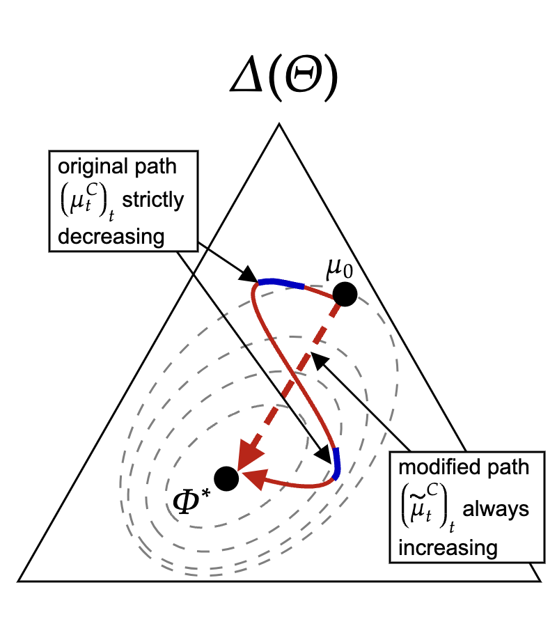
(a) Increasing belief paths

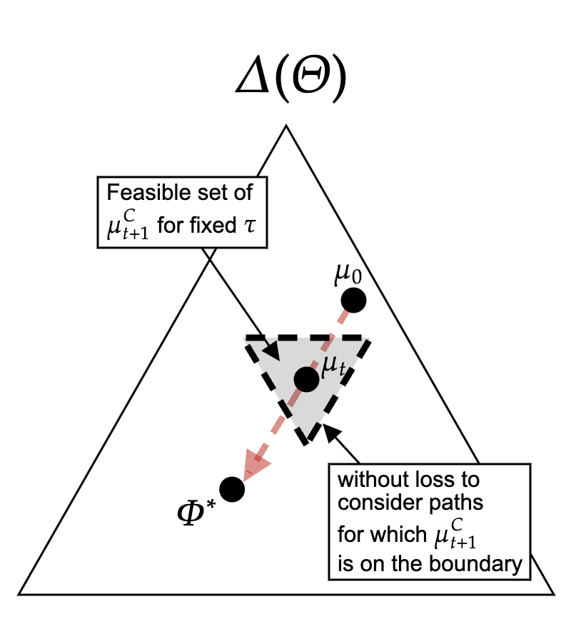
(b) Extremal belief paths

Part (i) states that it is without loss to consider belief paths which are increasing in $\phi$ i.e., the longer the DM goes without learning the state, the more uncertain she is. The underlying intuition is that by steering the DM’s belief toward $\Phi^{*}$, this increases the value of full information for the DM which slackens future obedience constraints. However, the boundary constraint complicates this by imposing a limit on the degree to which beliefs can move between periods. Nonetheless, we can implement any feasible stopping time through increasing paths. This is illustrated in Figure 6b (a) in which the dotted lines are contour lines of $\phi$ (beliefs on the same dotted line have the same value of $\phi$). Starting from an initial belief path $(\mu_{t}^{C})_{t}$ depicted by the solid red line, this might be strictly decreasing in $\phi$ for some times, as depicted by the blue portions. It turns out that we can always find an alternate sequence of beliefs $(\tilde{\mu}^{C}_{t})_{t}$ which still fulfils the obedience and boundary constraints, but which is now increasing in $\phi$. The new sequence of beliefs is illustrated by the dotted red line. Part (ii) states that it is without loss to consider extremal belief paths—those for which before reaching the basin $\Phi^{*}$, the boundary constraint binds. This is illustrated in Figure 6b (b). For belief $\mu_{t}^{C}$ at time $t$, the shaded triangle shows the set of feasible beliefs $\mu_{t+1}^{C}$. Part (ii) states that it is without loss to consider paths for which $\mu_{t+1}^{C}$ is on the boundary of this set, depicted by the black dotted line.

The proof of Proposition 4 is technical and we defer it to Appendix C. Starting from an arbitrary feasible distribution $d_{\tau}\in\Delta(\mathcal{T})$, by the reduction in Proposition 1 part (ii) it is without loss to consider a full-revelation and obedient structure with implements $d_{\mathcal{T}}$. This structure is associated with some belief path $(\mu_{t}^{C})_{t}$—the key challenge is to ‘iron’ this path in a way that (i) preserves obedience at every time $t\in\mathcal{T}$; while (ii) the modified belief path is both increasing in $\phi$ and extremal.

4.2  Designer-optimal under concave value function

We now turn to the simplest case in which the designer’s value function is concave. This nests the case in which the designer’s value function is linear, variants of which are studied by Knoepfle (2020) and Hébert and Zhong (2022).

Proposition 5 (Designer-optimal when $h$ is concave).

Suppose the designer’s value function is concave i.e., $f$ is concave. If $\frac{\phi(\mu_{0})}{c}$ is an integer, then a designer’s optimal information structure is attained by giving full information with full probability at time $\frac{\phi(\mu_{0})}{c}$.

Proof of Proposition 5.

Considering the DM’s incentives at time $0$, we have the following necessary condition for $\tau$ to be strictly positive: $\mathbb{E}^{I}[\tau]\leq\frac{\phi(\mu_{0})}{c}$. Thus, the designer’s utility is bounded above by

$$\mathbb{E}^{I}[h(\tau)]\leq h(\mathbb{E}^{I}[\tau])\leq h\Big{(}\frac{\phi(\mu_{0})}{c}\Big{)},$$

where the first inequality is from Jensen. It is easy to check that the equality holds the information structure that gives full information with full probability at time $\frac{\phi(\mu_{0})}{c}$.∎

Note that the requirement that $\frac{\phi(\mu_{0})}{c}$ is an integer arises because of the discreteness of time in our setting. If it were not an integer, the qualitative properties of designer-information would remain the same, but the DM would instead stop either at time $T$ or $T+1$ where the probabilities are chosen such as to bind her time-$0$ obedience constraint.

The proof of Proposition 5 relied on showing that the time-$0$ obedience constraint can be made tight. Indeed, this is also employed by Knoepfle (2020) and Hébert and Zhong (2022) to study settings in which the designer’s value are linear. In those cases, the Possion/geometric arrivals they study also maximize the DM’s expected stopping time. When the designer’s value for attention $h$ is strictly concave, however, the distribution of stopping times induced by the structure in Proposition 5 is uniquely optimal and, by Proposition 2 can be implemented time-consistently. Nonetheless, this approach of using the time-$0$ obedience constant is quite special and does not generalize to non-linear value functions which we now turn to.

4.3  Designer-optimal structures for arbitrary value functions

From Lemma 1 the designer’s program can be rewritten as:

$$f^{*}_{\mu_{0}}:= \max_{\begin{subarray}{c}\big{(}d(\tau),(\mu_{t})_{t}\big{)}\\ \in\Delta(\mathcal{T})\times(\Delta(\Theta))^{\mathcal{T}}\end{subarray}}\mathbb{E}^{I}[h(\tau)]$$ Original program

$$\text{s.t.}\quad\phi(\mu_{t})\geq\mathbb{E}[c\tau\mid\tau>t]-ct\quad\forall t\in\mathcal{T}$$ (Obedience)

$$\quad\quad\mathbb{P}(\tau>t+1)\mu_{t+1}\leq\mathbb{P}(\tau>t)\mu_{t}$$ (Boundary)

When $t\geq 1$, the obedience constraint at time $t$ implies that $\phi^{*}\geq\mathbb{E}[c\tau\mid\tau>t]-ct$ since $\phi(\mu_{t})\leq\phi^{*}$. By dropping the boundary constraints and relaxing the obedience constraints, we obtain the following relaxed program:

$$\bar{f}_{\mu_{0}}\coloneqq \max_{d(\tau)\in\Delta(\mathcal{T})}\mathbb{E}^{I}[h(\tau)]$$ Relaxed program

$$\text{s.t.}\quad\frac{\phi(\mu_{0})}{c}\geq\mathbb{E}[\tau] 0$$ (Obedience at time )

$$\quad\quad\frac{\phi^{*}}{c}\geq\mathbb{E}[\tau\mid\tau>t]-t\quad\forall t\geq 1 t\geq 1$$ (Relaxed obedience at time )

The relaxed program can be interpreted as the solution to the problem in which the DM’s beliefs start in the basin ($\mu_{0}\in\Phi^{*}$) with the extra constraint that the DM’s surplus must be at least $\phi^{*}-\phi(\mu_{0})$, the difference between her expected payoff taking action under her actual prior, and that under her beliefs in the basin. This simplification is helpful because when the DM’s belief is in the basin, the designer can optimize over stopping times without considering belief paths. We may now focus on solving the designer’s optimal solution with the initial belief $\mu_{0}\in\Phi^{*}$ and the DM’s surplus constraint: $\mathbb{E}[c\tau]\leq\phi_{0}$ for a fixed number $\phi_{0}\in[0,\phi^{*}]$.

Interpreting the solution to the relaxed problem. In what follows, we will solve the relaxed program for nonlinear $h$. This can be interpreted in several ways. First, we might imagine that the DM’s prior is in fact in the basin ($\mu_{0}\in\Phi^{*}$) so that the relaxed problem coincides with the original problem. Second, the solution to the relaxed problem coincides with the optimal continuation design conditional on beliefs having been steered basin of uncertainty $\Phi^{*}$. Third, the relaxed problem provides an upper bound on the designer’s payoff. Finally, for the case with binary states and actions, we will show that the solutions of these problems coincide, precisely because the DM’s beliefs $\mu_{0}$ can always jump into the basin in a single step without violating the boundary constraint.

The following block-structure algorithm generates a distribution for a feasible stopping time whose input is a sequence of times. The algorithm returns an information structure such that (i) conditional on paying attention up to any time in this sequence, the DM is exactly indifferent between taking action and waiting for more information; and (ii) for all other times, the DM receives no information and her beliefs remain unchanged. Clearly, not every sequence of times will be compatible with the DM’s continuation incentives. The next definition of admissibility delineates the input to the algorithm to guarantee that the information structure it generates remains obedient.

Write any increasing sequence of times $(t_{i})_{i}^{n+2}=((t_{i})_{i=1}^{n},(t_{n+1},t_{n+2}))$ as a pair of indifference times $(t_{i})_{i=1}^{n}$ and terminal times $(t_{n+1},t_{n+2})$. If $n=+\infty$ there are no terminal times. We say that the sequence is admissible for the block-structure algorithm if

• $t_{1}\leq\frac{\phi_{0}}{c}$

• $t_{i+1}-t_{i}\leq\frac{\phi^{*}}{c}$ for every $i=1,2,\ldots n$, and if $n<+\infty$, $t_{n+2}-t_{n}\geq\frac{\phi^{*}}{c}$.

Part (i) ensures that $t_{1}$ is not so large that even if the DM receives full information with certainty at time $t_{1}$, she would still not find it optimal to pay attention at time $0$; part (ii) ensures that the gap between consecutive indifference times $t_{i}$ and $t_{i+1}$ are not so large that even if the DM receives full information with certainty at time $t_{i+1}$, the DM would still not find it optimal to pay attention between $t_{i}$ and $t_{i+1}$. Denote the set of increasing sequences of times that satisfy both (i) and (ii), $\mathcal{T}^{inc}_{\phi_{0}}$.

Definition 5 (Block-structure algorithm generating designer-optimal structures).

For any sequence of times $(t_{i})_{i=1}^{n+2}\in\mathcal{T}^{inc}_{\phi_{0}}$, the unique stopping time $\tau$ generated by the information structure fulfils the following condition: for each $t\leq t_{n+2}$,

$$\underbrace{\mathbb{E}[\tau-t_{i(t)}|\tau>t]}_{\begin{subarray}{c}\text{Expected waiting time}\\ \text{from last boundary}\end{subarray}}=\cfrac{\phi^{*}_{i(t)}}{c}$$

where $i(t):=\max\{i=0,1,\ldots n+1:t_{i}\leq t\}$ is the largest member of the input sequence smaller than $t$, and we define $t_{0}=0$ and $\phi^{*}_{t}=\phi^{*}$ if $t>0$, $\phi^{*}_{t}=\phi_{0}$ if $t=0$.

All stopping times generated by the algorithm are feasible since they fulfill obedience: $t-t_{i(t)}$ is always weakly positive by definition. Furthermore, it is unique since $\mathbb{E}[\tau|\tau>t]$ pins down the distribution of $\tau$. Fixing $\phi_{0}$, define $\mathcal{A}_{\phi_{0}}:\mathcal{T}^{Inc}_{\phi_{0}}\to\mathcal{I}^{*}$ as the map which takes in a finite or infinite increasing subsequence which takes values in $\mathcal{T}$, applies the algorithm above, and returns the corresponding full-revelation and obedient information structure. Let $\mathcal{A}_{\phi_{0}}(\mathcal{T}^{Inc}_{\phi_{0}})\subset\mathcal{I}^{FULL}$ be the set of full-revelation and obedient information structures generated by this algorithm. Such information structures possess two key properties:

Figure 7: Illustration of indifference stage

1. (Indifference blocks) This stage runs from times $0$ to $t_{n}$ and is comprised of blocks: for any $1\leq i\leq n-1$, the periods $\{t_{i},t_{i}+1,\ldots t_{i+1}\}$ comprise a single block. For concreteness, consider the block $\{t_{i},t_{i}+1\ldots t_{i+1}\}$. For the periods $t_{i}+1,\ldots t_{i+1}-1$ interior to the block, DM receives no information. To see this, notice that for any $t$ in the interior of a block we have

   $$\mathbb{E}[\tau|\tau>t] =\frac{\phi^{*}_{i(t)}}{c}+t_{(i)}=\mathbb{E}[\tau|\tau>t_{i}]$$

   so between periods $t_{i(t)}$ and $t$ the DM never learns the state. Furthermore, at the boundaries, the DM is indifferent between stopping and continuing to pay attention. To see this, notice that $\mathbb{E}[c(\tau-t_{(i)})|\tau>t_{i}]=\phi^{*}$ for all $i=1,2,\ldots n$. Moreover, when $i=0$, $\mathbb{E}[c\tau]=\phi_{0}$, implying that the obedience at time $0$ constraint under the relaxed program requiring that the DM receive surplus of at least $\phi^{*}-\phi_{0}$ binds. Figure 7 illustrates the indifference stage.

1. (Terminal stage if $n<+\infty$) This stage runs from times $t_{n}+1$ to $t_{n+2}$, and offers the DM two opportunities to obtain full information: once with positive probability at $t_{n+1}$, and conditional on not doing so, the DM learns the state with probability one at time $t_{n+2}$. The designer faces the following tradeoff: increasing the probability that full information is revealed at time $t_{n+1}$ pushes down the probability that the DM pays attention until time $\overline{t}$; on the other hand, doing so allows us the designer to choose $t_{n+2}$ further into the future. Indeed, for a given pair $(t_{n+1},t_{n+2})$, the distribution of stopping times is completely pinned down:

   $$\mathbb{P}(\tau>t_{n+1}\mid\tau>t_{n+1}-1) =\frac{\phi^{*}/c+(t_{n}-t_{n+1})}{t_{n+2}-t_{n+1}}$$

   $$\mathbb{P}(\tau>{t_{n+2}}\mid\tau>\overline{t}-1) =0.$$

   Figure 8 illustrates the terminal stage.

Figure 8: Illustration of terminal stage

An input $(t_{i})_{i}$ of the block-structure algorithm is simply the support of the resultant information structure. Importantly, we have seen that such structures make DM indifferent at almost every time in its support (with the exception of the two terminal times $t_{n+1},t_{n+2}$ if $n<+\infty$). Such information structures exploit the fact that conditioned on paying attention up to time $t$, the DM’s costs are already sunk: her continuation incentives depend only on her current belief (which pins down her expected payoff from stopping and taking action), and the continuation information structure (which pins down her expected costs if she obeys). The block structure is, in effect, resetting the problem at the boundaries: conditioned on not learning the state, the DM is brought back to being indifferent and the optimization problem resets. We now show that block-structure information structures solve the designer’s problem in general.

Proposition 6 (Designer-optimal when $h$ is arbitrary).

For any strictly increasing function $h:\mathcal{T}\to\mathbb{R}$ there exists $I\in\mathcal{A}_{\phi_{0}}(\mathcal{T}^{Inc}_{\phi_{0}})$ which solves the relaxed program. If, in addition $\mu_{0}\in\Phi^{*}$ then $I\in\text{argmax}_{I\in\mathcal{I}}\mathbb{E}^{I}[h(\tau)]$.

Proposition 6 states that the set of distributions which are sufficient for maximization under any increasing value function is generated by full-revelation and obedient structures of the form above. Such information structures comprises blocks for which the DM receives no information with probability one in the interior, and receives full information with positive probability as to induce indifference on the boundaries. The block structure generated by the algorithm admits a natural interpretation in the context of platforms: the DM faces a random number of advertisements. Each advertisement corresponds to a single block, and whenever the advertisement ends, the DM has some chance to learn the information she wants. The platform controls (i) the duration of the advertisements (length of the block) as well as the (ii) probabilities at which users are made to watch consecutive advertisements (probability that the DM learns the state at the end of each block). Indeed Youtube, a popular video streaming platform, routinely experiments with providing users different information about the duration of advertisements. Although their algorithm is opaque and frequently changes, for a while they showed users a countdown for the current ad they are being shown, but not the total number of ads they will be shown; only at the end of every advertisement, does the user learn whether she has to watch another ad—but by then her costs are already sunk.

The solution to the designer’s problem considered above, in which the value function is concave (Proposition 5) can be viewed as an extreme case of the block structure: with no indifference stage by picking $t_{n+1}=0$, and $t_{n+2}$ as the value which makes the DM indifferent between continuing to pay attention and stopping at time $t=0$. We now show that when the designer’s value function is convex, the solution is implemented through the other extreme with no terminal stage by choosing $(t_{i})_{i=1}^{{+\infty}}=\mathcal{T}$ i.e., $t_{1}=1,t_{2}=2,\ldots$ for the algorithm above i.e., at every time $t$, conditional on receiving the null message up to $t$, the DM is indifferent between stopping and continuing. We denote the resultant information structure with $\mathcal{A}_{\phi_{0}}(\mathcal{T})$.

Proposition 7 (Designer-optimal when $h$ is convex).

Suppose the $h$ is convex and $\mu_{0}\in\Phi^{*}$. Then $\mathcal{A}_{\phi_{0}}(\mathcal{T})$ solves the relaxed program. If, in addition $\mu_{0}\in\Phi^{*}$, then

$$\mathcal{A}_{\phi_{0}}(\mathcal{T})\in\text{arg max}_{I\in\mathcal{I}}\mathbb{E}^{I}[h(\tau)].$$

Moreover, the $\mathcal{A}_{\phi_{0}}(\mathcal{T})$ induces the stopping time $\tau:=\tau\big{(}\mathcal{A}_{\phi_{0}}(\mathcal{T})\big{)}$ satisfying

$$\mathbb{P}\big{(}\tau=t+1\mid\tau>t\big{)}=\begin{cases}\frac{c}{\phi^{*}}&\text{if }t\geq 1,\\ \frac{c}{\phi_{0}}&\text{if }t=0.\end{cases}$$

Under this structure, the designer provides the DM with information at a constant conditional rate of $\frac{c}{\phi^{*}}$ after time $t\geq 1$. When the DM’s prior starts in the basin, this is the discrete analog of optimal Poisson information when the designer’s payoff from attention is linear (Knoepfle, 2020; Hébert and Zhong, 2022). Proposition 7 generalizes the optimality of such information structures to convex values of attention.

The proof of Proposition 7 is in Appendix C. The key intuition is that since $h$ is convex, the designer prefers a more dispersed distribution of stopping times. To fix ideas, consider a stopping time $\tau$ such that $\mathbb{E}[\tau]=\phi_{0}/c$ so that the obedience constraint at time-$0$ is tight. A candidate for $\tau$ would be $\tau=1$ with probability $p$, and $\tau=\frac{\phi_{0}/c-p}{1-p}$ with probability $1-p$. For large $p$, this leads to a remote chance of a large stopping time. Note, however, that $\tau$ is not feasible for large $p$ because her time-$1$ obedience constraint is violated: if the DM does not receive full information at time $1$, information in the future is so far away that she cannot be incentivized to pay attention further. How then should the designer optimize over stopping times whilst preserving dynamic obedience constraints? The information structure of Proposition 7 solves this problem by giving the DM full information at a geometric rate: conditional on not receiving information up until time $t>1$, the DM has a constant $c/\phi^{*}$ chance of receiving information which makes her exactly indifferent between continuing and stopping.

We now sketch out why this is optimal. From Proposition 6, solutions to the designer’s problem take block structures. It turns out that block structures with blocks of length strictly greater than $1$ can be improved upon. To see this, fixing an original input sequence of times $\{t_{i}\}_{i}$ and suppose that there exists some $k$ such that $t_{k+1}-t_{k}>1$. Now consider instead an alternate sequence $\{t^{\prime}_{i}\}_{i}$ depicted in Figure 9b (a) in which we simply add an additional time $t_{k+1}-1$.

Figure 9: Illustration of the modification from $\{t_{i}\}$ to $\{t_{i}^{\prime}\}$

(a) Effect on $\tau$

(b) Effect on expected value

Let $\tau=\tau(\mathcal{A}(\{t_{i}\}_{i}))$ be the stopping times corresponding to the original sequence, and $\tau^{\prime}=\tau(\mathcal{A}(\{t_{i}^{\prime}\}_{i}))$ be the new stopping time. Our modification has the following effect on the distribution of stopping times: it (i) increases the probability of stopping at time $t_{k+1}-1$; (ii) decreases the probability of stopping at time $t_{k+1}$; and (iii) increases the probability of stopping at times $t>t_{k+1}$. This is because the extra opportunity to learn the state at time $t_{k+1}-1$ slackens the obedience constraint at earlier times which allows the designer to increase the probability that DM pays attention beyond $t_{k+1}$. Figure 9b (b) illustrates the effect of shifting probability from stopping at $t_{k+1}$ to the times $t_{k+1}-1$ as well as $t>t_{k+1}$ on the designer’s value function.

4.4  S-shaped value functions

We now explicitly solve the case in which the designer’s value function is S-shaped.

Definition 6 (S-shaped value function).

$h$ is S-shaped if there exists $t^{*}$ such that $h(t+1)-h(t)<h(t)-h(t-1)$ if and only if $t>t^{*}$.

S-shaped value functions are those which exhibit increasing differences up to $t^{*}$, and decreasing differences after $t^{*}$. An interpretation of S-shaped functions is that users are initially unresponsive to advertising but, after crossing a threshold (consumer ‘wear in’), begin to respond strongly; at some point they become saturated and their demand once again tapers off (‘wear out’).

Figure 10: Designer-optimal structure with $S-$shaped $f$

Proposition 8 (Designer-optimal when $h$ is S-shaped).

Suppose the designer’s value function $h$ is S-shaped and $\frac{\phi^{*}}{c}$ is an integer. Then, there exists $t_{*}\in\mathcal{T}$ such that a designer’s optimal structure is induced by the algorithm which takes in an increasing sequence $1,2,\dots,t_{*}$ with the single terminal time $t_{*}+\frac{\phi^{*}}{c}$.

Proposition 8 explicitly solves for the designer’s optimal structure when $h$ is S-shaped which is depicted in Figure 10 (b). The proof is deferred to Online Appendix VI. The first stage runs up to time $t_{*}$ comprises indifference blocks of length $1$ i.e., the DM has some chance to learn the state at times $t=0,1,\ldots,t_{*}$. Conditional on having paid attention up to time $t_{*}$, the DM then receives no information with probability $1$ for the times $t_{*}+1,t_{*}+2,\ldots t_{*}+\frac{\phi^{*}}{c}-1$, and then learns the state with probability $1$ at time $t_{*}+\frac{\phi^{*}}{c}$. The time $t_{*}$ is pinned down as the smallest time at which the conditional concavification of the value function $h$ (i.e., the concavication of $h$ only considering $t\geq t_{*}$) is such that the first time tangent to $h$ is less than $\frac{\phi^{*}}{c}$ away from $t_{*}$.

We have solved the relaxed problem which coincides with the designer’s optimization problem when $\mu_{0}\in\Phi^{*}$. We now provide (i) a sufficient condition under which the solution to the relaxed problem coincides with the designer’s original program for any initial belief; and (ii) a general relationship between the values of the relaxed program and the original program.

4.5  Bounds on the designer’s value for $\mu_{0}\notin\Phi^{*}$

Recall that in the relaxed program, we ignored the boundary constraint which imposed a limit to which beliefs can move between periods and instead solved the problem as if the DM’s beliefs were in fact $\mu^{*}\in\Phi^{*}$ and the designer simply needed to leave her with surplus equal to $\phi^{*}-\phi(\mu_{0})$. In the case where $\mu_{0}\in\Phi^{*}$, these programs coincided, but they often do not. We now return to the original program and construct an intuitive information structure which will serve as a lower bound on the designer’s value. This lower bound is tight whenever the state and action are binary.

Figure 11: Illustration of feasible information structure

Let the solution to the relaxed program be given by the distribution $d^{\mu^{*}}_{\mathcal{T}}\in\Delta(\mathcal{T})$ and let $t_{1}:=\{t>0:d^{\mu^{*}}_{\mathcal{T}}(t)>0\}$ be the first time the DM receives any information (i.e., $t_{1}$ corresponds to the first entry into the block-structure algorithm generating $d^{\mu^{*}}_{\mathcal{T}}$). Now the new information structure we construct will translate the information structure which solves the relaxed program exactly $t_{1}$ periods forward in time, and for the first $t<t_{1}$ periods, DM receives no information. At time $t_{1}$, the DM receives information with probability $\alpha$, or does not with probability $(1-\alpha)$, in which case her belief jumps from $\mu_{0}$ to $\mu^{*}$ and the information structure from $t_{1}$ onward proceeds identically to the one which solves the relaxed program. The boundary constraint will place constraints on the size of $\alpha$ required—if $\mu_{0}$ is too far from $\mu^{*}$, then the information structure needs to have the DM learn the state at time $t_{1}$ with more probability so that, conditional on not doing so, the DM’s beliefs jump to $\mu^{*}$. This construction is illustrated in Figure 11 and is used to show the following result.

Proposition 9 (Bound on optimal attention extraction).

Fix the initial belief $\mu_{0}$. Recall that $\bar{f}_{\mu_{0}}$ is the solution to the relaxed problem in which the DM’s priors start in the basin of uncertainty, and DM must obtain utility of at least $\phi^{*}-\phi(\mu_{0})$, and $f^{*}_{\mu_{0}}$ is the solution to the original problem. Then

$$f^{*}_{\mu_{0}}\in[\alpha\bar{f}_{\mu_{0}},\bar{f}_{\mu_{0}}]\quad\text{where}\quad\alpha=\frac{\min_{\theta}\mu_{0}(\theta)/\mu^{*}(\theta)}{\phi(\mu_{0})/\phi^{*}}.$$

In particular, when $|\Theta|=|A|=2$, the value of the relaxed and original problem coincide and beliefs jump in one step to the basin.

Proposition 9 gives a bound on the gap between the designer’s optimal under the relaxed program and under the original program. Put differently, this binds the degree to which the boundary constraint—which limits how much beliefs can move each period—constrains attention extraction. The formal construction of the information structure as well as the proof that it is indeed feasible is in Appendix C.

Example 1 revisited. Recall our example in the introduction in which $\Theta=A=\{0,1\}$ and a DM with utility $u(a,\theta)=-(a-\theta)^{2}$ has prior $\mu_{0}=\mathbb{P}(\theta=1)=1/3$. Note that the basin of uncertainty where the DM’s value for full information is maximized is $\Phi=\{1/2\}$ so her beliefs start outside the basin. Suppose that the designer’s value of the DM’s attention $h$ is convex.

Figure 12: Designer-optimal for $f(a,\tau)=h(\tau)$, $h$ convex

From Proposition 7, we know that the solution to the relaxed program consists in geometric signals so that the DM has a constant conditional probability of receiving full information. From Proposition 9, we know that since the states and actions are binary, the optimal solution can be achieved by jumping to the basin in a single step. Putting these results together, the designer-optimal information structure is illustrated in Figure 12 in which at time $t=1$, the DM either learns the state and stops, otherwise her continuation beliefs jump to $1/2$. In all subsequent periods, she faces probability $4/9$ of learning the state which leaves her exactly indifferent between continuing and stopping. $\hfill\blacksquare$

5  Optimal Structures for Attention Capture and Persuasion

The previous section solved the problem of a designer with preferences only over DM stopping times. In many environments, however, a designer might care about both the action DM takes (Kamenica and Gentzkow, 2011), as well as the time at which she takes it. For instance, a retail platform might generate revenue from both commissions (purchase decision) and advertisements (browsing duration). In this section we study optimal dynamic information structures for case of binary states and actions: $\Theta=A=\{0,1\}$. We assume throughout that $f(1,t)\geq f(0,t)$ so that the designer always prefers action $1$ no matter when the DM takes it. For an arbitrary DM’s decision problem $u:A\times\Theta\to\mathbb{R}$, let $\bar{\mu}\in(0,1)$ be the belief at which she is indifferent between taking action $0$ and $1$. We normalize $u(1,0)=u(0,1)=0$ and $u(1,1),u(0,0)>0$ without loss.

Our approach will be to consider feasible joint distributions over stopping beliefs and times. From Proposition 1 part (i), we know that it is without loss to consider extremal stopping beliefs in the set $\{0,\bar{\mu},1\}$ as well as information structures with a unique continuation belief path. Further, we break ties in favor of action $1$ so that the designer’s optimal is attainable which implies that joint distributions in $\Delta(A\times\mathcal{T})$ can be written as distributions in $\Delta(\{0,\bar{\mu},1\}\times\mathcal{T})$. These observations imply that we can work directly on joint distributions over stopping beliefs and stopping times. Extremal and obedient dynamic information structures can thus be summarized by a sequence of probabilities

$${p}:=(p_{\mu,t})_{\mu\in\{0,\bar{\mu},1\},t\in\mathcal{T}}\in\Delta\Big{(}\{0,\bar{\mu},1\}\times\mathcal{T}\Big{)},$$

noting that this also pins down a unique continuation belief path $(\mu^{C}_{t})_{t}$: if the DM has paid attention up to time $t$, her continuation beliefs at $t$ are pinned down by Bayes’ rule.

In the previous section when we considered full-revelation and obedient structures, the DM’s continuation value for information was pinned down by her continuation belief since (on-path) she is guaranteed to receive full information whenever she stops. This approach no longer suffices when considering extremal and obedient structures since the DM’s continuation value depends on how informative the continuation structure is. If, for instance, after time $t$ the continuation structure assigns high probability to stopping at belief $\bar{\mu}$, then this depresses the DM’s incentives to continue paying attention at time $t$. We formally develop these obedience constraints in Appendix D. Indeed, this tradeoff is at the heart of the designer’s problem: in order to increase the probability that DM takes the designer’s preferred action, the designer must garble information which, in turn, depresses the DM’s incentives to pay attention. Our next few results shows how the designer navigates this tradeoff for different value functions.

Proposition 10 (Bang-bang solution when attention and persuasion are additively separable).

Suppose $f(a,\tau)=a+h(\tau)$ for some increasing function $h:\mathcal{T}\to\mathbb{R}_{\geq 0}$. Then an optimal dynamic information structure either:

• (Pure attention capture) is equivalent to the designer-optimal when $f(a,\tau)=h(\tau)$; or

• (One-shot persuasion) there exists some time $T$ such that the designer only reveals information at time $T$.

Proposition 10 states that when the DM’s action and attention enters additively into the designer’s payoff, optimal dynamic information structures are particularly stark. In the pure attention case (part (i)) they focus on extracting attention in the sense that the optimal dynamic information structure coincides with that if the designer’s value function were simply $h(\tau)$ as studied in Section 4. For this case, we saw in Section 4 that the designer always provides full information at stopping nodes and never finds it optimal to manipulate stopping beliefs. Hence, the probability that the DM takes action $1$ is simply the prior and the designer’s value function is

$$\mathbb{E}^{I}[f(a,\tau)] =\mathbb{E}^{I}[h(\tau)]+\mu_{0}.$$

Alternatively, the designer only provides information at a fixed and deterministic time $T$ (part (ii)) so that her value function is

$$\mathbb{E}^{I}[f(a,\tau)] =h(T)+\mathbb{E}^{I}[a_{\tau}]$$

and persuades the DM into taking action $1$ when it is fact state $0$ while leaving the DM enough value such that she finds it worthwhile to pay attention up to time $T$. In the case where $h$ is linear, the solution is even starker as the next example illustrates:

Example 2 (Bang-bang solution under linear and additive revenue streams).

Consider a retail platform which receives two revenue streams: the first from advertisements which we assume is linearly increasing in the time users spend on the platform, and the second from influencing the user into buying an expensive product because it obtains commissions when the user does so. The platform’s value function can thus be written as $f(a,\tau)=\tau+\lambda a$ where $\lambda\geq 0$ measures the degree to which the platform can monetize the users’ action (via commissions) relative to monetizing attention (via advertisements). We assume, for simplicity, that $\phi(\mu_{0})/c$ is an integer. The platform’s solution is then especially stark: it either gives the user full information at time $T=\phi(\mu_{0})/c$, or persuades the user in period $1$. More precisely, Define

$$\lambda^{*}(\mu)=\begin{cases}\cfrac{1}{c}&\text{if $\mu_{0}>1/2$}\\ \cfrac{1}{c(1-2\mu_{0})}&\text{if $\mu_{0}\leq 1/2$}.\end{cases}$$

The platform’s optimal information structure is as follows:

1. If $\lambda<\lambda^{*}$ the platform will send full information only once at time $\frac{\phi(\mu_{0})}{c}$. This is the pure attention capture case and we saw in Proposition 5 that a solution to $\max_{I}\mathbb{E}^{I}[\tau]$ is to simply give full information at time $\phi(\mu_{0})/c$ which leaves the DM exactly indifferent at time $0$.

2. If $\lambda\geq\lambda^{*}$, then the designer will persuade at time $1$ subject to the constraint that the information structure leaves the user value of information exactly equal to $c$. Note that as we shrink time intervals and rescale costs accordingly, in the limit this coincides with the static Bayesian persuasion solution.

Figure 13: Illustration of bang-bang solution: full information vs static persuasion

This dynamic information structure is illustrated in Figure 13 where the left hand side shows part (i) and the right hand side shows part (ii). $\hfill\blacksquare$

We have given a bang-bang characterization of the case in which the designer’s preferences are additively separable. In many settings, however, it is natural to suppose that a designer has more complicated joint preferences over actions and stopping times. We outline out two such examples:

• (Advisor) An advisor is paid for her time, but receives a $b$ proportion bonus if the DM takes action $1$ (e.g., chooses to make the investment). The consultant’s payoff function is then $f(a,\tau)=h(\tau)[1+ab]$ where the strictly increasing function $h(\tau)$ is the payment schedule for her time.

• (Judge-Prosecutor) A prosecutor would like to win her trial, as in Kamenica and Gentzkow (2011). However, suppose that conditional on winning, she would like to draw out the trial—perhaps because this enhances its publicity and hence her career prospects. Her payoff is then $f(a,\tau)=h(\tau)a$ for some strictly increasing function $h$.

In both examples, the designer’s preferences are supermodular in the usual order over $A$ and $\mathcal{T}$: $f(1,t)+f(0,s)\geq f(1,s)+f(0,t)$ for all $t\geq s$. Our next result pins down the properties of designer-optimal structures under supermodular preferences.

Proposition 11 (Supermodular preferences).

Suppose $f$ is supermodular. An optimal extremal and obedient information structure has either

• (Stopping signals are fully revealing) $p_{\bar{\mu},t}=0$ for all $t\in\mathcal{T}$; or

• (Pure bad news) there exists a unique terminal time $T$ so that $\mathbb{P}^{I}(\tau>T)=0$. Furthermore, for times $t<T$, $p_{\bar{\mu},t}=p_{1,t}=0$ and for times $\{t<T:p_{0,t}>0\}$ the DM is indifferent between continuing and stopping.

Figure 14: Illustration of pure bad news information structure

Proposition 11 states that when $f$ is supermodular, we either have that stopping signals are fully revealing, or the information structure takes a pure bad news form: before the terminal time $T$, the DM only stops when she receives a bad news signal which makes her certain that the state is $0$. Furthermore, for all times $t$ at which the DM has positive probability of receiving the bad news signal, if she does not receive it, she is exactly indifferent between stopping and continuing. At the terminal time $T$, the DM stops with probability $1$ with terminal beliefs in the set $\{0,\bar{\mu},1\}$. This is illustrated in Figure 14.

The broad intuition for the pure bad news structure is as follows: fixing the distribution of stopping times $\tau$ induced by $p$, the designer would like to induce the maximum amount of correlation between actions and times by increasing the probability that the DM stops at belief $\in\{\bar{\mu},1\}$ at later times, and increasing the probability that the DM stops at belief $0$ at earlier times. The complication, however, is that modifying the distribution of stopping beliefs also changes the continuation beliefs which govern DM’s continuation incentives. The proof in Appendix D is involved but proceeds by showing that there always exists a way for the designer to exchange probabilities—push the probability of stopping at belief $\bar{\mu}$ or $1$ into the future, and pull the probability of stopping at belief $0$ into the past—such that the sequence of obedience constraints are preserved.

We now specialize the pure bad news structure of Proposition 11 as follows.

Definition 7.

An information structure is almost-geometric bad news if there exists a terminal time $T\in\mathcal{T}$ such that

1. $p_{1,t}=p_{\bar{\mu},t}=0$ for all $t<T$.

2. For each $2\leq t<T$, the conditional probability at time $t-1$ that bad news is revealed at time $t$ is $c^{*}\coloneqq\frac{c}{u(0,0)}$. Furthermore, DM is indifferent between continuing or stopping at every time $t<T$.

Part (i) is the pure bad news condition: if the DM stops before time $T$, her belief must be $0$. Part (ii) states that apart from the boundaries ($t=1$ and $t=T$), the conditional probability of bad news arriving in the interior is constant at $c/u(0,0)$. Furthermore, since the DM is indifferent between continuing and stopping at every time $t<T$, fixing the terminal time $T$, the entire information structure is pinned down.

We will make an additional assumption. Say that the integer condition holds if $\frac{\log\mu^{*}_{1}}{\log(1-c^{*})}$ is an integer, where

$$\mu^{*}_{1}=\begin{cases}\frac{\mu_{0}}{1-c^{*}},&\text{if }\mu_{0}\geq\bar{\mu}\\ \frac{\mu_{0}}{\mu_{0}/\bar{\mu}-c^{*}},&\text{if }\mu_{0}\leq\bar{\mu}.\end{cases}$$

This integer condition is innocuous and simply ensures that the terminal time is unique (rather than spread over two consecutive periods); this is an artefact of working in discrete time; the qualitative properties of optimal structures are preserved (albeit with two terminal times) if it is not fulfilled.

Proposition 12.

Suppose that $f(\cdot,\cdot)$ is supermodular and the integer condition holds. If $f(1,\cdot)$ is concave, and $f(0,\cdot)$ is affine, then an almost-geometric bad news information structure is optimal.

Proposition 12 sharpens Proposition 11 with more assumptions on the functional form of $f$. These assumptions are satisfied under two earlier examples: Advisor ($h$ is linear) and Judge-Prosecutor ($h$ is concave).

The proof of Proposition 12 is involved and deferred to Online Appendix IX though we provide some intuition on how additional restrictions on $f$ imply the optimality of almost-geometric bad news structures. The concavity of $f(1,\cdot)$ ensures implies that the designer would like to induce action $1$ in a single period which follows immediately from Jensen’s inequality. Note that even if the information structure is fully revealing (i.e., the DM learns the state whenever she stops), Proposition 12 states that for all times $t<T$, the DM receives only pure bad news signals and only at time $T$ does she have a chance to learn the state is $1$.

We now sketch out why the optimal arrival of bad news is almost-geometric. First observe that from the affinity of $f(1,\cdot)$,

$$f(1,T+1)-f(1,T)\geq f(0,T+1)-f(0,T)\geq f(0,t+1)-f(0,t).$$

This means that the additional gain from the DM taking action $1$ at $T+1$ rather than $T$ outweighs the gain from DM taking $0$ one period later for any time $t$. As such, the designer is willing to frontload the DM taking action $0$ in order to backload the DM taking action $1$. Consider, for instance, an information structure where the DM either receives bad news with high probability at $t=1$, or learns the state at $t=T$. The joint distribution over actions and times is ex-ante optimal for the designer but cannot be implemented since the DM’s dynamic obedience constraints will be violated: conditional on not receiving bad news at period $1$, the DM is not incentivized to pay further attention. It turns out that the maximal way to frontload bad news while preserving the DM’s obedience constraints is via almost-geometric bad news structures. Indeed, by offering the DM more opportunities to receive bad news, this creates slack in the obedience constraint which allows the designer to delay the terminal time $T$ at which the DM might take action $1$.

Almost-geometric bad news structures exhibit intuitive belief paths. If the DM’s prior is misaligned with the designer (i.e., $\mu_{0}<\bar{\mu}$), continuation beliefs undergo three stages:

• Initial jump. Conditional on not stopping at time $1$, beliefs jump from $\mu_{0}$ to

  $$\mu_{1}^{C}=\cfrac{\mu_{0}}{(\mu_{0}/\bar{\mu})-c^{*}}\geq\bar{\mu}$$

  which approaches $\bar{\mu}$ as $c\downarrow 0$.

• Gradual increase. For times $1\leq t<T$,

  $$\mu_{t+1}^{C}=\cfrac{\mu^{C}_{t}}{1-c^{*}}$$

  where $c^{*}=c/u(0,0)$ and $\mu^{C}_{t+1}$ approaches $\mu^{C}_{t}$ as $c\downarrow 0$ i.e., beliefs increase gradually.

• Persuasion period. Conditional on not receiving bad news before time $T$, the DM takes action $1$ with probability $1-c^{*}$ at time $T$.

The initial jump (part (i)) above $\bar{\mu}$ guarantees that subsequent bad news for times $1<t<T$ is valuable for the designer. Note that for small costs, the time-$1$ information structure approximately coincides with the Bayesian persuasion solution: beliefs jump either down to $0$ (bad news) or approximately to the belief $\bar{\mu}$ at which the DM is indifferent between actions $1$ and $0$. For interior periods (part (ii)), continuation beliefs move gradually upwards. This makes bad news more valuable but, at the same time, also raises the DM’s expected value of stopping immediately and taking action—these forces cancel out exactly such that the DM is exactly indifferent between continuing and stopping at times $1<t<T$. Finally, for the terminal time (part (iii)), the information structure at time $T$ coincides with the static Bayesian persuasion problem conditional on leaving the DM with surplus $c$. If the DM’s prior were in fact aligned with the designer (i.e., $\mu_{0}\geq\bar{\mu}$) there is no initial jump and continuation beliefs simply trend gradually upwards until the terminal time.

Example 3.

Suppose that the DM’s payoff from taking action $a$ at state $\theta$ at time $t$ is quadratic loss $1-(a-\theta)^{2}-c\cdot t$ and that the designer’s payoff is $f(a,t)=a(t+\gamma)$ so that they always prefer that the DM takes action $1$, but conditional on doing so, prefers the DM to take it later rather than sooner. Observe that $f(1,\cdot)$ is linear in $t$, and $f(0,t)=0$ so the conditions in Proposition 12 apply. We will further suppose that the integer condition holds.

Type (i): Full information. In the case where the DM always obtains full information eventually, the optimal dynamic information structure has terminal time at $T^{MAX}$ and take the following form: for all times $t<T^{MAX}$, the DM has conditional probability $c$ of receiving perfect bad news. Doing so leaves her exactly indifferent between stopping and continuing to pay attention. At time $t=T^{MAX}$, the DM then obtains a fully-revealing signal. The ex-ante probability that the DM takes action $1$ is therefore $\mu_{0}$, but conditional on taking it, she only does so at time $T^{MAX}$. The designer’s utility is thus $\mu_{0}(T^{MAX}+\gamma)$.

Type (ii): Partial persuasion. In the second case, the unconditional probability that the DM takes action $0$ is strictly greater than $\mu_{0}$—persuasion is partial in this sense. In particular, it continues to take a perfect bad-news form in which at each time-step, DM is exactly indifferent between stopping and continuing. The belief path of the DM is thus exactly equal to that of the full information case, except that the information structure is cut short: there is some terminal time $T\leq T^{MAX}$ at which the designer partially persuades the DM so that the ex-ante probability that the DM takes action $1$ is

$$\mathbb{P}^{T}(a_{\tau}=1)=\begin{cases}(1-c)^{T}&\text{if $\mu_{0}\geq 1/2$,}\\ (2\mu_{0}-c)(1-c)^{T-1}&\text{if $\mu_{0}<1/2$,}\end{cases}$$

and we note that for both $\mu_{0}\geq 1/2$ and $\mu_{0}<1/2$ this is strictly decreasing in $T$. This is because smaller $T$ implies the DM’s waiting cost is lower. She thus requires less value of information which gives the designer leeway to garble information such that the DM takes action $1$ more often. Further note that (i) this obtains the minimum $T=T^{MAX}$ at which point $P^{T^{MAX}}(a_{\tau}=1)=\mu_{0}$ so this coincides with the full information case; and (ii) this obtains the maximum when $T=1$ at which point $P^{T^{MAX}}(a_{\tau}=1)=(2\mu_{0}-c)$. For small $c$, this coincides with the Bayesian persuasion solution of (Kamenica and Gentzkow, 2011).

From Proposition 12, we know that the optimal information structure must be within this class. Our problem then boils down to choosing when to terminate the information structure i.e., it solves

$$\begin{cases}\max_{T\leq T^{MAX}}(T+\gamma)(2\mu_{0}-c)(1-c)^{T-1}&\text{if $\mu_{0}\geq 1/2$,}\\ \max_{T\leq T^{MAX}}(T+\gamma)(1-c)^{T}&\text{if $\mu_{0}<1/2$.}\end{cases}$$

For $\gamma$ large enough (i.e, taking action $1$ is more valuable for the designer), the optimal design is almost-geometric with terminal time $T<T^{MAX}$ since doing so increases the probability that the DM takes action $1$, albeit at an earlier time. This logic is reversed for $\gamma$ small.

Figure 15: Illustration of continuation beliefs under almost-geometric information structures

Parameters: $c\approx 0.01$,$\mu_{0}=0.2$, $T^{MAX}=75$.

Figure 15 shows the path of continuation beliefs for almost-geometric information structures for $c\approx 0.01$ and $\mu_{0}=0.2$. For $\gamma\geq 109$, single-period persuasion at $t=1$ is approximately optimal; for $\gamma=50$, the optimal dynamic information structure exhibits bad news at a rate so that beliefs initially jump to $\approx 0.5$ at which the DM is approximately indifferent between action $0$ and $1$. For times $1<t\leq 60$, bad news then arrives at a constant conditional rate $c$ which keeps DM indifferent between stopping and continuing. At the terminal time $T=60$, the DM then takes action $1$ with probability $1-c$.

6  Concluding remarks

We have studied the set of feasible distributions of stopping times and actions attainable through information. This presents a benchmark for settings in which the DM does not control the dynamic information structure she faces. The reduction principle we develop simplifies the space of dynamic information structures. It also highlights the key role played by continuation beliefs in shaping both continuation incentives, as well as the DM’s predisposition to be persuaded. We further showed that for arbitrary designer preferences and DM decision problems, there is no commitment gap—optimal structures implemented under commitment to future information can always be modified to be sequentially optimal whilst preserving the distribution over actions and stopping times they induce.

We then applied these insights to study DM welfare and explicitly solve for designer-optimal structures. We gave a relatively complete solution when the designer has arbitrary increasing preferences over DM’s stopping time (pure attention capture), as well as when the designer has additively separable or supermodular preferences over DM’s action and stopping times (attention capture with persuasion) for the case of binary states and actions.

Appendix to ‘Attention Capture’
Andrew Koh and Sivakorn Sanguanmoo

Outline of Appendix. Appendix A develops some preliminary definitions which will be used in the subsequent proofs. Appendix B proves the reduction principle (Proposition 1) and time-consistent modifications (Proposition 2). Appendix C collects the proofs omitted from Section 4 of the main text on feasible distributions over stopping times and designer-optimal structures when the designer has increasing preferences over times. Appendix D collects the proofs omitted from Section 5 of the main text where the designer has joint preferences over both actions and times.

Appendix A Preliminaries

A.1  Sequential formulation

We first develop a sequential formulation of the DM’s optimization problem.

Equivalently, the problem can be formulated as a sequential optimization problem: for any history $H_{t}$, the DM solves the following optimization problem:

$$U^{I}(H_{t})\coloneqq\sup_{\begin{subarray}{c}\tau,a_{\tau}:\\ \tau\geq t\end{subarray}}\mathbb{E}^{I}[v(a_{\tau},\theta,\tau)\mid H_{t}],$$

where $\tau$ is a stopping time, $a_{\tau}$ is a stochastic action under the natural filtration, and $\mathbb{E}^{I}[\cdot|H_{t}]$ is the conditional expectation under information structure $I\in\mathcal{I}$ after history of messages $H_{t}$.

Throughout, we will assume that the DM breaks indifferences in favour of not stopping. As such, given the history $H_{t}$, the DM will stop paying attention if and only if the expected utility from taking action right away, $\max_{a\in A}\mathbb{E}^{I}[v(a,\theta,t)|H_{t}]$, is strictly greater than the continuation payoff $\mathbb{E}^{I}[U^{I}(H_{t+1})\mid H_{t}]$. This dynamic relationship between $U^{I}(H_{t})$ and $U^{I}(H_{t+1})$ is captured in the following recursive equation:

$$U^{I}(H_{t})=\max\Big{\{}\max_{a\in A}\mathbb{E}^{I}[v(a,\theta,t)|H_{t}],\,\mathbb{E}^{I}[U_{I}(H_{t+1})\mid H_{t}]\Big{\}}.$$

A.2  Proper tie-breaking rule and a (static) extremal signal structure

Suppose the DM’s action space $A$ is finite. Fix a DM’s static utility function $v:A\times\Theta\to\mathbb{R}$. Define the optimal DM’s utility function $v^{*}:\Delta(\Theta)\to\mathbb{R}$ and the DM’s best response correspondence $a^{*}:\Delta(\Theta)\rightrightarrows A$ as follows:

$$v^{*}(\mu)=\max_{a\in A}\mathbb{E}_{\theta\sim\mu}v(a,\theta),\quad\quad a^{*}(\mu)=\text{arg max}_{a\in A}\mathbb{E}_{\theta\sim\mu}v(a,\theta).$$

For each $A^{\prime}\subset A$, define the set of beliefs under which every action in $A^{\prime}$ is one of the DM’s best responses:

$$X_{A^{\prime}}\coloneqq\{\mu\in\Delta(\Theta):A^{\prime}\subset a^{*}(\mu)\}.$$

Since $A$ is finite, $X_{A^{\prime}}$ is a polytope. If $A^{\prime}=\{a\}$, we abuse a notation $\Theta_{A^{\prime}}$ with $\Theta_{a}$. We call a map $\gamma:\Delta(\Theta)\to\Delta(A)$ a proper tie-breaking rule under $v$ if $\mu\in\Theta_{a}$ for every belief $\mu\in\Delta(\Theta)$ and action $a\in A$ such that $\gamma[\mu](a)>0$. We define a distribution $d_{A}$ over $A$ is induced by a pair of a signal structure and a proper tie-breaking rule $(\pi,\gamma)$, where $\pi\in\Delta(\Delta(\Theta))$ if $d_{A}(a)=\mathbb{E}_{\mu\sim\pi}[\gamma[\mu](a)]$ for every $a\in A.$

We call $\mu$ an extremal stopping belief under a set of actions $A^{\prime}$ if and only if $\mu$ is an extreme point of $X_{A^{\prime}}$. We denote $X^{EXT}_{A^{\prime}}$ as the set of extremal stopping beliefs of a set of actions $A^{\prime}$, and $X^{EXT}$ as the set of extremal stopping beliefs.

Every belief $\mu\in\Delta(\Theta)$ can be written as a convex combination of extremal stopping beliefs under the set of actions $a^{*}(\mu)$ as follows

$$\mu=\sum_{\mu^{*}\in X^{EXT}_{a^{*}(\mu)}(\Theta)}\alpha_{\mu}(\mu^{*})\mu^{*}$$

for a (not necessarily unique) mapping $\alpha_{\mu}:X^{EXT}_{a^{*}(\mu)}(\Theta)\to\mathbb{R}^{+}$ such that $\sum_{\mu^{*}\in X^{EXT}_{a^{*}(\mu)}}\alpha_{\mu}(\mu^{*})=1$.

For any signal structure $\pi\in\Delta(\Delta(\Theta))$, we define an extremal signal structure of $\pi$ as $\pi^{*}\in\Delta(X^{EXT})$ such that, for every $\pi^{*}\in X^{EXT}$,

$$\pi^{*}(\mu^{*})=\mathbb{E}_{\mu\sim\pi}[\alpha_{\mu}(\mu^{*})],$$

where $\alpha_{\mu}(\mu^{*})=0$ if $\mu^{*}\notin X^{EXT}_{a^{*}(\mu)}(\Theta)$. This is a well-defined probability distribution because

$$\sum_{\mu^{*}\in X^{EXT}}X^{*}(\mu^{*})=\sum_{\mu^{*}\in X^{EXT}}\mathbb{E}_{\mu\sim\pi}[\alpha_{\mu}(\mu^{*})]=\mathbb{E}_{\mu\sim\pi}\bigg{[}\underbrace{\sum_{\mu^{*}\in X^{EXT}}\alpha_{\mu}(\mu^{*})}_{=1}\bigg{]}=1.$$

Lemma 2.

Suppose $\pi^{*}$ is an extremal signal structure of $\pi\in\Delta(\Delta(\Theta))$ and $\gamma$ is a proper tie-breaking rule under $v$. Then

1. (Mean-preserving)

   $$\sum_{\mu^{*}\in X^{EXT}}\pi^{*}(\mu^{*})\mu^{*}=\mathbb{E}_{\mu\sim\pi}[\mu]$$

2. The DM’s expected utilities under $X$ and $X^{*}$ are exactly the same.

3. There exists a proper tie-breaking rule $\gamma^{*}$ under $v$ such that $(\pi,\gamma)$ and $(\pi^{*},\gamma^{*})$ induce the same distribution of actions.

Proof of Lemma 2.

Consider that

$$\sum_{\mu^{*}\in X^{EXT}}\pi^{*}(\mu^{*})\mu^{*}=\sum_{\mu^{*}\in X^{EXT}}\mathbb{E}_{\mu\sim\pi}[\alpha_{\mu}(\mu^{*})]\mu^{*}=\mathbb{E}_{\mu\sim\pi}\bigg{[}\sum_{\mu^{*}\in X^{EXT}}\alpha_{\mu}(\mu^{*})\mu^{*}\bigg{]}=\mathbb{E}_{\mu\sim\pi}[\mu],$$

which implies the first statement. For the second statement, consider that

$$\sum_{\mu^{*}\in X^{EXT}}\pi^{*}(\mu^{*})v^{*}(\mu^{*}) =\sum_{\mu^{*}\in X^{EXT}}\mathbb{E}_{\mu\sim\pi}[\alpha_{\mu}(\mu^{*})]v^{*}(\mu^{*})$$

$$=\mathbb{E}_{\mu\sim\pi}\bigg{[}\sum_{\mu^{*}\in X^{EXT}}\alpha_{\mu}(\mu^{*})v^{*}(\mu^{*})\bigg{]}$$

$$=\mathbb{E}_{\mu\sim\pi}\bigg{[}\sum_{\mu^{*}\in X^{EXT}_{a^{*}(\mu)}(\Theta)}\alpha_{\mu}(\mu^{*})v^{*}(\mu^{*})\bigg{]}$$

$$=\mathbb{E}_{\mu\sim\pi}\bigg{[}\sum_{\mu^{*}\in X^{EXT}_{a^{*}(\mu)}(\Theta)}\alpha_{\mu}(\mu^{*})\mathbb{E}_{\theta\sim\mu^{*}}v(a^{**},\mu^{*})\bigg{]} a^{**} a^{*}(\mu)$$ (pick any in )

$$=\mathbb{E}_{\mu\sim\pi}\big{[}\mathbb{E}_{\theta\sim\mu}v(a^{**},\mu)\big{]} v(a^{**},\cdot)$$ ( is linear)

$$=\mathbb{E}_{\mu\sim\pi}[v^{*}(\mu)],$$

as desired. For the third statement, we choose a tie-breaking rule $\gamma^{*}:\Delta(\Theta)\to\Delta(A)$ as follows:

$$\gamma^{*}[\mu^{*}](a)=\frac{\mathbb{E}_{\mu\sim\pi}\big{[}\alpha_{\mu}(\mu^{*})\gamma[\mu](a)\big{]}}{\pi^{*}(\mu^{*})},$$

for every $\mu^{*}\in X^{EXT}$ and $a\in A$ such that $\pi^{*}(\mu^{*})>0$. If either $\mu^{*}\notin X^{EXT}$ or $\mathbb{E}_{\mu\sim\pi}\big{[}\alpha_{\mu}(\mu^{*})\big{]}=0$, assume $\gamma^{*}[\mu]=\gamma[\mu]$. This is well-defined because

$$\sum_{a\in A}\gamma^{*}[\mu^{*}](a)=\frac{\mathbb{E}_{\mu\sim\pi}\big{[}\alpha_{\mu}(\mu^{*})\sum_{a\in A}\gamma[\mu](a)\big{]}}{\pi^{*}(\mu^{*})}=\frac{\mathbb{E}_{\mu\sim\pi}\big{[}\alpha_{\mu}(\mu^{*})\big{]}}{\mathbb{E}_{\mu\sim\pi}\big{[}\alpha_{\mu}(\mu^{*})\big{]}}=1.$$

We show that $\gamma^{*}$ is a proper tie-breaking rule. If $\gamma^{*}[\mu^{*}](a)>0$, then there exists $\mu\in X^{EXT}$ such that $\alpha_{\mu}(\mu^{*})>0$ and $\gamma[\mu](a)>0$. This implies $\mu^{*}\in X^{EXT}_{a^{*}(\mu)}(\Theta)$ and $a\in a^{*}(\mu)$, which means $a\in a^{*}(\mu)\subset a^{*}(\mu^{*})$, as desired. For every action $a\in A$, we have

$$\sum_{\mu^{*}\in X^{EXT}}X^{*}(\mu^{*})\gamma^{*}[\mu^{*}](a) =\sum_{\mu^{*}\in X^{EXT}}\pi^{*}(\mu^{*})\cdot\frac{\mathbb{E}_{\mu\sim\pi}\big{[}\alpha_{\mu}(\mu^{*})\gamma[\mu](a)\big{]}}{\pi^{*}(\mu^{*})}$$

$$=\mathbb{E}_{\mu\sim\pi}\bigg{[}\sum_{\mu^{*}\in X^{EXT}}\alpha_{\mu}(\mu^{*})\gamma[\mu](a)\bigg{]}$$

$$=\mathbb{E}_{\mu\sim\pi}\big{[}\gamma[\mu](a)\big{]},$$

as desired. ∎

Intuitively speaking, an extremal signal structure has support of the set of extremal stopping beliefs and induces the same distribution of best responses with some tie-breaking rule $\gamma^{*}$.

Appendix B Proof of reduction principle and time-consistent modification

B.1  Proof of reduction principle

Consider the setting of dynamic information structures. Fix a DM’s utility function $v:A\times\Theta\times\mathcal{T}\to\mathbb{R}$. We define $v_{t}:A\times\Theta\to\mathbb{R}$ as the DM’s utility function at time $t$: $v_{t}(\cdot,\cdot)=v(\cdot,\cdot,t)$. We call a sequence of maps $\gamma=(\gamma_{t})_{t}$, where $\gamma_{t}:\Delta(\Theta)\to\Delta(A)$ is a proper tie-breaking rule under $v_{t}$, a sequence of proper tie-breaking rules under $v$. Note that this implicitly requires tie-breaking rules depending only on time $t$, not the history $H_{t}$. Since the probability distribution of DM’s action depends on tie-breaking rules, we sometimes write the probability operator and the expectation operator as $\mathbb{P}^{I,\gamma}(\cdot)$ and $\mathbb{E}^{I,\gamma}[\cdot]$, where $I$ and $\gamma=(\gamma_{t})_{t\in\mathcal{T}}$ are the corresponding information structure and the sequence of tie-breaking rules, respectively.

We say a distribution $d_{I,\gamma}$ over $\mathcal{T}\times A$ is induced by a pair of a dynamic information structure and a sequence of proper tie-breaking rules $(I,(\gamma_{t})_{t})$ if

$$d_{I,\gamma}(t,a)=\mathbb{E}^{I}[\gamma_{t}[\mu_{t}](a)\cdot 1\{\tau(I)=t\}],$$

where $\mu_{t}$ is a (random) posterior belief at time $t$, for every $a\in A$ and $t\in\mathcal{T}$.

Fix an information structure $I$. We will modify $I$ in the following steps:

Step 1: Collapse non-optimal stopping histories $I\to I^{\prime}$

For each $t\in\mathcal{T}$, define a (deterministic) belief $\mu^{C}_{t}$ as follows:

$$\mu^{C}_{t}\coloneqq\mathbb{E}^{I}\big{[}\mu_{t}\big{\lvert}\tau(I)>t\big{]}$$

We construct an information structure $I^{\prime}$ with the message space $M^{\prime}=\{C,S\}$ as follows. At time $t$ with history $H^{C}_{t}\coloneqq(\mu^{C}_{s},C)_{s\leq t}$ (the history comprising continuation messages for $t$ periods), define a static information structure $I^{\prime}_{t+1}(\cdot\mid H^{C}_{t})$ as

1. $I^{\prime}_{t+1}(\{(\mu,S):\mu\in B\}\mid H^{C}_{t})=\mathbb{P}^{I}\Big{(}\mu_{t+1}\in B,\tau(I)=t+1\Big{\lvert}\tau(I)>t\Big{)}$ for every Borel set $B\subset\Delta(\Theta),$

2. $I^{\prime}_{t+1}((\mu^{C}_{t+1},C)\mid H^{C}_{t})=\mathbb{P}^{I}\Big{(}\tau(I)>t+1\Big{\lvert}\tau(I)>t\Big{)}$,

and $I^{\prime}_{t+1}(\{(\mu,C):\mu\in B\}\mid H^{C}_{t})=0$ for every Borel set $B\subset\Delta(\Theta)$ such that $\mu^{C}_{t+1}\notin B$. Moreover, whenever a history contains message $S$, an information structure $I^{\prime}$ provides a single message, i.e. no information. This information structure is well-defined because the martingale condition holds:

$$\int_{\mu\in\Delta(\Theta),m_{t+1}\in M^{\prime}}\mu dI^{\prime}_{t+1}\big{(}(\mu,m_{t+1})\mid H^{C}_{t}\big{)}$$

$$=\mathbb{E}^{I}[\mu_{t+1}1\{\tau(I)=t+1\}\mid\tau(I)>t]+\mathbb{E}^{I}[\mu^{C}_{t+1}1\{\tau(I)>t+1\}\mid\tau(I)>t]$$

$$=\mathbb{E}^{I}[\mu_{t+1}1\{\tau(I)=t+1\}\mid\tau(I)>t]+\mathbb{E}^{I}[\mu_{t+1}1\{\tau(I)>t+1\}\mid\tau(I)>t]$$

$$=\mathbb{E}^{I}[\mu_{t+1}\mid\tau(I)>t]$$

$$=\mu^{C}_{t},$$

where the last equality follows from the martingale condition of $I$. Part (i) takes the probability under $I$ that the DM has a posterior belief $\mu$ at time $t+1$, conditional on not stopping before $t$, and equates that to the probability under $I^{\prime}$ that she a posterior belief at time $t+1$, conditional on receiving only continuation messages $C$ before $t$. Part (ii) is the complement of part (i) and takes the probability under $I$ that the DM does not stop at time $t+1$ conditional on not stopping before $t$ and equates it to the probability under $I^{\prime}$ that the DM receives a continuation message $C$ at time $t+1$ conditional on receiving messages $C$ up to time $t$.

Under $I^{\prime}$, we denote the stopping time $\bar{\tau}$ as a random time at which the DM stops once she sees message $S.$ For every belief $\mu$ and time $s>t$, it is easy to see that

$$\mathbb{P}^{I^{\prime}}(\mu_{s}=\mu,\bar{\tau}(I^{\prime})=s\mid H^{C}_{t})=\mathbb{P}^{I}(\mu_{s}=\mu,\tau(I)=s\mid\tau(I)>t),$$

which means $(\mu_{\bar{\tau}(I^{\prime})},\bar{\tau}(I^{\prime}))$ and $(\mu_{\tau(I)},\tau(I))$ have the same distribution. The next lemma states that this modification from $I$ to $I^{\prime}$ remains obedient.

Lemma 3.

Under $I^{\prime}$, for any $t\in\mathcal{T}$, the DM continues paying attention at history $H^{C}_{t}$.

Proof of Lemma 3.

It will suffice to show that the DM does weakly better by continuing until seeing message $S$ since that is a stopping time the DM can choose. To this end, note that the DM’s expected utility if she stops at history $H^{C}_{t}$ under $I^{{}^{\prime}}$ is

$$v^{*}(\mu^{C}_{t},t) =v^{*}\Big{(}\mathbb{E}^{I}[\mu_{t}\mid\tau(I)>t],t\Big{)}$$

$$\leq\mathbb{E}^{I}[v^{*}(\mu_{t},t)\mid\tau(I)>t] v^{*}(\cdot,t)$$ ( is convex)

$$\leq\mathbb{E}^{I}[v^{*}(\mu_{\tau(I)},\tau(I))\mid\tau(I)>t] \tau(I)$$ (sequential optimality of )

$$=\mathbb{E}^{I^{\prime}}[v^{*}(\mu_{\bar{\tau}(I^{\prime})},\bar{\tau}(I^{\prime}))\mid H^{C}_{t}],$$

where the last equality follows from the fact that $(\mu_{\bar{\tau}(I^{\prime})},\bar{\tau}(I^{\prime}))$ and $(\mu_{\tau(I)},\tau(I))$ have the same distribution. This implies that the DM does weakly better by continuing to pay attention given history $H^{C}_{t}$. ∎

From Lemma 3, under $I^{\prime}$ the DM does not stop unless she sees message $S$. This implies $\tau(I^{\prime})=\bar{\tau}(I^{\prime})$. Therefore, $(\mu_{{\tau}(I^{\prime})},{\tau}(I^{\prime}))$ and $(\mu_{\tau(I)},\tau(I))$ have the same distribution. This implies, for every action $a\in A$ and time $t\in\mathcal{T}$,

$$\mathbb{P}^{I,\gamma}(\tau(I)=t,a_{\tau(I)}=a) =\int_{\mu\in\Delta(\Theta)}\gamma_{t}[\mu](a)\text{d}\mathbb{P}^{I}(\tau(I)=t,\mu_{t}=\mu)$$

$$=\int_{\mu\in\Delta(\Theta)}\gamma_{t}[\mu](a)\text{d}\mathbb{P}^{I^{\prime}}(\tau(I^{\prime})=t,\mu_{t}=\mu)$$

$$=\mathbb{P}^{I^{\prime},\gamma}(\tau(I^{\prime})=t,a_{\tau(I^{\prime})}=a),$$

which implies $I$ and $I^{\prime}$ yield the same joint distribution of action and stopping time under the same sequence of tie-breaking rules $(\gamma_{t})_{t\in\mathcal{T}}.$

We will modify $I^{\prime}$ in two different ways:

• Step 2a: The resulting information structure $I^{\prime\prime}$ is extremal and obedient, and the joint distribution of action and stopping time remains the same. This will imply Proposition 1(i).

• Step 2b: The resulting information structure $I^{\prime\prime\prime}$ is full-revelation and obedient, and the distribution of stopping time remains the same. This will imply Proposition 1(ii).

Step 2a: Modify optimal stopping histories on the information structure $I^{\prime}\to I^{\prime\prime}$

For every $t\in\mathcal{T}$, define $\pi_{t}\in\Delta(\Delta(\Theta))$ as a static information structure of $I^{\prime}$ conditional on stopping at time $t$, i.e. for every $\mu\in\Delta(\Theta)$,

$$\pi_{t}(\mu)=\mathbb{P}^{I^{\prime}}(\mu_{t}=\mu\mid\tau(I^{\prime})=t).$$

We denote $X^{EXT}_{t}$ as the set of extremal beliefs under $v_{t}$. Let $\pi^{*}_{t}\in\Delta(X^{EXT})$ be an extremal signal structure of $\pi_{t}$. From Lemma 2, there exists a proper tie-breaking rule $\gamma^{*}_{t}$ such that $(\pi_{t},\gamma_{t})$ and $(\pi^{*}_{t},\gamma^{*}_{t})$ induce the same distribution of actions under $v_{t}$. Construct a new information structure $I^{\prime\prime}$ from $I^{\prime}$ as follows: $\text{supp}(I^{\prime\prime}_{t+1}\mid H^{C}_{t})=\{(\mu,S):\mu\in X^{EXT}\}\cup\{(\mu^{C}_{t+1},C)\}$ and

1. $I^{\prime\prime}_{t+1}((\mu,S)\mid H^{C}_{t})=\pi^{*}_{t+1}(\mu)\cdot\mathbb{P}^{I^{\prime}}(\tau(I^{\prime})=t+1\mid\tau(I^{\prime})>t)$ for every $\mu\in X^{EXT},$

2. $I^{\prime\prime}_{t+1}((\mu^{C}_{t+1},C)\mid H^{C}_{t})=\mathbb{P}^{I^{\prime}}(\tau(I^{\prime})>t+1\mid\tau(I^{\prime})>t)$.

Part (i) says $I^{\prime\prime}$ redistributes stopping messages with arbitrary posterior beliefs from $I^{\prime}$ into those with extremal beliefs. This information structure is well-defined because the martingale condition holds:

$$\int_{\mu\in\Delta(\Theta),m_{t+1}\in M^{\prime}}\mu dI^{\prime\prime}_{t+1}\big{(}(\mu,m_{t+1})\mid H^{C}_{t}\big{)}$$

$$=\sum_{\mu\in X^{EXT}}\pi^{*}_{t+1}(\mu)\mu\cdot\mathbb{P}^{I^{\prime}}(\tau(I^{\prime})>t+1\mid\tau(I^{\prime})>t)+\mathbb{E}^{I^{\prime}}[\mu^{C}_{t+1}1\{\tau(I^{\prime})>t+1\}\mid\tau(I^{\prime})>t]$$

$$=\int_{\mu\in\Delta(\Theta)}\mu d\pi_{t+1}(\mu)\cdot\mathbb{P}^{I^{\prime}}(\tau(I^{\prime})>t+1\mid\tau(I^{\prime})>t)+\mathbb{E}^{I^{\prime}}[\mu^{C}_{t+1}1\{\tau(I^{\prime})>t+1\}\mid\tau(I^{\prime})>t]$$

$$=\mathbb{E}^{I^{\prime}}[\mu_{t+1}1\{\tau(I^{\prime})=t+1\}\mid\tau(I^{\prime})>t]+\mathbb{E}^{I^{\prime}}[\mu_{t+1}1\{\tau(I^{\prime})>t+1\}\mid\tau(I^{\prime})>t]$$

$$=\mathbb{E}^{I^{\prime}}[\mu_{t+1}\mid\tau(I^{\prime})>t]$$

$$=\mu^{C}_{t},$$

where the last equality follows from the martingale condition of $I^{\prime}$. Under $I^{\prime\prime}$, we denote the stopping time $\bar{\tau}(I^{\prime\prime})$ as a random time at which the DM stops once she sees message $S$. Part (ii) implies that $\mathbb{P}^{I^{\prime\prime}}(H^{C}_{s}\mid H^{C}_{t})=\mathbb{P}^{I^{\prime}}(H^{C}_{s}\mid H^{C}_{t})$ for every $s>t$. This means $\tau(I^{\prime})\overset{d}{=}\bar{\tau}(I^{\prime\prime})$ because we know $\tau(I^{\prime})=\bar{\tau}(I^{\prime})$ from Step 1.

Lemma 4.

Under $I^{\prime\prime}$, for any $t\in\mathcal{T}$, the DM continues paying attention at history $H^{C}_{t}=(\mu^{C}_{s},C)_{s\leq t}.$

Proof of Lemma 4.

It will suffice to show that the DM does weakly better by continuing until seeing message $m$ since that is a stopping time the DM can choose. To this end, note that the DM’s expected utility if she stops at history $H^{C}_{t}$ under $I^{\prime}$ is

$$v^{*}(\mu^{C}_{t},t) \leq\mathbb{E}^{I^{\prime}}[v^{*}(\mu_{\tau(I^{\prime})},\tau(I^{\prime}))\mid H^{C}_{t}] \tau^{\prime}(I)$$ (sequential optimality of )

$$=\sum_{s=t+1}^{\infty}\mathbb{E}_{\mu\sim\pi_{s}}[v^{*}(\mu,s)]\mathbb{P}^{I^{\prime}}(\tau(I^{\prime})=s\mid\tau(I^{\prime})>t)$$

$$=\sum_{s=t+1}^{\infty}\mathbb{E}_{\mu\sim\pi^{*}_{s}}[v^{*}(\mu,s)]\mathbb{P}^{I^{\prime\prime}}(\bar{\tau}(I^{\prime})=s\mid\bar{\tau}(I^{\prime})>t) \tau(I^{\prime})\overset{d}{=}\bar{\tau}(I^{\prime\prime})$$ (Lemma 2 and )

$$=\mathbb{E}^{I^{\prime\prime}}[v^{*}(\mu_{\bar{\tau}(I^{\prime})},\bar{\tau}(I^{\prime}))\mid H^{C}_{t}],$$

where the second equality follows from the definition of $\pi_{s}$ that, given the stopping time under $I^{\prime}$ is $s$, the stopping belief $\mu_{s}$ is distributed in $\pi_{s}$. Therefore, the DM does weakly better by continuing to pay attention given history $H^{C}_{t}$. ∎

Finally, we conclude the proof of Proposition 1(i) by showing that the joint distributions of DM’s stopping times and actions under $I$ and $I^{\prime\prime}$ are identical.

Proof of Proposition 1(i).

We showed in Step 1 that $d(I,\gamma)=d(I^{\prime},\gamma)$. By Lemma 4, we know that $\tau(I^{\prime\prime})$ and $\bar{\tau}(I^{\prime\prime})$ equal in distribution. We showed earlier that $\tau(I^{\prime})$ and $\bar{\tau}(I^{\prime\prime})$ equal in distribution, which implies $\tau(I^{\prime\prime})$ and $\tau(I^{\prime})$ equal in distribution. Fix $t\in\mathcal{T}$ and an action $a\in$A, because $(X_{t},\gamma_{t})$ and $(X^{*}_{t},\gamma^{*}_{t})$ induce the same distribution of actions under $v_{t}$, we have

$$\mathbb{P}^{I^{\prime},\gamma_{t}}[a_{\tau(I^{\prime})}=a\mid\tau(I^{\prime})=t] =\int_{\mu\in\Delta(\Theta)}\gamma_{t}[\mu](a)d\pi_{t}(\mu)=\sum_{\mu\in X^{EXT}_{t}}\pi^{*}_{t}(\mu)\gamma^{*}_{t}[\mu^{*}](a)=\mathbb{P}^{I^{\prime\prime},\gamma^{*}_{t}}[a_{\tau(I^{\prime\prime})}=a\mid\tau(I^{\prime\prime})=t],$$

These together imply $d(I,\gamma)=d(I^{\prime},\gamma)=d(I^{\prime\prime},\gamma^{*})$, as desired. ∎

Step 2b: Modify optimal stopping histories on the information structure $I^{\prime}\to I^{\prime\prime\prime}$

Construct a new information structure $I^{\prime\prime\prime}$ from $I^{\prime}$ as follows: $\text{supp}(I^{\prime\prime\prime}_{t+1}\mid H^{C}_{t})=\{(\delta_{\theta},S):\theta\in\Theta\}\cup\{(\mu^{C}_{t+1},C)\}$

1. For every $\theta\in\Theta$, $I^{\prime\prime\prime}_{t+1}((\delta_{\theta},S)\mid H^{C}_{t})=\int_{\mu\in\Delta(\Theta)}\mu(\theta)dI^{\prime}_{t+1}((\mu,S)\mid H^{C}_{t})$

2. $I^{\prime\prime\prime}_{t+1}((\mu^{C}_{t+1},C)\mid H^{C}_{t})=\mathbb{P}^{I^{\prime}}(\tau(I^{\prime})>t+1\mid\tau(I^{\prime})>t)$.

Part (i) says $I^{\prime\prime\prime}$ redistributes stopping messages with arbitrary posteriors belief $\mu$ from $I^{\prime}$ into those with full beliefs. This information structure is well-defined because the martingale condition holds:

$$\int_{\mu\in\Delta(\Theta),m_{t+1}\in M^{\prime}}\mu dI^{\prime\prime\prime}_{t+1}\big{(}(\mu,m_{t+1})\mid H^{C}_{t}\big{)}$$

$$=\sum_{\theta\in\Theta}\int_{\mu\in\Delta(\Theta)}\mu(\theta)dI^{\prime}_{t+1}((\mu,S)\mid H^{C}_{t})\delta_{\theta}+\mathbb{E}^{I^{\prime}}[\mu^{C}_{t+1}1\{\tau(I^{\prime})>t+1\}\mid\tau(I^{\prime})>t]$$

$$=\int_{\mu\in\Delta(\Theta)}\mu dI^{\prime}_{t+1}((\mu,S)\mid H^{C}_{t})+\mathbb{E}^{I^{\prime}}[\mu^{C}_{t+1}1\{\tau(I^{\prime})>t+1\}\mid\tau(I^{\prime})>t]$$

$$=\mathbb{E}^{I^{\prime}}[\mu_{t+1}1\{\tau(I^{\prime})=t+1\}\mid\tau(I^{\prime})>t]+\mathbb{E}^{I^{\prime}}[\mu_{t+1}1\{\tau(I^{\prime})>t+1\}\mid\tau(I^{\prime})>t]$$

$$=\mathbb{E}^{I^{\prime}}[\mu_{t+1}\mid\tau(I^{\prime})>t]$$

$$=\mu^{C}_{t},$$

where the last equality follows from the martingale condition of $I^{\prime}$. Under $I^{\prime\prime\prime}$, we denote the stopping time $\bar{\tau}(I^{\prime\prime\prime})$ as a random time at which the DM stops once she sees message $S$. Part (ii) implies that $\mathbb{P}^{I^{\prime\prime\prime}}(H^{C}_{s}\mid H^{C}_{t})=\mathbb{P}^{I^{\prime}}(H^{C}_{s}\mid H^{C}_{t})$ for every $s>t$. This means $\tau(I^{\prime})\overset{d}{=}\bar{\tau}(I^{\prime\prime\prime})$ because we know $\tau(I^{\prime})=\bar{\tau}(I^{\prime})$ from Step 1.

Lemma 5.

Under $I^{\prime\prime\prime}$, for any $t\in\mathcal{T}$, the DM continues paying attention at history $H^{C}_{t}=(\mu^{C}_{s},C)_{s\leq t}.$

Proof of Lemma 5.

It will suffice to show that the DM does weakly better by continuing until seeing message $S$ since that is a stopping time the DM can choose. To this end, note that the DM’s expected utility if she stops at history $H^{C}_{t}$ under $I^{\prime\prime\prime}$ is

$$v^{*}(\mu^{C}_{t},t) \leq\mathbb{E}^{I^{\prime}}[v^{*}(\mu_{\tau(I^{\prime})},\tau(I^{\prime}))\mid H^{C}_{t}] \tau^{\prime}(I)$$ (sequential optimality of )

$$=\sum_{s=t+1}^{\infty}\bigg{(}\int_{\mu\in\Delta(\Theta)}v^{*}(\mu,s)dI^{\prime}_{s}((\mu,S)\mid H^{C}_{s-1})\bigg{)}\mathbb{P}^{I^{\prime}}(\tau(I^{\prime})>s-1\mid\tau(I^{\prime})>t)$$

$$\leq\sum_{s=t+1}^{\infty}\bigg{(}\int_{\mu\in\Delta(\Theta)}\sum_{\theta\in\Theta}\mu(\theta)v^{*}(\delta_{\theta},s)dI^{\prime}_{s}((\mu,S)\mid H^{C}_{s-1})\bigg{)}\mathbb{P}^{I^{\prime}}(\tau(I^{\prime})>s-1\mid\tau(I^{\prime})>t)$$

$$=\sum_{s=t+1}^{\infty}\bigg{(}\sum_{\theta\in\Theta}I^{\prime\prime\prime}_{s}((\delta_{\theta},S)\mid H^{C}_{s-1})v^{*}(\delta_{\theta},s)\bigg{)}\mathbb{P}^{I^{\prime}}(\tau(I^{\prime})>s-1\mid\tau(I^{\prime})>t)$$

$$=\sum_{s=t+1}^{\infty}\bigg{(}\sum_{\theta\in\Theta}I^{\prime\prime\prime}_{s}((\delta_{\theta},S)\mid H^{C}_{s-1})v^{*}(\delta_{\theta},s)\bigg{)}\mathbb{P}^{I^{\prime\prime\prime}}(\bar{\tau}(I^{\prime\prime\prime})>s-1\mid\bar{\tau}(I^{\prime\prime\prime})>t) \tau(I^{\prime})\overset{d}{=}\bar{\tau}(I^{\prime\prime\prime})$$ ()

$$=\mathbb{E}^{I^{\prime\prime\prime}}[v^{*}(\mu_{\bar{\tau}(I^{\prime\prime\prime})},\bar{\tau}(I^{\prime\prime\prime}))\mid H^{C}_{t}].$$

Therefore, the DM does weakly better by continuing to pay attention given history $H^{C}_{t}$. ∎

Finally, we conclude the proof of Proposition 1(ii) by showing that the joint distributions of DM’s stopping times under $I$ and $I^{\prime\prime\prime}$ are identical.

Proof of Proposition 1(ii).

We showed in Step 1 that $d(I,\gamma)=d(I^{\prime},\gamma)$. By Lemma 5, we know that $\tau(I^{\prime\prime\prime})$ and $\bar{\tau}(I^{\prime\prime\prime})$ equal in distribution. We showed earlier that $\tau(I^{\prime})$ and $\bar{\tau}(I^{\prime\prime})$ equal in distribution. This implies $\tau(I^{\prime\prime\prime})$, $\tau(I^{\prime})$, and $\tau(I)$ equal in distribution, as desired. ∎

B.2  Generalized martingale and obedience constraints

From Proposition 1, it is without loss to consider information structures with a unique continuation belief and extremal stopping beliefs. Recall that $X^{EXT}_{t}$ is the set of extremal beliefs under $v(\cdot,\cdot,t)$ for each $t\in\mathcal{T}$. We denote $X^{EXT}(\mathcal{T})\coloneqq\{(\mu^{S}_{t},t):t\in\mathcal{T},\mu^{S}_{t}\in X^{EXT}_{t}\}$ as the set of tuples of extremal beliefs and times. Each extremal and obedient dynamic information structure $I$ induces a probability distribution ${p}$ over $X^{EXT}(\mathcal{T})$ where, for every $t\in\mathcal{T}$ and $\mu_{t}\in X^{EXT}_{t}$, $p_{\mu^{S}_{t},t}=\mathbb{P}^{I}(\tau=t,\mu_{t}=\mu^{S}_{t})$ i.e., ${p}$ is a probability distribution of stopping times and stopping beliefs of $I$. Note that $p$ also pins down the unique continuation belief path: if the DM has paid attention up to time $t$, her beliefs at $t$ are, by Bayes’ rule

$$\mu_{t}^{C}({p}):=\mathbb{P}_{t}^{{p}}(\mu_{\tau}\mid\tau>t)=\frac{\sum_{s=t+1}^{\infty}\sum_{\mu^{S}\in X^{EXT}_{s}}\mu^{S}p_{\mu^{S},s}}{\sum_{s=t+1}^{\infty}\sum_{\mu^{S}\in X^{EXT}_{s}}p_{\mu^{S},s}}$$

where we sometimes drop the dependence on ${p}$ when there is no ambiguity about the dynamic information structure. We say that a distribution ${p}$ over $X^{EXT}(\mathcal{T})$ is feasible if some extremal and obedient information structure induces ${p}$. The next lemma gives conditions under which ${p}$ is feasible:

Lemma 6.

A distribution ${p}$ over $X^{EXT}(\mathcal{T})$ is feasible if and only if the following constraints hold:

1. (Martingale constraint) $\mu_{0}=\sum_{t\in\mathcal{T}}\sum_{\mu^{S}\in X^{EXT}_{t}}\mu^{S}p_{\mu^{S},t}$.

2. (Obedience constraint) For every $t\in\mathcal{T}$,

   $$\underbrace{\bigg{(}\sum_{s=t+1}^{\infty}\sum_{\mu^{S}\in X^{EXT}_{s}}p_{\mu^{S},s}\bigg{)}v^{*}(\mu^{C}_{t},t)}_{\eqqcolon STOP^{{p}}_{t}}\leq\underbrace{\sum_{s=t+1}^{\infty}\sum_{\mu^{S}\in X^{EXT}_{s}}p_{\mu^{S},s}v^{*}(\mu^{S},s)}_{\eqqcolon CONT^{{p}}_{t}},$$

   where we write $v^{*}(\mu,t):=\max_{a}\mathbb{E}_{\theta\sim\mu}[v(a,\theta,t)]$ to denote the expected utility from the decision problem under belief $\mu$ at time $t$.

We denote $\mathcal{P}$ as the set of feasible distributions ${p}$ over $X^{EXT}(\mathcal{T})$. Note that $\mathcal{P}$ is convex because we can always do a convex combination of two information structures.

Another way to write the obedience constraints is a system of linear constraints: for every $a\in A$ and $t\in\mathcal{T}$, we have

$$\sum_{s=t+1}^{\infty}\sum_{\mu^{S}\in X^{EXT}_{s}}\sum_{\theta\in\Theta}v(a,\theta,t)\mu^{S}(\theta)p_{\mu^{S},s}\leq\sum_{s=t+1}^{\infty}\sum_{\mu^{S}\in X^{EXT}_{s}}p_{\mu^{S},s}v^{*}(\mu^{S},s)$$

Lemma 6 implies that it is sufficient for the designer to choose a feasible distribution. Define $a^{*}(\mu,t)$ as the set of DM’s best responses under belief $\mu$ at time $t$. This induces a designer’s indirect utility function $h(\mu^{S},t)\coloneqq\max_{a\in a^{*}(\mu^{S},t)}f(a,t)$ when the DM stops at belief $\mu^{S}$ at time $t$, breaking ties in favor of the designer. Thus, the designer’s maximization problem is equivalent to

$$\sup_{{p}\in\mathcal{P}}\sum_{t\in\mathcal{T}}\sum_{\mu^{S}\in X^{EXT}_{t}}p_{\mu^{S},t}h(\mu^{S},t).$$

To ensure the solution to the designer’s optimization problem, we impose the following assumption which was described informally in the main text.

Assumption 1.

There exists a metric $d(\cdot,\cdot)$ over the set $\Delta(X^{EXT}(\mathcal{T}))$ such that $\mathcal{P}$ is compact under metric $d$. Moreover, the function $p\mapsto\sum_{t\in\mathcal{T}}\sum_{\mu^{S}\in X^{EXT}_{t}}p_{\mu^{S},t}h(\mu^{S},t)$ is continuous under metric $d$.

This implies the optimization problem $\max_{I\in\mathcal{I}}\mathbb{E}[f(a_{\tau},\tau)]$ has a solution. This assumption holds, for instance, whenever the set of times is bounded or the DM’s cost of delay is additively separable and the designer’s function $f$ is bounded by some exponential function. More generally, this is fulfilled by standard functional forms in economics; we elaborate on this in Online Appendix V.

B.3  Proof of time-consistent modifications

We first define history-invariant indifferent information structures (Definition 8). We then show the following sequence of results to conclude Proposition 2:

1. Regular, extremal, and obedient information structures can be modified to be history-invariant indifferent information structures while preserving the joint distribution of stopping actions and times;

2. Every history-invariant indifferent and designer-optimal information structure is sequentially optimal;

3. For all designer problems $f$ fulfilling Assumption 1 on the compactness of the set of feasible joint distribution, there exists a regular, extremal, and obedient structure which is history-invariant indifferent and hence sequentially optimal.

where we define what it means for an information structure to be regular later.

Definition 8.

Dynamic information structure $I$ is history-invariant indifferent at time $t$ if the DM is indifferent between continuing and paying attention at time $t$ for every history $H_{t}$ such that $H_{t}\in\text{supp}(I)$. $I$ is history-invariant indifferent if the DM is history-invariant different at every time $t\in\mathcal{T}.$

History-invariant indifference essentially says that the DM is indifferent at all histories at time $t$ with realize with positive probability i.e., her indifference is invariant to the particular time-$t$ history which realizes.

The next lemma is the main ingredient to modify extremal and obedient information structures to be history-invariance indifferent information structures whilst preserving the joint distribution of stopping beliefs and actions.

Lemma 7.

Fix a dynamic information structure $I$ and time $t\geq 1$. Suppose $I$ is history-invariant indifferent at time $t+1$. There exists a dynamic information structure $I^{\prime}$ such that

1. $I$ and $I^{\prime}$ have the same joint distribution of actions and stopping times.

2. $I^{\prime}$ is history-invariant indifferent at time $t.$

3. For every $s>t$, if $I$ is history-invariant different at time $s$, so is $I^{\prime}$.

Proof of Lemma 7.

Suppose $I$ is history-invariant indifferent at time $t+1$. Fix a history $H^{*}_{t}$ such that the DM prefers to continue paying attention at $H^{*}_{t}$ and $H^{*}_{t}\in\text{supp}(I)$. Suppose the set of stopping and continuation beliefs at time $t+1$ with positive probability conditionally on history $H^{*}_{t}$ are $\{\mu^{S,i}_{t+1}\}_{i\in M_{s}}$ and $\{\mu^{C,j}_{t+1}\}_{j\in M_{c}}$, respectively. Because $I$ is history-invariant indifferent at time $t+1$, the DM is indifferent between continuing and paying attention at every history $(H_{t},\mu^{C}_{j})$ for every $j\in M_{c}$. Define

$$S\coloneqq\bigg{\{}((p_{S,i})_{i},(p_{C,j})_{j}) \in\mathbb{R}_{\geq 0}^{|M_{s}|+|M_{c}|}\bigg{\lvert}\sum_{i}p_{S,i}+\sum_{j}p_{C,j}=1,$$

$$v^{*}_{t}\Big{(}\sum_{i\in M_{s}}p_{S,i}\mu^{S,i}_{t+1}+\sum_{j\in M_{c}}p_{C,j}\mu^{C,j}_{t+1}\Big{)}\leq\sum_{i\in M_{s}}p_{S,i}v^{*}_{t+1}(\mu^{S,i}_{t+1})+\sum_{j\in M_{c}}p_{C,j}v^{*}_{t+1}(\mu^{C,j}_{t+1})\bigg{\}}.$$

$S$ is not empty because we can pick

$$p^{*}_{S,i}=\mathbb{P}^{I}(\mu_{t+1}=\mu^{S,i}_{t+1}\mid H^{*}_{t}),p^{*}_{C,j}=\mathbb{P}^{I}(\mu_{t+1}=\mu^{C,j}_{t+1}\mid H^{*}_{t}).$$

Because $v^{*}_{t}$ and $v^{*}_{t+1}$ are convex and continuous, $S$ is also convex and closed. Consider any $p\coloneqq((p_{S,i})_{i},(p_{C,j})_{j})\in\text{Ext}(S)\subset S$. We will show that

$$v^{*}_{t}\Big{(}\sum_{i\in M_{s}}p_{S,i}\mu^{S,i}_{t+1}+\sum_{j\in M_{c}}p_{C,j}\mu^{C,j}_{t+1}\Big{)}=\sum_{i\in M_{s}}p_{S,i}v^{*}_{t+1}(\mu^{S,i}_{t+1})+\sum_{j\in M_{c}}p_{C,j}v^{*}_{t+1}(\mu^{C,j}_{t+1}).$$ (1)

Suppose a contradiction that the LHS of the above equation is less than the RHS. It is impossible that $p$ has support of a singleton; otherwise, we have

$$v^{*}_{t}\Big{(}\sum_{i\in M_{s}}p_{S,i}\mu^{S}_{i}+\sum_{j\in M_{c}}p_{C,j}\mu^{C}_{j}\Big{)}=\sum_{i\in M_{s}}p_{S,i}v^{*}_{t}(\mu^{S}_{i})+\sum_{j\in M_{c}}p_{C,j}v^{*}_{t}(\mu^{C}_{j})>\sum_{i\in M_{s}}p_{S,i}v^{*}_{t+1}(\mu^{S}_{i})+\sum_{j\in M_{c}}p_{C,j}v^{*}_{t+1}(\mu^{C}_{j}),$$

which is a contradiction. Thus, there exist $a_{1},a_{2}\in\{C,S\}$ and $i_{1}\in M_{a_{1}},i_{2}\in M_{a_{2}}$ such that $p_{a_{1},i_{1}},p_{a_{2},i_{2}}>0$. We can perturb $p$ with small $\epsilon>0$ as follows:

$$p^{+}_{a_{1},i_{1}}=p_{a_{1},i_{1}}+\epsilon,\quad p^{+}_{a_{2},i_{2}}=p_{a_{2},i_{2}}-\epsilon,\quad p^{+}_{a,i}=p_{a,i},$$

$$p^{-}_{a_{1},i_{1}}=p_{a_{1},i_{1}}-\epsilon,\quad p^{-}_{a_{2},i_{2}}=p_{a_{2},i_{2}}+\epsilon,\quad p^{-}_{a,i}=p_{a,i},$$

for every $(a,i)\notin\{(a_{1},i_{1}),(a_{2},i_{2})\}$. Because we assumed the LHS of (1) is strictly less than the RHS, with sufficiently small $\epsilon$, we must have $p^{+},p^{-}\in S$. This leads to a contradiction because $p$ is an extreme point of $S$ and $p=\frac{p^{+}+p^{-}}{2}$, as desired.

Because $p^{*}\in S$ and $S$ is convex and closed, there exists a finite set $\{p^{n}\}_{n}\subset\text{Ext}(S)$ such that $p^{*}$ can be written as a convex combination of $(p^{n})_{n}$: $p^{*}=\sum_{n}\lambda_{n}p^{n}$. We abuse a notation of histories using only realized belief paths. Let $H^{*}_{t}=(\mu^{*}_{1},\dots,\mu^{*}_{t})$. For any $s<t$ and history $H_{t}$, we denote $H_{s}$ as the first $t$ realized beliefs of $H_{t}$. We modify the information structure $I$ into $I^{\prime}_{1}$ as follows:

1. For every $s<t-1$, $I^{\prime}_{1}$ and $I$ use the same information structure.

2. After any history $H_{t-1}\neq H^{*}_{t-1}$, $I^{\prime}_{1}$ and $I$ use the same information structure.

3. At time $t-1$ with history $H^{*}_{t-1}=(\mu^{*}_{1},\dots,\mu^{*}_{t-1})$, we introduce new posterior beliefs $(\mu^{n}_{t})_{n}$ (defined below) at time $t$ given history $H^{*}_{t-1}$. The DM does not get the posterior belief $\mu^{*}_{t}$ anymore but gets posterior beliefs $\mu^{n}_{t}\coloneqq\sum_{i\in M_{s}}p^{n}_{S,i}\mu^{S,i}_{t+1}+\sum_{j\in M_{c}}p^{n}_{C,j}\mu^{C,j}_{t+1}$ with probability $\lambda_{n}\mathbb{P}^{I}(\mu^{*}_{t}\mid H^{*}_{t-1})$ for every $n$.

4. At time $t$ with history $H_{t}=(\mu^{*}_{1},\dots,\mu^{*}_{t-1},\mu^{n}_{t})$, $I^{\prime}_{1}$ induces a posterior belief $\mu^{a,i}_{t+1}$ with probability $p^{n}_{a,i}$ for every $a\in\{C,S\}$ and $i\in M_{a}$.

5. After history $H_{t}=(\mu^{*}_{1},\dots,\mu^{*}_{t-1},\mu^{n}_{t},\mu^{a,i}_{t+1})$, $I^{\prime}_{1}$ stops providing information if $a=S$; otherwise, $I^{\prime}_{q}$ follows the same process as $I$ at history $(\mu^{*}_{1},\dots,\mu^{*}_{t},\mu^{a,i}_{t+1})$.

Note that the martingale condition at history $H^{*}_{t-1}$ still holds:

$$\sum_{n}\lambda_{n}\bigg{(}\sum_{i\in M_{s}}p^{n}_{S,i}\mu^{S,i}_{t+1}+\sum_{j\in M_{c}}p^{n}_{C,j}\mu^{C,j}_{t+1}\bigg{)}=\sum_{i\in M_{s}}p^{*}_{S,i}\mu^{S,i}_{t+1}+\sum_{j\in M_{c}}p^{*}_{C,j}\mu^{C,j}_{t+1}.$$

The martingale condition at history $H_{t}=(\mu^{*}_{1},\dots,\mu^{*}_{t-1},\mu^{n}_{t})$ also clearly holds, implying $I^{\prime}$ is a valid information structure. Because $p^{n}\in\text{Ext}(S)$, $p^{n}$ must satisfy (1). Therefore, the DM is indifferent between continuing and paying attention at time $t$ with history $H_{t}=(\mu^{*}_{1},\dots,\mu^{*}_{t-1},\mu^{n}_{t})$ for every $n$. This also implies that $I$ and $I^{\prime}_{1}$ yield the same distribution of stopping action and time as the DM’s incentive at any non-stopping history does not change. Because we did not modify $I$ at time $s>t$, if $I$ is history-invariant different at time $s$, so is $I^{\prime}$. We now use

Keeping modifying $I^{\prime}_{1}$ until all non-stopping histories $H_{t}$ are modified, we finally get $I^{\prime}$ that the DM is indifferent between continuing and paying attention at every history $H_{t}$. This implies the statement of the lemma. ∎

We now use Lemma 7 to modify “regular” (defined below) extremal and obedient information structures into time-consistent ones in the following lemma.

Definition 9.

An information structure $I$ is regular if either

• $I$ has a terminal time $T$ i.e. $\mathbb{P}^{I}(\tau(I)>T)=0$, or

• the set $\mathcal{T}_{ind}(I)\coloneqq\{t\in\mathcal{T}\mid\text{ $I$ is history-invariant indifferent at time $t$}\}$ is infinite.

Lemma 8.

Suppose $\bar{I}$ is a regular, extremal, and obedient information structure. Then, there exists a history-invariant indifferent structure $I^{*}$ such that $\bar{I}$ and $I^{*}$ induce the same joint distribution of actions and stopping times.

Proof of 8.

We start from a finite extremal and obedient information structure $\bar{I}$ with terminal time $T$. We use the previous lemma to adjust an information structure at the terminal time. As a result, we have the information structure that the DM is indifferent at every history at time $T-1$. We apply the previous lemma again and obtain the information structure that the DM is indifferent at every history after time $T-2$. Keep doing this until time $1$ and finally obtain a time-consistent information structure!

If $\mathcal{T}_{ind}\coloneqq\{t_{1},t_{2},\dots\}$ is infinite, assume $t_{1}<t_{2}<\dots$. We define $(I_{n})_{n}$ iteratively: let $I_{0}=\bar{I}$. For each $n\geq 1$, we use the previous lemma to modify an information structure $I_{n-1}$ at time $t_{n}$ and then $t_{n}-1\dots,t_{n-1}+1$ to finally get $I_{n}$. It is easy to show that $I_{n}$ is history-invariant indifferent at every time $t$ such that $1\leq t\leq t_{n}$ and $d(I)=d(I_{n})$ for every $n$. Moreover, if $m<n$, $I_{m}$ and $I_{n}$ coincide for every $t\leq t_{m}$. Thus, we can define $I^{*}$ such that $I^{*}$ and $I_{m}$ coincide for every $t<t_{m}$ and $m>1$. This implies $I^{*}$ is a time-consistent information structure and $d(I^{*})=d(\bar{I})$ as desired. ∎

Almost all information structures we constructed in this paper are regular. The next lemma states that, under Assumption 1, it is without loss to consider regular, extremal, and obedient information structures when solving the designer’s optimization problem.

Lemma 9.

Under Assumption 1 with the designer’s function $f$, there exists a regular, extremal, and obedient information structure $I^{*}$ such that $I^{*}$ is the solution to $\max_{I\in\mathcal{I}}\mathbb{E}[f(a_{\tau},\tau)]$

Proof of Lemma 9.

Consider that $\mathcal{P}$ is both convex and compact. Moreover, the function

$$p\mapsto\sum_{t\in\mathcal{T}}\sum_{\mu^{S}\in X^{EXT}_{t}(\Theta)}p_{\mu^{S},t}h(\mu^{S},t)$$

is linear and continuous. By Bauer’s maximum principle, there exists $p^{*}\in\text{Ext}(\mathcal{P})$ such that $p^{*}$ is a solution to the designer’s optimization problem. Suppose that an extremal and obedient information structure $I^{*}$ induces $p^{*}$. We will show that $I^{*}$ satisfies the condition in Proposition $1$. Assume a contradiction that $I^{*}$ does not have a terminal time and $\mathcal{T}_{ind}(\bar{I})$ is finite. Suppose that $\max\mathcal{T}_{ind}(\bar{I})=T^{*}$. Because $I^{*}$ does not have a terminal time, there exist $(t_{1},\mu^{1}),\dots,(t_{n+2},\mu^{n+2})\in X^{EXT}(\mathcal{T})$ such that $t_{1},\dots,t_{n+2}>T^{*}$ and $p^{*}_{t_{i},\mu^{i}}>0$. We choose $k_{1},\dots,k_{n+2}$ satisfying the following conditions:

$$\begin{cases}\sum_{i=1}^{n+2}k_{i}\mu^{i}=0\\ \sum_{i=1}^{n+2}k_{i}u^{*}(\mu^{i},t_{i})=0,\end{cases}$$

and $(k_{1},\dots,k_{n+2})\neq(0,\dots,0)$. A non-zero solution to the above system of linear equations always exists because there are $n+2$ variables but $n+1$ equations. This implies $\sum_{i=1}^{n+2}k_{i}=\sum_{i=1}^{n+2}\sum_{\theta\in\Theta}k_{i}\mu^{i}(\theta)=0.$ For any $\epsilon\in\mathbb{R}$, we define a probability distribution $p^{\epsilon}$ as $p^{\epsilon}_{t_{i},\mu^{i}}\coloneqq p^{*}_{t_{i},\mu^{i}}+k_{i}\epsilon$ and $p^{\epsilon}_{t,\mu}\coloneqq p^{*}_{t,\mu}$ for every $(t,\mu)\neq(t_{i},\mu^{i})$. We will show that $p^{\epsilon}\in\mathcal{P}$ when $|\epsilon|$ is small enough. It is clear that $p^{\epsilon}_{t,\mu}>0$ when $|\epsilon|$ is small enough because $p^{*}_{t_{i},\mu^{i}}>0$. $p^{\epsilon}_{t,\mu}$ also satisfies the martingale condition by $\sum_{i=1}^{n+2}k_{i}\mu^{i}=0$. It remains to show that $p^{\epsilon}_{t,\mu}$ satisfies the obedience constraints. Key observations are

1. The continuation beliefs $\mu^{C}_{t}$ are still the same for every $t\leq T^{*}$ and $t>t_{n+2}$:

   $$\mu^{C}_{t}(p^{*})=\frac{\sum_{s=t+1}^{\infty}\sum_{\mu^{S}\in X^{EXT}_{s}}\mu^{S}p^{*}_{\mu^{S},s}}{\sum_{s=t+1}^{\infty}\sum_{\mu^{S}\in X^{EXT}_{s}}p^{*}_{\mu^{S},s}}=\frac{\sum_{s=t+1}^{\infty}\sum_{\mu^{S}\in X^{EXT}_{s}}\mu^{S}p^{\epsilon}_{\mu^{S},s}}{\sum_{s=t+1}^{\infty}\sum_{\mu^{S}\in X^{EXT}_{s}}p^{\epsilon}_{\mu^{S},s}}=\mu^{C}_{t}(p^{\epsilon}),$$

   where the second equality follows from $\sum_{i=1}^{n+2}k_{i}\mu^{i}=0$ and $\sum_{i=1}^{n+2}k_{i}=0$. Moreover, the probability that the stopping time is greater than $t$ does not change:

   $$\sum_{s=t+1}^{\infty}\sum_{\mu^{S}\in X^{EXT}_{s}}p^{*}_{\mu^{S},s}=\sum_{s=t+1}^{\infty}\sum_{\mu^{S}\in X^{EXT}_{s}}p^{\epsilon}_{\mu^{S},s}.$$

2. The continuation utility is still the same for every $t\leq T^{*}$ and $t>t_{n+2}:$

   $$\sum_{s=t+1}^{\infty}\sum_{\mu^{S}\in X^{EXT}_{s}}p^{*}_{\mu^{S},s}u^{*}(\mu^{S},s)=\sum_{s=t+1}^{\infty}\sum_{\mu^{S}\in X^{EXT}_{s}}p^{\epsilon}_{\mu^{S},s}u^{*}(\mu^{S},s)$$

   because $\sum_{i=1}^{n+2}k_{i}u^{*}(\mu^{i},t_{i})=0.$

Two key observations imply that the obedience constraints still hold for every $t\leq T^{*}$ and $t>t_{n+2}$. We assumed in the beginning the DM is not indifferent between stopping and continuing paying attention at every time $t>T^{*}$. Thus, the obedience constraints at time $t\in(T^{*},t_{n+2}]$ slack under $p^{*}$. Thus, with sufficiently small $|\epsilon|>0$, the obedience constraints at time $t\in(T^{*},t_{n+2}]$ still hold under $p^{\epsilon}$. Therefore, $p^{\epsilon}\in\mathcal{P}$ for sufficiently small $|\epsilon|>0$. However, $p^{*}=\frac{p^{\epsilon}+p^{-\epsilon}}{2}$ and $p^{\epsilon},p^{-\epsilon}\in\mathcal{P}$. This is a contradiction because $p^{*}$ is an extreme point of $\mathcal{P}$, as desired. ∎

The next lemma states every time-consistent and the designer’s optimal information structure is also sequentially optimal, which implies Proposition 2.

Lemma 10.

If a dynamic information structure $I$ is history-invariant indifferent and optimal for the designer, then it is also sequentially optimal.

Proof of Lemma 10 and Proposition 2.

Suppose a contradiction that $I$ is time-consistent and optimal but not sequentially optimal for the designer. This means there exists a history $H_{t}$ such that, given that the DM pays attention until $H_{t}$, the designer would be better off by offering an alternative information structure $I^{\prime}_{t}$ instead of $I_{t}$ ($I$ after time $t$) . We modify $I$ by simply replacing the information structure after $H_{t}$: $I_{t}$ by $I^{\prime}_{t}$, resulting a new information structure $I^{\prime}$. We show that the DM continues paying attention every time before history $H_{t}$. Suppose the DM is at history $H_{s}$ where $s<t$ with a posterior belief $\mu_{s}$. If the DM continues paying attention under $I^{\prime}$, her expected payoff conditionally on the event $\{\tau>t\}$ is

$$\mathbb{E}^{I^{\prime}}[u(a_{\tau},\tau)\mid H_{s},\tau>t] =\mathbb{E}^{I^{\prime}_{t}}[u(a_{\tau},\tau)\mid H_{s},\tau>t]$$

$$\geq\mathbb{E}^{I^{\prime}}[u(a_{t},t)\mid H_{s},\tau>t] I^{\prime}_{t}$$ (Obedience of )

$$=\mathbb{E}^{I}[u(a_{t},t)\mid H_{s},\tau>t] t I I^{\prime}$$ (Same beliefs at under and )

$$=\mathbb{E}^{I}[u(a_{\tau},\tau)\mid H_{s},\tau>t] t$$ (Time consistency at )

Under event $\{\tau<t\}$, $I$ and $I^{\prime}$ coincide. This implies the continuation value under $I^{\prime}$ is greater than that under $I$ given history $H_{s}$. Thus, the DM always continues paying attention at every history $H_{s}\subset H_{t}$. $I^{\prime}$ gives the better designer’s payoff after history $H_{t}$ than $I$ does, while keeping everything else the same. Thus, $I^{\prime}$ gives the better designer’s expected payoff than $I$ does, which contradicts the designer’s optimum of $I$. This concludes Lemma 10. Proposition 2 directly follows from 1) choosing a regular, extremal, and obedient information structure $I^{*}$ that solves the designer’s optimization problem from Lemma 9, 2) modifying $I^{*}$ into a time-consistent information structure $I^{**}$ from Lemma 8 and $I^{**}$ is still the designer’s optimal because $I^{*}$ and $I^{**}$ have the same distribution of actions and stopping times, and 4) $I^{**}$ is sequentially optimal , as desired. ∎

B.4  Proof that designer-optimal structures leave DM with no surplus

Proof of Proposition 3.

Suppose towards a contradiction there exists a designer-optimal structure $I^{*}$ that leaves the $DM$ with a positive surplus. Fix sufficiently small $\epsilon>0$ and construct an information structure $I^{**}$ as follows: with probability $1-\epsilon$ the designer follows $I^{*}$, and with probability $\epsilon$ the designer reveals nothing in the first period and then follows $I^{*}$ in later periods. Formally,

1. At time $1,$ introduce an arbitrary new message $m_{\emptyset}$. For every pair of a belief and a message $(\mu,m)$ such that $m\neq m_{\emptyset}$,

   $$I_{1}^{**}((\mu,m)\mid\emptyset) =(1-\epsilon)I_{1}^{*}((\mu,m)\mid\emptyset),$$

   $$I_{1}^{**}((\mu_{0},m_{\emptyset})\mid\emptyset) =\epsilon.$$

   where we use $\emptyset$ to denote the null history.

2. At time $t>1$ for histories $H_{t}$ that do not contain $(\mu_{0},m_{\emptyset})$, we have

   $$I^{**}_{t+1}((\mu,m)\mid H_{t})=I^{*}_{t+1}((\mu,m)\mid H_{t}).$$

3. At time $t>1$ with history $H_{t}=\big{(}(\mu_{0},m_{\emptyset}),H_{t-1}\big{)}$, we have

   $$I^{**}_{t+1}\Big{(}(\mu,m)\mid\big{(}(\mu_{0},m_{\emptyset}),H_{t-1}\big{)}\Big{)}=I^{*}_{t}((\mu,m)\mid H_{t-1}).$$

We now claim that the resultant stopping time induced by $I^{**}$ is

$$\tau(I^{**})=(1-\epsilon)\tau(I^{*})\oplus\epsilon(\tau(I^{*})+1).$$

To see this, we verify that the DM’s obedience constraints are preserved. For any $H_{t-1}$ which realizes with positive probability on the structure $I^{*}$, note that DM prefers to continue paying attention at history $\big{(}(\mu_{0},m_{\emptyset}),H_{t-1}\big{)}$ under $I^{**}$ if and only if she does so at history $H_{t-1}$ under $I^{*}$. To see this, let $H_{t-1}=(\mu^{\prime}_{s},m^{\prime}_{s})_{s\leq t-1}$ and observe

$$v^{*}(\mu^{\prime}_{t-1},t)\leq\mathbb{E}^{I^{**}}[v^{*}(\mu_{{\tau}(I^{**})},{\tau}(I^{**}))\mid\big{(}(\mu_{0},m_{\emptyset}),H_{t-1}\big{)}]$$

$$\iff v^{*}(\mu^{\prime}_{t-1},t)\leq\mathbb{E}^{I^{*}}[v^{*}(\mu_{{\tau}(I^{*})},\tau(I^{*})+1)\mid H_{t-1}]$$

$$\iff v^{*}(\mu^{\prime}_{t-1},t-1)-c\leq\mathbb{E}^{I^{*}}[v^{*}(\mu_{{\tau}(I^{*})},\tau(I^{*}))\mid H_{t-1}]-c v$$ ( has additively separable cost)

$$\iff v^{*}(\mu^{\prime}_{t-1},t-1)\leq\mathbb{E}^{I^{*}}[v^{*}(\mu_{{\tau}(I^{*})},\tau(I^{*}))\mid H_{t-1}].$$

Moreover, the obedience constraint at time $0$ under $I^{**}$ still holds for sufficient small $\epsilon>0$ because $I^{*}$ and $I^{**}$ coincide with probability $1-\epsilon$ and the obedience constraint at time $0$ under $I^{*}$ is slack by assumption. These together imply $\tau(I^{**})$ is indeed is still the DM’s optimal stopping time under $I^{**}$. However, the designer’s value of $I^{**}$ is

$$\mathbb{E}^{I^{**}}[h(\mu_{\tau(I^{**})},\tau(I^{**}))] =(1-\epsilon)\mathbb{E}^{I^{*}}[h(\mu_{\tau(I^{*})},\tau(I^{*}))]+\epsilon\mathbb{E}^{I^{*}}[h(\mu_{\tau(I^{*})},\tau(I^{*})+1)]$$

$$>\mathbb{E}^{I^{*}}[h(\mu_{\tau(I^{*})},\tau(I^{*}))]$$

because $h(\mu,\cdot)$ is strictly increasing, which contradicts the designer’s optimum of $I^{*}.$ ∎

Appendix C Omitted proofs from Section 4

In this Appendix we collect proofs which were omitted in Section 4 in which a designer values only the DM’s attention. Given full-revelation and obedient information structure, we denote history $H^{C}_{t}\coloneqq(\mu_{s},C)_{s\leq t}$ at time $t$ as the history comprising continuation messages for $t$ periods.

C.1  Proof of Lemma 1

Proof of Lemma 1.

($1\Rightarrow 2$) The obedience constraint (i) is implied by the assumption that the information structure we start with is obedient. For the second condition, the martingale property of beliefs implies

$$\mu_{t}(\theta) :=\mathbb{P}^{I}(\theta\mid H^{C}_{t})$$

$$=I_{t+1}((\delta_{\theta},S)\mid H^{C}_{t})\cdot 1+I_{t+1}((\mu_{t+1},C)\mid H^{C}_{t})\cdot\mathbb{P}^{I}(\theta\mid H^{C}_{t+1})$$

$$=\mathbb{P}(\tau>t+1\mid\tau>t)\cdot\mu_{t+1}(\theta),$$

which yields the second condition.

($2\Rightarrow 1$) Define an information structure $I$ as follows:

$$I_{t+1}((\delta_{\theta},s)\mid H^{C}_{t})=\mu_{t}(\theta)-\mathbb{P}(\tau>t+1\mid\tau>t)\cdot\mu_{t+1}(\theta),$$

which, from the boundary condition (ii), is weakly greater than $0$. This means $I_{t+1}((\mu_{t+1},C)\mid H_{t+1}^{C})=\mathbb{P}(\tau>t+1\mid\tau>t)\in[0,1]$, so the information structure $I$ is well-defined. Clearly, if the DM always continues paying attention until seeing message $M$, the (random) stopping time has the same distribution as that of $\tau$. Therefore, from the first condition, the obedience constraint holds in such a way that the DM always continue paying attention after seeing $H^{C}_{t}$, which implies $I$ is obedient. Hence, $\tau\overset{d}{=}\tau(I)$. ∎

C.2  Proof of Proposition 4 (Increasing and extremal belief paths)

Notation. We first introduce some useful notation. Define the set of belief paths with $\mathcal{W}=(\Delta(\Theta))^{\mathcal{T}}$. Fixing a stopping time $\tau$, define $\mathcal{W}(\tau)\subset\mathcal{W}$ as the set of belief paths corresponding to stopping time $\tau$.

Definition 10 (Maximal belief path).

Fix stopping time $\tau$. A belief path $(\mu_{t})_{t\in\mathcal{T}}\in\mathcal{W}(\tau)$ is a maximal belief path under $\tau$ if there is no $(\mu^{\prime}_{t})_{t\in\mathcal{T}}\in\mathcal{W}(\tau)$ such that $\phi(\mu^{\prime}_{t})\geq\phi(\mu_{t})$ for every $t\in\mathcal{T}$ and the inequality is strict for some $t\in\mathcal{T}$.

The following proposition guarantees the existence of a maximum belief path for any feasible stopping time $\tau$. The proof is deferred to Online Appendix V. This will be a useful object to prove Propositions 4.

Lemma 11.

For every feasible stopping time $\tau$, there exists a maximal belief path corresponding to $\tau$.

Proof idea. We now outline the ideas behind the proof before presenting it formally. From Proposition 1, we know that simple information structures are characterized by two functions over $\mathcal{T}$, and relate to each other via the obedience and Boundary constraints. Notice, however, that fixing the distribution of $\tau$, the curve $\mathbb{E}[\tau|\tau>t]$ as a function of $t$ is completely pinned down. Our goal is to show that any maximal belief path has the property of increasing and extremal belief paths. We prove by a contradiction that if a maximal belief path $(\mu_{t})_{t\in\mathcal{T}}$ is not increasing on $\phi$ over $\mathcal{T}$ (or not extremal), we can find another belief path $(\mu_{t}^{*})_{t}$ fulfilling the boundary and obedience constraints which is increasing in $\phi$ over $\mathcal{T}$ (or extremal), and $\phi(\mu^{*}_{t})\geq\phi(\mu_{t})$ for every $t\in\mathcal{T}$ with at least one strict inequality. This contradicts the property of a maximal belief path, which establishes the proposition.

Figure 16: Illustration of the iterative ironing procedure

(a) Single ironing step

(b) Iterative ironing

To establish the existence of this maximal belief path, we first suppose that a maximal belief path $(\mu_{t})_{t\in\mathcal{T}}$ is not increasing on $\phi$ over $\mathcal{T}$. Our proof will proceed inductively. We index the sequence of beliefs created at each inductive step with superscripts (e.g., $(\mu^{i}_{t})_{t}$ is the sequence of beliefs created at inductive step $i$) and as usual, use subscripts to track time. At each step $i\in\mathcal{T}\cup\{-1\}$, assuming that the sequence of beliefs from the previous step is $(\mu^{i-1}_{t})_{t}$ and that up to period $i$, the beliefs are an increasing function of $\phi$ i.e., $\phi(\mu^{i-1}_{t})$ is increasing over the interval $t\leq i-1$, we construct a new sequence of beliefs, $(\mu^{i}_{t})_{t}$ by retaining the first $i-1$ beliefs in the previous sequence (i.e., $(\mu^{i}_{t})_{t=1}^{i-1}=(\mu^{i-1}_{t})_{t=1}^{i-1}$) and “straightening out” the decreasing portions of the sequence $(\mu^{i-1}_{t})_{t=i}^{{+\infty}}$.

More explicitly, let $t_{i-1}$ be the first time $\phi(\mu^{i-1}_{t})$ exceeds $\phi(\mu^{i-1}_{i-1})$ i.e., $\phi(\mu^{i-1}_{i-1})\leq\phi(\mu^{i-1}_{t_{i-1}})$ but $\phi(\mu^{i-1}_{{i-1}})>\phi(\mu^{i-1}_{{s}})$ for all ${i-1}<s<t_{i-1}$. By choosing weights carefully, we can find an alternate sequence of beliefs $(\mu^{i}_{t})_{t=i-1}^{t_{i-1}}$ which is are convex combinations of the beliefs $\mu^{i-1}_{i-1}$ and $\mu^{i-1}_{t_{i-1}}$ while, at the same time, respecting both boundary and obedience constraints. Call this new sequence of beliefs $(\mu^{i}_{t})_{t}$ where for $t\leq i-1$, the beliefs are the same as $(\mu^{i-1}_{t})_{t}$ and for $t>i-1$, the beliefs follow the modification we performed. However, this new sequence of beliefs is not necessarily increasing in $\phi$ over $t=i-1,\ldots,t_{i-1}$ so we might have, through this process, created a new decreasing region. But the sequence is (i) concave; and (ii) locally strictly increasing i.e., $\phi(\mu^{i}_{i-1})<\phi(\mu^{i}_{i})$. The outcome of this procedure is illustrated in Figure 16b (a). The solid red line plots $(\phi(\mu^{i-1}_{t}))_{t}$, the value of full information under the original path of beliefs; the solid blue line plots the additional expected costs of waiting until the DM receives full information. Obedience requires that the red line is, at all times, above the blue line. Following the modification above, the dotted red line depicts the value of information under the modified path of beliefs $(\phi(\mu^{i}_{t}))_{t}$. We then iteratively perform this procedure; the outcome is depicted by the dotted red line in Figure 16b (b).

We now prove Proposition 4 formally.

Proof of Proposition 4 (i) (increasing paths).

Start from an arbitrary full-revelation and obedient dynamic information structure $I\in\mathcal{I}^{*}$. Denote the DM’s beliefs upon receipt of the null message up to time $t$ under this information structure with $\mu^{I}_{t}:=\mu_{0}|H^{t}_{C}$.

Consider any sequence of $(\mu^{i}_{t})_{t\in\mathcal{T}}\in(\Delta(\Theta))^{\mathcal{T}}$. We recursively construct another sequence of beliefs $(\mu^{i+1}_{t})_{t\in\mathcal{T}}\in(\Delta(\Theta))^{\mathcal{T}}$ which satisfies the conditions in Lemma 1 for each $i\in\mathcal{T}\cup\{-1\}$ as follows:

• If $i=-1$, set $\mu^{i}_{t}=\mu^{I}_{t}$ for every $t\in\mathcal{T}$.

• If $i\geq 0$, given the sequence of $(\mu^{i}_{t})_{t\in\mathcal{T}}\in(\Delta(\Theta))^{\mathcal{T}}$, define

  $$t_{i}=\begin{cases}\min\{t\in\mathcal{T}:t>i,\phi(\mu^{i}_{i})\leq\phi(\mu^{i}_{t})\}&\,\text{if the minimum exists,}\\ +\infty&\,\text{otherwise.}\end{cases}$$

  • If $t_{i}=+\infty$, set $\mu^{i+1}_{t}=\begin{cases}\mu^{i}_{t},&\text{if }t<i\\ \mu^{i}_{i},&\text{if }t\geq i\end{cases}$
    i.e., the sequence $(\mu^{i+1}_{t})_{t}$ follows the sequence $(\mu^{i}_{t})_{t}$ up to period $i$, and remains constant at belief $\mu^{i}_{i}$ thereafter.

  • If $t_{i}<{+\infty}$, define $\theta_{i}\in\text{argmax}_{\theta\in\Theta}\frac{\mu_{t_{i}}^{i}(\theta)}{\mu_{i}^{i}(\theta)}$ i.e., the state at which the ratio of the beliefs at time $i$ and time $t_{i}$—the time at which $\phi$ increases relative to that at time $i$.

    It is clear that $\frac{\mu^{i}_{t_{i}}(\theta_{i})}{\mu^{i}_{i}(\theta_{i})}\geq 1$. Thus, there exists a sequence $\pi^{i}_{i},\dots,\pi^{i}_{t_{i}-1}\in\mathbb{R}$ such that $\pi^{i}_{t}\in\big{[}1,\frac{\mathbb{P}(\tau>t)}{\mathbb{P}(\tau>t+1)}\big{]}$ for every $t\in\{i,\dots,t_{i}-1\}$ and $\prod_{t=i}^{t_{i}-1}\pi^{i}_{t}=\frac{\mu^{i}_{t_{i}}(\theta_{i})}{\mu^{i}_{i}(\theta_{i})}$ because the second condition of Lemma 1 for $\mu^{i}$ implies

    $$\frac{\mu^{i}_{t_{i}}(\theta_{i})}{\mu^{i}_{i}(\theta_{i})}\leq\frac{\mathbb{P}(\tau>i)}{\mathbb{P}(\tau>t_{i})}=\prod_{t=i}^{t_{i}-1}\frac{\mathbb{P}(\tau>t)}{\mathbb{P}(\tau>t+1)}.$$

    This sequence $(\pi_{s}^{i})_{s=i}^{t_{i}-1}$ simply splits up the ratio of $\mu_{t_{i}}^{i}(\theta_{i})/\mu^{i}_{i}(\theta_{i})$ into $t_{i}-1-i$ sub-ratios. We will now construct a new sequence of beliefs to bridge $\mu^{i}_{i}$ and $\mu^{i}_{t_{i}}$ while ensuring that $\phi$ increases over the interval. For any $t\in\{i,\dots,t_{i}\}$, set

    $$\mu^{i+1}_{t}=\lambda_{i,t}\mu^{i}_{i}+(1-\lambda_{i,t})\mu^{i}_{t_{i}},$$

    i.e., a linear combination of the belief at $t_{i}$ and that at $i$ where the weights are given by

    $$\lambda_{i,t}=\frac{1}{\mu^{i}_{t_{i}}(\theta_{i})-\mu^{i}_{i}(\theta_{i})}\Big{(}\mu^{i}_{t_{i}}(\theta_{i})-\prod_{s=i}^{t-1}{\pi^{i}_{s}}\cdot\mu^{i}_{i}(\theta_{i})\Big{)}.$$

    Moreover, if $t\notin\{i,\dots,t_{i}\}$, we set $\mu^{i+1}_{t}=\mu^{i}_{t}.$ From the construction of $\mu^{i+1}$, note that $\mu^{i+1}_{i}=\mu^{i}_{i}$ and $\mu^{i+1}_{t_{i}}=\mu^{i}_{t_{i}}$

We will now inductively show that a sequence $(\mu_{t}^{i})_{t\in\mathcal{T}}$ satisfies the conditions in Lemma 1 for each $i\in\mathcal{T}\cup\{-1\}$:

Basic step. $(\mu^{-1}_{t})_{t\in\mathcal{T}}=(\mu^{I}_{t})_{t\in\mathcal{T}}$ satisfies the conditions in Lemma 1 because by $I$ was assumed to be full-revelation and obedient.

Inductive step. Suppose $t\in\mathcal{T}$ such that $(\mu^{i}_{t})_{t\in\mathcal{T}}$ satisfies the conditions in Lemma 1. We consider two cases.

Case 1: $t_{i}={+\infty}$. We have that $\phi(\mu^{i}_{i})>\phi(\mu^{i}_{t})$ for every $t>i$. This implies $\phi(\mu^{i+1}_{t})=\phi(\mu^{i}_{i})>\phi(\mu^{i}_{t})\geq\mathbb{E}[c(\tau)\mid\tau>t]-c(t)$ for every $t>i$. For every $t\leq i$, $\phi(\mu^{i+1}_{t})=\phi(\mu^{i}_{t})\geq\mathbb{E}[c(\tau)\mid\tau>t]-c(t).$ Therefore, the boundary constraint holds for every time $t\in\mathcal{T}$ for the sequence of beliefs $(\mu^{i+1}_{t})_{t\in\mathcal{T}}$. Moreover, for every $t<i$, we know $\frac{\mu^{i+1}_{t+1}(\theta)}{\mu^{i+1}_{t}(\theta)}=\frac{\mu^{i}_{t+1}(\theta)}{\mu^{i}_{t}(\theta)}\leq\frac{\mathbb{P}(\tau>t)}{\mathbb{P}(\tau>t+1)}.$ For every $t\geq i$, we have $\frac{\mu^{i+1}_{t+1}(\theta)}{\mu^{i+1}_{t}(\theta)}=\frac{\mu^{i}_{i}(\theta)}{\mu^{i}_{i}(\theta)}=1\leq\frac{\mathbb{P}(\tau>t)}{\mathbb{P}(\tau>t+1)}$. Thus, the boundary constraint holds for every time $t\in\mathcal{T}$ for the sequence of beliefs $(\mu^{i+1}_{t})_{t\in\mathcal{T}}$, as required.

Case 2: $t_{i}<+\infty$. From the construction of $(\pi^{i}_{s})_{s=i}^{t_{i}-1}$, we know

$$1\leq\prod_{s=i}^{t}\pi_{s}^{i}\leq\prod_{s=i}^{t_{i}-1}\pi_{s}^{i}=\frac{\mu^{i}_{t_{i}}(\theta_{i})}{\mu^{i}_{i}(\theta_{i})}\Longrightarrow 0\leq\lambda_{i,t}\leq 1,$$

for every $t\in\{i,\dots,t_{i}-1\}.$ We now verify each of the constraints holds.

1. (Obedience constraint) The definition of $t_{i}$ implies $\phi(\mu_{i})>\phi(\mu_{t})$ for every $t\in\{i+1,\dots,t_{i}-1\}$ and $\phi(\mu_{i})\leq\phi(\mu_{t_{i}})$. Because $\phi$ is concave and $\lambda_{i,t}\in[0,1]$, Jensen’s inequality implies that for every $t\in\{i,\dots,t_{i}-1\},$

   $$\phi(\mu^{i+1}_{t}) =\phi(\lambda_{i,t}\mu^{i}_{i}+(1-\lambda_{i,t})\mu^{i}_{t_{i}})$$ (2)

   $$\geq\lambda_{i,t}\phi(\mu^{i}_{i})+(1-\lambda_{i,t})\phi(\mu^{i}_{t_{i}})$$

   $$\geq\phi(\mu^{i}_{i})\geq\phi(\mu^{i}_{t})\geq\mathbb{E}[c(\tau)\mid\tau>t]-c(t),$$ (3)

   where the last inequality follows from the first condition in Lemma 1 of $\mu^{i}$. As such, for every $t\notin\{i,\dots,t_{i}-1\}$, we have $\phi(\mu^{i+1}_{t})=\phi(\mu^{i}_{t})\geq\phi(\mu^{i}_{i})\geq\phi(\mu^{i}_{t})\geq\mathbb{E}[c(\tau)\mid\tau>t]-c(t)$. Therefore, the obedience constraint holds for every time $t\in\mathcal{T}$ for the sequence of beliefs $(\mu^{i+1}_{t})_{t\in\mathcal{T}}.$

2. (Boundary constraint) For every $t\in\{i,\dots,t_{i}-1\}$ and $\theta\in\Theta$, we have

   $$\frac{\mu^{i+1}_{t+1}(\theta)}{\mu^{i+1}_{t}(\theta)} =\frac{\lambda_{i,t+1}\mu^{i}_{i}(\theta)+(1-\lambda_{i,t+1})\mu^{i}_{t_{i}}(\theta)}{\lambda_{i,t}\mu^{i}_{i}(\theta)+(1-\lambda_{i,t})\mu^{i}_{t_{i}}(\theta)}$$

   $$=\frac{\lambda_{i,t+1}+(1-\lambda_{i,t+1})\mu^{i}_{t_{i}}(\theta)/\mu^{i}_{i}(\theta)}{\lambda_{i,t}+(1-\lambda_{i,t})\mu^{i}_{t_{i}}(\theta)/\mu^{i}_{i}(\theta)}$$

   $$\leq\frac{\lambda_{i,t+1}+(1-\lambda_{i,t+1})\mu^{i}_{t_{i}}(\theta_{i})/\mu^{i}_{i}(\theta_{i})}{\lambda_{i,t}+(1-\lambda_{i,t})\mu^{i}_{t_{i}}(\theta_{i})/\mu^{i}_{i}(\theta_{i})}\hfill{\quad\quad\Big{(}\lambda_{i,t}\leq\lambda_{i,t+1}\text{ and }\frac{\mu^{i}_{t_{i}}(\theta)}{\mu^{i}_{i}(\theta)}\leq\frac{\mu^{i}_{t_{i}}(\theta_{i})}{\mu^{i}_{i}(\theta_{i})}\Big{)}}$$

   $$=\frac{\prod_{s=i}^{t}\pi^{i}_{s}\cdot\mu^{i}_{i}(\theta_{i})}{\prod_{s=i}^{t-1}\pi^{i}_{s}\cdot\mu^{i}_{i}(\theta_{i})}=\pi^{i}_{t}\leq\frac{\mathbb{P}(\tau>t)}{\mathbb{P}(\tau>t+1)}.$$

   Moreover, for every $t\notin\{i,\dots,t_{i}-1\}$ and $\theta\in\Theta$, we have $\frac{\mu^{i+1}_{t+1}(\theta)}{\mu^{i+1}_{t}(\theta)}=\frac{\mu^{i}_{t+1}(\theta)}{\mu^{i}_{t}(\theta)}\leq\frac{\mathbb{P}(\tau\geq t)}{\mathbb{P}(\tau\geq t+1)}$ from the induction hypothesis. Therefore, the boundary constraint holds for every time $t\in\mathcal{T}$ and state $\theta\in\Theta$ for the sequence of beliefs $(\mu^{i+1}_{t})_{t\in\mathcal{T}}.$

We have shown that the sequence $(\mu_{t}^{i})_{t\in\mathcal{T}}$ satisfies the conditions in Lemma 1 for each $i\in\mathcal{T}\cup\{-1\}$. We now complete the proof of Proposition 4. Define a sequence $(\mu^{*}_{t})_{t\in\mathcal{T}}\in(\Delta(\Theta))^{\mathcal{T}}$ such that $\mu^{*}_{t}=\mu^{t}_{t}$ for every $t\in\mathcal{T}$ i.e., taking the ‘diagonal’ by choosing time $t$’s beliefs to be sequence $t$’s beliefs at time $t$.

• For the obedience constraint, we see that $\phi(\mu^{*}_{t})=\phi(\mu^{t}_{t})\geq\frac{\mathbb{P}(\tau>t)}{\mathbb{P}(\tau>t+1)}.$

• For the boundary constraint, we have $\frac{\mu^{*}_{t+1}(\theta)}{\mu^{*}_{t}(\theta)}=\frac{\mu^{t+1}_{t+1}(\theta)}{\mu^{t}_{t}(\theta)}=\frac{\mu^{t+1}_{t+1}(\theta)}{\mu^{t+1}_{t}(\theta)}\leq\frac{\mathbb{P}(\tau>t)}{\mathbb{P}(\tau>t+1)},$ as desired.

• For the increasing property, we see that from Equation 3 that $\phi(\mu^{*}_{t})=\phi(\mu^{t}_{t})\leq\phi(\mu^{t+1}_{t+1})=\phi(\mu_{t+1}^{*})$.

By Lemma 1, we can therefore find a full-revelation and obedient information structure $I^{*}\in\mathcal{I}$ such that $\mu^{I}\mid H^{C}_{t}=\mu^{*}_{t}$ for which (i) $\phi(\mu^{I}\mid H^{C}_{t})=\phi(\mu^{*}_{t})$ is weakly increasing in $t$; and (ii) preserves the same distribution of stopping times i.e., $\tau(I)\overset{d}{=}\tau(I^{*})$ (which was held fixed throughout the proof). From the proof of the obedience constraint, we have $\phi(\mu^{*}_{t})\geq\phi(\mu_{t})$ for every $t\in\mathcal{T}$, and the inequality is strict for some $t\in\mathcal{T}$ if $(\phi(\mu_{t}))_{t\in\mathcal{T}}$ is not weakly increasing. This contradicts the fact that $(\mu_{t})_{t\in\mathcal{T}}$ is a maximal belief path under $\tau$. ∎

It remains to show that a maximal belief path $(\mu_{t})_{t\in\mathcal{T}}$ must have a property of extremal belief paths

Proof of Proposition 4 (ii) (extremal paths).

Consider feasible stopping time $\tau$. Pick a maximal belief path $(\mu_{t})_{t\in\mathcal{T}}$ under $\tau$. From the proof before, if $(\phi(\mu_{t}))_{t\in\mathcal{T}}$ is not weakly increasing, we can find another belief path $(\mu^{\prime}_{t})_{t\in\mathcal{T}}$ such that $(\phi(\mu_{t}))_{t\in\mathcal{T}}$ is weakly increasing and $\phi(\mu_{t})\geq\phi(\mu^{\prime}_{t})$, which contradicts the fact that $(\mu_{t})_{t\in\mathcal{T}}$ is a maximal belief path under $\tau$.

Next, we will show that $(\mu_{t})_{t\in\mathcal{T}}$ has a property of extremal paths. Suppose towards a contradiction that there is a minimum $t_{0}\in\mathcal{T}$ such that $\mu_{t_{0}+1}\notin\Phi^{*}$ and $\frac{\mathbb{P}(\tau>t_{0}+1)}{\mathbb{P}(\tau>t_{0})}<\min_{\theta\in\Theta}\frac{\mu_{t_{0}}(\theta)}{\mu_{t_{0}+1}(\theta)}$. Pick any $\mu^{*}\in\Phi^{*}$. We pick $\lambda\in[0,1)$ as following. If $\min_{\theta\in\Theta}\frac{\mu_{t_{0}}(\theta)}{\mu^{*}(\theta)}\geq\frac{\mathbb{P}(\tau>t_{0}+1)}{\mathbb{P}(\tau>t_{0})}$, choose $\lambda=0$. Otherwise, choose $\lambda\in[0,1)$ such that

$$\frac{\mathbb{P}(\tau>t_{0}+1)}{\mathbb{P}(\tau>t_{0})}=\min_{\theta\in\Theta}\frac{\mu_{t_{0}}(\theta)}{\lambda\mu_{t_{0}+1}(\theta)+(1-\lambda)\mu^{*}(\theta)}.$$

The existence of $\lambda$ follows from the intermediate value theorem. We define a new belief path $(\mu^{\prime}_{t})_{t\in\mathcal{T}}$ as follows:

$$\mu^{\prime}_{t}=\begin{cases}\mu_{t},&\text{if $t\leq t_{0}$}\\ \lambda\mu_{t}+(1-\lambda)\mu^{*},&\text{ otherwise.}\end{cases}$$

We will show that a pair of a belief path and a distribution of stopping time $((\mu^{\prime}_{t})_{t\in\mathcal{T}},d(\tau))$ is feasible. The obedience constraint is still the same for $t\in\{0,\dots,t_{0}\}$. For $t\geq t_{0}$, we have

$$\phi(\mu^{\prime}_{t})=\phi(\lambda\mu_{t}+(1-\lambda)\mu^{*})\geq\lambda\phi(\mu_{t})+(1-\lambda)\phi^{*}\geq\phi(\mu_{t})\geq\mathbb{E}[c(\tau)\mid\tau>t]-c(t),$$

so the obedience constraint for every $t\in\mathcal{T}$. The boundary constraint is still the same for $t\in\{0,\dots,t_{0}-1\}$. For $t=t_{0}$, the boundary constraint holds because of the construction of $\lambda$. For $t>t_{0}$, we have

$$\min_{\theta\in\Theta}\frac{\mu^{\prime}_{t}(\theta)}{\mu^{\prime}_{t+1}(\theta)}=\min_{\theta\in\Theta}\frac{\lambda\mu_{t}(\theta)+(1-\lambda)\mu^{*}(\theta)}{\lambda\mu_{t+1}(\theta)+(1-\lambda)\mu^{*}(\theta)}\geq\min_{\theta\in\Theta}\frac{\mu_{t}(\theta)}{\mu_{t+1}(\theta)}\geq\frac{\mathbb{P}(\tau>t+1)}{\mathbb{P}(\tau>t)},$$

where the first inequality follows from the fact that $\theta$ that minimizes the LHS must satisfy $\mu_{t}(\theta)\leq\mu_{t+1}(\theta)$. This concludes that a pair of a belief path and a distribution of stopping time $((\mu^{\prime}_{t})_{t\in\mathcal{T}},d(\tau))$ is feasible.

For every $t\leq t_{0}$, $\phi(\mu^{\prime}_{t})=\phi(\mu_{t})$. Moreover, for every $t>t_{0}$, we have

$$\phi(\mu^{\prime}_{t})=\phi(\lambda\mu_{t}+(1-\lambda)\mu^{*})\geq\lambda\phi(\mu_{t})+(1-\lambda)\phi^{*}\geq\phi(\mu_{t}).$$

Therefore, $\phi(\mu^{\prime}_{t})\geq\phi(\mu_{t})$ for every $t\in\mathcal{T}$. Because $(\mu_{t})_{t\in\mathcal{T}}$ is a maximal path under $\tau$, we must have $\phi(\mu^{\prime}_{t})=\phi(\mu_{t})$ for every $t\in\mathcal{T}$, which implies that $\phi(\mu_{t})=\phi^{*}$ for every $t>t_{0}$. This contradicts the fact that $\mu_{t_{0}+1}\notin\Phi^{*}$. Therefore, the belief path $(\mu_{t})_{t\in\mathcal{T}}$ must have a property of extremal paths, as desired. ∎

With these two parts of the proof, Proposition 4 follows by considering maximal belief paths of any feasible stopping time.

C.3  Proof that block-structures are optimal in general

Lemma 12.

Fix $\phi_{0}\in[0,\phi^{*}]$. If $\mu_{0}\in\Phi^{*}$ and $\tau$ is a stopping time, the following statements are equivalent:

1. $\tau$ is feasible and the DM’s expected total attention cost is at most $\phi$: $\mathbb{E}[c\tau]\leq\phi_{0}$.

2. The obedience constraint holds for every period: $\phi^{*}\geq\mathbb{E}[c\tau\mid\tau>t]-ct$ for every $t\in\mathcal{T}$. Moreover, $\mathbb{E}[c\tau]\leq\phi_{0}$.

3. There exists a sequence $(C_{t})_{t\in\mathcal{T}}\in[0,\phi^{*}]$ such that $C_{0}\leq\phi_{0}$, and

   $$\mathbb{P}(\tau>t+1\mid\tau>t)=\frac{C_{t}-c}{C_{t+1}},$$

   for every $t\in\mathcal{T}$.

When part (iii) of the lemma is fulfilled, we note that the associated stopping time $\tau$ is such that $C_{t}=\mathbb{E}[c\tau|\tau>t]-ct$. $C_{t}$ then takes on the interpretation as the additional expected cost of paying attention until the DM learns the state. $C_{0}$ is the DM’s expected total attention cost. Our approach will be to work directly over sequences $(C_{t})_{t\in\mathcal{T}}$ and back out feasible stopping times associated with it. Note that a sequence $(C_{t})_{t\in\mathcal{T}}$ induces a well-defined stopping time if and only if $\frac{C_{t}-c}{C_{t+1}}\in[0,1]$ and $C_{t}\in[0,\phi^{*}]$ which can be equivalently restated as

• $C_{t}-C_{t+1}\leq c$;

• $C_{t}\in\big{[}c,\phi^{*}\big{]}$.

We say that a sequence $(C_{t})_{t\in\mathcal{T}}$ is an obedient sequence if the above two conditions hold.

Proof of Lemma 12.

$(1\Leftrightarrow 2)$ The forward direction is clear by the obedience condition of Lemma 1. The converse is also clear because we can simply consider a sequence of beliefs $(\mu_{t})_{t\in\mathcal{T}}$ such that $\mu_{t}=\mu_{0}$ for every $t\in\mathcal{T}$ and apply Lemma 1 again.

$(2\Leftrightarrow 3)$ For the forward direction, define $C_{t}:=\mathbb{E}[c\tau\mid\tau>t]-ct\in[0,\phi^{*}]$, for every $t\in\mathcal{T}$. Because $\mathbb{E}[c\tau]\leq\phi_{0}$, we have $C_{0}\leq\phi_{0}$. Then,

$$C_{t}+ct =\mathbb{E}[c\tau\mid\tau>t]$$

$$=\mathbb{E}[c\tau\mid\tau>t+1]\mathbb{P}(\tau>t+1\mid\tau>t)+c(t+1)\mathbb{P}(\tau=t+1\mid\tau>t)$$

$$=\mathbb{E}[c\tau\mid\tau>t+1]\mathbb{P}(\tau>t+1\mid\tau>t)+c(t+1)(1-\mathbb{P}(\tau>t+1\mid\tau>t))$$

$$=c(t+1)+C_{t+1}\mathbb{P}(\tau>t+1\mid\tau>t),$$

which implies that

$$\mathbb{P}(\tau>t+1\mid\tau>t)=\frac{C_{t}-c}{C_{t+1}},$$

as desired. Note here that $\mathbb{P}$ is with respect to the stopping time we hold fixed. For the converse, we use the same computation to obtain $\mathbb{E}[c\tau\mid\tau>t]-ct=C_{t}\leq\phi^{*}$ for every $t\in\mathcal{T}$. ∎

C.4  Proof of Proposition 6

Before we prove Proposition 6, we first state and prove a helpful lemma.

Lemma 13.

For every increasing function $h:\mathcal{T}\rightarrow\mathbb{R}$ and $\phi_{0}\in[0,\phi^{*})$, there is a feasible stopping time $\tau$ corresponding to an obedient sequence $(C_{t})_{t\in\mathcal{T}}$ such that

1. $\tau\in\text{argmax}_{\tau^{\prime}:d(\tau^{\prime})\in\mathcal{D}}\mathbb{E}[h(\tau^{\prime})]$ s.t. $C_{0}=\mathbb{E}[c\tau^{\prime}]\leq\phi_{0}$.

1. For every $r<s\in\mathcal{T}$, the following statement is true:
    
   If all of the following holds:

   1. $C_{t-1}-C_{t}=c$ for every $t\in\{r+1,\dots,s\}$;

   2. $C_{r-1}-C_{r}<c$; and

   3. $C_{s}-C_{s+1}<c$,

   then $C_{r}=\begin{cases}\phi^{*}&\text{if $r>0$}\\ \phi_{0}&\text{if $r=0$}\end{cases}$ or $C_{t}=c$ for some $t\in\{r+1,\dots,s\}$.

Before we prove Lemma 13, let us briefly interpret it. The lemma states that fixing our value function $f$, we can find an optimal stopping distribution corresponding to a obedience sequence $(C_{t}^{*})_{t\in\mathcal{T}}$ which fulfils property (ii). Condition (ii.a) states that between periods $r$ and $s$, the DM obtains no information with full probability. Condition (ii.b) and (ii.c) states that the DM receives full information with some strictly positive probability at time $r$ and $s$ respectively. If these conditions are fulfilled, then either the DM is indifferent at time $r$ ($C_{r}=\phi^{*}$) or the DM must receive full information with probability one at some time between $r+1$ and $s$.

Proof of Lemma 13.

Fixing $r<s$, we denote the if-then condition of Lemma 13 (ii) as a statement whose truth value depends on $r,s$ (the boundary times) and $\tau$ (the stopping time in question). Denote this statement with $S(r,s,\tau)$.

For any $\tau\in\text{argmax}_{\tau^{\prime}:d(\tau^{\prime})\in\mathcal{D}}\mathbb{E}[h(\tau^{\prime})]$, define $r(\tau)$ as, if it exists, the smallest number $r\in\mathcal{T}$ such that there exists $s>r$ which violates $S(r,s,\tau)$. If no such number exists, define $r(\tau)=+\infty$.

Pick any $\tau\in\text{argmax}_{\tau^{\prime}:d(\tau^{\prime})\in\mathcal{D}}\mathbb{E}[h(\tau^{\prime})]$. If $r(\tau)=+\infty$, there is nothing to show. Next suppose that $r(\tau)<+\infty$. Denote $r\coloneqq r(\tau)$, and let $s>r$ be such that the statement $S(r,s,\tau)$ is false. Thus, $C_{r}<\begin{cases}\phi^{*}&\text{if $r>0$}\\ \phi_{0}&\text{if $r=0$}\end{cases}\eqqcolon\phi^{*}_{r}$ and $C_{t}>c$ for every $t\in\{r+1,\dots,s\}$. Thus, we can modify $(C_{r},\dots,C_{s})$ to either $(C_{r}+\epsilon,\dots,C_{s}+\epsilon)$ or $(C_{r}-\epsilon,\dots,C_{s}-\epsilon)$ without violating the obedience constraint and the DM’s surplus constraint ($C_{0}\leq\phi_{0}$) for sufficiently small $\epsilon>0$.

Now we rewrite $\mathbb{E}[f(\tau)]$ as a function of $(C_{t})_{t\in\mathcal{T}}$ as follows:

$$F\Big{(}(C_{t})_{t\in\mathcal{T}}\Big{)}\coloneqq\mathbb{E}[h(\tau)]-f(0) =\sum_{t=0}^{+\infty}\mathbb{P}(\tau>t)\Big{(}h(t+1)-h(t)\Big{)}$$

$$=\sum_{t=0}^{+\infty}\bigg{(}\prod_{u=0}^{t-1}\frac{C_{u}-c}{C_{u+1}}\bigg{)}\Big{(}h(t+1)-h(t)\Big{)}.$$

where the second equality follows by noting that we can rewrite conditional probabilities of $\tau$ as a fraction of $C_{t}$s, as in part (iii) of Lemma 12.

We define $G(\epsilon)\coloneqq F((C^{\epsilon}_{t})_{t\in\mathcal{T}}),$ where $C^{\epsilon}_{t}=\begin{cases}C_{t}+\epsilon,&\text{for }t\in\{r,\dots,s\}\\ C_{t},&\text{otherwise}.\end{cases}$.

Denote $\tau^{\epsilon,r}$ as a feasible stopping time corresponding to $(C^{\epsilon}_{t})_{t\in\mathcal{T}}$ whenever $(C^{\epsilon}_{t})_{t\in\mathcal{T}}$ is obedient. Then

$$(C_{r}+\epsilon)^{2}\cdot\frac{dG}{d\epsilon} =-\bigg{(}\prod_{t=0}^{r-2}\frac{C_{t}-c}{C_{t+1}}\bigg{)}\Big{(}C_{r-1}-c\Big{)}\Big{(}h(s)-h(r)\Big{)}$$

$$\phantom{=\,}+c\sum_{t^{\prime}=s}^{+\infty}\bigg{(}\prod_{t\leq t^{\prime}-1,t\notin\{r-1,\dots,s\}}\frac{C_{t}-c}{C_{t+1}}\bigg{)}(s+1-r)\Big{(}h(t^{\prime}+1)-h(t^{\prime})\Big{)}$$

$$\eqqcolon H((C_{t})_{t\in\mathcal{T}})$$

which is not a function of $\epsilon$. Therefore, $\frac{dG}{d\epsilon}\geq 0$ if and only if $H((C_{t})_{t\in\mathcal{T}})\geq 0$. Because we can modify $(C_{t})_{t\in\mathcal{T}}$ to $(C^{\epsilon}_{t})_{t\in\mathcal{T}}$ and $(C^{-\epsilon}_{t})_{t\in\mathcal{T}}$ without violating the obedience constraint for small $\epsilon>0$, $\frac{dG}{d\epsilon}\big{\rvert}_{\epsilon=0}=0$, which, in turn, implies that $H((C_{t})_{t\in\mathcal{T}})=0$. This implies $F((C^{\epsilon}_{t})_{t\in\mathcal{T}})=F((C_{t})_{t\in\mathcal{T}})$ for every $\epsilon\in\mathbb{R}$. Therefore, $\tau^{\epsilon,r}\in\text{argmax}_{\tau^{\prime}:d(\tau^{\prime})\in\mathcal{D}}\mathbb{E}[h(\tau^{\prime})]$ as long as the sequence $(C^{\epsilon}_{t})_{t\in\mathcal{T}}$ is obedient.

We can then find $\epsilon>0$ so that the statement $S(r,s,\tau^{\epsilon,r})$ is true and the sequence $(C^{\epsilon}_{t})_{t\in\mathcal{T}}$ is obedient by increasing $\epsilon>0$ until the constraint $C_{r}\leq\phi^{*}_{r}$ binds i.e., set $\epsilon^{*}=\phi^{*}_{r}-C_{r}$. This implies $r(\tau^{\epsilon^{*},r})>r=r(\tau)$. Note that the sequence $(C^{\epsilon^{*}}_{t})_{t\in\mathcal{T}}$ is weakly greater than $(C_{t})_{t\in\mathcal{T}}$ pointwise. We can iteratively apply this procedure to the stopping time $\tau$ i.e., define a sequence of stopping times $\{\tau_{i}\}_{i=0}^{+\infty}$ such that

1. $\tau_{0}=\tau$.

2. Given $\tau_{i}$, we set $\tau_{i+1}=\tau_{i}^{\epsilon^{*}_{i},r(\tau_{i})}$, where $\epsilon^{*}_{i}=\phi^{*}_{r(\tau(i))}-C_{r(\tau(i))}.$

Therefore, the sequence $\big{(}r(\tau_{i})\big{)}_{i=0}^{+\infty}$ is strictly increasing, which means that $\lim_{i\to{+\infty}}r(\tau_{i})={+\infty}$. Moreover, $\tau_{i}\in\text{argmax}_{\tau^{\prime}:d(\tau^{\prime})\in\mathcal{D}}\mathbb{E}[h(\tau^{\prime})]$ for every $i\in\mathbb{N}$. Suppose an obedient sequence $(C^{i}_{t})_{t\in\mathcal{T}}$ correspond to the feasible stopping time $\tau_{i}$. For every $t\in\mathcal{T}$, the sequence $(C^{i}_{t})_{i=0}^{+\infty}$ is increasing and bounded above by $\phi^{*}$. Thus, we can define $C^{*}_{t}\coloneqq\lim_{t\to{+\infty}}C^{i}_{t}$. Note that $(C^{*}_{t})_{t\in\mathcal{T}}$ is still obedient by putting limit to the obedient constraint. Suppose $(C^{*}_{t})_{t\in\mathcal{T}}$ induce a stopping time $\tau^{*}$. Because $\lim_{i\to{+\infty}}r(\tau_{i})=+\infty$, we obtain $r(\tau^{*})=+\infty$ by putting limit to conditions (ii.a)-(ii.c). Moreover,

$$\mathbb{E}[h(\tau^{*})]-h(0) =\sum_{t=0}^{+\infty}\mathbb{P}(\tau^{*}>t)\Big{(}h(t+1)-h(t)\Big{)}$$

$$=\sum_{t=0}^{+\infty}\lim_{i\to{+\infty}}\mathbb{P}(\tau_{i}>t)\Big{(}h(t+1)-h(t)\Big{)}$$

$$=\lim_{i\rightarrow{+\infty}}\sum_{t=0}^{+\infty}\mathbb{P}(\tau_{i}>t)\Big{(}h(t+1)-h(t)\Big{)}$$

$$=\max_{\tau^{\prime}:d(\tau^{\prime})\in\mathcal{D}}\mathbb{E}[h(\tau^{\prime})]-h(0),$$

where the limit interchange follows from the dominated convergence theorem and

$$\lim_{i\rightarrow{+\infty}}\sum_{t=0}^{+\infty}\mathbb{P}(\tau_{i}>t)\Big{\lvert}h(t+1)-h(t)\Big{\rvert} =\lim_{i\rightarrow{+\infty}}\sum_{t=0}^{+\infty}\mathbb{P}(\tau_{i}>t)\Big{(}h(t+1)-h(t)\Big{)}$$

$$=\max_{\tau^{\prime}:d(\tau^{\prime})\in\mathcal{D}}\mathbb{E}[h(\tau^{\prime})]-h(0)<{+\infty}.$$

Therefore, $\tau=\tau^{*}$ makes Lemma 13 hold. ∎

Proof of Proposition 6.

Fix an increasing function $f:\mathcal{T}\rightarrow\mathbb{R}$, we can find a feasible stopping time $\tau$ corresponding to an obedient sequence $(C_{t})_{t\in\mathcal{T}}$ as shown in Lemma 13. Define

$$\mathcal{T}_{\text{no}}\coloneqq\big{\{}t\in\mathcal{T}:C_{t-1}-C_{t}<c\big{\}}.$$

Then we arrange all members of the set $\mathcal{T}_{no}$ as an increasing sequence $(t_{i})_{i=1}^{n+1}$. Note that $n$ can be $+\infty$. Lemma 13 implies that $C_{t_{i}}=\phi^{*}$ for every $i\in\{1,\dots,n\}$, and Proposition 3 implies $C_{0}=\phi_{0}$, which corresponds to indifferent blocks. Suppose that $n<{+\infty}$. If $t>t_{n+1}$, we have

$$C_{t}-C_{t_{n+1}}=\sum_{t^{\prime}=t_{n+1}+1}^{t}(C_{t^{\prime}}-C_{t^{\prime}-1})=c(t_{n+1}-t),$$ (4)

which converges to $-\infty$ as $t\to{+\infty}$. To make the constraint $C_{t}\geq c>0$, the DM must receive full information at some deterministic time, says $\overline{t}$, with probability one. Therefore, $C_{\overline{t}-1}=c$. By (4), we obtain $C_{t_{n+1}}=c(\overline{t}-t_{n+1})$, which concludes a terminal block. ∎

C.5  Proof of Proposition 7

Proof of Proposition 7.

Consider a stopping time $\tau$ generated by an increasing sequence $(t_{i})_{i=1}^{n+1}$ and a terminal time $\overline{t}>t_{n+1}$. If $t_{1}>1$, take a new increasing sequence

$$(t^{\prime}_{i})_{i}=(1,2,\dots,t_{1}-1,t_{1},t_{2},\dots,t_{n+1})$$

and the same terminal time $\overline{t}$ to construct a stopping time $\tau^{\prime}$ with our algorithm. We see that

$$\mathbb{E}[\tau] =\mathbb{P}(\tau=t_{1})t_{1}+\mathbb{P}(\tau>t_{1})\mathbb{E}[\tau\mid\tau>t_{1}]$$

and

$$\mathbb{E}[\tau^{\prime}] =\sum_{t=1}^{t_{1}}\mathbb{P}(\tau^{\prime}=t)t+\mathbb{P}(\tau^{\prime}>t_{1})\mathbb{E}[\tau^{\prime}\mid\tau^{\prime}>t_{1}]$$

$$=\sum_{t=1}^{t_{1}}\mathbb{P}(\tau^{\prime}=t)t+\mathbb{P}(\tau^{\prime}>t_{1})\mathbb{E}[\tau\mid\tau>t_{1}]$$

because $\tau\rvert\tau>t_{1}$ and $\tau^{\prime}\rvert\tau>t_{1}$ have the same distribution. Consider that

$$\mathbb{P}(\tau^{\prime}>t_{1})=\bigg{(}1-\frac{c}{\phi^{*}}\bigg{)}^{t_{1}} \geq 1-\frac{ct_{1}}{\phi^{*}}=\mathbb{P}(\tau>t_{1}).$$

We know that $\mathbb{E}[\tau^{\prime}]=\mathbb{E}[\tau]=\phi^{*}/c$. Thus,

$$0 =\mathbb{E}[\tau^{\prime}]-\mathbb{E}[\tau]$$

$$=\sum_{t=1}^{t_{1}}\mathbb{P}(\tau^{\prime}=t)t+\Big{(}\mathbb{P}(\tau^{\prime}>t_{1})-\mathbb{P}(\tau>t_{1})\Big{)}\mathbb{E}[\tau\mid\tau>t_{1}]-\mathbb{P}(\tau=t_{1})t_{1},$$

and rearranging, we have

$$\bigg{(}\sum_{t=1}^{t_{1}}\frac{\mathbb{P}(\tau^{\prime}=t)}{\mathbb{P}(\tau=t_{1})}\cdot t\bigg{)}+\bigg{(}\frac{\mathbb{P}(\tau^{\prime}>t_{1})-\mathbb{P}(\tau>t_{1})}{\mathbb{P}(\tau=t_{1})}\cdot\mathbb{E}[\tau\mid\tau>t_{1}]\bigg{)}=t_{1}.$$

Because $\frac{\mathbb{P}(\tau^{\prime}>t_{1})-\mathbb{P}(\tau>t_{1})}{\mathbb{P}(\tau=t_{1})}\geq 0$, $f$ is convex and applying Jensen’s inequality, we have

$$\bigg{(}\sum_{t=1}^{t_{1}}\frac{\mathbb{P}(\tau^{\prime}=t)}{\mathbb{P}(\tau=t_{1})}h(t)\bigg{)}+\bigg{(}\frac{\mathbb{P}(\tau^{\prime}>t_{1})-\mathbb{P}(\tau>t_{1})}{\mathbb{P}(\tau=t_{1})}\cdot\mathbb{E}[h(\tau)\mid\tau>t_{1}]\bigg{)}\geq h(t_{1}).$$

This implies $\mathbb{E}[h(\tau^{\prime})]\geq\mathbb{E}[h(\tau)]$. Iterating on the above argument, we see that to maximize $\mathbb{E}[h(\tau)]$, it weakly better to choose the increasing sequence $(t_{i})_{i=1}^{n+1}$ such that $t_{i}=i$ for every $i\in\{1,\dots,n\}$.

We will now show that having choosing a terminal time (i.e., $n<+\infty$) is dominated. It is without loss to consider the case with $n=0$ i.e., $t_{n}=0$. Suppose that the sequence $(t_{1},\overline{t})$ generates a feasible stopping time $\tau$. Now consider an alternate feasible stopping time $\tau^{\prime\prime}$ generated the sequence $(t^{\prime\prime}_{i})_{i\in\mathcal{T}}=(t_{1},t_{1}+1,\dots)$. Observe that

$$\mathbb{P}(\tau^{\prime\prime}=t_{1})=\frac{c(t_{1})}{\phi^{*}}\geq\frac{\overline{t}-\phi^{*}/c}{\overline{t}-t_{1}}=\mathbb{P}(\tau=t_{1})$$

Since $\mathbb{E}[\tau^{\prime\prime}]=\mathbb{E}[\tau]=\phi^{*}/c$,

$$0 =\mathbb{E}[\tau^{\prime\prime}]-\mathbb{E}[\tau]$$

$$=(\mathbb{P}(\tau^{\prime\prime}=t_{1})-\mathbb{P}(\tau=t_{1}))t_{1}+\mathbb{E}[c(\tau^{\prime\prime})\mid\tau^{\prime\prime}>t_{1}]\mathbb{P}(\tau^{\prime\prime}>t_{1})-\mathbb{P}(\tau=\overline{t})\overline{t},$$

which then implies

$$\bigg{(}\frac{\mathbb{P}(\tau^{\prime\prime}=t_{1})-\mathbb{P}(\tau=t_{1})}{\mathbb{P}(\tau=\overline{t})}\cdot t_{1}\bigg{)}+\bigg{(}\frac{\mathbb{P}(\tau^{\prime\prime}>t_{1})}{\mathbb{P}(\tau=\overline{t})}\cdot\mathbb{E}[\tau^{\prime\prime}\mid\tau^{\prime\prime}>t_{1}]\bigg{)}=\overline{t}.$$

Because $\frac{\mathbb{P}(\tau^{\prime}=t_{1})-\mathbb{P}(\tau=t_{1})}{\mathbb{P}(\tau=\overline{t})}\geq 0$ and $f$ is convex and applying Jensen’s inequality,

$$\bigg{(}\frac{\mathbb{P}(\tau^{\prime\prime}=t_{1})-\mathbb{P}(\tau=t_{1})}{\mathbb{P}(\tau=\overline{t})}\cdot h(t_{1})\bigg{)}+\bigg{(}\frac{\mathbb{P}(\tau^{\prime\prime}>t_{1})}{\mathbb{P}(\tau=\overline{t})}\cdot\mathbb{E}[h(\tau^{\prime\prime})\mid\tau^{\prime\prime}>t_{1}]\bigg{)}\geq h(\overline{t}).$$

Therefore, $\mathbb{E}[h(\tau^{\prime\prime})]\geq\mathbb{E}[h(\tau)]$. We have shown that choosing any terminal time is always weakly dominated. But we have also shown that it is always weakly better to choose sequences which are consecutive in $\mathcal{T}$. This implies that every feasible stopping time $\tau^{\prime\prime}$ must satisfy

$$\mathbb{E}[h(\tau^{\prime\prime})]\leq\mathbb{E}^{\mathcal{A}(\mathcal{T})}[h(\tau)]$$

which concludes the proof. ∎

C.6  Construction of lower bound on $f^{*}_{\mu_{0}}$

Let $t_{0}:=\min\{t\in\mathcal{T}:d_{\mathcal{T}}^{\mu^{*}}(t)>0\}$ be the first time that the DM has any chance to obtain full information. We will construct a new distribution $d^{\mu_{0}}_{\mathcal{T}}$ and a belief path $(\mu_{t})_{t}$ with initial belief $\mu_{0}$ as follows:

1. Stopping time: $d^{\mu_{0}}_{\mathcal{T}}=(1-\alpha)\delta_{t_{0}}\oplus\alpha d_{\mu^{*}}$ where $\alpha=\frac{\min_{\theta}\mu_{0}(\theta)/\mu^{*}(\theta)}{\phi(\mu_{0})/\phi^{*}}.$

2. Belief path:

   • If $d^{\mu^{*}}_{\mathcal{T}}$ has at least one indifferent block, set

     $$\mu_{t}=\begin{cases}\mu_{0}\quad t<t_{0}\\ \mu^{*}\quad t\geq t_{0}.\end{cases}$$

   • If $d^{\mu^{*}}_{\mathcal{T}}$ has no indifference blocks (only terminal blocks), set

     $$\mu_{t}=\begin{cases}\mu_{0}\quad t<t_{0}\\ \mu_{t}=(1-\beta)\mu_{0}\oplus\beta\mu^{*}\quad t\geq t_{0}\end{cases}$$

     where $\beta$ satisfies $(1-\beta)\phi(\mu_{0})+\beta\phi^{*}=c(t_{n+2}-t_{n+1})$.

We first verify that the pair $(d^{\mu_{0}}_{\mathcal{T}}(\cdot),(\mu_{t})_{t})$ satisfies the obedience constraints. To see this, when $t<t_{0}$, the obedience constraint at time $0$ is sufficient since the DM receives no information between times $0$ and $t_{0}$. To see that it is fulfilled, note that we clearly have $t_{0}\leq\phi(\mu_{0})/c$. This implies that for every $\epsilon\in[0,1]$, the distribution $\epsilon\delta_{t_{0}}\oplus(1-\epsilon)d_{\mu^{*}}$ still satisfies the obedience constraint at time $0$. Next, consider the times $t\geq t_{0}$. If $d_{\mu^{*}}$ has at least one indifferent block, the obedience constraint is fulfilled since conditional on not stopping until after time $t_{0}$, the conditional distribution of the stopping time we constructed $d_{\mu}$ is identical to that of the stopping time $d_{\mu^{*}}$ which, in turn, is obedient by definition. If $d_{\mu^{*}}$ has only one terminal block, it is sufficient to check the obedience constraint at time $t_{0}$. We have

$$\phi(\mu_{t_{0}})\geq(1-\beta)\phi(\mu_{0})+\beta\phi^{*}=c(\bar{t}-t_{0}),$$

which implies the obedience constraint at time $t_{0}$.

For boundary constraints, it is sufficient to check at time $t_{0}$ because it is the only time that the belief path moves. Suppose $d$ yields a stopping time $\tau$.

Case 1: $d_{\mu^{*}}$ has at least one indifferent block. The obedient constraint at time $0$ implies

$$\phi(\mu_{0})\geq\mathbb{E}[c\tau\mid\tau>t_{0}]\mathbb{P}(\tau>t_{0})+ct_{0}\mathbb{P}(\tau=t_{0})=\phi^{*}(1-d_{\mu_{0}}(t))+ct_{0}d_{\mu_{0}}(t),$$

which directly implies $1-d_{\mu_{0}}(t)\leq\frac{\phi(\mu_{0})}{\mu^{*}}$. Consider that

$$\frac{\mathbb{P}(\tau>t_{0})}{\mathbb{P}(\tau>t_{0}-1)}=1-d_{\mu}(t_{0})=\alpha(1-d_{\mu^{*}}(t))\leq\min_{\theta\in\Theta}\frac{\mu_{0}(\theta)}{\mu^{*}(\theta)},$$

which implies the boundary constraint at time $t_{0}$.

Case 2: $d_{\mu^{*}}$ has only one terminal block. The obedience constraint at time $0$ implies

$$\phi(\mu_{0}) \geq d_{\mu^{*}}(t_{0})t_{0}c+d_{\mu^{*}}(\bar{t})\bar{t}c$$

$$\geq d_{\mu^{*}}(\bar{t})(\bar{t}-t_{0})c$$

$$=d_{\mu^{*}}(\bar{t})\big{(}(1-\beta)\phi(\mu_{0})+\beta\phi^{*}\big{)}.$$

Moreover,

$$\min_{\theta\in\Theta}\frac{\mu_{0}(\theta)}{\mu_{t}(\theta)}=\min_{\theta\in\Theta}\frac{\mu_{0}(\theta)}{(1-\beta)\mu_{0}(\theta)+\beta\mu^{*}(\theta)}=\frac{\alpha\phi(\mu_{0})}{(1-\beta)\alpha\phi(\mu_{0})+\beta\phi^{*}}$$

Consider that

$$\frac{\mathbb{P}(\tau>t_{0})}{\mathbb{P}(\tau>t_{0}-1)}=d_{\mu}(\bar{t})=\alpha d_{\mu^{*}}(\bar{t})\leq\frac{\alpha\phi(\mu_{0})}{(1-\beta)\phi(\mu_{0})+\beta\phi^{*}}\leq\frac{\alpha\phi(\mu_{0})}{(1-\beta)\alpha\phi(\mu_{0})+\beta\phi^{*}}=\min_{\theta\in\Theta}\frac{\mu_{0}(\theta)}{\mu_{t}(\theta)},$$

where the last inequality follows from the fact that $\alpha\leq 1$, as desired. We now prove that when $|A|=2$ and $|\Theta|=2$, we have $f^{*}_{\mu_{0}}=\bar{f}_{\mu_{0}}$.

Case 1: $\mu_{0}<\mu^{*}$. This means the optimal action at $\mu=\delta_{0}$ is also optimal at $\mu\in\{\mu_{0},\mu^{*}\}$. Thus, $\phi(\mu_{0})=\frac{\mu_{0}(1)}{\mu^{*}(1)}\phi(\mu^{*})$. Also, it is easy to check that $\min_{\theta}\mu_{0}(\theta)/\mu^{*}(\theta)=\frac{\mu_{0}(1)}{\mu^{*}(1)}$. This together implies $\alpha=1$, as desired.

Case 2: $\mu_{0}>\mu^{*}$. This means the optimal action at $\mu=\delta_{1}$ is also optimal at $\mu\in\{\mu_{0},\mu^{*}\}$. Thus, $\phi(\mu_{0})=\frac{\mu_{0}(0)}{\mu^{*}(0)}\phi(\mu^{*})$. Also, it is easy to check that $\min_{\theta}\mu_{0}(\theta)/\mu^{*}(\theta)=\frac{\mu_{0}(0)}{\mu^{*}(0)}$. This together implies $\alpha=1$, as desired.

Appendix D Omitted proof from Section 5

In this Appendix we collect proofs which were omitted in Section 5 where we studied designer-optimal structures when a designer values both attention and the DM’s action.

D.1  Preliminaries

From our discussion in Section 5 of the main text, extremal and obedient dynamic information structures can be summarized by a sequence of probabilities

$${p}:=(p_{\mu,t})_{\mu\in\{0,\bar{\mu},1\},t\in\mathcal{T}}\in\Delta(\{0,\bar{\mu},1\}\times\mathcal{T}),$$

noting that this also pins down the unique belief path: if the DM has paid attention up to time $t$, her beliefs at $t$ are, by Bayes’ rule

$$\mu_{t}^{C}({p}):=\mathbb{P}_{t}^{{p}}(\theta=1|\tau>t)=\frac{\sum_{s=t+1}^{\infty}\sum_{\mu^{S}\in\{0,\bar{\mu},1\}}\mu^{S}p_{\mu^{S},s}}{\sum_{s=t+1}^{\infty}\sum_{\mu^{S}\in\{0,\bar{\mu},1\}}p_{\mu^{S},s}}$$

where we sometimes drop the dependence on ${p}$ when there is no ambiguity about the dynamic information structure it is with respect to. The next lemma gives conditions under which ${p}$ is feasible:

Lemma 14.

A distribution $p$ over $\Delta(\{0,\bar{\mu},1\}\times\mathcal{T})$ is feasible if and only if the following constraints hold:

1. (Martingale constraint) $\mu_{0}=\sum_{t\in\mathcal{T}}\sum_{\mu^{S}\in\{0,\bar{\mu},1\}}\mu^{S}p_{\mu^{S},s}$.

2. (Obedience constraint) For every $t\in\mathcal{T}$,

   $$\underbrace{\sum_{s=t+1}^{\infty}\sum_{\mu^{S}\in\{0,\bar{\mu},1\}}p_{\mu^{S},s}\Big{[}u^{*}(\mu^{C}_{t})-ct\Big{]}}_{\eqqcolon STOP^{{p}}_{t}}\leq\underbrace{\sum_{s=t+1}^{\infty}\sum_{\mu^{S}\in\{0,\bar{\mu},1\}}p_{\mu^{S},s}\Big{[}u^{*}(\mu^{S})-cs\Big{]}}_{\eqqcolon CONT^{{p}}_{t}},$$

   where we write $u^{*}(\mu):=\max_{a}\mathbb{E}^{\mu}[u(a,\theta)]$ to denote the expect utility from the decision problem under belief $\mu$.

It will be convenient to write the LHS of the obedient constraint as follows:

$$\max_{a\in\{0,1\}}\bigg{\{}\bigg{(}\sum_{s=t+1}^{\infty}\sum_{\mu^{S}\in\{0,\bar{\mu},1\}}\mu^{S}p_{\mu^{S},s}\bigg{)}u(a,1)+\bigg{(}\sum_{s=t+1}^{\infty}\sum_{\mu^{S}\in\{0,\bar{\mu},1\}}(1-\mu^{S})p_{\mu^{S},s}\bigg{)}u(a,0)\bigg{\}}-\bigg{(}\sum_{s=t+1}^{\infty}\sum_{\mu^{S}\in\{0,\bar{\mu},1\}}p_{\mu^{S},s}\bigg{)}ct.$$

This means the obedient constraint for each time $t\in\mathcal{T}$ consists of two linear constraints (when $a=0$ and $a=1$), which implies we can write down the designer’s optimization problem with all linear constraints in variables $\{p_{\mu^{S},t}\}_{\mu^{S}\in\{0,\bar{\mu},1\},t\in\mathcal{T}}.$ Denote $\mathcal{P}^{*}$ as the set of feasible distributions over $\Delta(\{0,\bar{\mu},1\}\times\mathcal{T})$ that solve the designer’s optimization problem.

Finally, we normalize $u(1,0)=u(0,1)=0$ without loss.

D.2  Proof of Proposition 10 (Optimal structures when $v$ additively separable)

Proof of Proposition 10.

Additive separable implies supermodular so applying Proposition 11, if $\mathcal{P}^{*}_{full}\neq\emptyset$ (defined in the proof of Proposition 11), then a designer’s optimal information structure can be obtained by using full information signals only, which means that the DM’s expected action coincides with her prior beliefs. By additive separability, it is sufficient for the designer to just consider the stopping time, which falls into the pure attention case. Next consider the case in which $\mathcal{P}^{*}_{full}=\emptyset$ and Lemma 17 implies $\mathcal{P}^{*}_{bad}\neq\emptyset$. For any $p^{*}\in\mathcal{P}^{*}_{bad}$, suppose $p^{*}$ has a terminal time $T$. Let $t_{0}$ be the last time the information structure provides a stopping message with positive probability before time $T$. We will show that the designer’s utility does not change under a suitable modification so that the information structure ends at time $t_{0}$ instead.

At time $t_{0}$, the information structure sends either stopping message $0$ or continuation message at which the DM is indifferent between stopping or continuing paying attention. This means the continuation belief at time $t$ must be strictly more than $\bar{\mu}$; otherwise there is no net value of further information. For each $\mu^{S}\in\{0,\bar{\mu},1\}$, let

$$P_{\mu^{S}}:=\mathbb{P}^{I}(\mu_{T}=\mu^{S}|\tau>t_{0})$$

be the conditional probability of receiving message $m_{\mu^{S}}$ at time $T$ given that the DM pays attention until time $t_{0}$. We can write down the system of equations for $P_{0}$,$P_{1}$, and $P_{\bar{\mu}}$ as follows:

$$\begin{cases}1=P_{0}+P_{1}+P_{\bar{\mu}}&\text{(Total probability)}\\ \mu_{t_{0}}^{C}=P_{1}+\bar{\mu}P_{\bar{\mu}}&\text{(Martingale)}\\ u^{*}(\mu_{t_{0}}^{C}):=\mu_{t_{0}}^{C}u(1,1)=P_{0}u^{*}(0)+P_{1}u^{*}(1)+P_{\bar{\mu}}u^{*}(\bar{\mu})-c(T-t_{0}).&\text{(Obedience)}\end{cases}$$

This implies $P_{0}=c(T-t_{0})/u(0,0)$. If the designer stops providing information at time $t_{0}$ and lets the DM takes action $1$ right away, the designer’s expected utility after time $t_{0}$ is $h(t_{0})+\mu_{t_{0}}$. On the other hand, under $p^{*}$, the designer’s expected utility after time $t_{0}$ is $h(T)+[1-c(T-t_{0})/u(0,0)]$ where the second term is the probability of the DM taking action $1$ at $T$. By the optimality of $p^{*}$, we must have

$$h(t_{0})+\mu_{t_{0}}\leq h(T)+[1-c(T-t_{0})/u(0,0)].$$

Modify the information structure as follows: let $p^{\prime}$ be a distribution over $\Delta(\{0,\bar{\mu},1\}\times\mathcal{T})$ such that

$$\begin{aligned} p^{\prime}_{\bar{\mu},t_{0}}&=\epsilon\\ p^{\prime}_{0,t_{0}}&=p^{*}_{0,t_{0}}-\epsilon\\ p^{\prime}_{\bar{\mu},T}&=p^{*}_{\bar{\mu},T}-\epsilon\\ p^{\prime}_{0,T}&=p^{*}_{0,T}+\epsilon,\end{aligned}\vbox{\hbox{\includegraphics[width=260.17464pt]{images/additive_sep_modification.png}}}$$

and $p^{\prime}_{\mu^{S},t}=p^{*}_{\mu^{S},t}$ for all other $(\mu^{S},t)$ pairs. We can check that $p^{\prime}$ is a probability distribution and satisfies the martingale condition. Furthermore, obedience constraints do not change for times $s<t_{0}$. For $s>t_{0}$, with small $\epsilon$, the optimal action under both $p^{*}$ and $p^{\prime}$ are $a=1$. Thus,

$$STOP_{s}^{p^{\prime}}-STOP_{s}^{p^{*}} =-u(1,1)\bar{\mu}\epsilon<0,$$

$$CONT_{s}^{p^{\prime}}-CONT_{s}^{p^{*}} =u(0,0)(1-\bar{\mu})\epsilon.$$

Since $p^{*}$ is feasible, $STOP^{p^{*}}_{s}\leq CONT^{p^{*}}_{s}$ which thus implies $STOP^{p^{\prime}}_{s}\leq CONT^{p^{\prime}}_{s}$ so that the obedience constraint is fulfilled for every time $s$. Thus $p^{\prime}$ is a feasible distribution. Now observe that the designer’s value function is additively separable hence both $p^{\prime}$ and $p^{*}$ yields the same expected value. Thus, $p^{*}\in\mathcal{P}^{*}$. Under $p^{\prime}$, the designer stops providing information when he sends message $\bar{\mu}$ at time $t_{0}$. This means the designer’s utility for providing more information at node $\bar{\mu}$ by persuading at time $T$ is worse than that for stopping right away. With the same calculation as before, the designer’s incentive to stop providing information implies

$$h(t_{0})+\bar{\mu}\geq h(T)+[1-c(T-t_{0})/u(0,0)]$$

With the first equation and since $\mu_{t_{0}}\geq\bar{\mu}$, the above inequality is in fact an equality. Therefore, the designer’s utility does not change when he ends the game at time $t_{0}$, as desired. Hence we can shorten the information structure without hurting the designer if there exists a stopping signal before the last period. By recursively shortening the information structure, we finally obtain the designer’s optimal information structure such that the designer only gives the DM a stopping message with positive probability at a single terminal time. ∎

D.3  Proof of Proposition 11 (Optimal structures when $v$ supermodular)

Before we prove Proposition 11 we develop some notation. Let $\mathcal{P}^{*}$ be the set of feasible distributions which solve the designer’s problem. Define

$$\mathcal{P}^{*}_{full} \coloneqq\{p\in\mathcal{P}^{*}:\forall t\in\mathcal{T},p_{\bar{\mu},t}=0\}$$

$$\mathcal{P}^{*}_{ter} \coloneqq\{p\in\mathcal{P^{*}}:\text{there exists a unique $T>0$ such that $p_{\bar{\mu},T}>0$}\}$$

$$\mathcal{P}^{*}_{bad} \coloneqq\Bigg{\{}p\in\mathcal{P^{*}}:\begin{subarray}{c}\text{\small{ (i) there exists a unique $T>0$ such that $p_{\bar{\mu},T}>0$,}}\\ \text{\small{(ii) $p_{1,s}=0$ for all $s<T$, and }}\\ \text{\small{(iii) For every $t<T$ such that $p_{0,t}>0$, DM is indifferent}}\\ \text{\small{between stopping and continuing at time $t$ upon receipt of $m_{\emptyset}$.}}\end{subarray}\Bigg{\}}$$

$\mathcal{P}^{*}_{full}$ (“full information”) corresponds to distributions under which the DM only stops when she obtains full information. $\mathcal{P}^{*}_{per}$ (“terminal”) corresponds to distributions under which there is a fixed terminal time $T$ when the DM could stop with belief $\mu$; at this terminal time, the solution is similar to the single-period Bayesian persuasion solution Kamenica and Gentzkow (2011). $\mathcal{P}^{*}_{bad}$ (“bad news”) corresponds to distributions which also persuade at some terminal time $T$ but in addition, the DM only receives bad news for all times $t<T$ i.e., conditional on stopping before time $t$, the DM is certain that $\theta=0$ and furthermore, on times $t<T$ where the DM could receive bad news (i.e., $p_{0,t}>0$), the DM is indifferent between stopping and continuing upon receipt of the message $m_{\emptyset}$. Clearly $\mathcal{P}^{*}_{bad}\subseteq\mathcal{P}^{*}_{full}$.

We will show that $\mathcal{P}^{*}_{full}\cup\mathcal{P}^{*}_{bad}\neq\emptyset$ which is equivalent to Proposition 11. We begin with the following lemma.

Lemma 15.

$\mathcal{P}^{*}_{full}\cup\mathcal{P}^{*}_{per}\neq\emptyset$

Proof of Lemma 15.

By Corollary 2 in Online Appendix V, the optimization problem $\min_{p\in\mathcal{P}^{*}}\sum_{t=1}^{\infty}2^{-t}p_{\bar{\mu},t}$ has a solution. Suppose that $p^{*}\in\mathcal{P}^{*}$ solves such an optimization problem. We will show that $p^{*}$ must satisfy either condition in Proposition 1. If $p^{*}$ does not satisfy the first condition, there exists $t\in\mathcal{T}$ such that $p_{\bar{\mu},t}>0$.

Define $T:=\min\{t\in\mathcal{T}:p_{\mu,t}>0\}$ as the first time that under the information structure $p^{*}$ the DM stops with belief $\bar{\mu}$, and $T_{\mu}:=\min\{t\geq T:p_{\mu,t}>0\}$ for $\mu\in\{0,1\}$ as the times after $T_{\bar{\mu}}$ under which the information structure leaves the DM with stopping belief either $0$ or $1$. Note that if the information structure does not end at time $T_{\bar{\mu}}$, this implies $\{t>T:p_{1,t}>0\}$ and $\{t>T:p_{0,t}>0\}$ are both non-empty. To see this, observe that otherwise the DM takes the same action for every stopping time $t>T_{\bar{\mu}}$, which cannot incentivize her to pay attention at time $T_{\bar{\mu}}$. As such, it will suffice to show that we cannot have $T_{0}>T$ or $T_{1}>T$. We proceed by considering cases.

1. ${\mu^{p^{*}}_{T}<\bar{\mu}}$. Suppose towards a contradiction that $T_{0}>T$. Modify the information structure as follows: let $p^{\prime}$ be a distribution over $\Delta(\{0,\bar{\mu},1\}\times\mathcal{T})$ such that, with small $\epsilon>0$,

   $$\begin{aligned} p^{\prime}_{0,T}&=p^{*}_{0,T}+\epsilon,\\ p^{\prime}_{\bar{\mu},T}&=p^{*}_{\bar{\mu},T}-\epsilon,\\ p^{\prime}_{0,T_{0}}&=p^{*}_{0,T_{0}}-\epsilon,\\ p^{\prime}_{\bar{\mu},T_{0}}&=p^{*}_{\bar{\mu},T_{0}}+\epsilon,\end{aligned}\vbox{\hbox{\includegraphics[width=260.17464pt]{images/supermod_modif_1.png}}}$$

   and $p^{\prime}_{\mu,t}=p^{*}_{\mu,t}$ for every other pair of $(\mu,t)$. It is easy to see that $p^{\prime}$ is a well-defined probability distribution and satisfies a martingale condition. We will show that obedient constraints hold under $p^{\prime}.$ Obedient constraints clearly do not change at time $t<T$ and at time $t\geq T_{0}$ as continuation beliefs and values do not change. Consider any time $T\leq t<T_{0}$. By the definition of $T_{0}$, $p^{*}_{0,s}=p^{\prime}_{0,s}=0$ for any $T\leq s<t$. The martingale condition implies that $\mu^{C}_{T}(p^{*})$ is a positive linear combination of $\mu^{C}_{s}(p^{*})$ and stopping beliefs between time $T$ and $s$ which are either $1$ or $\bar{\mu}$. Since $\mu^{C}_{T}(p^{*})<\bar{\mu}$, $\mu^{C}_{s}(p^{*})$ must also be less than $\bar{\mu}$. Similarly, we also get $\mu^{C}_{s}(p^{\prime})<\bar{\mu}$. This means action $0$ is the optimal action at time $s$ under both $p^{*}$ and $p^{\prime}$. Now observe that since the DM would take action $0$ if she stops at times $s$, we have

   $$\mu^{C}_{s}(p^{\prime})-\mu^{C}_{s}(p^{*})=\epsilon\bar{\mu}\implies STOP^{p^{\prime}}_{s}-STOP^{p^{*}}_{s}=-u(0,0)\bar{\mu}\epsilon.$$

   Furthermore, we also have

   $$CONT^{p^{\prime}}_{s}-CONT^{p^{*}}_{s}=(p^{\prime}_{\bar{\mu},T_{0}}\bar{\mu}-p^{*}_{\bar{\mu},T_{0}}\bar{\mu})(u(0,1)-u(0,0))=-u(0,0)\bar{\mu}\epsilon$$

   Since $p^{*}$ is a feasible distribution, $STOP^{p^{*}}_{s}\leq CONT^{p^{*}}_{s}$ which also implies $STOP^{p^{\prime}}_{s}\leq CONT^{p^{\prime}}_{s}$ hence the obedient constraint at time $T\leq s<T_{0}$ holds under $p^{\prime}$. Thus, $p^{\prime}$ is a feasible distribution.

   Now observe $p^{\prime}\in\mathcal{P}^{*}$ because

   $$\mathbb{E}^{p^{\prime}}[f(a_{\tau},\tau)]-\mathbb{E}^{p^{*}}[f(a_{\tau},\tau)]=\Big{[}(f(1,T_{0})-f(0,T_{0}))-(f(1,T)-f(0,T))\Big{]}\epsilon\geq 0$$

   by the supermodularity of $f$. However,

   $$\sum_{t=1}^{\infty}2^{-t}p^{\prime}_{\bar{\mu},t}-\sum_{t=1}^{\infty}2^{-t}p^{*}_{\bar{\mu},t}=(2^{-T_{0}}-2^{-T})\epsilon<0,$$

   which contradicts the fact that $p^{*}$ solves the optimization problem $\min_{p\in\mathcal{P}^{*}}\sum_{t=1}^{\infty}2^{-t}p_{\bar{\mu},t}$.

2. ${\mu^{p^{*}}_{T}=\bar{\mu}}$ but $CONT^{p^{*}}_{T}>STOP^{p^{*}}_{T}$. Suppose towards a contradiction that $T_{0}>T$. Modify the information structure as follows: let $p^{\prime}$ be a distribution over $\Delta(\{0,\bar{\mu},1\}\times\mathcal{T})$ such that, with small $\epsilon>0$,

   $$\begin{aligned} p^{\prime}_{0,T}&=p^{*}_{0,T}+\epsilon,\\ p^{\prime}_{\bar{\mu},T}&=p^{*}_{\bar{\mu},T}-\epsilon,\\ p^{\prime}_{0,T_{0}}&=p^{*}_{0,T_{0}}-\epsilon,\\ p^{\prime}_{\bar{\mu},T_{0}}&=p^{*}_{\bar{\mu},T_{0}}+\epsilon,\end{aligned}\vbox{\hbox{\includegraphics[width=260.17464pt]{images/supermod_modif_1b.png}}}$$

   and $p^{\prime}_{\mu,t}=p^{*}_{\mu,t}$ for every other pair of $(\mu,t)$. It is easy to see that $p^{\prime}$ is a well-defined probability distribution and satisfies a martingale condition. We will show that obedient constraints hold under $p^{\prime}.$ Obedient constraints clearly do not change at time $t<T$ and at time $t\geq T_{0}$ as continuation beliefs and values do not change. Consider any time $T<t<T_{0}$ such that $p_{1,t}>0$. By the definition of $T_{0}$, $p^{*}_{0,s}=p^{\prime}_{0,s}=0$ for any $T<s<t$. The martingale condition implies that $\mu^{C}_{T}(p^{*})$ is a positive linear combination of $\mu^{C}_{s}(p^{*})$ and stopping beliefs between time $T$ and $s$ which are either $1$ or $\bar{\mu}$. Since $\mu^{C}_{T}(p^{*})=\bar{\mu}$ and $p_{1,t}>0$, $\mu^{C}_{s}(p^{*})$ must also be less than $\bar{\mu}$. With small $\epsilon>0$, we also get $\mu^{C}_{s}(p^{\prime})<\bar{\mu}$. This means action $0$ is the optimal action at time $s$ under both $p^{*}$ and $p^{\prime}$. Now observe that since the DM would take action $0$ if she stops at times $s$, we have

   $$\mu^{C}_{s}(p^{\prime})-\mu^{C}_{s}(p^{*})=\epsilon\bar{\mu}\implies STOP^{p^{\prime}}_{s}-STOP^{p^{*}}_{s}=-u(0,0)\bar{\mu}\epsilon.$$

   Furthermore, we also have

   $$CONT^{p^{\prime}}_{s}-CONT^{p^{*}}_{s}=(p^{\prime}_{\bar{\mu},T_{0}}\bar{\mu}-p^{*}_{\bar{\mu},T_{0}}\bar{\mu})(u(0,1)-u(0,0))=-u(0,0)\bar{\mu}\epsilon$$

   Since $p^{*}$ is a feasible distribution, $STOP^{p^{*}}_{s}\leq CONT^{p^{*}}_{s}$ which also implies $STOP^{p^{\prime}}_{s}\leq CONT^{p^{\prime}}_{s}$ hence the obedient constraint at time $T<s<T_{0}$ holds under $p^{\prime}$. With sufficient small $\epsilon>0$, we also have $CONT^{p^{\prime}}_{T}>STOP^{p^{\prime}}_{T}$ because $CONT^{p^{*}}_{T}>STOP^{p^{*}}_{T}$. Thus, $p^{\prime}$ is a feasible distribution.

   Now observe $p^{\prime}\in\mathcal{P}^{*}$ because

   $$\mathbb{E}^{p^{\prime}}[f(a_{\tau},\tau)]-\mathbb{E}^{p^{*}}[f(a_{\tau},\tau)]=\Big{[}(f(1,T_{0})-f(0,T_{0}))-(f(1,T)-f(0,T))\Big{]}\epsilon\geq 0$$

   by the supermodularity of $f$. However,

   $$\sum_{t=1}^{\infty}2^{-t}p^{\prime}_{\bar{\mu},t}-\sum_{t=1}^{\infty}2^{-t}p^{*}_{\bar{\mu},t}=(2^{-T_{0}}-2^{-T})\epsilon<0,$$

   which contradicts the fact that $p^{*}$ solves the optimization problem $\min_{p\in\mathcal{P}^{*}}\sum_{t=1}^{\infty}2^{-t}p_{\bar{\mu},t}$.

3. $\mu^{p^{*}}_{T}>\bar{\mu}$. Suppose towards a contradiction that $T_{1}>T$. We modify the information structure as follows: let $p^{\prime}$ be a distribution over $\Delta(\{0,\bar{\mu},1\}\times\mathcal{T})$ such that, with small $\epsilon>0$,

   $$\begin{aligned} p^{\prime}_{1,T}&=p^{*}_{1,T}+\epsilon,\\ p^{\prime}_{\bar{\mu},T}&=p^{*}_{\bar{\mu},T}-\epsilon,\\ p^{\prime}_{1,T_{1}}&=p^{*}_{1,T_{1}}-\epsilon,\\ p^{\prime}_{\bar{\mu},T_{1}}&=p^{*}_{\bar{\mu},T_{1}}+\epsilon,\end{aligned}\vbox{\hbox{\includegraphics[width=260.17464pt]{images/supermod_modif_2.png}}}$$

   and $p^{\prime}_{\mu,t}=p^{*}_{\mu,t}$ for every other pair of $(\mu,t)$. It is easy to see that $p^{\prime}$ is a well-defined probability distribution and satisfies a martingale condition. We will show that obedient constraints hold under $p^{\prime}.$ Obedient constraints clearly do not change at time $t<T$ and time $t\geq T_{1}$ as continuation beliefs and values do not change. Consider any time $T\leq t<T_{0}$. By the definition of $T_{0}$, $p^{*}_{1,s}=p^{\prime}_{1,s}=0$ for any $T\leq s<t$. The martingale condition implies that $\mu^{p^{*}}_{T}$ is a positive linear combination of $\mu^{C}_{s}(p^{*})$ and stopping beliefs between time $T$ and $s$ which are either $0$ or $\bar{\mu}$. Since $\mu^{C}_{T}(p^{*})>\bar{\mu}$, $\mu^{C}_{s}(p^{*})$ must also be greater than $\bar{\mu}$. Similarly, we also get $\mu^{C}_{s}(p^{\prime})>\bar{\mu}$. This means both $p^{*}$ and $p^{\prime}$ yield the same optimal action $1$ at time $s$. Now under the modification to $p^{*}$ we have that

   $$\mu^{C}_{s}(p^{\prime})-\mu^{C}_{s}(p^{*})=(1-\bar{\mu})\epsilon\implies STOP^{p^{\prime}}_{s}-STOP^{p^{*}}_{s}=-(1-\bar{\mu})u(1,1)\epsilon.$$

   Furthermore, we have

   $$CONT^{p^{\prime}}_{s}-CONT^{p^{*}}_{s}=-(1-\bar{\mu})u(1,1)\epsilon.$$

   Since $p^{*}$ is a feasible distribution, $STOP^{p^{*}}_{s}\leq CONT^{p^{*}}_{s}$ which implies $STOP^{p^{\prime}}_{s}\leq CONT^{p^{\prime}}_{s}$. This means the obedient constraint at time $s$ holds under $p^{\prime}$ at any time $T\leq s<t_{0}$. Thus, $p^{\prime}$ is a feasible distribution. Note that $p^{\prime}\in\mathcal{P}^{*}$ since both $p^{*}$ and $p^{\prime}$ yield the same joint distribution over actions and times. However,

   $$\sum_{t=1}^{\infty}2^{-t}p^{\prime}_{\bar{\mu},t}-\sum_{t=1}^{\infty}2^{-t}p^{*}_{\bar{\mu},t}=(2^{-T_{1}}-2^{-T})\epsilon<0,$$

   which contradicts the fact that $p^{*}$ solves the optimization problem $\min_{p\in\mathcal{P}^{*}}\sum_{t=1}^{\infty}2^{-t}p_{\bar{\mu},t}$.

4. $\mu^{p^{*}}_{T}=\bar{\mu}$ and $STOP^{p^{*}}_{T}=CONT^{p^{*}}_{T}$. We modify the information structure as follows: let $p^{\prime}$ be a distribution over $\Delta(\{0,\bar{\mu},1\}\times\mathcal{T})$ such that, with $\epsilon$ in a small neighborhood around $0$,

   $$p^{\prime}_{\bar{\mu},T} =p^{*}_{\bar{\mu},T}-\sum_{\mu^{\prime},t^{\prime}>T}p^{*}_{\mu^{\prime},t^{\prime}}\epsilon,$$

   $$p^{\prime}_{\mu,t} =p^{*}_{\mu,t}+p^{*}_{\mu,t}\epsilon\quad\text{for all }\mu\in\{0,\bar{\mu},1\},t>T,$$

   and $p^{\prime}_{\mu,t}=p^{*}_{\mu,t}$ for every other pair of $(\mu,t)$. Intuitively speaking, we decrease the probability of stopping at belief $\bar{\mu}$ at time $T$ but increase the continuation probability at time $T$ instead. It is easy to see that $p^{\prime}$ is a well-defined probability distribution and satisfies a martingale condition. We will show that the obedient constraints hold under $p^{\prime}$. Obedient constraints hold at time $t>T$ because

   $$STOP^{p^{\prime}}_{t}=(1+\epsilon)STOP^{p^{*}}_{t}\leq(1+\epsilon)CONT^{p^{*}}_{t}=CONT^{p^{\prime}}_{t}.$$

   For $t<T$, $STOP^{p^{\prime}}_{t}=STOP^{p^{*}}_{t}$ because the continuation belief and probability do not change at time $t$. Moreover,

   $$CONT^{p^{*}}_{t}-CONT^{p^{\prime}}_{t}=\bigg{(}\sum_{s>T}\sum_{\mu\in\{0,\bar{\mu},1\}}(v^{*}(\mu)-cs)p^{*}_{\mu,s}-\sum_{\mu^{\prime},t^{\prime}>T}p^{*}_{\mu^{\prime},t^{\prime}}(v^{*}(\bar{\mu})-cT)\bigg{)}\epsilon=0,$$

   where the equality follows $STOP^{p^{*}}_{T}=CONT^{p^{*}}_{T}$. Therefore, $p^{\prime}$ is a feasible distribution. Note that $\mathbb{E}^{p^{\prime}}[f(a_{\tau},\tau)]-\mathbb{E}^{p^{*}}[f(a_{\tau},\tau)]$ is linear in $\epsilon$. Since $p^{\prime}\in\mathcal{P}^{*}$, we have $\mathbb{E}^{p^{\prime}}[f(a_{\tau},\tau)]=\mathbb{E}^{p^{*}}[f(a_{\tau},\tau)]$ for every $\epsilon$ in a small neighborhood around $0$. But taking a small enough $\epsilon>0$,

   $$\sum_{t=1}^{\infty}2^{-t}p^{\prime}_{\bar{\mu},t}-\sum_{t=1}^{\infty}2^{-t}p^{*}_{\bar{\mu},t}=\sum_{m,t>T}(2^{-t}-2^{-T})p^{*}_{\bar{\mu},t}\epsilon<0,$$

   which contradicts the fact that $p^{*}$ solves the optimization problem $\min_{p\in\mathcal{P}^{*}}\sum_{t=1}^{\infty}2^{-t}p_{\bar{\mu},t}$.

∎

We now state and prove a lemma which will be useful to complete the proof.

Lemma 16.

Suppose $p^{*}\in\mathcal{P}^{*}$. If $f$ is strictly supermodular, then for every time $t$ such that $\mu^{C}_{t}(p^{*})<\bar{\mu}$ we have $p^{*}_{1,t}=0$.

Proof of Lemma 16.

Suppose, towards a contradiction that there exists time $t$ such that $p^{*}_{1,t}\neq 0$ and $\mu^{C}_{t}(p^{*})<\bar{\mu}$. Let $T_{0}=\min\{s>t:p^{*}_{0,s}>0\}$. We modify the information structure as follows: let $p^{\prime}$ be a distribution over $\Delta(\{0,\bar{\mu},1\}\times\mathcal{T})$ such that, with small $\epsilon>0$,

$$\begin{aligned} p^{\prime}_{0,t}&=p^{*}_{0,t}+\epsilon,\\ p^{\prime}_{1,t}&=p^{*}_{1,t}-\epsilon,\\ p^{\prime}_{0,T_{0}}&=p^{*}_{0,T_{0}}-\epsilon,\\ p^{\prime}_{1,T_{0}}&=p^{*}_{1,T_{0}}+\epsilon,\end{aligned}\vbox{\hbox{\includegraphics[width=260.17464pt]{images/strictsupermod_modification.png}}}$$

and $p^{\prime}_{\mu,t}=p^{*}_{\mu,t}$ for all other pairs of $(\mu,t)$. It is easy to see that $p^{\prime}$ is a well-defined probability distribution and satisfies the martingale condition. We will show that obedient constraints hold under $p^{\prime}.$ Obedient constraints clearly do not change at times $s<t$ and times $s\geq T_{0}$ as continuation beliefs and values do not change.

Now consider any time $s$ where $t\leq s<T_{0}$. The martingale condition implies that $\mu^{C}_{s}(p)$ is a positive linear combination of $\mu^{C}_{s}(p)$ and stopping beliefs between time $t$ and $s$ which are always $1$ by the definition of $T_{0}$ and Lemma 15. Since $\mu^{C}_{t}(p)<\bar{\mu}$, $\mu^{C}_{s}(p)$ must also be less than $\bar{\mu}$. Similarly, we also get $\mu^{C}_{s}(p^{\prime})<\bar{\mu}$. This means action $0$ is the optimal action at time $s$ under both $p^{*}$ and $p^{\prime}$. This implies

$$\mu^{C}_{s}(p^{\prime})-\mu^{C}_{s}(p^{*})=-\epsilon\implies STOP^{p^{\prime}}_{s}-STOP^{p^{*}}_{s}=-\epsilon u(0,0)$$

and furthermore,

$$CONT^{p^{\prime}}_{s}-CONT^{p^{*}}_{s} =(u(1,1)-u(0,0))\epsilon.$$

Putting these inequalities together we then have

$$CONT^{p^{\prime}}_{s}-STOP^{p^{\prime}}_{s}>CONT^{p^{*}}_{s}-STOP^{p^{*}}_{s}.$$

and since $p^{*}$ is feasible, the obedient constraint at time $s$ holds under $p^{\prime}$ so it is feasible too. Finally note that under $p^{\prime}$ we have

$$\mathbb{E}^{p^{\prime}}[f(a_{\tau},\tau)]-\mathbb{E}^{p^{*}}[f(a_{\tau},\tau)]=(f(1,T_{0})-f(0,T_{0}))-(f(1,t)-f(0,t))]\epsilon>0$$

by the strict supermodularity of $f,$ which contradicts the optimality of $p^{*}$. ∎

Lemma 17.

$\mathcal{P}^{*}_{full}\cup\mathcal{P}^{*}_{bad}\neq\emptyset$

Proof of Lemma 17.

If $\mathcal{P}^{*}_{full}\neq\emptyset$, there is nothing to show. Next suppose that $\mathcal{P}^{*}_{full}=\emptyset$. Lemma 15 implies $\mathcal{P}^{*}_{per}\neq\emptyset$. Pick $p^{*}\in\mathcal{P}^{*}_{per}$ and let $T$ be the terminal time of $p^{*}$.

First, we prove the case in which $f$ is strictly supermodular. Since $p^{*}$ is a designer’s optimal information structure, it must solve the following optimization problem

$$\max_{(p_{0,t},p_{1,t})_{t=1}^{T},p_{\bar{\mu},T}} \mathbb{E}^{p}[f(a,\tau)]=\sum_{t=1}^{T}p_{0,t}f(0,t)+\sum_{t=1}^{T}p_{1,t}f(1,t)+p_{\bar{\mu},t}f(1,T)$$

$$\text{s.t.}\quad\sum_{t=1}^{T}p_{0,t}+\sum_{t=1}^{T}p_{1,t}+p_{\bar{\mu},t}=1$$ (Total probability)

$$\quad\quad\sum_{t=1}^{T}p_{1,t}+\bar{\mu}p_{\bar{\mu},t}=\mu$$ (Martingale)

$$\quad\quad v^{*}(\mu)\leq\sum_{t=1}^{T}p_{0,t}(u(0,0)-ct)+\sum_{t=1}^{T}p_{1,t}U(u(1,1)-ct)+p_{\bar{\mu},t}(\bar{u}-cT)$$ (Obedience-0)

$$\quad\quad\text{Obedience-}(a,t)\text{ for all }a\in\{0,1\}\text{ and all }t\in\{1,\dots,T-1\}$$ (Obedience-(a,t))

$$\quad\quad p_{0,t}\geq 0,p_{1,t}\geq 0,p_{\bar{\mu},T}\geq 0\text{ for all }t\in\{1,\dots,T\},$$ (Non-negativity)

where $\bar{u}=\frac{u(0,0)u(1,1)}{u(0,0)+u(1,1)}$. Note that all constraints of this optimization problem are linear, and the optimization problem is linear. Define $\mathcal{R}$ as the polytope of $((p_{0,t},p_{1,t})_{t=1}^{T},p_{\bar{\mu},T})$ which satisfies the above constraints. By standard arguments, a solution to the above optimization problem lies in the extreme points of $\mathcal{R}$, which we denote with $\text{Ext }\mathcal{R}$. This implies $\text{Ext }\mathcal{R}\cap\mathcal{P}^{*}\neq\emptyset$ and consider any $p^{**}\in\text{Ext }\mathcal{R}\cap\mathcal{P}^{*}$.

Step 1: $p^{**}_{0,T},p^{**}_{1,T},p^{**}_{\bar{\mu},T}>0$.

If $p^{**}_{\bar{\mu},T}=0$, then $p^{**}\in\mathcal{P}^{*}_{full}$, a contradiction. Therefore, $p^{**}_{\bar{\mu},T}>0$. If $p^{**}_{0,T}=0$, then the DM takes the same action $1$ at time $T$, so there is no value of the information at time $T$ which violates the obedience constraint at time $T-1$. Therefore, $p^{**}_{0,T}>0$. Similarly, if $p^{**}_{1,T}=0$ then taking action $0$ is always an optimal action at time $T$ (even though she breaks ties in favor of $1$). This once again violates the obedience constraint at time $T-1$.

Step 2: For each $1\leq t<T$, at most two of the following four constraints bind: Obedience-$(0,t)$, Obedience-$(1,t)$, $p^{**}_{0,t}\geq 0$, $p^{**}_{1,t}\geq 0$

Suppose that both Obedience-$(0,t)$ and Obedience-$(1,t)$ bind. This means the utilities of taking action $0$ and $1$ at time $t$ are the same, which implies $\mu_{t}=\bar{\mu}$, and the DM must be indifferent between continuing and stopping at time $t$. If $p^{**}_{0,t}=0$, then the DM’s utility after time $T$ is equivalent to that when she always takes action $1$. Thus, there is no value of information after time $t$, which contradicts the obedience constraint at time $t-1$. Therefore, $p^{**}_{0,t}>0,$ and, similarly, $p^{**}_{1,t}>0,$. This means only two constraints bind, as desired. Suppose that both $p^{**}_{0,t}=p^{**}_{1,t}=0$. This means the designer does not send any signal at time $t.$ Then any obedience constraint at time $t$ cannot bind; otherwise, the obedience constraint at time $t-1$ would be violated, as desired.

Step 3: For each $1\leq t<T$ Obedience-0 binds and exactly two of the following four constraints bind: (i) Obedience-$(0,t)$; (ii) Obedience-$(1,t)$; (iii) $p_{0,t}\geq 0$; and (iv) $p_{1,t}\geq 0$

Noting that the optimization problem had $2T+1$ variables, then since $p^{**}\in\text{Ext }\mathcal{R}$, $2T+1$ constraints must bind (Simon, 2011, Proposition 15.2). From Step 1 we know that none of the non-negativity constraints at time $T$ bind. From Step 2, we know that for each $1\leq t<T$ at most two of the following four constraints: Obedience-$(0,t)$, Obedience-$(1,t)$, $p_{0,t}\geq 0$, $p_{1,t}\geq 0$. If exactly two of them bind for all $1\leq t<T$, then in addition to the Total probability, Martingale, and Obedience-0 constraints, we have $3+2(T-1)=2T+1$ constraints as desired.

Step 4: $p^{**}$ satisfies (i) if $p^{**}_{1,t}+p^{**}_{0,t}>0$ then DM is indifferent at $t$; and (ii) if $\mu^{C}_{t}(p^{**})\neq\bar{\mu},$ then $p^{**}_{1,t}=0$.

1. If $t<T$ such that $p_{1,t}+p_{0,t}>0$, then only one of two constraints $p_{1,t}\geq 0$ and $p_{0,t}\geq 0$ bind. From Step 3, either Obedience-$(0,t)$ or Obedience-$(1,t)$ must bind, which means the DM is indifferent at time $t$.

2. If $t<T$ such that $\mu^{C}_{t}(p^{**})\neq\bar{\mu}$, then at most one of two constraints Obedience-$(0,t)$ or Obedience-$(1,t)$ bind. From Step 3, one of $p_{1,t}$ and $p_{0,t}$ equals $0$. Suppose that $p_{1,t}\neq 0$. From the previous point, the DM must be indifferent at time $t$ and $p_{0,t}=0$. This together implies $\mu^{C}_{t}(p^{**})<\bar{\mu}$ which contradicts Lemma 16.

Note that part (i) or Step 4 is exactly equal to condition (iii) of $\mathcal{P}^{*}_{bad}$ so it remains to show that for all $t<T$, $p^{**}_{1,t}=0$ so that we have a pure bad news dynamic information structure (condition (ii) of $\mathcal{P}^{*}_{bad}$).

Step 5: truncate $p^{**}$.

If $p^{**}_{1,t}=0$ for every $t<T$, then $p^{**}\in\mathcal{P}^{*}_{bad}$, as desired. Suppose that $p^{**}_{1,t}>0$ for some $t<T$. Define $T_{0}:=\min\{t\leq T:p^{**}_{1,t}>0\}$. Step 4 implies $\mu^{C}_{t}(p^{**})=\bar{\mu}$. We modify the information structure as follows: let $p^{\prime}$ be a distribution over $\Delta(\{0,\bar{\mu},1\}\times\mathcal{T})$ such that

$$\begin{aligned} p^{\prime}_{\bar{\mu},T_{0}}&=\epsilon\\ p^{\prime}_{1,T_{0}}&=p^{**}_{1,T_{0}}-\epsilon\\ p^{\prime}_{\bar{\mu},T}&=p^{**}_{\bar{\mu},T}-\epsilon\\ p^{\prime}_{1,T}&=p^{**}_{1,T}+\epsilon,\end{aligned}\vbox{\hbox{\includegraphics[width=260.17464pt]{images/badnews_illust.png}}}$$

and $p^{\prime}_{\mu,t}=p^{**}_{\mu,t}$ for all other $(\mu,t)$ pairs. It is easy to check that $p^{\prime}$ is a probability distribution and satisfies the martingale condition, and that obedience constraints do not change at time $s<T_{0}$. When $s>T_{0}$, observe

$$\mu^{C}_{s}(p^{\prime})-\mu^{C}_{s}(p^{*})=(1-\bar{\mu})\epsilon\implies STOP_{s}^{p^{\prime}}-STOP_{s}^{p^{**}} \leq u(1,1)(1-\bar{\mu})\epsilon$$

which holds no matter whether the DM optimally takes action $0$ or $1$ if she stops at $s$. Furthermore we have

$$CONT_{s}^{p^{\prime}}-CONT_{s}^{p^{**}} =u(1,1)(1-\bar{\mu})\epsilon.$$

Since $p^{*}$ is a feasible distribution, $STOP^{p^{*}}_{s}\leq CONT^{p^{*}}_{s}$. Therefore, $STOP^{p^{\prime}}_{s}\leq CONT^{p^{\prime}}_{s}$ hence we have obedience constraints fulfilled for all times so $p^{\prime}$ is a feasible distribution. Note that $p^{\prime}\in\mathcal{P}^{*}$ because both $p^{**}$ and $p^{\prime}$ yield the same joint distribution of actions and times (since we break DM indifference in favour of action $1$).

Now observe that under $p^{**}$, when the DM is indifferent at time $T_{0}$ with belief $\bar{\mu}$ (from Step 4), the designer provides more information until time $T$. On the other hand, under $p^{\prime}$, when the DM reaches the stopping belief $\bar{\mu}$ at time $T_{0}$, the designer prefers to stop providing further information. To see this, assume, towards a contradiction, that this is not the case so that the designer strictly prefers to provide further information at time $T_{0}$ when the continuation belief is $\bar{\mu}$. We have shown that under $p^{\prime}$, the designer obtains the same utility and furthermore, $p^{\prime}_{\bar{\mu},T_{0}}>0$. But since the designer strictly prefers to continue at time $T_{0}$, it cannot find it optimal to have the DM stop at time $T_{0}$ with belief $\bar{\mu}$ which contradicts the optimality of $p^{\prime}$ and hence $p^{**}$.

Truncate $p^{**}$ at time $T_{0}$ by constructing $p^{***}$ as follows:

$$p^{***}_{m,t}\coloneqq\begin{cases}p^{**}_{m,t}&t<t_{0}\\ p^{**}_{m,t}&t=t_{0},m\in\{0,1\}\\ \sum_{s>t_{0}}\sum_{m}p^{**}_{m,s}&t=t_{0},m=\bar{\mu}\\ 0&t>t_{0},\end{cases}$$

and by the previous argument, $p^{***}$ and $p^{**}$ yield the same designer’s utility. Furthermore, Thus, $p^{***}\in\mathcal{P}^{*}$. From the definition of $t_{0}$, it is simple to show that $p^{***}\in\mathcal{P}^{*}_{bad}$, as desired.

Now suppose that $f$ is supermodular but not necessarily strictly supermodular. Define $f^{\epsilon}:A\times\mathcal{T}\to\mathbb{R}$ such that $f^{\epsilon}(1,t)=f(1,t)+\epsilon t$ and $f^{\epsilon}(0,t)=f(0,t)$ for every $\epsilon>0$. Clearly $f^{\epsilon}$ is strictly supermodular. For each $\epsilon>0$, pick $p^{\epsilon}\in\mathcal{P}^{*}_{bad}(f^{\epsilon})\cup\mathcal{P}^{*}_{full}(f^{\epsilon})\neq\emptyset$ where we know that this is non-empty from the previous case. Because $\mathcal{P}\subseteq\Delta(X^{EXT}\times\mathcal{T})$, the space of feasible joint distributions over beliefs and stopping times is compact under the metric $\Delta$, this means there exists a sequence of $\{\epsilon_{n}\}_{n}\subset\mathbb{R}^{+}$ such that $\lim_{n\to\infty}\epsilon_{n}=0$ and $\lim_{n\to\infty}p^{\epsilon_{n}}\eqqcolon\bar{p}^{*}$ under the metric $\Delta$. From Berge’s theorem of the maximum, the designer’s optimum under $f^{\epsilon}$ is continuous in $\epsilon$ so $\bar{p}^{*}$ yields an optimal solution under the designer’s function $f$. It remains to show that $\bar{p}^{*}\in\mathcal{P}^{*}_{bad}(f)\cup\mathcal{P}^{*}_{full}(f)$.

If $\bar{p}^{*}_{\bar{\mu},t}=0$ for every $t\in\mathcal{T}$, then $\bar{p}^{*}\in\mathcal{P}^{*}_{full},$ as desired. Now suppose that there exists $T_{0}\in\mathcal{T}$ such that $\bar{p}^{*}_{\bar{\mu},T_{0}}>0$. This means $p^{\epsilon_{n}}_{\bar{\mu},T_{0}}>0$ for large $n>N$, which implies $p^{\epsilon_{n}}\in\mathcal{P}^{*}_{bad}(U^{\epsilon})$. Thus, for every $n>N$, we must have

1. $p^{\epsilon_{n}}$ ends at time $T_{0}$.

2. For every $t<T_{0}$, $p^{\epsilon_{n}}_{1,t}=0$.

3. For every $t<T_{0}$ such that $p^{\epsilon_{n}}_{0,t}>0$, the DM must be indifferent between stopping or continuing to pay attention at time $t$ under $p^{\epsilon_{n}}.$

It is clear that $\bar{p}^{*}_{1,t}=\lim_{n\to\infty}p^{\epsilon_{n}}_{1,t}=0$ for every $t<T_{0}$. Consider $t<T_{0}$ such that $\bar{p}^{*}_{0,t}>0$. This means there exists a subsequence $(\epsilon_{n_{i}})_{i}$ such that $p^{\epsilon_{n_{i}}}_{0,t}>0$ for every $i$. Therefore, the DM must be indifferent between stopping or continuing to pay attention at time $t$ under $p^{\epsilon_{n_{i}}}.$ for every $i$. Because $(p^{\epsilon_{n_{i}}})_{i}$ converges to $\bar{p}^{*}$ under the metric $\Delta$, $(STOP^{p^{\epsilon_{n_{i}}}}_{t})_{i}$ and $(CONT^{p^{\epsilon_{n_{i}}}}_{t})_{i}$ also converge to $STOP^{\bar{p}^{*}}_{t}$ and $CONT^{\bar{p}^{*}}_{t}$, respectively. This implies $STOP^{\bar{p}^{*}}_{t}=CONT^{\bar{p}^{*}}_{t}$, which means the DM must be indifferent between stopping or continuing to pay attention at time $t$ under $\bar{p}^{*}$. Therefore, $\bar{p}^{*}\in\mathcal{P}^{*}_{bad}(f)$, as desired. ∎

Online Appendix to ‘Attention Capture’
Andrew Koh and Sivakorn Sanguanmoo
FOR ONLINE PUBLICATION ONLY

Appendix V Topology over distribution of times and beliefs

In this online appendix we introduce a topology on the space of belief paths and feasible stopping times. This will establish the existence of a maximal belief path used in the Proof of Proposition 4 in Appendix C. It will also ensure that the supremum of the designer’s problem can be attained, as claimed in the main text.

V.1  Topological space of feasible stopping times and beliefs and the existence of a solution to the designer’s optimization problem

Assume that costs are additively separable $v(a,\theta,t)=u(a,\theta)-ct$. It is easy to check that the sets of extremal beliefs $X^{EXT}_{t}$ do not depend on time $t\in\mathcal{T}$. We denote $X^{EXT}=X^{EXT}_{t}$. We will create a topology of feasible stopping times and beliefs. We start with the following lemma.

Lemma 18.

Let $\delta=1-\frac{c}{\phi^{*}}.$ There exists a constant $K$ such that $\mathbb{P}(\tau=t)<K\delta^{t}$ for every $t\in\mathcal{T}$ and every feasible stopping time $\tau$.

Proof of Lemma 18.

Let $C_{t}\coloneqq\mathbb{E}[c\tau\mid\tau>t]-ct$. We know from the obedience constraint that $C_{t}$ is bounded above by $\phi^{*}$ as shown in Lemma 12. From the calculation in 12, we have

$$\mathbb{P}(\tau>t+1\mid\tau>t)=\frac{C_{t}-c}{C_{t+1}}$$

for every $t\in\mathcal{T}$, which means $C_{t}\geq c$. Thus,

$$\mathbb{P}(\tau=t)\leq\mathbb{P}(\tau>t-1) =\prod_{s=0}^{t-2}\mathbb{P}(\tau>s+1\mid\tau>s)$$

$$=\prod_{s=0}^{t-2}\frac{C_{s}+c}{C_{s+1}}$$

$$=\frac{C_{0}-c}{C_{t-1}}\prod_{s=1}^{t-2}\frac{C_{s}-c}{C_{s}}$$

$$\leq\frac{\phi^{*}-c}{c}\bigg{(}1-\frac{c}{\phi^{*}}\bigg{)}^{t-2},$$

as desired. ∎

This implies the following corollary

Corollary 1.

Suppose $(p^{i})_{i\in\mathbb{N}}\subset\mathcal{P}$ pointwise converges to $p^{*}\in[0,1]^{\infty}$. For every function $f:X^{EXT}\times\mathcal{T}\to\mathbb{R}$ such that $\lim_{t\to\infty}|f(\mu,t)|\delta_{f}^{t}$ = 0 for some $\delta_{f}\in(\delta,1]$ , we must have

$$\lim_{i\to\infty}\sum_{t\in\mathcal{T}}\sum_{\mu\in X^{EXT}}p^{i}_{\mu,t}f(\mu,t)=\sum_{t\in\mathcal{T}}\sum_{\mu\in X^{EXT}}p^{*}_{\mu,t}f(\mu,t).$$

Proof of Corollary 1.

We will show a stronger version:

$$\lim_{i\to\infty}\sum_{t\in\mathcal{T}}\sum_{\mu\in X^{EXT}}\big{\lvert}p^{i}_{\mu,t}-p^{*}_{\mu,t}\big{\rvert}f(\mu,t)=0.$$

From Lemma 18, we observe that $\big{\lvert}p^{i}_{\mu,t}-p^{*}_{\mu,t}\big{\rvert}|f(\mu,t)|\leq 2M\delta^{t}|f(\mu,t)|\eqqcolon h(\mu,t)$. Consider that

$$\sum_{t\in\mathcal{T}}\sum_{\mu\in X^{EXT}}h(\mu,t)=2M\sum_{\mu\in X^{EXT}}\sum_{t\in\mathcal{T}}\delta^{t}|f(\mu,t)|<\infty,$$

which follows by our condition that $\lim_{t\to\infty}|f(\mu,t)|\delta_{f}^{t}=0$ for some $\delta_{f}\in(\delta,1]$. Because $\big{\lvert}p^{i}_{\mu,t}-p^{*}_{\mu,t}\big{\rvert}f(\mu,t)$ converges pointwise to $0$ and $h$ is integrable in $l^{1}$, the lemma is directly followed by dominated convergence theorem. ∎

Pick any $\bar{\delta}\in(\delta,1)$. We introduce a metric $\Delta$ of $\mathcal{P}$ as follows: for any probability measures $p^{1},p^{2}\in\mathcal{P}$,

$$\Delta(p_{1},p_{2})\coloneqq\sum_{t=1}^{\infty}\sum_{\mu\in X^{EXT}}\big{\lvert}p^{1}_{\mu,t}-p^{2}_{\mu,t}\big{\rvert}\bar{\delta}^{-t}.$$

This metric is well-defined because the obedience constraint at $t=0$ implies

$$\sum_{t=1}^{\infty}\sum_{\mu\in X^{EXT}}\big{\lvert}p^{1}_{\mu,t}-p^{2}_{\mu,t}\big{\rvert}\bar{\delta}^{-t} \leq\sum_{t=1}^{\infty}\sum_{\mu\in X^{EXT}}p^{1}_{\mu,t}\bar{\delta}^{-t}+\sum_{t=1}^{\infty}\sum_{\mu\in X^{EXT}}p^{2}_{\mu,t}\bar{\delta}^{-t}$$

$$\leq 2\sum_{t=1}^{\infty}M(\delta/\bar{\delta})^{t},$$

which must be finite because $\bar{\delta}>\delta$. It is easy to verify that this is indeed a metric. We use the metric $\Delta$ to construct a topological space of $\mathcal{P}$ and obtain the following lemma.

Lemma 19.

$\mathcal{P}$ is compact under the metric $\Delta$.

Proof of Lemma 19.

Consider any sequence $(p^{i})_{i\in\mathbb{N}}\subset\mathcal{P}\subset[0,1]^{\infty}$. Since $[0,1]^{\infty}$ is compact under the product topology, there exists a subsequence $(p^{i_{n}})_{n\in\mathbb{N}}$ that converges pointwise to some $p^{*}\in[0,1]^{\infty}$. We will show that 1) $p^{*}\in\mathcal{P}$ and 2) $(p^{i_{n}})_{n\in\mathbb{N}}$ converges to $p^{*}$ under metric $\Delta$.

1) To show that $p^{*}\in\mathcal{P}$, we show the following:

• $p^{*}$ is a probability distribution. Using Corollary 1 with $f(\mu,t)=1$ and $\delta_{f}=1-\epsilon$ gives

  $$\sum_{t\in\mathcal{T}}\sum_{\mu\in X^{EXT}}p^{*}_{\mu,t}=\lim_{n\to\infty}\sum_{t\in\mathcal{T}}\sum_{\mu\in X^{EXT}}p^{i_{n}}_{\mu,t}=1,$$

  as desired.

• $p^{*}$ satisfies the martingale constraint. For every $\theta\in\Theta$, using Corollary 1 with $f(\mu,t)=\mu(\theta)$ and $\delta_{f}=1-\epsilon$ gives

  $$\sum_{t\in\mathcal{T}}\sum_{\mu\in X^{EXT}}p^{*}_{\mu,t}\mu(\theta)=\lim_{n\to\infty}\sum_{t\in\mathcal{T}}\sum_{\mu\in X^{EXT}}p^{i_{n}}_{\mu,t}\mu(\theta)=\mu_{0}(\theta),$$

  as desired.

• $p^{*}$ satisfies the obedience constraints at every time $t\in\mathcal{T}$. Fix action $a\in A$, $f(\mu,s)=\sum_{\theta\in\Theta}\mu(\theta)u(a,\theta,s)1\{s>t\}$ and $\delta_{f}=1-\epsilon$ satisfies the condition in Corollary 2 because

  $$\lim_{s\to\infty}\sum_{\theta\in\Theta}\mu(\theta)u(a,\theta,s)(1-\epsilon)^{s}=\lim_{s\to\infty}\sum_{\theta\in\Theta}\mu(\theta)(u(a,\theta)-cs)(1-\epsilon)^{s}=0.$$

  Thus,

  $$\sum_{s=t+1}^{\infty}\sum_{\mu^{S}\in X^{EXT}_{s}(\Theta)}\sum_{\theta\in\Theta}u(a,\theta,t)\mu^{S}(\theta)p^{*}_{\mu^{S},s}=\lim_{n\to\infty}\sum_{s=t+1}^{\infty}\sum_{\mu^{S}\in X^{EXT}}\sum_{\theta\in\Theta}u(a,\theta,t)\mu^{S}(\theta)p^{i_{n}}_{\mu^{S},s}$$

  Similarly, using Corollary 1 with $f(\mu,t)=u^{*}(\mu,s)$ gives

  $$\sum_{s=t+1}^{\infty}\sum_{\mu^{S}\in X^{EXT}}p^{*}_{\mu^{S},s}u^{*}(\mu^{S},s)=\lim_{n\to\infty}\sum_{s=t+1}^{\infty}\sum_{\mu^{S}\in X^{EXT}}p^{i_{n}}_{\mu^{S},s}u^{*}(\mu^{S},s).$$

  With the obedience constraint at $t$ for every $p^{i_{n}}$, these together imply the obedience constraint at $t$ for $p^{*}$, as desired.

2) We showed the stronger version of Corollary 1 earlier. Applying Corollary 1 with $f(\mu,t)=\bar{\delta}^{-t}$ and $\delta_{f}=\bar{\delta}-\epsilon$, we obtain $\lim_{n\to\infty}\Delta(p^{i_{n}},p^{*})=0$. Thus, $(p^{i_{n}})_{n\in\mathbb{N}}$ converges to $p^{*}$ under metric $\Delta$, as desired.

From 1) and 2), we can conclude that any sequence $(p^{i})_{i\in\mathbb{N}}\subset\mathcal{P}$ has a convergent subsequence in $\mathcal{P}$ under the metric $\Delta$. This implies $\mathcal{P}$ is compact under the metric $\Delta$, as desired ∎

Proposition 13.

If costs are additively separable: $v(a,\theta,t)=u(a,\theta)-ct$ with the designer’s function $f:A\times\mathcal{T}\to\mathbb{R}^{+}$ such that there exists $\delta_{f}\in(1-\frac{c}{\phi^{*}},1)$ such that $\text{lim sup}_{t\to\infty}f(a,t)\delta_{f}^{t}<\infty$ for every $a\in A$. Then, Assumption 1 holds.

Proof of Proposition 13.

Let $\delta=1-\frac{c}{\phi^{*}}$. We choose $\bar{\delta}\in(\delta,\delta_{f})$ and create a metric $\Delta$ using $\bar{\delta}$. We showed earlier that $\mathcal{P}$ is compact under metric $\Delta$. Because $\text{lim sup}_{t\to\infty}f(a,t)\delta_{f}^{t}<\infty$ for every $a\in A$ and $A$ is finite, there exists a constant $M$ such that $f(a,t)\bar{\delta}^{t}<M$ for every $a\in A$ and $t\in\mathcal{T}$. Recall that $h(\mu,t)\coloneqq\max_{a\in a^{*}(\mu)}f(a^{*}(\mu),t)$ for every $\mu\in X^{EXT}$, which implies $h(\mu,t)\bar{\delta}^{t}\leq M$. For any $\epsilon>0$ and $p^{1},p^{2}\in\mathcal{P}$, if $\Delta(p^{1},p^{2})<\epsilon/M$, then

$$\bigg{\lvert}\sum_{t\in\mathcal{T}}\sum_{\mu\in X^{EXT}}p^{1}_{\mu,t}h(\mu,t)-\sum_{t\in\mathcal{T}}\sum_{\mu\in X^{EXT}}p^{2}_{\mu,t}h(\mu,t)\bigg{\rvert}\leq\sum_{t\in\mathcal{T}}\sum_{\mu\in X^{EXT}}|p^{1}_{\mu,t}-p^{2}_{\mu,t}|h(\mu,t)\leq M\Delta(p^{1},p^{2})<\epsilon.$$

This implies the map $p\mapsto\sum_{t\in\mathcal{T}}\sum_{\mu\in X^{EXT}}p_{\mu,t}h(\mu,t)$ is continuous under metric $\Delta$. Thus, Assumption 1 holds under metric $\Delta,$ as desired. ∎

This proposition implies the existence of a solution to the optimization problem for the designer under the regularity assumption, and the set of the designer’s optimal information structure, says $\mathcal{P}^{*}$, is compact.

Corollary 2.

When $|A|=2$ and $|\Theta|=2$ with the set of extremal beliefs $X^{EXT}=\{0,\bar{\mu},1\}$, the optimization problem $\min_{p\in\mathcal{P}^{*}}\sum_{t\in\mathcal{T}}p_{\bar{\mu},t}2^{-t}$ has a solution.

Proof of Corollary 2.

Define $f:\mathcal{P}^{*}\to\mathbb{R}^{+}$ as follows: $f(p)\coloneqq\sum_{t\in\mathcal{T}}p_{\bar{\mu},t}2^{-t}$. It is clear that $f$ is well-defined and continuous because, for every $p^{1},p^{2}\in\mathcal{P}^{*}$, $|f(p^{1})-f(p^{2})|\leq\Delta(p^{1},p^{2}).$ This implies there exists $p^{*}\in\mathcal{P}^{*}$ such that $f(p^{*})=\min_{d\in\mathcal{P}^{*}}f(d)$ because $\mathcal{P}^{*}$ is compact. ∎

V.2  Topological space of belief paths and the existence of a maximal belief path

Our first step is, fixing a distribution of stopping time $d(\tau)$, to study the set of belief paths that satisfy Proposition 1 in order to verify that $\tau$ is a feasible stopping time. Recall that the set of belief paths $\mathcal{W}=(\Delta(\Theta))^{\mathcal{T}}$. We endow $\mathcal{W}$ with the product topology of the weak topology on $\Delta(\Theta)$. Because $\Delta(\Theta)$ endowed with the weak topology is compact and metrizable, so is $\mathcal{W}$ by Tychonoff theorem. Recall that we defined $\mathcal{W}(\tau)\subset\mathcal{W}$ as the set of belief paths corresponding to stopping time $\tau$.

Lemma 20.

$\mathcal{W}(\tau)$ is compact for every feasible stopping time $\tau$.

Proof of Lemma 20.

We show that $\mathcal{W}(\tau)$ is sequentially compact. Consider $((\mu^{i}_{t})_{t\in\mathcal{T}})_{i=0}^{\infty}\subset\mathcal{W}(\tau)$. Because $\mathcal{W}$ is compact, there exists a convergent subsequence $((\mu^{i_{n}}_{t})_{t\in\mathcal{T}})_{n=0}^{\infty}$ as $n\to\infty$. Suppose that $(\mu^{i_{n}}_{t})_{t\in\mathcal{T}}\to(\mu^{*}_{t})_{t\in\mathcal{T}}\in\mathcal{W}$ as $n\to\infty$. This implies $\mu_{t}^{i_{n}}\to\mu^{*}_{t}$ as $n\to\infty$ under the weak topology on $\Delta(\Theta)$ for every $t\in\mathcal{T}$. It suffices to show that $(\mu^{*}_{t})_{t\in\mathcal{T}}\in\mathcal{W}(\tau).$ Because $\phi$ is continuous under the weak topology on $\Delta(\Theta)$, for every $t\in\mathcal{T}$, we have

$$\phi(\mu^{*}_{t})=\lim_{n\to\infty}\phi(\mu^{i_{n}}_{t})\geq\mathbb{E}[c\tau\mid\tau>t]-ct,$$

where the inequality follows by $(\mu^{i_{n}}_{t})_{t\in\mathcal{T}}\in\mathcal{W}(\tau)$. This implies the obedience constraint holds for the belief path $(\mu^{*}_{t})_{t\in\mathcal{T}}$. Moreover, we have $\mathbb{P}(\tau>t+1)\mu^{i_{n}}_{t+1}(\theta)\leq\mathbb{P}(\tau>t)\mu^{i_{n}}_{t}(\theta)$ for every $t\in\mathcal{T}$. Therefore,

$$\mathbb{P}(\tau>t+1)\mu^{*}_{t+1}(\theta)=\lim_{n\to\infty}\mathbb{P}(\tau>t+1)\mu^{i_{n}}_{t+1}(\theta)\leq\mathbb{P}(\tau>t)\mu^{i_{n}}_{t}(\theta)=\mathbb{P}(\tau>t)\mu^{*}_{t}(\theta),$$

which implies the boundary constraint. This implies $(\mu^{*}_{t})_{t\in\mathcal{T}}\in\mathcal{W}(\tau)$, as desired. ∎

We now prove Lemma 11 that maximal belief paths exist.

Proof of Lemma 11.

Define $F:\mathcal{W}\to\mathbb{R}$ such that $F((\mu_{t})_{t\in\mathcal{T}})=\sum_{t=0}^{\infty}\frac{1}{2^{t}}\phi(\mu_{t})$. $F$ is well-defined because $|F\big{(}(\mu_{t})_{t\in\mathcal{T}}\big{)}|\leq\sum_{t=0}^{\infty}\frac{1}{2^{t}}\phi^{*}\leq 2\phi^{*}$. Moreover, for every $\epsilon>0$ and every $T>1+\log(\phi^{*}/\epsilon)/\log 2$, we have $\sum_{t=T}^{\infty}\frac{1}{2^{t}}\phi(\mu_{t})\leq\frac{1}{2^{T-1}}\phi^{*}<\epsilon$. This implies $\sum_{t=0}^{\infty}\frac{1}{2^{t}}\phi(\mu_{t})$ is uniformly convergent. Therefore, $F$ is continuous under $\mathcal{W}$. By Lemma 20 and $\mathcal{W}(\tau)$ is nonempty, we can find

$$(\mu^{*}_{t})_{t\in\mathcal{T}}\in\text{argmax}_{(\mu_{t})_{t\in\mathcal{T}}\in\mathcal{W}(\tau)}F((\mu_{t})_{t\in\mathcal{T}}).$$

Suppose that there exists $(\mu_{t})_{t\in\mathcal{T}}\in\mathcal{W}(\tau)$ such that $\phi(\mu_{t})\geq\phi(\mu^{*}_{t})$ for every $t\in\mathcal{T}$ and the inequality is strict for some $t\in\mathcal{T}$. This directly implies $F((\mu_{t})_{t\in\mathcal{T}})>F((\mu^{*}_{t})_{t\in\mathcal{T}})$, which contradicts the optimality of $(\mu^{*}_{t})_{t\in\mathcal{T}}$. Therefore, $(\mu^{*}_{t})_{t\in\mathcal{T}}$ is a maximal belief path under $\tau$. ∎

Appendix VI Proof of Proposition 8

We first formally define conditional concavification.

Definition 11.

(Conditional concavification) Suppose $h$ is S-shaped. For every time $t\in\mathcal{T}$, if $s^{*}(t)\coloneqq\min\big{\{}s>t:h(s+1)-h(s)<\frac{h(s)-h(t)}{s-t}\big{\}}$ exists, define the conditional concavification from $t$, $\text{cconv}_{t}(f):\{s\in\mathcal{T}:s\geq t\}\rightarrow\mathbb{R}_{+}$ such that

$$\text{cconv}_{t}(h)(s)=\begin{cases}\frac{s^{*}(t)-s}{s^{*}(t)-t}h(t)+\frac{s-t}{s^{*}(t)-t}h(s^{*}(t)),&\text{for }s\leq s^{*}(t)\\ h(s),&\text{otherwise.}\end{cases}$$

Before we prove Proposition 8, we first develop several lemmas establishing properties of $cconv_{t}(h)$ and $s^{*}$.

Lemma 21.

For every $t\in\mathcal{T}$, $s^{*}(t)>t^{*}$, $cconv_{t}(h)$ is concave, and $cconv_{t}(h)\geq f$ over the domain of $cconv_{t}(h)$.

Proof of Lemma 21.

We will show that $cconv_{t}(h)(s)$ has decreasing differences. Within this proof, we abuse notation $s^{*}(t)$ by $s^{*}$. If $h(s^{*}+1)-h(s^{*})\geq h(s^{*})-h(s^{*}-1)$, then

$$(s^{*}-1-t)(h(s^{*})-h(s^{*}-1))-h(s^{*}-1) =(s^{*}-t)(h(s^{*})-h(s^{*}-1))-h(s^{*})$$

$$\leq(s^{*}-t)(h(s^{*}+1)-h(s^{*}))-h(s^{*})$$

$$<-h(t),$$

which implies that $h(s^{*})-h(s^{*}-1)<\frac{h(s^{*}-1)-h(t)}{s^{*}-1-t}$, which contradicts the definition of $s^{*}$. Thus, $h(s^{*}+1)-h(s^{*})<h(s^{*})-h(s^{*}-1)$, which means $s^{*}>t^{*}$. This implies for every $s>s^{*}$, we have $h(s+1)-h(s)<h(s)-h(s-1)$. The definition of $cconv_{t}(h)$ implies $cconv_{t}(h)(s+1)-cconv_{t}(h)(s)<cconv_{t}(h)(s)-cconv_{t}(h)(s-1)$ for every $s>s^{*}$. The last inequality is also true for every $s<s^{*}$ because $cconv_{t}(h)$ is linear over the domain $\{t,\dots,s^{*}\}$. It suffices to show that $cconv_{t}(h)(s^{*}+1)-cconv_{t}(h)(s^{*})<cconv_{t}(h)(s^{*})-cconv_{t}(h)(s^{*}-1)$, which is followed by

$$cconv_{t}(h)(s^{*})-cconv_{t}(h)(s^{*}-1) =\frac{h(s^{*})-h(t)}{s^{*}-t}$$

$$>h(s^{*}+1)-h(s^{*})$$

$$=cconv_{t}(h)(s^{*}+1)-cconv_{t}(h)(s^{*}),$$

as desired. To see that $cconv_{t}(h)\geq f$ over the domain of $cconv_{t}(h)$, it suffices to consider the domain of $\{t,\dots,s^{*}\}$. We will show by induction on $\Delta\in\{0,\dots,s^{*}-t\}$ that $cconv_{t}(h)(s^{*}-\Delta)\geq h(s^{*}-\Delta)$. It is clear that the inequality is true when $\Delta=0$. Assume that the inequality is true for some $\Delta$. By the definition of $s^{*}$, we must have

$$h(s^{*}-\Delta)-h(s^{*}-\Delta-1)\geq\frac{h(s^{*}-\Delta)-h(t)}{s^{*}-\Delta-t},$$

which implies

$$h(s^{*}-\Delta-1) \leq\Big{(}1-\frac{1}{s^{*}-\Delta-t}\Big{)}h(s^{*}-\Delta)+\frac{1}{s^{*}-\Delta-t}h(t)$$

$$\leq\Big{(}1-\frac{1}{s^{*}-\Delta-t}\Big{)}cconv_{t}(h)(s^{*}-\Delta)+\frac{1}{s^{*}-\Delta-t}cconv_{t}(h)(t)$$

$$=cconv_{t}(h)\bigg{(}\Big{(}1-\frac{1}{s^{*}-\Delta-t}\Big{)}(s^{*}-\delta)+\frac{t}{s^{*}-\Delta-t}\bigg{)}$$

$$=cconv_{t}(h)(s^{*}-\Delta-1),$$

as desired. ∎

We introduce properties of $s^{*}$ that will be useful in the proof of Proposition 8.

Lemma 22 (Properties of $s^{*}$).

1. For every $t,t^{\prime}\in\mathcal{T}$ such that $t\leq t^{\prime}<s^{*}(t)$, we have $s^{*}(t^{\prime})\leq s^{*}(t)$.

2. For every $t<t^{\prime}\in\mathcal{T}$, we have $s^{*}(t^{\prime})-t^{\prime}\leq s^{*}(t)-t$. This becomes a strict inequality if $t<t^{*}.$

3. For every $t,t_{1},t_{2}\in\mathcal{T}$ such that $t\leq t_{1}<t_{2}\leq s^{*}(t)$, we have

   $$h(t_{1})<\frac{t_{2}-t_{1}}{t_{2}-t}h(t)+\frac{t_{1}-t}{t_{2}-t}h(t_{2}).$$

Proof of Lemma 22.

(i) From Lemma 21, we know $cconv_{t}(h)(t^{\prime})\geq h(t^{\prime})$. Thus,

$$h(s^{*}(t)+1)-h(s^{*}(t)) <\frac{h(s^{*}(t))-h(t)}{s^{*}(t)-t}$$

$$=\frac{cconv_{t}(h)(s^{*}(t))-cconv_{t}(h)(t^{\prime})}{s^{*}(t)-t^{\prime}}$$

$$\leq\frac{h(s^{*}(t))-h(t^{\prime})}{s^{*}(t)-t^{\prime}},$$

which implies that $s^{*}(t^{\prime})\leq s^{*}(t)$, as desired.

(ii) It is sufficient to show the statement in the case of $t^{\prime}=t+1$. If $s^{*}(t)-t>1$, then $t<t+1<s^{*}(t)$. From (i), we have $s^{*}(t+1)\leq s^{*}(t)$, which implies that $s^{*}(t+1)-(t+1)<s^{*}(t)-t$. On the other hand, if $s^{*}(t)-t=1$, then $h(t+2)-h(t+1)<h(t+1)-h(t)$, which means $t\geq t^{*}$. This implies that $h(t+3)-h(t+2)<h(t+2)-h(t+1)$, so $s^{*}(t+1)=t+2$. Therefore, $s^{*}(t+1)-(t+1)=1=s^{*}(t)-t$, as desired. From the proof, we get the strict inequality when $t<t^{*}$.

(iii) Consider any $t^{\prime}\in\{t+1,\dots,s^{*}(t)\}$. The definition of $s^{*}(\cdot)$ implies that $h(t^{\prime})-h(t^{\prime}-1)>\frac{h(t^{\prime}-1)-h(t+1)}{t^{\prime}-t-2}$. Therefore,

$$(t^{\prime}-t-1)h(t^{\prime}-1)-(t^{\prime}-t-2)h(t^{\prime})<h(t+1).$$

If $t^{\prime}<s^{*}(t)$, we also have $(t^{\prime}-t)h(t^{\prime})-(t^{\prime}-t-1)h(t^{\prime}+1)<h(t+1)$, which implies

$$(t^{\prime}-t)h(t^{\prime}-1)-(t^{\prime}-t-2)h(t^{\prime}+1)<2h(t+1).$$

With a simple induction, we obtain the equation in (iii). ∎

We are now ready to prove Proposition 8.

Proof of Proposition 8.

Define $\tilde{t}=\min\{t\in\mathcal{T}:s^{*}(t)-t\leq\phi^{*}/c\}$. Choose a feasible stopping time $\tau$ that maximizes $\mathbb{E}[h(\tau)]$. Suppose that $\tau$ is generated by an increasing sequence $t_{1},\dots,t_{n}$ with a pair of terminal times $(t_{n+1},\bar{t})$. Without loss of generality, assume $t_{n+1}>t_{n}$. If $\bar{t}-t_{n+1}=\phi^{*}/c$, then the DM is indifferent between continuing paying attention and stopping at time $t_{n+1}$. Thus, an increasing sequence $t_{1},\dots,t_{n+1}$ with a pair of terminal times $(\bar{t},\bar{t})$ also generates $\tau$. It is sufficient to consider the case that $\bar{t}-t_{n+1}<\phi^{*}/c$. We will show that $t_{i}=i$ for every $i\in\{1,\dots,n\}$ and $t_{n+1}=\bar{t}=n+\phi^{*}/c$ The proof consists of two following steps:

Step 1: Terminal Stage. We will show that $t_{n+1}=\bar{t}$. Suppose a contradiction that $t_{n+1}<\bar{t}$. Define stopping times $\tau_{1},\tau_{2}$ generated by the same increasing sequence $t_{1},\dots,t_{n}$ but with different terminal stopping times $(t_{n+1}-1,\bar{t})$ and $(t_{n+1}+1,\bar{t})$. the stopping time $\tau_{1}$ is well-defined because $t_{n+1}-1\geq t_{n}$ and $\bar{t}-(t_{n+1}-1)\leq\phi^{*}/c$. The stopping time $\tau_{2}$ is also well-defined because $\bar{t}>t_{n+1}$. We obtain the following equations:

$$\mathbb{E}[h(\tau)\mid\tau>t_{n}] =\frac{\bar{t}-\phi^{*}/c-t_{n}}{\bar{t}-t_{n+1}}h(t_{n+1})+\frac{\phi^{*}/c+t_{n}-t_{n+1}}{\bar{t}-t_{n+1}}h(\bar{t})$$

$$\mathbb{E}[h(\tau_{1})\mid\tau_{1}>t_{n}] =\frac{\bar{t}-\phi^{*}/c-t_{n}}{\bar{t}-t_{n+1}+1}h(t_{n+1}-1)+\frac{\phi^{*}/c+t_{n}-t_{n+1}+1}{\bar{t}-t_{n+1}+1}h(\bar{t}),$$

$$\mathbb{E}[h(\tau_{2})\mid\tau_{2}>t_{n}] =\frac{\bar{t}-\phi^{*}/c-t_{n}}{\bar{t}-t_{n+1}-1}h(t_{n+1}+1)+\frac{\phi^{*}/c+t_{n}-t_{n+1}-1}{\bar{t}-t_{n+1}-1}h(\bar{t}),.$$

Note that, if $t_{n+1}=t_{n}+1$, the second equation still holds. To see this, we have $\phi^{*}/c+t_{n+1}>\bar{t}\geq\phi^{*}/c+t_{n}$, so $\bar{t}=\phi^{*}/c+t_{n}$, which implies that the coefficient of $h(t_{n+1}-1)$ is equal to $0$. Because $\tau,\tau_{1},$ and $\tau_{2}$ are identical until time $t_{n}$, the optimality of $\tau$ implies

$$\mathbb{E}[h(\tau_{1})]\leq\mathbb{E}[h(\tau)] \Longrightarrow\mathbb{E}[h(\tau_{1})\mid\tau>t_{n}]\leq\mathbb{E}[h(\tau)\mid\tau>t_{n}]$$

$$\Longrightarrow(\bar{t}-t_{n+1})h(t_{n+1}-1)+h(\bar{t})\leq(\bar{t}-t_{n+1}+1)h(t_{n+1})$$

and

$$\mathbb{E}[h(\tau_{2})]\leq\mathbb{E}[h(\tau)] \Longrightarrow\mathbb{E}[h(\tau_{2})\mid\tau>t_{n}]\leq\mathbb{E}[h(\tau)\mid\tau>t_{n}]$$

$$\Longrightarrow(\bar{t}-t_{n+1})h(t_{n+1}+1)\leq(\bar{t}-t_{n+1}-1)h(t_{n})+h(\bar{t}).$$

Because $\bar{t}-t_{n+1}>0$, these two inequalities altogether imply $h(t_{n+1}+1)-h(t_{n+1})<h(t_{n+1})-h(t_{n+1}-1)$. By the definition of S-shaped, we obtain $t^{*}<t_{n+1}<\bar{t}$, so $f$ is concave in the interval $[t_{n+1},\bar{t}]$. Consider a stopping time $\tau^{\prime}$ generated by the same increasing sequence $t_{1},\dots,t_{n}$ but with a pair of terminal stopping times $(t_{n}+\phi^{*}/c,t_{n}+\phi^{*}/c)$. We obtain $\mathbb{E}[h(\tau^{\prime})\mid\tau^{\prime}>t_{n}]=h(t_{n}+\phi^{*}/c),$ which implies that

$$\mathbb{E}[h(\tau^{\prime})\mid\tau^{\prime}>t_{n}]-\mathbb{E}[h(\tau)\mid\tau^{\prime}>t_{n}]$$

$$=h(t_{n}+\phi^{*}/c)-\bigg{(}\frac{\bar{t}-\phi^{*}/c-t_{n}}{\bar{t}-t_{n+1}}h(t_{n+1})+\frac{\phi^{*}/c+t_{n}-t_{n+1}}{\bar{t}-t_{n+1}}h(\bar{t})\bigg{)}>0$$

by the concavity of $f$ in the interval $[t_{n+1},\bar{t}]$. Because $\tau$ and $\tau^{\prime}$ are identical up until time $t_{n}$, we have $\mathbb{E}[h(\tau^{\prime})]>\mathbb{E}[h(\tau)]$, which contradicts the optimality of $\tau$. Therefore, we must have $t_{n+1}=\bar{t}$, and this implies $t_{n+1}=\bar{t}=t_{n}+\phi/c$.

Step 2: Indifferent Stage. Consider any $i\in\{0,\dots,n-1\}$. We will show that $t_{i+1}-t_{i}=1$, where $t_{0}$ is treated as $0$. Suppose a contradiction that $t_{i+1}-t_{i}>1$. We consider the following three cases:

Case 1: $t_{i}\geq\tilde{t}$. We will show that it is sufficient to ignore this case. Consider a stopping time $\tau^{\prime\prime}_{1}$ generated by an increasing sequence $t_{1},\dots,t_{i}$ with a pair of terminal times $(t_{i}+\phi^{*}/c,t_{i}+\phi^{*}/c).$ We can see that the DM is indifferent at time $t_{i}$ for both information structures corresponding to stopping times $\tau$ and $\tau^{\prime\prime}_{1}$. Thus,

$$\mathbb{E}[\tau\mid\tau>t_{i}]=\mathbb{E}[\tau^{\prime\prime}\mid\tau>t_{i}]=t_{i}+\frac{\phi^{*}}{c}.$$

Therefore, by Jensen’s inequality, we have

$$\mathbb{E}[h(\tau)\mid\tau>t_{i}]\leq\mathbb{E}[cconv_{t_{i}}(h)(\tau)\mid\tau>t_{i}]\leq cconv_{t_{i}}(h)\Big{(}t_{i}+\frac{\phi^{*}}{c}\Big{)}=h\Big{(}t_{i}+\frac{\phi^{*}}{c}\Big{)}=\mathbb{E}[h(\tau^{\prime\prime}_{1})\mid\tau>t_{i}],$$

where the equality follows from the fact that $t_{i}\geq\tilde{t}$, which implies $s^{*}(t_{i})-t_{i}\leq\frac{\phi^{*}}{c}$. Because $\tau$ and $\tau^{\prime\prime}_{1}$ are identical up until time $t_{i}$, we can conclude that $\mathbb{E}[h(\tau)]\leq\mathbb{E}[h(\tau^{\prime\prime}_{1})]$. Consider that all indifferent blocks generated by $\tau^{\prime\prime}$ start before time $\tilde{t}.$ This implies we only need to consider that $t_{i}<\tilde{t}$ for every $i\in\{0,\dots,n-1\}$

Case 2: $t_{i}<\tilde{t}<t_{i+1}$. By Step 1 and the previous case, we can modify the stopping time so that all consequent indifference stages start before time $\tilde{t}$, and the terminal stage has a single terminal time. This implies the stage $[t_{i},t_{i+1}]$ is the last indifferent stage followed by the terminal stage $[t_{i+1},t_{i+1}+\phi^{*}/c]$. Note that $t_{i+1}<t_{i}+\phi^{*}/c$. Therefore,

$$\mathbb{E}[h(\tau)\mid\tau>t_{i}] =\frac{(t_{i+1}-t_{i})c}{\phi^{*}}h(t_{i+1})+\frac{\phi^{*}-(t_{i+1}-t_{i})c}{\phi^{*}}h\Big{(}t_{i+1}+\frac{\phi^{*}}{c}\Big{)}$$

$$\leq\frac{(t_{i+1}-t_{i})c}{\phi^{*}}cconv_{t_{i+1}}(h)(t_{i+1})+\frac{\phi^{*}-(t_{i+1}-t_{i})c}{\phi^{*}}cconv_{t_{i+1}}(h)\Big{(}t_{i+1}+\frac{\phi^{*}}{c}\Big{)}$$

Consider a stopping time $\tau^{\prime\prime}_{2}$ generated by an increasing sequence $t_{1},\dots,t_{i}$ with a pair of terminal times $(t_{i+1},t_{i+1}+\phi^{*}/c-1)$. This satisfies the conditions of a terminal stage because $t_{i+1}+\phi^{*}/c-t_{i}>\phi^{*}/c$. This implies

$$\mathbb{E}[h(\tau^{\prime\prime}_{2})\mid\tau>t_{i}]=\frac{c(t_{i+1}-t_{i}-1)}{\phi^{*}-c}h(t_{i+1})+\frac{\phi^{*}-(t_{i+1}-t_{i})c}{\phi^{*}-c}h\Big{(}t_{i+1}+\frac{\phi^{*}}{c}-1\Big{)}.$$

From Lemma 22 (ii), we have $s^{*}(t_{i+1})-t_{i+1}<s^{*}(\tilde{t})-\tilde{t}\leq\phi^{*}/c$, where the strict inequality follows by the fact that $\tilde{t}<t^{*}$. Thus, $s^{*}(t_{i+1})\leq t_{i+1}+\phi^{*}/c-1$. Therefore,

$$\mathbb{E}[h(\tau^{\prime\prime}_{2})\mid\tau>t_{i}]=\frac{c(t_{i+1}-t_{i}-1)}{\phi^{*}-c}cconv_{t_{i+1}}(h)(t_{i+1})+\frac{\phi^{*}-(t_{i+1}-t_{i})c}{\phi^{*}-c}cconv_{t_{i+1}}(h)\Big{(}t_{i+1}+\frac{\phi^{*}}{c}-1\Big{)}.$$

By Jensen’s inequality, we have

$$cconv_{t_{i+1}}(h)\Big{(}t_{i+1}+\frac{\phi^{*}}{c}-1\Big{)}\geq\frac{c}{\phi^{*}}cconv_{t_{i+1}}(h)(t_{i+1})+\frac{\phi^{*}-c}{\phi^{*}}cconv_{t_{i+1}}(h)\Big{(}t_{i+1}+\frac{\phi^{*}}{c}\Big{)}.$$

The above equalities and inequality imply that $\mathbb{E}[h(\tau^{\prime\prime}_{2})\mid\tau>t_{i}]\geq\mathbb{E}[h(\tau)\mid\tau>t_{i}]$. However, this is contradiction because $\tau^{\prime\prime}_{2}$ has two different terminal times and $t_{i+1}-t_{i}<\phi^{*}/c$ and Step 1 says it is impossible to have designer’s optimal stopping time induced by two different terminal times.

Case 3: $t_{i}<t_{i+1}\leq\tilde{t}$. The first two cases imply that it is sufficient to consider the case that all indifference blocks end weakly before time $\tilde{t}$.

Suppose a contradiction that $t_{i+1}-t_{i}>1$. Consider a stopping time $\tau^{\prime\prime}_{3}$ generated by an increasing sequence $t_{1},\dots t_{i},t_{i}+1,t_{i+1},\dots,t_{n}$ with a pair of terminal stopping times $(t_{n}+\phi^{*}/c,t_{n}+\phi^{*}/c)$. We have

$$t_{i}+\phi^{*}/c=\mathbb{E}[\tau\mid\tau>t_{i}]=\mathbb{E}[\tau^{\prime\prime}_{3}\mid\tau^{\prime\prime}_{3}>t_{i}].$$

Consider that

$$0 =\mathbb{P}(\tau^{\prime\prime}_{3}>t_{i})\big{(}\mathbb{E}[\tau^{\prime\prime}_{3}\mid\tau^{\prime\prime}_{3}>t_{i}]-\mathbb{E}[\tau\mid\tau>t_{i}]\big{)}$$

$$=\mathbb{P}(\tau^{\prime\prime}_{3}=t_{i}+1)\cdot(t_{i}+1)+\big{(}\mathbb{P}(\tau^{\prime\prime}_{3}=t_{i+1})-\mathbb{P}(\tau=t_{i+1})\big{)}\cdot t_{i+1}$$

$$\hskip 14.22636pt+\big{(}\mathbb{P}(\tau^{\prime\prime}_{3}>t_{i+1})-\mathbb{P}(\tau>t_{i+1})\big{)}\mathbb{E}[\tau\mid\tau>t_{i+1}].$$

Using the same argument shown in Proposition 7, we have $\mathbb{P}(\tau^{\prime\prime}_{3}>t_{i+1})>\mathbb{P}(\tau>t_{i+1})$. We can rewrite the above equation as

$$\mathbb{P}(\tau=t_{i+1})\cdot t_{i+1} =\mathbb{P}(\tau^{\prime\prime}_{3}=t_{i}+1)\cdot(t_{i}+1)+\mathbb{P}(\tau^{\prime\prime}_{3}=t_{i+1})\cdot t_{i+1}$$

$$\hskip 28.45274pt+\big{(}\mathbb{P}(\tau^{\prime\prime}_{3}>t_{i+1})-\mathbb{P}(\tau>t_{i+1})\big{)}\mathbb{E}[\tau\mid\tau>t_{i+1}].$$

Consider any $t\in\{t_{i+1}+1,\dots,s^{*}(\tilde{t}-1)\}$. Because $t_{i}+1\leq t_{i+1}-1\leq\tilde{t}-1$, we have

$$t\leq s^{*}(\tilde{t}-1)\leq s^{*}(t_{i}+1).$$

Therefore, by Lemma 22 (iii), we

$$(t-t_{i}-1)h(t_{i+1})<(t-t_{i+1})h(t_{i}+1)+(t_{i+1}-t_{i}-1)h(t),$$

for every $t\in\{t_{i+1}+1,\dots,s^{*}(\tilde{t}-1)\}$. Because the support of $\tau\mid\tau>t_{i+1}$ is a subset of $\{t_{i+1}+1,\dots,s^{*}(\tilde{t}-1)\}$, a linear combination of the above inequality for $t\in\{t_{i+1}+1,\dots,s^{*}(\tilde{t}-1)\}$ implies

$$\mathbb{P}(\tau=t_{i+1})\cdot h(t_{i+1}) <\mathbb{P}(\tau^{\prime\prime}_{3}=t_{i}+1)\cdot h(t_{i}+1)+\mathbb{P}(\tau^{\prime\prime}_{3}=t_{i+1})\cdot h(t_{i+1})$$

$$\hskip 28.45274pt+\big{(}\mathbb{P}(\tau^{\prime\prime}_{3}>t_{i+1})-\mathbb{P}(\tau>t_{i+1})\big{)}\mathbb{E}[h(\tau)\mid\tau>t_{i+1}].$$

This implies $\mathbb{E}[h(\tau^{\prime\prime}_{3})\mid\tau^{\prime\prime}_{3}>t_{i}]>\mathbb{E}[h(\tau)\mid\tau>t_{i}]$, which contradicts the optimality of $\tau$.

These two steps imply that we can we choose an designer’s optimal stopping time such that it is generated by an increasing sequence $1,\dots,t_{*}$ with a terminal time $t_{*}+\phi/c$ for some $t_{*}\leq\tilde{t}$. We will show that $t_{*}\geq\tilde{t}-1$. Suppose a contradiction that $t_{*}<\tilde{t}-1$. Consider a stopping time $\tau^{\prime\prime\prime}$ generated by an increasing sequence $1,2,\dots,t_{*}+1$ with a terminal time $t_{*}+1+\phi^{*}/c$. Therefore,

$$0 =\mathbb{E}[\tau^{\prime\prime\prime}\mid\tau^{\prime}>t_{*}]-\mathbb{E}[\tau\mid\tau>t_{*}]$$

$$=\frac{c}{\phi^{*}}(t_{*}+1)+\frac{\phi_{*}-c}{\phi^{*}}\big{(}t_{*}+1+\frac{\phi^{*}}{c}\big{)}-\big{(}t^{*}+\frac{\phi^{*}}{c}\big{)}$$

Because $t_{*}+1<\tilde{t}$, we have $t_{*}+1,t_{*}+1+\phi^{*}/c\in[t_{*}+1,s^{*}(t_{*}+1)].$ Therefore,

$$\mathbb{E}[h(\tau)\mid\tau>t_{*}] =h\Big{(}t_{*}+\frac{\phi^{*}}{c}\Big{)}$$

$$<cconv_{t_{*}+1}(h)\Big{(}t_{*}+\frac{\phi^{*}}{c}\Big{)}$$

$$=\frac{c}{\phi^{*}}cconv_{t_{*}+1}(h)(t_{*}+1)+\frac{\phi^{*}-c}{\phi^{*}}cconv_{t_{*}+1}(h)\Big{(}t_{*}+1+\frac{\phi^{*}}{c}\Big{)}$$

$$=\frac{c}{\phi^{*}}h(t_{*}+1)+\frac{\phi^{*}-c}{\phi^{*}}h\Big{(}t_{*}+1+\frac{\phi^{*}}{c}\Big{)}$$

$$=\mathbb{E}[h(\tau^{\prime\prime\prime})\mid\tau^{\prime}>t_{*}].$$

This implies $\mathbb{E}[h(\tau)]<\mathbb{E}[h(\tau^{\prime\prime\prime})]$, which contradicts the optimality of $\tau$. This concludes that the designer’s feasible stopping time is induced by an increasing sequence $1,2,\dots,t_{*}$ with a terminal time $t_{*}+\phi/c$ such that $t_{*}\in\{\tilde{t}-1,\tilde{t}\}$, as desired. ∎

Appendix VII Calculations for Examples

In the appendix we detail the omitted calculations for the examples in the main text.

VII.1  Calculations for Example 1

We first verify that the DM’s stopping behavior on the original information structure $I$ (depicted in Figure 2) is in fact optimal.

We work backwards. On time-$2$ histories stopping is clearly optimal since there is no information past time $t\geq 3$ and $c=1/9>0$. For the history at $t=1$ with belief $2/3$, the DM’s payoff from acting immediately is $-1/3$; her payoff from waiting an extra period is $(3/4)(-1/6)+(1/4)(-1/6)=-1/6$. Note that $-1/6-(-1/3)=1/6>1/9=c$ so waiting is in fact optimal. A symmetric calculation applies to the history at $t=1$ with belief $1/3$. For the history at $t=1$ with belief $0$, stopping is clearly optimal since the DM is already certain. For the history at $t=0$ with prior $1/3$, the DM’s payoff from acting immediately is $-1/3$; her payoff from waiting an extra period is

$$\underbrace{\frac{2}{3}\cdot(-\frac{1}{6}-\frac{1}{9})}_{\text{$t=1$ belief $1/3$ or $2/3$}}+\underbrace{\frac{1}{3}\cdot 0}_{\text{$t=1$ belief $0$}}-\underbrace{\frac{1}{9}}_{\text{Waiting cost}}=-\frac{2}{3}\cdot\frac{5}{18}-\frac{1}{9}=-\frac{8}{27}>-\frac{1}{3}$$

so waiting at time $0$ is indeed optimal.The rest of the reduction to $I^{\prime}$ and $I^{\prime\prime}$ are special cases of Proposition 1.

We now verify that the DM is indifferent at every non-stopping node on the modified information structure depicted on the right of Figure 3. For $t=2$, observe that the DM’s payoff from stopping under belief $1/9$ or $8/9$ is exactly $-1/9$; conversely, waiting yields a payoff of $0-1/9$ since the DM is certain to learn the state at $t=3$ hence she is indifferent at all $t=2$ histories. For $t=1$, at both beliefs $7/9$ and $2/9$, the DM’s payoff from acting immediately is $-2/9$; waiting yields a payoff of $-1/9-1/9$ since we have argued that the DM’s payoff at all $t=2$ histories is $-1/9$ so she is once again indifferent. A similar argument applies to $t=0$.

VII.2  Calculations Supporting Example 3

Suppose that the attention function is linear: $v(t)=t$ and $\frac{\phi(\mu_{0})}{c}$ is integer. Under the pure attention case, the designer simply reveals full information at time $\frac{\phi(\mu_{0})}{c}$ and obtains utility $\frac{\phi(\mu_{0})}{c}+\lambda\mu_{0}$. Under the pure persuasion case, if the information structure terminates at time $T$, then the obedience constraint at time $0$ implies a pair of belief-message $(0,S)$ is revealed with probability

$$q_{0}(T)=\begin{cases}cT&\text{if $\mu_{0}>1/2$}\\ (1-2\mu_{0})cT&\text{if $\mu_{0}\leq 1/2$}\end{cases}.$$

Note that $T$ must be at most $\frac{\phi(\mu_{0})}{c}$ since the pure persuasion case and the pure attention case coincide when $T=\frac{\phi(\mu_{0})}{c}.$ This means the designer must solve the optimization problem

$$\max_{T\leq\frac{\phi(\mu_{0})}{c}}T+\lambda(1-q_{0}(T))=\begin{cases}\lambda+(1-\lambda c)T,&\text{if $\mu_{0}>1/2$}\\ \lambda+(1-\lambda(1-2\mu_{0})c)T,&\text{if $\mu_{0}\leq 1/2$}\end{cases}$$

Define $\lambda^{*}(\mu_{0})=\begin{cases}1/c,&\text{if $\mu_{0}>1/2$}\\ 1/((1-2\mu_{0})c),&\text{if $\mu_{0}\leq 1/2$}\end{cases}$. Then the designer’s optimal information structure is as follows:

1. If $\lambda<\lambda^{*}$, then the designer will send full information only once at time $\frac{\phi(\mu_{0})}{c}$.

2. If $\lambda\geq\lambda^{*}$, then the designer will one-period persuade at time $1.$

This result is intuitive. The more $\lambda$ is, the more the designer cares about a DM’s action, so the designer is more likely to choose the pure persuasion case.

Appendix VIII Convergence to $\Phi^{*}$ under pure attention capture

In the main text we saw that for $|\Theta|=|A|=2$, beliefs can jump in a single step into the basin of uncertainty. In this appendix we show that for more than $2$ states and actions, under more restrictive assumptions, continuation beliefs converge to the basin of uncertainty.

Proposition 14.

Let $|\Theta|=2$. Then, every infinite feasible distribution $d_{\tau}\in\{\text{marg}_{\mathcal{T}}(d):d\in\mathcal{D},|\text{supp}(d)|=\infty\}$ is induced by a full-revelation and obedient information structure $I\in\mathcal{I}^{FULL}$ with belief path $(\mu_{t})_{t}$ for which $\mu_{t}\in\Phi^{*}$ for sufficiently large $t>T$.

Proof of Proposition 14.

Assume that $\Theta=\{0,1\}$. We abuse notation of a belief $\mu\in\Delta(\Theta)$ by $\mu=\mu(0)\in[0,1]$. Pick $\mu^{*}\in\Phi^{*}$. By the optimality of $\phi(\mu^{*})$ and the concavity of $\phi$, we must have $\phi(\mu)$ is increasing and decreasing if $\mu<\mu^{*}$ and $\mu>\mu^{*}$, respectively.

Without loss of generality, assume that $\mu_{0}<\mu^{*}$. Suppose a contradiction that $\mathbb{P}(\tau>T)>0$ for every $T\in\mathcal{T}$ and every belief path $\mu_{t}$ corresponding to $\tau$ must satisfy $\mu_{t}\notin\Phi^{*}$. By Proposition 4, there exists a increasing and extremal belief path $(\mu_{t})_{t\in\mathcal{T}}$ corresponding to $\tau.$ Therefore, $\phi(\mu_{t})$ is increasing in $t$.

Case 1: $\mu_{t}<\mu^{*}$ for every $t\in\mathcal{T}$. Because $\phi(\mu)$ is increasing if $\mu<\mu^{*}$ and $\phi(\mu_{t})<\mu^{*}$, we have $\mu_{t}$ is increasing in $t$. Therefore, $\bar{\mu}\coloneqq\lim_{t\to\infty}\mu_{t}$ exists and less than or equal to $\mu^{*}$. Because $(\mu_{t})_{t\in\mathcal{T}}$ is extremal, we have

$$\frac{\mathbb{P}(\tau>t+1)}{\mathbb{P}(\tau>t)}=\min\bigg{\{}\frac{\mu_{t}}{\mu_{t+1}},\frac{1-\mu_{t}}{1-\mu_{t+1}}\bigg{\}}=\frac{\mu_{t}}{\mu_{t+1}}$$

for every $t\in\mathcal{T}$, which implies that

$$0=\lim_{T\to\infty}\mathbb{P}(\tau>T)=\prod_{t=0}^{\infty}\frac{\mathbb{P}(\tau>t+1)}{\mathbb{P}(\tau>t)}=\prod_{t=0}^{\infty}\frac{\mu_{t}}{\mu_{t+1}}=\frac{\mu_{0}}{\bar{\mu}}>0,$$

which is a contradiction.

Case 2: there exists $t\in\mathcal{T}$ such that $\mu_{t}>\mu^{*}$. Because $\mu_{0}<\mu^{*}$, we can find $t_{0}\in\mathcal{T}$ such that $\mu_{t_{0}-1}<\mu^{*}$ but $\mu_{t_{0}}>\mu^{*}$. Therefore,

$$\frac{\mathbb{P}(\tau>t_{0})}{\mathbb{P}(\tau>t_{0}-1)}=\min\bigg{\{}\frac{\mu_{t_{0}-1}}{\mu_{t_{0}}},\frac{1-\mu_{t_{0}-1}}{1-\mu_{t_{0}}}\bigg{\}}=\frac{\mu_{t_{0}-1}}{\mu_{t_{0}}}<\frac{\mu_{t_{0}-1}}{\mu^{*}}=\min\bigg{\{}\frac{\mu_{t_{0}-1}}{\mu_{t^{*}}},\frac{1-\mu_{t_{0}-1}}{1-\mu_{t^{*}}}\bigg{\}}.$$

We define a new belief path $(\mu^{\prime}_{t})_{t\in\mathcal{T}}$ such that

$$\mu^{\prime}_{t}=\begin{cases}\mu_{t},&\text{if $t<t_{0}$}\\ \mu^{*},&\text{otherwise.}\end{cases}$$

The inequality above implies that the belief path $(\mu^{\prime}_{t})_{t\in\mathcal{T}}$ is feasible corresponding to $\tau$. However, $\mu^{\prime}_{t_{0}}=\mu^{*}\in\Phi^{*}$, which is a contradiction. ∎

Proposition 14 states that at least for binary states, if the DM pays attention for long enough, her beliefs eventually reaches the basin of uncertainty. This is true beyond binary states with additional assumptions on stopping times.

Proposition 15.

Let $|\Theta|=n>2$ and $\{\mu\in\Delta(\Theta):\phi(\mu)\geq\phi(\mu_{0})\}\subset\text{int }\Delta(\Theta)$. Then, every feasible distribution $d_{\tau}$ such that

$$\ d_{\tau}\in\bigg{\{}\text{marg}_{\mathcal{T}}(d(\tau)):d(\tau)\in\mathcal{D},\sum_{t=0}^{\infty}(\log\mathbb{P}(\tau>t)-\log\mathbb{P}(\tau>t+1))^{n-1}=+\infty.\bigg{\}}$$

is induced by a full-revelation and obedient information structure $I\in\mathcal{I}^{FULL}$ with belief path $(\mu_{t})_{t}$ for which $\mu_{t}\in\Phi^{*}$ for sufficiently large $t>T$.

The additional assumptions state that (i) the prior belief does not stay too close to the boundary of $\Delta(\Theta)$ so that the value of full information at $\mu_{0}$ is greater than that at any belief on the boundary of $\Delta(\Theta)$; and (ii) tail of the probability measure of stopping time does not decay too fast (but still allows decay with a constant exponential rate).r

Before proving Proposition 15, we introduce a definition of a feasible set of $\mu_{t+1}$ given $\mu_{t}$ and stopping time $\tau$ derived by the boundary constraint.

Definition 12.

For every nonnegative number $r\leq 1$ and belief $\mu\in\Delta(\Theta)$, define $F(\mu,r)\subset\Delta(\Theta)$ such that

$$F(\mu,r)=\{\mu^{\prime}\in\Delta(\Theta)\mid r\mu^{\prime}(\theta)\leq\mu(\theta)\quad\forall\theta\in\Theta\}.$$

With this definition, the boundary constraint is equivalent to $\mu_{t+1}\in F\Big{(}\mu_{t},\frac{\mathbb{P}(\tau>t_{0}+1)}{\mathbb{P}(\tau>t)}\Big{)}$ for every $t\in\mathcal{T}$. We now begin the proof of Proposition 15

Proof of Proposition 15.

Consider any feasible stopping time $\tau$.

Choose a maximal belief path and a distribution of stopping time $(\mu_{t})_{t\in\mathcal{T}}$. From the proof of Proposition 4, we must have $\phi(\mu_{t})$ is increasing in $t\in\mathcal{T}$ and the boundary constraint binds. Consider any $t_{0}\in\mathcal{T}$. We will show that, for every $t\in\mathcal{T}$ and $\lambda\in[0,1)$ such that $t>t_{0}+1$, we have $\lambda\mu_{t_{0}+1}+(1-\lambda)\mu_{t}\notin\text{ int }F\Big{(}\mu_{t_{0}},\frac{\mathbb{P}(\tau>t_{0}+1)}{\mathbb{P}(\tau>t_{0})}\Big{)}.$

Assumes a contradiction that there are $t_{1}\in\mathcal{T}$ and $\lambda\in[0,1)$ such that $t_{1}>t_{0}+1$ and $\lambda\mu_{t_{0}+1}+(1-\lambda)\mu_{t_{1}}\in\text{ int }F\Big{(}\mu_{t_{0}},\frac{\mathbb{P}(\tau>t_{0}+1)}{\mathbb{P}(\tau>t_{0})}\Big{)}$. This means $\frac{\mathbb{P}(\tau>t_{0}+1)}{\mathbb{P}(\tau>t_{0})}<1$, so the property of an extremal path implies $\mu_{t_{0}+1}\in\text{Bd }F\Big{(}\mu_{t_{0}},\frac{\mathbb{P}(\tau>t_{0}+1)}{\mathbb{P}(\tau>t_{0})}\Big{)}$, so $\mu_{t_{0}+1}\neq\mu_{t_{0}}$.

We define a new belief path $(\mu^{\prime}_{t})_{t\in\mathcal{T}}$ as follows:

$$\mu^{\prime}_{t}=\begin{cases}\lambda\mu_{t}+(1-\lambda)\mu_{t_{1}},&\text{if $t_{0}<t\leq t_{1}$}\\ \mu_{t},&\text{otherwise.}\end{cases}$$

We will show that a pair of a belief path and a distribution of stopping time $((\mu^{\prime}_{t})_{t\in\mathcal{T}},d(\tau))$ is feasible. The obedience constraint is still the same for $t\notin\{t_{0}+1,\dots,t_{1}\}$. If $t\in\{t_{0}+1,\dots,t_{1}\}$, we have

$$\phi(\mu^{\prime}_{t})\geq\lambda\phi(\mu_{t})+(1-\lambda)\phi(\mu_{t_{1}})\geq\phi(\mu_{t}),$$

where the inequality follows by the fact that $\phi(\mu_{t})$ is increasing in $t\in\mathcal{T}$. This directly implies the obedience constraint for $t\in\{t_{0}+1,\dots,t_{1}\}$. The boundary constraint is still the same for $t\in\{0,\dots,t_{0}-1\}\cup\{t_{1},\dots\}$. The boundary constraint holds when $t=t_{0}$ by the construction of $\lambda$. For any $t\in\{t_{0}+1,\dots,t_{1}-1\}$, we have

$$\min_{\theta\in\Theta}\frac{\mu^{\prime}_{t}(\theta)}{\mu^{\prime}_{t+1}(\theta)}=\min_{\theta\in\Theta}\frac{\lambda\mu_{t}(\theta)+(1-\lambda)\mu_{t_{1}}(\theta)}{\lambda\mu_{t+1}(\theta)+(1-\lambda)\mu_{t_{1}}(\theta)}\geq\min_{\theta\in\Theta}\frac{\mu_{t}(\theta)}{\mu_{t+1}(\theta)}\geq\frac{\mathbb{P}(\tau>t+1)}{\mathbb{P}(\tau>t)},$$

This concludes that the belief path $(\mu^{\prime}_{t})_{t\in\mathcal{T}}$ is also a maximal belief path corresponding to the stopping time $\tau$ because $\phi(\mu^{\prime}_{t})\geq\phi(\mu_{t})$ for every $t\in\mathcal{T}$. However, the above inequality us strict for $t=t_{0}$ because $\mu_{t_{0}+1}\neq\mu_{t_{0}}$, which implies that $(\mu^{\prime}_{t})_{t\in\mathcal{T}}$ does not satisfy the property of an extremal path. This contradicts with the fact that $(\mu^{\prime}_{t})_{t\in\mathcal{T}}$ is a maximal belief path. Therefore, for every $t_{0},t_{1}\in\mathcal{T}$ such that $t_{1}>t_{0}+1$, we must have $\lambda\mu_{t_{0}+1}+(1-\lambda)\mu_{t_{1}}\notin\text{int }F\Big{(}\mu_{t_{0}},\frac{\mathbb{P}(\tau>t+1)}{\mathbb{P}(\tau>t)}\Big{)}$.

For any $\Theta^{\prime}\subset\Theta$, define

$$\mathcal{T}_{\Theta^{\prime}}=\bigg{\{}t\in\mathcal{T}\bigg{\rvert}\Theta^{\prime}=\Big{\{}\theta\in\Theta\Big{\rvert}\mu_{t+1}(\theta)=\frac{\mathbb{P}(\tau>t)}{\mathbb{P}(\tau>t+1)}\mu_{t}(\theta)\Big{\}}\bigg{\}}$$

Note that $\mathcal{T}_{\emptyset}=\emptyset$ because the boundary constraint must bind. Moreover, for every $t\in\mathcal{T}_{\Theta}$, we must have $\mathbb{P}(\tau>t)=\mathbb{P}(\tau>t+1)$ and $\mu_{t}=\mu_{t+1}$. Therefore,

$$\sum_{\Theta^{\prime}\subsetneq\Theta}\sum_{t\in\mathcal{T}_{\Theta^{\prime}}}(\log\mathbb{P}(\tau>t)-\log\mathbb{P}(\tau>t+1))^{n-1}$$

$$=\sum_{t=0}^{\infty}(\log\mathbb{P}(\tau>t)-\log\mathbb{P}(\tau>t+1))^{n-1}=+\infty.$$

Because $2^{|\Theta|}$ is finite, there is a nonempty set $\Theta^{\prime}\subset\Theta$ such that $\sum_{t\in\mathcal{T}_{\Theta^{\prime}}}(\log\mathbb{P}(\tau>t)-\log\mathbb{P}(\tau>t+1))^{n-1}=+\infty$. Consider any $t_{0}<t_{1}\in\mathcal{T}_{\Theta^{\prime}}$, we will show that there exists $\theta\in\Theta^{\prime}$ such that $\mu_{t_{1}}(\theta)\geq\frac{\mathbb{P}(\tau>t_{0})}{\mathbb{P}(\tau>t_{0}+1)}\mu_{t_{0}}(\theta)$. Suppose a contradiction that $\mu_{t_{1}}(\theta)<\frac{\mathbb{P}(\tau>t_{0})}{\mathbb{P}(\tau>t_{0}+1)}\mu_{t_{0}}(\theta)$ for every $\theta\in\Theta^{\prime}$. Because $\mu_{t_{0}+1}(\theta)<\frac{\mathbb{P}(\tau>t_{0})}{\mathbb{P}(\tau>t_{0}+1)}\mu_{t_{0}}(\theta)$ for every $\theta\notin\Theta^{\prime}$ we can find a sufficiently small $1-\lambda>0$ such that $\lambda\mu_{t_{0}+1}(\theta)+(1-\lambda)\mu_{t_{1}}(\theta)<\frac{\mathbb{P}(\tau>t_{0})}{\mathbb{P}(\tau>t_{0}+1)}\mu_{t_{0}}(\theta)$ for every $\theta\notin\Theta^{\prime}$. For $\theta\in\Theta$, we have

$$\frac{\mathbb{P}(\tau>t_{0})}{\mathbb{P}(\tau>t_{0}+1)}\mu_{t_{0}}(\theta)>\lambda\mu_{t_{0}+1}(\theta)+(1-\lambda)\mu_{t_{1}}(\theta).$$

This implies $\lambda\mu_{t_{0}+1}+(1-\lambda)\mu_{t_{1}}\in\text{int }F\Big{(}\mu_{t_{0}},\frac{\mathbb{P}(\tau>t+1)}{\mathbb{P}(\tau>t)}\Big{)}$, which is a contradiction. Thus, there exists $\theta\in\Theta^{\prime}$ such that $1\geq\mu_{t_{1}}(\theta)\geq\frac{\mathbb{P}(\tau>t_{0})}{\mathbb{P}(\tau>t_{0}+1)}\mu_{t_{0}}(\theta)$. This implies

$${}_{\theta\in\Theta^{\prime}}\bigg{(}\log\mu_{t_{0}}(\theta),\log\bigg{(}\frac{\mathbb{P}(\tau>t_{0})}{\mathbb{P}(\tau>t_{0}+1)}\mu_{t_{0}}(\theta)\bigg{)}\bigg{)}\cap{}_{\theta\in\Theta^{\prime}}\bigg{(}\log\mu_{t_{1}}(\theta),\log\bigg{(}\frac{\mathbb{P}(\tau>t_{1})}{\mathbb{P}(\tau>t_{1}+1)}\mu_{t_{1}}(\theta)\bigg{)}\bigg{)}=\emptyset,$$

for every $t_{0}<t_{1}\in\mathcal{T}_{\Theta^{\prime}}$.

Because $\big{\{}\mu\in\Delta(\Theta)\mid\phi(\mu)\geq\phi(\mu_{0})\big{\}}\subset\text{int }\Delta(\Theta)$ and $\phi(\mu_{t})$ is increasing in $t$, we have $\mu_{t}\in\big{\{}\mu\in\Delta(\Theta)\mid\phi(\mu)\geq\phi(\mu_{0})\big{\}}\subset\text{int }\Delta(\Theta).$ Therefore, for each $\theta\in\Theta$, there is $\underline{$\mu$}_{\theta}>0$ such that $\mu_{t}(\theta)\geq\underline{$\mu$}_{\theta}$ for every $t\in\mathcal{T}$. This implies that for every $t\in\mathcal{T}_{\Theta^{\prime}}$ we have

$${}_{\theta\in\Theta^{\prime}}\bigg{(}\log\mu_{t}(\theta),\log\bigg{(}\frac{\mathbb{P}(\tau>t)}{\mathbb{P}(\tau>t+1)}\mu_{t}(\theta)\bigg{)}\bigg{)}\subset{}_{\theta\in\Theta^{\prime}}[\log\underline{$\mu$}_{\theta},0],$$

This implies

$$\bigcup_{t\in\mathcal{T}_{\Theta^{\prime}}}{}_{\theta\in\Theta^{\prime}}\bigg{(}\log\mu_{t}(\theta),\log\bigg{(}\frac{\mathbb{P}(\tau>t)}{\mathbb{P}(\tau>t+1)}\mu_{t}(\theta)\bigg{)}\bigg{)}\subset{}_{\theta\in\Theta^{\prime}}[\log\underline{$\mu$}_{\theta},0].$$

We showed that two different boxes inside the union have disjoint interiors. This implies

$$Vol\bigg{(}{}_{\theta\in\Theta^{\prime}}[\log\underline{$\mu$}_{\theta},0]\bigg{)} \geq\sum_{t\in\mathcal{T}_{\Theta^{\prime}}}Vol\bigg{(}{}_{\theta\in\Theta^{\prime}}\bigg{(}\log\mu_{t}(\theta),\log\bigg{(}\frac{\mathbb{P}(\tau>t)}{\mathbb{P}(\tau>t+1)}\mu_{t}(\theta)\bigg{)}\bigg{)}\bigg{)}$$

$$=\sum_{t\in\mathcal{T}_{\Theta^{\prime}}}(\log\mathbb{P}(\tau>t)-\log\mathbb{P}(\tau>t+1))^{|\Theta|^{\prime}}$$

$$=\infty,$$

where the last equality follows from the fact that $|\Theta^{\prime}|\leq n-1$. This is a contradiction because the LHS is finite. Therefore, a maximal belief path must stay at $\Phi^{*}$ for large enough $t\in\mathcal{T}$, as desired. ∎

Appendix IX Proof of Proposition 12

Before proving this proposition, we need the following lemma.

Lemma 23.

Suppose that $f(\cdot,\cdot)$ is supermodular and $f(1,\cdot)$ is concave. For every $p\in\mathcal{P}^{**}$, there is no $t^{*}>t\in\mathcal{T}$ such that $p_{1,t}>0$, $\mu^{C}_{t^{*}}(p)>\bar{\mu}$, and the DM is indifferent at $t^{*}$.

Proof of Lemma 23.

Suppose a contradiction that there exists $p\in\mathcal{P}^{**}$ such that there exists $t^{*}>t\in\mathcal{T}$ such that $p_{1,t}>0$, $\mu^{C}_{t^{*}}(p)>\bar{\mu}$ and the DM is indifferent at $t^{*}$. This implicitly implies the information structure ends after $t^{*}.$ Suppose the feasible distribution $p$ is supported by an extremal and obedient information structure $I$. With small $\delta$, we define an information structure $I^{\prime}$ as follows, where we abuse the notation of $H^{C}_{t}$ in $I^{\prime}$ as the history that the DM receives message $C$ for every first $t$ periods:

1. $I^{\prime}$ and $I$ coincide for every time $s<t-1$: for any pair of belief-message $(\mu,m)$ and history $H_{s}$, $\mathbb{P}^{I}(\mu_{s+1}=\mu,m_{s+1}=m\mid H_{s})=\mathbb{P}^{I^{\prime}}(\mu_{s+1}=\mu,m_{s+1}=m\mid H_{s})$.

2. At time $s=t-1$ with history $H^{C}_{t-1}$, we introduce a new message called $m_{short}$, which has the following information structure:

   $$\mathbb{P}^{I^{\prime}}(\mu_{t}=1\mid H^{C}_{t-1}) =\mathbb{P}^{I}(\mu_{t}=1\mid H^{C}_{t-1})-\delta_{t}$$

   $$\mathbb{P}^{I^{\prime}}(\mu_{t}=0\mid H^{C}_{t-1}) =\mathbb{P}^{I}(\mu_{t}=0\mid H^{C}_{t-1})$$

   $$\mathbb{P}^{I^{\prime}}(\mu_{t}=\mu^{C^{\prime}}_{t},m_{t}=C\mid H^{C}_{t-1}) =\mathbb{P}^{I}(\mu_{t}=\mu^{C}_{t}(p),m_{t}=C\mid H^{C}_{t-1})$$

   $$\mathbb{P}^{I^{\prime}}(\mu_{t}=\mu^{C}_{t^{*}}(p),m_{t}=m_{short}\mid H^{C}_{t-1}) =\delta_{t},$$

   where $\delta_{t}=\frac{\delta}{\mathbb{P}^{I}(H^{C}_{t-1})}$ and $\mu^{C^{\prime}}_{t}=\mu^{C}_{t}(p)+\frac{\delta_{t}(1-\mu^{C}_{t^{*}}(p))}{\mathbb{P}^{I}(H^{C}_{t}\mid H^{C}_{t-1})}.$ It is easy to check that the martingale condition holds.

3. At time $s\in[t,t^{*}-2]$ with history $H^{C}_{s}$, we keep the probability transition the same but changes the continuation beliefs to accommodate the change from $\mu^{C}_{t}(p)$ to $\mu^{C^{\prime}}_{t}$:

   $$\mathbb{P}^{I^{\prime}}(\mu_{s+1}=\mu,m_{s+1}=S\mid H^{C}_{s}) =\mathbb{P}^{I}(\mu_{s+1}=\mu,m_{s+1}=S\mid H^{C}_{s})\quad\forall\mu\in\{0,\bar{\mu},1\}$$

   $$\mathbb{P}^{I^{\prime}}(\mu_{s+1}=\mu^{C^{\prime}}_{s+1},m_{s+1}=C\mid H^{C}_{s}) =\mathbb{P}^{I}(\mu_{s+1}=\mu^{C}_{s+1}(p),m_{s+1}=C\mid H^{C}_{s}),$$

   where $\mu^{C^{\prime}}_{s+1}=\mu^{C}_{s+1}(p)+\frac{\delta_{t}(1-\mu^{C}_{t^{*}}(p))}{\mathbb{P}^{I}(H^{C}_{s+1}\mid H^{C}_{t-1})}.$ It is easy to check that the martingale conditions hold.

4. At time $s=t^{*}-1$ with history $H^{C}_{t^{*}-1}$, we modify the information structure as follows:

   $$\mathbb{P}^{I^{\prime}}(\mu_{t^{*}}=1\mid H^{C}_{t^{*}-1}) =\mathbb{P}^{I}(\mu_{t^{*}}=1\mid H^{C}_{t^{*}-1})+\delta_{t^{*}}$$

   $$\mathbb{P}^{I^{\prime}}(\mu_{t^{*}}=0\mid H^{C}_{t^{*}-1}) =\mathbb{P}^{I}(\mu_{t^{*}}=0\mid H^{C}_{t^{*}-1})$$

   $$\mathbb{P}^{I^{\prime}}(\mu_{t^{*}}=\mu^{C}_{t^{*}}(p),m_{t^{*}}=C\mid H^{C}_{t^{*}-1}) =\mathbb{P}^{I}(\mu_{t^{*}}=\mu^{C}_{t^{*}}(p),m_{t^{*}}=C\mid H^{C}_{t^{*}-1})-\delta_{t^{*}},$$

   where $\delta_{t^{*}}=\frac{\delta}{\mathbb{P}^{I}(H^{C}_{t^{*}-1})}$. It is easy to check that the martingale condition at time $t^{*}-1$ still holds.

5. $I^{\prime}$ and $I$ coincide after history $H^{C}_{t^{*}}$: $\mathbb{P}^{I}(\cdot\mid H^{C}_{t^{*}})=\mathbb{P}^{I^{\prime}}(\cdot\mid H^{C}_{t^{*}})$.

6. For every time $s\geq t$ and history $H_{t}^{short}\coloneqq(H^{C}_{t-1},(\mu^{C}_{t^{*}}(p),m_{short}))$, we use following information structure: $\mathbb{P}^{I^{\prime}}(\cdot\mid H_{t}^{short})=\mathbb{P}^{I^{\prime}}(\cdot\mid H_{t^{*}}^{C})$.

Intuitively speaking, we introduce $m_{short}$ at time $t-1$ so that the information structure $I$ after $t^{*}$ and the information structure $I^{\prime}$ after $t$ once the DM receives $m_{short}$ coincide. The information structure $I^{\prime}$ induces a distribution $p^{\prime}$ over $\Delta(\{0,\bar{\mu},1\}\times\mathcal{T})$ such that, for some $\epsilon>0$,

$$p^{\prime}_{1,t} =p_{1,t}-\delta.$$

$$p^{\prime}_{1,t^{*}} =p_{1,t^{*}}+\delta+\delta_{short}p_{1,2t^{*}-t}$$

$$p^{\prime}_{0,t^{*}} =p_{0,t+1}+\delta_{short}p_{0,2t^{*}-t}$$

$$p^{\prime}_{\mu,s} =p_{\mu,s}+\delta_{short}p_{\mu,s+t^{*}-t}\quad\forall s\in[t+1,t^{*}-1]$$

$$p^{\prime}_{\mu,s} =(1-\delta_{short})p_{\mu,s}+\delta_{short}p_{\mu,s+t^{*}-t}\quad\forall s>t^{*},$$

where $\delta_{short}\coloneqq\delta\big{(}\sum_{s=t^{*}+1}^{\infty}\sum_{\mu^{S}\in\{0,\bar{\mu},1\}}p_{\mu^{S},s}\big{)}^{-1}$. We now show that $p^{\prime}$ satisfies obedience constraints. Consider that, for any $t^{\prime}<t$, it is easy to show that $\sum_{s=t^{\prime}+1}^{\infty}p^{\prime}_{\mu^{S},s}=\sum_{s=t^{\prime}+1}^{\infty}p_{\mu^{S},s}$ for every $\mu^{S}\in\{0,\bar{\mu},1\}$. Thus,

$$\sum_{s=t^{\prime}+1}^{\infty}\sum_{\mu^{S}\in\{0,\bar{\mu},1\}}(p^{\prime}_{\mu^{S},s}-p_{\mu^{S},s})(v^{*}(\mu^{S})-cs) =-\sum_{s=t^{\prime}+1}^{\infty}\sum_{m\in\{0,\bar{\mu},1\}}(p^{\prime}_{m,s}-p_{m,s})cs$$

$$=-c\delta(t^{*}-t)+c\delta_{short}(t^{*}-t)\sum_{s=t^{*}+1}^{\infty}\sum_{\mu^{S}\in\{0,\bar{\mu},1\}}p_{\mu^{S},s}$$

$$=0,$$

which implies that $CONT^{p^{\prime}}_{t^{\prime}}=CONT^{p}_{t^{\prime}}$, and it is clear from the calculation above that $STOP^{p^{\prime}}_{t^{\prime}}=STOP^{p}_{t^{\prime}}$ because the continuation belief at $t^{\prime}$ does not change. Thus, the obedience constraint at time $t^{\prime}<t$ holds. To show the obedience constraints hold for $t^{\prime}\geq t$, we will show instead that $I^{\prime}$ is obedient for every history $H_{t^{\prime}}$ where $t^{\prime}\geq t$. For every $t\geq t^{*}$, the obedience constraints under $I$ and $I^{\prime}$ at $H^{C}_{t}$ coincide because they have the same future information structure. Similarly, the obedience constraints under $I^{\prime}$ after $H^{short}_{t}$ and the obedience constraint under $I$ after $H^{C}_{t^{*}}$ coincide. Therefore, it is sufficient to consider the obedience constraint at $H^{C}_{s}$ when $s\in[t,t^{*}-1]$. The belief $\mu^{\prime}_{s}$ after $H^{C}_{s}$ equals $\mu^{C}_{s}(p)+\delta^{*}_{s}(1-\mu^{C}_{t^{*}}(p))$, where $\delta^{*}_{s}\coloneqq\frac{\delta}{\mathbb{P}^{I}(H^{C}_{s})}$. Given the history $H^{C}_{s}$, the (unconditional) continuation value under $I^{\prime}$ is higher than that under $I$ by

$$\delta(u^{*}(1)-c(t^{*}))-\delta CONT^{p}_{t^{*}},$$

Since the DM is indifferent between stopping and continuing at time $t^{*}$ under $I$, $CONT^{p}_{t^{*}}=STOP^{p}_{t^{*}}=u^{*}(\mu^{C}_{t^{*}}(p))-c(t^{*})$. Given the $H^{C}_{t}$, the continuation value under $I^{\prime}$ is higher than that under $I$ by $\delta(u^{*}(1)-u^{*}(\mu_{t^{*}}^{C}(p)))=\delta(1-\mu_{t^{*}}^{C}(p))u(1,1)$ because $\mu_{t^{*}}^{C}(p)\geq\bar{\mu}$. However, the (unconditional) utility of stopping at $s$ increases by

$$\mathbb{P}^{I}(H^{C}_{s})\cdot\bigg{(}u^{*}\Big{(}\mu^{C}_{s}(p)+\delta^{*}_{s}\big{(}1-\mu^{C}_{t^{*}}(p)\big{)}\Big{)}-u^{*}\big{(}\mu^{C}_{s}(p)\big{)}\bigg{)} \leq\mathbb{P}^{I}(H^{C}_{s})\cdot\delta^{*}_{s}(1-\mu_{t^{*}}^{C}(p))(u^{*})^{\prime}_{\rightarrow}(1) u^{*}$$ ( is convex)

$$=\delta(1-\mu^{C}_{t^{*}}(p))u(1,1),$$

where $(u^{*})^{\prime}_{\rightarrow}(1)$ is the left derivative of $u^{*}$ at $1$. This implies the obedience constraint still holds at time between $t$ and $t^{*}$, as desired. Now we can compute the change in the designer’s utility:

$$\mathbb{E}^{I^{\prime}}[f(a_{\tau},\tau)]-\mathbb{E}^{I}[f(a_{\tau},\tau)]$$

$$=\sum_{\mu^{S}\in\{0,\bar{\mu},1\}}\sum_{s=t^{*}+1}^{\infty}p_{\mu^{S},s}\Big{[}\big{(}f(1,t^{*})-f(1,t)\big{)}-\big{(}f(1_{\mu^{S}\geq\bar{\mu}},s)-f(1_{\mu^{S}\geq\bar{\mu}},s-t^{*}+t)\big{)}\Big{]}\delta_{short}$$

$$=\sum_{\mu^{S}\in\{0,\bar{\mu},1\}}\sum_{s=t^{*}+1}^{\infty}p_{\mu^{S},s}\Big{[}\big{(}f(1,t^{*})-f(1,t)\big{)}-\big{(}f(1,s)-f(1,s-t^{*}+t)\big{)}\Big{]}\delta_{short}$$

$$>0,$$

where the first and second inequalities follows by supermodularity of $f$ and concavity of $f(1,\cdot)$. This contradicts the optimality of $p$, as desired. ∎

Proof of Proposition 12.

First, we will show that there are at most two good signals in every designer’s optimal information structure $p$ in $\mathcal{P}^{*}_{full}\cup\mathcal{P}^{*}_{bad}$. Suppose a contradiction that there are at least three good signals. Let the first three good signals are at time $t_{1}<t_{2}<t_{3}$. From Lemma 16, the DM must be indifferent at time $t_{2}$ and $\mu^{C}_{t_{2}}\geq\bar{\mu}$. However, this is a contradiction to Lemma 23.

Because there are only two good signals, the information structure must terminate. We will show that the DM must be indifferent at every time before the information structure ends. We will show that 1) $\mu^{C}_{t}>\bar{\mu}$ for every $t>0$, 2) the DM is indifferent at every continuation node, and 3) $p_{0,t}>0$ for every $t>0$ by backward induction.

Basic step: $t=T-1$. Suppose a contradiction that the DM strictly prefers to pay attention at period $T-1$. With sufficiently small $\delta$, we modify the information structure by

$$p^{\prime}_{0,T-1} =p_{0,T-1}+\delta$$

$$p^{\prime}_{1,T} =p_{1,T}-(1-c^{*})\delta$$

$$p^{\prime}_{0,T} =p_{0,T}-(1+c^{*})\delta$$

$$p^{\prime}_{1,T+1} =(1-c^{*})\delta$$

$$p^{\prime}_{0,T+1} =c^{*}\delta,$$

where $c^{*}=c/u(0,0).$ The intuition of this modification is that the designer gives full information faster so that he can exploit the DM’s advantage by delaying action $1$ to a later period with positive probability. It is easy to check that all probabilities of stopping nodes sum up to $1$ as well as the martingale condition. It is also easy to check that the obedience constraint at time $T$ holds. The obedient constraint at time $T-1$ still holds by a small perturbation because it slacks under the former information structure. Thus, it is sufficient to check that the continuation value after paying attention at time $T-1$ is no worse than before. Note that the probability of receiving full information after time $T-1$ (inclusive) does not change. Moreover, The change of the DM’s continuation cost after the time $T-1$ is

$$\delta(T-1)c^{*}-2\delta Tc^{*}+\delta(T+1)c^{*}=0,$$

which means the continuation value after time $T-1$ is the same, implying the obedient constraint before time $T-1$. This implies the modified information structure is full-revelation and obedient. Using the linearity of $f(0,\cdot)$, the modified information structure increases the designer’s utility by $\delta(1-c^{*})[(f(1,T+1)-f(1,T))-(f(0,T+1)-f(0,T))]>0$. This contradicts the designer’s optimality, as desired.

Since the DM is indifferent at period $T-1$, the belief and the continuation node at time $T-1$ can be either $c^{*}$ or $1-c^{*}$. If it becomes $c^{*}<\bar{\mu}$, the DM’s indifference at period $T-1$ implies nonzero probability of message $1$ at period $T-1$, which contradicts Lemma 16. Thus, the belief at time $T-1$ must be $1-c>\bar{\mu}$, which implies nonzero probability of message $0$ at time $T-1$.

Inductive step: Let $t_{0}$ be a number between $t$ and $T$ such that it is strictly suboptimal for the designer unless the DM must be indifferent at every time $t$ such that $t_{0}<t<T$. We show earlier that the DM is indifferent at $T-1$ and $\mu^{C}_{T-1}>\bar{\mu}$. The last lemma implies that $p_{1,t}=0$ for every $t<T-1$.

We will show that the previous statement is also true if $t=t_{0}$. Suppose a contradiction that the DM strictly prefers to pay attention at time $t_{0}$. We will modify the information structure such that

1. Introduce time $T+1$: shift the probability of action $1$ at time $T$ to time $T+1$ while the obedience condition at time $T$ holds.

2. Maintain $CONT^{p}_{t}-STOP^{p}_{t}$ for every $t\in\{t_{0}+1,\dots,T-1\}$.

3. Maintain the continuation value $CONT^{p}_{t_{0}-1}$.

To do this, let $(n_{t_{0}},\dots,n_{T+1})$ be a solution to the following system of linear equations:

$$(*)\begin{cases}\sum_{t=t_{0}}^{T+1}n_{t}=0\\ n_{T+1}=\frac{c^{*}}{V_{0}-c^{*}}\\ \sum_{s=t}^{T+1}n_{s}=\sum_{s=t+1}^{T+1}\sum_{s^{\prime}=s}^{T+1}n_{s^{\prime}}+1\quad\forall t\in\{t_{0}+2,\dots,T\},\\ \sum_{s=t_{0}}^{T+1}sn_{s}+1=0.\end{cases}$$

It is easy to show that the above linear equations are linearly independent, so the existence of a solution is assured. With sufficiently small $\delta>0$, we modify the information structure by

1. $p^{\prime}_{0,t}=p_{0,t}+n_{t}\delta$ for every $t\in\{t_{0},\dots,T+1\}$.

2. $p^{\prime}_{1,T}=p_{1,T}-\delta$ and $p^{\prime}_{1,T+1}=\delta.$

We will show that the modified probability distribution is valid and feasible.

1. $p^{\prime}_{m,t}\geq 0$ for every $m$ and $t$. It is sufficient to check only when $m=0$. Because $n_{T+1}>0,$ $p^{\prime}_{0,T+1}>0$. For every $t\in\{t_{0}+2,\dots,T\}$, the third equation of $(*)$ implies that, if $\sum_{s^{\prime}=s}^{T+1}n_{0,s^{\prime}}>0$ for every $s>t$, then $\sum_{s^{\prime}=t}^{T+1}n_{0,s^{\prime}}>0$. This together implies $\sum_{s^{\prime}=t}^{T+1}n_{0,s^{\prime}}>0$ for every $t\in\{t_{0}+2,\dots,T\}$. Using the first and the fourth equations of (*), we obtain

   $$n_{0,t_{0}}=\sum_{s=t_{0}+2}^{T+1}n_{0,s}(s-t_{0}-1)+1>0,$$

   which means $p^{\prime}_{0,t_{0}}>p_{0,t_{0}}\geq 0$. Because $p_{0,t}>0$ for every $t\in\{t_{0}+1,\dots,T\}$, we can choose small $\delta$ so that $p^{\prime}_{0,t}>0$ for every $t\in\{t_{0}+1,\dots,T\}$, as desired.

2. Total probability and martingale conditions. We can see that

   $$\sum_{t=t_{0}}^{T+1}p^{\prime}_{0,t} =\sum_{t=t_{0}}^{T+1}p_{0,t}+\sum_{t=t_{0}}^{T+1}n_{t}\delta=\sum_{t=t_{0}}^{T+1}p_{0,t}$$

   $$\sum_{t=t_{0}}^{T+1}p^{\prime}_{1,t} =\sum_{t=t_{0}}^{T+1}p_{1,t},$$

   which directly implies total probability and martingale conditions.

3. Obedience condition at time $T$. We have

   $$STOP^{p^{\prime}}_{T} =p^{\prime}_{1,T+1}u(1,1)-c(p^{\prime}_{0,T+1}+p^{\prime}_{1,T+1})T,$$

   $$CONT^{p^{\prime}}_{T} =p^{\prime}_{0,T+1}u(0,0)+p^{\prime}_{1,T+1}u(1,1)-c(p^{\prime}_{0,T+1}+p^{\prime}_{1,T+1})(T+1)$$

   and it is easy to show that $STOP^{p^{\prime}}_{T}=CONT^{p^{\prime}}_{T}$ by the second equation of $(*)$.

4. Obedience condition at time $t\in\{t_{0}+1,\dots,T-1\}$. We have

   $$STOP^{p^{\prime}}_{t}-STOP^{p}_{t} =(\Delta p_{1,T}+\Delta p_{1,T+1})u(1,1)-ct(\sum_{s=t}^{T+1}\Delta p_{0,s}+\Delta p_{1,T}+\Delta p_{1,T+1})$$

   $$CONT^{p^{\prime}}_{t}-CONT^{p}_{t} =-\sum_{s=t}^{T+1}\Delta p_{0,s}cs-\Delta p_{1,T}cT-\Delta p_{1,T+1}c(T+1),$$

   where $\Delta p_{m,t}\coloneqq p^{\prime}_{m,t}-p_{m,t}$. From the third equation of (*), it is easy to show that $STOP^{p^{\prime}}_{t}-STOP^{p}_{t}=CONT^{p^{\prime}}_{t}-CONT^{p}_{t}$. Thus, $CONT^{p^{\prime}}_{t}-STOP^{p^{\prime}}_{t}=CONT^{p}_{t}-STOP^{p}_{t}\geq 0$, as desired.

5. Obedience condition at time $t_{0}$. Since the obedience constraint at time $t_{0}$ under $p$ slacks, there exists a sufficiently small $\delta$ which still maintains the obedience constraint at time $t_{0}$, as desired.

6. Obedience condition at time $t<t_{0}$. Since the continuation belief at time $t<t_{0}$ does not change, it is sufficient to show that the continuation value at time $t_{0}$ weakly increases. We can see that

   $$CONT^{p^{\prime}}_{t}-CONT^{p}_{t}=\sum_{s=t}^{T+1}\Delta p_{0,s}cs+\Delta p_{1,T}cT+\Delta p_{1,T+1}c(T+1)=0$$

   from the fourth equation of (*), as desired.

These together imply $p^{\prime}$ is a feasible distribution. Under this modified information structure, the designer’s utility increases by

$$\mathbb{E}^{p^{\prime}}[f(a,\tau)]-\mathbb{E}^{p}[f(a,\tau)] =\sum_{s=t_{0}}^{T+1}\Delta p_{0,s}f(0,s)+\delta(f(1,T+1)-f(1,T))$$

$$=\sum_{s=t_{0}}^{T+1}\Delta p_{0,s}(f(0,s)-f(0,0))+\delta(f(1,T+1)-f(1,T))$$

$$=\sum_{s=t_{0}}^{T+1}s\Delta p_{0,s}(f(0,T+1)-f(0,T))+\delta(f(1,T+1)-f(1,T))$$

$$=-\delta(f(0,T+1)-f(0,T))+\delta(f(1,T+1)-f(1,T))$$

$$>0,$$

which contradicts the optimality of $p$. Therefore, the DM must be indifferent at time $t_{0}$.

From the induction hypothesis, $\mu^{C}_{t_{0}+1}>\bar{\mu}$ and the DM is indifferent at $t_{0}+1$. Lemma 23 implies that $\mu^{C}_{t_{0}}>\bar{\mu}$. Because the DM is indifferent at time $t_{0}$ and $\mu^{C}_{t_{0}}>\bar{\mu}$, state $0$ is revealed with a nonzero probability of message $0$ at time $t_{0}$, as desired.

Because the obedience constraint at time $0$ must bind by Proposition 3, the DM must be indifferent at time $0$ as well. Finally, we will end the proof by showing that $p$ must have only one good signal: at time $T$. We only need to consider $p\in\mathcal{P}^{*}_{full}$ because $\mathcal{P}^{*}_{bad}$ consists of information structures that reveal good news only at the terminal time. Because the DM is indifferent at every time $t<T$ and $\mu^{C}_{t}(p)>\bar{\mu}$ for every $t\in[1,T)$, Lemma 23 directly implies that, if there are two good signals, then they have to be at time $T-1$ and $T$.

Denote the conditional probability at time $t-1$ that bad news is revealed at time $t$ is $P_{0,t}\coloneqq\frac{p_{0,t}}{\mathbb{P}^{I}(H^{C}_{t-1})}$ for every $t\leq T$. Similarly, the conditional probabilities at time $T-2$ and $T-1$ that good news are revealed at time $T-1$ and $T$ are $P_{1,T-1}$ and $P_{1,T},$ respectively. We denote $P_{1,t}=0$ for every $1\leq t<T-1.$

Because the DM is indifferent between continuing and stopping at both times $t-1$ and $t$, the obedience and martingale constraints at time $t-1$ implies

$$\begin{cases}\mu^{C}_{t-1}=P_{0,t}\cdot 0+P_{1,t}\cdot 1+(1-P_{0,t}-P_{1,t})\cdot\mu^{C}_{t},\\ u^{*}(\mu^{C}_{t-1})=P_{0,t}\cdot u(0,0)+P_{1,t}\cdot u(1,1)+(1-P_{0,t}-P_{1,t})\cdot u^{*}(\mu^{C}_{t})-c.\end{cases}$$

Because $\mu^{C}_{t-1},\mu^{C}_{t}\geq\bar{\mu}$, we know that $u^{*}(\mu^{C}_{t-1})=\mu^{C}_{t}u(1,1)$ and $u^{*}(\mu^{C}_{t})=\mu^{C}_{t}u(1,1)$. Solving the above system of equations gives $P_{0,t}=\frac{c}{u(0,0)}=c^{*}$ for every $t>1$. Because $P_{1,t}=0$ for every $1\leq t<T-1$, the martingale constraint implies $\mu^{C}_{t}=\frac{\mu^{C}_{t-1}}{1-c^{*}}$. If $t=1$, the above system of equations gives

$$\mu^{C}_{1}=\begin{cases}\frac{\mu_{0}}{1-c^{*}},&\text{if }\mu_{0}\geq\bar{\mu}\\ \frac{\mu_{0}}{\mu_{0}/\bar{\mu}-c^{*}},&\text{if }\mu_{0}\leq\bar{\mu}\end{cases}\eqqcolon\mu^{*}_{1}$$

This implies $\mu^{C}_{T-2}=\frac{\mu^{*}_{1}}{(1-c^{*})^{T-3}}$. If $t=T-1$, the above system of equation gives $\mu^{C}_{T-1}=1-c^{*}$. Because $P_{0,t}=c^{*}$, the martingale constraint at time $T-2$ implies

$$\mu^{C}_{t-2}=P_{1,t}+(1-P_{0,t}-P_{1,t})\cdot\mu^{C}_{T-1}\geq(1-c^{*})^{2},$$

where the equality holds when $P_{1,T-1}=0$. We know from the integer assumption that $\mu^{C}_{T-2}$ can be written as $(1-c^{*})^{n}$ for some $n\in\mathbb{N}$. The above inequality implies $n\in\{1,2\}$. $n$ cannot be $1$; otherwise, the information structure would end at time $T-1$. Thus, $n=2$ and $\mu^{C}_{t-2}=(1-c^{*})^{2}$. This implies $P_{1,T-1}=0$. Therefore, if $p\in\mathcal{P}^{*}_{full},$ then $p$ reveals good news only at the time $T,$ as desired. ∎

References

• Arrow et al. (1949) Arrow, K. J., D. Blackwell, and M. A. Girshick (1949): “Bayes and minimax solutions of sequential decision problems,” Econometrica, Journal of the Econometric Society, 213–244.
• Austen-Smith and Martinelli (2018) Austen-Smith, D. and C. Martinelli (2018): “Optimal exploration,” .
• Ball (2019) Ball, I. (2019): “Dynamic information provision: Rewarding the past and guiding the future,” Available at SSRN 3103127.
• Bemmaor (1984) Bemmaor, A. C. (1984): “Testing alternative econometric models on the existence of advertising threshold effect,” Journal of Marketing Research, 21, 298–308.
• Bergemann et al. (2015) Bergemann, D., B. Brooks, and S. Morris (2015): “The limits of price discrimination,” American Economic Review, 105, 921–57.
• Bergemann and Morris (2016) Bergemann, D. and S. Morris (2016): “Bayes correlated equilibrium and the comparison of information structures in games,” Theoretical Economics, 11, 487–522.
• Che et al. (2023) Che, Y.-K., K. Kim, and K. Mierendorff (2023): “Keeping the Listener Engaged: A Dynamic Model of Bayesian Persuasion,” Journal of Political Economy, 131, 1797–1844.
• Che and Mierendorff (2019) Che, Y.-K. and K. Mierendorff (2019): “Optimal dynamic allocation of attention,” American Economic Review, 109, 2993–3029.
• Corrao et al. (2022) Corrao, R., D. Fudenberg, and D. Levine (2022): “Adversarial forecasters, surprises and randomization,” Tech. rep., David K. Levine.
• De Oliveira and Lamba (2023) De Oliveira, H. and R. Lamba (2023): “Rationalizing dynamic choices,” Available at SSRN 3332092.
• Doval and Ely (2020) Doval, L. and J. C. Ely (2020): “Sequential information design,” Econometrica, 88, 2575–2608.
• Dubé et al. (2005) Dubé, J.-P., G. J. Hitsch, and P. Manchanda (2005): “An empirical model of advertising dynamics,” Quantitative marketing and economics, 3, 107–144.
• Dworczak and Kolotilin (2022) Dworczak, P. and A. Kolotilin (2022): “The persuasion duality,” arXiv preprint arXiv:1910.11392.
• Ely et al. (2015) Ely, J., A. Frankel, and E. Kamenica (2015): “Suspense and surprise,” Journal of Political Economy, 123, 215–260.
• Ely (2017) Ely, J. C. (2017): “Beeps,” American Economic Review, 107, 31–53.
• Ely and Szydlowski (2020) Ely, J. C. and M. Szydlowski (2020): “Moving the goalposts,” Journal of Political Economy, 128, 468–506.
• Escudé and Sinander (2023) Escudé, M. and L. Sinander (2023): “Slow persuasion,” Theoretical Economics, 18, 129–162.
• Fennis and Stroebe (2015) Fennis, B. M. and W. Stroebe (2015): The psychology of advertising, Psychology Press.
• Fishburn and Rubinstein (1982) Fishburn, P. C. and A. Rubinstein (1982): “Time preference,” International economic review, 677–694.
• Freeland and Weinberg (1980) Freeland, J. R. and C. B. Weinberg (1980): “S-Shaped response functions: Implications for decision models,” Journal of the Operational Research Society, 31, 1001–1007.
• Fudenberg et al. (2018) Fudenberg, D., P. Strack, and T. Strzalecki (2018): “Speed, accuracy, and the optimal timing of choices,” American Economic Review, 108, 3651–84.
• Gibbard (1973) Gibbard, A. (1973): “Manipulation of voting schemes: a general result,” Econometrica: journal of the Econometric Society, 587–601.
• Gossner et al. (2021) Gossner, O., J. Steiner, and C. Stewart (2021): “Attention please!” Econometrica, 89, 1717–1751.
• Hébert and Zhong (2022) Hébert, B. and W. Zhong (2022): “Engagement Maximization,” arXiv preprint arXiv:2207.00685.
• Kamenica and Gentzkow (2011) Kamenica, E. and M. Gentzkow (2011): “Bayesian persuasion,” American Economic Review, 101, 2590–2615.
• Knoepfle (2020) Knoepfle, J. (2020): “Dynamic Competition for Attention,” Tech. rep., University of Bonn and University of Mannheim, Germany.
• Kolotilin et al. (2022) Kolotilin, A., R. Corrao, and A. Wolitzky (2022): “Persuasion with Non-Linear Preferences,” .
• Liang et al. (2022) Liang, A., X. Mu, and V. Syrgkanis (2022): “Dynamically aggregating diverse information,” Econometrica, 90, 47–80.
• Makris and Renou (2023) Makris, M. and L. Renou (2023): “Information design in multistage games,” Theoretical Economics, 18, 1475–1509.
• Morris and Strack (2019) Morris, S. and P. Strack (2019): “The wald problem and the relation of sequential sampling and ex-ante information costs,” Available at SSRN 2991567.
• Myerson (1982) Myerson, R. B. (1982): “Optimal coordination mechanisms in generalized principal–agent problems,” Journal of mathematical economics, 10, 67–81.
• Myerson (1986) ——— (1986): “Multistage games with communication,” Econometrica: Journal of the Econometric Society, 323–358.
• Orlov et al. (2020) Orlov, D., A. Skrzypacz, and P. Zryumov (2020): “Persuading the principal to wait,” Journal of Political Economy, 128, 2542–2578.
• Pomatto et al. (2018) Pomatto, L., P. Strack, and O. Tamuz (2018): “The cost of information,” arXiv preprint arXiv:1812.04211.
• Renault et al. (2017) Renault, J., E. Solan, and N. Vieille (2017): “Optimal dynamic information provision,” Games and Economic Behavior, 104, 329–349.
• Simon (2011) Simon, B. (2011): Convexity: an analytic viewpoint, vol. 187, Cambridge University Press.
• Sims (2003) Sims, C. A. (2003): “Implications of rational inattention,” Journal of monetary Economics, 50, 665–690.
• Smolin (2021) Smolin, A. (2021): “Dynamic evaluation design,” American Economic Journal: Microeconomics, 13, 300–331.
• Vakratsas et al. (2004) Vakratsas, D., F. M. Feinberg, F. M. Bass, and G. Kalyanaram (2004): “The shape of advertising response functions revisited: A model of dynamic probabilistic thresholds,” Marketing Science, 23, 109–119.
• Wald (1947) Wald, A. (1947): “Foundations of a general theory of sequential decision functions,” Econometrica, Journal of the Econometric Society, 279–313.
• Wu (2011a) Wu, W. (2011a): “Attention as selection for action,” Attention: Philosophical and psychological essays, 97.
• Wu (2011b) ——— (2011b): “Confronting Many-Many problems: Attention and agentive control,” Noûs, 45, 50–76.
• Zhao et al. (2020) Zhao, W., C. Mezzetti, L. Renou, and T. Tomala (2020): “Contracting over persistent information,” arXiv preprint arXiv:2007.05983.
• Zhong (2022) Zhong, W. (2022): “Optimal dynamic information acquisition,” Econometrica, 90, 1537–1582.