Mixed formulation for the computation of Miura surfaces with gradient Dirichlet boundary conditions

Abstract

Miura surfaces are the solutions of a constrained nonlinear elliptic system of equations. This system is derived by homogenization from the Miura fold, which is a type of origami fold with multiple applications in engineering. A previous inquiry, gave suboptimal conditions for existence of solutions and proposed an $H^{2}$-conformal finite element method to approximate them. In this paper, the existence of Miura surfaces is studied using a mixed formulation. It is also proved that the constraints propagate from the boundary to the interior of the domain for well-chosen boundary conditions. Then, a numerical method based on a least-squares formulation, Taylor–Hood finite elements and a Newton method is introduced to approximate Miura surfaces. The numerical method is proved to converge and numerical tests are performed to demonstrate its robustness.

Keywords: Origami, nonlinear elliptic equation, Kinematics of deformation.

AMS Subject Classification: 35J66, 65N12, 65N15, 65N30 and 74A05.

1 Introduction

The ancient art of origami has attracted a lot of attention in recent years. The monograph [12] presents a very complete description of many different types of origami patterns as well as some questions surrounding them. Origami have found many applications in engineering. Origami folds are, for instance, used to ensure that airbags inflate correctly from their folded state [1]. Applications in aerospace engineering are as varied as radiators, panels for radio telescopes [16] or soft robots [20]. More recently, origami have been studied with a view to produce metamaterials [19, 2, 25]. This article focuses on the Miura fold, or Miura ori, which was introduced in [15]. The Miura ori is flat when completely unfolded and can be fully folded into a very compact form. However, the Miura fold can also assume different shapes when partially unfolded. [22] and [24] provided a description of these partially unfolded states through a computation of the Poisson ratio of the Miura fold, which happens to be negative for in-plane deformations and positive for out-of-plane bending. Miura folds are therefore globally saddle shaped. A homogenization procedure for origami folds was proposed in [18] and [17] and then applied to the Miura fold in [13]. The authors obtained a constrained nonlinear elliptic equation describing the limit surface, which is called a Miura surface. The constraints are both equality and inequality constraints. In [14], existence and uniqueness of solutions was proved but only for the unconstrained equation and under restrictive assumptions. [14] also proposed an $H^{2}$-conformal Finite Element Method (FEM) to compute solutions to the problem, which is computationally involved.

In this paper, the existence of solutions to the constrained equation is proved under adequate boundary conditions. Thereafter, a least-squares formulation is proposed, coupled to a Newton method and Taylor–Hood finite elements to approximate the solutions. The robustness of the method is demonstrated on several test cases.

2 Continuous equations

2.1 Modeling of the Miura fold

The Miura fold is based on the reference cell sketched in Figure 1, in which all edges have unit length.

Figure 1: Miura reference cell.

The reference cell is made of four parallelograms and can be folded along the full lines in Figure 1. Note that the cell’s parallelograms are not allowed to stretch. Following [24, 22], we consider that the parallelograms can also bend along the dashed lines, which at order one, is akin to folding along them. We restrict the deformations of the Miura cell to folding along crease lines or bending in the facets. A Miura tessellation is based on the continuous juxtaposition of reference cells, dilated by a factor $r>0$. In the spirit of homogenization, [17, 13] have proposed a procedure to compute a surface that is the limit when $r\to 0$ of a Miura tessellation. This procedure leads to the constrained PDE presented in the next section.

2.2 Strong form equations

Let $\Omega\subset\mathbb{R}^{2}$ be a bounded convex polygon that can be perfectly fitted by triangular meshes. Note that, due to the convexity hypothesis, the boundary $\partial\Omega$ is Lipschitz [10]. Let $\varphi:\Omega\subset\mathbb{R}^{2}\rightarrow\mathbb{R}^{3}$ be a parametrization of the homogenized surface constructed from a Miura tessellation. As shown in [13], $\varphi$ is a solution of the following strong form equation:

$$p(\varphi_{x})\varphi_{xx}+q(\varphi_{y})\varphi_{yy}=0\in\mathbb{R}^{3},$$ (1a)

$$\left(1-\frac{1}{4}|\varphi_{x}|^{2}\right)|\varphi_{y}|^{2}=1,$$ (1b)

$$\varphi_{x}\cdot\varphi_{y}=0,$$ (1c)

$$0<|\varphi_{x}|^{2}\leq 3,\quad 1<|\varphi_{y}|^{2}\leq 4,$$ (1d)

where

$$p(\varphi_{x})=\frac{4}{4-|\varphi_{x}|^{2}},\quad q(\varphi_{y})=\frac{4}{|\varphi_{y}|^{2}},$$

and the subscripts $x$ and $y$ stand respectively for $\partial_{x}$ and $\partial_{y}$. (1a) is a nonlinear elliptic equation that describes the fact that the in-plane and out-of-plane Poisson ratios for the bending mode of the Miura fold are equal, see [22, 24]. (1b) and (1c) are equality constraints that stem from the kinematics of the bending mode of the Miura ori, see [13]. Finally, (1d) is enforced to prevent the metric tensor of the surface $\varphi(\Omega)$ from being singular, see [13]. In practice, that means that, locally, when the bounds are reached, the pattern is fully folded or fully unfolded. Note that the constraint $1<|\varphi_{y}|^{2}$ in (1d) is particularly challenging as it is non-convex.

[14] proved that there exists solutions to (1a) but it also showed that some solutions of (1a) do not verify the constraints (1b)-(1d). As stated in [13], these constraints are necessary to construct a Miura surface. The main result of this paper is Theorem 11 which proves the existence of solutions to (1) under appropriate boundary conditions described in the following.

2.3 Continuous setting

We introduce the Hilbert space $V:=\left(H^{2}(\Omega)\right)^{3}$, equipped with the usual $\left(H^{2}(\Omega)\right)^{3}$ Sobolev norm. Note that due to Rellich–Kondrachov theorem [3, Theorem 9.16], $V\subset\left(\mathcal{C}^{0}(\bar{\Omega})\right)^{3}$. For $\varphi\in V$, let $\mathcal{A}(\varphi):V\mapsto L^{2}(\Omega)^{3}$, be the operator defined for $\psi\in V$ as

$$\mathcal{A}(\varphi)\psi:=p(\varphi_{x})\psi_{xx}+q(\varphi_{y})\psi_{yy}\in\mathbb{R}^{3}.$$ (2)

Solving Equation (1a) consists in finding $\varphi\in V$ such that

$$\mathcal{A}(\varphi)\varphi=0\text{ in }\Omega.$$ (3)

The operator $\mathcal{A}(\varphi)$ is not well adapted to obtain a constrained solution of (1a), see [14]. Equation (3) is thus reformulated into an equation on $\mathcal{G}\equiv\nabla\varphi$. Let $W:=H^{1}(\Omega)^{3\times 2}$ equipped with the usual $H^{1}(\Omega)$ norm, and $W_{0}:=H^{1}_{0}(\Omega)^{3\times 2}$. For $G\in W$, we write $G=(G^{x},G^{y})$, where $G^{x},G^{y}\in\mathbb{R}^{3}$. Let $A(\mathcal{G}):W\mapsto L^{2}(\Omega)^{3}$ be the operator such that, for $G\in W$,

$$A(\mathcal{G})G:=p(\mathcal{G}^{x})G^{x}_{x}+q(\mathcal{G}^{y})G^{y}_{y}.\\$$

Note that the operator $A(\mathcal{G})$ is not uniformly elliptic. We want to work with a uniformly elliptic operator in order to verify the Cordes condition, see [23, 9]. As Equation (1d) indicates that we are not interested in the values of $\nabla\varphi$ when $|\varphi_{x}|>3$, $|\varphi_{y}|>4$ and $|\varphi_{y}|\leq 1$, we define the Lipschitz cut-offs,

$$\bar{p}(\mathcal{G}^{x}):=\left\{\begin{array}[]{cc}4&\text{if }|\mathcal{G}^{x}|^{2}\geq 3\\ p(\mathcal{G}^{x})&\text{otherwise}\\ \end{array}\right.,\quad\bar{q}(\mathcal{G}^{y}):=\left\{\begin{array}[]{cc}4&\text{if }|\mathcal{G}^{y}|^{2}\leq 1\\ 1&\text{if }|\mathcal{G}^{y}|^{2}\geq 4\\ q(\mathcal{G}^{y})&\text{otherwise}\\ \end{array}\right..$$

Therefore, $1\leq\bar{p}(\mathcal{G}^{x})\leq 4$ and $1\leq\bar{q}(\mathcal{G}^{y})\leq 4$ and $\bar{p}$ and $\bar{q}$ are $K$-Lipschitz functions, where $K>0$. The operator $\bar{A}(\mathcal{G})$ is defined for $G\in W$ as,

$$\bar{A}(\mathcal{G})G:=\bar{p}(\mathcal{G}^{x})G^{x}_{x}+\bar{q}(\mathcal{G}^{y})G^{y}_{y}.$$ (4)

The operator $\bar{A}(\mathcal{G})$ is uniformly elliptic and thus verifies the Cordes condition.

2.4 Gradient boundary conditions

As the new variable $\mathcal{G}$ is assumed to be a gradient, it should verify a generalization of Clairault’s theorem, which states that for a distribution $f$, $f_{xy}=f_{yx}$ in the sense of distributions. Therefore, we define $\mathbb{W}:=\{G\in W|G^{x}_{y}=G^{y}_{x}\text{ a.e.\leavevmode\nobreak\ in }\Omega\}$, equipped with the usual $H^{1}(\Omega)$ norm, and the gradient Dirichlet boundary conditions should be in the trace of $\mathbb{W}$. Let $\mathfrak{T}:H^{1}(\Omega)^{3\times 2}\to H^{\frac{1}{2}}(\partial\Omega)^{3\times 2}$ be the trace operator, see [7, Theorem B.52] for instance. Let $\mathbb{H}^{\frac{1}{2}}(\partial\Omega)^{3\times 2}:=\mathfrak{T}\mathbb{W}$ be a trace space, and $\mathbb{H}^{\frac{3}{2}}(\partial\Omega)^{3\times 2}:=\mathbb{H}^{\frac{1}{2}}(\partial\Omega)^{3\times 2}\cap H^{\frac{3}{2}}(\partial\Omega)^{3\times 2}$ , equipped with the usual $H^{\frac{3}{2}}(\partial\Omega)$ norm. In the rest of this paper, we consider gradient Dirichlet boundary conditions $G_{D}$ that verify Hypothesis 1.

Hypothesis 1.

Let $G_{D}\in\mathbb{H}^{\frac{3}{2}}(\partial\Omega)^{3\times 2}$ such that, a.e. on $\partial\Omega$,

$$\left\{\begin{aligned} &0<|G_{D}^{x}|^{2}\leq 3,\\ &|G_{D}^{y}|^{2}=\frac{4}{4-|G_{D}^{x}|^{2}}\leq 4,\\ &G_{D}^{x}\cdot G_{D}^{y}=0.\end{aligned}\right.$$

Note that, the subspace of $\mathbb{H}^{\frac{3}{2}}(\partial\Omega)^{3\times 2}$ of functions that verify Hypothesis 1 is not empty. Section 4 gives some examples of such functions. We consider the convex subsets $W_{D}:=\{G\in W\ |\ G=G_{D}\text{ on }\partial\Omega\}$, and $\mathbb{W}_{D}:=\{G\in\mathbb{W}\ |\ G=G_{D}\text{ on }\partial\Omega\}$.

Let us give a geometrical interpretation of the gradient Dirichlet boundary conditions imposed by Hypothesis 1. $\mathcal{G}^{x}$ and $\mathcal{G}^{y}$ are interpreted as the tangent vectors to the Miura surface. We write the unit normal to a Miura surface as

$$\mathcal{N}:=\frac{\mathcal{G}^{x}\wedge\mathcal{G}^{y}}{|\mathcal{G}^{x}\wedge\mathcal{G}^{y}|}.$$

Imposing a gradient Dirichlet boundary conditions, requires fixing $6$ components. Verifying Clairault’s theorem fixes $1$ component. The two equations in Hypothesis 1 fix $2$ other components. This leaves $3$ components to be fixed. We interpret these 3 components as being $\mathcal{N}$ and $|\mathcal{G}^{x}|$, as shown in Figure 2.

Figure 2: Imposed boundary conditions

Our choice of boundary conditions can be understood as imposing the first fundamental form associated to $\varphi$ on $\partial\Omega$, see [4].

We finally want to find $\mathcal{G}\in\mathbb{W}_{D}$, such that

$$\bar{A}(\mathcal{G})\mathcal{G}=0\text{ a.e. in }\Omega.$$ (5)

We propose to first study a linear equation where the coefficient of the operator $\bar{A}(\mathcal{G})$ is frozen. In a second time, we propose to use a fix point theorem, and the bounds obtained from studying the linear problem, to conclude the existence of solutions to (5).

2.5 Linearized problem

Let $\mathcal{G}\in W$. The linearized equation we want to solve is thus, find $G\in\mathbb{W}_{D}$,

$$\bar{A}(\mathcal{G})G=0\text{ a.e. in }\Omega.$$ (6)

To study the well-posedness of (6), we write an appropriate mixed formulation, following [8]. Let $R:=\{r\in L^{2}(\Omega)^{3}|\int_{\Omega}r=0\}$, equipped with the usual $L^{2}$ norm. Let $G\in W$. We define the bilinear form, for all $\tilde{G}\in W_{0}$,

$$a(\mathcal{G};G,\tilde{G}):=\int_{\Omega}\bar{A}(\mathcal{G})G\cdot\bar{A}(\mathcal{G})\tilde{G},$$

and for all $\tilde{r}\in R$,

$$b(G,\tilde{r})=\int_{\Omega}(G^{x}_{y}-G^{y}_{x})\cdot\tilde{r}.$$

The mixed formulation of (6) consists in seeking $(G,r)\in W_{D}\times R$,

$$a(\mathcal{G};G,\tilde{G})+b(\tilde{G},r)=0,\quad\forall\tilde{G}\in W_{0},$$ (7a)

$$b(G,\tilde{r})=0,\quad\forall\tilde{r}\in R.$$ (7b)

(7b) is necessary because when $b(G,\cdot)=0$, then $G$ verifies Clairault’s theorem, and $G\in\mathbb{W}$.

Lemma 2 (Coercivity).

Let $\gamma(\mathcal{G})$ such that

$$\gamma(\mathcal{G}):=\frac{\bar{p}(\mathcal{G}^{x})+\bar{q}(\mathcal{G}^{y})}{\bar{p}(\mathcal{G}^{x})^{2}+\bar{q}(\mathcal{G}^{y})^{2}}.$$

One has $\gamma_{0}:=\frac{1}{16}\leq\gamma(\mathcal{G})\leq 4=:\gamma_{1}$. There exists $\varepsilon\in(0,1]$, independent of $\gamma(\mathcal{G})$, for all $G\in W_{0}$, such that $G^{x}_{y}=G^{y}_{x}$,

$$\left(\frac{1-\sqrt{1-\varepsilon}}{\gamma_{1}}\right)^{2}\|\nabla G\|_{L^{2}(\Omega)}^{2}\leq a(\mathcal{G};G,G).$$

The coercivity constant is independent of $\mathcal{G}$.

Proof.

Following [9, 23], as $\bar{A}(\mathcal{G})$ verifies the Cordes condition, one can prove that there exists $\varepsilon\in(0,1]$, independent of $\mathcal{G}$, such that

$$\|\gamma(\mathcal{G})\bar{A}(\mathcal{G})G\|_{L^{2}(\Omega)}\geq(1-\sqrt{1-\varepsilon})\|\mathrm{div}(G)\|_{L^{2}(\Omega)}.$$

One also has, for all $G\in W_{0}$,

$$\|\nabla G\|^{2}_{L^{2}(\Omega)}\leq\|G^{x}_{y}-G^{y}_{x}\|^{2}_{L^{2}(\Omega)}+\|\mathrm{div}(G)\|^{2}_{L^{2}(\Omega)},$$

as shown in [5, Theorem 2.3]. Therefore, for all $G\in W_{0}$ such that $G^{x}_{y}=G^{y}_{x}$, a.e. in $\Omega$,

$$\|\gamma(\mathcal{G})\bar{A}(\mathcal{G})G\|_{L^{2}(\Omega)}\geq(1-\sqrt{1-\varepsilon})\|\nabla G\|_{L^{2}(\Omega)}.$$

Finally, one has

$$(1-\sqrt{1-\varepsilon})^{2}\|\nabla G\|_{L^{2}(\Omega)}^{2}\leq\gamma_{1}^{2}\|\bar{A}(\mathcal{G})G\|_{L^{2}(\Omega)}^{2}.$$

∎

Lemma 3.

Equation (7) admits a unique solution $G\in W_{D}$. There exists $C>0$, independent from $\mathcal{G}$,

$$\|G\|_{H^{1}(\Omega)}\leq C\|G_{D}\|_{H^{\frac{3}{2}}(\partial\Omega)}.$$

Proof.

As $G_{D}\in\mathbb{H}^{\frac{3}{2}}(\partial\Omega)^{3\times 2}$, there exists $\hat{G}_{D}\in H^{2}(\Omega)^{3\times 2}$, $\hat{G}_{D}=G_{D}$ on $\partial\Omega$, and there exists $C>0$, independent from $\mathcal{G}$,

$$\|\hat{G}_{D}\|_{H^{2}(\Omega)}\leq C\|G_{D}\|_{H^{\frac{3}{2}}(\partial\Omega)}.$$

We define

$$f:=-\bar{A}(\mathcal{G})\hat{G}_{D}\in L^{2}(\Omega)^{3}.$$

We now seek $(\hat{G},r)\in W_{0}\times R$,

$$\left\{\begin{aligned} a(\mathcal{G};\hat{G},\tilde{G})+b(\tilde{G},r)&=\int_{\Omega}f\cdot\bar{A}(\mathcal{G})\tilde{G},\quad\forall\tilde{G}\in W_{0},\\ b(\hat{G},\tilde{r})&=0,\quad\forall\tilde{r}\in R.\\ \end{aligned}\right.$$

We define $G:=\hat{G}+\hat{G}_{D}$, which will be a solution of (6). We use the BNB lemma, see [7, Theorem 2.6, p. 85], in the context of saddle point problems [7, Theorem 2.34, p. 100]. As shown in [8], there exists $\beta>0$, independent of $\mathcal{G}$,

$$\beta\leq\inf_{\hat{G}\in W_{0}\setminus\{0\}}\sup_{\tilde{r}\in R\setminus\{0\}}\frac{b(\hat{G},\tilde{r})}{\|\tilde{r}\|_{R}\|\hat{G}\|_{W_{0}}}.$$

$a(\mathcal{G})$ was proved to be coercive in Lemma 2, thus fulfilling the two conditions of the BNB theorem. Applying the BNB theorem and a trace inequality gives

$$\|G\|_{H^{1}(\Omega)}\leq\|\hat{G}_{D}\|_{H^{1}(\Omega)}+C\|\bar{A}(\mathcal{G})\hat{G}_{D}\|_{L^{2}(\Omega)}\leq C^{\prime}\|G_{D}\|_{H^{\frac{3}{2}}(\partial\Omega)},$$

where $C,C^{\prime}>0$ are independent of $\mathcal{G}$. ∎

Proposition 4.

The solution $G\in\mathbb{W}_{D}$ of Equation (6) benefits from more regularity as $G\in H^{2}(\Omega)^{3\times 2}\subset\mathcal{C}^{0}(\bar{\Omega})^{3\times 2}$. Also, one has

$$\|G\|_{H^{2}(\Omega)}\leq C\|G_{D}\|_{H^{\frac{3}{2}}(\partial\Omega)},$$

where $C>0$ is independent of $\mathcal{G}$.

Proof.

As $G_{D}\in\mathbb{H}^{\frac{3}{2}}(\partial\Omega)^{3\times 2}$, there exists $\hat{G}_{D}\in H^{2}(\Omega)^{3\times 2}$, $\hat{G}_{D}=G_{D}$ on $\partial\Omega$, and there exists $C>0$, independent from $\mathcal{G}$,

$$\|\hat{G}_{D}\|_{H^{2}(\Omega)}\leq C\|G_{D}\|_{H^{\frac{3}{2}}(\partial\Omega)}.$$

We define

$$f:=-\bar{A}(\mathcal{G})\hat{G}_{D}\in L^{2}(\Omega)^{3}.$$

Lemma 3 proved that there exists a unique solution $G\in\mathbb{W}$ of (6). We rewrite (6) for $\hat{G}:=G-\hat{G}_{D}\in W_{0}$, which gives

$$\bar{A}(\mathcal{G})\hat{G}=f.$$

We derive this last equation with respect to both variables. As $f\in H^{1}(\Omega)^{3}$, one gets

$$\left\{\begin{aligned} &\bar{p}(\mathcal{G}^{x})\hat{G}^{x}_{xx}+\bar{q}(\mathcal{G}^{y})\hat{G}^{x}_{yy}=f_{x}-(\bar{p}(\mathcal{G}^{x}))_{x}\hat{G}^{x}_{x}-(\bar{q}(\mathcal{G}^{y}))_{x}\hat{G}^{y}_{y}\in L^{2}(\Omega)^{3},\\ &\bar{p}(\mathcal{G}^{x})\hat{G}^{y}_{xx}+\bar{q}(\mathcal{G}^{y})\hat{G}^{y}_{yy}=f_{y}-(\bar{p}(\mathcal{G}^{x}))_{y}\hat{G}^{x}_{x}-(\bar{q}(\mathcal{G}^{y}))_{y}\hat{G}^{y}_{y}\in L^{2}(\Omega)^{3}.\\ \end{aligned}\right.$$

These are two independent linear uniformly elliptic equations in $\hat{G}^{x}$ and $\hat{G}^{y}$. It is proved in [14, Lemma 15] and [23, Theorem 3], that such equations have a unique solution in $H^{2}(\Omega)^{3}\cap H^{1}_{0}(\Omega)^{3}$. Therefore $\hat{G}\in H^{2}(\Omega)^{3\times 2}\subset\mathcal{C}^{0}(\bar{\Omega})^{3\times 2}$ and

$$\left\{\begin{aligned} &\|\hat{G}^{x}\|_{H^{2}(\Omega)}\leq C\|f_{x}-\bar{p}_{x}\hat{G}^{x}_{x}-\bar{q}_{x}\hat{G}^{y}_{y}\|_{L^{2}(\Omega)}\leq C\|G_{D}\|_{H^{\frac{3}{2}}(\partial\Omega)},\\ &\|\hat{G}^{y}\|_{H^{2}(\Omega)}\leq C\|f_{y}-\bar{p}_{y}\hat{G}^{x}_{x}-\bar{q}_{x}\hat{G}^{y}_{y}\|_{L^{2}(\Omega)}\leq C\|G_{D}\|_{H^{\frac{3}{2}}(\partial\Omega)},\\ \end{aligned}\right.$$

where $C>0$ is independent from $\mathcal{G}$. ∎

2.6 Nonlinear problem

The existence of a solution to (5) is proved through a fixed point method. Let $T:H^{1}(\Omega)^{3\times 2}\ni\mathcal{G}\mapsto G(\mathcal{G})\in\mathbb{W}_{D}\cap H^{2}(\Omega)^{3\times 2}$ be the map that, given a $\mathcal{G}\in H^{1}(\Omega)^{3\times 2}$, maps to the unique solution of (6). We define the following subset

$$B=\left\{\tilde{G}\in H^{2}(\Omega)^{3\times 2}\cap\mathbb{W}_{D};\|\tilde{G}\|_{H^{2}(\Omega)}\leq C\|G_{D}\|_{H^{\frac{3}{2}}(\partial\Omega)}\right\},$$ (8)

where $C>0$ is the constant from Proposition 4.

Proposition 5.

The map $T$ admits a fixed point $\mathcal{G}\in B$ which verifies

$$\bar{A}(\mathcal{G})\mathcal{G}=0.$$

Proof.

Let us show that $B$ is stable by $T$: $TB\subset B$. Let $\mathcal{G}\in B$. Letting $G:=T\mathcal{G}$, one thus has $G\in B$, as a consequence of Proposition 4. Also, $B\subset H^{1}(\Omega)^{3\times 2}$ with a compact Sobolev embedding and $H^{1}(\Omega)^{3\times 2}$ equipped with its usual norm is a Banach space. Thus, $B$ is a closed convex subset of the Banach space $H^{1}(\Omega)^{3\times 2}$ and $TB$ is precompact in $H^{1}(\Omega)^{3\times 2}$.

We prove that $T$ is continuous over $H^{1}(\Omega)^{3\times 2}$. Let $\left(\mathcal{G}_{n}\right)_{n}$ be a sequence of $B$ such that $\mathcal{G}_{n}\mathop{\longrightarrow}\limits_{n\to+\infty}\mathcal{G}\in B$, for $\|\cdot\|_{H^{1}(\Omega)}$. Let $G:=T\mathcal{G}$ and $G_{n}:=T\mathcal{G}_{n}$, for $n\in\mathbb{N}$. We want to prove that $G_{n}\mathop{\longrightarrow}\limits_{n\to+\infty}G$ for $\|\cdot\|_{H^{1}(\Omega)}$. As for all $n\in\mathbb{N}$, $G_{n}\in B$, $\left(G_{n}\right)_{n}$ is bounded in $H^{2}(\Omega)^{3\times 2}$. Therefore, there exists $\hat{G}\in H^{2}(\Omega)^{3\times 2}$, up to a subsequence, $G_{n}\mathop{\rightharpoonup}\limits_{n\to+\infty}\hat{G}$ weakly in $H^{2}(\Omega)$. Due to the Rellich–Kondrachov theorem, $G_{n}\mathop{\longrightarrow}\limits_{n\to+\infty}\hat{G}$ strongly in $H^{1}(\Omega)$. Let us show that $\hat{G}$ is a solution of (6). By definition, one has

$$\|\bar{A}(\mathcal{G})G_{n}\|_{L^{2}(\Omega)} =\|\bar{A}(\mathcal{G})G_{n}-\bar{A}(\mathcal{G}_{n})G_{n}\|_{L^{2}(\Omega)}$$

$$\leq K\|\mathcal{G}-\mathcal{G}_{n}\|_{H^{1}(\Omega)}\|G_{n}\|_{H^{2}(\Omega)}$$

$$\leq CK\|G_{D}\|_{H^{\frac{3}{2}}(\partial\Omega)}\|\mathcal{G}-\mathcal{G}_{n}\|_{H^{1}(\Omega)}\mathop{\longrightarrow}_{n\to\infty}0,$$

since $\bar{A}$ is $K$-Lipschitz. The left-hand side converges to $\|\bar{A}(\mathcal{G})\hat{G}\|_{L^{2}(\Omega)}$ when $n\to+\infty$. As for all $n\in\mathbb{N}$, $G_{n}\in\mathbb{W}_{D}$, then $\hat{G}\in\mathbb{W}_{D}$ and $\hat{G}=G_{D}$ on $\partial\Omega$. Therefore, $\hat{G}$ solves (6). As proved in Lemma 3, the solution of (6) is unique in $\mathbb{W}_{D}$. Thus, the full sequence $\left(G_{n}\right)_{n}$ converges towards $\hat{G}=G=T\mathcal{G}$ in $H^{1}(\Omega)^{3\times 2}$. We conclude with the Schauder fixed point Theorem, see Corollary 11.2 of [9], that $T$ admits a fixed point. ∎

Remark 6.

Proposition 5 shows that (5) has solutions but does not address uniqueness. We believe uniqueness cannot be proved with conventional tools. Indeed, uniqueness is generally obtained by considering a boundary condition $G_{D}$ whose $H^{\frac{3}{2}}(\partial\Omega)$ norm is small enough to make the fix point map $T$ contracting. However, Hypothesis 1 considers $|G_{D}^{y}|>1$ a.e. on $\partial\Omega$, which entails

$$\|G_{D}\|_{H^{\frac{3}{2}}(\partial\Omega)}\geq 1.$$

This prevents one from considering small enough boundary conditions.

The following proposition is destined to get solutions of (3) from solutions of (5).

Proposition 7.

Let $\mathcal{G}\in\mathbb{W}_{D}\cap H^{2}(\Omega)^{3\times 2}$ be a solution of (5), and $\mathcal{V}:=\{\varphi\in V\ |\ \int_{\Omega}\varphi=0\}$. There exists a unique $\varphi\in\mathcal{V}\cap H^{3}(\Omega)^{3}$,

$$\nabla\varphi=\mathcal{G}\text{ a.e. in }\Omega.$$

There exists $\alpha\in(0,1)$, $\varphi\in\mathcal{C}^{1}(\bar{\Omega})^{3}\cap\mathcal{C}^{2,\alpha}(\Omega)$ and $\varphi$ is a solution of

$$\bar{p}(\varphi_{x})\varphi_{xx}+\bar{q}(\varphi_{y})\varphi_{yy}=0.$$

Proof.

We use again the BNB lemma. Let $\mathcal{X}=\{\psi\in H^{1}(\Omega)^{3}\ |\ \int_{\Omega}\psi=0\}$ and $\mathcal{Y}=L^{2}(\Omega)^{2\times 3}$. Let $\varphi\in\mathcal{X}$, $\tilde{\psi}\in\mathcal{Y}$ and

$$\mathfrak{a}(\varphi,\tilde{\psi}):=\int_{\Omega}\nabla\varphi:\tilde{\psi}=\int_{\Omega}\mathcal{G}:\tilde{\psi}=:\mathfrak{b}(\tilde{\psi}),$$

where $\mathfrak{a}\in\mathcal{L}(\mathcal{X}\times\mathcal{Y})$ and $\mathfrak{b}\in\mathcal{L}(\mathcal{Y})$. Using the Poincaré inequality, there exists $C>0$,

$$\|\varphi\|_{\mathcal{X}}^{2}\leq C\|\nabla\varphi\|_{\mathcal{Y}}^{2}.$$

Therefore,

$$\sup_{\tilde{\psi}\in\mathcal{Y}\setminus\{0\}}\frac{|\mathfrak{a}(\varphi,\tilde{\psi})|}{\|\varphi\|_{\mathcal{X}}\|\tilde{\psi}\|_{\mathcal{Y}}}=\frac{\|\nabla\varphi\|_{\mathcal{Y}}}{\|\varphi\|_{\mathcal{X}}}\geq\frac{1}{\sqrt{C}}.$$

One thus has,

$$\inf_{\varphi\in\mathcal{X}\setminus\{0\}}\sup_{\tilde{\psi}\in\mathcal{Y}\setminus\{0\}}\frac{|\mathfrak{a}(\varphi,\tilde{\psi})|}{\|\varphi\|_{\mathcal{X}}\|\tilde{\psi}\|_{\mathcal{Y}}}\geq\frac{1}{\sqrt{C}}.$$

The first condition of the BNB lemma is thus verified, which shows the surjectivity of the gradient. Uniqueness is provided by [7, Lemma B.29]. Therefore, there exists a unique $\varphi\in X$, $\nabla\varphi=\mathcal{G}\in\mathcal{V}\cap H^{2}(\Omega)^{3\times 2}$ and thus $\varphi\in H^{3}(\Omega)$. Using a classical Sobolev embedding, one has $\varphi\in\mathcal{C}^{1}(\bar{\Omega})^{3}$. Also, one has

$$\bar{A}(\nabla\varphi)\nabla\varphi=0,$$

and therefore

$$\bar{p}(\varphi_{x})\varphi_{xx}+\bar{q}(\varphi_{y})\varphi_{yy}=0.$$

As $\varphi\in\mathcal{C}^{0}(\bar{\Omega})$, one can consider $\varphi_{|\partial\Omega}$, the restriction of $\varphi$ to $\partial\Omega$, which is continuous on $\partial\Omega$, as a Dirichlet boundary condition for

$$\bar{p}(\varphi_{x})\psi_{xx}+\bar{q}(\varphi_{y})\psi_{yy}=0,$$

which is a linear equation in $\psi\in H^{2}(\Omega)^{3}$. This equation has $\psi=\varphi$ as unique solution. Note that, because there are no cross derivative terms in the expression, the maximum principle can be applied to each individual component. Applying Theorem 6.13 of [9], which makes use of the maximum principle, there exists $\alpha\in(0,1)$, $\varphi\in\mathcal{C}^{2,\alpha}(\Omega)^{3}$, see [14]. ∎

2.7 Constrained problem

Proposition 7 proved that there exists $\varphi\in\mathcal{V}$ such that,

$$\bar{p}(\varphi_{x})\varphi_{xx}+\bar{q}(\varphi_{y})\varphi_{yy}=0,$$ (9)

which is a cut-off of (1a). This section addresses the verification of the constraints (1b) - (1d).

Lemma 8.

Let $\varphi\in\mathcal{V}$ be a solution of Equation (9). There exists an open set $\Omega^{\prime}\subset\Omega$, such that $\partial\Omega^{\prime}\supset\partial\Omega$, and

$$1<|\varphi_{y}|^{2}\text{ a.e. in }\Omega^{\prime}.$$

Proof.

Using Proposition 7, $\nabla\varphi\in\mathcal{C}^{0}(\bar{\Omega})$. Due to Hypothesis 1, one has $1<|G_{D}^{y}|=|\varphi_{y}|$ on $\partial\Omega$. Thus, there exists an open domain $\Omega^{\prime}\subset\Omega$ such that $1<|\varphi_{y}|$ in $\Omega^{\prime}$, and $\partial\Omega^{\prime}\supset\partial\Omega$. ∎

Lemma 8 ensures that the lower bound for $|\varphi_{y}|$ in (1d) is verified in $\Omega^{\prime}\subset\Omega$. Note that two cases are possible with $\Omega^{\prime}$: whether $\Omega^{\prime}=\Omega$, or $\Omega^{\prime}\subsetneq\Omega$ has one connected component.

Lemma 9.

Let $\varphi\in\mathcal{V}$ be a solution of Equation (9). Let $\Omega^{\prime}$ be the open set defined in Lemma 8. We define in $\Omega^{\prime}$,

$$\left\{\begin{aligned} u&:=\varphi_{x}\cdot\varphi_{y},\\ v&:=\log\left((1-\frac{1}{4}|\varphi_{x}|^{2})|\varphi_{y}|^{2}\right).\end{aligned}\right.$$

Then $(u,v)\in H^{1}(\Omega^{\prime})^{2}$, and it verifies

$$\left\{\begin{aligned} &\bar{p}u_{x}+2v_{y}=0,\\ &\bar{q}u_{y}-2v_{x}=0,\\ \end{aligned}\right.$$ (10)

where $\bar{p}\equiv\bar{p}(\varphi_{x})$ and $\bar{q}\equiv\bar{q}(\varphi_{y})$.

Proof.

Similarly to the proof of Proposition 4, $\varphi_{x}$ verifies

$$\bar{p}(\varphi_{x})_{xx}+\bar{q}(\varphi_{x})_{yy}=-\bar{p}_{x}\varphi_{xx}-\bar{q}_{x}\varphi_{yy}\in L^{2}(\Omega)^{3}.$$

Applying the maximum principle, see Theorem 9.1 of [9], to each component of $\varphi_{x}$, one has

$$\max_{\Omega}|\varphi_{x}|^{2}\leq\max_{\partial\Omega}|\varphi_{x}|^{2}=\max_{\partial\Omega}|G_{D}^{x}|^{2}\leq 3.$$

Similarly, $\varphi_{y}$ verifies

$$\bar{p}(\varphi_{y})_{xx}+\bar{q}(\varphi_{y})_{yy}=-\bar{p}_{y}\varphi_{xx}-\bar{q}_{y}\varphi_{yy}\in L^{2}(\Omega)^{3}.$$

Applying the maximum principle, one has

$$\max_{\Omega}|\varphi_{y}|^{2}\leq\max_{\partial\Omega}|\varphi_{y}|=\max_{\partial\Omega}|G^{y}_{D}|^{2}\leq 4.$$

Thus, $(u,v)$ is well-defined in $\Omega^{\prime}\subset\Omega$. Due to the regularity of $\varphi$ proved in Proposition 7, one has $(u,v)\in H^{1}(\Omega^{\prime})^{2}$.

Equation (9) is projected onto $\varphi_{x}$ and $\varphi_{y}$. One thus has a.e. in $\Omega^{\prime}$,

$$\left\{\begin{aligned} &\bar{p}\varphi_{xx}\cdot\varphi_{x}+\bar{q}\varphi_{yy}\cdot\varphi_{x}=0,\\ &\bar{p}\varphi_{xx}\cdot\varphi_{y}+\bar{q}\varphi_{yy}\cdot\varphi_{y}=0.\end{aligned}\right.$$

One also has a.e. in $\Omega^{\prime}$,

$$\left\{\begin{aligned} &u_{x}=\varphi_{xx}\cdot\varphi_{y}+\varphi_{x}\cdot\varphi_{xy},\\ &u_{y}=\varphi_{xy}\cdot\varphi_{y}+\varphi_{x}\cdot\varphi_{yy},\end{aligned}\right.$$

and

$$\left\{\begin{aligned} &v_{x}=-\frac{\bar{p}}{2}\varphi_{xx}\cdot\varphi_{x}+\frac{\bar{q}}{2}\varphi_{y}\cdot\varphi_{yx},\\ &v_{y}=-\frac{\bar{p}}{2}\varphi_{xy}\cdot\varphi_{x}+\frac{\bar{q}}{2}\varphi_{y}\cdot\varphi_{yy}.\end{aligned}\right.$$

Finally, a.e. in $\Omega^{\prime}$,

$$\left\{\begin{aligned} &\bar{p}u_{x}=-2v_{y},\\ &\bar{q}u_{y}=2v_{x}.\end{aligned}\right.$$

∎

Proposition 10.

The unique solution in $H^{1}(\Omega^{\prime})^{2}$ of (10), with a homogeneous Dirichlet boundary condition on $\partial\Omega$, is the pair $(0,0)$.

Proof.

As $\Omega^{\prime}$ can have two different topologies, let us start with the case $\Omega^{\prime}=\Omega$. We define the solution space $\mathcal{X}=H^{1}_{0}(\Omega^{\prime})^{2}$ and the test space $\mathcal{Y}=H^{1}_{0}(\Omega^{\prime})$. Let $\mathcal{C}:=\begin{pmatrix}\bar{p}&0&0&2\\ 0&\bar{q}&-2&0\\ \end{pmatrix}$, $z=(u,v)\in\mathcal{X}$ and $\tilde{z}\in\mathcal{Y}$. We define over $\mathcal{X}\times\mathcal{Y}$ the bilinear form

$$a(z,\tilde{z}):=\int_{\Omega}\mathcal{C}\nabla z\cdot\nabla\tilde{z},$$

where $\nabla z:=(u_{x},u_{y},v_{x},v_{y})^{\mathsf{T}}$ and $a\in\mathcal{L}(\mathcal{X}\times\mathcal{Y})$. We use the second condition of the BNB lemma, see [7, Theorem 2.6, p. 85]. Let us assume that

$$\forall z\in\mathcal{X},\quad a(z,\tilde{z})=0.$$

We consider $z=(\tilde{z},0)\in H^{1}_{0}(\Omega^{\prime})^{2}$. Therefore,

$$0=\int_{\Omega}\bar{p}\tilde{z}_{x}^{2}+\bar{q}\tilde{z}_{y}^{2}\geq\|\nabla\tilde{z}\|^{2}_{L^{2}(\Omega)},$$

and thus $\tilde{z}=0$, which proves the second condition of the BNB lemma, which is equivalent to the uniqueness of solutions of (10).

Regarding the case where $\Omega^{\prime}\subsetneq\Omega$, one choses $\mathcal{X}=\{z\in H^{1}(\Omega^{\prime})^{2}|z=(0,0)\text{ on }\partial\Omega\}$, and $\mathcal{Y}=\{\tilde{z}\in H^{1}(\Omega^{\prime})|\tilde{z}=0\text{ on }\partial\Omega\}$. The rest of the proof is identical. ∎

The consequence of Lemma 9 and Proposition 10 consists in stating that if $(u,v)=0$ on $\partial\Omega$, then $(u,v)=0$ a.e. in $\Omega^{\prime}$. The main result of this section is stated thereafter.

Theorem 11.

Let $\mathcal{G}\in\mathbb{W}_{D}$ be a solution of (5), with Dirichlet boundary conditions verifying Hypothesis 1, and $\varphi\in\mathcal{V}\cap H^{3}(\Omega)^{3}$ such that $\nabla\varphi=\mathcal{G}$ in $\Omega$. There exists $\Omega^{\prime}\subset\Omega$, open set in $\mathbb{R}^{2}$, such that $1<|\varphi_{y}|^{2}$ a.e. in $\Omega^{\prime}$. Then, $\varphi$ is a solution of Equation (1) in $\Omega^{\prime}$.

Proof.

Due to the imposed boundary conditions, one has $(u,v)=(0,0)$ on $\partial\Omega$ in the notation of Lemma 9. Using Proposition 10, one has $(u,v)=(0,0)$ a.e. in $\Omega^{\prime}$. Therefore, a.e. in $\Omega^{\prime}$,

$$\left\{\begin{aligned} &\varphi_{x}\cdot\varphi_{y}=0,\\ &\left(1-\frac{1}{4}|\varphi_{x}|^{2}\right)|\varphi_{y}|^{2}=1.\end{aligned}\right.$$

Thus, (1b) and (1c) are verified in $\Omega^{\prime}$. By definition, the lower bounds of (1d) is verified in $\Omega^{\prime}$. The upper bounds are verified using the maximum principle as in the proof of Lemma 9. ∎

Remark 12.

$\varphi$ is in general not a solution of (1) in all of $\Omega$, but only in $\Omega^{\prime}$. Theorem 11 does not provide a lower bound on $\mathcal{H}^{2}(\Omega^{\prime})$, where $\mathcal{H}^{2}$ is the area measure.

Section 4.2 below presents a case in which $\Omega^{\prime}\neq\Omega$. The physical interpretation is that on the curves where $1=|\varphi_{y}|^{2}$, the Miura fold is fully folded. Therefore, the solution computed in the domain where $1>|\varphi_{y}|^{2}$ is not physical.

3 Numerical method

In [14], an $H^{2}$-conformal finite element method was used to approximate the solutions of (1a). In this paper, Taylor–Hood finite elements are chosen to approximate (7) because they are conforming in $H^{1}$. Nonconforming elements using less degrees of freedom (dofs) could be used, but that would require a more involved analysis, see [7]. A Newton method is then used to solve the discrete system.

3.1 Discrete Setting

Let $\left(\mathcal{T}_{h}\right)_{h}$ be a family of quasi-uniform and shape regular triangulations [7], perfectly fitting $\Omega$. For a cell $c\in\mathcal{T}_{h}$, let $h_{c}:=\mathrm{diam}(c)$ be the diameter of $c$. Then, we define $h:=\max_{c\in\mathcal{T}_{h}}h_{c}$ as the mesh parameter for a given triangulation $\mathcal{T}_{h}$. Let $W_{h}:=\mathbb{P}^{2}(\mathcal{T}_{h})^{3\times 2}$, where the corresponding interpolator is written as $\mathcal{I}_{h}$, and $R_{h}:=\{r_{h}\in\mathbb{P}^{1}(\mathcal{T}_{h})^{3}|\int_{\Omega}r_{h}=0\}$. We also define the following solution space,

$$W_{hD}:=\{G_{h}\in W_{h};G_{h}=\mathcal{I}_{h}G_{D}\text{ on }\partial\Omega\},$$

and its associated homogeneous space

$$W_{h0}:=\{G_{h}\in W_{h};G_{h}=0\text{ on }\partial\Omega\}.$$

3.2 Discrete problem

We will approximate a solution of (5) by constructing successive approximations of (7). As explained in [8], a direct discretization of (7) would not be coercive. Indeed, in general, if $G_{h}\in\mathbb{P}^{2}(\mathcal{T}_{h})^{3\times 2}$ verifies

$$b(G_{h},\tilde{r}_{h})=0,\quad\forall\tilde{r}_{h}\in R_{h},$$

that does not imply that $G_{h,y}^{x}=G^{y}_{h,x}$ in $\Omega$. Therefore, we define the penalty bilinear form $\mathfrak{p}$ such that for $G_{h},\tilde{G}_{h}\in W_{h}$,

$$\mathfrak{p}(G_{h},\tilde{G}_{h}):=\eta\int_{\Omega}(G_{h,y}^{x}-G_{h,x}^{y})\cdot(\tilde{G}_{h,y}^{x}-\tilde{G}_{h,x}^{y}),$$

where $\eta>0$ is a penalty parameter. The proof of Lemma 13 details the possible values of $\eta>0$. For more details, one might refer to [8].

Lemma 13.

Given $\mathcal{G}_{h}\in W_{hD}$, there exists a unique $(G_{h},r_{h})\in W_{hD}\times R_{h}$ such that

$$a(\mathcal{G}_{h};G_{h},\tilde{G}_{h})+\mathfrak{p}(G_{h},\tilde{G}_{h})+b(\tilde{G}_{h},r_{h})=0,\quad\forall\tilde{G}_{h}\in W_{h0},$$ (11a)

$$b(G_{h},\tilde{r}_{h})=0,\quad\forall\tilde{r}_{h}\in R_{h}.$$ (11b)

This solution verifies

$$\|G_{h}\|_{H^{1}(\Omega)}\leq C\|G_{D}\|_{H^{\frac{3}{2}}(\partial\Omega)},$$ (12)

where $C>0$ is a constant independent of $\mathcal{G}_{h}$.

Proof.

There exists $\hat{G}_{D}\in H^{2}(\Omega)^{3\times 2}\subset\mathcal{C}^{0}(\Omega)^{3\times 2}$ such that $\hat{G}_{D}=G_{D}$ on $\partial\Omega$. We define the linear form for $\tilde{G}_{h}\in W_{h0}$,

$$L(\mathcal{G}_{h};\tilde{G}_{h}):=-\int_{\Omega}\bar{A}(\mathcal{G}_{h})\mathcal{I}_{h}\hat{G}_{D}\cdot\bar{A}(\mathcal{G}_{h})\tilde{G}_{h},$$

which is bounded on $W_{h0}$, independently of $\mathcal{G}_{h}$. Therefore, we search for $(\hat{G}_{h},r_{h})\in W_{h0}\times R_{h}$,

$$\left\{\begin{aligned} &a(\mathcal{G}_{h};\hat{G}_{h},\tilde{G}_{h})+\mathfrak{p}(\hat{G}_{h},\tilde{G}_{h})+b(\tilde{G}_{h},r_{h})=L(\mathcal{G}_{h};\tilde{G}_{h}),\quad\forall\tilde{G}_{h}\in W_{h0},\\ &b(\hat{G}_{h},\tilde{r}_{h})=0,\quad\forall\tilde{r}_{h}\in R_{h},\end{aligned}\right.$$

where $G_{h}=\hat{G}_{h}+\mathcal{I}_{h}\hat{G}_{D}$. We want to prove the coercivity of $a(\mathcal{G}_{h})+\mathfrak{p}$. Using Lemma 2, applied to $\hat{G}_{h}$, one has

$$\|\mathrm{div}(\hat{G}_{h})\|_{L^{2}(\Omega)} \leq(1-\sqrt{1-\varepsilon})\|\mathrm{div}(\hat{G}_{h})\|_{L^{2}(\Omega)}+\sqrt{1-\varepsilon}\|\mathrm{div}(\hat{G}_{h})\|_{L^{2}(\Omega)},$$

$$\leq\gamma_{1}\|\bar{A}(\mathcal{G}_{h})\hat{G}_{h}\|_{L^{2}(\Omega)}+\sqrt{1-\varepsilon}\|\mathrm{div}(\hat{G}_{h})\|_{L^{2}(\Omega)},$$

$$\leq\gamma_{1}\|\bar{A}(\mathcal{G}_{h})\hat{G}_{h}\|_{L^{2}(\Omega)}+\sqrt{1-\varepsilon}(\|\mathrm{div}(\hat{G}_{h})\|_{L^{2}(\Omega)}+\|\hat{G}^{y}_{h,x}-\hat{G}^{x}_{h,y}\|_{L^{2}(\Omega)}).$$

Thus,

$$\frac{1-\sqrt{1-\varepsilon}}{\gamma_{1}}\|\mathrm{div}(\hat{G}_{h})\|_{L^{2}(\Omega)}\leq\|\bar{A}(\mathcal{G}_{h})\hat{G}_{h}\|_{L^{2}(\Omega)}+\frac{\sqrt{1-\varepsilon}}{\gamma_{1}}\|\hat{G}^{y}_{h,x}-\hat{G}^{x}_{h,y}\|_{L^{2}(\Omega)}.$$

Therefore, using a Young inequality,

$$\left(\frac{1-\sqrt{1-\varepsilon}}{\gamma_{1}}\right)^{2}\|\mathrm{div}(\hat{G}_{h})\|_{L^{2}(\Omega)}^{2}\leq(1+\lambda)\|\bar{A}(\mathcal{G}_{h})\hat{G}_{h}\|_{L^{2}(\Omega)}^{2}+\left(1+\frac{1}{\lambda}\right)\frac{1-\varepsilon}{\gamma_{1}^{2}}\|\hat{G}^{y}_{h,x}-\hat{G}^{x}_{h,y}\|_{L^{2}(\Omega)}^{2},$$

where $\lambda>0$ is a parameter. Finally,

$$\left(\frac{1-\sqrt{1-\varepsilon}}{\gamma_{1}}\right)^{2}\|\nabla\hat{G}\|_{L^{2}(\Omega)}^{2}\leq(1+\lambda)\|\bar{A}(\mathcal{G})\hat{G}\|_{L^{2}(\Omega)}^{2}\\ +\left[\left(\frac{1-\sqrt{1-\varepsilon}}{\gamma_{1}}\right)^{2}+\left(1+\frac{1}{\lambda}\right)\frac{1-\varepsilon}{\gamma_{1}^{2}}\right]\|\hat{G}^{y}_{x}-\hat{G}^{x}_{y}\|_{L^{2}(\Omega)}^{2}.$$

Thus there exists $C>0$, independent of $\mathcal{G}_{h}$,

$$C\|\hat{G}_{h}\|_{H^{1}(\Omega)}^{2}\leq a(\mathcal{G}_{h};\hat{G}_{h},\hat{G}_{h})+\mathfrak{p}(\hat{G}_{h},\hat{G}_{h}),$$

by choosing adequately a value of $\eta>0$, depending on $\lambda>0$.

Regarding $b$, we use [8, Equation (20)], and the fact that the Taylor–Hood element is conforming to conclude the inf-sup stability of $b$ over $W_{h0}\times R_{h}$. As a consequence of the BNB lemma, one has

$$\|G_{h}\|_{H^{1}(\Omega)}\leq\|\mathcal{I}_{h}\hat{G}_{D}\|_{H^{1}(\Omega)}+\|\hat{G}_{h}\|_{H^{1}(\Omega)}\leq C^{\prime}\|\mathcal{I}_{h}\hat{G}_{D}\|_{H^{1}(\Omega)}\leq C^{\prime\prime}\|G_{D}\|_{H^{\frac{3}{2}}(\partial\Omega)},$$

where $C^{\prime},C^{\prime\prime}>0$ are independent from $\mathcal{G}_{h}$. ∎

Proposition 14.

There exists a solution $(\mathcal{G}_{h},r_{h})\in W_{hD}\times R_{h}$ of

$$a(\mathcal{G}_{h};\mathcal{G}_{h},\tilde{G}_{h})+\mathfrak{p}(\mathcal{G}_{h},\tilde{G}_{h})+b(\tilde{G}_{h},r_{h})=0,\quad\forall\tilde{G}_{h}\in W_{h0},$$ (13a)

$$b(\mathcal{G}_{h},\tilde{r}_{h})=0,\quad\forall\tilde{r}_{h}\in R_{h}.$$ (13b)

Proof.

Let us define

$$B_{h}:=\left\{G_{h}\in W_{hD};\|G_{h}\|_{H^{1}(\Omega)}\leq C\|G_{D}\|_{H^{\frac{3}{2}}(\partial\Omega)}\right\},$$

where $C>0$ is the constant from Lemma 13. Let $T_{h}:W_{hD}\to W_{hD}$ be such that $T_{h}:\mathcal{G}_{h}\mapsto G_{h}$, where $G_{h}$ is the unique solution of (11). (12) shows that $T_{h}B_{h}\subset B_{h}$. We prove that $T_{h}$ is Lipschitz. Let $\mathcal{G}_{h},\hat{\mathcal{G}}_{h}\in W_{hD}$, $G_{h}:=T_{h}\mathcal{G}_{h}$ and $\hat{G}_{h}:=T_{h}\hat{\mathcal{G}}_{h}$ with associated Lagrange multipliers $r_{h},\hat{r}_{h}\in R_{h}$. Using the coercivity of $a(\mathcal{G}_{h})+\mathfrak{p}$, with coercivity constant $c>0$, one has

$$c\|\nabla G_{h}-\nabla\hat{G}_{h}\|_{L^{2}(\Omega)}^{2} \leq a(\mathcal{G}_{h};G_{h}-\hat{G}_{h},G_{h}-\hat{G}_{h})+\mathfrak{p}(G_{h}-\hat{G}_{h},G_{h}-\hat{G}_{h}),$$

$$=a(\mathcal{G}_{h};G_{h},G_{h}-\hat{G}_{h})+\mathfrak{p}(G_{h},G_{h}-\hat{G}_{h})$$

$$\quad-a(\mathcal{G}_{h};\hat{G}_{h},G_{h}-\hat{G}_{h})-\mathfrak{p}(\hat{G}_{h},G_{h}-\hat{G}_{h}),$$

$$=-b(G_{h}-\hat{G}_{h},r_{h})-a(\mathcal{G}_{h};\hat{G}_{h},G_{h}-\hat{G}_{h})-\mathfrak{p}(\hat{G}_{h},G_{h}-\hat{G}_{h}),$$

$$=-b(G_{h}-\hat{G}_{h},\hat{r}_{h})-a(\mathcal{G}_{h};\hat{G}_{h},G_{h}-\hat{G}_{h})-\mathfrak{p}(\hat{G}_{h},G_{h}-\hat{G}_{h}),$$

$$=a(\hat{\mathcal{G}}_{h};\hat{G}_{h},G_{h}-\hat{G}_{h})-a(\mathcal{G}_{h};\hat{G}_{h},G_{h}-\hat{G}_{h}),$$

as $(G_{h},r_{h})$ and $(\hat{G}_{h},\hat{r}_{h})$ are solutions of (13). Therefore, one has

$$c\|\nabla G_{h}-\nabla\hat{G}_{h}\|_{L^{2}(\Omega)}^{2} \leq\int_{\Omega}\bar{A}(\hat{\mathcal{G}}_{h})\hat{G}_{h}\cdot\bar{A}(\hat{\mathcal{G}}_{h})(G_{h}-\hat{G}_{h})-\int_{\Omega}\bar{A}(\mathcal{G}_{h})\hat{G}_{h}\cdot\bar{A}(\mathcal{G}_{h})(G_{h}-\hat{G}_{h}),$$

$$=\int_{\Omega}(\bar{A}(\hat{\mathcal{G}}_{h})-\bar{A}(\mathcal{G}_{h}))\hat{G}_{h}\cdot\bar{A}(\hat{\mathcal{G}}_{h})(G_{h}-\hat{G}_{h})$$

$$\quad+\int_{\Omega}\bar{A}(\mathcal{G}_{h})\hat{G}_{h}\cdot(\bar{A}(\hat{\mathcal{G}}_{h})-\bar{A}(\mathcal{G}_{h}))(G_{h}-\hat{G}_{h}),$$

$$\leq\|(\bar{A}(\mathcal{G}_{h})-\bar{A}(\hat{\mathcal{G}}_{h}))\hat{G}_{h}\|_{L^{2}(\Omega)}\|\bar{A}(\mathcal{G}_{h})(\hat{G}_{h}-G_{h})\|_{L^{2}(\Omega)}$$

$$\quad+\|\bar{A}(\mathcal{G}_{h})\hat{G}_{h}\|_{L^{2}(\Omega)}\|(\bar{A}(\mathcal{G}_{h})-\bar{A}(\hat{\mathcal{G}}_{h}))(G_{h}-\hat{G}_{h})\|_{L^{2}(\Omega)},$$

$$\leq KC^{\prime}\||\mathcal{G}_{h}-\hat{\mathcal{G}}_{h}||\nabla\hat{G}_{h}|\|_{L^{2}(\Omega)}\|\nabla\hat{G}_{h}-\nabla G_{h}\|_{L^{2}(\Omega)}$$

$$\quad+KC^{\prime\prime}\|G_{D}\|_{H^{\frac{3}{2}}(\partial\Omega)}\||\mathcal{G}_{h}-\hat{\mathcal{G}}_{h}||\nabla\hat{G}_{h}-\nabla G_{h}|\|_{L^{2}(\Omega)},$$

because $\bar{A}$ is $K$-Lipschitz, and where $C^{\prime},C^{\prime\prime}>0$ are constants independent of $\mathcal{G}_{h}$ and $\hat{\mathcal{G}}_{h}$. Using a generalized Hölder inequality with $p>2$ and $q<2$ such that $p^{-1}+q^{-1}=2^{-1}$, one has

$$c\|\nabla G_{h}-\nabla\hat{G}_{h}\|_{L^{2}(\Omega)}^{2} \leq KC^{\prime}\|\mathcal{G}_{h}-\hat{\mathcal{G}}_{h}\|_{L^{p}(\Omega)}\|\nabla\hat{G}_{h}\|_{L^{q}(\Omega)}\|\nabla\hat{G}_{h}-\nabla G_{h}\|_{L^{2}(\Omega)}$$

$$\quad+KC^{\prime\prime}\|G_{D}\|_{H^{\frac{3}{2}}(\partial\Omega)}\|\mathcal{G}_{h}-\hat{\mathcal{G}}_{h}\|_{L^{p}(\Omega)}\|\nabla\hat{G}_{h}-\nabla G_{h}\|_{L^{q}(\Omega)},$$

$$\leq KC^{\prime\prime\prime}\|G_{D}\|_{H^{\frac{3}{2}}(\partial\Omega)}\|\mathcal{G}_{h}-\hat{\mathcal{G}}_{h}\|_{H^{1}(\Omega)}\|\nabla\hat{G}_{h}-\nabla G_{h}\|_{L^{2}(\Omega)},$$

where $C^{\prime\prime\prime}>0$ is a constant independent of $\mathcal{G}_{h}$ and $\hat{\mathcal{G}}_{h}$. Therefore,

$$c\|\nabla G_{h}-\nabla\hat{G}_{h}\|_{L^{2}(\Omega)}\leq C^{\prime\prime\prime}K\|G_{D}\|_{H^{\frac{3}{2}}(\partial\Omega)}\|\mathcal{G}_{h}-\hat{\mathcal{G}}_{h}\|_{H^{1}(\Omega)}.$$

The existence of the fixed point is provided by the Brouwer fixed point theorem, see [3]. ∎

3.3 Recomputing $\varphi_{h}$

Following [8], the approximation space is written as

$$V_{h}:=\left\{\psi_{h}\in\mathbb{P}^{2}(\mathcal{T}_{h})^{3};\int_{\Omega}\psi_{h}=0\right\}.$$

A least-squares method is used. The bilinear form $\mathtt{a}\in\mathcal{L}(V_{h}^{2})$ is defined as

$$\mathtt{a}(\varphi_{h},\tilde{\varphi}_{h}):=\int_{\Omega}\nabla\varphi_{h}\cdot\nabla\tilde{\varphi}_{h}.$$

It is classically coercive over $V_{h}$. The linear form $\mathtt{b}\in\mathcal{L}(V_{h})$ is defined as

$$\mathtt{b}(\tilde{\varphi}_{h}):=\int_{\Omega}\mathcal{G}_{h}\cdot\nabla\tilde{\varphi}_{h}.$$

Lemma 15.

There exists a unique $\varphi_{h}\in V_{h}$ solution of

$$\mathtt{a}(\varphi_{h},\tilde{\varphi}_{h})=\mathtt{b}(\tilde{\varphi}_{h}),\quad\forall\tilde{\varphi}_{h}\in V_{h}.$$ (14)

The proof is omitted for concision, as this is a classical result.

3.4 Convergence of the FEM

Theorem 16.

Let $(\mathcal{G}_{h})_{h}$ be a sequence of solutions of (13). We define $(\varphi_{h})_{h}$ as the sequence of unique solutions of (14) associated to $(\mathcal{G}_{h})_{h}$. There exists $\varphi\in\mathcal{V}$, solution of (1a), such that, up to a subsequence,

$$\lim_{h\to 0}\|\varphi-\varphi_{h}\|_{H^{1}(\Omega)}=0.$$

Proof.

In the proof of Proposition 14, we have shown that there exists $C>0$, independent of $h$ such that

$$\|\mathcal{G}_{h}\|_{H^{1}(\Omega)}\leq C\|G_{D}\|_{H^{\frac{3}{2}}(\partial\Omega)}.$$

By compactness, there exists $\mathcal{G}\in W_{D}$ such that, up to a subsequence,

$$\mathcal{G}_{h}\mathop{\rightharpoonup}_{h\to 0}\mathcal{G}\text{ weakly in }H^{1}(\Omega).$$

Note that due to Rellich–Kondrachov theorem [3, Theorem 9.16], one also has, up to a subsequence,

$$\mathcal{G}_{h}\mathop{\longrightarrow}_{h\to 0}\mathcal{G}\text{ strongly in }L^{2}(\Omega).$$

A direct application of the BNB lemma to (11) shows that there exists $C>0$,

$$\|r_{h}\|_{L^{2}(\Omega)}\leq C\|G_{D}\|_{H^{\frac{3}{2}}(\partial\Omega)}.$$

By compactness, there exists $r\in R$ such that

$$r_{h}\mathop{\rightharpoonup}_{h\to 0}r\text{ weakly in }L^{2}(\Omega).$$

We now show that $\mathcal{G}$ is a solution of (5), which we do by proving that $(\mathcal{G},r)$ is a solution to the mixed formulation associated to (5). Let $\varphi\in\mathcal{C}^{\infty}_{c}(\Omega)^{3}$. We test (11b) with $\mathcal{I}_{h}\varphi$,

$$0=b(\mathcal{G}_{h},\mathcal{I}_{h}\varphi)\mathop{\longrightarrow}_{h\to 0}b(\mathcal{G},\varphi),$$

owing to the weak convergence of $\mathcal{G}_{h}\rightharpoonup\mathcal{G}$ in $H^{1}(\Omega)$. Let $\Phi\in\mathcal{C}^{\infty}_{c}(\Omega)^{3\times 2}$. One has

$$\mathfrak{p}(\mathcal{G}_{h},\mathcal{I}_{h}\Phi) =\int_{\Omega}(\mathcal{G}_{h,y}^{x}-\mathcal{G}_{h,x}^{y})\cdot((\mathcal{I}_{h}\Phi^{x})_{y}-(\mathcal{I}_{h}\Phi^{y})_{x})$$

$$\mathop{\longrightarrow}_{h\to 0}\int_{\Omega}(\mathcal{G}_{y}^{x}-\mathcal{G}_{x}^{y})\cdot(\Phi^{x}_{y}-\Phi^{y}_{x})=b(\mathcal{G},\Phi^{x}_{y}-\Phi^{y}_{x})=0,$$

as $\Phi^{x}_{y}-\Phi^{y}_{x}\in\mathcal{C}^{\infty}_{c}(\Omega)^{3}$. We now test (11a) with $\mathcal{I}_{h}\Phi$,

$$0=a(\mathcal{G}_{h};\mathcal{G}_{h},\mathcal{I}_{h}\Phi)+\mathfrak{p}(\mathcal{G}_{h},\mathcal{I}_{h}\Phi)+b(\mathcal{I}_{h}\Phi,r_{h})\mathop{\longrightarrow}_{h\to 0}a(\mathcal{G};\mathcal{G},\Phi)+b(\Phi,r),$$

owing to the weak convergence of $\mathcal{G}_{h}\rightharpoonup\mathcal{G}$ in $H^{1}(\Omega)$, and the strong convergence of $\mathcal{G}_{h}\to\mathcal{G}$ in $L^{2}(\Omega)$. Therefore, $\mathcal{G}\in\mathbb{W}_{D}$ is a solution of (5).

We define $\varphi$ from $\mathcal{G}$ as in Proposition 7. Using a Poincaré inequality, there exists $C>0$,

$$\|\varphi-\varphi_{h}\|_{H^{1}(\Omega)} \leq C\|\nabla\varphi-\nabla\varphi_{h}\|_{L^{2}(\Omega)},$$

$$\leq C\|\nabla\varphi-\mathcal{G}\|_{L^{2}(\Omega)}+C\|\mathcal{G}-\mathcal{G}_{h}\|_{L^{2}(\Omega)}+C\|\mathcal{G}_{h}-\nabla\varphi_{h}\|_{L^{2}(\Omega)},$$

$$=C\|\mathcal{G}-\mathcal{G}_{h}\|_{L^{2}(\Omega)},$$

as $\nabla\varphi=\mathcal{G}$, and $\nabla\varphi_{h}=\mathcal{G}_{h}$ in $L^{2}(\Omega)$. We can now conclude that, up to a subsequence,

$$\|\varphi-\varphi_{h}\|_{H^{1}(\Omega)}\leq C\|\mathcal{G}-\mathcal{G}_{h}\|_{L^{2}(\Omega)}\mathop{\longrightarrow}_{h\to 0}0.$$

∎

Remark 17 (Convergence rate).

The computation performed in the proof of Theorem 16 shows that $\|\varphi-\varphi_{h}\|_{H^{1}(\Omega)}$ is controlled by $\|\mathcal{G}-\mathcal{G}_{h}\|_{L^{2}(\Omega)}$. As the bilinear form $a(\mathcal{G})$ is symmetric, one can wonder if results along the lines of an Aubin–Nitsche trick (in a nonlinear setting), see [6] for instance, could lead to a convergence rate of order two in $h$. Numerically, we observe it in Section 4.

4 Numerical examples

The method uses the automatic differentiation of Firedrake [21] to solve (13) with a Newton method. The boundary condition $G_{h}=\mathcal{I}_{h}G_{D}$ on $\partial\Omega$ is imposed strongly. The stopping criterion based on the relative residual in $H^{1}$-norm is set to $\varepsilon:=10^{-8}$. The penalty parameter for $\mathfrak{p}$ is taken as $\eta:=1$, for all computations. The value of the penalty parameter has been determined by trial and error. A value of $\eta$ too small impacts the resolution of (11) for a lack of coercivity. On the contrary, a value of $\eta$ too large impacts the convergence of the Newton method as the penalty term becomes dominant in (13). The initial guess $(\mathcal{G}_{h,0},r_{h,0})\in W_{hD}\times R_{h}$ for the Newton method is computed as the solution of

$$\left\{\begin{aligned} &\int_{\Omega}\nabla\mathcal{G}_{h,0}\cdot\nabla\tilde{G}_{h}+\mathfrak{p}(\mathcal{G}_{h,0},\tilde{G}_{h})+b(\tilde{G}_{h},r_{h,0})=0,\quad\forall\tilde{G}_{h}\in W_{h0},\\ &b(\mathcal{G}_{h,0},\tilde{r}_{h})=0,\quad\forall\tilde{r}_{h}\in R_{h}.\end{aligned}\right.$$

4.1 Hyperboloid

This test case comes from [13]. The reference solution is

$$\phi(x,y)=\left(\rho(x)\cos(\alpha y),\rho(x)\sin(\alpha y),z(x)\right)^{\mathsf{T}},\text{ where }\left\{\begin{aligned} \rho(x)&=\sqrt{4c_{0}^{2}x^{2}+1},\\ z(x)&=2s_{0}x,\\ \alpha&=\left(1-s_{0}^{2}\right)^{-1/2},\end{aligned}\right.$$

$c_{0}=\cos(\frac{\theta}{2})$, $s_{0}=\sin\left(\frac{\theta}{2}\right)$ and $\theta\in\left(0,\frac{2\pi}{3}\right)$. The domain is $\Omega=(-s_{0}^{*},s_{0}^{*})\times(0,\frac{2\pi}{\alpha})$, where $s_{0}^{*}=\sin\left(0.5\cos^{-1}\left(0.5\cos\left(\frac{\theta}{2}\right)^{-1}\right)\right)$. Structured meshes, periodic in y, are used. This translates into the fact that the dofs on the lines of equation $y=0$ and $y=\frac{2\pi}{\alpha}$ of $\partial\Omega$ are one and the same, but remain unknown. $\nabla\phi$ is used as gradient Dirichlet boundary condition on the lines of equations $x=-s_{0}^{*}$ and $x=s_{0}^{*}$. A convergence test is performed for $\theta=\frac{\pi}{2}$. Table 1 contains the errors and estimated convergence rates.

$h$	nb dofs	nb iterations	$\|\mathcal{G}_{h}-\mathcal{G}\|_{H^{1}}$	rate	$\|\mathcal{G}_{h}-\mathcal{G}\|_{L^{2}}$	rate
0.0178	$34,125$	3	1.064e-02	-	2.577e-04	-
0.00889	$135,750$	3	2.658e-03	2.01	3.191e-05	3.03
0.00444	$541,500$	3	6.642e-04	2.00	3.977e-06	3.01

Table 1: Hyperboloid: estimated convergence rate and number of Newton iterations.

The convergence rate is estimated using the formula

$$2\log\left(\frac{e_{1}}{e_{2}}\right)\log\left(\frac{\mathrm{card}(\mathcal{T}_{h_{1}})}{\mathrm{card}(\mathcal{T}_{h_{2}})}\right)^{-1},$$

where $e_{1}$ and $e_{2}$ are the errors. The number of Newton iterations is also reported. The results in Table 1 are compatible with the second order rate announced in Remark 17. They are even better as $\phi$ is more regular than just $H^{3}(\Omega)$.

4.2 Annulus

The domain is $\Omega=\left(0,\frac{3}{4}\right)\times(0,2\pi)$. A structured mesh, periodic in the $y$ direction, is used to mesh $\Omega$. The mesh has a size $h=0.251$ and contains $204,750$ dofs. The gradient Dirichlet boundary conditions are

$$\left\{\begin{aligned} &G_{D}^{x}=(ax+1)e_{r},\\ &G_{D}^{y}=\frac{4}{4-|G_{D}^{x}|^{2}}e_{\theta},\\ \end{aligned}\right.$$

where $(e_{r},e_{\theta})$ is the polar basis of $\mathbb{R}^{2}$ and $a=0.675$. The Newton method converges after $4$ iterations. The resulting surface is presented in Figure 3.

Figure 3: Annulus: Computed surface.

In Figure 4, one can observe that $\Omega^{\prime}\neq\Omega$.

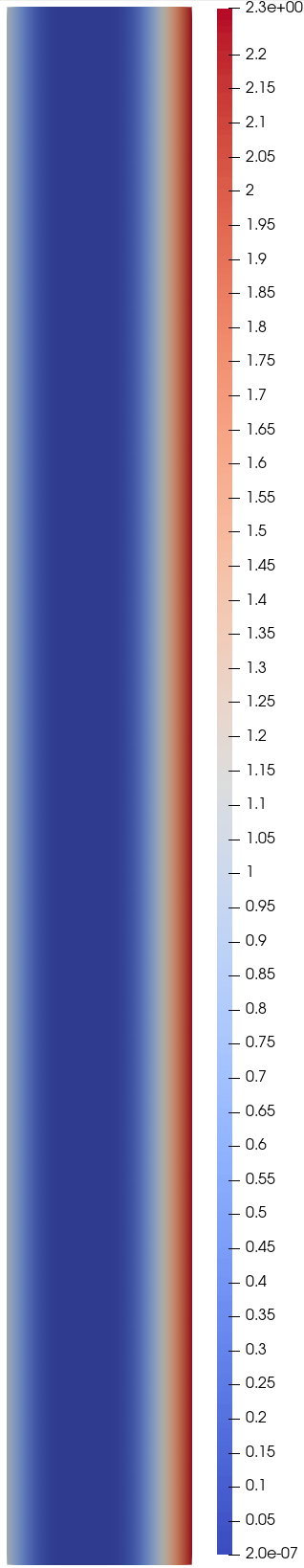
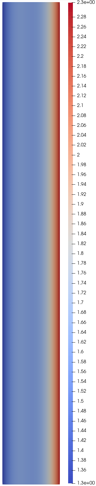
Figure 4: Annulus: left: $\Omega^{\prime}$ (red) and $\Omega\setminus\Omega^{\prime}$ (blue), middle: $|\mathcal{G}_{h,x}|^{2}$ and right: $|\mathcal{G}_{h,y}|^{2}$.

Indeed, in a large band in the middle of the domain, one can notice that $|\mathcal{G}_{h,x}|\simeq 0$. The violation of the constraints in $\Omega\setminus\Omega^{\prime}$ is interpreted as being the result of having gradient Dirichlet boundary conditions on all of $\partial\Omega$. Indeed, as stated in Remark 12, the constraints are not verified after the pattern fully folds on a curve, which corresponds to $|\varphi_{x}|=0$ and $|\varphi_{y}|=1$. As gradient Dirichlet boundary conditions are imposed on all of $\partial\Omega$, the pattern cannot relax in any part of the domain, as would have been possible with a part of the boundary having stress-free (homogeneous gradient Neumann) boundary conditions. This leads to an over-constrained pattern and thus to a solution that is not physical in some parts of the domain.

4.3 Axysymmetric surface

This example comes from [13]. The domain is $(0,2\pi)\times(0,4)$. A structured mesh, periodic in the $x$ direction, is used. The mesh has a size $h=0.126$ and contains $135,750$ dofs. The reference solution writes

$$\phi(x,y):=(\rho(y)\cos(x),\rho(y)\sin(x),z(x)),$$

where $\rho$ is a solution of

$$\ddot{\rho}=\frac{4\rho}{(4-\rho^{2})^{2}}.$$

An explicit Runge–Kutta method of order 5 (see [11]) is used to integrate this ODE with initial conditions $\rho_{0}=0.1$ and $\dot{\rho}_{0}=0$. Because the reference solution is not know analytically, the gradient Dirichlet boundary condition is imposed weakly using a least-squares penalty in order to remove numerical issues. Let $\mathcal{E}_{h}$ the set of the edges of $\mathcal{T}_{h}$. The set $\mathcal{E}_{h}$ is partitioned as $\mathcal{E}_{h}:=\mathcal{E}_{h}^{i}\cup\mathcal{E}_{h}^{b}$, where for all $e\in\mathcal{E}_{h}^{b}$, $e\subset\partial\Omega$ and $\cup_{e\in\mathcal{E}^{b}_{h}}{e}=\partial\Omega$. Let $h_{e}:=\mathrm{diam}(e)$, where $e\in\mathcal{E}_{h}$. Therefore, we search for $(\mathcal{G}_{h},r_{h})\in W_{h}\times R_{h}$,

$$\left\{\begin{aligned} &a(\mathcal{G}_{h};\mathcal{G}_{h},\tilde{G}_{h})+\mathfrak{p}(\mathcal{G}_{h},\tilde{G}_{h})+b(\tilde{G}_{h},r_{h})+\sum_{e\in\mathcal{E}^{b}_{h}}\frac{\eta}{h_{e}}\int_{e}\mathcal{G}_{h}:\tilde{G}_{h}\\ &=\sum_{e\in\mathcal{E}^{b}_{h}}\frac{\eta}{h_{e}}\int_{e}\mathcal{I}_{h}G_{D}:\tilde{G}_{h},\quad\forall\tilde{G}_{h}\in W_{h0},\\ &b(\mathcal{G}_{h},\tilde{r}_{h})=0,\quad\forall\tilde{r}_{h}\in R_{h}.\end{aligned}\right.$$

$5$ Newton iterations are necessary to reach converge.

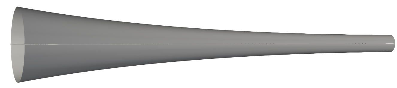
Figure 5: Axysymmetric surface: Computed surface.

Figure 5 shows the computed surface, which looks as expected in [13].

4.4 Deformed hyperboloid

The domain $\Omega$ is the same as in Section 4.1. A structured mesh, periodic in the $y$ direction, is used to mesh $\Omega$. The mesh has a size $h=0.089$ and contains $135,750$ dofs. The gradient Dirichlet boundary conditions are the same as in Section 4.1 for the left-hand side of $\Omega$ and rotated by $\frac{\pi}{6}$ radiants, with respects to Section 4.1, on the right-hand side of $\Omega$. This breaks the axial symmetry that allows one to reduce (1a) to an ODE. The Newton method converges after $5$ iterations. The resulting surface is presented in Figure 6.

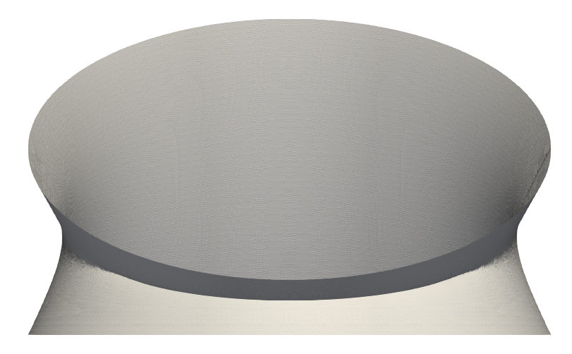
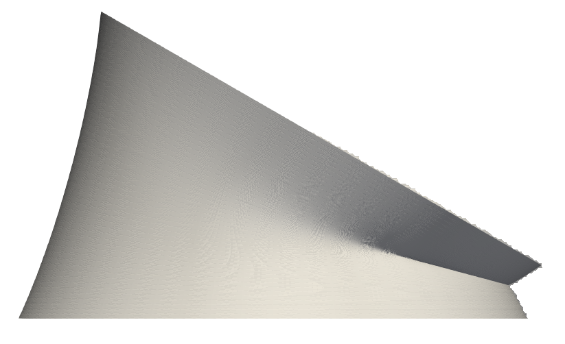
Figure 6: Deformed hyperboloid: Computed surface.

The inequality constraints (1d) are only verified in $\Omega^{\prime}\subsetneq\Omega$ for this test case, and thus, the equality constraints (1c) and (1b) are also only verified in $\Omega^{\prime}$.

5 Conclusion

In this paper, the existence of solutions to the constrained system of equations describing a Miura surface are proved under specific boundary conditions that still leave some freedom for design choices, see Figure 2. Then, a numerical method based on a mixed formulation, Taylor–Hood elements, and a Newton method is introduced to approximate Miura surfaces. The method is proved to converge in $H^{1}$ norm in the space discretization parameter $h$ and a convergence order of two is observed in practice. Some numerical tests are performed and show the robustness of the method. Future work includes studying the constrained nonlinear hyperbolic PDE derived by homogenizing the eggbox pattern, as in [17].

Code availability

The code is available at https://github.com/marazzaf/Miura.git

Funding

This work is supported by the US National Science Foundation under grant number OIA-1946231 and the Louisiana Board of Regents for the Louisiana Materials Design Alliance (LAMDA).

References

• [1] P. Badagavi, V. Pai, and A. Chinta. Use of origami in space science and various other fields of science. In 2017 2nd IEEE International Conference on Recent Trends in Electronics, Information & Communication Technology (RTEICT), pages 628–632. IEEE, 2017.
• [2] E. Boatti, N. Vasios, and K. Bertoldi. Origami metamaterials for tunable thermal expansion. Advanced Materials, 29(26):1700360, 2017.
• [3] H. Brézis. Functional analysis, Sobolev spaces and partial differential equations, volume 2. Springer, 2011.
• [4] P. G. Ciarlet. An introduction to differential geometry with applications to elasticity. Journal of Elasticity, 78(1):1–215, 2005.
• [5] M. Costabel and M. Dauge. Maxwell and lamé eigenvalues on polyhedra. Mathematical methods in the applied sciences, 22(3):243–258, 1999.
• [6] M. Dobrowolski and R. Rannacher. Finite element methods for nonlinear elliptic systems of second order. Mathematische Nachrichten, 94(1):155–172, 1980.
• [7] A. Ern and J.-L. Guermond. Theory and practice of finite elements, volume 159. Springer Science & Business Media, 2013.
• [8] D. Gallistl. Variational formulation and numerical analysis of linear elliptic equations in nondivergence form with Cordès coefficients. SIAM Journal on Numerical Analysis, 55(2):737–757, 2017.
• [9] D. Gilbarg and N. Trudinger. Elliptic partial differential equations of second order, volume 224. springer, 2015.
• [10] P. Grisvard. Elliptic problems in nonsmooth domains. SIAM, 2011.
• [11] E. Hairer, M. Hochbruck, A. Iserles, and C. Lubich. Geometric numerical integration. Oberwolfach Reports, 3(1):805–882, 2006.
• [12] R. J. Lang. Twists, tilings, and tessellations: mathematical methods for geometric origami. AK Peters/CRC Press, 2017.
• [13] A. Lebée, L. Monasse, and H. Nassar. Fitting surfaces with the Miura tessellation. In 7th International Meeting on Origami in Science, Mathematics and Education (7OSME), volume 4, page 811. Tarquin, 2018.
• [14] Frédéric Marazzato. $h^{2}$-conformal approximation of miura surfaces. Computational Methods in Applied Mathematics, 2023.
• [15] K. Miura. Proposition of pseudo-cylindrical concave polyhedral shells. ISAS report/Institute of Space and Aeronautical Science, University of Tokyo, 34(9):141–163, 1969.
• [16] J. Morgan, S. P. Magleby, and L. L. Howell. An approach to designing origami-adapted aerospace mechanisms. Journal of Mechanical Design, 138(5), 2016.
• [17] H. Nassar, A. Lebée, and L. Monasse. Curvature, metric and parametrization of origami tessellations: theory and application to the eggbox pattern. Proceedings of the Royal Society A: Mathematical, Physical and Engineering Sciences, 473(2197):20160705, 2017.
• [18] H. Nassar, A. Lebée, and L. Monasse. Macroscopic deformation modes of origami tessellations and periodic pin-jointed trusses: the case of the eggbox. In Proceedings of IASS Annual Symposia, volume 2017, pages 1–9. International Association for Shell and Spatial Structures (IASS), 2017.
• [19] J. Overvelde, T. A. De Jong, Y. Shevchenko, S. A. Becerra, G. M. Whitesides, J. C. Weaver, C. Hoberman, and K. Bertoldi. A three-dimensional actuated origami-inspired transformable metamaterial with multiple degrees of freedom. Nature communications, 7(1):1–8, 2016.
• [20] A. Rafsanjani, K. Bertoldi, and A. R. Studart. Programming soft robots with flexible mechanical metamaterials. Science Robotics, 4(29):eaav7874, 2019.
• [21] F. Rathgeber, D. Ham, L. Mitchell, M. Lange, F. Luporini, A. McRae, G.-T. Bercea, G. Markall, and P. Kelly. Firedrake: automating the finite element method by composing abstractions. ACM Transactions on Mathematical Software (TOMS), 43(3):1–27, 2016.
• [22] M. Schenk and S. Guest. Geometry of Miura-folded metamaterials. Proceedings of the National Academy of Sciences, 110(9):3276–3281, 2013.
• [23] I. Smears and E. Suli. Discontinuous Galerkin finite element approximation of nondivergence form elliptic equations with Cordès coefficients. SIAM Journal on Numerical Analysis, 51(4):2088–2106, 2013.
• [24] Z. Wei, Z. Guo, L. Dudte, H. Liang, and L. Mahadevan. Geometric mechanics of periodic pleated origami. Physical review letters, 110(21):215501, 2013.
• [25] A. Wickeler and H. Naguib. Novel origami-inspired metamaterials: Design, mechanical testing and finite element modelling. Materials & Design, 186:108242, 2020.