Revising the universality class of the four-dimensional Ising model

Abstract

The aim of this paper is to determine the behaviour of the specific heat of the 4-dimensional Ising model in a region aroud the critical temperature, and via that determine if the Ising model and the $\phi^{4}$-model belong to the same universality class in dimension 4. In order to do this we have carried out what is currently the largest scale simulations of the 4-dimensional Ising model, extending the lattices size up to $L=256$ and the number of samples per size by several orders of magnitude compared to earlier works, keeping track of data for both the canonical and microcanonical ensembles.

Our conclusion is that the Ising model has a bounded specific heat, while the $\phi^{4}$-model is known to have a logarithmic divergence at the critical point. Hence the two models belong to distinct universality classes in dimension 4.

I Introduction

The 4-dimensional Ising model is of special import for, at least, two reasons. First, it is at the boundary, known as the upper critical dimension, between the high-dimensional Ising models which follow mean-field behaviour and the low-dimensional cases $D=1,2,3$ each of which is qualitatively different from the others in just about every interesting property. Second, following the methods of constructive field theory a well-behaved, i.e.s̃atisfying certain axioms, 4-dimensional spin model corresponds to one or several, depending on a limit-taking procedure, time-dependent 3-dimensional quantum field theories. Hence a full understanding of the 4-dimensional Ising model is desirable both in order to complete our understanding of high-dimensional Ising models and as a necessary part of understanding time-dependent quantum-field theory in 3-dimensional space.

There are still many basic questions regarding this model which remain open. The broadest of these is arguably whether or not the Ising model for $D=4$ belongs to the same universality class as the $\phi^{4}$-model and, as a necessary condition for that inclusion, whether or not the specific heat of the Ising model has the same type of singularity as in the $\phi^{4}$-model.

Let us briefly recall that the lattice $\phi^{4}$-model is a spin model similar to the Ising model but instead of having spins $\pm 1$, as in the Ising model, the $\phi^{4}$-model allows all real numbers as spin values and the action, which we can think as the equivalent of the Hamiltonian in the Ising model, is $\beta\sum_{ij}(\phi_{i}-\phi_{j})^{2}+\sum_{i}(b\phi_{i}^{2}+\lambda\phi_{i}^{4})$, where $\phi_{i}$ is the spin at site $i$ and the first sum is over all nearest-neighbor pairs of sites. When restricted to spin values $\pm a$, for any constant $a$, the first sum is equivalent to the energy in the Ising model. For $\lambda>0,b<0$ the second term can be viewed as an energy contribution depending on how the spin-values deviate from $\pm\frac{\sqrt{-b}}{\sqrt{2\lambda}}$, as the summand is minimzed for $\phi_{i}=\pm\frac{\sqrt{-b}}{\sqrt{2\lambda}}$. Taking $b=-2\lambda$ and letting $\lambda\rightarrow+\infty$ we get a sequence of models with spin values increasingly concentrated around $\pm 1$, i.e., the spin values of the Ising model. Just like for the Ising model this energy is unchanged by a global change of sign of the spins.

Now, for the Ising model with $D=4$ the list of rigorous results is relatively short but still quite powerful. The inequalities of Sokal [1] show that for $D\geq 4$ the specific heat follows its mean field critical exponent, and for $D\geq 5$ it is bounded. For $D=4$ these inequalities do not prove that the specific heat is bounded, only that it cannot diverge faster than $\ln(|K-K_{c}|)$. Moreover the inequalities of [2, 3] show that for $K\geq K_{c}$ the magnetisation $M$ is bounded as $c_{1}\sqrt{K-Kc}\leq M\leq c_{2}(\ln(K-K_{c}))^{3/2}\sqrt{K-K_{c}}$, which also means that the magnetisation is continuous at $K_{c}$. For $K\leq K_{c}$ it has recently been proven [4] that, properly rescaled, the magnetisation converges to a Gaussian in the thermodynamic limit. However, the finite size critical region for the 4D-model with cyclic boundary lies in the interval $K>K_{c}$, see Ref. [5] for illustrations of how the location of the critical region varies with dimension and boundary condition, so this does cover all $L$-dependent finite size effective critical points. Non-rigorous results starting with [6] has predicted that for a class of models including the Ising model the specific heat should diverge as $(\ln|K-K_{c}|)^{1/3}$, but it has not been possible to turn this into a rigorous argument. The model has also been studied via series expansions of the specific heat and the susceptibility [7, 8, 9], mainly leading to estimates for $K_{c}$. However the authors of Ref. [10] attempts to estimate the exponent of $\ln|K-K_{c}|$ and cautiously note that this turns out to be difficult after getting an estimate much larger than $1/3$. Over the years, classical Monte Carlo metods have also been applied [11, 12, 13, 14] but the cost for simulation in $D=4$ has kept the lattice sizes down, with [13] reaching $L=40$ and [14] $L=60$. Most of these papers have estimated $K_{c}$ and simply concluded that a $(\ln|K-K_{c}|)^{1/3}$-divergence is compatible with the sampled data, but with no clear signal due to the limited range for $L$. However, in Ref. [14] we also took the microcanonical ensemble into account and found that this favored a scenario where the specific heat instead is bounded. Later papers have also applied numerical renormalisation techniques [15, 16].

For the $\phi^{4}$-model the rigorous results are today much more developed. The same non-rigorous results as for the Ising model [6] applies here and predicts the same divergent specific heat, as did later non-rigorous renormalisation arguments [17, 18]. The rigorous results from [1, 2, 3] also applies and proves that the mean-field exponents are correct. In 1989 Hara and Tasaki [19, 20] finally rigorously proved that the predicted logarithmic divergences are correct. Their results have since then been extended and reproven by additional techniques, and [21, 4] both provide good overviews of what is now known for this model.

Apart from the less well known Ref. [6] the advent of the concept of universality in the 1970’s led some authors — it is not clear if anyone can lay claim to be first — to state that the Ising model should have the exact same logarithmic divergence as the $\phi^{4}$-model when $D=4$. This claim is based on the fact that the family of models with the same spatial dimension and same symmetry group for the Hamiltonian, here given simply by sign-change for spins, form the simplest candidate for a universality class. Though Kadanoff did already in Ref. [22][Page 18] point out that this is merely the first approximation of the properties which define a universality class by adding to the list of defining properties: ”Perhaps other criteria”. The belief in a simple universality class was also strengthened by the rigorous proof in [23] of the fact that by partitioning the 2-dimensional square lattice into blocks and summing the spins inside each block to a block-spin value, we can build a sequence of spin models which converge, in a certain sense, to the 2-dimensional $\phi^{4}$-model. However, note that these block-spins are by construction always bounded in value, according to the block size, and the $\phi^{4}$-spins are unbounded. So here the exact definition of convergence is important and fluctuations in the approximating block-spins are in some sense always smaller than those in the limiting $\phi^{4}$-model.

Our aim in this paper is to investigate the critical behaviour of the 4-dimensional Ising model and, in addition to further sharpening estimates for the location of the critical point, find clear evidence for which universality class the model belongs to. We have done this by Monte Carlo simulation, keeping track of both microcanonical data and the usual canonical ensemble data. We have used lattices of size up to $L=256$, thus going far beyond earlier simulation studies. For each lattice size we have run simulations at $150$–$300$ temperatures, and typically several hundred independent spin systems of each size. In the coming sections we first give definitions, describe our sampling in more detail, and then proceed to analyze our data, first in the microcanonical and then the canonical ensemble, before finally coming to a discussion of our results.

II Definitions

The underlying graph is the four-dimensional (4D) $L\times L\times L\times L$ grid graph with periodic boundary conditions, i.e., the Cartesian graph product of $4$ cycles of length $L$, thus having $N=L^{4}$ vertices and $4L^{4}$ edges. On each vertex $i$ we place the spin $s_{i}=\pm 1$ and let the Hamiltonian with interactions of unit strength along the edges be $\mathscr{H}=\sum_{ij}s_{i}s_{j}$ where the sum is taken over the edges $ij$. As usual the coupling $K=1/k_{B}T$ is the dimensionless inverse temperature with $K_{c}$ the critical coupling.

The magnetisation of a state $s$ is $M=\sum_{i}s_{i}$ (summing over the vertices $i$) and the energy is $E=\sum_{ij}s_{i}s_{j}$ (summing over the edges $ij$), let also $m=M/N$ and $U=E/N$. With the partition function $Z(K)=\sum_{s}e^{KE(s)}$ we can now define the standard quantities and indicate how they can be measured. The internal energy is as usual

$$\operatorname{\mathcal{U}}=\frac{1}{N}\frac{\partial\ln Z}{\partial K}=\frac{\left\langle E\right\rangle}{N}$$ (1)

where $\left\langle\cdots\right\rangle$ is the thermal-equilibrium mean. The specific heat for a graph on $N$ vertices is defined as

$$\operatorname{\mathcal{C}}=\frac{1}{N}\frac{-\partial^{2}\ln Z}{\partial T\partial K}=\frac{K^{2}}{N}\mathrm{var}\!\left(E\right)$$ (2)

The energy excess kurtosis (or simply, kurtosis) is a ratio of cumulants, or, a translated ratio of central moments

$$\operatorname{\mathcal{G}}=\frac{\partial^{4}\ln Z/\partial K^{4}}{\left(\partial^{2}\ln Z/\partial K^{2}\right)^{2}}=\frac{\left\langle\left(E-\left\langle E\right\rangle\right)^{4}\right\rangle}{\mathrm{var}\!\left(E\right)^{2}}-3$$ (3)

The data are collected in a micro-canonical fashion so that all measurements are associated with the energy level $E$. A crucial quantity to measure is $R(E,\Delta E)$, defined as the probability at energy $E$, that the energy changes by $\Delta E$ when a spin, selected uniformly at random, is flipped. Recall that for the spin at vertex $i$ the energy changes by $\Delta E=-2s_{i}\sum_{ij}s_{j}$ (summing over the edges with one end in vertex $i$).

Let us briefly go through the micro-canonical details. With each $K$ we associate an energy corresponding to the maximum term in the partition function $Z(K)=\sum_{E}w(E)e^{KE}$, where $w(E)$ is the number of states at energy $E$. Then

$$w(E-\Delta E)e^{K(E-\Delta E)}<w(E)e^{KE}>w(E+\Delta E)e^{K(E+\Delta E)}$$ (4)

leading to the relation, for $\Delta E>0$,

$$\frac{1}{\Delta E}\ln\frac{w(E-\Delta E)}{w(E)}\leq K\leq\frac{1}{\Delta E}\ln\frac{w(E)}{w(E+\Delta E)}$$ (5)

and we choose the average of the end-points as the value for $K$

$$\operatorname{K}(U)=\frac{1}{2\Delta E}\ln\frac{w(E-\Delta E)}{w(E+\Delta E)},\quad U=E/N$$ (6)

With the (micro-canonical) entropy defined as $\operatorname{S}(U)=(1/N)\ln w(E)$, for $U=E/N$, its discrete derivative can now be written as

$$\operatorname{S}^{\prime}(U)=\frac{\operatorname{S}(U+\Delta E/N)-\operatorname{S}(U-\Delta E/N)}{2\Delta E/N}=-\operatorname{K}(U)$$ (7)

Since $w$ and $R$ are related through the micro-canonical form of detailed balance

$$w(E)\,R(E,\Delta E)=w(E+\Delta E)\,R(E+\Delta E,-\Delta E)$$ (8)

we can now, using Eq. (6), give an alternative definition of the $\operatorname{K}$-function in terms of $R$

$$\operatorname{K}(U)=\frac{1}{\Delta E}\ln\frac{R(E,-\Delta E)}{R(E,\Delta E)},\quad U=E/N,\,\Delta E>0$$ (9)

where the approximation $R(E,\Delta E)\approx R(E+\Delta E,\Delta E)$ has been used implicitly [24]. Note that for 4D systems a single spin-flip gives only $-16\leq\Delta E\leq 16$ and thus this approximation is safe except for very small graphs. Note also that there are four positive values of $\Delta E$ to choose from ($4,8,12,16$) so we have in fact used a weighted average of the four possible candidates for $\operatorname{K}(E)$ leading to a small improvement in data quality. This is in fact the only form of smoothing our data have been subjected to.

From $\operatorname{K}(U)$ we can now reconstruct the canonical energy distribution for any $K$ as follows

$$\Pr(E)=A\exp\left\{N\int_{u}^{U}\exp\left[K-\operatorname{K}(x)\right]\,\mathrm{d}x\right\}$$ (10)

where $U=E/N$ and the constant $A$ is implicitly defined by $\sum_{E}\Pr(E)=1$. The lower bound $u$ in the integral is simply the smallest $U$ for which we have data. Ideally one should measure $R$ for all $-4L^{4}\leq E\leq 4L^{4}$ but this is not practical for the larger systems. One simply measures at a well-chosen range of $E$ such that the energy distribution of Eq. (10) fits within, say, four or five standard deviations from the end-points of the collected data range. A detailed discussion of these rather technical considerations, with worked examples, can be found in Refs. [24, 25].

Finally, the normalised coupling is denoted by $\varepsilon=(K-K_{c})/K_{c}$ and the rescaled coupling is $\kappa=L^{2}\varepsilon$. From time to time we will also consider an alternative log-corrected form, $L^{2}(\ln L)^{1/6}\varepsilon$. A phenomenologically critical point is denoted $K_{c}(L)$ or simply $K^{*}$ depending on context, analogously we write $\varepsilon^{*}$ and $\kappa^{*}$. When a quantity depends on $L$ we will subscript it, as in for example $\operatorname{\mathcal{C}}_{L}(K)$, and usually let $\operatorname{\mathcal{C}}(K)$ refer to the asymptotic function (in the thermodynamic limit) when $L\to\infty$.

III Ensemble equivalence

Since the main evidence for our final conclusion comes from the microcanonical ensemble, while the canonical ensemble is the one most commonly used, we will first review the rigorous results on ensemble equivalence.

Equivalence results have in the past been proven for various models, varying assumptions, and different versions of equivalence. However, more recently these results were proven in a rigorous and unified way in Ref. [26]. There it is proven that, assuming that the thermodynamic limit of the model exists and is non-trivial, the canonical and microcanonical ensembles are equivalent if and only if the entropy $S(U)$ has a global supporting line at every point $U$ in the support of $S$. Here a global supporting line at a point $U_{0}$ line is a tangent line for the graph at $S(U_{0})$ which does not intersect the graph at any other point. In particular, such supporting lines exist if $S$ is a strictly concave function. Note that this theorem requires no other assumptions about the model or exact behaviour at phase transitions.

If the ensembles are not equivalent it follows that $S(U)$ is not a strictly concave function. This in turn means that the mode must have meta-stable states for some temperature and a first-order phase transition at that point. The connection to first-order transitions is nicely surveyed in Ref. [27].

Looking at the Ising model in four dimensions we can quickly rule out a first-order phase transition. Recall that at a first-order phase transition the energy variance is unbounded, since the model jumps between two states with macroscopically different energies $U_{-}$ and $U_{+}$, so the only point where this could potentially happen is at the usual critical point of our model. However, as already mentioned the rigorous results of Refs. [2, 3] show that the magnetisation of our model is a continuous function, thereby ruling out a first-order phase transition. So, for the 4-dimensional Ising model we have ensemble equivalence.

We will now make this more quantitative. For finite $N$ the free energy $\operatorname{\mathcal{F}}(K)=(1/N)\ln Z(K)$ satisfies $\operatorname{\mathcal{F}}(K)\geq(1/N)\ln(w(E)e^{KE})$ for all $E$, in particular for the maximum term at $E$ associated with $K$, that is, $\operatorname{\mathcal{F}}(K)\geq KU+S(U)$ where $U=E/N$. In the thermodynamic limit $N\rightarrow\infty$ $\operatorname{\mathcal{F}}(K)$ is given by the Legendre-Fenchel transform of $-S(U)$, that is, $\operatorname{\mathcal{F}}(K)=\sup_{U}\{KU-(-S(U))\}$, since we have equivalence of the canonical and microcanonical ensembles for the model.

To be precise, the condition of strict concavity means that if $S(U)$ is twice differentiable the ensembles are equivalent if

$$-\frac{(S^{\prime}(U))^{2}}{S^{\prime\prime}(U)}\geq 0,$$ (11)

with equality in at most one value of $U$. In the thermodynamic limit this is a condition on the specific heat, since

$$\operatorname{\mathcal{C}}(K)=K^{2}\frac{\partial\operatorname{\mathcal{U}}}{\partial K}=\frac{\operatorname{K}(U)^{2}}{\partial\operatorname{K}/\partial U}=\frac{\operatorname{K}(U)^{2}}{\operatorname{K}^{\prime}(U)}=-\frac{(S^{\prime}(U))^{2}}{S^{\prime\prime}(U)}$$ (12)

Now let us assume that for $K$ close to $K_{c}$ and $U$ close to $U_{c}$ we have that $\operatorname{\mathcal{C}}(K)=f(K_{c}-K)$ for some function $f$, which has a singularity of some form at 0. Now using Equation 12 and the fact that $\operatorname{K}(U_{c})=K_{c}$ this leads to

$$\operatorname{K}^{\prime}(U)=\frac{(K_{c}+o(1))^{2}}{f(K_{c}-K)}.$$

Here we see that the specific heat is divergent at $K_{c}$ if and only if $\operatorname{K}^{\prime}(U)\to 0$ when $U\to U_{c}$. The exact form of the divergence, e.g. power-law or logarithmic, will only influence how quickly $\operatorname{K}^{\prime}(U)\to 0$ for $U$ close to $U_{c}$. Similarly the specific heat will have a jump discontinuity if and only if $\operatorname{K}^{\prime}(U)$ has one a well.

For a sequence of finite systems this in turn means that in order for the maximum of the specific heat to diverge as $L$ increases, the minimum value of $\operatorname{K}_{L}^{\prime}(U)$ must go to 0, as otherwise there would be a strictly positive lower bound on the value of $\operatorname{K}^{\prime}(U)$

While these results demonstrate how the asymptotic, thermodynamical, limits of the microcanonical and canonical ensembles connect do not give us a simple connection between their finite-size approach to the thermodynamical limits. For the canonical ensemble the finite-size behaviour is a combination of the finite size effects for the microcanonical density of states at individual energies, plus the fact that the number of distinct energies grows with the system size, and how strongly the exponential reweighting of the microcanonical states concentrates the internal energy for given $K$ on a specific value of $U$. The latter can e.g. lead to an increase in the specific heat even if there are no finite-size effects at all in the values of $S(U)$ for those $U$ which correspond to existing values of $E$ for finite $N$. Over all, finite size effects for the canonical ensemble are expected be more complex than for the micronanonical.

IV Sampling and data analysis

We have collected data for $L=6$, $8$, $10$, $12$, $16$, $20$, $24$, $32$, $40$, $48$, $56$, $64$, $80$, $96$, $112$, $128$, $160$, $192$ and $256$ using standard Wolff-cluster updating [28] for generating states in combination with the Mersenne-twister random-number generator [29].

The data are collected over an interval of energies covering all points of phenomenological interest, such as maximum kurtosis and specific heat. This is then a data window of particular interest where we have the largest number of measurements per energy level. When converting from micro-canonical to canonical form in this window we do so at $\kappa$-steps of length $\approx 0.05$. Outside this window we use larger step lengths, usually at most $0.25$. This typically means that the various quantities are evaluated at $150$–$300$ different temperatures depending on system size. For temperatures between these steps we use standard third-order interpolation, thus effectively giving us a continuum of temperatures.

The number of measurements per energy level vary considerably between system sizes, for the smaller systems typically $10^{4}$–$10^{6}$, but this number decreases quickly and for the largest systems it is only $10$–$50$. The number of energy levels in the window of interest also increases with $L$ so the total number of measurements is still large. Keep in mind that the data are not smoothed at all (except for an average taken in connection with Eq. (9)) which means that the $\operatorname{K}$-function is quite noisy. However, the distribution resulting from applying Eq. (10) to the $\operatorname{K}$-function is very smooth and well-behaved, since the noise is uncorrelated and hence mostly canceled out by the integral. Once this distribution has been computed it is of course easy to compute the weighted averages the canonical quantities are made of.

This method produces very smooth canonical data, even though the unsmoothed micro-canonical data appear noisy. Still, some mild noise will show up in high- or low-temperature regions for higher-order cumulants, especially for the largest systems. Inside the scaling window such quantities usually are considerably more stable.

However, as mentioned in the discussion of ensemble equivalence the error for a canonical quantity is a mixture of the errors for the microcanonical data, meaning that we do not get a simple formula for these errors. Having said that, an indirect estimate of any error can be obtained based on the Monte Carlo data gathered at a few temperatures close to $K_{c}$ for some of the larger systems. For example, for $L=256$ (and most of the larger $L$) we have roughly 2 million measurements at each of these temperatures. From standard bootstrap estimates of these data we find the error of the energy $\operatorname{\mathcal{U}}$ to be less than $2\times 10^{-7}$ and for the specific heat $\operatorname{\mathcal{C}}$ we estimate the error to be less than $0.003$. Thus, for these temperatures, we can use the raw Monte Carlo data for comparison to our micro-canonical data. Concretely we have found the largest difference in the specific heat for $L=256$, to be 0.8% of the estimated value. The error for most temperatures and $L=96,\ldots,256$ is typically in the range 0.1-0.6%. For the internal energy the largest error was $2\times 10^{-6}$, but more typically a magnitude smaller, for $L\geq 80$. For smaller lattices both the specific heat and internal energy have negligible errors. Hence we choose not to print error bars in our figures.

We also expect that any error will show up as noise over an interval of $K$, or that a sequence of system sizes will flush out any culprit system that appears off in a finite-size scaling fit. We are particularly on the look-out for trends in the error, say if the difference between the points and the fitted curve increases with $L$, always a sign that the ansatz curve is not correctly chosen. Often there are higher-order corrections at play, so that the fitted curve is only relevant for larger $L$. To guard against this we use the standard technique of fitting the curve to a range of $L$ beginning at $L_{\min}$, then repeat the fit by increasing $L_{\min}$. So, if the ansatz is a curve of the form $A_{0}+\frac{A_{1}}{L^{p}}$ we can take the median or mean of the $A_{0}$ and $A_{1}$ and use their respective interquartile range or standard deviation as error estimates (choosing, say, the largest). To conclude, we check against trends in $L$ and often estimate error bars in several different ways. This is a more qualitative and, we think, relevant approach to data analysis than simply using reduced $\chi^{2}$-estimates of the error, especially when non-linear data are involved [30].

V Micro-canonical quantities

The micro-canonical density of states is of course fundamental to the model and determines the behaviour of the canonical distribution. Fig. 1 demonstrates this in the case of $L=64$, showing both $\operatorname{K}_{L}(U)$ and its derivative $\operatorname{K}_{L}^{\prime}(U)$, together with the energy distributions for two temperatures of interest, $K_{c}$ and at the $K_{c}(L)$ corresponding to the maximum specific heat. This figure is quite representative for all $L\geq 6$. For example, the distribution at $K_{c}$ is sharply skewed to the left, somewhat off-center from the minimum $\operatorname{K}^{\prime}(U)$. At $K_{c}(L)$ on the other hand, the distribution has a more symmetric look. All this is of course governed by the $\operatorname{K}$-curve. Other phenomenological critical points occur at other places giving rise to distributions of other shapes. For the purpose of this plot the $\operatorname{K}_{L}$- and $\operatorname{K}_{L}^{\prime}$-curves have here been smoothed, using a standard moving-window average of width corresponding to half the standard deviation of the energy at $K_{c}(L)$.

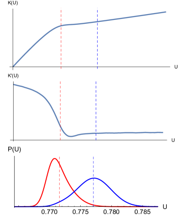
Figure 1: (Colour on-line) $\operatorname{K}_{L}(U)$ (top), $\operatorname{K}_{L}^{\prime}(U)$ (middle) and $\Pr(U)$ (bottom) plotted versus $U$ for $L=64$. All three figures cover the same interval of $U$. The bottom figure shows the distribution of energies for $K=K_{c}$ (left) and for $K^{*}$ (right) giving the maximum specific heat. The dashed lines show the mean energy, $\operatorname{\mathcal{U}}(K)$, for the respective distribution (or $K$). This picture is representative for all $L\geq 6$ regarding the shape of the distributions and their location in relation to the minimum in $\operatorname{K}_{L}^{\prime}(U)$.

In Figs. 2 and 3 we plot $\operatorname{K}_{L}(U)$ and $\operatorname{K}_{L}^{\prime}(U)$ respectively for a range of $L$ to show how they evolve to a limit curve. Piecing together a sequence of $\operatorname{K}$- and $\operatorname{K}^{\prime}$-curves, according to where their values agree with those for larger $L$, gives an approximation of their asymptotic limit and are shown in Figs. 4 and 5. Note that, as seen in the inset of Fig. 4 this approximation will not give a curve very close to the critical point, since the data from the largest value of $L$ cannot be compared to a larger size. In the second figure we have also included data from Padé-approximants based on the high- and low-temperature series expansions of the free energy [7, 8, 9].

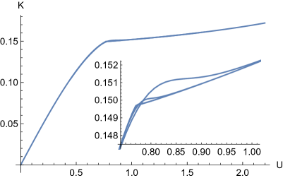
Figure 2: (Colour on-line) Function $\operatorname{K}_{L}(U)$ plotted versus $U$ for $L=8$, $16$, $32$, $64$, $128$. Inset shows a zoomed in plot. The curves are smoothed.

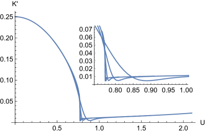
Figure 3: (Colour on-line) Function $\operatorname{K}_{L}^{\prime}(U)$ plotted versus $U$ for $L=8$, $16$, $32$, $64$, $128$. Inset shows a zoomed in plot. The curves are smoothed.

Of particular interest here is of course the minimum value of $\operatorname{K}_{L}^{\prime}(U)$ and these are shown in Fig. 6. We have in this plot attempted a simple scaling rule for these points, $y=A_{0}+A_{1}/L^{2}$ fitted to $L\geq 8$, which appear largely correct, despite the presence of some noise. We estimate a limit value of $A_{0}=0.00371(8)$ and the slope $A_{1}=-0.098(1)$. The error bar for $A_{0}$ is here the mean difference between the line and the points and for $A_{1}$ the standard deviation of the fitted slopes when deleting one point. Here we work under the assumption that the model does not have a finite-size effect so large that the minimum $\operatorname{K}^{\prime}(U)$ begins to decrease for some $L>256$.

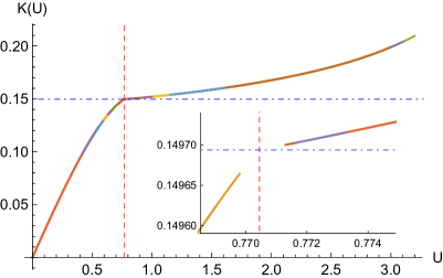
Figure 4: (Colour on-line) Limit curve $\operatorname{K}(U)$ plotted versus $U$. Pieced together from smoothed $\operatorname{K}_{L}(U)$ for $6\leq L\leq 256$ (different colours). The dashed vertical line is at $U_{c}$ and the horisontal dot-dashed line at $K_{c}$. Inset shows a zoomed in plot.

In our earlier study [14] we only had data for $L\leq 80$ and used $A_{1}/L$ as correction term but with these new data that correction term does not fit as well as $A_{1}/L^{2}$. However, the result is qualitatively the same: the minimum value is increasing with $L$ and, more importantly, the limit is distinctly positive.

As a technical point we note that care must be taken when finding the minimum $\operatorname{K}^{\prime}_{L}$. We have fitted a $7$th degree polynomial to the unsmoothed $\operatorname{K}_{L}(U)$-data over a $U$-interval where it preserves the shape and profile of the $\operatorname{K}_{L}^{\prime}(U)$-curves for different $L$. This interval is of course easily recognized by comparing the derivative of the polynomial to the smoothed $\operatorname{K}_{L}^{\prime}$-curves.

Recall that in the thermodynamic limit Eq. (12) derives the maximum specific heat from the minimum value of the $\operatorname{K}_{L}^{\prime}(U)$-curve. However, here the order of the limits is crucial; the limit of the minima for finite $L$ is not necessarily equal to the minimum of the limiting curve. Such examples are known already from the 2D Ising model. If we look at the sequence of curves in Fig. 3 we see that to the right of the critical point the curves step by step agree on a curve which seems to lie noticeably higher than the sequence of minima. From the rough asymptotic curve given in Fig. 5 we see that the curve does bend down close to the critical point and we can give 0.008 as a, very, rough upper bound on the asymptotic minimum, while $A_{0}$ of course provides a lower bound.

Following Eq. (12) this would imply that the limit maximum specific heat, given by $K_{c}^{2}/(\min\operatorname{K}^{\prime})$ is bounded by $0.1496^{2}/0.008\approx 2.8\lesssim\operatorname{\mathcal{C}}_{\infty}\lesssim 0.1496^{2}/0.0037\approx 6.03$. Since these two bounds are based strictly on the values to the right of $U_{c}$ they are also bounds on the limit of $\operatorname{\mathcal{C}}_{\infty}$ from the low-temperature side. Using the rough upper bound of $0.05$ for the left side limit of $\operatorname{K}^{\prime}$ we find $0.1496^{2}/0.05\approx 0.448$ to be a lower bound on the limit of $\operatorname{\mathcal{C}}_{\infty}$ from the high-temperature side, while the global bound provides an upper bound.

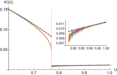
Figure 5: (Colour on-line) Limit curve $\operatorname{K}^{\prime}(U)$ plotted versus $U$. Pieced together from smoothed $\operatorname{K}_{L}^{\prime}(U)$ for $6\leq L\leq 256$ (different colours). The dashed vertical line is at $U_{c}$. The dashed black curve is obtained from series expansions. Inset shows a zoomed in plot of the low-temperature case.

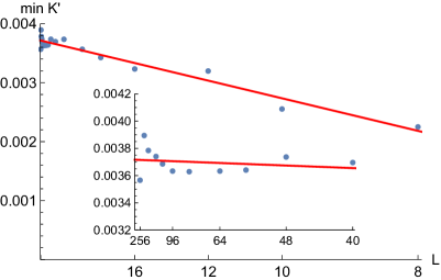
Figure 6: (Colour on-line) Minimum $\operatorname{K}_{L}^{\prime}(U)$ plotted versus $1/L^{2}$ for $L=8,\ldots,256$. The fitted red line is $y=0.00371(8)-0.098(1)x$ where $x=1/L^{2}$. The inset shows a zoom-in for $L=40,\ldots,256$.

It is of some interest to also consider $K_{c}(L)$, defined as the value of $\operatorname{K}$ at this $\operatorname{K}^{\prime}$-minimum, see Fig. 7. We find $K_{c}(L)=0.14969383(6)+0.1143(2)/L^{2}$ (fitting to $L\geq 64$) with error bars obtained as above; mean distance between points and line, and, slope variation when deleting each point in turn. Higher-order corrections become relevant for $L<64$. As we will see later this estimate of $K_{c}$ is consistent with what we will find from the canonical quantities.

Figure 7: (Colour on-line) The value of $\operatorname{K}_{L}$ at minimum $\operatorname{K}_{L}^{\prime}(U)$, or $K_{c}(L)$, plotted versus $1/L^{2}$ for $L=64$, $80$, $96$, $112$, $128$, $160$, $192$, $256$. The red line, fitted to these points, is $y=0.14969383(6)+0.1143x$ where $x=1/L^{2}$. The inset shows $(K_{c}(L)-0.14969383)L^{2}$ versus $L$ for $L\geq 16$ and the constant line $y=0.1143$.

Finally, the location $U_{L}$ of the minimum $\operatorname{K}_{L}^{\prime}(U)$ is shown in Fig. 8. We find $U_{L}=0.77048(1)+10.60(4)/L^{2}$, obtained in the same way as the scaling for $K_{c}(L)$ above, thus giving us an estimate of $U_{c}$. Note that the inset of the figure shows that $L=256$ deviates slightly from the line, but this $L$ also has more noise than the smaller cases.

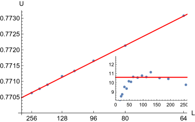
Figure 8: (Colour on-line) The value $U_{c}(L)$ giving minimum $\operatorname{K}_{L}^{\prime}(U)$ plotted versus $1/L^{2}$ for $L=64$, $80$, $96$, $112$, $128$, $160$, $192$, $256$. The red line, fitted to these points, is $y=0.77048(1)+10.60x$ where $x=1/L^{2}$. Inset shows $(U_{c}(L)-0.77048)L^{2}$ versus $L$ for $L\geq 16$ and the constant line $y=10.6$.

VI Canonical properties: Finite-size scaling for the specific heat

We now turn to the properties of the model in the better known canonical ensemble. We will first test two scenarios for the finite-size scaling of the specific heat at, or near, $K_{c}$. These are in turn based on two distinct asymptotic behaviours for the specific heat, either it is bounded as in the pure mean-field model, or it has a poly-log divergence of the same type as the $\phi^{4}$-model. A challenge for earlier studies has been to distinguish between these distinct asymptotics due to the slow growth in the second scenario.

In the first scenario, where we assume that the specific heat is bounded, we use a very simple scaling rule: $\operatorname{\mathcal{C}}_{L}(K_{c})=A_{0}+A_{1}/L^{a}$. This turns out to give a good first estimate of $K_{c}$ as a bonus. In Fig. 9 we show this for $a=1/5$ using $K_{c}=0.14969378$. The points that bend upwards and downwards shows the same sequence for $K_{c}\pm 5\times 10^{-7}$. In fact, this effect is clear already for changes in $K_{c}$ as small as $1.5\times 10^{-7}$. This sensitvity is obtained for a wide range of $a<1$. Thus, so far we have $K_{c}=0.14969378(15)$.

However, the corrections to scaling $(\operatorname{\mathcal{C}}_{L}(K_{c})-A_{0})L^{a}$ can give us a clearer picture as to the quality of the fitted scaling. Plausible fits to the points (not shown here) can be made for $a=1/6$ and $1/4$ (if we stay with the simple rationals) only with differently signed corrections for small $L$. Outside this range the corrections look less convincing. We find that the best fit is found for $a=1/5$ using $K_{c}=0.14969378(1)$ where the error bar indicates the interval where the corrections look similar to the inset plot of Fig. 9. Note that there are only very weak corrections for small $L$ and some larger deviations for $L=192$ and $256$. Fitting on $L_{\min}\leq L\leq 256$ for $20\leq L_{\min}\leq 64$ gives the asymptotic specific heat at $K_{c}$ being $A_{0}=1.837(3)$ and the correction coefficient $A_{1}=-1.24(1)$. The $A_{0}$-value is of course highly dependent of $a$. Choosing $a=1/6$ gives $A_{0}\approx 1.94$ and $a=1/4$ gives $A_{0}\approx 1.74$ when fitting on $L\geq 64$.

Let us also here mention that the global maximum of the specific heat is excellently fitted by $\max\operatorname{\mathcal{C}}_{L}=4.378(3)-3.472(9)/L^{1/5}$ with error bars from fitting over $L$-ranges with $20\leq L_{\min}\leq 64$.

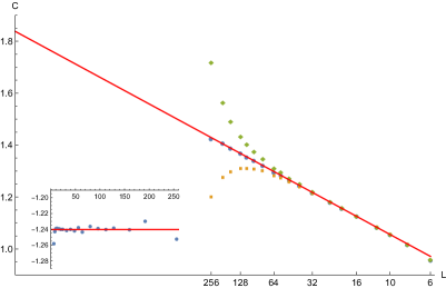
Figure 9: (Colour on-line) Specific heat $\operatorname{\mathcal{C}}_{L}(K_{c})$ versus $1/L^{1/5}$ for $L=6,8,\ldots,256$ and the fitted line $y=1.838(3)-1.24(1)x$ where $x=1/L^{1/5}$. Here we use $K_{c}=0.14969378$. The other points are $\operatorname{\mathcal{C}}_{L}$ at $K_{c}+5\times 10^{-7}$ (diamonds, bending upwards) and $K_{c}-5\times 10^{-7}$ (squares, bending downwards). Inset shows correction to scaling $(\operatorname{\mathcal{C}}_{L}(K_{c})-1.838)L^{1/5}$ versus $L$ and the constant line $y=-1.24$.

The second scenario, based on calculations for the $\phi^{4}$-model [31, 32, 33], is

$$\operatorname{\mathcal{C}}_{L}(K_{c})=B_{0}+B_{1}(\ln L)^{1/3}+B_{2}\frac{\ln\ln L}{(\ln L)^{2/3}}$$ (13)

In Fig. 10 we show $\operatorname{\mathcal{C}}_{L}(K_{c})$ versus $L$ with $K_{c}=0.149693785$. To these points we fit Eq. (13), finding $B_{0}=-0.15(1)$, $B_{1}=0.849(1)$ and $B_{2}=0.15(1)$ (error bars from different point ranges). The two other point sets in the figure shows the values for $K_{c}\pm 5\times 10^{-7}$, thus clearly giving an interval for $K_{c}$. In fact, the effect is visible for $\pm 1\times 10^{-7}$. The error in the fit is less than $0.001$ for $8\leq L\leq 192$. Hence, the second scenario, having the same number of parameters as the first, also results in a good fit.

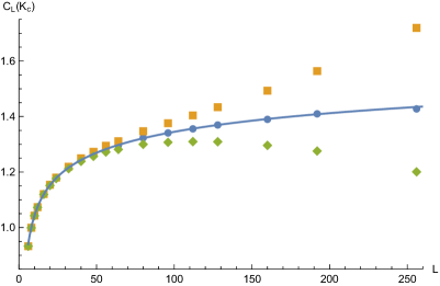
Figure 10: (Colour on-line) Specific heat $\operatorname{\mathcal{C}}_{L}(K_{c})$ versus $L$ for $L=6,8,\ldots,256$ and the fitted curve $y=-0.15+0.849(\ln L)^{1/3}+0.15\frac{\ln\ln L}{(\ln L)^{2/3}}$ for the points at $K_{c}=0.149693785$. The other points are $\operatorname{\mathcal{C}}_{L}$ at $K_{c}+5\times 10^{-7}$ (orange squares, bending upwards) and $K_{c}-5\times 10^{-7}$ (green diamonds, bending downwards).

In the next section we make use of the two scaling scenarios to test their respective scenario for the thermodynamic limit of the model.

VII The asymptotic specific heat: Two scenarios

We will now test the two main scenarios for the behaviour of the specific heat close to $K_{c}$ in the thermodynamic limit: a) that, like for higher dimensions $d\geq 5$ [34], it follows mean-field behaviour: taking a left-limit value for $\varepsilon\to 0^{-}$, another value for $\varepsilon=0$, and a right-limit value for $\varepsilon\to 0^{+}$, with some singular exponents $\theta^{-}$ and $\theta^{+}$ guiding the behaviour for small values of $|\varepsilon|$, or, b) that it behaves as the $\phi^{4}$-model [32, 33], i.e., $C(\varepsilon)\sim(-\ln(|\varepsilon|))^{1/3}$.

VII.1 The high-temperature range

In order to test the scenarios we will first construct an asymptotic ($L\to\infty$) $\operatorname{\mathcal{C}}$-curve. This can be obtained by piecing together $\operatorname{\mathcal{C}}_{L}$-data, for a sequence of $L$, proceeding like in Ref. [34]. In more detail, $\operatorname{\mathcal{C}}_{6}(K)$ and $\operatorname{\mathcal{C}}_{8}(K)$ are effectively equal (modulo noise) for $K\leq 0.11$, determined by ocular inspection with some safety margin, so $\operatorname{\mathcal{C}}_{6}(K)$ can now be treated as the asymptotic $\operatorname{\mathcal{C}}(K)$-curve when $K\leq 0.11$. Next, $\operatorname{\mathcal{C}}_{8}(K)$ and $\operatorname{\mathcal{C}}_{10}(K)$ are effectively equal for $K\leq 0.125$, so $\operatorname{\mathcal{C}}_{8}(K)$ can be treated as $\operatorname{\mathcal{C}}(K)$ for $K\leq 0.125$, etc. Continuing like this all the way up to $\operatorname{\mathcal{C}}_{160}(K)$ for $K\leq 0.14965$ (our $\operatorname{\mathcal{C}}_{L}$-data for $L=192$ and $L=256$ unfortunately do not overlap those for $L=160$) we have built up a limit $\operatorname{\mathcal{C}}(K)$-curve for $0\leq K\leq 0.14965$, or preferably, $\operatorname{\mathcal{C}}(\varepsilon)$ for $-1\leq\varepsilon\lesssim-0.00029$. In Fig. 11 we show the resulting asymptotic curve $\operatorname{\mathcal{C}}(\varepsilon)$ together with an inset demonstrating how some of the $\operatorname{\mathcal{C}}_{L}$-curves overlap.

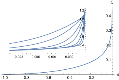
Figure 11: (Colour on-line) Asymptotic specific heat $\operatorname{\mathcal{C}}(\varepsilon)$ versus $\varepsilon$ for high temperatures. Inset shows $\operatorname{\mathcal{C}}_{L}$ versus $\varepsilon$ for $L=6$, $8$, $12$, $16$, $24$, $32$, $48$, $64$, $96$. Asymptotic curve $\operatorname{\mathcal{C}}_{\infty}$ built from piecing together $\operatorname{\mathcal{C}}_{L}$ for $6\leq L\leq 192$.

Fitting the asymptotic curve to a simple formula $y=A_{0}+A_{1}(-\varepsilon)^{\theta^{-}}$ over $-0.04<\varepsilon$ gives $\theta^{-}=0.1035(5)$ with $A_{0}=0.807(1)$ and $A_{1}=-0.861(1)$. Adjusting the lower bound between $-0.02$ and $-0.05$ gives parameters varying only very slightly, thus providing us with quite narrow error bars. The resulting curve is shown in Fig. 12. As the inset plot shows the relative error of such a fit is small and shows no clear trend. In Fig. 13 we show $0.807-\operatorname{\mathcal{C}}(\varepsilon)$ versus $-\varepsilon$ in a log-log plot together with the line $y=\ln(0.861)+0.1035x$ to demonstrate its linear behaviour.

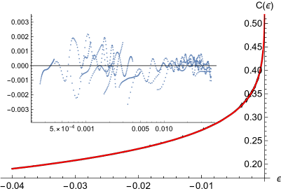
Figure 12: (Colour on-line) Asymptotic specific heat $\operatorname{\mathcal{C}}(\varepsilon)$ and the fitted curve $y=0.807-0.861(-\varepsilon)^{0.1035}$ (indistinguishable) versus $\varepsilon$. Inset shows relative error $(y-\operatorname{\mathcal{C}})/\operatorname{\mathcal{C}}$ versus $\ln(-\varepsilon)$.

Of course, if we narrow the fitted interval still further the parameters will change, but only very little. For example, with $-0.01<\varepsilon$ the curve becomes $y=0.821-0.870(\-\varepsilon)^{0.100}$, but the relative error will then grow larger at $\varepsilon=-0.04$. On a more global scale the specific heat should then take an almost linear behaviour when plotting $A_{0}-\operatorname{\mathcal{C}}(\varepsilon)$ versus $-\varepsilon$ in a log-log plot, see Fig. 13. Of course, choosing different values of $A_{0}$ will change the picture, becoming visibly non-linear for $A_{0}<0.7$ and $A_{0}>1.1$.

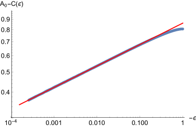
Figure 13: (Colour on-line) Log-log plot showing $0.807-\operatorname{\mathcal{C}}(\varepsilon)$ versus $-\varepsilon$. The red line is $y=\ln(0.861)+0.1035x$ where $x=\ln(-\varepsilon)$.

Having established the stability of the first scenario over a wide interval of negative values for $\varepsilon$ let us now try the second scenario. Here we will fit $y=A_{0}+A_{1}(-\ln(-\varepsilon))^{1/3}$. However, this formula fails to fit our data when the lower bound is less than $-0.01$ so we can not use the much wider interval from the previous scenario. For example, we obtain $y=-0.513+0.472(-\ln(-\varepsilon))^{1/3}$ when fitted to $-0.01<\varepsilon$. If we include a correction term, see Ref. [33], we might hope to obtain a reasonably good fit over a wider interval;

$$y=A_{0}+A_{1}(-\ln(-\varepsilon))^{1/3}+A_{2}\frac{\ln(-\ln(-\varepsilon))}{(-\ln(-\varepsilon))^{2/3}}$$ (14)

Note that we have taken the liberty to include a constant term $A_{0}$ as a catch-all term for the weaker corrections. Fitting to $-0.04<\varepsilon$ we obtain $A_{0}=0.41(1)$, $A_{1}=0.457(1)$, $A_{2}=0.14(2)$ (error bar from changing the lower bound between $-0.025$ and $-0.045$).

In Fig. 14 we show $\operatorname{\mathcal{C}}(\varepsilon)$ and the curve fitted to $-0.04<\varepsilon$ together with the relative error. The fit is still not entirely convincing and the inset plot shows that problems occur already at $\varepsilon<-0.01$. So, despite using three terms the fit is still worse than the much simpler formula of our first scenario in Fig. 12.

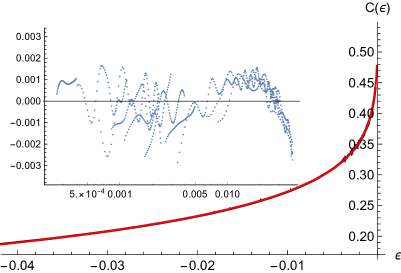
Figure 14: (Colour on-line) Asymptotic specific heat $\operatorname{\mathcal{C}}(\varepsilon)$ and a fitted curve $y$ of Eq. (14) (indistinguishable) versus $\varepsilon$. Inset shows relative error $(y-\operatorname{\mathcal{C}})/\operatorname{\mathcal{C}}$ versus $\ln(-\varepsilon)$.

VII.2 The low-temperature range

Repeating this exercise on the low-temperature side ($\varepsilon>0$) turns out to be somewhat more demanding. The data are more noisy and the curves have a richer behaviour, making it harder to tell where the asymptotic curve starts and ends for finite $L$. But, being a bit more restrictive in our choices, we can piece together the curves for $6\leq L\leq 160$ to obtain a rough limit curve for $0.149720\leq K\leq 0.2$, or, $0.00018\lesssim\varepsilon\leq 0.336$. The resulting limit curve and some finite examples are shown in Fig. 15.

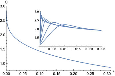
Figure 15: (Colour on-line) Asymptotic specific heat $\operatorname{\mathcal{C}}(\varepsilon)$ versus $\varepsilon$ for low temperatures. Inset shows $\operatorname{\mathcal{C}}_{L}$ versus $\varepsilon$ for $L=6$, $8$, $12$, $16$, $24$, $32$, $48$, $64$, $96$. Asymptotic curve $\operatorname{\mathcal{C}}_{\infty}$ built from piecing together $\operatorname{\mathcal{C}}_{L}$ for $6\leq L\leq 160$.

Fitting $y=A_{0}+A_{1}\varepsilon^{\theta^{+}}$ over different intervals works fine if we limit the data at an upper bound of $\varepsilon<0.015$. Adjusting the upper bound between $0.010$ and $0.015$ gives parameters $A_{0}=3.60(1)$, $A_{1}=-2.856(1)$ and $\theta^{+}=0.145(2)$ and we show $y$ and $\operatorname{\mathcal{C}}$ in Fig. 16. The relative error, shown in the inset, is larger here than for $\varepsilon<0$ but not by much.

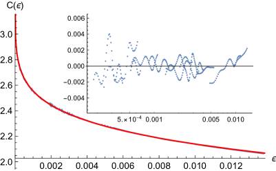
Figure 16: (Colour on-line) Asymptotic specific heat $\operatorname{\mathcal{C}}(\varepsilon)$ and the fitted curve $y=3.60-2.856\varepsilon^{0.145}$ (indistinguishable) versus $\varepsilon$. Inset shows relative error $(y-\operatorname{\mathcal{C}})/\operatorname{\mathcal{C}}$ versus $\ln(\varepsilon)$.

The fitted curve then suggests an upper bound of $3.60$. In Fig. 17 we show $3.60-\operatorname{\mathcal{C}}(\varepsilon))$ versus $\varepsilon$ in a log-log plot, again demonstrating the linear behaviour in such a plot.

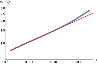
Figure 17: (Colour on-line) Log-log plot showing $3.60-\operatorname{\mathcal{C}}(\varepsilon)$ versus $\varepsilon$. The red line is $y=\ln(2.856)+0.145x$ where $x=\ln(\varepsilon)$.

Next we try the divergent scenario on the low-temperature side as well. Fitting the three term expression of Eq. (14) works quite well over a wide interval, whereas its two-term form fails to be convincing for all intervals. Over $\varepsilon<0.04$ (changing the upper bound to obtain error bars) we find $A_{0}=-1.85(2)$, $A_{1}=1.851(3)$ and $A_{2}=1.61(3)$. This is shown in Fig. 18 and the fit indeed appears convincing as the relative error shows.

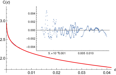
Figure 18: (Colour on-line) Asymptotic specific heat $\operatorname{\mathcal{C}}(\varepsilon)$ and an indistinguishable fitted curve $y$ of Eq. (14) (see text for details) versus $\varepsilon$. Inset shows relative error $(y-\operatorname{\mathcal{C}})/\operatorname{\mathcal{C}}$ versus $\ln(\varepsilon)$.

As we have seen, in the canonical ensemble both scenarios can give as plausible fits to the data. However, both here and in the section on finite-size scaling we consistently see cleaner fits for the mean-field scenario, means less trends in the residual errors. The bounded scenario also gives a simpler model for the data, while the divergent scenario requires three terms to work even with a modified the higher-order correction term.

VII.3 A comparison with higher dimensions

In Ref. [34] values for the two singular exponents $\theta^{-}$ and $\theta^{+}$ which we have used for the bounded scenario, as well as the limiting curves were found for larger dimensions. This was done via Monte Carlo data for dimensions 5, 6 and 7, and was derived exactly for the mean-field limit of the Ising model on complete graphs. Using data from that paper we show in Fig. 19 the suggested limit specific heat for systems dimensions 4, 5, 6, 7 and the mean-field case. The exact form used for $D=4$ is $\operatorname{\mathcal{C}}(\varepsilon)=3.60-2.86\varepsilon^{0.15}$ for $\varepsilon>0$, $\operatorname{\mathcal{C}}(\varepsilon)=0.81-0.86(-\varepsilon)^{0.10}$ for $\varepsilon<0$ and $\operatorname{\mathcal{C}}(0)=1.84$. As we can see, the behaviour for $D=4$ is consistent with those for higher dimensions

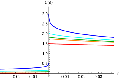
Figure 19: (Colour on-line) Asymptotic specific heat $\operatorname{\mathcal{C}}(\varepsilon)$ versus $\varepsilon$ for cases (downwards) 4D (blue), 5D (cyan), 6D (green), 7D (orange) and mean-field (red).

VII.4 Inside the scaling window

For $D\geq 5$ we know that the Ising model on the cyclic cubic lattice Ref. [35], just like the model on complete graphs Ref. [36], have several nested scaling windows, inside of which we see a non-trivial behaviour. Assuming that the model for $D=4$ follows the same pattern, having a bounded specific heat, we here attempt to reconstruct the limiting specific heat for one of these scaling windows, that given by taking $\kappa$ as the scaled energy.

In Fig. 20 we show the limit $\operatorname{\mathcal{C}}(\kappa)$ and the finite-$L$ $\operatorname{\mathcal{C}}_{L}(\kappa)$ versus $\kappa=L^{2}(K-K_{c})/K_{c}$. Here we use the estimate for the critical coupling $K_{c}=0.14969377$, but the overall picture does not change much when changing $K_{c}$ in the 8th decimal. The correction term from the maximum specific heat, $0.224/L^{2}$, translates to $\kappa^{*}=0.224/K_{c}\approx 1.49$. The asymptotic $\operatorname{\mathcal{C}}(\kappa)$ is obtained from fitting a line to $\operatorname{\mathcal{C}}_{L}(\kappa)$ versus $1/L^{1/5}$ for $L\geq 32$ giving a rough estimate of the limit, see Fig. 9. The location of the maximum of the limit $\operatorname{\mathcal{C}}(\kappa)$ curve almost matches the line obtained from the finite-size maxima. The maximum value of the limit curve is $C_{\max}=4.37$, located at $K=1.49$, and the limit at $\kappa=0$ is $\operatorname{\mathcal{C}}(0)=1.84$.

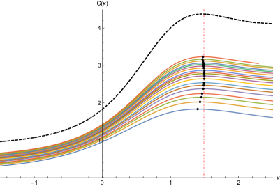
Figure 20: (Colour on-line) Limit specific heat $\operatorname{\mathcal{C}}(\kappa)$ (dashed) and $\operatorname{\mathcal{C}}_{L}(\kappa)$ for $L=6,8,\ldots,256$ (upwards). Dots mark location of maximum for $\operatorname{\mathcal{C}}_{L}$. Dot-dashed vertical line is $\kappa=1.49$ of Fig. 21.

VIII Scaling for critical points and the value of $K_{c}$

In this section we will examine additional finite-size critical points for the different energy moments and use them to better estimate the critical temperature $K_{c}$

VIII.1 The specific heat

In Fig. 21 we show the location of the maximum specific heat, $K_{c}(L)$, versus $1/L^{2}$ for $L\geq 64$. Fitting lines to different $L$-ranges with $24\leq L_{\min}\leq 64$ gives $K_{c}=0.14969372(13)$ where the error bar also matches the mean difference between the line and the points for $L\geq 64$. There are problems with estimating this maximum. It is a wide and not very distinct maximum and is thus sensitive to the slightest noise in the data. It is also comparatively far from $K_{c}$ and the scaling is rather slow (only $1/L^{2}$). Nevertheless, $1/L^{2}$ appears correct since there is no systematic correction for large $L$, see inset plot of Fig. 21.

It has been suggested that the location of such a pseudocritical point should approach $K_{c}$ as $L^{-2}(\ln L)^{-1/6}$ [32, 33] but we find no such indication here. In fact, we let Mathematica fit the points to an expression of the form $A_{0}+A_{1}L^{-2}+A_{2}L^{-2}(\ln L)^{-1/6}$ but depending on which points are included in such a fit the coefficient $A_{2}$ ends up being very close to zero. Fitting for example $L\geq 32$ and removing one point at a time to obtain an average and an error bar we find $A_{0}=0.14969372(5)$, $A_{1}=0.218(7)$ and $A_{2}=0.004(5)$ (error bar from standard deviation), that is, $A_{2}$ is effectively zero with an error bar comparable to its mean value. This also holds for other choices of $L$-ranges.

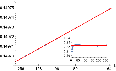
Figure 21: (Colour on-line) Location $K_{c}(L)$ of specific heat maximum versus $1/L^{2}$ for $L=64$, $80$, $96$, $112$, $128$, $160$, $192$, $256$. The fitted line is $y=0.14969372(13)+0.224x$ where $x=1/L^{2}$. The inset shows $(K_{c}(L)-K_{c})L^{2}$ versus $L$ and the constant line $y=0.224$.

The finite-size behaviour of the specific heat also provides a third, and more powerful, technique for estimating $K_{c}$, namely to use $(L,2L)$-crossing points of the specific heat. Let $K_{x}=K_{x}(L_{1},L_{2})$ denote the point where $\operatorname{\mathcal{C}}_{L_{1}}(K_{x})=\operatorname{\mathcal{C}}_{L_{2}}(K_{x})$. In general one could use $(L,bL)$ crossing points but since our data give the largest number of such pairs for $b=2$ we will only use these. In Fig. 22 we show an example of such a crossing point for the case $(128,256)$. An advantage of these points is that they are quite distinct and occur very close to $K_{c}$.

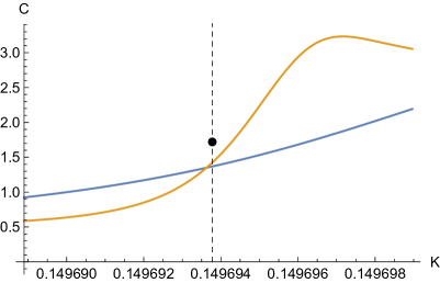
Figure 22: (Colour on-line) Specific heat $\operatorname{\mathcal{C}}_{L}(K)$ and $\operatorname{\mathcal{C}}_{2L}(K)$ (steeper) for $L=128$ indicating a distinct $(128,256)$ crossing point $K_{x}(128,256)=0.14969363$ close to $K_{c}$ (dashed line). The point is at an estimated limit of $\operatorname{\mathcal{C}}_{L}(K_{c})$ when $L\to\infty$.

In Fig. 23 we show $K_{x}(L,2L)$ for $32\leq L\leq 128$ and a fitted line giving $K_{x}=0.14969379(1)-0.0093(1)\,L^{-9/4}$. The error bars are, as before, obtained from fitting lines to $K_{x}$ versus $1/L^{9/4}$ for $L$-ranges with $24\leq L_{\min}\leq 64$ and taking the mean difference between a fitted line and the points for $L\geq 32$. In fact, this technique appears quite robust and does not depend strongly on which points are included in the fits. A huge benefit is that the correction term seems to be of order $1/L^{9/4}$ with negligible higher-order correction terms. Unfortunately we do not have a theoretical basis for this exponent. We think it is supported by looking at the correction $(K_{x}-K_{c})L^{9/4}$ which is almost constant $-0.0093$ for $L\geq 16$, see inset of Fig. 23. Alternatively we can express the rescaled crossing point as $\kappa_{x}\approx-0.062/L^{1/4}$ to clearer show that this point goes to zero also in the scaling window.

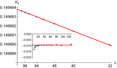
Figure 23: (Colour on-line) Specific heat crossing points $K_{x}(L,2L)$ versus $1/L^{9/4}$ for $L=32$, $40$, $48$, $56$, $64$, $80$, $96$, $112$ and $128$. The fitted line is $0.14969379-0.0093x$ where $x=1/L^{9/4}$. The inset shows the $(K_{x}-0.14969379)L^{9/4}$ and the line $y=0.0093$.

The value of $\operatorname{\mathcal{C}}_{L}(K_{x})$ scales very much like that of $\operatorname{\mathcal{C}}_{L}(K_{c})$ of Fig. 9. We estimate $\operatorname{\mathcal{C}}_{L}(K_{x})=1.838(2)-1.29(1)/L^{1/5}$ thus giving a slightly different correction term but approximately the same limit (not shown) though there is more noise here than for $\operatorname{\mathcal{C}}_{L}(K_{c})$.

VIII.2 Energy kurtosis

In Fig. 24 we show the energy (excess) kurtosis $\operatorname{\mathcal{G}}_{L}(\kappa)$ for all $L$. There is a distinct minimum near $\kappa=1$ and a maximum approaching from the left. Shortly we will estimate the scalings for these critical points.

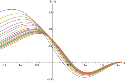
Figure 24: (Colour on-line) Excess kurtosis $\operatorname{\mathcal{G}}(\kappa)$ for $6\leq L\leq 256$.

We will, however, start with the value at $K_{c}$ as it turns out to be an excellent arbiter of $K_{c}$. In Fig. 25 we show $\operatorname{\mathcal{G}}_{L}(K_{c})$ versus $L$ with $K_{c}=0.149693785$ and also for $K_{c}\pm 5\times 10^{-8}$ where the points clearly trend up or down. In fact, this effect is distinctly visible already for $\pm 2\times 10^{-8}$ which means that we can set $K_{c}=0.149693785(20)$. This is in perfect agreement with the result in relation to Fig. 10. Obviously some noise sets in for $L=192,256$ but we have based the present $K_{c}$ on $L\leq 160$ giving very small fluctuations ($\pm 0.001$) around the line.

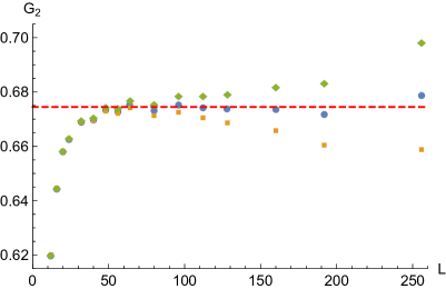
Figure 25: (Colour on-line) Kurtosis $\operatorname{\mathcal{G}}_{L}(K_{c}$ versus $L$ for $10\leq L\leq 256$ with $K_{c}=0.149693785$. The dashed constant line through the points is $y=0.674$ (fitted on $L\geq 48$). The points trending downwards and upwards are for $K_{c}\pm 5\times 10^{-8}$.

Let us now continue with the maxima and minima of Fig. 24. Let first $K_{c}(L)$ be the local minimum of $\operatorname{\mathcal{G}}_{L}$ located near $\kappa=1$. This minimum is quite distinct and we thus expect a good estimate of $K_{c}$. Indeed, fitting as before $K_{c}(L)=A_{0}+A_{1}/L^{2}$ to data ranges $L_{\min}\leq L\leq 256$ with $32\leq L_{\min}\leq 128$ we find $K_{c}=A_{0}=0.14969380(2)$ and $A_{1}=0.1579(4)$ (from median and interquartile range), a surprisingly sharp estimate of $K_{c}$ from this kind of critical point. Fitting instead $y=A_{0}+A_{1}/L^{a}$ does not change the result much. We then obtain $K_{c}=A_{0}=0.14969378(4)$, $A_{1}=0.156(9)$ and $a=2.00(1)$, quite consistent with the previous only with larger error bars. Note in particular the $a$-estimate, showing no sign of any logarithmic correction.

For the location $K_{c}(L)$ of the maximum we need a correction term. Fitting $K_{c}(L)=A_{0}+A_{1}/L^{2}+A_{2}/L^{a}$ to data ranges $20\leq L_{\min}\leq 64$ gives fairly stable results: $A_{0}=0.14969380(5)$, $A_{1}=-0.054(13)$, $A_{2}=-0.31(20)$ and $a=2.56(26)$. Fixing instead $a=2.5$ and repeating for $32\leq L_{\min}\leq 128$ we obtain $K_{c}=A_{0}=0.14969381(5)$, $A_{1}=-0.051(5)$ and $A_{2}=-0.27(5)$, consistent with the previous free-$a$ estimate. One might here consider using a correction term of the form $A_{2}L^{-2}(\ln L)^{-1/6}$ but the result then depends strongly on $L_{\min}$ with clear trends in the $A_{i}$. Using instead a free exponent $a$ of $\ln L$ gives too much noise in $a$ to say what its value is. This suggests that the data do not favor a correction on this form. In Fig. 26 we show $K_{c}(L)$ for both the maximum and the minimum and the fitted curves. In rescaled form they can now be expressed as $\kappa^{*}=1.055(3)$ and $\kappa^{*}=-0.34(3)-1.8(3)/\sqrt{L}$ for the minimum and maximum respectively.

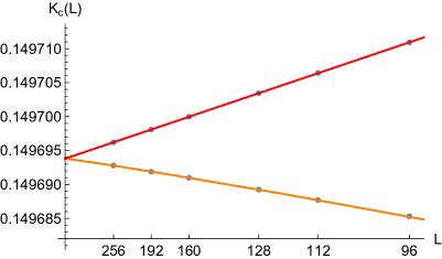
Figure 26: (Colour on-line) Location $K_{c}(L)$ of the maximum (from below) and minimum (from above) kurtosis versus $1/L^{2}$ for $L=96$, $112$, $128$, $160$, $192$, $256$. The red line is $y=0.14969380(2)+0.1579(3)x$ and the orange curve is $y=0.14969381(5)-0.051(5)x-0.27(5)x^{5/4}$, where $x=1/L^{2}$. See text for information on error bars.

We shall also attempt to estimate the scaling of the maximum and minimum values. First we need to find the correct leading order correction. Fitting $\operatorname{\mathcal{G}}=A_{0}+A_{1}/L^{a}$ to $32\leq L_{\min}\leq 64$ for the maxima gives $a=0.50(4)$ but for the minima we obtain $a=0.60(15)$. There is, however, more support for a leading order correction term $A_{1}/\sqrt{L}$.

Having selected $a=1/2$ we fit the two-term formula to the minima for $32\leq L_{\min}\leq 96$ and obtain $\operatorname{\mathcal{G}}_{\min}=-0.2817(5)-0.209(6)/\sqrt{L}$. For $L<32$ some correction term becomes necessary though but we do not know what form it should take. The same procedure applied to the maxima gives us $\operatorname{\mathcal{G}}_{\max}=0.764(1)+1.72(1)/\sqrt{L}$, again with higher-order corrections needed for $L<32$.

We shall end the subject of kurtosis by studying its $(L,2L)$-crossing point, denoted $K_{x}$. In Fig. 27 we show an example for $L=128$. What is striking with this crossing point is how extremely close it is to $K_{c}$. We find the very small difference $K_{x}-K_{c}\propto 1/L^{4}$. In Fig. 28 we show the crossing point $K_{x}$ versus $1/L^{4}$ for $L\geq 10$ and an inset for the larger $L$. Fitting $K_{x}=A_{0}+A_{1}/L^{4}$ for $10\leq L_{\min}\leq 56$ gives $K_{c}=A_{0}=0.149693775(15)$ and $A_{1}=0.17(4)$. The points appear more scattered for $L\geq 64$ but they stay within $\pm 2\times 10^{-8}$ from the line.

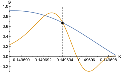
Figure 27: (Colour on-line) Kurtosis $\operatorname{\mathcal{G}}_{L}$ and $\operatorname{\mathcal{G}}_{2L}$ for $L=128$ indicating a distinct $(128,256)$ crossing point close to $K_{c}$ (dashed line). Here $K_{x}(128,256)=0.149693796$. The point is at the estimated limit of $\operatorname{\mathcal{G}}_{L}(K_{c})=0.675$ when $L\to\infty$.

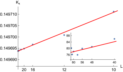
Figure 28: (Colour on-line) Kurtosis crossing point $K_{x}(L,2L)$ versus $1/L^{4}$ for $10\leq L\leq 128$. The red line is $y=0.149693775(15)+0.17(4)x$ where $x=1/L^{4}$. Inset shows $K_{x}$ for $L=40$, $48$, $56$, $64$, $80$, $96$, $128$ and the same line. The numbers on the $y$-axis are the decimals after $0.149693\ldots$.

VIII.3 Energy

We have obtained many estimates of $K_{c}$ of varying precision depending on the studied quantity and approach. The crossing point of the specific heat gave a sharp estimate of $K_{c}$. The energy kurtosis turned out to be extremely useful for pinning down $K_{c}$ from several different perspectives; local maxima and minima, crossing points, constant kurtosis for large $L$. On the other hand, the local maximum of the specific heat was less useful, giving comparatively wide error bars. Taking an intersection of all these estimates and using the smallest of the error bars we find $K_{c}=0.149693785(10)$. This also agrees with the recent [37] $K_{c}=0.14969388(22)$. Our old estimate [25] of $K_{c}=0.1496947(5)$ was then off by less than two of its error bars.

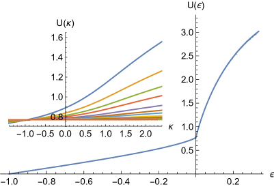
Figure 29: (Colour on-line) Asymptotic energy $\operatorname{\mathcal{U}}(\varepsilon)$ versus $\varepsilon$. Inset shows $\operatorname{\mathcal{U}}$ versus reduced coupling $\kappa$ for $6\leq L\leq 256$.

The asymptotic energy $\operatorname{\mathcal{U}}(\varepsilon)$, obtained exactly as we did above for the specific heat, is shown in Fig. 29. The inset shows the energy versus the rescaled coupling for a range of system sizes. Clearly their limit approaches some constant inside the scaling window. Fitting $y=A_{0}+A_{1}/L^{2}$ to a sequence of $\operatorname{\mathcal{U}}_{L}(\kappa)$ for a fixed $\kappa$ is of course one possibility. Unfortunately this requires higher order corrections and it is not clear what exponent a further term should use. Including a third term $A_{2}/L^{a}$ gives very unstable results at $\kappa=0$.

However, if we let $\kappa=-0.25$ then the higher-order corrections effectively vanish. In Fig. 30 we show $\operatorname{\mathcal{U}}_{L}(\kappa=-0.25)$ versus $1/L^{2}$ and the inset shows only noise-like corrections. The result is $\operatorname{\mathcal{U}}_{c}=A_{0}=0.7704434(10)$ and $A_{1}=2.730(2)$ where error bars indicate mean difference between line and points and standard deviation in fits over $20\leq L_{\min}\leq 96$, respectively.

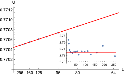
Figure 30: (Colour on-line) Energy $\operatorname{\mathcal{U}}_{L}(\kappa)$, where $\kappa=-0.25$, versus $1/L^{2}$ for $64\leq L\leq 256$. The red line is $y=0.7704434(10)+2.730(2)x$ (see text) with $x=1/L^{2}$. Inset shows $(\operatorname{\mathcal{U}}_{L}(\kappa)-0.7704434)L^{2}$ versus $L$ and the line $y=2.73$.

IX The Universality Class

After a full analysis of our data from both the microcanonical and canonical point of view we are now ready for the main question of this paper: Which universality class does the 4-dimensional Ising model belong to? The existing literature has actually considered three possibilities: mean-field behaviour with bounded specific heat, a logarithmic singularity in the specific heat of the type as in the $\phi^{4}$-model, or a weak first order phase transition.

As mentioned in the introduction, assuming that we have a $\phi^{4}$-singularity one is led to expect a very slow divergence, see Eq. (13) of the specific heat as a function of $L$, the term $(\ln L)^{1/3}$ merely increases from 1.4 to 1.9 when $L$ increases from 16 to 1024. Because of this one would not expect to clearly distinguish this case from one with bounded heat via classical Monte Carlo simulation. As we have seen in Sections VI and VII the data for the canonical ensemble can be fitted to the finite-size scaling and the asymptotic form expected from the $\phi^{4}$-case. However, for both scaling and asymptotics we get smaller errors when using the scaling and asymptotic forms given by the scenario with a bounded specific heat. So, as expected the difference is not clear, but a bounded specific heat consistently fares better.

However, when instead examining the model in the microcanonical ensemble the difference is clear cut. In Section V we found that for the full range of $L$ used here the minimum value of $\operatorname{K}^{\prime}(U)$ is positive and increasing to a finite, positive limit as a function of $L$. The only assumption underlying this conclusion is that the Ising model in dimension 4 does not have finite-size effects so large that lattices with $L\leq 256$ do not even present the right direction of change for $\operatorname{K}^{\prime}(U)$ as function of $L$, something which would be so far unheard of.

First, the fact that $\operatorname{K}^{\prime}$ is positive means that we have a positive specific heat. This in turn means that, unlike the situation in dimension 5 [5], we do not have a meta-stable region for finite $L$ and so a purely second order phase transition. Here we can conclude that the weak first-order phase transition suggested in [15, 16] is ruled out, even in the quasi-first order form found in [5]. In the thermodynamic limit a first-order phase transition is already ruled out by the rigorous results in [2, 3]. The indications for a first-order phase transition came from a numerical renormalisation group technique which involves both a finite lattice size $L$ and a cut-off parameter $D$. So, even if the method is sound this could indicate that the accuracy as a function of these two parameters is less than expected. This would also agree with the fact that the estimate for $K_{c}$ in [15] deviates noticeably from the currently best. The suggested first-order transition has been used in some works on the Higgs field [38, 39] which might instead be redone with a mean-field transition in mind.

Second, and more importantly the fact that the asymptotic value of $\operatorname{K}^{\prime}(U)$ is strictly positive means that we have a finite upper bound for the specific heat in the thermodynamic limit. This rules out a singularity of the same type as in the $\phi^{4}$-model, and of course any other form of divergent specific heat. In Section VII we saw that, just as for higher dimension, we could fit the canonical data well to a discontinuous specific heat curve with distinct left and right-side limits at $K_{c}$. The values we obtained there also agreed well with the bounds found in Section V for those limits, via the estimated values for $\operatorname{K}^{\prime}(U)$. Here we can also note that the limit values for the specific heat implies that the high- and low-$U$ limits for $\operatorname{K}^{\prime}(U)$ should be 0.0277 and 0.00622, which is compatible with the data in Fig. 5. If the model follows the behaviour seen in higher dimension [5] then one expects $\operatorname{K}^{\prime}(U)$ to approach these limit values controlled by a pair of high- and low-$U$ singular exponents, and we have found good fits of that form to our data.

Together this leads to the conclusion that the Ising model and the $\phi^{4}$-model do not belong to the same universality class. Instead, the first has a mean-field type bounded discontinuous jump in the specific heat at the critical point, and the second a logarithmically divergent specific heat at the same point.

Following the sometimes used terminology that the logarithmic singularity of the $\phi^{4}$-model is a ”correction” to mean field behaviour one could still claim that the two models belong to the same universality class, albeit with and without corrections. However, in our view this is not consistent with the generally accepted idea that universality classes correspond to fixed points of the renormalization group flow. Since renormalisation does detect the logarithmic singularity of the 2D Ising model the method should be sensitive to such singularities more generally, as long as one works with a large enough subspace for the flow. Hence one should expect separate fixed points for the $\phi^{4}$-model and a pure mean-field singularity. One might also simply think that calling the leading order part of the singularity in 4-dimensions a ”correction” appears inaccurate.

X Discussion

Our main conclusion here, that the Ising model and the $\phi^{4}$-model belong to distinct universality classes for $D=4$ will be surprising to some, but at the same time does not invalidate any major theoretical tools or methods from the physics literature. Rather, it enriches the picture since we now have two models which at their upper critical dimension have the same, mean-field, critical exponents but still have distinct lower order behaviour.

As mentioned in the introduction, having the same spatial dimension and symmetries is merely the simplest candidate for a list of properties defining a universality class. One of the major heuristic underpinnings for the existence of universality classes is the existence of fixed points for the renormalisation group flow on the space of models, or hamiltonians, and here a split into two universality classes would simply mean that there is some new variable which differentiates two distinct fixed points for this flow. Today we know [40] the renormalisation is a far more sensitive, and often precarious, procedure than the early works assumed and it would not be surprising if new features are relevant exactly at the upper critical dimension.

At the moment we cannot answer what this new differentiating variable corresponds to, but at a first glance there are two features which distinguish the Ising and $\phi^{4}$-model from each other. First, the cardinality of the single-spin state space differentiates the Ising model from the $\phi^{4}$-model for all finite parameters $(b,\lambda)$. Second, is the fact that the spin values in the $\phi^{4}$-model are unbounded, something which we alluded to already in the introduction in connection with how the $\phi^{4}$-model may be approximated by block-spins based on the Ising model. The $\phi^{4}$-model with spin values restricted to a fixed finite interval $(-a,a)$ might provide an interesting intermediate case which could rule out the first of these properties as the relevant one.

In this paper we have focused on energy related properties of the model, with emphasis on the specific heat, but in our sampling runs we have also collected data for the magnetisation. This has been done so that both the canonical and microcanonical magnetisation distributions can be reconstructed and we will provide an analysis for both $D=4$ and $D=5$ in an upcoming paper. That analysis will shed more light on the scaling limit of the Ising model and the related quantum field theory.