Yangian-invariant fishnet integrals in 2 dimensions as volumes of Calabi-Yau varieties

Abstract

We argue that $\ell$-loop Yangian-invariant fishnet integrals in 2 dimensions are connected to a family of Calabi-Yau $\ell$-folds. The value of the integral can be computed from the periods of the Calabi-Yau, while the Yangian generators provide its Picard-Fuchs differential ideal. Using mirror symmetry, we can identify the value of the integral as the quantum volume of the mirror Calabi-Yau. We find that, similar to what happens in string theory, for $\ell=1$ and 2 the value of the integral agrees with the classical volume of the mirror, but starting from $\ell=3$, the classical volume gets corrected by instanton contributions. We illustrate these claims on several examples, and we use them to provide for the first time results for 2- and 3-loop Yangian-invariant traintrack integrals in 2 dimensions for arbitrary external kinematics.

Multi-loop Feynman integrals are the cornerstone of all modern perturbative approaches to quantum field theory (QFT) and a backbone of precision computations for collider and gravitational wave experiments. It is therefore of utmost importance to have efficient ways for their computation and a solid understanding of the underlying mathematics. Over the last years, it has become clear that the mathematics relevant to Feynman integrals is tightly connected to certain topics in geometry. One of the earliest observations was that 1-loop Feynman integrals compute the volumes of certain polytopes in hyperbolic spaces Davydychev and Delbourgo (1998); Schnetz (2010); Mason and Skinner (2011); Spradlin and Volovich (2011); Bourjaily et al. (2020a). Here the most prominent example is the 1-loop 4-point function with massless propagators in 4 space-time dimensions:

$$\int\frac{\textrm{d}^{4}\xi}{i\pi^{2}}\,\prod_{i=1}^{4}\frac{1}{(\xi-\alpha_{i})^{2}}=-\frac{4}{\alpha_{13}^{2}\alpha_{24}^{2}}\,\frac{D(z)}{z-\bar{z}}$$ (1)

with $\alpha_{ij}=\alpha_{i}-\alpha_{j}$. This integral features a so-called (dual) conformal symmetry Drummond et al. (2007) (with conformal weight 1 for each external point), and the variable $z$ is connected to the cross ratio formed out of the 4 external points $\alpha_{i}$. The function $D(z)$ is the so-called Bloch-Wigner dilogarithm, which is known to compute the volume of a simplex in hyperbolic 3-space, see e.g. Zagier (2007):

$$D(z)=\textrm{Im}\big{[}\textrm{Li}_{2}(z)+\log|z|\,\log(1-z)\big{]}\,.$$ (2)

Notably, this result for the 4-point integral can be bootstrapped from scratch, using a Yangian extension of the (dual) conformal symmetry Loebbert et al. (2020a).

The interpretation of Feynman integrals as volumes is so far only understood at 1 loop. While there is substantial evidence that, at least in special QFTs, the integrands of Feynman integrals are related to certain volume forms for generalisations of polytopes (see, e.g., Arkani-Hamed and Trnka (2014); Arkani-Hamed et al. (2018); Salvatori (2019); Arkani-Hamed et al. (2019); Damgaard et al. (2021)), it is an open question if at higher loops the values after integration can be interpreted as volumes of geometric objects. If that was indeed the case, it would shed new light on the mathematical structure of perturbative QFT, and possibly lead the way towards novel methods for the computation of Feynman integrals. The main goal of this paper is to take first steps into this direction and to present for the first time an infinite class of higher-loop Feynman integrals whose values can indeed be interpreted as a volume.

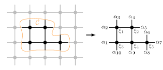
Figure 1: Ten-point five-loop fishnet integral cut out of a square tiling of the plane. If the $\ell=M\times N$ interior points span a rectangle, we denote the graph by $G_{M,N}$, with $M\leq N$.

I Fishnet integrals in 2 dimensions

In the remainder of this paper we focus on so-called fishnet integrals in 2 Euclidean dimensions, defined by a connected region cut out along a closed curve $\mathcal{C}$ intersecting the edges of a regular tiling of the plane by a square lattice (see Fig. 1 and Chicherin et al. (2018)). This defines a connected graph $G$ by considering only the edges of the lattice that intersect $\mathcal{C}$ (the external edges) or lie in its interior (the interior edges). Edges of $G$ connecting 2 vertices labeled by $a,b\in\mathbb{R}^{2}$ represent propagators $[(a-b)^{2}]^{-1/2}$, and we integrate over the positions of the internal vertices labeled $\xi_{i}$. It is well known that for a 2-dimensional QFT it is useful to consider complexified coordinates $a_{j}=\alpha_{j}^{1}+i\,\alpha_{j}^{2}$ and $x_{k}=\xi_{k}^{1}+i\,\xi_{k}^{2}$. The integrals we want to consider can then be written as

$$I_{G}(a)=\int\left(\prod_{j=1}^{\ell}\frac{\textrm{d}x_{j}\wedge\textrm{d}\bar{x}_{j}}{-2i}\right)\frac{1}{\sqrt{|P_{G}(x,a)|^{2}}}\,,$$ (3)

with $a=(a_{1},\ldots,a_{n})$, $x=(x_{1},\ldots,x_{\ell})$, and

$$P_{G}(x,a)=\Big{[}\prod_{i,j}(x_{i}-x_{j})\Big{]}\,\Big{[}\prod_{i,j}(x_{i}-a_{j})\Big{]}\,,$$ (4)

and the product ranges depend on the graph topology.

Every fishnet integral is invariant under the Yangian $Y(\mathfrak{so}(1,3))$ of the conformal group in 2 dimensions Chicherin et al. (2017); Loebbert et al. (2020b). The Yangian splits into holomorphic and anti-holomorphic parts:

$$Y(\mathfrak{so}(1,3))=Y(\mathfrak{sl}_{2}(\mathbb{R}))\oplus\overline{Y(\mathfrak{sl}_{2}(\mathbb{R}))}\,,$$ (5)

where the generators of $Y(\mathfrak{sl}_{2}(\mathbb{R}))$ act via partial differential operators on the holomorphic external points $a_{i}$ and annihilate the integral (at least for generic values of the external points). For the explicit form of the representation of the Yangian, we refer to Loebbert et al. (2020b). We note that invariance under the conformal subalgebra $\mathfrak{sl}_{2}(\mathbb{R})$ implies that we can write $I_{G}(a)=|F_{G}(a)|^{2}\,\phi_{G}(z)$, where $z=(z_{1},\ldots,z_{n-3})$ is a vector of conformal cross ratios formed out of the $a_{i}$ and $F_{G}(a)$ is a holomorphic algebraic function that carries the conformal weight.

Analytic results are known for various classes of fishnet integrals depending only on 4 external points, and consequently only on a single cross ratio, which we choose as $z=\operatorname{cr}(2,3,1,4)=a_{23}a_{14}/a_{21}a_{34}$. In Derkachov et al. (2019) analytic results are given for $G_{M,N}$, where the external points that are incident to the same side of the rectangle are identified (we call these graphs $G_{M,N}^{1}$) with determinants of (derivatives of) ladder graphs $G_{1,\ell}^{1}$. The ladder graphs $G_{1,\ell}^{1}$ themselves can be expressed as bilinear combinations of generalised hypergeometric functions. So far, no results are known for fishnet graphs in 2 dimensions depending on more than 1 cross ratio.

II 2D fishnets and Calabi-Yau geometries

We now argue that to every $\ell$-loop fishnet graph we can associate a CY $\ell$-fold. Loosely speaking, a CY $\ell$-fold is a complex $\ell$-dimensional Kähler manifold $M_{\ell}$ that admits a unique holomorphic $(\ell,0)$-form $\Omega$. This last condition can be phrased as follows: the cohomology groups $H^{r}(M_{\ell})$ admit a decomposition

$$H^{r}(M_{\ell})=\bigoplus_{p+q=r}H^{p,q}\,,$$ (6)

where the $H^{p,q}$ are generated by cohomology classes of $(p,q)$-forms, i.e., forms involving exactly $p$ holomorphic and $q$ anti-holomorphic differentials. The Hodge numbers of $M_{\ell}$ are $h^{p,q}=\dim H^{p,q}$. The CY condition then translates into $h^{\ell,0}=1$. Note that for a family of CY varieties parametrised by $d_{M}$ independent moduli, we have $h^{\ell-1,1}=d_{M}$ for $\ell\neq 2$. For K3 families $\ell=2d_{M}$ is the number of independent transcendental cycles minus two.

One possibility to define a family of CY $\ell$-folds is given by a double cover. Here we consider the constraint $y^{2}=P_{G}(x;a)$, double covering an $\ell$-dimensional projective base space $B$ with coordinate $x=(x_{1},\ldots,x_{\ell})$ and canonical class $K_{B}>0$. This defines a family $M_{G}$ parametrised by $a$ and with $(\ell,0)$-form

$$\Omega_{G}=\frac{\mu_{B}(x)}{\sqrt{P_{G}(x;a)}}\,,$$ (7)

where $\mu_{B}$ is the holomorphic measure on $B$. Note that $I_{G}$ is obtained by integrating $\Omega_{G}\wedge\overline{\Omega}_{G}$ over $\mathbb{C}^{\ell}$. To guarantee that we really obtain a family of CY $\ell$-folds, the degree of $P_{G}(x;a)$ has to be such that the canonical class vanishes. We consider $B=\bigtimes_{i=1}^{l}\mathbb{P}^{1}$ and $\mu_{B}=\wedge_{i=1}^{\ell}(x^{\prime}_{i}{\rm d}x_{i}-x_{i}{\rm d}x^{\prime}_{i})$ (with $[x_{i}:x^{\prime}_{i}]$ the homogeneous coordinate on the $i^{\textrm{th}}$ copy of $\mathbb{P}^{1}$), which is a natural compactification of the integration range $\mathbb{C}^{\ell}$ in (3). The vanishing of the canonical class then translates into the fact that $P_{G}(x;a)$ has to be of degree 4 in each $\mathbb{P}^{1}$. This condition is always fulfilled for fishnet graphs, because all internal vertices are 4-valent. For $\ell>1$, $M_{G}$ is typically a singular variety. Similar to Klemm et al. (2020), in all examples that we have studied (see below), these singularities can be resolved by deforming $M_{G}$ to a smooth CY $\ell$-fold, and we expect this to hold in all cases. We will further elaborate on this in Duhr et al. .

There is a natural set of integrals, called periods, that we can associate to a CY $\ell$-fold by integrating $\Omega_{G}$ over a basis of cycles $\Gamma_{i}$ that span the middle homology $H_{\ell}(M_{G},\mathbb{Z})$. The vector of periods is

$$\Pi_{G}=\Big{(}\int_{\Gamma_{1}}\!\!\!\Omega_{G},\ldots,\int_{\Gamma_{b_{\ell}}}\!\!\!\!\!\!\Omega_{G}\Big{)}\,,\,\,\,\,\,b_{\ell}=\dim H_{\ell}(M_{G},\mathbb{Z})\,.$$ (8)

The periods are multivalued functions of $a$. For every CY $\ell$-fold, there is a monodromy-invariant matrix $\Sigma$ that defines a bilinear pairing on the periods, and $\Sigma$ may be chosen symmetric for $\ell$ even and anti-symmetric (and even symplectic) for $\ell$ odd. It is well known how to relate the integral of $\Omega_{G}\wedge\overline{\Omega}_{G}$ to the monodomy-invariant combination of periods $\Pi_{G}^{\dagger}\Sigma\Pi_{G}$. This gives us a way to reduce the computation of fishnet integrals to the problem of finding the periods of $M_{G}$. The periods are solutions to certain differential equations, as we will now review.

The flatness of the Gauss-Manin connection implies the existence of an ideal of differential operators, called the Picard-Fuchs differential ideal (PFI), whose space of solutions is precisely spanned by the periods. The PFI can be derived by the Griffiths reduction method or a reduction of the Gel’fand-Kapranov-Zeleviskĭ system, see Klemm (2018) for a review. In practice, these methods can be rather slow, in particular in the case of many variables. We find that the PFI of $M_{G}$ contains the generators of $Y(\mathfrak{sl}_{2}(\mathbb{R}))$. Moreover, the group $\mathrm{Aut}(G)$ of automorphisms of $G$ acts on $Y(\mathfrak{sl}_{2}(\mathbb{R}))$ by permuting the external points $a_{i}$, and so the PFI naturally also contains these operators. Remarkably, in all cases we have studied, the complete PFI of $M_{G}$ is obtained in this way!

We can summarise our findings as follows.

Claim 1: For every $\ell$-loop fishnet graph $G$, there exists a family of CY $\ell$-folds $M_{G}$ with holomorphic $(\ell,0)$-form $\Omega_{G}$ such that $$\begin{split}I_{G}(a)&\,=(-i)^{\ell}\,\Pi^{\dagger}_{G}\,\Sigma\,\Pi_{G}\,,\end{split}$$ (9) and the PFI is generated by $\mathrm{Aut}(G)\cdot Y(\mathfrak{sl}_{2}(\mathbb{R}))$.

Let us make some comments about this result. First, Claim 1 implies that the periods of $M_{G}$ are Yangian invariants. The invariance under the conformal $\mathfrak{sl}_{2}(\mathbb{R})$ subalgebra implies that we can write $\Pi_{G}(a)=F_{G}(a)\widetilde{\Pi}_{G}(z)$, where $F_{G}(a)$ is a holomorphic and algebraic function of $a$. Second, we expect that the PFI has a point of maximal unipotent monodromy (MUM). For example for traintrack graphs $G_{1,\ell}$, we find that a MUM point can be identified as follows: we label an external point on a small side by $a_{1}$, and the others clockwise up to $a_{2\ell+2}$. Then a MUM point is at $z=0$, with $z_{k}=\operatorname{cr}(1,k+1,k+2,\ell+2)$, $z_{\ell}=\operatorname{cr}(1,\ell+1,2\ell+2,\ell+2)$ and $z_{\ell+k}=\operatorname{cr}(1,2\ell+3-k,2\ell+2-k,\ell+2)$ for $k=1,\ldots,\ell-1$. For the 1-parameter graphs $G_{M,N}^{1}$, we found MUM points up to $\ell=M\times N=12$ and a non-orientable graph, and we expect that they are present in full generality. Near the MUM-point $z=0$, there is a unique holomorphic period $\widetilde{\Pi}_{G,0}(z)$, that we can normalise to $\widetilde{\Pi}_{G,0}(z)=1+\mathcal{O}(z)$, and which multiplies the $d_{M}$ solutions linear in the logarithm, as well as the solution of maximal order $\ell+1$ in the logarithms. We define $\phi_{G}(z)=(-i)^{\ell}\,\widetilde{\Pi}^{\dagger}_{G}\,\Sigma\,\widetilde{\Pi}_{G}$. Finally, it is well known that $\widetilde{\Pi}_{G}^{\dagger}\,\Sigma\,\widetilde{\Pi}_{G}$ is proportional to $e^{-K(z,\bar{z})}$, where $K(z,\bar{z})$ is the Kähler potential for the Weil-Peterssen metric on the moduli space of $M_{G}$. This gives an interpretation of the Feynman integral in terms of the geometry. In the next section, we relate it to the quantum volume of the mirror.

We have verified that we can reproduce the complete PFI from the Yangian generators for $G_{1,2}$, $G_{1,3}$ and $G_{2,2}$. Having at our disposal the PFI of $M_{G}$, we can solve the differential equations satisfied by the periods using standard techniques in terms of series expansions Ince (1944). This basis of solutions, however, will in general be a linear combination with complex coefficients of the periods in (8). With the methods described in Bönisch et al. (2021a, b), it is possible to construct the change of basis and to find the monodromy invariant bilinear pairing $\Sigma$, and thus to compute $I_{G}(a)$ through (9). We have done this explicitly for $G_{1,2}$ and $G_{1,3}$. We have checked that our results numerically agree with a direct evaluation of the Feynman parameter representation for $I_{G}(a)$ for various values of $a$, and we find very good agreement (see Fig. 2). More details about the structure and the properties of the solutions will be provided in Duhr et al. .

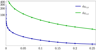
Figure 2: The functions $\phi_{G_{1,2}}(z_{1},z_{2},z_{3})$ and $\phi_{G_{1,3}}(z_{1},\ldots,z_{5})$ evaluated on the 1-dimensional slice $(z_{1},z_{2},z_{3})=\tfrac{s}{16}(1,2,3)$ and $(z_{1},\ldots,z_{5})=\tfrac{s}{16}(1,2,12,4,5)$ (for the definition of our cross ratios, see the main text). The continuous lines represent the results obtained from our analytic result in terms of CY periods, while the dots are obtained from a numerical evaluation of the Feynman parameter representation of $G_{1,\ell}$.

Let us conclude by commenting on the structure of the 4-point ladder graphs $G_{1,\ell}^{1}$ of Derkachov et al. (2019); Corcoran et al. (2022). At $\ell$ loops we have a 1-parameter family of CY $\ell$-folds whose PFI is generated by a single operator $L_{\ell}$ of degree $\ell+1$ that has a MUM-point at $z=0$, and we have $h^{p,\ell-p}_{\textrm{hor.}}=1$, $0\leq p\leq\ell$. These operators are special instances of the Calabi-Yau operators considered in Bogner (2013); van Straten (2018). We have checked up to $\ell=5$ that we reproduce the results of Derkachov et al. (2019) from our (9). For $\ell=1$, we obtain the Legendre family of elliptic curves, and the periods can be expressed in terms of elliptic integrals Derkachov et al. (2019); Corcoran et al. (2022):

$$\begin{split}\phi_{G_{1,1}^{1}}\!(z)&\,=\frac{4}{\pi^{2}}\,(\operatorname{K}\,\overline{\operatorname{K}}^{\prime}+\overline{\operatorname{K}}\,\operatorname{K}^{\prime})=\frac{8}{\pi^{2}}\,|\operatorname{K}|^{2}\,\textrm{Im}\,\tau_{1}\,,\end{split}$$ (10)

and $F_{G_{1,1}^{1}}\!(a)=\pi/\sqrt{a_{12}a_{34}}$. Here $\operatorname{K}\equiv\operatorname{K}(z)$ is the complete elliptic integral of the first kind and $\operatorname{K}^{\prime}\equiv\operatorname{K}(1-z)$, and we defined $\tau_{1}=i\operatorname{K}^{\prime}/\operatorname{K}$. For $\ell=2$, we obtain a 1-parameter family of K3 surfaces. It is known that every CY operator of degree 3 is equivalent to the symmetric square of a CY operator of degree 2 Doran (2000); Bogner (2013), and so we can express $G_{1,2}^{1}$ in terms of elliptic integrals. We define $\operatorname{K}_{\pm}=\operatorname{K}\big{(}\frac{1}{2}(1\pm\sqrt{1-z})\big{)}$ such that $(\operatorname{K}_{-}^{2},\operatorname{K}_{-}\operatorname{K}_{+},\operatorname{K}_{+}^{2})$ span the solution space of $L_{3}$. $G_{1,2}^{1}$ is then given by:

$$\phi_{G_{1,2}^{1}}\!(z) =\frac{2}{\pi^{4}}(\operatorname{K}_{+}\overline{\operatorname{K}}{}_{-}+\operatorname{K}_{-}\overline{\operatorname{K}}{}_{+})^{2}$$ (11)

$$=\frac{8}{\pi^{4}}\,|\operatorname{K}_{-}|^{4}(\textrm{Im}\,\tau_{2})^{2}\,,$$

with $\tau_{2}=i\operatorname{K}_{+}/\operatorname{K}_{-}$ and $F_{G_{1,2}^{1}}\!(a)\!=\!4\sqrt{2}\pi^{2}/\sqrt{a_{12}a_{34}a_{24}}$. For $\ell>2$, it is not possible anymore to express the periods of $M_{G_{1,\ell}^{1}}$ in terms of elliptic integrals.

III Fishnets as quantum volumes

The results of the previous section allow us to reduce the computation of $I_{G}(a)$ to the computation of the periods of $M_{G}$. Since (1) computes the volume of a hyperbolic simplex, it is natural to ask if we can interpret $I_{G}(a)$ as a volume of sorts. At this point, however, we face an issue. In (1) the ambient hyperbolic space of the simplex provides the canonical metric w.r.t. which the volume is computed. On $M_{G}$, however, we do not have any distinguished metric. Indeed, while $a$ fixes $\Omega_{G}$, and thus the complex structure, there is still substantial freedom to define a Kähler form, and thus a metric, on $M_{G}$. We now argue that we obtain a volume interpretation using mirror symmetry.

Mirror symmetry expresses the remarkable fact that CY $\ell$-folds come in pairs $(M_{G},W_{G})$ such that the cohomology groups $H^{p,q}(M_{G})$ and $H^{\ell-p,q}(W_{G})$ are exchanged. In particular, mirror symmetry exchanges the complex structures encoded in $H^{\ell-1,1}(M_{G})$ with the Kähler structures from $H^{1,1}(W_{G})$. Since $G$ defines via $\Omega_{G}$ a complex structure on $M_{G}$, mirror symmetry provides a Kähler form $\omega_{G}\in H^{1,1}(W_{G})$. Choosing $z$ such that $M_{G}$ has a MUM-point at $z=0$, we have

$$\omega_{G}=\sum_{i}t_{G,i}^{\mathbb{R}}(z)\,\omega^{(i)}\,,$$ (12)

where $\omega^{(i)}$ is a basis of $H^{1,1}(W_{G})$, and the $t_{i}^{\mathbb{R}}(z)=\textrm{Im}\,t_{i}(z)$ are given by the mirror map

$$t_{G,i}(z)=\widetilde{\Pi}_{G,i}(z)/\widetilde{\Pi}_{G,0}(z)\,,\quad i=1,\ldots,d_{M}\,,$$ (13)

where the $\widetilde{\Pi}_{G,i}(z)$ diverge like a single power of a logarithm at the MUM-point. The Kähler form, in turn, can be used to define a volume form $\omega_{G}^{\ell}/\ell!$ on $W_{G}$, and we can define the classical volume of $W_{G}$ as

$$\begin{split}\textrm{Vol}_{\textrm{cl}}(W_{G})&\,=\int_{W_{G}}\frac{\omega_{G}^{\ell}}{\ell!}\\ &\,=\frac{1}{\ell!}\sum_{i_{1},\cdots,i_{\ell}}C^{\textrm{cl}}_{i_{1},\cdots,i_{\ell}}\,t_{i_{1}}^{\mathbb{R}}(z)\cdots t_{i_{\ell}}^{\mathbb{R}}(z)\,,\end{split}$$ (14)

where the $C^{\textrm{cl}}_{i_{1},\cdots,i_{\ell}}$ are explicitly-computable integers, namely the (classical) intersection numbers of $M_{G}$.

Let us illustrate this on the examples of the ladder graphs considered at the end of the previous section. At 1 loop, we find $\textrm{Vol}_{\textrm{cl}}(W_{G_{1,1}^{1}})=t_{G_{1,1}^{1},1}^{\mathbb{R}}(z)=\textrm{Im}\,\tau_{1}$, which is the area of the fundamental parallelogram (with sides $(1,\tau_{1})$) that defines the elliptic curve $W_{G_{1,1}^{1}}$ associated to $G_{1,1}^{1}$. Similarly, we have $\textrm{Vol}_{\textrm{cl}}(W_{G_{1,2}^{1}})=\frac{1}{2}t_{G_{1,2}^{1},1}^{\mathbb{R}}(z)^{2}=\frac{1}{2}(\textrm{Im}\,\tau_{2})^{2}$. Comparing this to (10) and (11), we see that

$$\begin{split}\phi_{G_{1,1}^{1}}(z)&\,=\frac{4}{\pi^{2}}\,|\operatorname{K}|^{2}\,\textrm{Vol}_{\textrm{cl}}(W_{G_{1,1}^{1}})\,,\\ \phi_{G_{1,2}^{1}}(z)&\,=\frac{16}{\pi^{4}}\,|\operatorname{K}_{-}|^{4}\,\textrm{Vol}_{\textrm{cl}}(W_{G_{1,2}^{1}})\,,\end{split}$$ (15)

i.e., we see that the 1- and 2-loop ladder integrals are proportional to the classical volume of the mirror CY (the prefactor proportional to $\widetilde{\Pi}_{G_{1,\ell}^{1},0}$ defines the overall scale). We checked that the same statement holds for the 2-loop traintrack integral $G_{1,2}$, which depends on 3 independent cross ratios. However, starting from 3 loops, the last factor in (15) is no longer proportional to $\textrm{Vol}_{\textrm{cl}}(W_{G})$. This is not surprising: it is well known from string theory and mirror symmetry that for $\ell>2$ volumes of CY $\ell$-folds receive instanton corrections of order $e^{-t_{i}^{\mathbb{R}}}$. Their contribution is included in the quantum volume of $W_{G}$,

Claim 2: $\phi_{G}(z)$ is determined by the quantum volume of the mirror $W_{G}$ to $M_{G}$: $$\phi_{G}(z)=|\widetilde{\Pi}_{G,0}(z)|^{2}\,\textrm{Vol}_{\textrm{q}}(W_{G})\,.$$ (16)

Note that one could impose the following requirements on the quantum volume: i) It is real and positive; ii) it approaches in the limit $z_{i}\rightarrow 0$ (or equivalently in the large volume limit $t_{i}^{\mathbb{R}}\rightarrow\infty$) the classical volume (14); iii) it is monodromy-invariant, i.e., it uniquely extends over the complex moduli space. In (16), $\textrm{Vol}_{\textrm{q}}(W_{G})$ fulfils i) and ii) but not iii). Because of the normalisation of $\widetilde{\Pi}_{G,0}(z)=1+{\cal O}(z)$ one could define $\phi_{G}$ itself as the quantum volume, fulfilling i)-iii). Nevertheless $\textrm{Vol}_{\textrm{q}}(W_{G})$ seems the more canonical generalisation of the likewise not monodromy-invariant classical volumes in (15). Its CY 3-fold version also features in the analysis of non-perturbative properties of string compactifications in Lee et al. (2022).

We have checked Claim 2 on our examples for multi-loop traintrack integrals, as well as for the 1-parameter rectangular fishnet integrals of Derkachov et al. (2019). Claim 2 shows that it is possible to give a volume interpretation to all Yangian-invariant fishnet graphs. This extends the volume interpretation of (1) from 4 to 2 dimensions, but with the advantage that the interpretation naturally extends to higher loops. To our knowledge, this is the first time that multi-loop Feynman integrals were identified that compute volumes of geometric objects.

IV Conclusion

In this letter we have studied a class of Feynman integrals that connect research in mathematics, scattering amplitudes and integrability. Our main result is that Yangian-invariant $\ell$-loop fishnet integrals in 2 dimensions are naturally associated to families of CY $\ell$-folds and that the values of these integrals represent the quantum volume of the mirror CY. Indeed, we find that for $\ell\leq 2$, the traintrack integrals compute the classical volume of the mirror, in agreement with the fact that there are no instanton corrections for elliptic curves or K3 surfaces. Starting from $\ell=3$, instanton corrections can no longer be neglected. This is the first time that it was possible to identify a higher-loop Feynman integral as a volume of a geometric object. Intriguingly, we find that mirror symmetry plays an important role in this context.

Our results are not just of formal interest. Indeed, we find that we can reduce the problem of computing fishnet integrals in 2 dimensions to the geometrical question of finding the periods of $M_{G}$. Remarkably, solving this geometrical question receives input from physics, because we find that the Picard-Fuchs differential ideal is determined by the Yangian generators for fishnet graphs (and permutations thereof). We have illustrated this by providing for the first time results for 2-dimensional traintrack integrals at 2 and 3 loops.

Our work opens up several new directions for research, both in mathematics and in physics. First, it would be very interesting to study the geometrical properties of the CY varieties we have encountered in detail, in order to understand what role Yangian symmetry plays from the geometrical point of view. It is well known that 1-parameter families of CYs in various dimensions can be related by Hadamard-, symmetric- or anti-symmetric products van Straten (2018). As an example for the last relation we find that the solution space of the 4-point $G_{M,N}^{1}$ graphs is spanned, possibly up to rational functions Duhr et al. , by $M\times M$ sub-determinants of the Wronskian of the solutions of the $G_{1,M+N-1}^{1}$ graphs. These determinant relations are reminiscent of Basso-Dixon formulæ Basso and Dixon (2017); Derkachov et al. (2019), but relate integrals of different loop order. From the physics perspective, it would be interesting to clarify the role of the CY geometry in the context of the integrable fishnet theories defined in Gürdoğan and Kazakov (2016); Kazakov and Olivucci (2018), and in how far the CY geometry, and in particular the instanton corrections for $\ell>2$, play a role in the integrability of the theory. Finally, it would be important to clarify if a similar volume interpretation can also be achieved for other classes of multiloop Feynman integrals, including integrals in 4 space-time dimensions. The most natural place to start is to consider rectangular 4-point fishnet integrals in 4 dimensions, for which analytic results in terms of polylogarithms are known Usyukina and Davydychev (1993a, b); Basso and Dixon (2017). Recently, it was shown that $\ell$-loop Yangian-invariant traintrack integrals in 4 dimensions are related to CY $(\ell-1)$-folds Bourjaily et al. (2018a, b, 2019, 2020b); Vergu and Volk (2020) (and at 2 loops complete analytic results are known Ananthanarayan et al. (2020); Kristensson et al. (2021); Wilhelm and Zhang (2022)). It would thus be interesting to investigate if also in this case it is possible to identify a volume description via mirror symmetry.