GGI Lectures on Entropy, Operator Algebras and Black Holes

Abstract

These are slightly extended notes for my lectures at the workshop “Reconstructing the Gravitational Hologram” held at Galileo-Galilei Institute, Florence in June 2022.

1 Hawking, Unruh, Bisognano-Wichmann

The aim of these notes is to outline some interesting recent and not so recent developments at the interface between high energy physics and gravity, involving directly or indirectly ideas about entropy and quantum information. Emphasis is in particular on the connection to operator algebras. I am aware that operator algebras are fairly unfamiliar territory for most practitioners in high energy physics and quantum information, so my exposition will be quite informal for the most part, drawing attention to some methods and notions that I believe can be useful also for someone with only a casual interest in the technicalities of the subject. Before I begin let me emphasize that notions related to entropy have been used by mathematicians working in operator algebras almost from the beginning. These lectures by no means represent an exhaustive exposé of all these highly non-trivial connections. As these were covered by other excellent lectures at the workshop and there is an abundant literature, I also will not cover path integral approaches to entropies in QFT and quantum gravity, which can give very elegant and suggestive replica-trick representation of many quantities related to entanglement entropies.

Let me start, then, with the quintessential picture of Special Relativity ($x^{\pm}=x^{1}\pm x^{0}$) representing a Lorentz boost,

$$\begin{split}x^{0}(\tau)=&\cosh(a\tau)x^{0}+\sinh(a\tau)x^{1}\\ x^{1}(\tau)=&\sinh(a\tau)x^{0}+\cosh(a\tau)x^{1}.\end{split}$$ (1)

I am using units where the speed of light is $c=1$, so $a$ can be thought of as an acceleration parameter. Let

$$\beta=\frac{2\pi}{a}$$ (2)

By the addition theorem for $\sinh$ and $\cosh$:

$$\begin{split}x^{0}(\tau+i\beta)=&x^{0}(\tau)\\ x^{1}(\tau+i\beta)=&x^{1}(\tau).\end{split}$$ (3)

This suggests that vacuum state correlation functions of a quantum field $\phi$ should be periodic when expressed in terms of $\tau$, provided that their analytic continuation in $\tau$ makes sense. It turns out that this is the case precisely if we restrict to one of the wedges where the boost time has a definite direction, say the right wedge $\pm x^{\pm}>0$. You are invited to check this in the following exercise.

Exercise 1: Check that the imaginary part of the vector $(x^{0}(\tau+i\sigma),x^{1}(\tau+i\sigma),z^{A})$ is in the future lightcone for $0<\sigma<\beta$ if $(x^{0},x^{1},z^{A})$ is in the right wedge. Here $z^{A}$ are the coordinates along the edge of the wedge. In a quantum field theory (QFT) with vacuum vector $|\Omega\rangle$, it is usually assumed that the generator $P^{\mu}$ of spacetime translations has spectrum in the forward light cone and $P^{\mu}|\Omega\rangle=0$. By considering a suitable matrix element of $e^{iaP}$ and using the Heisenberg equation $e^{iaP}\phi(x)e^{-iaP}=\phi(x+a)$, show that the correlation function $\langle\Omega|\phi(x)\phi(x^{\prime})|\Omega\rangle$ has an analytic continuation $x^{\prime}\to x^{\prime}+iy^{\prime}$ and $x\to x+iy$ provided that $y^{\prime}$ is in the future- and $y$ is in the past lightcone.

Thus in the right wedge the correlation function of a Minkowski QFT has the following periodicity in imaginary boost time $\tau$:

$$\langle\Omega|\phi(\tau)\phi(\tau^{\prime}+i\beta-i0)|\Omega\rangle=\langle\Omega|\phi(\tau^{\prime}-i0)\phi(\tau)|\Omega\rangle.$$ (4)

The order of the operators has changed because we approach the real $x^{0}$-axis from above resp. below on the left resp. right sides of this equation – you can check this by being careful about the “$i0$”-prescriptions in these correlators. I have omitted the coordinates other than the boost time $\tau$ for easier readability. These other coordinates are to be held fixed.

It is important to note that we would get the same periodicity – also called the KMS condition – if we had for $x,x^{\prime}$ in the right wedge $W$

$${}_{W^{\prime}W}\langle\Omega|\phi(x)\phi(x^{\prime})|\Omega\rangle_{W^{\prime}W}\,\propto\,\operatorname{Tr}_{W}\phi(x)\phi(x^{\prime})e^{-\beta K}$$ (5)

where $K$ is the generator of boosts in the right wedge $W$, and where $W^{\prime}$ is the causal complement of the right wedge, i.e. the left wedge.

Here, I have formally assumed that

$${\mathscr{H}}={\mathscr{H}}_{W^{\prime}}\otimes{\mathscr{H}}_{W},\quad\text{(formal)}$$ (6)

because the wedge $W$ and the opposite wedge $W^{\prime}$ are causally disjoint, and to emphasize that this is a vector of the full Hilbert space, $|\Omega\rangle_{W^{\prime}W}$ is indexed by the union $W^{\prime}W$ of both wedges, the causal closure of which is the full spacetime. Also, formally, the generator of boosts in the right wedge ($x^{1}>0$) is:

$$K=\int_{{\color[rgb]{1,0,0}x^{0}=0,x^{1}>0}}x^{+}\Theta_{+}{}^{0}-x^{-}\Theta_{-}{}^{0}$$ (7)

where $\Theta_{\mu}{}^{\nu}$ is the stress energy tensor of the QFT. The conclusion of this reasoning is:

Unruh-Hawking: To an observer moving with constant acceleration $a$, the vacuum state looks thermal with Unruh-Hawking temperature

$$T=\frac{a}{2\pi}.$$ (8)

The thermal quanta can be harvested by coupling the quantum field to a so-called Unruh-DeWitt detector moving on the uniformly accelerated trajectory. If the detector represents a BBQ party on a rocket, then the sausages get cooked provided $a$ is sufficiently high. You do not want to to be a guest at this party of course because you would get cooked, too.

The above argument (with an important technical caveat regarding the status of the “density matrix” $e^{-\beta K}$ and the factorization of $\mathscr{H}$ into $\mathscr{H}_{W}\otimes\mathscr{H}_{W^{\prime}}$) as presented is essentially due to Bisognano and Wichmann [1], who however did not themselves make the connection with the Unruh effect. Instead, their motivation was to establish a technical property of the observable algebras ${{\cal A}}_{W}$ associated with the right wedge called “Haag duality” which I will explain later.

Almost literally the same reasoning applies to a Schwarzschild black hole

$$ds^{2}=-fd\tau^{2}+f^{-1}dr^{2}+r^{2}d\Omega^{2},\quad f=1-\frac{2MG}{r}.$$ (9)

Now the right wedge is the exterior of the black hole $r>r_{0}=2MG$ (outside the Schwarzschild radius $r_{0}$). The boosts correspond to shifts in $\tau$. The full picture is best constructed using Kruskal-Szekeres coordinates which are analogous to $x^{\pm}$.

An observer just hovering along the event horizon $H^{+}$ (or $H^{-}$) given by $r=r_{0}$ must be accelerated with

$$a=\frac{MG}{r_{0}^{2}}$$ (10)

which is an expression of Newton’s law.

By contrast to the Unruh effect where $a$ is a property of the observer, $a$ in the present context (also called the “surface gravity”) is fixed by requiring that the $\tau$-coordinate be normalized so that

$$ds^{2}\sim-d\tau^{2}+dr^{2}+r^{2}d\Omega^{2}\quad\text{as $r\to\infty$,}$$ (11)

so $\tau$ becomes the usual inertial time $x^{0}$ near infinity, due to gravitational redshift. Thus, unlike in the Unruh effect, in the black hole case, $a$ can be thought of as an intrinsic property of the spacetime. Nevertheless, either in the black hole case or the wedge, we can formally summarize the situation by saying that the reduced density matrix for the right wedge $W$ is

$$\omega_{W}=\operatorname{Tr}_{W^{\prime}}|\Omega\rangle\langle\Omega|\,\propto\,e^{-\beta K},$$ (12)

with $\beta=2\pi/a$ the inverse Hawking-temperature and with trace taken over the opposite wedge $W^{\prime}$. According to the 2nd law of black hole thermodynamics, the entropy of the black hole alone is given by

$$S=\frac{{\rm horizon\,area}}{4G}\qquad$$ (13)

in units where $k_{B}=\hbar=c=1$ with $4\pi r_{0}^{2}$ the area of the event horizon. This begs the question whether the entropy associated with $\omega_{W}$ (for all quantum fields including e.g. gravitions) could perhaps be equal to the area of the event horizon. This naive expectation turns out to be false as stated but is, as I hope to convince you, nevertheless a fruitful starting point for some considerations.

2 Entropy and relative entropy

The surprise we experience at seeing an event is greater if we thought that it was less likely. Thinking about our surprise at seeing two independent events such as winning the lottery twice, it is plausible that our surprise should in this case be additive, not multiplicative. Thus, the surprise at seeing an event whose probability we think is $p$ should be proportional to $\operatorname{ln}\frac{1}{p}$. Hence the average surprise experienced if events are distributed according to a probability distribution $\{p_{i}\}$ is

$$S(p)=\langle{\rm surprise}\rangle=\langle\operatorname{ln}\frac{1}{p_{i}}\rangle=-\sum_{i}p_{i}\operatorname{ln}p_{i}.$$ (14)

$S$ is of course the von Neumann entropy. In a finite quantum system, we can diagonalize the quantum density matrix as in $\rho=\sum p_{i}|i\rangle\langle i|$ and then $S(\rho)$ is given by exactly the same formula or equivalently by

$$S(\rho)=-\operatorname{Tr}\rho\operatorname{ln}\rho.$$ (15)

It frequently happens that our belief about the probability distribution for some events is different from the true probability distribution e.g. we believe a die is fair but it actually isn’t. Suppose we believe the distribution is $\{q_{i}\}$ but it really is $\{p_{i}\}$. The difference between our average surprise and the actual average surprise is

$$S(p|q)=\langle{\rm our\,surprise}\rangle-\langle{\rm actual\,surprise}\rangle=\langle\operatorname{ln}\frac{1}{q_{i}}\rangle-\langle\operatorname{ln}\frac{1}{p_{i}}\rangle=\sum_{i}p_{i}\operatorname{ln}\frac{p_{i}}{q_{i}}.$$ (16)

$S(p|q)$ is called the relative entropy. It can be seen as the information gained if we believed the distribution was $\{q_{i}\}$ but now we learn it is $\{p_{i}\}$ and is thus a measure of distinguishability between the two distributions. It is not symmetric in the two probability distributions as is psychologically plausible if we consider our surprise ($S(p|q)=\operatorname{ln}2$) at learning that the probability distribution for a the events ‘head’ and ‘tail’ of a coin actually is totally unfair $\{0,1\}$ when we believed the coin toss to be fair $\{\frac{1}{2},\frac{1}{2}\}$ versus our surprise ($S(p|q)=\infty$) at learning it is fair when we believed it to be totally unfair. Indeed, in the first case, we must see in $n$ drawings the events ‘tail’ $n$ times. Since we believe the coin is fair we ascribe a low but finite probability of $2^{-n}$ to this which never becomes zero, whereas in the opposite case any occurrence of ‘head’ will instantly destroy our belief that the probability distribution was $\{0,1\}$.

More formally, let $\{p_{\rm head},p_{\rm tail}\}$ and $\{q_{\rm head},q_{\rm tail}\}$ be two probability distributions and

$$\begin{split}C_{p}=&\bigg{\{}(i_{1},\dots,i_{n})\in\{{\rm head,tail}\}^{n}\,:\,\text{relative occurrence of head / tail is}\\ &\text{$=p_{\rm head}$ / $=p_{\rm tail}$ within small tolerance}\bigg{\}}.\end{split}$$ (17)

$C_{p}$ is a subset of $\{{\rm head,tail}\}^{n}$ to which an incorrect belief $\{q_{\rm head},q_{\rm tail}\}$ would assign a very small probability whereas it actually has probability tending to one for large $n$ and tolerance going to zero. Indeed, one can show

$${\rm Prob}_{q}(C_{p})\sim e^{-nS(p|q)}$$ (18)

for asymptotically large $n$ and small tolerance, which gives another interpretation of $S(p|q)$.

Exercise 2: Using that $-\operatorname{ln}$ is a convex function, derive Klein’s inequality $S(p|q)\geq 0$.

Contrary to the ordinary von Neumann entropy, there isn’t a unique generalization of the relative entropy for two non-commuting density matrices $\rho,\sigma$. Some possibilities are:

• Araki-Umegaki: $S_{AU}(\rho|~\sigma)=\operatorname{Tr}\rho\operatorname{ln}\rho-\operatorname{Tr}\rho\operatorname{ln}\sigma$.

• Measured: For an ONB $|i\rangle$, the transition amplitudes $p_{i}=\langle i|\rho|i\rangle,q_{i}=\langle i|\sigma|i\rangle$ give probability distributions. We can define

  $$S_{M}(\rho|\sigma)=\max_{{\rm ONBs}\,\{|i\rangle\}}S(p|q),$$ (19)

  which is called the measured relative entropy since we can think of $|i\rangle$ as the eigenvectors of some observable to be measured.

• Belavkin-Staszewski: $S_{BS}(\rho|\sigma)=-\operatorname{Tr}\rho\operatorname{ln}(\sqrt{\rho}^{-1}\sigma\sqrt{\rho}^{-1})$.

These are by no means the only possibilities. What separates a good generalization from a bad one is the satisfaction of an important inequality called the “Data Processing Inequality” (see below) and the existence of an operational meaning. An operational meaning is roughly a quantum information theoretic protocol for solving a problem for which the corresponding relative entropy gives the asymptotic rate of success. The Araki-Umegaki entropy passes both benchmarks, whereas the measured relative entropy does not satisfy the DPI and no straightforward operational meaning for the Belavkin-Staszewski entropy seems to be known. Therefore, in the following, I will restrict attention to the Araki-Umegaki version which I simply write as $S=S_{AU}$.

Exercise 3: Derive Klein’s inequality $S(\rho|\sigma)\geq 0$. Suppose $\mathscr{H}_{AB}=\mathscr{H}_{A}\otimes\mathscr{H}_{B}$ is the Hilbert space of a composite system $AB$, with density operator $\rho_{AB}$ and reduced density operator $\rho_{A}=\operatorname{Tr}_{B}\rho_{AB}$ and similarly for $B$. Show that $-S(\rho_{AB})+S(\rho_{A})+S(\rho_{B})=S(\rho_{AB}|\rho_{A}\otimes\rho_{B})\geq 0$. Show that $S(\rho_{A})=S(\rho_{B})$ if $\rho_{AB}$ is pure hence that $S(\rho_{AB}|\rho_{A}\otimes\rho_{B})=2S(\rho_{A})$ in this case.

3 Quantum channels and DPI

Consider a finite quantum system with Hilbert space $\mathscr{H}_{A}$. The observables are all operators on $\mathscr{H}_{A}$ the collection of which forms an algebra ${{\cal A}}$. I will frequently call the irreducible representation $\mathscr{H}_{A}$ the “fundamental representation”. A channel is a combination of the following basic operations:

• Time-evolution: A unitary $u$ from ${{\cal A}}$ mapping observables $a\to uau^{\dagger}$. Here $a^{\dagger}$ is the adjoint of an observable, often denoted as $a^{\dagger}$ in the physics literature. This gives a linear map ${{\cal A}}\to{{\cal A}}$.

• Projective measurement: A projection $p$ from $\mathscr{H}_{B}$ to a subspace $\mathscr{H}_{A}$ which takes $a\to pap^{\dagger}$ and gives a map ${{\cal B}}\to{{\cal A}}$, where ${{\cal B}}$ is the observable algebra on $\mathscr{H}_{B}$.

• Ancillary systems: Let $\mathscr{H}_{R}$ be the Hilbert space of a reservoir, with observable algebra ${{\cal R}}$. Embedding $\mathscr{H}_{A}$ into $\mathscr{H}_{B}=\mathscr{H}_{AR}=\mathscr{H}_{A}\otimes\mathscr{H}_{R}$ takes $a\to a\otimes 1_{R}$. This gives a map ${{\cal A}}\to{{\cal A}}\otimes{{\cal R}}={{\cal B}}$.

Here the idea is that we could couple a system $A$ to a reservoir $R$ and effectively design a Hamiltonian $h\in{{\cal A}}\otimes{{\cal R}}$ of the combined system $B=AR$ in which the time evolution $u=e^{ith}$ takes place for a certain $t$ that we can adjust. Afterwards, we measure a state $|\phi\rangle_{R}$ of system $R$ corresponding to a projection $p=1_{A}\otimes|\phi\rangle\langle\phi|_{R}$ from $\mathscr{H}_{B}$ onto $\mathscr{H}_{A}\otimes|\phi\rangle_{R}$.

It can be shown that by combining the above three operations, we get the most general “completely positive map”. A completely positive map $T:{{\cal B}}\to{{\cal A}}$ by definition is a linear operator such that if

$$\left(\begin{array}[]{ccc}b_{11}&\dots&b_{1n}\\ \vdots&&\vdots\\ b_{n1}&\dots&b_{nn}\end{array}\right)\geq 0\quad\Longrightarrow\quad\left(\begin{array}[]{ccc}T(b_{11})&\dots&T(b_{1n})\\ \vdots&&\vdots\\ T(b_{n1})&\dots&T(b_{nn}),\end{array}\right)\geq 0$$ (20)

and such that $T(1_{B})=1_{A}$. Here $b_{ij}$ are from ${{\cal B}}$, $a_{ij}=T(b_{ij})$ are from ${{\cal A}}$, and the above matrices are therefore block-matrices with entries in ${{\cal B}}$ respectively ${{\cal A}}$. The notation $X\geq 0$ for some operator on a Hilbert space means that $\langle\chi|X|\chi\rangle\geq 0$ for any state $|\chi\rangle$, so in particular we should have $X^{\dagger}=X$ (equivalently, all eigenvalues of $X$ are non-negative). We could have just defined a channel by these conditions.

Exercise 3: Let $X\geq Y$ for two self-adjoint operators (meaning $\langle\chi|~(X-Y)|\chi\rangle\geq 0$ for all kets $|\chi\rangle$). Show that $Y^{-1}\geq X^{-1}$.

Exercise 4: Show that for any positive integer $n$, the map $T(b)=n(\operatorname{Tr}b)1_{B}-b$ is $n$-positive from ${{\cal B}}\to{{\cal B}}$, i.e. satisfies the condition for block matrices of up to size $n$, but not $n+1$-positive.

Exercise 5: For $b\in{{\cal B}}$ consider the block matrix

$$X=\left(\begin{array}[]{cc}1_{B}&b\\ b^{\dagger}&b^{\dagger}b\end{array}\right).$$ (21)

Sandwiching this block matrix between $(\langle\chi|\,\langle\psi|)$ and $\left(\begin{matrix}|\chi\rangle\\ |\psi\rangle\end{matrix}\right)$ show that this is $\geq 0$ for any $b\in{{\cal B}}$. By applying a 2-positive map $T:{{\cal B}}\to{{\cal A}}$ with $T(1_{B})=1_{A}$ to this matrix, show likewise that $T(b^{\dagger}b)\geq T(b)^{\dagger}T(b)$.

Since $T$ acts on observables, we are effectively in the “Heisenberg picture” but we can just as well define the “dual” channels $\tilde{T}$ in the Schrödinger picture as acting on density matrices. The relationship between both pictures is as usual

$$\operatorname{Tr}\rho T(a)=\operatorname{Tr}\tilde{T}(\rho)a.$$ (22)

Exercise 6: Show that if $\rho_{A}$ is a density matrix of system $A$ then $\rho_{B}=\tilde{T}(\rho_{A})$ is a density matrix for system $B$. Show that if $T$ is the time-evolution, projective measurement, and ancillary systems channel, then the dual is given by, respectively:

• Time-evolution: $\tilde{T}(\rho)=u^{\dagger}\rho u$.

• Projective measurement: $\tilde{T}(\rho)=\rho\oplus 0_{A^{\perp}}$.

• Ancillary systems: $\tilde{T}(\rho)=\operatorname{Tr}_{R}\rho$.

The famous data processing inequality (DPI) states that for any density matrices $\sigma,\rho$ of a system $A$ and any completely positive $T$ from a system $B$ to $A$, one has

$$S(\rho|\sigma)\geq S(\tilde{T}(\rho)|~\tilde{T}(\sigma)).$$ (23)

We interpret this inequality as saying that the distinguishability of two states can’t increase if we pass them through a channel. By applying the inequality twice we can also say that the distinguishability remains the same for an invertible channel such as unitary time evolution. Both properties are intuitively very plausible.

Exercise 7: For a density matrix $\rho=\rho_{ABC}$ on a Hilbert space $\mathscr{H}_{ABC}=\mathscr{H}_{A}\otimes\mathscr{H}_{B}\otimes\mathscr{H}_{C}$ define $\rho_{BC}=\operatorname{Tr}_{A}\rho_{ABC}$ etc. and $\sigma=\rho_{A}\otimes\rho_{BC}$. Define $\tilde{T}=\operatorname{Tr}_{C}$. Applying the DPI to this situation, derive the strong subadditivity formula

$$S(\rho_{ABC})+S(\rho_{C})\geq S(\rho_{AC})+S(\rho_{BC}).$$ (24)

I will now sketch a proof of the DPI, following a strategy invented by Petz, see e.g. [22] for details on this and on many other concepts related to entropy and operator algebras. The proof introduces several ideas that a quite typical for the subject and that are used when we establishing improvements of the DPI in connection with the QNEC as described further below.

Idea 1: Standard representation. The first idea is closely related to that of state “purification”. I started from the “fundamental” representation of all operators (matrices) ${{\cal A}}$ on the finite dimensional Hilbert space $\mathscr{H}_{A}$. A general state is a density matrix $\rho$ on $\mathscr{H}_{A}$. We can alternatively consider the larger Hilbert space $\mathscr{H}$ given by ${{\cal A}}$ itself, with Hilbert-Schmidt inner product

$$\langle a_{1}|a_{2}\rangle=\operatorname{Tr}a^{\dagger}_{1}a_{2},\quad a_{1},a_{2}\in\mathscr{H}\equiv{{\cal A}}.$$ (25)

On $\mathscr{H}$, the observable algebra acts by left multiplication as in

$$L(a)|\zeta\rangle=|a\zeta\rangle.$$ (26)

We also have right multiplication

$$R(a)|\zeta\rangle=|\zeta a\rangle.$$ (27)

Since right multiplication switches the order of the factors, this is a representation of the so called opposite algebra, which is ${{\cal A}}$ as a vector space with the product in opposite order. Unlike the fundamental representation, the left representation is highly reducible. Another way to say this is that ${{\cal A}}$, represented on $\mathscr{H}$ by left multiplication has a large commutant. The commutant ${{\cal A}}^{\prime}$ of an algebra ${{\cal A}}$ on a Hilbert space is just the set of all operators commuting with any $a$ from ${{\cal A}}$ and it is again an algebra. In the present case when ${{\cal A}}$ acts by left multiplication on $\mathscr{H}$, the commutant ${{\cal A}}^{\prime}$ is just the opposite algebra acting by right multiplication. Any density matrix $\rho$ on ${{\cal A}}$ gives the pure state

$$|\sqrt{\rho}\rangle\in\mathscr{H}\quad\Longrightarrow\quad\langle\sqrt{\rho}\,|a|\sqrt{\rho}\rangle=\operatorname{Tr}(\rho a),$$ (28)

where the scalar product is the Hilbert-Schmidt one. If the density matrix $\rho$ has full rank, then

$$\begin{split}{\rm span}\{~L(a)|\sqrt{\rho}\rangle\,:\,a\in{{\cal A}}\}=\mathscr{H},&\quad\text{($|\sqrt{\rho}\rangle$ is ``cyclic'')}\\ L(a)|\sqrt{\rho}\rangle=0\,\Longrightarrow\,a=0,&\quad\text{($|\sqrt{\rho}\rangle$ is ``separating'')}\end{split}$$ (29)

A representation of an operator algebra ${{\cal A}}$ like the left-representation with a cyclic and separating vector is called a “standard representation”.

To illustrate the idea of a cyclic and separating vector I will now argue that if we take ${{\cal A}}_{O}$ to be the algebra of all observables in a QFT localized in a given finite open diamond region $O$ of Minkowski spacetime, then the vacuum $|\Omega\rangle$ in the full Hilbert space $\mathscr{H}$ is cyclic and separating. This result is called the “Reeh-Schlieder theorem”. Note that by causality

$$({{\cal A}}_{O})^{\prime}\supset{{\cal A}}_{O^{\prime}},$$ (30)

where $O^{\prime}$ is the causal complement of $O$ (in fact equality holds for simply connected regions $O$ such as diamonds – this is called Haag duality).

First I show that $|\Omega\rangle$ is cyclic, meaning that $a|\Omega\rangle,a\in{{\cal A}}_{O}$ spans $\mathscr{H}$ for our fixed finite diamond $O$. Suppose by contradiction that $|\Omega\rangle$ is not cyclic for some ${{\cal A}}_{O}$, so we can find a non-zero vector $|\chi\rangle$ such that $\langle\chi|a|~\Omega\rangle=0$ for all $a\in{{\cal A}}_{O}$. Consider now $\tilde{a}$ from ${{\cal A}}_{\tilde{O}}$ for a diamond $\tilde{O}$ strictly inside $O$. Therefore,

$$\langle\chi|e^{ixP}\tilde{a}e^{-ixP}|\Omega\rangle=0=\langle\chi|e^{ixP}\tilde{a}|\Omega\rangle$$ (31)

for any vector $x$ such that $|x^{\mu}|$ is sufficiently small for all components (here $P_{\mu}$ is the energy momentum operator which is the infinitesimal generator of translations in the $x^{\mu}$-direction). This follows because in such a case, $e^{ixP}\tilde{a}e^{-ixP}$ is in ${{\cal A}}_{O}$ as there is by assumption a finite wiggle room between $\tilde{O}$ and $O$. In the second step I used that $P_{\mu}|\Omega\rangle=0$. Consider the right side as a function $f(x)$. It has an analytic continuation to $f(x+iy)$ so long as $y$ is inside the future lightcone because the spectrum of $P^{\mu}$ is in the future lightcone so that $e^{yP}=e^{-y^{0}P^{0}+\dots}$ provides an exponential damping as the negative definite operator $-y^{0}P^{0}$ dominates the $\dots$s. Thus, we have a function $f(x)$ which vanishes in some real open neighborhood of $x=0$ and which is the boundary value of an analytic function $f(z)$ for ${\rm Im}(z)$ inside the future lightcone. Such a function function must vanish for any $x$, by a standard result in complex analysis of several variables called the “edge of the wedge theorem”!

Thus, $\langle\chi|e^{ixP}\tilde{a}e^{-ixP}|~\Omega\rangle=0$ for any $x$, meaning that the $|\chi\rangle$ is not only orthogonal to the span $\tilde{a}|\Omega\rangle$ with $\tilde{a}$ from ${{\cal A}}_{\tilde{O}}$ but also to the span with $\tilde{a}$ from any translate of ${{\cal A}}_{\tilde{O}}$. All such translates generate by definition all of $\mathscr{H}$, so $|\chi\rangle=0$, a contradiction. This shows that $|\Omega\rangle$ is cyclic for ${{\cal A}}_{O}$. Given that this is the case, let us show that $|\Omega\rangle$ is also separating for ${{\cal A}}_{O}$. So let $a|\Omega\rangle=0$ for some $a$ from ${{\cal A}}_{O}$ and let $a^{\prime}\in({{\cal A}}_{O})^{\prime}$ be an element in the commutant. Then $aa^{\prime}|\Omega\rangle=a^{\prime}a|\Omega\rangle=0$. By causality, $({{\cal A}}_{O})^{\prime}\supset{{\cal A}}_{O^{\prime}}$ and since $|\Omega\rangle$ is cyclic for ${{\cal A}}_{O^{\prime}}$ we know that $a^{\prime}|\Omega\rangle$ span the entire Hilbert space. Thus $a=0$. For a more detailed explanation of this argument aimed at physicists see [30].

Idea 2: Relative modular operator. Given a finite quantum system $A$ with Hilbert space $\mathscr{H}_{A}$ and two density matrices $\rho,\sigma$ with $\rho$ invertible, define

$$\Delta_{\sigma,\rho}:=L(\sigma)R(\rho^{-1}).$$ (32)

$\Delta_{\sigma,\rho}$ acts on the standard Hilbert space $\mathscr{H}$ of the standard representation (defined above, where $L$ and $R$ are the left and right representations) and not $\mathscr{H}_{A}$ and is called the relative modular operator.

Exercise 8: Show that $\Delta_{\sigma,\rho}$ is a self-adjoint operator such that $\Delta_{\sigma,\rho}\geq 0$ and such that

$$S(\rho|\sigma)=-\langle\sqrt{\rho}|\operatorname{ln}\Delta_{\sigma,\rho}|\sqrt{\rho}\rangle,$$ (33)

where the scalar product is the Hilbert-Schmidt one.

Idea 3: Petz’ operator $V$ and operator monotone functions. A very useful trick for deriving inequalities in connection with channels is to introduce a linear operator $V$ defined by

$$Vb|\sqrt{\rho_{B}}\rangle:=T(b)|\sqrt{\rho_{A}}\rangle,$$ (34)

where $\rho_{B}=\tilde{T}(\rho_{A})$. Note that this $V$ maps vectors in the standard representation of ${{\cal B}}$ to vectors in the standard representation of ${{\cal A}}$. An important property of $V$ is that it is a contraction meaning it cannot increase the length of a vector that it is acting on relative to the Hilbert-Schmidt inner product:

$$\begin{split}\|Vb|\sqrt{\rho_{B}}\rangle\|^{2}=&\|T(b)|\sqrt{\rho_{A}}\rangle\|^{2}\\ =&\operatorname{Tr}\sqrt{\rho_{A}}T(b)^{\dagger}T(b)\sqrt{\rho_{A}}\\ \leq&\operatorname{Tr}\sqrt{\rho_{A}}T(b^{\dagger}b)\sqrt{\rho_{A}}\\ =&\operatorname{Tr}b^{\dagger}b\tilde{T}(\rho_{A})\\ =&\operatorname{Tr}b^{\dagger}b\rho_{B}\\ =&\|b|\sqrt{\rho_{B}}\rangle\|^{2}\end{split}$$ (35)

where I used exercise 5 in the key step $\leq$. Contractions have a nice interplay with so-called operator monotone functions, i.e. functions such that $X\geq Y$ for two not necessarily commuting non-negative operators implies $f(X)\geq f(Y)$. A function of an operator is defined by first diagonalizing it as in $X=U^{\dagger}DU$ and then setting $f(X)=U^{\dagger}f(D)U$ where $f(D)$ is just the function applied to the diagonal elements of the diagonal matrix $D$. Applying this condition to two scalars implies that $f$ is monotone in the ordinary sense (non-decreasing), but operator monotonicity is stronger. In fact, any operator monotone functions has a representation of the form

$$f(x)=f(0)+xf^{\prime}(\infty)+\int_{0+}^{\infty-}\frac{x(1+t)}{x+t}w_{f}(t)dt.$$ (36)

Here $w_{f}(t)\geq 0$ is an $f$-dependent weight function. Note that a Riemann approximation of the integral $f(X)$ can be seen as a sort of positive linear combination involving the the operator valued function $\frac{X}{X+t}=\frac{t^{-1}}{t^{-1}+X^{-1}}$ which is operator monotone in $X$ by the next exercise. This is basically a proof why such $f$ are operator monotone. The representation of $f$ reduces many statements for operator monotone functions to the corresponding statements for the elementary function $\frac{1}{1+X^{-1}}$.

Exercise 9: Show by elementary means that $f(x)=(t+x^{-1})^{-1}$ with $t>0$ is operator monotone. Hint: For $X\geq Y\geq 0$ consider the interpolating family $C_{\lambda}=\lambda X+(1-\lambda)Y$ and then consider $d/d\lambda f(C_{\lambda})$. Show that $f(x)=x^{\alpha}$ has an integral representation with non-negative weight function $w_{\alpha}(t)$ if and only if $\alpha$ is between $0$ and $1$. Determine this weight function. Likewise, show that $\operatorname{ln}x$ is operator monotone.

The nice thing about operator monotone functions and contractions is that

$$V^{\dagger}f(X)V\leq f(V^{\dagger}XV),$$ (37)

a fact which is relatively easily seen for projections $V=P$ from the above representation of $f$.

Exercise 10: Show $\|\Delta_{\rho_{A},\sigma_{A}}^{1/2}Vb|\sqrt{\rho_{B}}\rangle\|^{2}\leq\|\Delta_{\rho_{B},\sigma_{B}}^{1/2}b|\sqrt{\rho_{B}}\rangle\|^{2}$ hence that $V^{\dagger}\Delta_{\rho_{A},\sigma_{A}}V\leq\Delta_{\rho_{B},\sigma_{B}}$.

Using exercise 10, and the interplay between operator monotone functions and contractions you can see immediately that

$$V^{\dagger}(\operatorname{ln}\Delta_{\rho_{A},\sigma_{A}})V\leq\operatorname{ln}(V^{\dagger}\Delta_{\rho_{A},\sigma_{A}}V)\leq\operatorname{ln}\Delta_{\rho_{B},\sigma_{B}},$$ (38)

and then

$$\begin{split}S(\rho_{B}|\sigma_{B})=&-\langle\sqrt{\rho_{B}}|\operatorname{ln}\Delta_{\sigma_{B},\rho_{B}}|\sqrt{\rho_{B}}\rangle\\ \leq&-\langle\sqrt{\rho_{B}}|V^{\dagger}(\operatorname{ln}\Delta_{\sigma_{A},\rho_{A}})V|\sqrt{\rho_{B}}\rangle\\ =&-\langle\sqrt{\rho_{A}}|\operatorname{ln}\Delta_{\sigma_{A},\rho_{A}}|\sqrt{\rho_{A}}\rangle\\ =&\,S(\rho_{A}|\sigma_{A})\end{split}$$ (39)

using that $V|\sqrt{\rho_{B}}\rangle$ is $|\sqrt{\rho_{A}}\rangle$. This is the DPI!

4 Von Neumann algebras

So far I have been very sloppy about the distinction between observable algebras for finite dimensional quantum systems (i.e. matrix algebras) and infinite dimensional operator algebras such as the algebras ${{\cal A}}_{O}$ in QFT associated with a diamond $O$. To get a clearer understanding we should make some basic assumptions about these algebras. Observables such as quantum fields $\phi(x)$ are not bounded operators (in fact for a sharp $x$ they are properly speaking not operators at all), but we can average $x$ against some sampling function which is nonzero in $O$. This still gives us an unbounded operator, i.e. an operator whose spectral values are unbounded, but then we can furthermore take bounded functions of it and if we collect all bounded functions of the smeared operators, we get an algebra of bounded operators.

Motivated by this reasoning I will thus restrict attention to algebras of bounded operators and since we want a notion of self-adjoint operator, this algebra should be closed under $a\to a^{\dagger}$. More specifically, I will from now consider so called von Neumann algebras ${{\cal A}}$, meaning that:

• ${{\cal A}}$ should be a subset of the bounded operators on some Hilbert space $\mathscr{H}$ which is closed under $\dagger$ and product and which contains the identity operator.

• If $a_{n}$ is a sequence of elements in ${{\cal A}}$ and $a$ some bounded operator such that $\langle\chi|(a_{n}-a)|\phi\rangle\to 0$ for any pair of vectors, then $a$ should also be in ${{\cal A}}$.

The second requirement in a sense says that if we can reproduce all matrix elements of some operator $a$ to arbitrary precision by matrix elements from operators in ${{\cal A}}$, then $a$ should itself be in ${{\cal A}}$, which seems a reasonable idealization and is very convenient mathematically. A standard text on von Neumann algebras is [26].

We have seen even for matrix algebras that they can have different representations e.g. the fundamental and the standard representation. For general von Neumann algebras, there is no analogue of the fundamental representation except for type I (see below), and thus no analogue of a density matrix. The appropriate generalization of a density matrix, i.e. state is that of a positive linear functional, meaning a linear functional $\omega:{{\cal A}}\to\mathbb{C}$ such that $\omega(a^{\dagger}a)\geq 0$ for all $a\in{{\cal A}}$ and $\omega(1)=1$. Even in the general case there always is an analogue of the standard representation, by celebrated work of Haagerup and Araki. If such a standard representation on $\mathscr{H}$ is chosen, then for every linear functional $\omega$ there is a unique state $|\sqrt{\omega}\rangle$ in $\mathscr{H}$ representing it. Of course in the general case, the square root in $|\sqrt{\omega}\rangle$ is purely a notation indicating a specific choice of the purification guaranteed by the works of Haagerup and Araki, and its construction is highly non-trivial and beyond the scope of these notes.

Exercise 10: If ${{\cal A}}$ is the von Neumann algebra of all bounded operators on the Hilbert space $\mathscr{H}_{A}$ (fundamental representation), show that any state functional $\omega$ has the form $\omega(a)=\operatorname{Tr}\rho a$ for a unique statistical operator $\rho$.

Although this is not strictly necessary, I will assume that $\mathscr{H}$ is a standard representation – more precisely I assume that there exists a separating and cyclic vector $|\Omega\rangle$ in $\mathscr{H}$. By the Reeh-Schlieder Theorem, we are in a standard representation when ${{\cal A}}_{O}$ is the algebra of local observables of some diamond and $|\Omega\rangle$ can be taken, for example, as the vacuum vector.

It is also convenient to restrict to von Neumann algebras which are factors, i.e. ones for which ${{\cal A}}\cap{{\cal A}}^{\prime}$ consists only of the identity operator. Since non-factorial von Neumann algebras can be decomposed as a direct sum (or integral) of factors, this is not really a restriction and the local von Neumann algebras in QFT are usually factors anyhow. Von Neumann factors come in three different types (in a standard representation, the type of the commutant ${{\cal A}}^{\prime}$ is the same as that of ${{\cal A}}$):

• type I: This type is defined by the fact that there exists a (actually many) minimal projection $e\in{{\cal A}}$, i.e. there is no other non-trivial projection whose range is properly contained in that of $e$. Von Neumann factors of type I have a representation as the algebra of all bounded operators on some Hilbert space $\mathscr{H}_{A}$, the “fundamental representation” considered before, but of course we can also consider the standard representation introduced before – the classification into types is independent of the representation. The minimal projections $e=|\phi\rangle\langle\phi|$ project precisely onto the pure states $|\phi\rangle$ of the fundamental representation $\mathscr{H}_{A}$. Von Neumann algebras of type I are isomorphic if and only if the cardinality of an ONB of $\mathscr{H}_{A}$ is the same, so we have for instance I_n (when the dimension of $\mathscr{H}_{A}$ is $n$).

• type II: This type is defined by the fact that there no minimal projections but there are so called finite projections $e$. A projection $e$ is called finite if there does not exist another projection $f\in{{\cal A}}$ sucht that $f<e$ and $f=vv^{\dagger},e=v^{\dagger}v$ for some isometry $v\in{{\cal A}}$. A type II factor with a tracial state, i.e. a positive linear functional $\tau$ satisfying $\tau(1)=1$ and $\tau(a_{1}a_{2})=\tau(a_{2}a_{1})$ for all $a,b\in{{\cal A}}$, is said to be of type II₁. By a famous theorem of Connes, the type II₁ factor is unique up to isomorphism (provided it is “hyperfinite”). Any other type II factor is obtained by taking a tensor product of a II₁ factor with a type I_∞ factor. These factors are called II_∞.

• type III: This type is defined by the fact that there is no finite nor minimal projection. There is a finer classification of type III factors into III_λ, $0\leq\lambda\leq 1$ due to Connes. This finer classification which uses modular theory (see below) is beyond the scope of these lectures. By a famous theorem of Haagerup, the type III₁ factor is unique up to isomorphism (provided it is “hyperfinite” ).

Also beyond the scope of these lectures is the result that, under fairly natural conditions, the local algebras in QFT ${{\cal A}}_{O}$ are hyperfinite factors of type III₁ or direct integrals thereof [3]. The mentioned uniqueness result for such factors leads to the philosophically appealing conclusion that the local algebras can be seen as avatars of Leibniz’ monads, i.e. elementary building blocks of the physical world without internal structure in a sense. The dynamical structure of QFT is determined rather by the relationship between the monads, i.e. the relationship between the ${{\cal A}}_{O}$’s for different $O$s. For systems involving quantized gravity, algebras of type II have recently been suggested [9].

To get a first sense for the difference between types II, III and type I, let’s see that in types II, III, there is no analogue of the fundamental representation and no pure states. Intuitively this is because a pure state corresponds to a rank one projection. A rank one projection $e$ can’t have a projection below it different from zero, i.e. it would be a minimal projection, which however does not exist for these types. To give a more formal proof I first explain clearly what is a pure state in the general case, since this may seem a representation dependent statement: E.g. for matrix algebras ${{\cal A}}$, we have seen that a mixed state, i.e. density matrix $\rho$ in the fundamental representation may be purified to the pure state $|\sqrt{\rho}\rangle$ in the standard representation. The invariant way to define a pure state is to consider a state as a positive linear functional, $\omega$. Then a pure state is one such that we cannot write $\omega=\lambda\omega_{1}+(1-\lambda)\omega_{2}$ as a non-trivial convex linear combination of other states. For matrix algebras (type I_n), state functionals correspond to density matrices, and this condition says precisely that the density matrix of $\omega$ is rank one.

Let us now see that a type II or III algebra does not have any pure state functionals $\omega$. As I said, we consider ${{\cal A}}$ in a standard representation on $\mathscr{H}$. Let $\omega$ be our putative pure state functional and $|\sqrt{\omega}\rangle$ its canonical vector representative in $\mathscr{H}$. Consider the closed subspace spanned by all $a|\sqrt{\omega}\rangle$ where $a$ is from ${{\cal A}}$ and let $e^{\prime}$ be the orthogonal projector onto it. By construction, since the subspace is left invariant by the action of ${{\cal A}}$, we must have $[a,e^{\prime}]=0$ for any $a\in{{\cal A}}$, so $e^{\prime}\in{{\cal A}}^{\prime}$. One can see that it is in fact the smallest projection from ${{\cal A}}^{\prime}$ such that $\omega^{\prime}(e^{\prime})=1$ (here $\omega^{\prime}(a^{\prime})=\langle\sqrt{\omega}|a^{\prime}|\sqrt{\omega}\rangle$. A type II or III factor has no minimal projections so there is a projection $0<f^{\prime}<e^{\prime}$ from ${{\cal A}}^{\prime}$ and this $f^{\prime}$ must have $0<\lambda:=\omega^{\prime}(f^{\prime})<1$. Now we set

$$\omega_{1}(a)=\langle\sqrt{\omega}|f^{\prime}af^{\prime}|\sqrt{\omega}\rangle/\lambda,\quad\omega_{2}(a)=\langle\sqrt{\omega}|(e^{\prime}-f^{\prime})a(e^{\prime}-f^{\prime})|\sqrt{\omega}\rangle/(1-\lambda).$$ (40)

Then it is easy to see that $\omega_{1},\omega_{2}$ are states on ${{\cal A}}$, i.e. positive normalized linear functionals each of which is different from $\omega$, and that $\omega=\lambda\omega_{1}+(1-\lambda)\omega_{2}$. So $\omega$ cannot be pure.

Because there isn’t a pure state for types II and III, we also cannot have a fundamental (i.e. irreducible) representation. In particular, if ${{\cal A}}_{W}$ is the algebra for a wedge and ${{\cal A}}_{W^{\prime}}=({{\cal A}}_{W})^{\prime}$ its commutant, the decomposition of the standard representation $\mathscr{H}=\mathscr{H}_{W}\otimes\mathscr{H}_{W^{\prime}}$ such that $\mathscr{H}_{W}$ is a fundamental representation of ${{\cal A}}_{W}$ can’t exist because these algebras are type III, and the reduced density matrix $\rho_{W}=\operatorname{Tr}_{W^{\prime}}|\Omega\rangle\langle\Omega|$ (or of any other state) can’t exist either. This creates a problem if we want to compute the von Neumann entropy of this density matrix.

How can we see that a von Neumann factor is type III if we were to meet one? Perhaps the clearest intuition for why local algebras are of type III in QFT is the following

Characterization of type III [10]. ${{\cal A}}$ is of type III if it is “infinite” (the opposite of the confusing terminology “finite”, meaning in the present context not that it is finite-dimensional but that $v^{\dagger}v=1\Longrightarrow vv^{\dagger}=1$) and there is a family of “automorphisms” $\alpha_{n}$ (i.e. channels preserving the $*$ and product of ${{\cal A}}$) and a state $\omega$ such that

• $\lim_{n}\langle\psi|~\alpha_{n}(a)|\psi\rangle=\omega(a)\langle\psi|\psi\rangle$,

• $\lim_{n}\|[\alpha_{n}(a)-a,b]\psi\|=0$,

for any ket $|\psi\rangle$ and $a,b\in{{\cal A}}$. Here the norm of a vector is $\|\chi\|=\sqrt{\langle\chi|\chi\rangle}$.

The relation between the above characterization of type III and the original definition is not particularly obvious and goes through modular theory. It is beyond the scope of these notes. Let’s instead discuss the conditions in the above characterization. The first condition is a kind of “ergodic theorem” because it implies that the average $n^{-1}\sum_{j=1}^{n}\alpha_{j}(a)=\omega(a)1$ in the sense of expectation values: “time average” $=$ “ensemble average”, thinking of $\alpha_{n}$ as implementing time translations. The second condition is a kind of time-like clustering property within this interpretation. Of course this interpretation depends on the given meaning of $\alpha_{n}$ which in turn depends on the context. I personally find it most appealing to think of $\alpha_{n}$ as scaling the quantum field arguments by $n^{-1}$ so $\alpha_{n}$ would be dilatations. Then the first condition says roughly that there are no bounded observables at point $0$ other than multiples of the identity and the second condition says that operators whose localization is squeezed to very short distances commutes approximately with any other observable with a fixed wavelength on any state with a fixed wavelength. Of course this requires dilatations to be a symmetry of the theory, which is strictly true only in CFTs but morally true for any QFT with a UV fixed point or an asymptotically free QFT. At any rate, type III has to do with the fact that in a sense there are no local observables associated with a point which in turn is a kind of short distance clustering/decoupling condition.

Example. As a prototypical example we consider a Majorana fermion on a lightray. The lightray corresponds to the left moving degrees of freedom of a 1+1 dimensional massless theory of Majorana fermions. I will show how to construct different types of von Neumann algebras in this example depending on the representation of the basic anti-commutation relations. The canonical anti-commutation relations and $\dagger$ are

$$\{\psi_{f_{1}}^{\dagger},\psi_{f_{2}}\}=2{\rm Re}\int_{-\infty}^{\infty}duf_{1}(u)^{*}f_{2}(u)\cdot 1,\quad\psi_{f}^{\dagger}=\psi_{f^{*}}.$$ (41)

Here $f(u)$ is a sufficiently regular complex valued function of the lightray variable $u$ vanishing rapidly at infinity. The relations are a smeared version of the formal relation $\{\psi(u),\psi(u^{\prime})\}=\delta(u-u^{\prime})1$ and $\psi(u)^{\dagger}=\psi(u)$ under the identification $\psi_{f}=\int du\psi(u)f(u)$. To obtain a model for a “wedge algebra”, we consider the subalgebra generated by $\psi_{f}$ where $f(u)=0$ when $u<0$.

To get a von Neumann algebra, we should take an appropriate closure of this algebra. Here are two possibilities:

• We construct the “vacuum state” by saying what is the corresponding state functional $\omega$:

  $$\omega(\psi_{f_{1}}\dots\psi_{f_{2n}})=\sum_{\pi}\prod_{i=1}^{n}(f_{\pi(i)}^{*},P_{+}f_{\pi(n+i)})$$ (42)

  where $\pi$ runs over all shuffles of $\{1,\dots,2n\}$ (“Wick’s theorem”), and where

  $$P_{+}f(u)=(2\pi)^{-1}\int_{0}^{\infty}dk\,e^{iku}\hat{f}(k)$$ (43)

  is the positive frequency part, which is a projection operator on $L^{2}$ with inner product

  $$(f_{1},f_{2})=\int du\,f_{1}(u)^{*}f_{2}(u).$$ (44)

  For an odd number of fields we set $\omega=0$. (You may check that $\omega(\psi(u)\psi(u^{\prime}))=(2\pi)^{-1}(u-u^{\prime}-i0)^{-1}$ which is indeed the correlator of a left moving Majorana field.) In a standard representation $|\sqrt{\omega}\rangle$ corresponds to the vacuum state and the closure of the algebra generated by $\psi_{f}$ where $f(u)=0$ when $u<0$ is a von Neumann algebra ${{\cal A}}$ of type III, in fact III₁. To see this, we apply the above criteria to dilations $\alpha_{n}(\psi(u))=\sqrt{n}\psi(n^{-1}u)$.

• We construct the “ceiling state” by saying what is the corresponding state functional $\tau$:

  $$\tau(\psi_{f_{1}}\dots\psi_{f_{2n}})=\sum_{\pi}\prod_{i=1}^{n}\tfrac{1}{2}(f_{\pi(i)}^{*},f_{\pi(n+i)})$$ (45)

  In a standard representation $|\sqrt{\tau}\rangle$ corresponds to a thermal state at infinite temperature and the closure of the algebra generated by $\psi_{f}$ where $f(u)=0$ when $u<0$ is a von Neumann algebra ${{\cal A}}$ of type II₁. The ceiling state provides a state with the trace property ($=$ KMS condition at infinite temperature) that such an algebra must have.

Exercise 11. Check that both the vacuum- and ceiling state correlation functions are compatible with the canonical anti-commutation relations (41).

Exercise 12. Apply the above criteria to dilations $\alpha_{n}(\psi(u))=\sqrt{n}\psi(n^{-1}u)$ in the first case. Note that $a$ and $b$ are products of $\psi_{f}$’s, and we may take the $f$’s to be smooth and of compact support in $(0,\infty)$ and that we may take $|\psi\rangle$ as $c|\sqrt{\omega}\rangle$ for some local operator $c$ supported in, say, the interval $(1,2)$ (Reeh-Schlieder). The Reeh-Schieder property fails in the second case.

Exercise 13. Verify the trace property for $\tau$.

5 Modular operators and relative modular operators

For type III algebras there is no fundamental (i.e. irreducible) representation, no pure states, and the notion of a density matrix does not make sense. Hence, we cannot actually meaningfully define, say, the von Neumann entropy of the non-existent reduced density matrix of the vacuum state for a region such as a wedge in Minkowski spacetime or the exterior of a Schwarzschild black hole. One may pass to type I algebras by some sort of cutoff, but then the von Neumann entropy diverges as we remove the cutoff.

While the von Neumann entropy does not make sense for type III algebras ${{\cal A}}$, the relative entropy does! This is because we still have a notion of relative modular operator. This object $\Delta_{\rho,\sigma}$ was defined above for density matrices which do not exist for type III, but there is a way around this. For a general von Neumann algebra in standard form a state is a positive normalized linear functional: $\sigma(a^{\dagger}a)\geq 0,\sigma(1)=1$. We have a canonical purification $|\sqrt{\sigma}\rangle$ in $\mathscr{H}$ which for type I is indeed just the square root of the density matrix under the identification of functionals with density matrices as in $\sigma(a)=\operatorname{Tr}a\sigma$. Suppose that $\sigma$ is cyclic and separating and $\rho$ an arbitrary state. Define a conjugate linear operator by

$$S_{\rho,\sigma}(a|\sqrt{\sigma}\rangle):=a^{\dagger}|\sqrt{\rho}\rangle.$$ (46)

Here $a\in{{\cal A}}$ and you can check (exercise) that this definition makes sense because $\sigma$ is cyclic and separating. $S_{\rho,\sigma}$ is not in general a bounded operator, which makes it more difficult to handle. But it is not a totally hopeless object because it can be shown to be ‘closable’ on the domain of vectors $|\psi\rangle=a|\sqrt{\sigma}\rangle$ where $a$ is from ${{\cal A}}$ (this is a dense subspace of $\mathscr{H}$). For a closable operator, there is always a polar decomposition

$$S_{\rho,\sigma}=J\Delta_{\rho,\sigma}^{1/2}.$$ (47)

Here $J$ is an operator such that $\langle J\psi|J\phi\rangle=\langle\phi|\psi\rangle$ (anti-unitary), $J^{2}=1$. $\Delta_{\rho,\sigma}\geq 0$ is a self-adjoint operator. We call it the relative modular operator because for matrix algebras it is the same object as introduced before, as you may check in

Exercise 14. You are invited to work out what $J,\Delta_{\rho,\sigma}$ are concretely for ${{\cal A}}=$ matrices of size $n\times n$ and $\mathscr{H}={{\cal A}}$ with Hilbert-Schmidt inner product and the left action of ${{\cal A}}$: $L(a)|\psi\rangle\equiv a|\psi\rangle=|a\psi\rangle$. Result:

$$\Delta_{\rho,\sigma}=L(\rho)R(\sigma^{-1}),\quad J|\psi\rangle=|\psi^{\dagger}\rangle.$$ (48)

Show that $\Delta^{it}_{\rho,\sigma}a\Delta^{-it}_{\rho,\sigma}=\rho^{it}a\rho^{-it}$ and that $JaJ=a^{\prime}$ is from ${{\cal A}}^{\prime}$ whenever $a$ is from ${{\cal A}}$.

The relative modular operator exists even when the density matrices $\sigma,\rho$ do not exist. Intuitively, their non-existence is somehow related to the the fact that the would-be density matrices aren’t normalizable. But in $\Delta_{\rho,\sigma}=L(\rho)R(\sigma^{-1})$ we have the density matrix and its inverse, so somehow the combination exists $\Delta_{\rho,\sigma}$ due to a cancellation of divergences, despite the fact that the naive formula $L(\rho)R(\sigma^{-1})$ makes no sense in general. Likewise, the relative entropy defined as $S(\rho|\sigma)=-\langle\sqrt{\rho}|\operatorname{ln}\Delta_{\sigma,\rho}|\sqrt{\rho}\rangle$ has a chance to exist even though each term in the formal expression $S(\rho|~\sigma)=\operatorname{Tr}\rho\operatorname{ln}\rho-\operatorname{Tr}\rho\operatorname{ln}\sigma$ makes no sense in general. Because we proved the DPI using the relative modular operator, it still holds in the general setting of a channel between two general von Neumann algebras.

Consider the vacuum state for a QFT and ${{\cal A}}_{W}$ the algebra of observables for a wedge. Let $\omega_{W}$ be the state functional on ${{\cal A}}_{W}$ induced from $|\Omega\rangle$, i.e. formally $\omega_{W}=\operatorname{Tr}_{W^{\prime}}|\Omega\rangle\langle\Omega|$. Taking both states in the relative modular operator to be equal to $\omega_{W}$, we obtain $\Delta_{W}:=\Delta_{\omega_{W},\omega_{W}}$ (when both states are equal we speak simply of the modular operator). The Bisognano Wichmann theorem may be restated as saying

$$\Delta_{W}^{it}=\exp(itK_{W}),\quad K_{W}=\text{generator of Lorentz boosts in $1$-direction.}$$ (49)

This formally follows from the exercise 14 but Bisognano and Wichmann gave a rigorous proof [1], see [30] for an exposition aimed at physicists. Another aspect of their argument is that $J=$ CPT operator, where ‘P’ means a reflection of the $1$-direction. In particular, we have $J{{\cal A}}_{W}J={{\cal A}}_{W^{\prime}}$ with $W^{\prime}$ the opposite wedge. Since $J$ always exchanges an algebra with its commutant, this gives Haag duality $({{\cal A}}_{W})^{\prime}={{\cal A}}_{W^{\prime}}$. Interestingly, Haag duality does not hold for arbitrary regions and its failure has very interesting connections with topological effects, order-disorder and electro-magnetic duality [6].

The flow $a\to\Delta^{it}_{\sigma,\sigma}a\Delta^{-it}_{\sigma,\sigma}$ is called the “modular flow” for an expectation functional $\sigma$ on ${{\cal A}}$. As we just noted, this flow corresponds to boosts if $\sigma=\omega_{W}$ is the restriction of the vacuum state to a wedge algebra ${{\cal A}}={{\cal A}}_{W}$. If this restriction would make sense as an honest density matrix, then the modular flow would be “inner”, i.e. implemented by a unitary operator from ${{\cal A}}_{W}$ (i.e. $u_{W}(t)=\omega_{W}^{it}$). However, by Connes’ classification of type III factors, the modular flow can never be inner, so we see again that this density matrix cannot exist, even though the modular flow exists.

6 Area law

The modular- and relative modular operators are well defined for arbitrary types of von Neumann algebras but they do not help getting a finite von Neumann entropy. The root cause of the problem is, as discussed that the standard Hilbert space $\mathscr{H}$ does not factorize into $\mathscr{H}_{W}\otimes\mathscr{H}_{W^{\prime}}$ with $\mathscr{H}_{W}$ a hypothetical fundamental (=irreducible) representation of the algebra ${{\cal A}}_{W}$ for a wedge. However, something can be done if we place a finite safety corridor between the wedge $W$ and the opposite wedge $W^{\prime}$:

If the size of the safety belt is ${\color[rgb]{1,0,0}\varepsilon}>0$ between $W$ and $W^{\prime}$, then it turns out the the tensor product of the reduced vacuum states $\omega_{W}\otimes\omega_{W^{\prime}}$ is well defined on the algebra ${{\cal A}}_{WW^{\prime}}$ of the wedge and the shifted opposite wedge, and one can see that

$$S(\omega_{WW^{\prime}}|\omega_{W^{\prime}}\otimes\omega_{W})\sim\frac{{\rm horizon\,area}}{\varepsilon^{2}},$$ (50)

similar to the Bekenstein-Hawking formula but with a renormalized Newton constant $G_{\rm eff}\sim\varepsilon^{2}$. In the limit as $\varepsilon\to 0$, the left side formally goes over to $2S(\omega_{W})$, giving a quantitative version of the divergence of the von Neumann entropy.

The mathematical reason why the belt helps is the so called split property, which says that, for a finite $\varepsilon>0$, there exists a type I factor in between ${{\cal A}}_{W}$ and $({{\cal A}}_{W^{\prime}})^{\prime}$. The form of the leading divergence in (50) is sometimes referred to as the “area law”. More precisely, we think of $S(\omega_{WW^{\prime}}|\omega_{W^{\prime}}\otimes\omega_{W})$ as a regulated version of $2S(\omega_{W})$ (by exercise 3) with length cutoff $\varepsilon^{2}$.

To get an idea where the area law comes from it is instructive to define the so-called “distillable entanglement” between two systems $A,B$. A state $\omega_{AB}$ is said to be distillable if there exists a sequence of separable operations $\{F^{(N)}\}$ of $N$ copies of the system ${{\cal A}}_{AB}={{\cal A}}_{A}\otimes{{\cal A}}_{B}$ – “separable” meaning that $F^{(N)}=\sum T_{A}^{(N)}\otimes T_{B}^{(N)}$ for some channels $T_{A}^{(N)}:{{\cal A}}_{A}^{\otimes N}\to M_{n_{N}}({\mathbb{C}})_{A}$ and similar for $B$ – such that (with $\tilde{F}^{(N)}$ the dual “Schrödinger picture” channel)

$$N\to\infty:\qquad\|\,\tilde{F}^{(N)}\omega_{AB}^{\otimes N}-|\beta_{n_{N}}\rangle\langle\beta_{n_{N}}|\,\|\to 0,$$ (51)

where $|\beta_{n}\rangle=\frac{1}{\sqrt{n}}\sum_{i=1}^{n}|i\rangle_{A}|i\rangle_{B}$ is the maximally entangled state for $M_{n}({\mathbb{C}})_{A}\otimes M_{n}({\mathbb{C}})_{B}$ and where the norm is the “trace distance” between two states. Thus $F^{(N)}$ extracts about $n_{N}$ entangled pairs from $N$ copies of $\omega_{AB}$. The asymptotic rate of distillation is the “distillable entanglement”:

$$D(A,B)=\lim_{N\to\infty}\sup_{\{F^{(N)}\}}\frac{\operatorname{ln}n_{N}}{N}$$ (52)

where we optimize over all distillation strategies.

Consider now $A$ and $B$ as two disjoint regions of a time zero slice separated by a safety corridor of width $\varepsilon$, and place subsystems $A_{i}B_{i}$ near the corridor as in the following diagram.

Figure 1: The the sets $A_{i},B_{i}$ in $d>2$ spacetime dimensions.

Then we can say that

$$S(\omega_{AB}|\omega_{A}\otimes\omega_{B})\geq D(A,B)\geq D(\cup A_{i},\cup B_{i})\geq\sum D(A_{i},B_{i})=nD(A_{1},B_{1}),$$ (53)

where $n$ is the number of non-intersecting dumbbells (or “bitstrings”) that we can place across the corridor. In the last step we used that by translation and rotation invariance of the vacuum state $\omega$, all dumbbells have an equal distillable entropy, in the second-to-last step we used a known super-additivity property of $D$ and in the first step we used the fact that the relative entropy dominates $D$. Neither property is particularly obvious; see [15] for the details of the above argument. Consider now reducing the size $\varepsilon$ of the corridor to zero while at the same time self-similarly shrinking the dumbbells. In a conformally invariant or asymptotically free theory $D$ of a single dumbbell should not change or approach a limit when we shrink it, while it is geometrically clear that the number of pairs that we can place across the corridor scales as $n\sim\frac{{\rm area}(\partial A)}{\varepsilon^{2}}$, so

$$S(\omega_{AB}|\omega_{A}\otimes\omega_{B})\geq D_{1}\frac{{\rm area}(\partial A)}{\varepsilon^{2}}$$ (54)

in $4$ dimensions, where the area of the boundary of $A$ is = that of $B$ in the limit. The constant of proportionality is $D_{1}:=\lim_{\varepsilon\to 0}D(A_{1},B_{1})$ which we expect in an asymptotically free theory like $SU(N_{c})$ pure Yang-Mills in $d=4$, to be a universal number times the number $N_{c}^{2}$ of asymptotically free gauge fields in the theory. One can show [15] that the universal number which is equal to that in free field theory, is non-zero using the Reeh-Schlieder theorem. The number should also not really depend on taking $\omega$ to be the vacuum.

Thus we get the area law for essentially any state in the QFT – actually just a lower bound but we can also get an upper bound by a different method of estimation.

7 ANEC and QNEC

In classical GR, the averaged null energy condition (NEC) is the statement that the stress energy tensor satisfies

$$\Theta_{kk}\equiv\Theta_{\mu\nu}k^{\mu}k^{\nu}\geq 0$$ (55)

for any null vector $k^{\mu}$. The Raychaudhuri equation (the $kk$-component of the Einstein equation) shows that a positive $\Theta_{kk}$ tends to make null geodesics focus, i.e. it makes gravity attractive.

In QFT, operators at a sharp point $x$ have an infinite variance and this variance can be used to produce for any given $x$ states with $\langle\psi|~\Theta_{kk}(x)|\psi\rangle<0$ even in theories where the NEC holds classically. In fact, not only that: We can make this expectation value as negative as we like by a suitable choice of $|\psi\rangle$. The following exercise shows that this can be seen as an interference effect.

Exercise 15. (see [17]) Consider the following superposition of the vacuum and a 2-particle wave packet in the free KG QFT:

$$|\psi\rangle=\psi_{0}|\Omega\rangle+\int\frac{d^{3}p_{1}d^{3}p_{2}}{\sqrt{2\omega_{p_{1}}\,2\omega_{p_{2}}}}\psi_{2}(p_{1},p_{2})|p_{1},p_{2}\rangle.$$ (56)

$\psi_{0},\psi_{2}$ are chosen such that $|\psi\rangle$ is normalized. Show that they can be tuned such that $\langle\psi|~\Theta_{00}(x)|\psi\rangle<0$ for a given $x$. Show that $\langle\psi|~\Theta_{00}(x)|\psi\rangle$ as a function of $x$ has a pattern of spacelike interference fringes where positive values alternate with negative ones.

Exercise 15 suggests that negative values of the expected stress energy tensor perhaps generally alternate with positive values. It is therefore not unreasonable to conjecture that the averaged NEC (ANEC) might hold

$$\int\langle\psi|\Theta_{kk}|\psi\rangle d\lambda\geq 0\qquad\text{(any $|\psi\rangle$)}$$ (57)

where the integral is along any null ray with tangent $k^{\mu}$ and affine parameter $\lambda$. The ANEC is expected to play an important role in quantum singularity theorems based on the semi-classical Einstein equation

$$G_{\mu\nu}=8\pi G\langle\psi|\Theta_{\mu\nu}|\psi\rangle$$ (58)

see [12].

How might one prove the ANEC, at least in Minkowski spacetime? An important observation by Borchers, Wiesbrock and others [29] from the 1990s is that we can get interesting operators from two nested wedges:

The second wedge is

$$W_{T}=\{x^{+}>T(z^{A})>0,x^{-}>0\},$$ (59)

where $z^{A}$ are coordinates along the edge of the wedge, see the next figure for a 3D illustration.

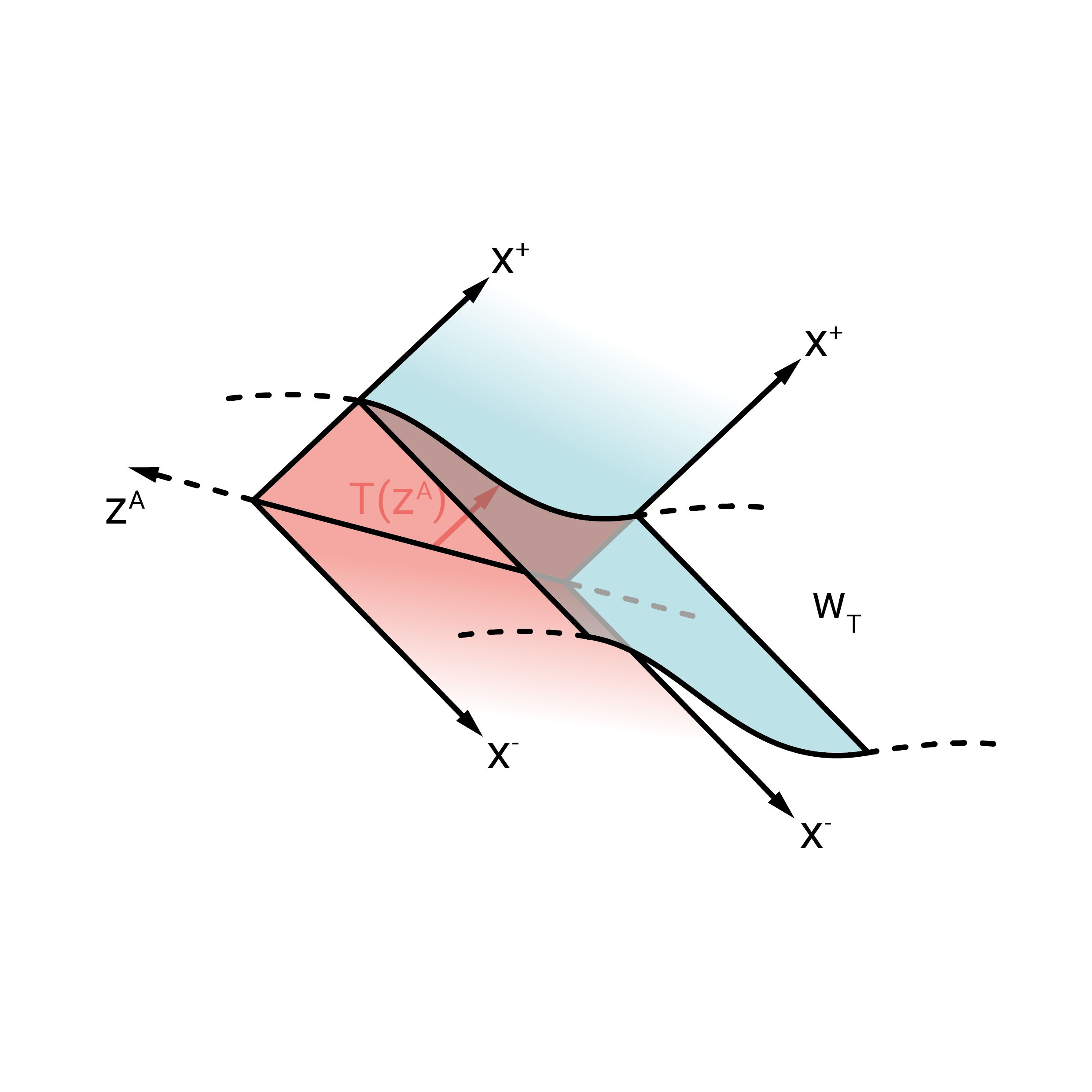
Figure 2: The shifted wedge $W_{T}$ is in blue, the original wedge in red. The edge of the shifted wedge is parameterized by a function $T(z^{A})$.

So we have two modular operators: One for $W$ and one for $W_{T}$. We know from Bisognano-Wichmann that $\Delta_{W}^{it}$ generates boosts, so points in $W_{T}$ get moved to points inside $W_{T}$ for positive values $t>0$ of the parameter. This situation is referred to as a “half sided modular inclusion” (modulo some other technical requirements [29]). If we have a half sided modular inclusion, then we get an interesting interplay between $\Delta_{W}$ and $\Delta_{W_{T}}^{it}$; in fact one can show:

• $\Delta_{W_{T}}^{it}\Delta^{-it}_{W}=e^{i(e^{2\pi t}-1){{\cal E}}_{T}}$,

• ${{\cal E}}_{T}\geq 0$ as an operator,

• The ${{\cal E}}_{T}$’s and boosts generate the Bondi-Metzner-Sachs group,

• ${{\cal E}}_{T}$ is the angle-averaged ANEC operator

  $${{\cal E}}_{T}=\int\left(\int_{-\infty}^{\infty}\Theta_{++}(x^{+},x^{-}=0,z^{A})dx^{+}\right)T(z^{A})\,dz,$$ (60)

• Since ${{\cal E}}_{T}\geq 0$ for all $T>0$, the ANEC holds!

  $${\rm ANEC}(z^{A})=\int_{-\infty}^{\infty}\Theta_{++}(x^{+},x^{-}=0,z)dx^{+}\geq 0$$ (61)

The first relation may look mysterious but it is just the relation for two boosts in a pair of coordinate systems related by a null translation. The BMS algebra reflects this and the fact that $T(z^{A})$, the amount of the null translation, may depend on the coordinates $z^{A}$ of the edge of the wedge.

The connection between ${{\cal E}}_{T}$ and the ANEC was in fact recognized only many years after the work by Borchers, Wiesbrock and others, see [5]. The ANEC is a very strong non-perturbative constraint on matrix elements of the stress energy operator. An alternative proof using traditional high-energy methods can also be given in CFTs [14]. The fact that matrix elements of the ANEC operator have signs give constraining relations in conformal bootstrap approach to CFTs; for such topics see e.g. [21].

A refinement of the ANEC is obtained from the so called “QNEC”, closely related also to the “quantum focussing conjecture” [2]:

$$2\pi\,\langle\psi|\Theta_{++}(x^{+},x^{-}=0,z^{A})|\psi\rangle\geq\frac{\delta^{2}}{\delta T(z^{A})^{2}}S_{T}(\psi)\bigg{|}_{T=x^{+}}$$ (62)

where $S_{T}(\psi)$ means the von Neumann entropy of the reduced density matrix $\operatorname{Tr}_{W_{T}^{\prime}}|\psi\rangle\langle\psi|$ for the shifted wedge $W_{T}$ of a pure state $|\psi\rangle$. Of course the right side of this equation does not have a sign and the von Neumann entropy $S$ isn’t actually well defined, but one can show that after integration over $x^{+}$ that the QNEC is formally implied by the following – well defined – statement [7]:

$$2\pi\inf_{u^{\prime}\in W^{\prime}\ {\rm unitary}}\langle u^{\prime}\psi|{\rm ANEC}(z^{A})|u^{\prime}\psi\rangle=-\frac{\delta}{\delta T(z^{A})}S_{T}(\psi|\Omega)\bigg{|}_{T=0}$$ (63)

where $S_{T}$ means the relative entropy for the reduced “density matrix” of the state $|\psi\rangle$ respectively the vacuum state $|\Omega\rangle$ associated with the shifted wedge $W_{T}$. The optimization is over all unitaries $u^{\prime}$ in the algebra associated with the opposite wedge $W^{\prime}$, i.e. the commutant (by Haag duality). Of course we may pick $u^{\prime}=1$ and then we get an inequality:

$$2\pi\langle\psi|{\rm ANEC}(z^{A})|\psi\rangle\geq-\frac{\delta}{\delta T(z^{A})}S_{T}(\psi|\Omega)\bigg{|}_{T=0}\quad(\geq 0\quad\text{by DPI})$$ (64)

The ANEC and QNEC as described have been proven rigorously [7] for a null line in Minkowski and the exact same proof carries over to a null generator of a bifurcate Killing horizon like Schwarzschild. For a general null geodesic in an arbitrary curved spacetime or a congruence representing an outgoing light-sheet as in the QNEC, neither the ANEC nor the QNEC hold but one expects that they are restored, modulo terms involving the expansion and shear, once backreaction effects are taken into account. It seems plausible to me that the ANEC and QNEC might be a fundamental property of semi-classical gravity.

8 Petz map, state recovery and improved DPI

The QNEC suggests that we should take a closer look at

$$S_{0}(\psi|\Omega)-S_{T}(\psi|\Omega)$$ (65)

for a finite shift $T(z^{A})$. If this quantity is small then we should learn something about the flux of the ANEC operator; basically this flux should be small and we should be able to recover the reduced density matrix of $|\psi\rangle$ to $W$ from the reduced density matrix of the shifted wedge $W_{T}$. This hints at a connection to the important topic of “state recovery”. State recovery asks the following question: Suppose we have a channel $T:{{\cal A}}_{B}\to{{\cal A}}_{A}$ with dual channel $\tilde{T}$ giving a state $\rho_{B}=\tilde{T}(\rho_{A})$ for system $B$ for each input state $\rho_{A}$ from $A$. In which sense can this be “approximately inverted”? In other words, we ask for a channel $R:{{\cal A}}\to{{\cal B}}$ such that $\rho_{A}$ and $\tilde{R}(\rho_{B})$ are “close” for a class of states? Typically, we think of $\tilde{T}$ as a noisy channel erasing some information, and we think of $\tilde{R}$ as the recovery channel. Not always can we recover the initial $\rho_{A}$ from $\rho_{B}=\tilde{T}(\rho_{A})$, but we should be able to do so approximately if only a small amount of information is erased relative to some reference state.

In the classical context we have a commutative algebra ${{\cal A}}_{A}$ of functions of a random variable $x$ (multiplication operators), and a density matrix corresponds to a probability distribution $p_{A}(x)$ via $\rho_{A}=\sum_{x}p_{A}(x)|x\rangle\langle x|$. Under these identifications, a (dual) channel $\tilde{T}$ from $A$ to $B$ acts on probability distributions by

$$p_{B}(y)=\sum_{x}\tilde{T}(y|x)p_{A}(x)$$ (66)

where the kernel $\tilde{T}(y|x)$ of the (dual) channel is a “stochastic map”, i.e. probability distribution in $y$. So the output state is $\rho_{B}=\sum_{y}p_{B}(y)|y\rangle\langle y|$.

A natural guess for defining the recovery channel, $\tilde{P}(x|y)$, which is inspired by Bayes’ rule is

$$\tilde{P}(x|y)=\frac{\tilde{T}(y|x)p_{A}(x)}{p_{B}(y)}$$ (67)

wherein $p_{A}$ is supposed to be a given reference probability distribution which in the quantum case will be a reference state for system $A$. We interpret $\tilde{T}(y|x)$ as the conditional probability of $y$ given $x$ and then the formula states Bayes’ theorem giving the conditional probability of $x$ given $y$.

Exercise 16. Suppose we have a channel $T:{{\cal A}}_{B}\to{{\cal A}}_{A}$ with dual channel $\tilde{T}$ and a reference state $\sigma_{A}$ on $A$. Then $\sigma_{B}=\tilde{T}(\sigma_{A})$ is a reference state on $B$. We assume that ${{\cal A}}_{A}$ and ${{\cal A}}_{B}$ are finite-dimensional matrix algebras such that the states are represented by density matrices. Check that the “Petz” recovery channel (for more on this see [22]):

$$\tilde{P}(\,.\,):=\sqrt{\sigma_{A}}T[\sqrt{\sigma_{B}}^{-1}(\,.\,)\sqrt{\sigma_{B}}^{-1}]\sqrt{\sigma_{A}}$$ (68)

acting on density matrices for $B$ reduces to Bayes’ formula (67) in the classical case (with $\sigma_{A}=\sum_{x}p_{A}(x)|x\rangle\langle x|$ etc.). Show that $\tilde{P}$ exactly recovers $\sigma_{A}$ from $\sigma_{B}$ and that, in general $\tilde{P}(\rho_{B})$ is a density matrix for system $A$ (which may or may not exactly recover $\rho_{A}$).

The Petz recovery channel described in exercise 16 is of course not the only non-commutative generalization of Bayes’ formula (67). What we want on general grounds is a recovery channel having the property that if, for some reference state $\sigma$ (the vacuum in our case), the information loss $S(\rho_{A}|\sigma_{A})-S(\tilde{T}(\rho_{A})|\tilde{T}(\sigma_{A}))$ is small, then the difference between $\rho_{A}$ and $\tilde{R}\tilde{T}(\rho_{A})$ is small in some sense. Given that the algebras of observables that we wish to deal with are of type III, we should also have definitions that work for general type.

The first task is relatively easy. Given $\sigma_{A}$ and $\sigma_{B}:=\tilde{T}(\sigma_{A})$ we first define the “KMS inner product” on ${{\cal A}}_{A}$:

$$\langle a_{1},a_{2}\rangle_{\sigma}=\langle\sqrt{\sigma_{A}}|a_{1}^{\dagger}\Delta_{A}^{1/2}a_{2}|\sqrt{\sigma_{A}}\rangle\quad(=\operatorname{Tr}(a_{1}^{\dagger}\sqrt{\sigma_{A}}a_{2}\sqrt{\sigma_{A}})\quad\text{when ${{\cal A}}_{A}=$ type I})$$ (69)

Here $\Delta_{A}=\Delta_{\sigma_{A},\sigma_{A}}$ is the modular operator for $\sigma_{A}$. We do the same for $B$ using $\sigma_{B}$. So we have KMS inner products on ${{\cal A}}_{A}$ and ${{\cal A}}_{B}$ and then via inner products, we can define an adjoint (depending on $\sigma_{A}$) $T^{+}:{{\cal A}}_{A}\to{{\cal A}}_{B}$ of the channel $T:{{\cal A}}_{B}\to{{\cal A}}_{A}$.

Exercise 17. Check that the Petz recovery channel $P$ in exercise 16 is precisely $T^{+}$.

We can also define the “rotated Petz map”

$$P_{t}=Ad(\Delta^{-it}_{B})\circ T^{+}\circ Ad(\Delta^{it}_{A})$$ (70)

where “Ad” means the Heisenberg time evolution $Ad(X)Y=XYX^{-1}$. Even more generally, we can define the “twirled Petz map” by averaging this against some probability density $w(t)$,

$$R=\int dtw(t)P_{t}$$ (71)

All three recovery maps, $P,P_{t},R$ reduce to Bayes’ inversion formula in the classical case. It turns out however that $R$ for the specific weight $w(t)=\frac{\pi}{\cosh(2\pi t)+1}$ understood from now on is a recovery channel with the desired property. Namely, one can show

$$S(\rho|\sigma)-S(\tilde{T}(\rho)|\tilde{T}(\sigma))\geq-\operatorname{ln}F(\rho|\tilde{R}\tilde{T}(\rho)),$$ (72)

where $F(\omega_{1}|\omega_{2})=(\operatorname{Tr}\sqrt{\sqrt{\omega_{1}}\,\omega_{2}\sqrt{\omega_{1}}})^{2}$ is the fidelity between two density matrices, which has a well-defined generalization to state functionals on arbitrary von Neumann algebra types where density matrices may not exist. For general von Neumann algebras, these statements were first shown in [11] (for inclusion channels), and for type I in [20]. If you don’t like the fidelity you can replace the right side also by $(1/4)\|\rho-\tilde{R}\tilde{T}(\rho)\|^{2}$ where the norm between the states is the “trace norm” (defined also for general von Neumann algebras), or by the measured relative entropy $S_{M}(\rho|\tilde{R}\tilde{T}(\rho))$. For proofs of these more general statements see [16].

Exercise 17. Show that if $\omega_{i}=|\chi_{i}\rangle\langle\chi_{i}|$ are pure states on the algebra of all bounded operators, then their fildelity is $|\langle\chi_{1}|\chi_{2}\rangle|^{2}$, i.e. the transition amplitude. Show that for any pair of density matrices $F\leq 1$ and $F=1$ if and only if $\omega_{1}=\omega_{2}$.

The inequality (72) is called an “improved” DPI. Its proof goes beyond these lecture notes but I mention that the operator $V$ used in the proof of the ordinary DPI also plays a major role, together with a host of other methods such as non-commutative $L_{p}$ norms, methods from complex analysis, and an interpolation theory for these norms.

Let us instead get a feeling for what the improved DPI says. Suppose first that $S(\rho|\sigma)-S(\tilde{T}\rho|\tilde{T}\sigma)=0$ exactly. Then $F(\rho|\tilde{R}\tilde{T}(\rho))=1$ and hence $\rho=\tilde{R}\tilde{T}(\rho)$ by exercise 17, so the state $\rho$ is recovered from $\tilde{T}(\rho)$ exactly.

9 DPI in the sky: Generalized second law

With the help of the ordinary DPI and the idea of half sided modular inclusion one can obtain the “generalized second law” of black hole thermodynamics in Schwarzschild spacetime in a semi-classical setting. The idea to use quantum information theoretic inequalities to get such a law first appeared in [25] to my knowledge. That the relative entropy should play a role in this context was observed by [4]. The reasoning that we shall present is essentially due to [28] though I will emphasize more strongly the importance of half-sided modular inclusions; see also [31] for a similar discussion.

Let us consider the exterior of the black hole and a thermal equilibrium state with respect to the time translations. I call the exterior the “right wedge” $W$ by analogy with Rindler space. It can be shown that this state can be extended to the analytic extension of the Schwarzschild spacetime, if and only if the temperature is $a/(2\pi)$, i.e. the Hawking temperature. This state $\omega$ is called the “Hartle-Hawking state”. By construction, its modular operator $\Delta$ for the algebra ${{\cal A}}_{W}$ corresponds to future directed boosts. More precisely,

$$\operatorname{ln}\Delta=\beta\int_{H^{+}}\Theta_{\mu\nu}K^{\mu}dS^{\nu}+\beta\int_{I^{+}}\Theta_{\mu\nu}K^{\mu}dS^{\nu}+\text{left wedge}$$ (73)

where “left wedge” is a corresponding contribution from the left (opposite) wedge not drawn in the figure which is over $H^{-}$ and $I^{-}$ in that wedge. $K^{\mu}$ is the generator of time translations which has the form $K=ax^{+}\partial_{+}$ on $H^{+}$ where $x^{+}$ is an affine parameter.

Consider next a Cauchy surface $\Sigma_{T}$ as in the following figure.

I can assume that with a suitable choice of affine parameter $x^{+}$ on the future horizon, this Cauchy surface will intersect the horizon at $x^{+}=T$. Applying boosts with positive boost parameter $t$ to $\Sigma_{T}$ gives another Cauchy surface, $\Sigma_{1}$ which is inside the domain of dependence $W_{T}$ of $\Sigma_{T}$. We are thus in the situation of a half-sided modular inclusion, and it follows that the modular operator $\Delta_{T}$ for the algebra ${{\cal A}}(W_{T})$ satisfies

$$\operatorname{ln}\Delta-\operatorname{ln}\Delta_{T}={\mathcal{E}}_{T}=aT\int dz\int_{-\infty}^{\infty}dx^{+}\Theta_{++}(x^{+},x^{-}=0,z)$$ (74)

Here $dz$ is the area element on horizon cross sections of constant $x^{+}$ (which could be written as $dz=r_{0}^{2}d^{d-2}\Omega$ more fully). Let us now consider another state $\rho$ on ${{\cal A}}_{W}$ with restriction $\rho_{T}$ to $W_{T}$. The DPI, i.e. monotonicity of the relative entropy tells us that

$$\partial_{T}S(\rho_{T}|\omega_{T})\leq 0.$$ (75)

By (74) and (73), we may formally write, with $\beta$ the inverse Hawking temperature,

$$\omega_{T}=Z_{T}^{-1}e^{-\beta H_{T}},\quad H_{T}=a\int_{T}^{\infty}dx^{+}\int dz\,(x^{+}-T)\Theta_{++}(x^{+},x^{-}=0,z)$$ (76)

Going from the relative entropy to the entropy I formally get

$$\partial_{T}S(\rho_{T})\geq a\beta\partial_{T}\int_{T}^{\infty}dx^{+}\int dz\,(x^{+}-T)\langle\Theta_{++}(x^{+},x^{-}=0,z)\rangle_{\rho}-\partial_{T}\operatorname{ln}Z_{T}.$$ (77)

It is plausible that the last term can be neglected because, formally, ${\mathcal{E}}_{T}$ acts as a translation and the corresponding $U(y):=e^{iy{{\cal E}}_{T}/a}$ is moving the algebras for the shifted wedges into each other in the sense that $U(y){{\cal A}}(W_{T})U(y)^{\dagger}={{\cal A}}_{W_{(1+y)T}}$, by the properties of half sided modular inclusions. Consequently, formally the free energies $\operatorname{ln}Z_{T}$ should be independent of $T$. If I neglect the last term and use $\beta=2\pi/a$, then I get

$$\partial_{T}S(\rho_{T})\geq-2\pi\int_{T}^{\infty}dx^{+}\int dz\,\langle\Theta_{++}(x^{+},x^{-}=0,z)\rangle_{\rho}.$$ (78)

In order to treat the term on the right side we can appeal to the Raychaudhuri equation and assume the semi-classical Einstein equation (58) to relate $R_{++}$ to $\langle\Theta_{++}\rangle_{\rho}$:

$$\partial_{+}\theta_{+}=-\frac{1}{d-2}\theta_{+}^{2}-\sigma_{+}^{2}-R_{++}=-\frac{1}{d-2}\theta_{+}^{2}-\sigma_{+}^{2}-8\pi G\langle\Theta_{++}\rangle_{\rho}$$ (79)

The shear-squared $\sigma_{+}^{2}$ and the expansion-squared $\theta_{+}^{2}$ are considered to be of higher order. Thus, under these assumptions/approximations we can write

$$-\int_{T}^{\infty}dx^{+}\int dz\,\langle\Theta_{++}(x^{+},x^{-}=0,z)\rangle_{\rho}.\approx\frac{1}{8\pi G}\int_{T}^{\infty}dx^{+}\int dz\,\partial_{+}\theta_{+}$$ (80)

Now suppose $A_{T}$ is the area of the horizon cross section at $x^{+}=T$. The expansion is the infinitesimal change in area cross section along a congruence of affine geodesics, so

$$\int_{T}^{\infty}dx^{+}\int dz\,\partial_{+}\theta_{+}=-\int_{x^{+}=T}dz\,\theta_{+}=-\partial_{T}A_{T}$$ (81)

Thus we see that

$$\partial_{T}\left(S(\rho_{T})+\frac{A_{T}}{4G}\right)\equiv\partial_{T}S_{\rm gen}\gtrsim 0$$ (82)

which is called the generalized second law. Note that the QFT piece should include all quantized perturbations around the spacetime background, including quantized gravitational perturbations. Note also that this derivation assumed a small change of the state $\rho_{0}$ since we ignored the expansion and shear squared terms. The $\gtrsim$ should thus become exact for an infinitesimal change. The derivation is independent of any of the objections raised in connection with the Bekenstein bound such as [27].

10 Applications of improved DPI: QNEC, generalized second law, holographic reconstruction

Let us apply the improved DPI to the situation where system $A$ is the wedge algebra ${{\cal A}}_{W}$ in Minkowski spacetime, system $B$ is the shifted wedge algebra ${{\cal A}}_{W_{T}}$, the channel $I:{{\cal A}}_{W_{T}}\subset{{\cal A}}_{W}$ is simply inclusion (so the dual channel $\tilde{I}$ on states is a “partial trace” over the causal complement of $W_{T}$ inside $W$) and the reference state $\sigma_{A}$ is the vacuum state $|\Omega\rangle$ or rather its reduction to $W$. The improved DPI, or rather, a stronger version of it with the “integral outside the fidelity”, can be shown to give [11], where we assume $T(z^{A})=T$ to be a positive constant:

$$\frac{1}{T}[S_{0}(\psi|\Omega)-S_{T}(\psi|\Omega)]\geq-\int_{T}^{\infty}\ln F_{0}(\psi|e^{ix_{+}P_{+}}\psi)\,\frac{dx_{+}}{x^{2}_{+}}.$$ (83)

Here I mean by $S_{T}$ the relative entropy for the reduced states (“density matrices”) of $|\psi\rangle,|\Omega\rangle$ to the shifted wedge $W_{T}$, and I mean by $S_{0}$ that to the original wedge $W$. Likewise $F_{0}$ is the fidelity between the reduced density matrices of $|\psi\rangle,e^{ix_{+}P_{+}}|\psi\rangle$ to $W$. $P_{+}$ is the momentum operator in the $x^{+}$ direction.

The above inequality can be seen as a cousin of the QNEC for finite $T>0$. To get a feeling for what it says, suppose that $\frac{1}{T}[S_{0}(\psi|\Omega)-S_{T}(\psi|\Omega)]\approx 0$, i.e. a nearly zero rate of change of $S_{T}$. For small $T$, the integral on the right side of the above inequality is dominated by the contribution from $x_{+}\approx T$. Therefore $\ln F_{0}(\psi|e^{iTP_{+}}\psi)\approx 0$ and hence $F_{0}(\psi|e^{iTP_{+}}\psi)\approx 1$, so the reduced density matrices of $|\psi\rangle$ and $e^{iTP_{+}}|\psi\rangle$ to $W$ are nearly the same. This will be the case if $|\psi\rangle$ is nearly an eigenstate for $e^{iTP_{+}}$ i.e. $|\psi\rangle=\int dp_{+}\psi(p_{+})|p_{+}\rangle$ for some wave function $\psi(p_{+})$ that is sharply peaked at integer multiples of $2\pi/T$. Intuitively, the position-space wave function $\hat{\psi}(x^{+})$ of such a nearly eigenstate is approximately periodic in $x^{+}$ with period $T$ as illustrated by the periodic cat images below. The inclusion channel basically discards the part of this wave function between $0\leq x^{+}\leq T$. However, for a nearly periodic wave function discarding any finite portion does not constitute a major loss of information, see the cat figure below, i.e. we can more or less restore the missing part by periodicity. In other words, it is intuitively clear that we can recover the original wave function with high precision if $\frac{1}{T}[S_{0}(\psi|\Omega)-S_{T}(\psi|\Omega)]\approx 0$, just as the improved DPI says.

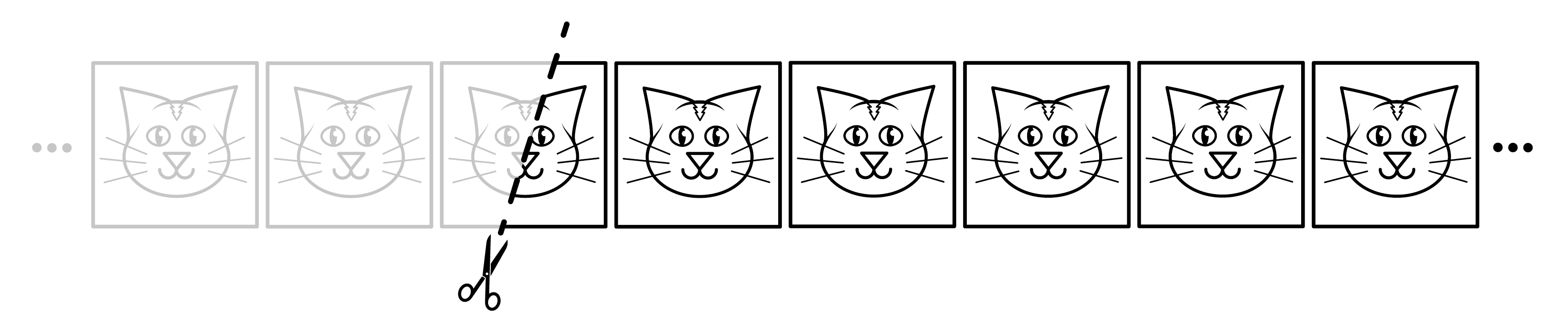
Figure 3: Discarding part of a (nearly) periodic state does not constitute an essential loss of information because the part that has been chopped off can be restored. Here $T$ from the main text is analogous to the width of an individual cat image.

Since the improved DPI gives a better bound for any inequality derived from the ordinary DPI, we get an improved version of the generalized second law. Setting $S_{\rm gen}=S_{\rm bh}+S_{\rm qft}$ and denoting as above the partial states on the Cauchy surfaces $\Sigma_{0}$ and $\Sigma_{1}$ by $\rho_{0}$ and $\rho_{1}$, we get for example

$$dS_{\rm gen}\gtrsim-\operatorname{ln}F_{\Sigma_{0}}(\rho_{0}|\tilde{R}\rho_{1}).$$ (84)

The recovery map $\tilde{R}$ is basically given by the same formula as in the case of Rindler horizons. As is intuitively clear, the increase in the generalized entropy controls the recoverability of the initial state on $\Sigma_{0}$ from the final state on $\Sigma_{1}$.

Holographic ideas, especially in the context of the AdS-CFT correspondence, suggest a relation between entropies in the gravitational bulk and the boundary CFT, at least in a semi-classical regime. Such ideas are intimately related to the Ryu-Takaynagi proposal [24] and its generalization [18] for holographic calculations of the entanglement entropy. In particular, in [19], it was shown that bulk- and boundary relative entropies $S(\rho_{a}|\sigma_{a})$ and $S(\rho_{A}|\sigma_{A})$ similar to those discussed above are approximately equal (up to order $1/N_{c}$) under an appropriate identification of the bulk and boundary regions $a$ and $A$. More precisely $a$ is a certain region whose boundary inside AdS-spacetime (the “HRRT surface” [24, 18]) is cohomlogous to a boundary region $A$. There is a channel $N:{{\cal A}}_{A}\to{{\cal A}}_{a}$ – the “AdS-CFT correspondence” – mapping boundary to bulk operators (the construction of which goes through a certain procedure involving a “code subspace” in the boundary Hilbert space from an information theoretic viewpoint on AdS-CFT) and $\sigma_{A}=\tilde{N}(\sigma_{a})$. The approximate equality between $S(\rho_{a}|\sigma_{a})$ and $S(\rho_{A}|\sigma_{A})$ yields a close connection to ideas of state recovery as described above, i.e. to a viewpoint where the AdS-CFT correspondence is seen as a kind of recovery problem: The inversion problem for the channel $N:{{\cal A}}_{A}\to{{\cal A}}_{a}$ is solved approximately by the twirled Petz map $R$, for many more details on such ideas see e.g. [8], which build on the ideas by [13]. For connections to the information loss paradox see e.g. [23].

Acknowledgements: I thank Tom Faulkner and Robert M. Wald for discussions about the generalized second law, Nima Lashakari for discussions about state recovery, and Thomas Endler from MPI-MiS for help with figures. I am grateful to the Max-Planck Society for supporting the collaboration between MPI-MiS and Leipzig U., grant Proj. Bez. M.FE.A.MATN0003.

References

- [1] Bisognano, Joseph J., and Eyvind H. Wichmann. “On the duality condition for a Hermitian scalar field”, Journal of Mathematical Physics 16.4 (1975): 985-1007.
- [2] Bousso, Raphael, et al. "Quantum focusing conjecture." Physical Review D 93.6 (2016): 064044, Bousso, Raphael, et al. "Proof of the quantum null energy condition." Physical Review D 93.2 (2016): 024017.
- [3] Buchholz, Detlev, Claudio D’Antoni, and Klaus Fredenhagen. "The universal structure of local algebras." Communications in Mathematical Physics 111.1 (1987): 123-135.
- [4] Casini, Horacio. “Relative entropy and the Bekenstein bound,” Class. Quant. Grav. 25, 205021 (2008) doi:10.1088/0264-9381/25/20/205021
- [5] Casini, Horacio, Eduardo Teste, and Gonzalo Torroba. "Modular Hamiltonians on the null plane and the Markov property of the vacuum state." Journal of Physics A: Mathematical and Theoretical 50.36 (2017): 364001, Faulkner, Thomas, et al. "Modular Hamiltonians for deformed half-spaces and the averaged null energy condition." Journal of High Energy Physics 2016.9 (2016): 1-35
- [6] Casini, Horacio, Javier M. Magán, and Pedro J. Martínez. "Entropic order parameters in weakly coupled gauge theories." Journal of High Energy Physics 2022.1 (2022): 1-58.
- [7] Ceyhan, Fikret, and Thomas Faulkner. "Recovering the QNEC from the ANEC." Communications in Mathematical Physics 377.2 (2020): 999-1045.
- [8] Cotler, Jordan, et al. "Entanglement wedge reconstruction via universal recovery channels." Physical Review X 9.3 (2019): 031011. Dong, Xi, Daniel Harlow, and Aron C. Wall. "Reconstruction of bulk operators within the entanglement wedge in gauge-gravity duality." Physical review letters 117.2 (2016): 021601. Harlow, Daniel. "The Ryu–Takayanagi formula from quantum error correction." Communications in Mathematical Physics 354.3 (2017): 865-912. Faulkner, Thomas, and Aitor Lewkowycz. "Bulk locality from modular flow." Journal of High Energy Physics 2017.7 (2017): 1-31.
- [9] Chandrasekaran, Venkatesa, et al. "An Algebra of Observables for de Sitter Space." arXiv preprint arXiv:2206.10780 (2022).
- [10] Driessler, W. "On the type of local algebras in quantum field theory." Communications in Mathematical Physics 53.3 (1977): 295-297.
- [11] Faulkner, Thomas, Stefan Hollands, Brian Swingle and Yixu Wang. "Approximate Recovery and Relative Entropy I: General von Neumann Subalgebras." Communications in Mathematical Physics 389.1 (2022): 349-397.
- [12] Fewster, Christopher J., and Thomas A. Roman. "Null energy conditions in quantum field theory." Physical Review D 67.4 (2003): 044003, Fewster, Christopher J., and Stefan Hollands. "Quantum energy inequalities in two-dimensional conformal field theory." Reviews in Mathematical Physics 17.05 (2005): 577-612, Ford, Larry H., and Thomas A. Roman. "Averaged energy conditions and quantum inequalities." Physical Review D 51.8 (1995): 4277, Flanagan, Eanna E., and Robert M. Wald. "Does back reaction enforce the averaged null energy condition in semiclassical gravity?." Physical Review D 54.10 (1996): 6233, Fewster, Christopher J., and Gregory J. Galloway. "Singularity theorems from weakened energy conditions." Classical and quantum gravity 28.12 (2011): 125009.
- [13] Hamilton, Alex, et al. "Holographic representation of local bulk operators." Physical Review D 74.6 (2006): 066009.
- [14] Hartman, Thomas, Sandipan Kundu, and Amirhossein Tajdini. "Averaged null energy condition from causality." Journal of High Energy Physics 2017.7 (2017): 1-30.
- [15] Hollands, Stefan, and Ko Sanders. Entanglement measures and their properties in quantum field theory. Vol. 34. Berlin/Heidelberg, Germany: Springer, 2018.
- [16] Faulkner, Thomas, and Stefan Hollands. "Approximate recoverability and relative entropy II: 2-positive channels of general von Neumann algebras." Letters in Mathematical Physics 112.2 (2022): 1-24. Hollands, Stefan. "Trace-and improved data processing inequalities for von Neumann algebras." arXiv preprint arXiv:2102.07479 (2021). Junge, Marius, and Nicholas LaRacuente. "Multivariate trace inequalities, p-fidelity, and universal recovery beyond tracial settings." arXiv preprint arXiv:2009.11866 (2020).
- [17] Ford, L. H., Adam D. Helfer, and Thomas A. Roman. "Spatially averaged quantum inequalities do not exist in four-dimensional spacetime." Physical Review D 66.12 (2002): 124012.
- [18] Hubeny, Veronika E., Mukund Rangamani, and Tadashi Takayanagi. "A covariant holographic entanglement entropy proposal." Journal of High Energy Physics 2007.07 (2007): 062.
- [19] Jafferis, Daniel L., et al. "Relative entropy equals bulk relative entropy." Journal of High Energy Physics 2016.6 (2016): 1-20.
- [20] Junge, Marius, et al. "Universal recovery maps and approximate sufficiency of quantum relative entropy." Annales Henri Poincaré. Vol. 19. No. 10. Springer International Publishing, 2018.
- [21] Koloğlu, Murat, et al. "The light-ray OPE and conformal colliders." Journal of High Energy Physics 2021.1 (2021): 1-110, Kravchuk, Petr, and David Simmons-Duffin. "Light-ray operators in conformal field theory." Journal of High Energy Physics 2018.11 (2018): 1-111.
- [22] Ohya, Masanori, and Dénes Petz. Quantum entropy and its use. Springer Science & Business Media, 2004.
- [23] Penington, Geoffrey. "Entanglement wedge reconstruction and the information paradox." Journal of High Energy Physics 2020.9 (2020): 1-84. Almheiri, Ahmed, et al. "The entropy of bulk quantum fields and the entanglement wedge of an evaporating black hole." Journal of High Energy Physics 2019.12 (2019): 1-47.
- [24] Ryu, Shinsei, and Tadashi Takayanagi. "Holographic derivation of entanglement entropy from the anti–de sitter space/conformal field theory correspondence." Physical review letters 96.18 (2006): 181602.
- [25] Sorkin, Rafael. “The statistical mechanics of black hole thermodynamics" gr-qc/9705006
- [26] Takesaki, Masamichi. Theory of operator algebras I-II. Berlin: Springer, 2003.
- [27] W. G. Unruh and R. M. Wald, Phys. Rev. D 25, 942 (1982); W. G. Unruh and R. M. Wald, Phys. Rev. D 27, 2271 (1983); M. A. Pelath and R. M. Wald, Phys. Rev. D 60, 104009 (1999) [arXiv:gr-qc/9901032]; R. M. Wald, Living Rev. Rel. 4, 6 (2001) [arXiv:gr-qc/9912119]. [4] D. Marolf and R. D. Sorkin, Phys. Rev. D 69, 024014 (2004) [arXiv:hep-th/0309218]; D. Marolf and R. Sorkin, Phys. Rev. D 66, 104004 (2002) [arXiv:hep-th/0201255].
- [28] Wall, Aron C. “The Generalized Second Law implies a Quantum Singularity Theorem,” Class. Quant. Grav. 30, 165003 (2013) [erratum: Class. Quant. Grav. 30, 199501 (2013)] doi:10.1088/0264-9381/30/19/199501, Wall, Aron C. “A proof of the generalized second law for rapidly changing fields and arbitrary horizon slices,” Phys. Rev. D 85, 104049 (2012) [erratum: Phys. Rev. D 87, no.6, 069904 (2013)] doi:10.1103/PhysRevD.85.104049, Wall, Aron C. "Ten proofs of the generalized second law." Journal of High Energy Physics 2009.06 (2009): 021.
- [29] Wiesbrock, Hans-Werner. “Half-sided modular inclusions of von-Neumann-algebras." Communications in Mathematical Physics 157.1 (1993): 83-92. Wiesbrock, Hans-Werner. “Conformal quantum field theory and half-sided modular inclusions of von-Neumann-Algebras." Communications in mathematical physics 158.3 (1993): 537-543. Araki, Huzihiro, and László Zsidó. “Extension of the structure theorem of Borchers and its application to half-sided modular inclusions." Reviews in Mathematical Physics 17.05 (2005): 491-543. Borchers, Hans-Jürgen. ‘On revolutionizing quantum field theory with Tomita’s modular theory." Journal of mathematical Physics 41.6 (2000): 3604-3673.
- [30] Witten, Edward. “APS Medal for Exceptional Achievement in Research: Invited article on entanglement properties of quantum field theory.” Reviews of Modern Physics 90.4 (2018): 045003.
- [31] Witten, Edward. “Black holes, singularity theorems and all that,” PiTP lecture notes, https://www.ias.edu/sites/default/files/video/grlecturesedited.pdf