Holes and magnetic polarons in a triangular lattice antiferromagnet

Abstract

The intricate interplay between charge motion and magnetic order in geometrically frustrated lattices is central for the properties of many two-dimensional quantum materials. The triangular lattice antiferromagnet is a canonical example of a frustrated system, and here we analyse the dynamics of a hole in such a lattice focusing on observables that have become accessible in a new generation of experiments. Using the $t$-$J$ model, we solve the problem exactly within linear spin wave theory in the limit of strong magnetic interactions, showing that the ground state is described by a coherent state of spin waves. The derivation highlights the crucial role played by the interaction between a static hole and the neighboring spins, which originates in the geometric frustration and has often been omitted in earlier works. Furthermore, we show that the non-equilibrium dynamics after a hole has abruptly been inserted at a lattice site is given exactly by a coherent state with time-dependent oscillatory coefficients. Physically, this describes a burst of magnetic frustration propagating through only two-thirds of the lattice sites, since a destructive interference of spin waves leaves spins parallel to that removed by the hole unperturbed. After the wave has propagated through the lattice, the magnetization relaxes to that of the ground state. We then use our analytical solution to benchmark the widely used self-consistent Born approximation (SCBA), showing that it is very accurate also for a triangular lattice. The magnetic polaron spectrum is analysed for general magnetic interactions using the SCBA, and we compare our results with those for a square lattice.

I Introduction

Understanding the competition between hole motion and magnetic order is a major challenge. The small doping limit of high-temperature superconductors is characterised by holes moving in a square lattice antiferromagnet (SAFM), such that a description of these processes constitute an important step towards understanding these complicated materials Anderson (1987); Lee et al. (2006); Emery (1987); Schrieffer et al. (1988); Dagotto (1994). Partly due to this connection, the vast majority of studies have focused on hole dynamics in a SAFM. The properties of a hole in other lattices is however also of fundamental interest. It was suggested that the inherent geometrical frustration of a two-dimensional triangular lattice leads to the formation of a resonating valence bond state with no long range order Anderson (1973). While such quantum liquid states may be realised for intermediate coupling strengths Szasz et al. (2020), it is now widely recognised from series expansions as well as numerical calculations that the ground state of a triangular lattice for strong coupling has long-range antiferromagnetic order based on the $120^{\circ}$ antiferromagnetic Néel state Capriotti et al. (1999); Zheng et al. (2006); White and Chernyshev (2007). The increased role of fluctuations due to frustration has been shown to lead to interesting effects on the spin wave spectrum of such a triangular lattice antiferromagnet (TAFM) Leung and Runge (1993); Chernyshev and Zhitomirsky (2009). It also gives rise to perculiar properties of hole dynamics and magnetic polarons in TAFMs Azzouz and Dombre (1996); Everts et al. (1998); Vojta (1999); Srivastava and Singh (2005); Trumper et al. (2004). Several crystals realise a triangular lattice, but a microscopic description of their properties remains an open question due to their complicated nature with many unknown parameters Shimizu et al. (2003); Maśka et al. (2004); Wang et al. (2004); Yamashita et al. (2008); Itou et al. (2008); Law and Lee (2017); Li et al. (2018); Ni et al. (2019); Bourgeois-Hope et al. (2019); Zhou et al. (2017).

Recent experiments using cold atoms in optical lattices have provided a wealth of new information regarding the motion of holes in fermionic spin systems Chiu et al. (2019); Brown et al. (2019); Koepsell et al. (2019); Ji et al. (2021); Koepsell et al. (2021). These experiments realise the Fermi-Hubbard model essentially perfectly and, moreover, their single site resolution gives access to the real space dynamics of fermions in the lattice. A new generation of experiments trapping bosonic Yamamoto et al. (2020) and fermionic Yang et al. (2021) atoms in triangular optical lattices promise to provide new and detailed experimental insights into magnetic frustration and hole dynamics. Moreover, recent breakthrough experiments using multilayers of atomically thin van der Waals materials have realised triangular moiré superlattices with tuneable Hubbard parameters, thereby opening up an exciting new platform for exploring geometrically frustrated lattices Cao et al. (2018); Tang et al. (2020); Balents et al. (2020); Wu et al. (2018).

Inspired by these developments, in this work we explore the properties of a hole in a TAFM as described by the $t$-$J$ model. We show that in the limit of strong magnetic interactions and within linear spin wave theory, the exact ground state is a coherent state describing a static hole dressed by spin waves. The dressing is due to an interaction between the hole and its neighbouring spins coming from the geometric frustration of the lattice, and it has no analogy for a bi-partite lattice. We then extend our exact results to the non-equilibrium dynamics following a hole injected into a lattice site, and show that the resulting propagation of spin waves through the lattice is described by a time-dependent coherent state. Interestingly, spins parallel to the spin removed by the hole are unaffected due to destructive interference, so that the wave of magnetic disorder only propagates through two-thirds of the lattice. Eventually, the magnetic disorder relaxes to that of the ground state. Our analytical solution enables us to benchmark the SCBA, which is known to be accurate on a square lattice, and we show that this holds for a triangular lattice as well. Finally, we analyse the properties of a hole and the formation of magnetic polarons for general interaction strengths and compare to the case of a square lattice.

The paper is structured as follows. We formulate the model in Sec. II and apply the slave-fermion representation together with linear spin-wave theory. In Sec. III, we derive analytical solutions for the ground state and the non-equilibrium dynamics following a hole suddenly created at a given lattice site. The SCBA is introduced in Sec. IV, where we compare it to the exact solution and use it to analyse magnetic polarons for general interaction strengths. Finally, we conclude and provide an outlook in Sec. V.

II Hole spin-wave Hamiltonian

We consider the $t$-$J$ model with the Hamiltonian $H=H_{t}+H_{J}$, where Chao et al. (1977); MacDonald et al. (1988); Eskes et al. (1994)

$$\hat{H}_{t}=-t\sum_{\langle\mathbf{i,j}\rangle}\sum_{\sigma}\left[\tilde{c}_{\mathbf{i,\sigma}}^{\dagger}\tilde{c}_{\mathbf{j,\sigma}}+\mathrm{h.c.}\right]$$ (1)

describes the electron hopping. The modified creation operator $\tilde{c}_{\mathbf{i}\sigma}^{\dagger}=\left(1-\hat{n}_{\mathbf{i},\bar{\sigma}}\right)c_{\mathbf{i},\sigma}^{\dagger}$ with $\hat{n}_{\mathbf{i},\sigma}=\hat{c}_{\mathbf{i},\sigma}^{\dagger}\hat{c}_{\mathbf{i},\sigma}$ the local number operator and $\bar{\sigma}$ the opposite spin of $\sigma$, is defined such that $H_{t}$ is restricted to the Hilbert space of singly occupied sites. Here, $\hat{c}_{\mathbf{i},\sigma}^{\dagger}$ create a fermion at lattice site $\mathbf{i}$ and spin $\sigma$. The $t$-$J$ model, therefore, naturally describes a system in which the repulsion between spin $1/2$ fermions is much larger than the available energy. The second term $\hat{H}_{J}$ quantifies an antiferromagnetic Heisenberg spin-exchange interaction,

$$\hat{H}_{J}=J\sum_{\langle\mathbf{i,j}\rangle}\left[\hat{S}_{\mathbf{i}}^{z}\hat{S}_{\mathbf{j}}^{z}+\frac{1}{2}\left(\hat{S}_{\mathbf{i}}^{+}\hat{S}_{\mathbf{j}}^{-}-\hat{S}_{\mathbf{j}}^{+}\hat{S}_{\mathbf{i}}^{-}\right)-\frac{\hat{n}_{\mathbf{i}}\hat{n}_{\mathbf{j}}}{4}\right].$$ (2)

Here $\hat{n}_{\mathbf{i}}=\hat{n}_{\mathbf{i},\uparrow}+\hat{n}_{\mathbf{i},\downarrow}$, and $J>0$ denotes the antiferromagnetic exchange energy. The spin operators are defined in the Schwinger representation as

$$\mathbf{\hat{S}}_{i}=\frac{1}{2}\sum_{\sigma\sigma^{\prime}}\hat{c}_{i,\sigma}^{\dagger}\mathbf{\sigma}_{\sigma\sigma^{\prime}}\hat{c}_{i,\sigma^{\prime}}$$ (3)

with $\mathbf{\sigma}=\left(\sigma^{x},\sigma^{y},\sigma^{z}\right)$ the vector of Pauli matrices.

While the triangular lattice with antiferromagnetic coupling was originally suggested to realise a resonating valence bond ground state Anderson (1973), it is now known from series expansions as well as numerical calculations that its ground state has long-range antiferromagnetic order based on the $120^{\circ}$ antiferromagnetic Néel state Capriotti et al. (1999); Zheng et al. (2006); White and Chernyshev (2007). This state may be generated in the $(x,y)$ plane from the ordering vector $\mathbf{Q}_{\mathrm{TAFM}}=\left(4\pi/3,0\right)$, such that a spin at position $\mathbf{r}_{i}$ has an angle $\theta_{\mathbf{i}}=\mathbf{r}_{i}\cdot\mathbf{Q}_{\mathrm{TAFM}}$ relative to the $z$-axis as illustrated in Fig. 1(a). The lattice may then be subdivided into three sublattices with ordered spin-directions differing by angles of $2\pi/3$. For the subsequent analysis, it is convenient to perform a local coordinate rotation by $\theta_{\mathbf{i}}$ so that all spins point along the same local coordinate axis. The associated SU(2) rotation matrix reads Chernyshev and Zhitomirsky (2009)

$$R_{\mathbf{i}}=\begin{bmatrix}\cos(\theta_{\mathbf{i}}/{2})&\sin(\theta_{\mathbf{i}}/{2})\\ -\sin(\theta_{\mathbf{i}}/{2})&\cos(\theta_{\mathbf{i}}/{2})\end{bmatrix}$$ (4)

and the rotated (primed) operators are

$$\hat{c}_{\mathbf{i},\sigma}^{\dagger\prime}=\sum_{\sigma^{\prime}}R_{\mathbf{i},\sigma\sigma^{\prime}}\hat{c}_{\mathbf{i},\sigma^{\prime}}^{\dagger},\qquad\mathbf{\hat{S}}_{i}^{\prime}=R_{\mathbf{i}}^{-1}\mathbf{\hat{S}}_{\mathbf{i}}R_{\mathbf{i}}.$$ (5)

Upon substitution into equations (1) and (2) one obtains a rotated $t$-$J$ model for which the Néel state is now an effective ferromagnet. This prescription is straightforwardly applied to the SAFM as well, with altered ordering vector $\mathbf{Q}_{\mathrm{SAFM}}=\left(\pi,\pi\right)$. We use units where the lattice constant and $\hbar$ both are unity.

II.1 Slave-fermion representation

To model the dynamics of the hole we adopt a slave-fermion representation Schmitt-Rink et al. (1988); Kane et al. (1989); Martinez and Horsch (1991); Liu and Manousakis (1991); Nielsen et al. (2021), which describes the system in terms of spinless fermionic holes created by the operators $\hat{h}_{\mathbf{i}}^{\dagger}$, and bosonic spin excitations created by the operators $\hat{s}_{\mathbf{i}}^{\dagger}$. We have $\tilde{c}_{\mathbf{i},\downarrow}^{\prime}=\hat{h}_{\mathbf{i}}^{\dagger}\hat{s}_{\mathbf{i}}$ and $\tilde{c}_{\mathbf{i},\uparrow}^{\prime}=\hat{h}_{\mathbf{i}}^{\dagger}\sqrt{1-\hat{h}_{\mathbf{i}}^{\dagger}\hat{h}_{\mathbf{i}}-\hat{s}_{\mathbf{i}}^{\dagger}\hat{s}_{\mathbf{i}}}$, where the square root factor ensures that $\tilde{c}_{\mathbf{i},\uparrow}$ is uneffective on any site that already contains a hole or spin-excitation. The spin-operators are written as $\hat{S}_{\mathbf{i}}^{+\prime}=\sqrt{1-\hat{h}_{\mathbf{i}}^{\dagger}\hat{h}_{\mathbf{i}}-\hat{s}_{\mathbf{i}}^{\dagger}\hat{s}_{\mathbf{i}}}\hat{s}_{\mathbf{i}}$ and $\hat{S}_{\mathbf{i}}^{z\prime}=(1-\hat{h}_{\mathbf{i}}^{\dagger}\hat{h}_{\mathbf{i}}-2\hat{s}_{\mathbf{i}}^{\dagger}\hat{s}_{\mathbf{i}})/2$. Substituting into the rotated $t$-$J$ model and truncating to second order we obtain

$$\begin{split}\hat{H}_{J}=\hat{H}_{\text{s}}+\frac{J}{4}\sum_{\langle\mathbf{i},\mathbf{j}\rangle}\sin\theta_{ij}\left[\bar{s}_{\mathbf{i}}\hat{h}_{\mathbf{j}}^{\dagger}\hat{h}_{\mathbf{j}}-\hat{h}_{\mathbf{i}}^{\dagger}\hat{h}_{\mathbf{i}}\bar{s}_{\mathbf{j}}\right]\end{split}$$ (6)

with $\theta_{ij}=\theta_{\mathbf{i}}-\theta_{\mathbf{j}}$. Here $\bar{s}_{\mathbf{i}}=\hat{s}_{\mathbf{i}}+\hat{s}_{\mathbf{i}}^{\dagger}$, and $\hat{H}_{\text{s}}$ is the quadratic spin-wave Hamiltonian that also appears in the usual Holstein-Primakoff transformation on the triangular lattice Chernyshev and Zhitomirsky (2009). Expressions for $\hat{H}_{s}$ and the hopping term $\hat{H}_{t}$ in the slave fermion representation are given in App. A.

The second term in Eq. (6) quantifies a $J$-dependent interaction between the holes and spin-waves, which is absent in the SAFM where $\theta_{ij}=\pm\pi$. Physically, we can understand this interaction as coming from the geometric frustration on the triangular lattice. The ordered state of any spin is stabilised by the simultaneous spin-exchange with its six nearest neighbours. As we illustrate in Fig. 1, if one spin is removed the neighbouring spins will adjust their direction away from the $120^{\circ}$ order to minimise the energy. This corresponds to introducing spin waves in the system. Indeed, inspecting Eq. (6) shows that this interaction describes a spin-excitation arising from a purely stationary hole in the lattice. We note that this term, which has no equivalence for a square lattice, has been omitted in earlier works describing hole dynamics in TAFMs using a slave-fermion representation Azzouz and Dombre (1996); Trumper et al. (2004) so that the creation of spin waves only comes from the hopping term $\hat{H}_{t}$, see App. A. Such an approximation must be expected to be accurate for $J\ll t$. As we shall demonstrate below, the $J$-dependent interaction between the hole and the spin waves is however important away from this regime and significantly alters the asymptotic large $J$ behavior of the hole.

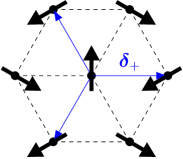
((a))

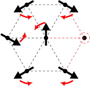
((b))

Figure 1: (a) The antiferromagnetic $120^{\circ}$ Néel state in a triangular lattice. The vectors ${\bf\it\delta}_{+}$ that define $g_{\mathbf{k}}$ and $\tilde{g}_{\mathbf{k}}$ are shown in blue. (b) Introducing a hole by removing a spin makes the neighbouring spins adjust their direction as indicated by the red arrows thereby introducing magnetic frustation. Here it is assumed that the spins exist in a much larger lattice which is not drawn.

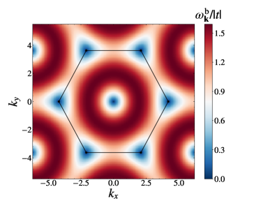
((a))

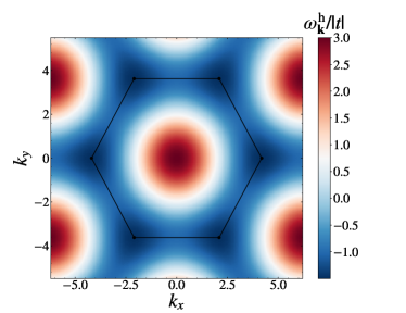
((b))

Figure 2: (a) Spin-wave dispersion $\omega_{\mathbf{k}}^{\mathrm{b}}$. (b) Hole dispersion $\omega_{\mathbf{k}}^{\mathrm{h}}$. Both for $J/\absolutevalue{t}=1$ and $t<0$.

Fourier transforming and diagonalizing the harmonic part of $H_{J}$ by the Bogoliubov transformation $\hat{s}_{\mathbf{k}}=u_{\mathbf{k}}\hat{b}_{\mathbf{k}}-v_{\mathbf{k}}\hat{b}_{-\mathbf{k}}^{\dagger}$, yields

$$\begin{split}\hat{H}&=\sum_{\mathbf{k}}\omega_{\mathbf{k}}^{\mathrm{h}}\hat{h}_{\mathbf{k}}^{\dagger}\hat{h}_{\mathbf{k}}+\sum_{\mathbf{k}}\omega_{\mathbf{k}}^{\mathrm{b}}\hat{b}_{\mathbf{k}}^{\dagger}\hat{b}_{\mathbf{k}}\\ &\qquad-\sum_{\mathbf{k},\mathbf{q}}\hat{h}_{\mathbf{k}+\mathbf{q}}^{\dagger}\hat{h}_{\mathbf{k}}\left[V_{\mathbf{k},\mathbf{q}}\hat{b}_{-\mathbf{q}}^{\dagger}-V_{\mathbf{k}+\mathbf{q},-\mathbf{q}}\hat{b}_{\mathbf{q}}\right].\end{split}$$ (7)

The hole and spin-wave dispersions are

$$\begin{split}\omega_{\mathbf{k}}^{\mathrm{h}}=-3tg_{\mathbf{k}},\qquad\omega_{\mathbf{k}}^{\mathrm{b}}=\frac{3}{2}J\sqrt{\left(1-g_{\mathbf{k}}\right)\left(1+2g_{\mathbf{k}}\right)},\end{split}$$ (8)

with the structure factor $g_{\mathbf{k}}=1/3\sum_{{\bf\it\delta}_{+}}\cos\left(\mathbf{k}\cdot{\bf\it\delta}_{+}\right)$ where $\mathbf{\delta}_{+}$ denotes a set of three nearest neighbour vectors illustrated in Fig. 1(a). These dispersions are shown in Fig. 2. Note that sign reversal symmetry with respect to $t$ is broken in a triangular lattice as opposed to a square lattice. The hole dispersion term, which is absent on a SAFM, arises from the fact that adjacent spins on the TAFM are not anti-parallel so that a hopping hole has a nonzero chance of projecting the displaced spin into the ”correct” state that agrees with the antiferromagnetic order. Hence even if just a single hole is present it may move across the lattice without frustrating the antiferromagnetic structure, which is impossible on the square lattice Trumper et al. (2004).

The vertex for the interaction between a hole and the spin waves is

$$V_{\mathbf{k,q}}= \frac{3\sqrt{3}i}{\sqrt{N}}t\left(v_{\mathbf{q}}\tilde{g}_{\mathbf{k}}+u_{\mathbf{q}}\tilde{g}_{\mathbf{k}+\mathbf{q}}\right)+\frac{3\sqrt{3}i}{4\sqrt{N}}J\left(u_{\mathbf{q}}-v_{\mathbf{q}}\right)\tilde{g}_{\mathbf{q}}$$

$$= V_{\mathbf{k,q}}^{t}+V_{\mathbf{q}}^{J}$$ (9)

with $\tilde{g}_{\mathbf{k}}=1/3\sum_{{\bf\it\delta}_{+}}\sin\left(\mathbf{k}\cdot{\bf\it\delta}_{+}\right)$ and

$$\begin{split}u_{\mathbf{k}}&=\frac{1}{2}\sqrt{\frac{2+g_{\mathbf{k}}}{\sqrt{\left(1-g_{\mathbf{k}}\right)\left(1+2g_{\mathbf{k}}\right)}}+2},\\ v_{\mathbf{k}}&=\frac{1}{2}\mathrm{sgn}(-g_{\mathbf{k}})\sqrt{\frac{2+g_{\mathbf{k}}}{\sqrt{\left(1-g_{\mathbf{k}}\right)\left(1+2g_{\mathbf{k}}\right)}}-2}.\end{split}$$ (10)

We see that it contains a term $V_{\mathbf{k,q}}^{t}\propto t$ arising from the hole hopping as well as a term $V_{\mathbf{q}}^{J}\propto J$. The latter is absent for a SAFM and arises from the geometric frustration shown in Fig. 1(b) as discussed above.

III Large $J/t$ limit

In this section, we present analytical solutions in the limit $J/t\gg 1$ both for the ground state and for a non-equilibrium situation where a hole is abruptly introduced in the lattice. The term $V_{\mathbf{q}}^{J}\propto J$ in Eq. (9) for the interaction vertex is clearly crucial for the properties of the hole in this limit, where it dresses the hole with spin waves. When this term is omitted as done in several previous works, the large magnetic interaction suppresses the motion of the hole and the ground state simply becomes a static hole surrounded by an unperturbed AF order, as for the SAFM. We show that when it is included, the problem can be mapped onto the well known Fröhlich model in the limit of infinite mass, which allows for an analytic solution describing an immobile hole surrounded by magnetic frustations.

In the $J/t\gg 1$ limit, we can neglect $\hat{H}_{t}$ and the Hamiltonian simplifies to

$$\hat{H}_{J}=\sum_{\mathbf{k}}\omega_{\mathbf{k}}^{\mathrm{b}}\hat{b}_{\mathbf{k}}^{\dagger}\hat{b}_{\mathbf{k}}-\sum_{\mathbf{k},\mathbf{q}}\hat{h}_{\mathbf{k}+\mathbf{q}}^{\dagger}\hat{h}_{\mathbf{k}}\left[V_{\mathbf{q}}^{J}\hat{b}_{\mathbf{q}}+V_{\mathbf{q}}^{J*}\hat{b}_{\mathbf{q}}^{\dagger}\right].$$ (11)

As is apparent from the real space representation of $\hat{H}_{J}$ given by Eq. (6), the hole is now stationary in the lattice where it emits or absorbs spin waves. Therefore, without loss of generality, we can assume the hole to be located at a certain lattice site $\mathbf{r}$. In the Hilbert space $\hat{h}_{\mathbf{r}}^{\dagger}\ket{\Psi_{\text{s}}}$ where $\ket{\Psi_{\text{s}}}$ is a general spin state of the lattice surrounding the hole, a straightforward calculation shows that the Hamiltonian in Eq. (11) is equivalent to

$$\hat{H}_{J}=\sum_{\mathbf{k}}\left[\omega_{\mathbf{k}}^{\mathrm{b}}\hat{b}_{\mathbf{k}}^{\dagger}\hat{b}_{\mathbf{k}}-V_{\mathbf{k}}^{J}\hat{b}_{\mathbf{k}}e^{i\mathbf{k}\cdot\mathbf{r}}+V_{\mathbf{k}}^{J*}\hat{b}_{\mathbf{k}}^{\dagger}e^{-i\mathbf{k}\cdot\mathbf{r}}\right].$$ (12)

After a gauge transform $\tilde{b}_{\mathbf{k}}=\hat{b}_{\mathbf{k}}e^{i\mathbf{k}\cdot\mathbf{r}}$, we obtain the Fröhlich Hamiltonian for an infinite mass impurity Mahan (2000).

III.1 Ground state

The Fröhlich Hamiltonian for infinite mass given by Eq. (12) can be solved analytically using the canonical transformation

$$\begin{split}\hat{\mathcal{S}}=e^{\sum_{\mathbf{k}}\left(\alpha_{\mathbf{k}}^{*}\tilde{b}_{\mathbf{k}}^{\dagger}-\alpha_{\mathbf{k}}\tilde{b}_{\mathbf{k}}\right)},\end{split}$$ (13)

where $\alpha_{\mathbf{k}}=V_{\mathbf{k}}^{J}/\omega_{\mathbf{k}}^{\mathrm{b}}$. Indeed,

$$\hat{\mathcal{S}}^{-1}\hat{H}_{J}\hat{\mathcal{S}}=\sum_{\mathbf{k}}\omega_{\mathbf{k}}^{\mathrm{b}}\tilde{b}_{\mathbf{k}}^{\dagger}\tilde{b}_{\mathbf{k}}+E_{g}$$ (14)

with

$$E_{g}=-\sum_{\mathbf{k}}\frac{\absolutevalue{V_{\mathbf{k}}^{J}}^{2}}{\omega_{\mathbf{k}}^{\mathrm{b}}}=-0.144\ J$$ (15)

the ground state energy, where the numerical value is obtained for an infinite lattice. The wave function of the ground state $\ket{\Psi_{\mathbf{r},g}}$ is a multimode coherent state of spin-waves,

$$\begin{split}\ket{\Psi_{\mathbf{r},g}}=\hat{\mathcal{S}}\ket{h_{\mathbf{r}}}=e^{-\frac{1}{2}\sum_{\mathbf{k}}\absolutevalue*{\alpha_{\mathbf{k}}}^{2}}e^{\sum_{\mathbf{k}}\alpha_{\mathbf{k}}^{*}\tilde{b}_{\mathbf{k}}^{\dagger}}\ket{h_{\mathbf{r}}},\end{split}$$ (16)

with $\ket{h_{\mathbf{r}}}=\hat{h}_{\mathbf{r}}^{\dagger}\ket{{\text{AF}}}$ where $\ket{\text{AF}}$ is the antiferromagnetic ground state defined by $\hat{b}_{\mathbf{k}}\ket{\mathrm{AF}}=0$. It follows from Eq. (16) that the ground state is an eigenfunction of $b_{\mathbf{k}}$ with eigenvalue $\alpha_{\mathbf{k}}^{*}$ and that the spin-wave distribution in any given mode is Poissonian

$$\begin{split}\bar{n}_{\mathbf{k},g}=\absolutevalue*{\alpha_{\mathbf{k}}}^{2},\qquad\sigma_{\mathbf{k},g}=\sqrt{\bar{n}_{\mathbf{k},g}}.\end{split}$$ (17)

Here $\bar{n}_{\mathbf{k},g}$ denotes the mean spin-wave number in mode $\mathbf{k}$ and $\sigma_{\mathbf{k},g}$ the standard deviation. From Eq. (16), it is also straightforward to compute the quasiparticle residue

$$Z=\absolutevalue*{\innerproduct*{h_{\mathbf{r}}}{\Psi_{\mathbf{r},g}}}^{2}=e^{-\sum_{\mathbf{k}}\absolutevalue*{\alpha_{\mathbf{k}}}^{2}}=0.8003,$$ (18)

which quantifes the overlap of the ground state with the state of a localised hole surrounded by unperturbed AF order. Since $Z>0$, the ground state corresponds to a well-defined quasiparticle, i.e. a magnetic polaron with infinite mass. The value $Z=0.8003$ should be contrasted to the case of a SAFM, where $Z\rightarrow 1$ for $J/|t|\rightarrow\infty$. This is because a stationary hole introduces magnetic frustration in a TAFM as shown in Fig. 1, in contrast to the case of a SAFM,.

III.2 Time-dependent many-body wave function

We now show that in addition to the ground state, we can also derive an analytical solution for the non-equilibrium many-body dynamics after a hole is abruptly introduced at a given lattice site. Such a quench experiment was recently performed for a SAFM Ji et al. (2021).

We imagine a hole created at lattice site ${\mathbf{r}}$ at time $\tau=0$ so that the initial state is $\ket{h_{\mathbf{r}}}=\hat{h}_{\mathbf{r}}^{\dagger}\ket{{\text{AF}}}$. The subsequent evolution of this state is given by

$$\ket*{\Psi_{\mathbf{r}}(\tau)} =e^{-i\hat{H}_{J}\tau}\ket*{h_{\mathbf{r}}}$$

$$=e^{-iE_{J}\tau}\hat{\mathcal{S}}e^{-i\sum_{\mathbf{k}}\omega_{\mathbf{k}}^{\mathrm{b}}\tilde{b}_{\mathbf{k}}^{\dagger}\tilde{b}_{\mathbf{k}}\tau}\hat{\mathcal{S}}^{-1}\ket*{h_{\mathbf{r}}}.$$ (19)

Equation (19) can be solved giving

$$\begin{split}\ket*{\Psi_{\mathbf{r}}(\tau)}&=e^{-iE_{J}\tau}e^{-\sum_{\mathbf{k}}\absolutevalue*{\alpha_{\mathbf{k}}}^{2}\left(1-e^{-i\omega_{\mathbf{k}}^{\mathrm{b}}\tau}\right)}\\ &\qquad\times e^{\sum_{\mathbf{k}}\alpha_{\mathbf{k}}^{*}\left(1-e^{-i\omega_{\mathbf{k}}^{\mathrm{b}}\tau}\right)\tilde{b}_{\mathbf{k}}^{\dagger}}\ket*{h_{\mathbf{r}}}.\end{split}$$ (20)

An equivalent wave function was recently obtained in a different context concerning an impurity in a Bose-Einstein condensate Shashi et al. (2014). Equation (20) shows that the many-body system is in a coherent state with time-dependent coefficients. The spin-wave number statistics is correspondingly time dependent with

$$\begin{split}\bar{n}_{\mathbf{k}}(\tau)=2\absolutevalue*{\alpha_{\mathbf{k}}}^{2}[1-\cos(\omega_{\mathbf{k}}^{\mathrm{b}}\tau)],\ \sigma_{\mathbf{k}}(\tau)=\sqrt{\bar{n}_{\mathbf{k}}(\tau)}.\end{split}$$ (21)

Since the oscillatory terms in Eq. (21) cancel upon integrating over the Brillouin zone (BZ) in the large time limit $\tau\gg 1/J$, the total number of spin-waves $\sum_{\mathbf{k}}\bar{n}_{\mathbf{k}}(\tau)$ in the non-equilibrium state approaches twice the total number in the ground state $\sum_{\mathbf{k}}\bar{n}_{\mathbf{k},g}$.

III.3 Local magnetization

We now analyse the local magnetization around the hole as a function of the time $\tau$ after it was created. The magnetization of the TAFM in the absence of the hole is

$$M_{\mathrm{AF}} =\frac{1}{N}\sum_{\mathbf{r}}\matrixelement*{\mathrm{AF}}{\hat{S}_{\mathbf{r}}^{z^{\prime}}}{\mathrm{AF}}=\frac{1}{2}-\frac{1}{N}\sum_{\mathbf{r}}\matrixelement*{\mathrm{AF}}{\hat{s}_{\mathbf{r}}^{\dagger}\hat{s}_{\mathbf{r}}}{\mathrm{AF}}$$

$$=\frac{1}{2}-\frac{1}{N}\sum_{\mathbf{k}}v_{\mathbf{k}}^{2}=0.2387.$$ (22)

As explained in Sec. II, the spin operators are rotated locally and a classical $120^{\circ}$ AFM state shown in Fig. 1(a) would give $M_{\mathrm{AF}}=\frac{1}{2}$. Equation (22) shows that quantum fluctuations reduce this ordering significantly.

When the hole is created at site $\mathbf{r}$ and time $\tau=0$, it distorts the magnetization in its surroundings. To quantify this, we calculate the local magnetization at site $\mathbf{r}+\mathbf{d}$

$$\begin{split}M(\tau,\mathbf{d})=\frac{\expectationvalue*{\hat{S}_{\mathbf{r}+\mathbf{d}}^{z^{\prime}}}_{\mathbf{r}}(\tau)}{M_{\mathrm{AF}}},\end{split}$$ (23)

where $\expectationvalue{\ldots}_{\mathbf{r}}(\tau)=\matrixelement*{\Psi_{\mathbf{r}}(\tau)}{\ldots}{\Psi_{\mathbf{r}}(\tau)}$ gives the time dependent expectation value. With this definition, $M(\tau,\mathbf{d})=1$ if a spin is unaffected by the presence of the hole. After Fourier transforming Eq. (23) to crystal momentum space, we use that since $\ket*{\Psi_{\mathbf{r}}(\tau)}$ is a coherent state, any spin-wave correlator factors into a product of single operator expectation values. As detailed in App. B, this gives

$$\begin{split}M(\tau,\mathbf{d})=\frac{M_{\mathrm{AF}}-\absolutevalue{\mathcal{A}_{\tau,\mathbf{d}}\left[u\right]-\mathcal{A}_{\tau,\mathbf{d}}^{*}\left[v\right]}^{2}}{M_{\mathrm{AF}}}\end{split}$$ (24)

where

$$\begin{split}\mathcal{A}_{\tau,\mathbf{d}}\left[u\right]&=\frac{1}{N}\sum_{\mathbf{q}}e^{i\mathbf{q}\cdot\mathbf{d}}\sqrt{N}\expectationvalue*{\tilde{b}_{\mathbf{q}}}_{\mathbf{r}}(\tau)\ u_{\mathbf{q}},\\ \mathcal{A}_{\tau,\mathbf{d}}\left[v\right]&=\frac{1}{N}\sum_{\mathbf{q}}e^{i\mathbf{q}\cdot\mathbf{d}}\sqrt{N}\expectationvalue*{\tilde{b}_{\mathbf{q}}}_{\mathbf{r}}(\tau)\ v_{\mathbf{q}}.\end{split}$$ (25)

and

$$\begin{split}\expectationvalue*{\tilde{b}_{\mathbf{q}}}_{\mathbf{r}}(\tau)=\alpha_{\mathbf{k}}^{*}\left(1-e^{-i\omega_{\mathbf{k}}^{\mathrm{b}}\tau}\right).\end{split}$$ (26)

Equations (24)-(26) describe how the magnetic frustration propagates through the lattice after the hole has been created. For long times $\tau\gg 1/J$, the oscillatory terms in Eq. (25) cancel upon integration over the BZ so that $M(\tau,\mathbf{d})$ tends to an asymptotic value. Since the magnetization only depends on the state through $\expectationvalue{b_{\mathbf{q}}}_{\mathbf{r}}(\tau)$, this asymptotic magnetization in fact coincides exactly with that of the ground state polaron, where $\expectationvalue{b_{\mathbf{k}}}_{\mathbf{r},g}=\alpha_{\mathbf{k}}^{*}$. This is somewhat surprising since there are twice as many spin waves in the lattice for long times as compared to the ground state polaron. Even more explicitly, the overlap between the time-dependent state and the polaron ground state is $|\bra*{\Psi_{\mathbf{r},g}}\ket*{\Psi_{\mathbf{r}}(\tau)}|^{2}=Z=0.8003<1$ since the time evolution just gives a phase factor, which shows the difference between the two states. The fact that the magnetization for long time matches that of the ground state is a direct consequence of the factorization of spin-wave correlators in a coherent state, which leads to cancellation of all time-dependent phase factors. More generally, the expectation value of any local observable, including higher order correlators, will approach that obtained from the ground state in the limit $\tau\gg 1/J$.

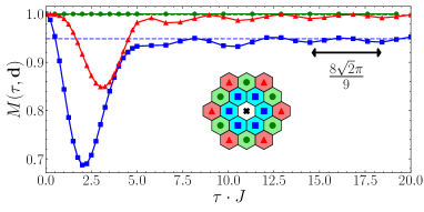
Figure 3: Magnetization $M(\tau,\mathbf{d})$ as a function of time $\tau$ for lattice sites near the hole, indicated by a black cross. Equivalent lattice sites have the same colour. Horizontal lines show the asymptotic limit obtained from the ground state polaron wave function given by Eq. (16). The black horizontal arrow shows a single oscillation period obtained from the stationary phase expansion.

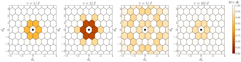
Figure 4: Magnetization surrounding a hole (black cross) for four different times after it was created. Each tile represents a spin and its color gives the magnetization. White tiles have an unperturbed magnetization $M(\tau,\mathbf{d})=1$.

In Fig. 3, the magnetization around a stationary hole is plotted as a function of time $\tau$ after it was created. This is obtained by numerically evaluating Eqs. (24)-(26). After the creation of the hole, we see a $30\ \%$ suppression of the magnetization at its nearest neighbours at time $\tau\sim 2/J$. After this initial ”burst” of magnetic frustration, the magnetization of the nearest neighbours relax towards a time-independent value coinciding with that of the ground state polaron as discussed above. With some lag, the frustration is then carried through to the sites further away, which show a similar initial decrease in magnetization although with a smaller amplitude and a subsequent relaxation to the ground state value.

Since the propagation of the magnetic frustration is carried by spin waves, one can calculate the period $T_{M}$ of the oscillations seen in Fig. 3 using the stationary phase method, which gives $T_{M}=2\pi/\omega_{\mathbf{k}_{0}}$. Here $\mathbf{k}_{0}$ denotes the dominant stationary points where $\gradient\omega_{\mathbf{k}}^{\mathrm{b}}=0$, which form an approximate circle around the origin, see Fig. 2(a). From this, we obtain

$$T_{M}=\frac{8\sqrt{2}\pi}{9J}.$$ (27)

Figure 4 shows that this result is indeed confirmed by the numerics.

Intriguingly, Fig. 3 shows that the magnetization at the green lattice sites is unperturbed by the presence of the hole for all times. As detailed in App. C, this fact follows from the symmetry properties of the triangular lattice. Using those, one can show that spins located at horizontal distances

$$\begin{split}d_{x}=\frac{3}{2}n\ \forall\ n\in\mathbb{Z}\end{split}$$ (28)

do not feel any disturbing influence from the presence of the hole. For these spins, which all point in the same direction as the spin that was originally at the location of the hole, the spin waves destructively interfere so that the magnetization remains unperturbed.

To further illustrate how the magnetic frustration propagates through the lattice after the hole has been created, we plot in Fig. 4 the magnetization in a larger region around the hole for four different values of propagation time $\tau$. Here, one clearly observes how a wave of disorder ripples through the lattice. Again, the sites that obey Eq. (28) are completely unaffected, such that the wave only travels through two of the three sublattices. In the last panel of Fig. 4, the asymptotic steady state is attained, where the spin ordering has relaxed to the polaron ground state value.

IV SCBA analysis

Having analysed in detail the large $J$ regime where hole is stationary, we now examine general values of $J/t$. In this case, the hopping of the hole driven by $\hat{H}_{t}$ will lead to additional dressing by magnetic frustration and the problem cannot be solved exactly.

We analyse the problem via the retarded Green’s function of the hole, which in frequency and momentum space reads

$$\begin{split}G(\mathbf{k},\omega)=\frac{1}{\omega-\omega_{\mathbf{k}}^{\mathrm{h}}-\Sigma(\mathbf{k},\omega)},\end{split}$$ (29)

where we have suppressed an infinitesimal positive imaginary part to the frequency $\omega+i\eta^{+}$. The self-energy $\Sigma(\mathbf{k},\omega)$ is calculated using the self-consistent Born approximation (SCBA), which is known to be very accurate for the equilibrium properties of a hole in a SAFMSchmitt-Rink et al. (1988); Kane et al. (1989); Martinez and Horsch (1991); Liu and Manousakis (1991). Recently, the accuracy of the SCBA was established for the non-equilibrium case as well where it was shown to agree very well with experimental data on a SAFM Nielsen et al. (2022).

In the SCBA, the self-energy is evaluated using all non-crossing diagrams leading to the self-consistent equation

$$\Sigma(\mathbf{k},\omega)=\sum_{\mathbf{q}}\frac{\absolutevalue{V_{\mathbf{k},\mathbf{q}}}^{2}}{\omega-\omega_{\mathbf{q}}^{\mathrm{b}}-\omega_{\mathbf{k}+\mathbf{q}}^{\mathrm{h}}-\Sigma(\mathbf{k+q},\omega-\omega_{\mathbf{q}}^{\mathrm{b}})}.$$ (30)

We solve this on a finite momentum grid by iteration starting from $\Sigma(\mathbf{k},\omega)=0$. The grid is created assuming a regular hexagonal lattice of side length $l$, with periodic boundary conditions such that the total number of independent lattice sites equals $N=3l^{2}$ Azzouz and Dombre (1996). As an example, we show in Fig. 5 the grid for the case $l=4$.

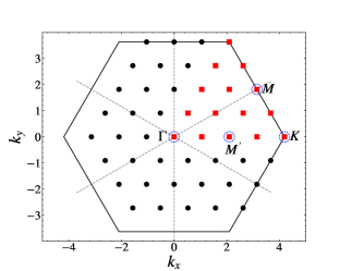
Figure 5: Momentum grid in the BZ for $l=4$ with the independent states highlighted as red squares. The momentum states $\Gamma\equiv(0,0)$, $M^{\prime}\equiv(2\pi/3,0)$, $K\equiv(4\pi/3,0)$ and $M\equiv(\pi,\sqrt{\pi/3})$ are shown. The symmetry axes of the structure factors used in deriving Eq. (28) are shown as grey dashed lines.

Due to the $C_{3}$ rotation and $y$-inversion symmetry of the BZ, we only need to evaluate the slice shown in red in Fig. 5. In the numerics, we use a lattice dimension $l=20$, giving a total of $1200$ spins. For convergence, we use a broadening $\eta_{+}/\absolutevalue{t}=0.01$.

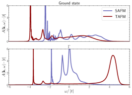
((a))

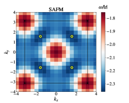
((b))

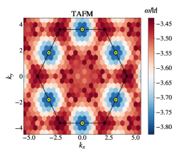
((c))

Figure 6: (a) Top panel: The hole spectral functions $A(\mathbf{k},\omega)$ within SCBA for $J/\absolutevalue{t}=0.3$ and $t<0$ for the ground state, corresponding to the momentum $M$ in the BZ for the TAFM and the momentum $(\pi/2,\pi/2)$ for the SAFM. Bottom panel: The spectral functions for zero momentum. (b) and (c) show the polaron dispersion in the full BZ for the SAFM.

IV.1 Magnetic polarons

We now explore the properties of the hole focusing on $t<0$, since the polaron is strongly suppressed except for special points in the BZ for $t>0$ Trumper et al. (2004).

In the top panel of Fig. 6(a), we plot the hole spectral function $A(\mathbf{k},\omega)=-2\text{Im}G(\mathbf{k},\omega)$ for $J/\absolutevalue{t}=0.3$ and the momentum labelled by the point $M$ in the BZ shown in Fig. 5. We see a clear quasiparticle peak at the energy $\omega/|t|\simeq-3.84$, which we interpret as the energy of the magnetic polaron. It turns out that this is the ground state as the polaron energies for other momenta are higher. For comparison, we also show the spectral function for the hole in a SAFM for the momentum $\mathbf{k}=(\pi/2,\pi/2)$ exhibiting a polaron peak at the energy $\omega/|t|\simeq-2.4$, which also corresponds to the ground state. Interestingly the ground state spectral functions for the two lattices are quite similar with a clear polaron peak at low energy, followed by a continuum with several smaller resonances. These peaks have been identified as string excitations in the case of a SAFM, corresponding to the hole oscillating in a linear potential formed by misaligned spins in its wake Manousakis (2007), and in analogy we can make the same identification for the case of the TAFM Trumper et al. (2004).

In the bottom panel of Fig. 6(a), the spectral function is plotted for zero momentum. Again, we see clear polaron peaks for both the TAFM and the SAFM. In addition, the spectral function for the TAFM has a broad new resonance appearing at $\omega\approx 4.5\absolutevalue{t}$ that may be interpreted as originating from the bare hole kinetic energy, see Fig. 2(b) Trumper et al. (2004). If the spectral function is tracked varying the momentum from the origin $\Gamma$ of the BZ towards the point $M$ on the edge, we observe that this high energy resonance smoothly evolves into the ground state polaron consistent with the hole dispersion.

Finally, we show in Figs. 6(b) and 6(c) the polaron dispersions in the full BZ obtained by solving $\omega_{\mathbf{k}}-\omega_{\mathbf{k}}^{\mathrm{h}}-\mathrm{Re}\Sigma(\mathbf{k},\omega_{\mathbf{k}})=0$. This illustrates the differences between the energy bands of the polaron in the SAFM and the TAFM.

IV.2 Polaron properties as a function of $J/|t|$

As we discussed above, there is no clear separation between a weak and a strong coupling regime for a hole in a TAFM, since the interaction vertex given by Eq. (9) has a term $\propto J$ in addition to a term $\propto t$. This is in contrast to the SAFM, where there is no interaction term $\propto J$ so that $J/|t|\gg 1$ corresponds to weak coupling. Therefore, we study in this section the properties of the polaron as a function of $J/|t|$. This will also allow us to make an important benchmarking of the SCBA by comparing it with the exact solution for $J\gg t$ derived in Sec. III.

The top panel in Fig. 7 plots the polaron energy as a function of $J/|t|$ ($t<0$) for the ground state momentum and the momentum at the point $K$ in the BZ, see Fig. 5. We see that the energies depend non-monotonically on $J/|t|$ exhibiting a maximum for intermediate values. In the limit of large $J/|t|$, the SCBA predicts the polaron energies approach the asymptotic values $\omega_{\mathbf{k}}\simeq-0.129J$ and $\omega_{\mathbf{k}}\simeq-0.133J$ for the $K$ and $M$ points respectively. Importantly, this deviates by less than $10\%$ from the exact result given by Eq. (15) for $J/|t|\rightarrow\infty$, which indicates that the SCBA is accurate also for the TAFM in addition to its well-known precision for the SAFM.

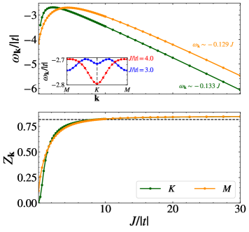
Figure 7: The polaron energy $\omega_{\mathbf{k}}$ (top panel) and quasi-particle residue $Z_{\mathbf{k}}$ (lower panel) as a function of $J/\absolutevalue{t}$ for $t<0$. The asymptotic slope of the dispersion for large $J$ is shown for each mode, and the exact large-$J$ quasi-particle residue from the coherent state solution is shown as a dotted line. The inset shows the polaron energy along the edge of the BZ, starting from $M$, passing through $K$, and returning to $M$ for two values of $J/\absolutevalue{t}$ on either side of the crossing point of the $M$ and $K$ modes, showing the discontinous jump in the ground state momentum.

In the regime $J/|t|\gg 1$, the momentum dependence of the polaron energy can be calculated perturbatively to first order in $t$ from the hole kinetic energy term in Eq. (7). Since the hole dispersion $\omega_{\mathbf{k}}^{\text{h}}$ has a minimum at the K point for $t<0$, see Figs. 2(b), the magnetic polaron also has a minimum at this momentum for large $J/|t|$ as can be seen from Fig. 6(c). As a result, the ground state momentum changes discontinuously with increasing $J/|t|$ as is illustrated further in the inset of Fig. 7.

The bottom panel in Fig. 7 plots the quasiparticle residues of the polarons calculated as $Z_{\mathbf{k}}=[1-\partial_{\omega}\mathrm{Re}\Sigma(\mathbf{k},\omega)\large|_{\omega=\omega_{\mathbf{k}}}]^{-1}$ Mahan (2000). When $J/|t|\rightarrow 0$, the residues go to zero reflecting that a large hopping leads to a strongly dressed hole and an eventual disappearance of the magnetic polaron like in the case of the magnetic polaron in a SAFM. The residues increase with $J/\absolutevalue{t}$ and converge to an asymptotic value for $J/\absolutevalue{t}\gg 1$, which overestimates the exact result $Z=0.8003$ given by Eq. (18) by just $3\%$. In App. F, we show that this remarkable accuracy of the SCBA in a TAFM can can be attributed to the coherent state coefficients $\alpha_{\mathbf{k}}=V_{\mathbf{k}}^{J}/\omega_{\mathbf{k}}^{\mathrm{b}}$, whose absolute value is generally much smaller than unity.

V Conclusion and outlook

We explored the equilibrium and non-equilibrium dynamics of a hole in a triangular lattice of anti-ferromagnetic spins, using the $t$-$J$ model in a slave fermion representation and linear spin wave theory. In the limit of strong magnetic coupling, we derived an exact solution showing that the ground state is a polaron consisting of a static hole dressed by a coherent state of spin waves, which is a direct consequence of the geometric frustration of the lattice. We also provided an exact solution for the dynamics ensuing the sudden creation of a hole in a give lattice site. This describes a wave of magnetic frustration emanating from the hole, which leaves one third of the spins in the lattice unperturbed due to a destructive interference between the spin waves. For long times, the magnetization relaxes to that of the ground state polaron. We then benchmarked the SCBA against our exact solution showing that in addition to its well known accuracy on a SAFM, it also gives reliable results on a TAFM. The properties of the magnetic polaron on a TAFM were finally analysed for general coupling strengths and compared to those on a SAFM.

Our results motivate several interesting directions for future research. While the linear spin wave theory used here is accurate for low energies, the corrections for higher energies are larger in a TAFM than in a SAFM due to geometric frustration Chernyshev and Zhitomirsky (2009), and it could be interesting to explore their effects on the magnetic polaron. Also, an intriguing but challenging question concerns the properties of a hole in a spin liquid phase, which is predicted to exist in a triangular lattice for intermediate values of the on-site repulsion compared to the hopping Szasz et al. (2020), or in the presence of next-nearest neighbour magnetic coupling Drescher et al. (2022). Ultimately, an experimental realization of spin $1/2$ fermions in a triangular lattice at low temperatures using either atoms in optical lattices Yamamoto et al. (2020); Yang et al. (2021), electrons in moiré superlattices Cao et al. (2018); Tang et al. (2020); Balents et al. (2020); Wu et al. (2018), or Rydberg quantum simulators Browaeys and Lahaye (2020) will likely result in a breakthrough regarding our understanding of charge motion in geometrically frustrated lattices.

Appendix A Position space Hamiltonian

In this appendix we denote all contributions to the second-order $t$-$J$ model Hamiltonian in the slave fermion representation explicitly. First the contribution $\hat{H}_{t}$ due to the electron hopping is given by,

$$\begin{split}H_{t}&=\frac{t}{4}\sum_{\mathbf{i}}\sum_{{\bf\it\delta}}\left[\hat{h}_{i}\hat{h}_{\mathbf{i}+{\bf\it\delta}}^{\dagger}+\mathrm{H.c.}\right]\\ &+\frac{\sqrt{3}t}{4}\sum_{\mathbf{i}}\sum_{{\bf\it\delta}_{+}}\big{[}\hat{h}_{i}\hat{h}_{\mathbf{i}+{\bf\it\delta}_{+}}^{\dagger}\hat{s}_{\mathbf{i}+{\bf\it\delta}_{+}}+\hat{s}_{\mathbf{i}}^{\dagger}\hat{h}_{\mathbf{i}}\hat{h}_{\mathbf{i}-{\bf\it\delta}_{+}}^{\dagger}\\ &\qquad-\hat{h}_{i}\hat{h}_{\mathbf{i}-{\bf\it\delta}_{+}}^{\dagger}\hat{s}_{\mathbf{i}-{\bf\it\delta}_{+}}-\hat{s}_{\mathbf{i}}^{\dagger}\hat{h}_{\mathbf{i}}\hat{h}_{\mathbf{i}+{\bf\it\delta}_{+}}^{\dagger}+\mathrm{H.c.}\big{]}\end{split}$$ (31)

The sum over ${\bf\it\delta}$ represents a sum over all 6 nearest neighbour vectors. In deriving this Hamiltonian from Eq. (1) we have applied a local Gauge transformation $\hat{c}_{\mathbf{i},\sigma}^{\dagger}\rightarrow e^{i\pi}\hat{c}_{\mathbf{i},\sigma}^{\dagger}$ for every spin where $i_{x}=n$ with $n\in\mathbb{Z}$. This transformation flips the sign on select nearest neighbour vectors, ensuring that the two structure factors $g_{\mathbf{k}}$ and $\tilde{g}_{\mathbf{k}}$ are sufficient for expressing the momentum space Hamiltonian. Note that the spin-operators are unaffected by this choice. The expression for $H_{J}$ is given in Eq. (6), where the quadratic contributions $\hat{H}_{s}$ are given by,

$$\begin{split}\hat{H}_{s}&=\frac{3J}{4}\sum_{\mathbf{i}}\left[\hat{h}_{\mathbf{i}}^{\dagger}\hat{h}_{\mathbf{i}}+2\hat{s}_{\mathbf{i}}^{\dagger}\hat{s}_{\mathbf{i}}\right]\\ &+\frac{J}{16}\sum_{\mathbf{i}}\sum_{{\bf\it\delta}}\left[\hat{s}_{\mathbf{i}}\hat{s}_{\mathbf{i}+{\bf\it\delta}}^{\dagger}-3\hat{s}_{\mathbf{i}}^{\dagger}\hat{s}_{\mathbf{i}+{\bf\it\delta}}^{\dagger}+\mathrm{H.c.}\right]\end{split}$$ (32)

Appendix B Local magnetization after creation of a hole

In this appendix we derive Eq. (24) from Eq. (23). First we write the local expectation value of the rotated spin operator into the slave-fermion representation,

$$\begin{split}\expectationvalue*{\hat{S}_{\mathbf{r}+\mathbf{d}}^{z^{\prime}}}_{\mathbf{r}}(\tau)&=\frac{1}{2}-\expectationvalue*{\hat{s}_{\mathbf{r}+\mathbf{d}}^{\dagger}\hat{s}_{\mathbf{r}+\mathbf{d}}}_{\mathbf{r}}(\tau),\\ &=\frac{1}{2}-\frac{1}{N}\sum_{\mathbf{k},\mathbf{q}}e^{-i(\mathbf{k}-\mathbf{q})\cdot(\mathbf{r}+\mathbf{d})}\expectationvalue*{\hat{s}_{\mathbf{k}}^{\dagger}\hat{s}_{\mathbf{q}}}_{\mathbf{r}}(\tau).\end{split}$$ (33)

Upon introducing the Bogolubov transformation towards spin-wave operators $\hat{b}_{\mathbf{k}}$ one can rewrite to obtain,

$$\begin{split}&\expectationvalue*{S_{\mathbf{r}+\mathbf{d}}^{z^{\prime}}}_{\mathbf{r}}(\tau)=\frac{1}{2}-\frac{1}{N}\sum_{\mathbf{k}}v_{\mathbf{k}}^{2}\\ &-\frac{1}{N}\sum_{\mathbf{k},\mathbf{q}}e^{-i(\mathbf{k}-\mathbf{q})\cdot(\mathbf{r}+\mathbf{d})}\expectationvalue*{\hat{b}_{\mathbf{k}}^{\dagger}\hat{b}_{\mathbf{q}}}_{\mathbf{r}}(\tau)\left(u_{\mathbf{k}}u_{\mathbf{q}}+v_{\mathbf{k}}v_{\mathbf{q}}\right)\\ &-\frac{1}{N}\sum_{\mathbf{k},\mathbf{q}}e^{-i(\mathbf{k}-\mathbf{q})\cdot(\mathbf{r}+\mathbf{d})}v_{\mathbf{k}}u_{\mathbf{q}}\left(\expectationvalue*{\hat{b}_{-\mathbf{k}}\hat{b}_{\mathbf{q}}}_{\mathbf{r}}(\tau)+\expectationvalue*{\hat{b}_{\mathbf{k}}^{\dagger}\hat{b}_{-\mathbf{q}}^{\dagger}}_{\mathbf{r}}(\tau)\right)\end{split}$$ (34)

One recognizes the expression for $M_{\mathrm{AF}}$ as given in Eq. (22) in the first line. The dependence on $\mathbf{r}$ disappears after applying the gauge transform $\tilde{b}_{\mathbf{k}}=\hat{b}_{\mathbf{k}}e^{i\mathbf{k}\cdot\mathbf{r}}$, as expected for a translationally invariant system,

$$\begin{split}&\expectationvalue*{S_{\mathbf{r}+\mathbf{d}}^{z^{\prime}}}_{\mathbf{r}}(\tau)=M_{\mathrm{AF}}\\ &-\frac{1}{N}\sum_{\mathbf{k},\mathbf{q}}e^{-i(\mathbf{k}-\mathbf{q})\cdot\mathbf{d}}\expectationvalue*{\hat{b}_{\mathbf{k}}^{\dagger}\hat{b}_{\mathbf{q}}}_{\mathbf{r}}(\tau)\left(u_{\mathbf{k}}u_{\mathbf{q}}+v_{\mathbf{k}}v_{\mathbf{q}}\right)\\ &-\frac{1}{N}\sum_{\mathbf{k},\mathbf{q}}e^{-i(\mathbf{k}-\mathbf{q})\cdot\mathbf{d}}v_{\mathbf{k}}u_{\mathbf{q}}\left(\expectationvalue*{\hat{b}_{-\mathbf{k}}\hat{b}_{\mathbf{q}}}_{\mathbf{r}}(\tau)+\expectationvalue*{\hat{b}_{\mathbf{k}}^{\dagger}\hat{b}_{-\mathbf{q}}^{\dagger}}_{\mathbf{r}}(\tau)\right)\end{split}$$ (35)

Since the coherent state $\ket*{\Psi_{\mathbf{r}}(\tau)}$ is an eigenstate of $\tilde{b}_{\mathbf{k}}$, with eigenvalue $\alpha_{\mathbf{k}}^{*}\left(1-e^{-i\omega_{\mathbf{k}}^{\mathrm{b}}\tau}\right)$, the expectation values in Eq. (35) factor exactly with respect to the two momenta. Hence the integrals over $\mathbf{k}$ and $\mathbf{q}$ are independent and are given by the functions $\mathcal{A}_{\tau,\mathbf{d}}\left[u\right]$ and $\mathcal{A}_{\tau,\mathbf{d}}\left[v\right]$ as defined in Eq. (25)

Appendix C Analysis of unperturbed lattice sites

As one observes in Figs. 3 and 4 the presence of the hole has no effect on the local magnetization on one of the three sublattices. This behavior can be derived analytically by noting that the Brillouin zone on the TAFM is exactly mirrored with respect to the two axes $k_{x}=0$ and $k_{y}=\pm k_{x}/\sqrt{3}$ (see Fig. 5). The structure factors $g_{\mathbf{k}}$ and $\tilde{g}_{\mathbf{k}}$ are respectively symmetric and asymmetric with respect to these axes, as can be checked by computing the mirror images,

$$\begin{split}\mathbf{k}_{1}=\begin{pmatrix}\frac{1}{2}&\frac{\sqrt{3}}{2}\\ \frac{\sqrt{3}}{2}&-\frac{1}{2}\end{pmatrix}\mathbf{k},\qquad\mathbf{k}_{2}=\begin{pmatrix}-1&0\\ 0&1\end{pmatrix}\mathbf{k},\end{split}$$ (36)

which gives $g_{\mathbf{k}}=g_{\mathbf{k}_{1}}=g_{\mathbf{k}_{2}}$ and $\tilde{g}_{\mathbf{k}}=-\tilde{g}_{\mathbf{k}_{1}}=-\tilde{g}_{\mathbf{k}_{2}}$. Consider now the integrals $\mathcal{A}_{\tau,\mathbf{d}}\left[u\right]$ and $\mathcal{A}_{\tau,\mathbf{d}}\left[v\right]$ which set the $\mathbf{d}$ dependence of the magnetization. Excluding the $\mathbf{d}$ dependent phase factor, one can use the stated properties of the structure factors to show that the integrand is always asymmetric with respect to the symmetry axes. Hence, for $\absolutevalue{\mathbf{d}}=0$, the total integral should always vanish exactly. For finite $\absolutevalue{\mathbf{d}}$, the integral will vanish if $e^{i\mathbf{k}\cdot\mathbf{d}}$ is symmetric with respect to any of the symmetry axes, i.e. if $e^{i\mathbf{k}\cdot\mathbf{d}}=e^{i\mathbf{k}_{1}\cdot\mathbf{d}}$ or $e^{i\mathbf{k}\cdot\mathbf{d}}=e^{i\mathbf{k}_{2}\cdot\mathbf{d}}$. Solving for $\mathbf{d}$ will give Eq. (28), which correspondingly captures all the sites where the symmetry of the lattice dictates that no disturbing influence of the hole will be felt. Note that in the $120^{\circ}$ Néel AF state the sites where (28) holds correspond with the sites where the spins are aligned with the spin that was originally at the site of the hole, i.e. the sites where $\theta=\mathbf{Q}\cdot\mathbf{d}=0$.

Appendix D SCBA results for positive $t$

In this section we give some additional SCBA results for the case $t>0$. They are collected in Fig. 8 which can be directly compared with Fig. 7. As expected, the results for large $J/t$ converge to the coherent state results of Sec. III with some small error due to the SCBA approximation. In contrast with the case $t<0$, the polaron ground state is situated at the zero momentum $\Gamma$ regardless of the value of $J$, which matches the ground state of the uncoupled spin-waves and holes (see Fig. 2). Consequently the $t>0$ magnetic polaron lacks a ground state crossing as was observed for negative $t$.

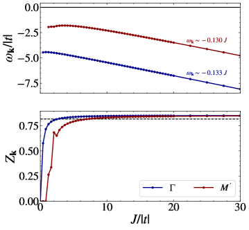
Figure 8: The polaron energy $\omega_{\mathbf{k}}$ (top panel) and quasi-particle residue $Z_{\mathbf{k}}$ (lower panel) as a function of $J/\absolutevalue{t}$ for $t>0$.

In the small to intermediate $J/\absolutevalue{t}$ regime the excited $M^{\prime}$ polaron state abruply disappears when $J/t\lesssim 1$. This sudden suppression of the quasi-particle weight has been analysed in detail in Ref. Trumper et al. (2004), using a similar approach but neglecting the static $J$-dependent spin-wave interaction. Our model reproduces their findings, altered by a small inflection point in the quasi-particle weight around the critical value.

Appendix E $J$ scaling of excited polaron modes

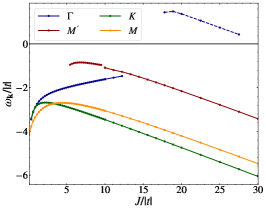
((a))

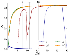
((b))

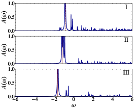
((c))

Figure 9: Behavior of the magnetic polaron in all four modes highlighted in Fig. 5 as a function of $J/\absolutevalue{t}$, for the case $t<0$. In Figs. (a) and (b) the polaron energy and spectral weight are shown, where each mode is distinguished with a unique colour. In Fig. (c) we show the full spectral function at the $M^{\prime}$ mode for three distinct values of $J$ encoded as points I, II and III. These are shown in Fig. (b) with vertical grey lines.

In this appendix we present some additional results for the scaling of the polaron modes with $J$, specifically considering the case $t<0$ and the scaling of the modes $\Gamma$ and $M^{\prime}$ in the inner parts of the BZ. Scans of the polaron energy and spectral weight similar to Fig. 7 in the main text are shown in Figs. 9(a) and 9(b).

Consider first the $M^{\prime}$ mode. As briefly mentioned in the main text, a robust quasi-particle solution already appears for intermediate value of $J$, although it does not develop smoothly into the coherent state. First around $J/\absolutevalue{t}\approx 10$ we observe a sharp feature in which the spectral weight of the polaron is strongly supressed. To understand this better we plot in Fig. 9(c) the full spectral function $A(\mathbf{\omega})$ at the $M^{\prime}$ mode for three different values of $J$ around the suppressive feature, denoted with I, II and III and also shown in Fig. 9(b). For $J/\absolutevalue{t}<10$ there exists a clear polaron solution as shown by the red dotted line. One will note that just below this peak there exist a couple of smaller resonances where $\absolutevalue{\omega_{\mathbf{k}}-\omega_{\mathbf{k}}^{\mathrm{h}}-\mathrm{Re}\Sigma(\mathbf{k},\omega_{\mathbf{k}})}$ has local minima. As $J$ is increased these minima move closer to zero, crossing through zero at some critical value of $J$ leading to new quasi-particle solutions just below the solution we have highlighted. At point II these different closely spaced solutions lead to a break-up of the quasi-particle peak, creating a strong suppression of spectral weight as observed in Fig. 9(b). As $J$ is increased further, a new single peak emerges that will subsequently develop into the coherent state, as shown in the spectral function at point III. The $\Gamma$ mode also shows different non-trivial behavior. For small and intermediate values of $J$ there exists a quasi-particle solution with low spectral weight, also observed in Ref. Trumper et al. (2004). As $J$ is increased this solution moves to higher energy, suggesting that it develops into some excited polaron state. Then at some point it is damped completely in favour of a new solution that quickly grows in spectral weight towards the asymptotic coherent state value. This solution however follows a similar curve as observed for the $M^{\prime}$ mode, with a strong suppression of spectral weight around $J/\absolutevalue{t}\approx 30$ before developing into the coherent state solution outside of the range we plot. Evidently the behavior of excited polaron modes in our model is quite complicated, and we note that it may be influenced by finite size effects that persist on our 1200 spin lattice.

Appendix F Comparison SCBA with large $J$ limit

In this appendix we show that the coherent state self-energy equation reproduces the SCBA equation up to first order in the dimensionless coefficient $\absolutevalue{\alpha_{\mathbf{k}}}=\absolutevalue*{V_{\mathbf{k}}^{J}/\omega_{\mathbf{k}}^{\mathrm{b}}}$. First we can use Eq. (13) to obtain the time dependent hole Green’s function $G(\tau)=-i\theta(\tau)\matrixelement*{h}{e^{-iH\tau}}{h}$. Using the same techniques as applied in deriving Eq. (20) we find,

$$\begin{split}G(\tau)=-i\theta(\tau)e^{-iE_{J}\tau}e^{-\sum_{\mathbf{k}}\absolutevalue*{\alpha_{\mathbf{k}}}^{2}\left(1-e^{-i\omega_{\mathbf{k}}^{\mathrm{b}}\tau}\right)}.\end{split}$$ (37)

Now take the derivative with respect to $\tau$ on both sides and Fourier transform to frequency space. Then we obtain the following self-consistent equation for the Green’s function,

$$\begin{split}G^{-1}(\omega)=\frac{\omega-E_{J}}{1+\sum_{\mathbf{k}}\frac{\absolutevalue*{V_{\mathbf{k}}^{J}}^{2}}{\omega_{\mathbf{k}}^{\mathrm{b}}}G_{\mathbf{r}}(\omega-\omega_{\mathbf{k}}^{\mathrm{b}})}.\end{split}$$ (38)

As expected the Green’s function diverges at the polaron ground state energy $\omega=E_{J}$, and is momentum independent. From the Green’s function we obtain a self-consistent equation for the self-energy,

$$\begin{split}\Sigma_{\mathbf{r}}(\omega)=\frac{\omega\sum_{\mathbf{k}}\frac{\absolutevalue{V_{\mathbf{k}}^{J}}^{2}}{\omega_{\mathbf{k}}^{\mathrm{b}}}\frac{1}{\omega-\omega_{\mathbf{k}}^{\mathrm{b}}-\Sigma(\omega-\omega_{\mathbf{k}}^{\mathrm{b}})}+E_{J}}{1+\sum_{\mathbf{k}}\frac{\absolutevalue{V_{\mathbf{k}}^{J}}^{2}}{\omega_{\mathbf{k}}^{\mathrm{b}}}\frac{1}{\omega-\omega_{\mathbf{k}}^{\mathrm{b}}-\Sigma(\omega-\omega_{\mathbf{k}}^{\mathrm{b}})}}.\end{split}$$ (39)

Note that for $V_{\mathbf{k}}^{J}=0$ this equation reduces trivially to the associated SCBA equation. A Taylor expansion to first order in $\alpha_{\mathbf{k}}$ gives,

$$\begin{split}\Sigma_{\mathbf{r}}(\omega)\approx\omega\sum_{\mathbf{k}}\frac{\absolutevalue{V_{\mathbf{k}}^{J}}^{2}}{\omega_{\mathbf{k}}^{\mathrm{b}}}\frac{1}{\omega-\omega_{\mathbf{k}}^{\mathrm{b}}-\Sigma(\omega-\omega_{\mathbf{k}}^{\mathrm{b}})}+E_{J}\end{split}$$ (40)

Or, upon substituting $E_{J}$ and rewriting,

$$\begin{split}\Sigma_{\mathbf{r}}(\omega)&\approx\sum_{\mathbf{k}}\frac{\absolutevalue{V_{\mathbf{k}}^{J}}^{2}}{\omega-\omega_{\mathbf{k}}^{\mathrm{b}}-\Sigma(\omega-\omega_{\mathbf{k}}^{\mathrm{b}})}\\ &\quad+\sum_{\mathbf{k}}\frac{\absolutevalue{V_{\mathbf{k}}^{J}}^{2}}{\omega_{\mathbf{k}}^{\mathrm{b}}}\frac{\Sigma(\omega-\omega_{\mathbf{k}}^{\mathrm{b}})}{\omega-\omega_{\mathbf{k}}^{\mathrm{b}}-\Sigma(\omega-\omega_{\mathbf{k}}^{\mathrm{b}})}.\end{split}$$ (41)

The first line is just the SCBA equation (30) with $t=0$. The second line encodes higher order corrections due to crossing diagrams neglected in the SCBA approach, which scale with higher powers of $\absolutevalue*{\alpha_{\mathbf{k}}}$.

References

- Anderson (1987) P. W. Anderson, Science 235, 1196 (1987).
- Lee et al. (2006) P. A. Lee, N. Nagaosa, and X.-G. Wen, Rev. Mod. Phys. 78, 17 (2006).
- Emery (1987) V. J. Emery, Phys. Rev. Lett. 58, 2794 (1987).
- Schrieffer et al. (1988) J. R. Schrieffer, X.-G. Wen, and S.-C. Zhang, Phys. Rev. Lett. 60, 944 (1988).
- Dagotto (1994) E. Dagotto, Rev. Mod. Phys. 66, 763 (1994).
- Anderson (1973) P. Anderson, Mater. Res. Bull. 8, 153 (1973).
- Szasz et al. (2020) A. Szasz, J. Motruk, M. P. Zaletel, and J. E. Moore, Phys. Rev. X 10, 021042 (2020).
- Capriotti et al. (1999) L. Capriotti, A. E. Trumper, and S. Sorella, Phys. Rev. Lett. 82, 3899 (1999).
- Zheng et al. (2006) W. Zheng, J. O. Fjærestad, R. R. P. Singh, R. H. McKenzie, and R. Coldea, Phys. Rev. B 74, 224420 (2006).
- White and Chernyshev (2007) S. R. White and A. L. Chernyshev, Phys. Rev. Lett. 99, 127004 (2007).
- Leung and Runge (1993) P. W. Leung and K. J. Runge, Phys. Rev. B 47, 5861 (1993).
- Chernyshev and Zhitomirsky (2009) A. L. Chernyshev and M. E. Zhitomirsky, Phys. Rev. B 79, 144416 (2009).
- Azzouz and Dombre (1996) M. Azzouz and T. Dombre, Phys. Rev. B 53, 402 (1996).
- Everts et al. (1998) W. Everts, H. Everts, and U. Körner, Eur. Phys. J. B 5, 317 (1998).
- Vojta (1999) M. Vojta, Phys. Rev. B 59, 6027 (1999).
- Srivastava and Singh (2005) P. Srivastava and A. Singh, Phys. Rev. B 72, 224409 (2005).
- Trumper et al. (2004) A. E. Trumper, C. J. Gazza, and L. O. Manuel, Phys. Rev. B 69, 184407 (2004).
- Shimizu et al. (2003) Y. Shimizu, K. Miyagawa, K. Kanoda, M. Maesato, and G. Saito, Phys. Rev. Lett. 91, 107001 (2003).
- Maśka et al. (2004) M. M. Maśka, M. Mierzejewski, B. Andrzejewski, M. L. Foo, R. J. Cava, and T. Klimczuk, Phys. Rev. B 70, 144516 (2004).
- Wang et al. (2004) Q.-H. Wang, D.-H. Lee, and P. A. Lee, Phys. Rev. B 69, 092504 (2004).
- Yamashita et al. (2008) S. Yamashita, Y. Nakazawa, M. Oguni, Y. Oshima, H. Nojiri, Y. Shimizu, K. Miyagawa, and K. Kanoda, Nature Physics 4, 459 (2008).
- Itou et al. (2008) T. Itou, A. Oyamada, S. Maegawa, M. Tamura, and R. Kato, Phys. Rev. B 77, 104413 (2008).
- Law and Lee (2017) K. T. Law and P. A. Lee, Proceedings of the National Academy of Sciences 114, 6996 (2017).
- Li et al. (2018) Y.-D. Li, Y. Shen, Y. Li, J. Zhao, and G. Chen, Phys. Rev. B 97, 125105 (2018).
- Ni et al. (2019) J. M. Ni, B. L. Pan, B. Q. Song, Y. Y. Huang, J. Y. Zeng, Y. J. Yu, E. J. Cheng, L. S. Wang, D. Z. Dai, R. Kato, and S. Y. Li, Phys. Rev. Lett. 123, 247204 (2019).
- Bourgeois-Hope et al. (2019) P. Bourgeois-Hope, F. Laliberté, E. Lefrançois, G. Grissonnanche, S. R. de Cotret, R. Gordon, S. Kitou, H. Sawa, H. Cui, R. Kato, L. Taillefer, and N. Doiron-Leyraud, Phys. Rev. X 9, 041051 (2019).
- Zhou et al. (2017) Y. Zhou, K. Kanoda, and T.-K. Ng, Rev. Mod. Phys. 89, 025003 (2017).
- Chiu et al. (2019) C. S. Chiu, G. Ji, A. Bohrdt, M. Xu, M. Knap, E. Demler, F. Grusdt, M. Greiner, and D. Greif, Science 365, 251 (2019).
- Brown et al. (2019) P. T. Brown, D. Mitra, E. Guardado-Sanchez, R. Nourafkan, A. Reymbaut, C.-D. Hébert, S. Bergeron, A.-M. S. Tremblay, J. Kokalj, D. A. Huse, P. Schauß, and W. S. Bakr, Science 363, 379 (2019).
- Koepsell et al. (2019) J. Koepsell, J. Vijayan, P. Sompet, F. Grusdt, T. A. Hilker, E. Demler, G. Salomon, I. Bloch, and C. Gross, Nature 572, 358 (2019).
- Ji et al. (2021) G. Ji, M. Xu, L. H. Kendrick, C. S. Chiu, J. C. Brüggenjürgen, D. Greif, A. Bohrdt, F. Grusdt, E. Demler, M. Lebrat, and M. Greiner, Phys. Rev. X 11, 021022 (2021).
- Koepsell et al. (2021) J. Koepsell, D. Bourgund, P. Sompet, S. Hirthe, A. Bohrdt, Y. Wang, F. Grusdt, E. Demler, G. Salomon, C. Gross, and I. Bloch, Science 374, 82 (2021).
- Yamamoto et al. (2020) R. Yamamoto, H. Ozawa, D. C. Nak, I. Nakamura, and T. Fukuhara, New Journal of Physics 22, 123028 (2020).
- Yang et al. (2021) J. Yang, L. Liu, J. Mongkolkiattichai, and P. Schauss, PRX Quantum 2, 020344 (2021).
- Cao et al. (2018) Y. Cao, V. Fatemi, S. Fang, K. Watanabe, T. Taniguchi, E. Kaxiras, and P. Jarillo-Herrero, Nature 556, 43 (2018).
- Tang et al. (2020) Y. Tang, L. Li, T. Li, Y. Xu, S. Liu, K. Barmak, K. Watanabe, T. Taniguchi, A. H. MacDonald, J. Shan, and K. F. Mak, Nature 579, 353 (2020).
- Balents et al. (2020) L. Balents, C. R. Dean, D. K. Efetov, and A. F. Young, Nature Physics 16, 725 (2020).
- Wu et al. (2018) F. Wu, T. Lovorn, E. Tutuc, and A. H. MacDonald, Phys. Rev. Lett. 121, 026402 (2018).
- Chao et al. (1977) K. A. Chao, J. Spalek, and A. M. Oles, J. Phys. C: Solid State Phys. 10, L271 (1977).
- MacDonald et al. (1988) A. H. MacDonald, S. M. Girvin, and D. Yoshioka, Phys. Rev. B 37, 9753 (1988).
- Eskes et al. (1994) H. Eskes, A. M. Oleś, M. B. J. Meinders, and W. Stephan, Phys. Rev. B 50, 17980 (1994).
- Schmitt-Rink et al. (1988) S. Schmitt-Rink, C. M. Varma, and A. E. Ruckenstein, Phys. Rev. Lett. 60, 2793 (1988).
- Kane et al. (1989) C. L. Kane, P. A. Lee, and N. Read, Phys. Rev. B 39, 6880 (1989).
- Martinez and Horsch (1991) G. Martinez and P. Horsch, Phys. Rev. B 44, 317 (1991).
- Liu and Manousakis (1991) Z. Liu and E. Manousakis, Phys. Rev. B 44, 2414 (1991).
- Nielsen et al. (2021) K. K. Nielsen, M. A. Bastarrachea-Magnani, T. Pohl, and G. M. Bruun, Phys. Rev. B 104, 155136 (2021).
- Mahan (2000) G. Mahan, Many-Particle Physics (Kluwer Academic/Plenum Publishers, 2000).
- Shashi et al. (2014) A. Shashi, F. Grusdt, D. A. Abanin, and E. Demler, Phys. Rev. A 89, 053617 (2014).
- Nielsen et al. (2022) K. K. Nielsen, T. Pohl, and G. M. Bruun, (2022), 10.48550/ARXIV.2203.04789.
- Manousakis (2007) E. Manousakis, Phys. Rev. B 75, 035106 (2007).
- Drescher et al. (2022) M. Drescher, L. Vanderstraeten, R. Moessner, and F. Pollmann, (2022), 10.48550/ARXIV.2209.03344.
- Browaeys and Lahaye (2020) A. Browaeys and T. Lahaye, Nature Physics 16, 132 (2020).