Pathfinding in Random Partially Observable Environments with Vision-Informed Deep Reinforcement Learning

Abstract

Deep reinforcement learning is a technique for solving problems in a variety of environments, ranging from Atari video games to stock trading. This method leverages deep neural network models to make decisions based on observations of a given environment with the goal of maximizing a reward function that can incorporate cost and rewards for reaching goals. With the aim of pathfinding, reward conditions can include reaching a specified target area along with costs for movement. In this work, multiple Deep Q-Network (DQN) agents are trained to operate in a partially observable environment with the goal of reaching a target zone in minimal travel time. The agent operates based on a visual representation of its surroundings, and thus has a restricted capability to observe the environment. A comparison between DQN, DQN-GRU, and DQN-LSTM is performed to examine each models capabilities with two different types of input. Through this evaluation, it is been shown that with equivalent training and analogous model architectures, a DQN model is able to outperform its recurrent counterparts.

Keywords— Reinforcment Learning, Deep Reinforcement Learning, Partially Observable Environment

1 Introduction

Deep Reinforcement Learning (DRL) has been applied to pathfinding in environments ranging from robot and drone operation [1, 2] to maritime navigation [3]. This technique has shown strong capabilities to create models that make intelligent decisions in these environments [3]. The DRL models are used to control entities acting in a given environment. These entities are referred to as “agents” [1]. Agents can utilize varying underlying deep learning models to make decisions, such as Multi-Layer Perceptron (MLP) [4], Recurrent Neural Networks (RNN) [1], Convolutional Neural Networks (CNN) [5], and others.

Optimal choice of the model depends on the information available in the target environment. For instance, in a fully observable environment, like a board game, a model with a memory capability is likely not necessary [4]. However, an agent operating in a partially observable environment can benefit from a model that has a recall capability, such as an RNN [1]. This class of environment can include scenarios such as autonomous vehicles and drones, certain classes of card games, and other instances where not all information pertinent to decision making is available at a given instant. In such environments, the decision making of a memory-capable neural network can benefit from past information [6].

Many works apply Reinforcement Learning (RL) to the problem of pathfinding in a variety of environments, where some of which are partially observable [1, 2, 3]. There are many instances where pathfinding must be achieved without complete knowledge of the environment. A prime example of this is vision-based navigation. In this case, an agent is set to search for a target in the environment based on visual input [7]. This leads to an inherently restricted observation space, as the agent is only able to see a portion of the environment from a given position. For instance, the agent will not be able to see a target that is behind it. In other instances, there can be obstacles included in the environment that may completely or partially occlude the agent’s view of the target.

Many works utilize a gridworld environment, where the agent learns to navigate an environment that is represented as a matrix of cells [2, 5, 8]. This enables path finding in realistic environments, but requires some overhead to translate the real environment into a grid world to make use of the model. Instead, by creating a training environment where the agent is informed based on depth vision, the trained agent is more ready to immediately operate in a realistic environment without the added translation into a grid world.

In this work, the modelled environment is treated as 2 dimensional and is partially observable to the agent. The agent’s vision consists of a label for the object in view, and the distance to it. This method can be readily expanded for application in a 3 dimensional environment, but by applying restricting the environment to 2 dimensions, the computational time needed to investigate this pathfinding problem are lowered to a more tractable level. The major contributions of this work are as follows:

• Design and implementation of an RL environment that expands the grid world environment concept for training models informed by depth-based visual information

• Design of a novel reward function to encourage effective training of RL models for pathfinding

• Training of RL models on randomized environment maps that are shown to be solvable with BFS and rising environment difficulty through a variable number of obstacles

• Performance comparison of three RL models during training and evaluation

• Examination of model performance when knowledge of the target location is known versus unknown

The remainder of this work is structured as follows: Section 2 contains a survey of related works, Section 3 describes the methods for environment generation for model training and evaluation. Section 4 describes the reinforcement learning configuration. Section 5 describes the model evaluation. Lastly, Section 6 concludes this work with a discussion of future expansion.

2 Background and Related Work

Panov et al. apply RL to the pathfinding problem using Q-learning [5]. In their work, the environment map is represented by a cell matrix, where each cell can be either traversible or have an obstacle. The agent is able to view a 5$\times 5$ section of the map. The agent is placed at the center of the 5$\times$5 portion. The work shows that the Q-learning method using a CNN for feature extraction is able to find valid paths in their partially observable environment [5].

In a work similar to Panov et al. [5], Peña and Banuti aim to evaluate reinforcement learning for pathfinding in environments with varying complexities [8]. Peña and Banuti use a modified version of the Open AI Frozen Lake environment, which is a 2D pathfinding environment that includes hazards to the agent, along with “slippery” tiles that introduce a random effect to agent actions within the environment. This work utilizes a limited observation space to examine the generalization ability of a Deep Q-Network (DQN) model. This is acheived by training the agent on a set of three maps, and evaluating its performance using unseen maps [8]. In contrast, this work utilizes camera-like vision to inform the model of the environment, and does not include random effects on the agent. Additionally, the training maps of this work are randomized so that the agent does not train on the same map twice.

Sartoretti et al. further expand the pathfinding problem to involve multiple agents [2]. Their work uses a gridworld in which the view is centered on each agent, similar to the previous two works. To avoid collisions between agents, the model is trained using a reward function that also penalizes collision heavily. Furthermore, selfish behavior is avoided by using a combination of RL and Imitation Learning to allow for an expert function to penalize agents for blocking the movement of other agents [2]. In contrast, this work does not investigate the multi-agent scenario.

Chen et al. implement a knowledge-free Q-learning model to plan paths for smart ships [3]. Faust et al. implement RL for probabilistic roadmaps, which aims to aid in long-range robot navigation using RL and sampling-based path planning [7]. Quan et al. use a recurrent double DQN architecture for robot path-planning in a gridworld environment [1]. Lastly, Sugimoto et al. examine the tracking capabilities of a DQN model [4]. These studies show applications of reinforcement learning to the path planning problem, but there are relatively few that utilize vision as input to the model, or that compare DQN models with recurrent versions as is done in this work.

3 The Seeker Environment

Algorithm 1 Gridworld Environment Generation

1:function GetEmptyCell($cells$)

2:    $x\leftarrow Random\>integer\>s.t.\>0\leq x<w$

3:    $y\leftarrow Random\>integer\>s.t.\>0\leq y<h$

4:    while $cells[y,x]\neq 0$ do $\triangleright$ Regenerate coordinates to get blank location as needed

5:       $x\leftarrow Random\>integer\>s.t.\>0\leq x<w$

6:       $y\leftarrow Random\>integer\>s.t.\>0\leq y<h$

7:    end while

8:    return $[x,y]$

9:end function

10:function EnvGeneration($w,h,o$)

11:    $cells\leftarrow h\times w\>\>zeroes$

12:    for $i\leftarrow 0:o$ do$\triangleright$ Generate Obstacle Locations

13:       $x,y\leftarrow GetEmptyCell(cells)$

14:       $cells[y,x]\leftarrow 1$$\triangleright$ Store obstacle location in matrix

15:    end for

16:    $x,y\leftarrow GetEmptyCell(cells)$

17:    $cells[y,x]\leftarrow 2$$\triangleright$ Store target location in matrix

18:    $x,y\leftarrow GetEmptyCell(cells)$

19:    $cells[y,x]\leftarrow 3$$\triangleright$ Store agent location in matrix

20:    return $cells$

21:end function

Many works utilize gridworld environments to evaluate RL pathfinding models. These environments are useful, but they are a restrictive abstraction of a realistic environment. To more closely model a real-world environment, in this work, a solvable gridworld map is generated. The solvable gridworld map is used to randomly generate the positions of the entities (agent, obstacles, and target). This map is then converted into a 2-dimensional plane, allowing for precise Euclidean distance measurements between two entities (any combination of agent, obstacles, and target). Instead of an obstacle being a cell in a matrix that the agent cannot move across, obstacles become 4-sided walls that block the forward movement of the agent. This forces the agent to operate by either turning or moving forward, allowing the output of the RL model to directly match actions that would be performed in a real environment. This reinforcement learning environment has been dubbed the “Seeker” environment.

------------   ------------   ------------   ------------   ------------ |          |   |        ! |   |    #     |   | ### # # !|   | @  #     | |          |   | @        |   |    ##    |   |# #   @#  |   | ## ## !# | |          |   |          |   |          |   |#         |   |#   ##  ##| |          |   |          |   |        # |   |  ##      |   | ##  #  # | |  @ !     |   |#         |   |          |   |    #     |   | # #      | |          |   |     #    |   | @ # !### |   |      ##  |   |  #   #  #| |          |   |      #   |   |      #   |   |     ###  |   | #  #  ## | |          |   |#       # |   | #        |   |##     #  |   | ##  ## ##| ------------   ------------   ------------   ------------   ------------

Figure 1: Example Random Gridworld Environments

To generate the gridworld, the EnvGeneration function from Algorithm 1 is used. This function takes the gridworld width, height, and the number of obstacles as input. Then, the GetEmptyCell function is used to find available positions via brute force to insert obstacles (Line 12-14) before inserting the agent (Line 19) and the target (Line 17) into their respective randomly selected cells. This yields environments such as those shown in Figure 1. The configured width of the shown maps is 10, and the height is 8. The “-” and “|” symbols represent the edges of the map, “@” is the agent, while “!” is the goal, and “#” represents an obstacle. The number of obstacles in the maps shown in Figure 1 varies from 0 to 30.

Algorithm 2 BFS for Verifying Goal Reachability

1:function CheckReacability($cells$,$x_{agent}$,$y_{agent}$,$x_{target}$,$y_{target}$)

2:    $w,h\leftarrow width(cells),height(cells)$

3:    $visited\leftarrow[[x_{agent},y_{agent}]]$

4:    $moves\leftarrow[[-1,0],[0,1],[1,0],[0,-1]]$ $\triangleright$ Left, Up, Right, Down $(x,y)$ move pairs

5:    while 1 do

6:       $visited.append([])$

7:       for $coor\in visited[-2]$ do $\triangleright$ For every cell visited in the last iteration,

8:          for $move\in moves$ do $\triangleright$ For every possible move from that cell

9:             $n\leftarrow coor+move$

10:             if $n_{x}>w$ or $n_{y}>h$ or $n_{x}<0$ or $n_{y}<0$ then $\triangleright$ Check that $n$ is within the gridworld

11:                continue

12:             end if

13:             $c\leftarrow cells[n_{y}][n_{x}]$

14:             if $c==$“!” then $\triangleright$ Target Found

15:                return True

16:             else if $c==$“ ” then $\triangleright$ Empty, Unvisited Cell Found

17:                append $n$ to $visited[-1]$

18:                $cells[n_{y}][n_{x}]==$“.”

19:             end if

20:          end for

21:       end for

22:       if $length(visited[-1])==0$ then $\triangleright$ Finding no empty cells in an iteration terminates the search

23:          return False

24:       end if

25:    end while

26:end function

Algorithm 2 demonstrates how Seeker uses Breadth-First Search (BFS) to check for goal reachability. Starting at the agent, all moves from the agent one cell in each cardinal direction (up, down, left, and right) are examined. If the target is found, “true” is returned. For any cell neighboring the agent, if they are empty, its position is noted in the $visited$ array, and its position in the $cells$ matrix is marked. Then, the sequence repeats, checking valid moves from the cells that were visited in the last iteration. This algorithm fills the cells matrix with “.” until it either finds the target or runs out of valid moves. Running out of valid cells to move to in an iteration indicates that the target is unreachable from the agent. This algorithm is a BFS because of the behavior of expanding the search outward from the agent. The purpose of the solvable gridworld map is to randomly generate the locations of the entities (agent, obstacles and target).

------- |     | |   # | |  # !| | @   | |   # | -------

(a)

------- | !   | |     | |  #  | |     | |  @  | -------

(b)

------- |   @ | |     | |###  | |     | |  !  | -------

(c)

Figure 2: Three example environments with their rendered 2D conversions and example agent views

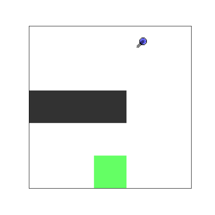
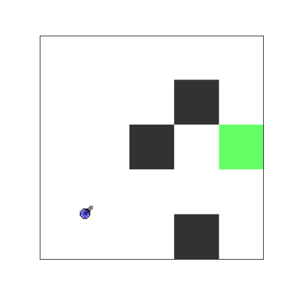
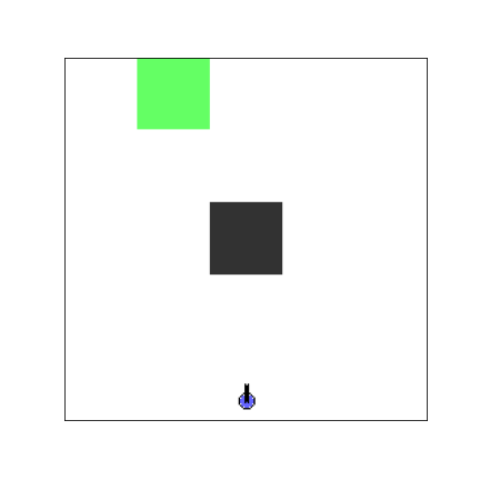
These randomly generated environments and entity positions are then converted to a 2D environment where the agent can move by turning or moving forward. This mimics how movement would occur in a realistic environment. Three examples of the environments after conversion along with the initial agent view are shown in Figure 2. In this figure, the target is rendered as a green box, while obstacles are black. The blue circle is the the agent. The direction it is viewing is indicated by the black tick extending from the blue circle. The agent is initialized to a random location within the cell specified by the “@” symbol in the gridworld map. The direction it is viewing is also randomly initialized.

4 Reinforcement Learning Configuration

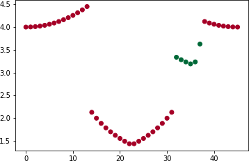
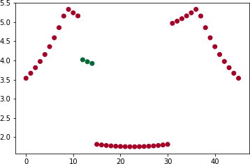
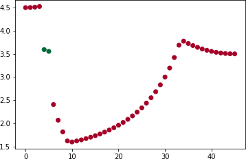
Using the view angle (the direction towards which the agent is facing) and location of the agent, a field of view (FOV) is defined that allows the agent to see the objects in front of it. This FOV is divided into slices, and for each slice, the distance from the agent to the object that the slice intersects with, along with the type of object, is found using a 2D ray-tracing algorithm. The type of the object is encoded as a 0 or a 1, where 1 is a target, and 0 denotes anything else, be it an obstacle or boundary. This trait is shown in Figure 2. In the bottom row of graphs, the height of the points from the $x$ axis denotes the distance from the agent to the object, and the color denotes the type of the object. The green colored points correspond to distances to the target, while red is a distance to a boundary or obstacle. This allows the agent to recognize that the boundary and obstacles should both be avoided in the same way.

Table 1: Reward Function used to train RL models

Condition	Reward
Near Obstacle	-1.0
Near Boundary	-1.0
Moved Away From Target	-1.5
Moved Toward Target	-0.2
Reached target	0.0
Default	-0.7

This view of the agent is used as input to the reinforcement learning models. The agent location, agent view angle, and the location of the center of the target are included as input for some models. Models that only receive the visual input are referred to as “Pure” models, whereas those that receive information on the location of the agent and the target are referred to as “Impure.” This distinction is made because the pure vision-based models will be required to seek the targets location in the environment, while the impure models will mainly need to learn how to avoid obstacles while approaching a known target.

The reward function used for training the RL models is manifold. First, if the agent is near an obstacle or boundary, there is a harsh penalty. Second, if the agent moves away from the target, the harshest penalty is applied, but moving toward the target applies a very low penalty. Reaching the target gives no penalty, and the last case is kept as default where a medium penalty is applied as a move cost. The values are shown in Table 1.

This reward function was designed to create a “punishment crater” centered on the target. Approaching the target applies low penalty, as if the agent is moving down a hill, but moving away increases the penalty sharply, similar to ascending a gradient. Being near an obstacle or the boundary is penalized sharply to encourage the agent to avoid them while it approaches the target.

The discount factor used is 0.99 for all time steps. When the agent reaches the target, a discount of 0.0 is given, as the episode has ended. This encourages the agent to consider rewards far in the future during decision making so that it can attempt to reach the goal as quickly and efficiently as possible during its search.

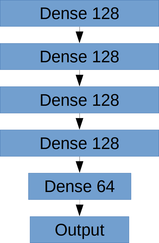
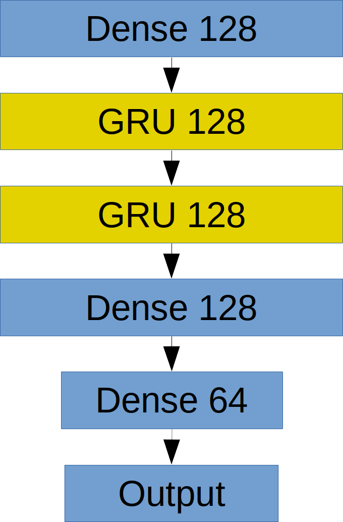
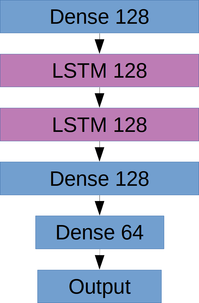
In total, six different models are trained and evaluated. They vary in the type of neural network used to construct the RL model and the input given to the model. First, a DQN is used, with only fully connected layers. The second model replaces the second two layers of the DQN with GRU layers. This changes the model into a DQRNN using GRU, hereafter referred to as the DQN-GRU. The third model replaces the GRU layers with LSTM cells. This model, similar to the second, is referred to as the DQN-LSTM. Each model uses a very similar architecture, to promote a fair comparison between them. Their architectures are shown in Figure 3. For each model architecture, models with both the pure and impure versions of input are trained and evaluated.

(a) DQN

(b) DQN-GRU

(c) DQN-LSTM

Figure 3: Architectures of the Evaluated RL models

Table 2: Discretized Actions

Discrete	Continous
	Move	Turn
0	0.05	-1
1	0.5	-0.5
2	1	0
3	0.5	0.5
4	0.05	1

These three models were chosen as they are all widely-used DNN and RNN methods. Furthermore, each model is expected to exhibit a different performance based on the design. While the DQN should handle an environment where the target is visible well, it will likely struggle when obstacles are introduced. On the other hand, the DQN-LSTM should have more memory power to handle more complex search environments. The DQN-GRU has a memory mechanism, but is less flexible than the DQN-LSTM, so it may not perform as well.

The Seeker environment receives action input as a pair of floating point values. The first element of this pair is the forward/backward movement. A positive value means that the agent should move forward, while a negative value corresponds to reverse movement. The magnitude of this value corresponds to the distance to be moved. The second element of the pair corresponds to left/right rotation of the agent. A negative value corresponds to a right turn, while positive values correspond to left. The magnitude of the value defines the amount the agent should turn. For this work, these actions are discretized into five integer numbered actions. These actions along with their corresponding move/turn pairs are shown in Table 2. Notice that reverse movement is disallowed, and all actions include at least a minimal forward movement component. This encourages the agent to always move, so that it can be exposed to the varying reward values, and make optimal decisions as it moves. Furthermore, in this environment, the agent does not need to stay in a fixed position. While rotation without movement may enable more optimal behavior, in terms of path length, removing this behavior enriches the variations of the reward function seen by the agent during the training process. This enrichment of the reward function enables a more efficient training process by preventing the model from choosing a behavior where it remains stationary. Instead, the model is forced to make an action, and therefore must learn to choose the optimal action.

Figure 4: Reward from Intermediate Evaluation During Training

5 Evaluation

Number of	Episode	Reward	Path
Obstacles	Length		Length
2	273.00	-165.80	4.89
4	263.45	-176.21	4.46
7	453.25	-288.17	6.66

(a) Pure DQN

Number of	Episode	Reward	Path
Obstacles	Length		Length
2	95.62	-51.20	3.04
4	117.46	-45.44	2.76
7	180.07	-60.28	3.35

(b) Impure DQN

Number of	Episode	Reward	Path
Obstacles	Length		Length
2	394.51	-340.93	5.39
4	373.63	-297.76	5.01
7	536.28	-428.15	6.70

(c) Pure DQN-GRU

Number of	Episode	Reward	Path
Obstacles	Length		Length
2	149.43	-87.40	3.05
4	176.04	-106.77	3.16
7	302.66	-157.27	3.87

(d) Impure DQN-GRU

Number of	Episode	Reward	Path
Obstacles	Length		Length
2	596.27	-435.83	4.76
4	527.01	-384.67	4.12
7	693.61	-567.16	5.02

(e) Pure DQN-LSTM

Number of	Episode	Reward	Path
Obstacles	Length		Length
2	308.71	-145.68	3.30
4	318.37	-147.90	3.25
7	441.67	-191.00	4.03

(f) Impure DQN-LSTM

Table 3: Average Evaluation Results for All Models

For evaluation, all six models were trained with the same random sequence of maps for the same number of time steps. The learning rate used was $1\times 10^{-5}$. First, each model is trained for 500k time steps in a sequence of maps without any obstacles; only the map boundary and target are present. Then, 3 obstacles are added before training for another 250k time steps. Last, a total of 5 obstacles are used for 250k time steps of training. This totals to 1 million time steps of training for each model. The number of episodes the model is exposed to is at least 1000, as the maximum length of an episode is 1000 time steps. However, due to the episodes being able to end early, the models may be exposed to more episodes depending on their learning capabilities. These increases in the number of obstacles present in the environment map allow for the agent to learn an easier version of the problem before it attempts to learn a more difficult version. This is done with the goal of training the models more quickly than if training was only performed in a difficult environment.

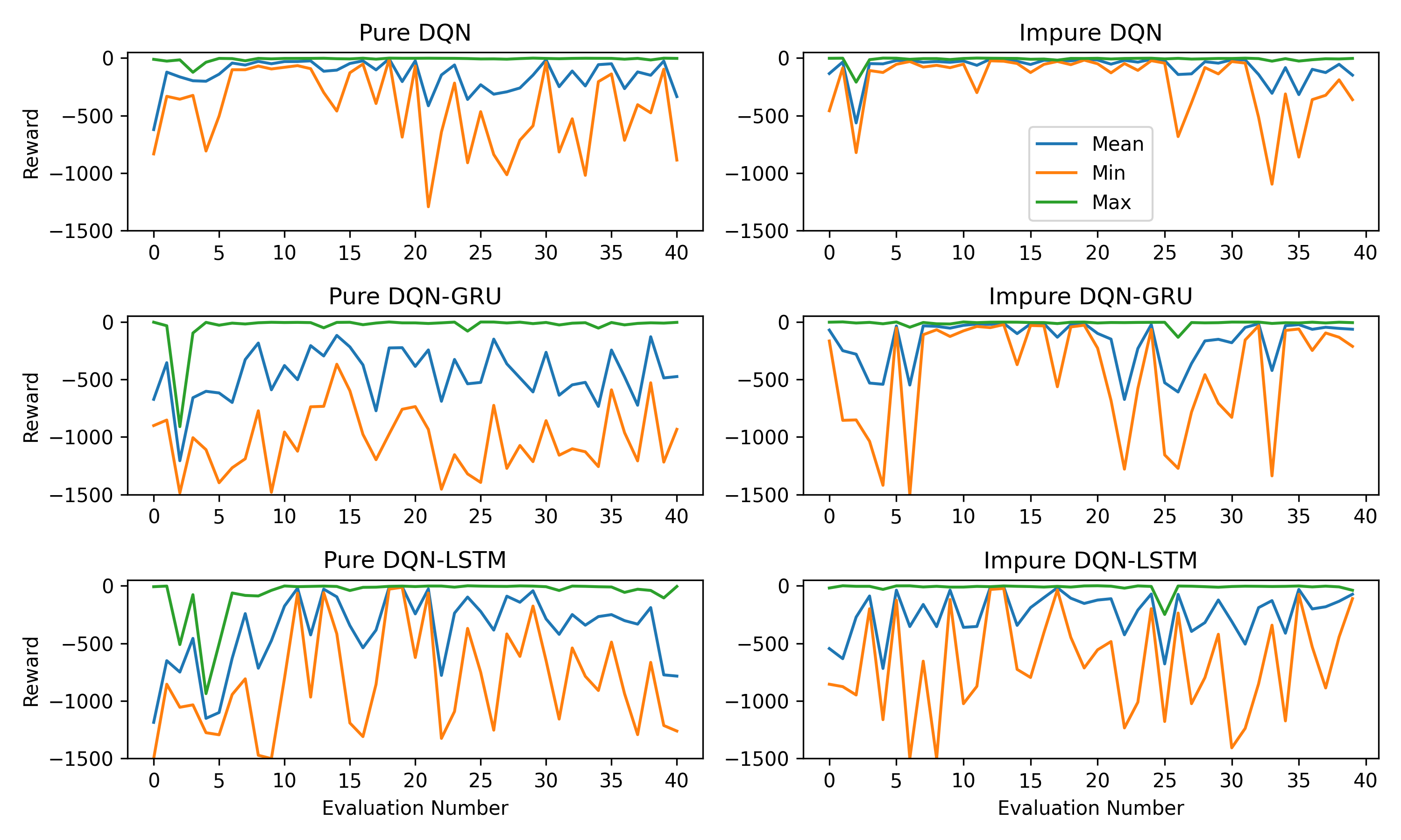
Each number of obstacles used during training defines a phase of training, meaning there are in total 3 phases of training. At every 25k time steps of training, training is halted to evaluate the models performance on a random set of 5 maps. So, for the first training stage, there are 20 evaluations, and for the second and third, 10 evaluations occur. This gives a view of how well the model has learned how to search for the target at that point in training. Figure 4 shows the results of this evaluation. Each row of the figure corresponds to a model architecture, while each column corresponds to the type of input used. The DQN models perform well when no obstacles are present, but cannot maintain their performance consistently as more obstacles are added. The Impure DQN-GRU model performs fairly well, and is able to learn how to handle obstacles much better than the DQNs were able to. Lastly, the DQN-LSTM model is shown. The impure version of model does fairly well, in terms of reward, but throughout training it is less stable than the DQN-GRU model, even if the average does tend to improve.

To thoroughly compare the capabilities of each of the three models, a set of tests are performed. Each model is tested using 2, 4, and 7 obstacles. These values are similar to the number of obstacles that are used during training, but 7 is higher than any that the agents see during training. This set of obstacle numbers allows for a comparison of the model performances when they are in environments similar to those used for training, along with a more difficult environment to examine each models generalization ability.

For each of the three chosen numbers of obstacles, each agent is evaluated in a sequence of 100 random environment maps. This sequence is the same for each agent. The average reward per episode, average episode length in time steps, and average agent path length are shown in Table 3. This evaluation shows that the DQN model is able to learn the environment much faster than the RNN versions, as the DQN tends to outperform the other models, especially in the impure case. Interestingly, however, the pure DQN-LSTM outperforms the pure DQN model in terms of the path length. The amount of time taken by the DQN-LSTM tends to be much higher than the DQN, and the reward is much lower, but it shows that it is able to find shorter paths to the target. This is likely due to the LSTMs capability to make better use of previously seen information when making decisions. The pure DQN-GRU model also has a memory capability, but it finds longer paths than either the DQN or DQN-LSTM model, and the pure DQN outperforms it in terms of episode length and reward.

6 Conclusion and Future Work

Pathfinding is a key problem for enabling autonomous robots, drones, and vehicles. Reinforcement learning provides a method to train models to perform pathfinding in a variety of environments, but many current research works focus on gridworld environments. These environments restrict the capability of the trained models, as any real world application of these models would need to rely on translation of the real environment into a grid. In this work, a simulated environment for training RL models named Seeker is introduced. The Seeker environment enables the training of models based on visual input to make realistic movement decisions. By informing models with vision, they are better prepared to be deployed in real world applications.

The evaluation performed in this work demonstrates the capabilities of three popular RL models in the Seeker environment, namely DQN, DQN-GRU, and DQN-LSTM. Each of these models utilizes a different mechanism for making decisions, and two have memory capabilities. Interestingly, the DQN model outperformed its recurrent counterparts when trained in an equivalent manner. This points to a need for differing training regimens for each model to obtain optimal performance.

Expansion of this work may include the addition of convolutional layers to the neural network models used. This addition will enable the extraction of learned spatial features from the vision, and potentially benefit the RL models’ capability to make decisions. Beyond this, there are many other RL models whose performance in this environment can be evaluated, both with discrete action sets and using the native continuous movement scheme. Furthermore, a thorough investigation into the recurrent models performance should be performed to determine the models optimal ability level in the Seeker environment.

References

- [1] H. Quan, Y. Li, and Y. Zhang, “A novel mobile robot navigation method based on deep reinforcement learning,” International Journal of Advanced Robotic Systems, vol. 17, no. 3, p. 1729881420921672, 2020.
- [2] G. Sartoretti, J. Kerr, Y. Shi, G. Wagner, T. S. Kumar, S. Koenig, and H. Choset, “Primal: Pathfinding via reinforcement and imitation multi-agent learning,” IEEE Robotics and Automation Letters, vol. 4, no. 3, pp. 2378–2385, 2019.
- [3] C. Chen, X.-Q. Chen, F. Ma, X.-J. Zeng, and J. Wang, “A knowledge-free path planning approach for smart ships based on reinforcement learning,” Ocean Engineering, vol. 189, p. 106299, 2019.
- [4] M. Sugimoto, R. Uchida, K. Kurashige, and S. Tsuzuki, “An experimental study for tracking ability of deep q-network,” International Journal of New Computer Architectures and their Applications, vol. 10, no. 3, pp. 32–38, 2021.
- [5] A. I. Panov, K. S. Yakovlev, and R. Suvorov, “Grid path planning with deep reinforcement learning: Preliminary results,” Procedia computer science, vol. 123, pp. 347–353, 2018.
- [6] S. Padakandla, “A survey of reinforcement learning algorithms for dynamically varying environments,” ACM Computing Surveys (CSUR), vol. 54, no. 6, pp. 1–25, 2021.
- [7] A. Faust, K. Oslund, O. Ramirez, A. Francis, L. Tapia, M. Fiser, and J. Davidson, “Prm-rl: Long-range robotic navigation tasks by combining reinforcement learning and sampling-based planning,” in 2018 IEEE International Conference on Robotics and Automation (ICRA), pp. 5113–5120, IEEE, 2018.
- [8] B. D. Pena and D. T. Banuti, “Reinforcement learning for pathfinding with restricted observation space in variable complexity environments,” in AIAA Scitech 2021 Forum, p. 1755, 2021.