Motion planning in task space
with Gromov-Hausdorff approximations

Abstract

Applications of industrial robotic manipulators such as cobots can require efficient online motion planning in environments that have a combination of static and non-static obstacles. Existing general purpose planning methods often produce poor quality solutions when available computation time is restricted, or fail to produce a solution entirely. We propose a new motion planning framework designed to operate in a user-defined task space, as opposed to the robot’s workspace, that intentionally trades off workspace generality for planning and execution time efficiency. Our framework automatically constructs trajectory libraries that are queried online, similar to previous methods that exploit offline computation. Importantly, our method also offers bounded suboptimality guarantees on trajectory length. The key idea is to establish approximate isometries known as $\epsilon$-Gromov-Hausdorff approximations such that points that are close by in task space are also close in configuration space. These bounding relations further imply that trajectories can be smoothly concatenated, which enables our framework to address batch-query scenarios where the objective is to find a minimum length sequence of trajectories that visit an unordered set of goals. We evaluate our framework in simulation with several kinematic configurations, including a manipulator mounted to a mobile base. Results demonstrate that our method achieves feasible real-time performance for practical applications and suggest interesting opportunities for extending its capabilities.

1 Introduction

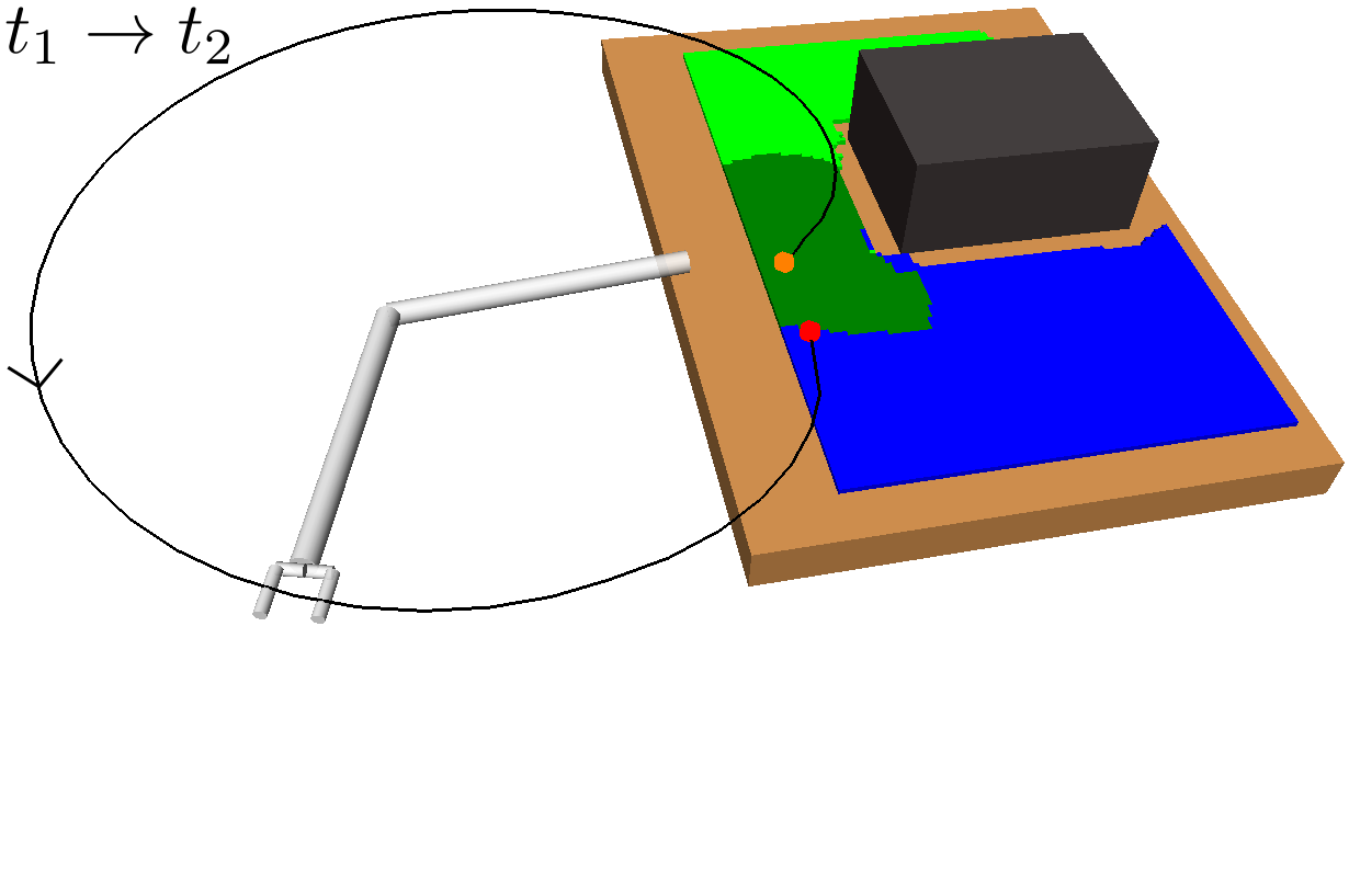
(a) Naive planner moving from first to second position

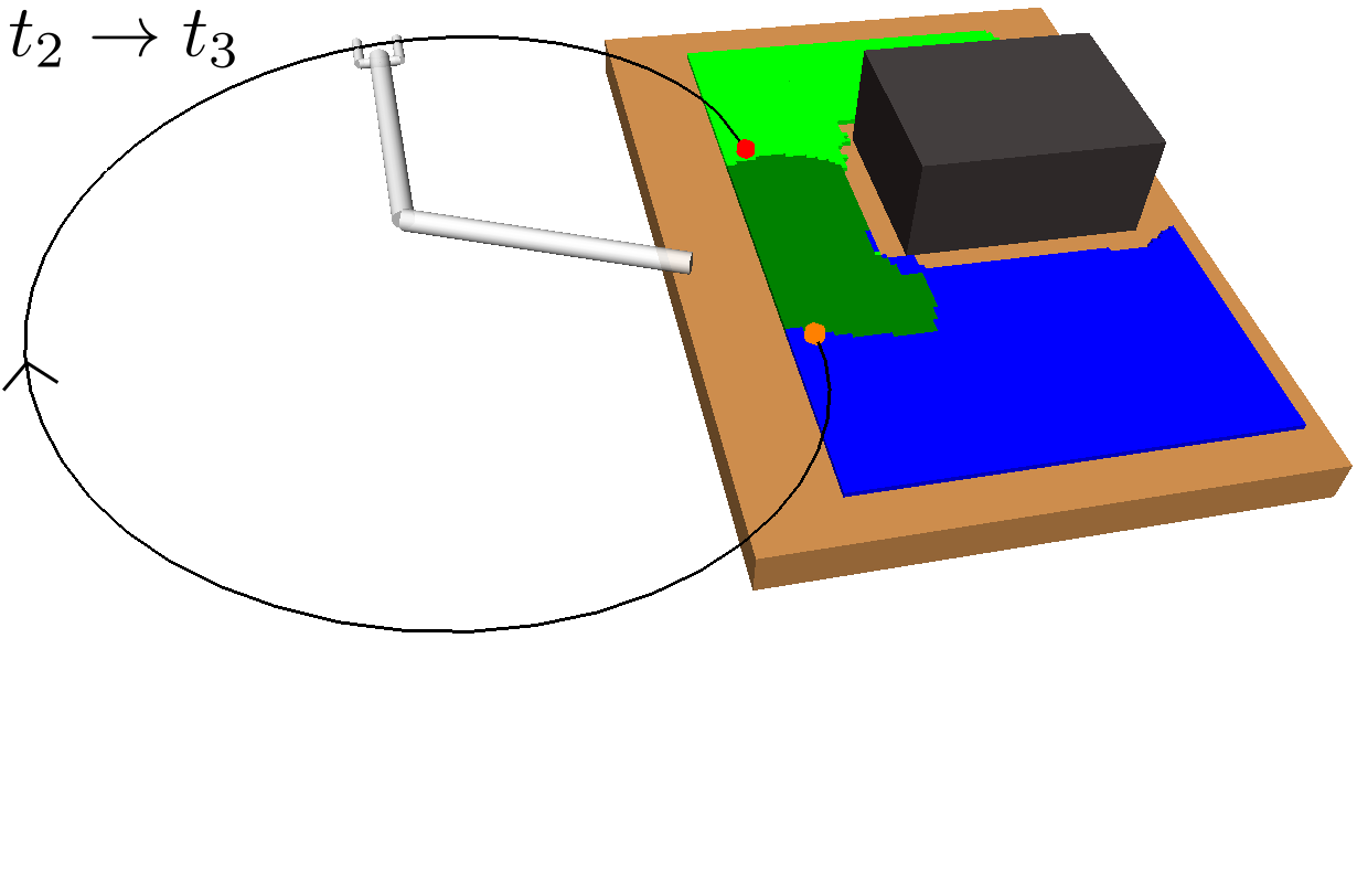
(b) Naive planner moving from second to third position

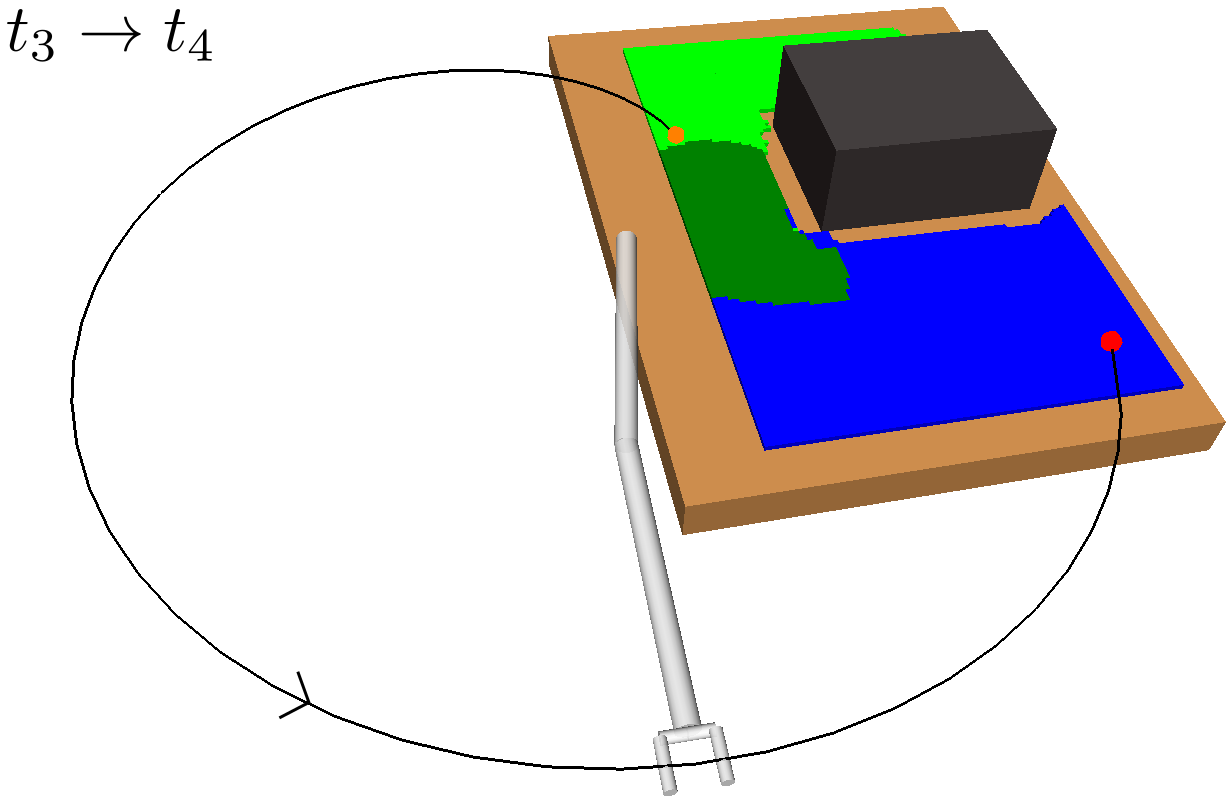
(c) Naive planner moving from third to fourth position

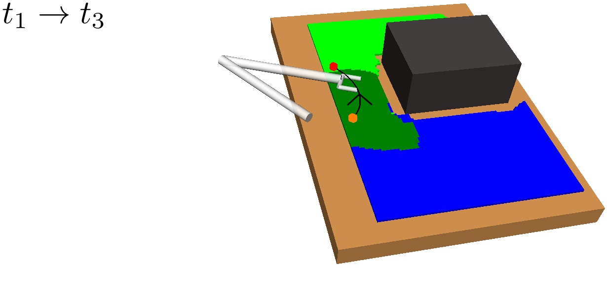
(d) HAP moving from first to third position

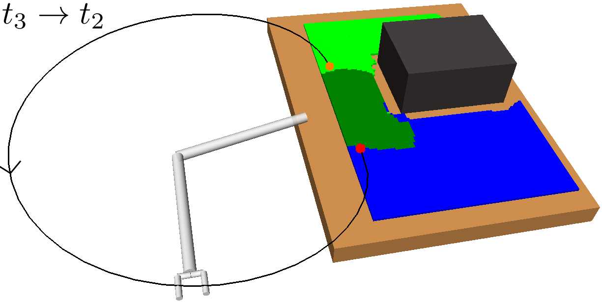
(e) HAP moving from third to second position

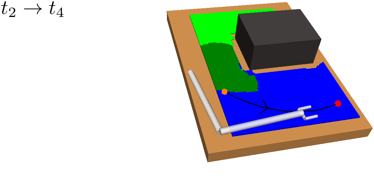
(f) HAP moving from second to fourth position

Figure 1: A two-DOF robotic manipulator tasked with moving its end effector to four unordered positions on a table-top environment with a box obstacle (dark grey). Positions are shown as coloured dots. The end-effector trajectory is drawn with direction of movement indicated by the arrowhead. Green and blue regions are subspaces within which end-effector motion does not require large changes in configuration. Overlap is shown in dark green. LABEL:sub@fig:task1_naive-LABEL:sub@fig:task3_naive show a sequence of trajectories produced by a naive planner. LABEL:sub@fig:task1_non_naive-LABEL:sub@fig:task3_non_naive show the sequence produced by our HAP method. HAP’s choice of sequencing exploits short within-subspace trajectories in LABEL:sub@fig:task1_non_naive and LABEL:sub@fig:task3_non_naive, whereas the naive planner’s choice of initial position and configuration results in long trajectories to satisfy kinematic constraints.

Motion planning for emerging applications of robotic manipulators must support a greater degree of autonomy than has traditionally been necessary. Industrial robotic manipulators such as cobots (collaborative robots), for example, are designed for advanced manufacturing applications where they should operate safely in dynamic work environments shared with humans and should be able to adapt quickly to perform a variety of tasks. These applications share a need for agility and rapid deployment that differs substantially from traditional applications of industrial manipulators, which are typically characterised by repetitive motions in highly structured environments with planning performed offline. Although existing motion planning algorithms have desirable computational properties such as probabilistic completeness, they are often limited in their ability to reliably produce feasible trajectories online in high-tempo tasks in practice.

We are interested in developing efficient algorithms for certain practical situations that require repeated, rapid, and reliable planning, including cobots and advanced manufacturing applications. A common example is a manipulator that must grasp objects from shelves and cabinets in a domestic or warehouse environment (srinivasa2012herb; dogar2013physics; morrison2018cartman). The shelves are static and their dimensions can be measured beforehand; however, the objects on the shelves might not be known and their locations can change. More precisely, we consider operational scenarios where a series of motion plans with differing goal configurations must be computed for a given environment. The environment consists of static elements such as fixtures and equipment plus potentially unknown objects that must be perceived online.

Classical approaches such as the probabilistic road map (PRM) (kavraki1996probabilistic) aim to gain efficiency through computational reuse; a computationally costly offline process generates a data structure that can then be repeatedly queried efficiently by a low-cost online process. However, this approach can become unwieldy in practice for robotic manipulators, which often have six or more degrees of freedom (DOF) and a configuration space of equivalent dimension. It is necessary to resolve the tradeoff between the size of the precomputed data structure, which grows naively with the complexity of the manipulator kinematics and environment, and the speed of online queries, whose complexity grows proportionally. Kinematic redundancy of robotic manipulators also introduces ambiguity in goal configuration when goals are specified only in terms of end-effector pose.

One way to limit the expanse of roadmap-like data structures, and thus improve query time, is through the notion of task space. Unlike configuration space and work space, which are defined by the physical design of the robot system, task space is defined by the user according to the tasks at hand (yu2018pid). An intuitive example is to define a planar task space for operations on a flat surface such as sanding or polishing. For pick-and-place operations, the task space can be naturally expressed as the set of end-effector poses that correspond to possible object locations. A set of trajectories can be generated that correspond to common start-goal locations, for example, and reused online (ellekilde2013motion; lee2014fast). Unfortunately, this approach requires substantial effort from the user since the set of precomputed trajectories must be designed for each set of tasks. It would be preferable to automate this process to allow the robot system to be redeployed quickly for new tasks and changes in the configuration of the environment, and to design the library of trajectories in a way that facilitates predictable execution online over long task horizons.

A desirable property of motion planning in task space is that, for any two tasks close to each other in task space, one expects a smooth, short trajectory to exist between them. The key idea we propose in this paper is to construct trajectory libraries that satisfy this property by establishing a bounding relation between distances in task space and corresponding distances in configuration space, defined as a mapping between metric spaces known as an $\epsilon$-Gromov-Hausdorff approximation ($\epsilon$-GHA). The aim is to ensure that a short path in task space implies a short path in configuration space, which additionally encourages smoothness.

We present the Hausdorff approximation planner (HAP) based on the key idea of constructing trajectory libraries with $\epsilon$-GHAs. HAP builds a set of precomputed trajectories that resemble roadmap methods in that trajectories can be concatenated to satisfy a sequence of queries as described in our motivating scenario. To allow concatenation, the trajectories are indexed by a set of maps from the task space (end-effector poses) to the configuration space (joint angles) that disambiguate kinematic redundancy. The maps are designed to be $\epsilon$-GHAs, which are approximate isometries that, as we show, ensure that the trajectories are efficient in combination. The task space is thus divided into smaller subspaces of similar manipulator configurations where, for any two poses close to each other in a given subspace, there exists a short trajectory between resulting configurations according to the map. As a result, each trajectory is efficient individually as well as in combination.

Given a user-defined task space, HAP automatically computes a subspace decomposition and generates a set of trajectories that span it. These trajectories are stored in a library that can be modified to adapt to changes in the environment or to the task-space definition. A simple illustration of two overlapping task subspaces that map to two disjoint configuration subspaces for a 2-DOF manipulator is shown in Fig. 1. As can be seen in the figure, a naive approach results in unnecessary wasted motion as opposed to our method which utilises the subspace knowledge. In higher dimensions, subspaces for 6-DOF or 7-DOF arms might differ in shoulder-in versus shoulder-out configurations, for example. Because only the task space itself is user-defined, this aspect of the algorithm’s design facilitates rapid deployment in practice.

We evaluate the behaviour of HAP in a single-query setting and then in a batch-query setting that requires it to find a minimum concatenated path through a set of unordered end-effector poses. The batch-query model could be used to take observations from a set of viewpoints with an eye-in-hand sensor, for example. To highlight HAP’s applicability to a variety of manipulator platforms and task-space definitions, we perform experiments in simulation with 6-DOF and 7-DOF manipulators, and with a manipulator mounted to a mobile base. Planning time performance is favourable overall, which shows that the HAP algorithm is effective in choosing precomputed trajectories for rapid online planning even in the presence of physical constraints, such as problematic singularities and joint limits, that otherwise would lead to unnecessarily long or awkward trajectories. Single-query results show a decrease in planning time of at least 50% versus baseline methods. Batch query results show a similar decrease in planning time and also a near perfect success rate with low jerk, whereas baseline methods failed to find a plan within the allocated time budget in at least 10% of problem instances.

The main significance of this work is to improve the practical utility of autonomous robotic manipulators, particularly for non-experts. Automatically generating smooth, short trajectories online directly from a user-defined task space with reasonable performance guarantees is a step beyond current general purpose motion planning methods, which generally require expertise to design implementations that perform well in practice. Our HAP implementation is made available as supplementary material.

2 Related work

2.1 Trajectory libraries

A variety of methods have been proposed that precompute a library of trajectories and adapt them online. For example, lin2016using utilise a trajectory library alongside a discrete planner for planning complex humanoid motions with palm contacts. Combining a trajectory library with a discrete planner is shown to improve planning success, particularly if the search space has a high branching factor.

A similar idea was explored by lee2014fast and ellekilde2013motion for robotic manipulators where a library of trajectories is precomputed over a roadmap of representative end-effector poses. These methods achieve lower online planning times, but exhibit inconsistent success rates and trajectory costs. This is partly because the online adaption does not consider collision avoidance. More importantly, these methods tend to ignore trajectory cost optimisation during library construction, which can lead to arbitrary performance when adapted online.

Our previous work (Sukkar2019; You2020) introduced a planning framework that builds on the ideas of lee2014fast and ellekilde2013motion and allows for non-static obstacles when adapting the library trajectories online. Library construction was designed to cover the entire task space with a single subspace, however, and we observed that this led to inconsistent performance that varied based on manipulator kinematics. Experiments with non-redundant 6-DOF manipulators were markedly less successful than with redundant 7-DOF manipulators, for example. We showed that coverage of the task space with a single subspace mapping was not possible and resulted in poorly biased trajectories for tasks outside of the mapped subspace.

The HAP framework we propose here resolves observed limitations of trajectory library methods by introducing the notion of organising task space as a set of multiple subspaces, and by providing bounded suboptimality guarantees through $\epsilon$-GHAs. In doing so, it allows for consistent performance across a variety of manipulator types, including non-redundant systems and mobile bases.

2.2 Trajectory optimisation

Trajectory optimisation generally refers to the process of making incremental changes to an initial trajectory until an optimal or near-optimal solution is found. The initial seed trajectory can be chosen randomly or heuristically. Existing methods can generate trajectories that avoid obstacles while maintaining smoothness (kalakrishnan2011stomp; park2012itomp; zucker2013chomp; schulman2014motion; mukadam2018continuous), and have been shown to be computationally efficient for high-dimensional systems (toussaint2009robot; zucker2013continuous; feng2015optimization).

The major limitation of trajectory optimisation methods is susceptibility to local minima, which leads to sensitivity to choice of initial trajectory. Initialisation has been shown to have a significant impact on convergence speed and success rate, and there is no guarantee of finding a collision-free solution as the collision avoidance constraints in the optimisation problem are non-convex (schulman2014motion).

A simple initialisation strategy is to draw a straight-line path between start and goal configurations in configuration space, ignoring obstacles. Others include attempts to learn classifiers that predict the effectiveness of random perturbations of a given seed trajectory (tallavajhula2016list; pan2014predicting; dey2013contextual). A recent learning-based approach (natarajan2021learning) uses long short-term memory (LSTM) neural networks, and exhibits better performance than straight-line initialisation.

The trajectory libraries constructed by HAP can be viewed as sets of high-quality seed trajectories that are precomputed based on manipulator kinematics and a priori knowledge of the environment. HAP uses trajectory optimisers to adapt these trajectories online.

2.3 Motion planning

General motion planning algorithms are the topic of decades of research. Good overviews can be found in textbooks (lavalle2006planning; choset2005principles) and surveys (elbanhawi2014sampling; gammell2020survey).

Sampling-based planners choose sample points from configuration space and connect them to build paths (kuffner2000rrt; kavraki1996probabilistic). Many variants have been proposed with a focus on probabilistic completeness and asymptotic optimality properties (karaman2011sampling; arslan2013use; gammell2014informed; janson2015fast). Batch Informed Trees (BIT*) (gammell2015batch; strub2020advanced) is a sampling-based algorithm that uses incremental search techniques to incorporate new samples. BIT* has been shown to perform well, in particular, for high-dimensional problems.

Recently, luna2020scalable proposed the XXL planner that computes high-quality trajectories for high-dimensional robots. XXL suffers from similar limitations as other sampling-based methods, however, and is probabilistically complete but offers no optimality guarantees.

Approaches for motion planning in task space, as we explore in this paper, are less common. shkolnik2009path proposed the TS-RRT algorithm, which is a modification of the RRT algorithm where samples are drawn from task space but connected in configuration space using techniques from task-space control. A benefit of this idea is that it avoids some of the challenges of sampling-based planning in high-dimensional configuration space, since task space is typically of lower dimension. For manipulators, this can also avoid the challenges of kinematic redundancy since paths in task space defined by end-effector pose are unique.

In order to satisfy the robot’s kinematic constraints, however, a path must still be found in configuration space. Short paths in task space are not necessarily so in configuration space, and so the challenge remains of how to mitigate the potentially large changes in joint configurations when attempting to connect the task-space samples. The work we present addresses this issue by establishing $\epsilon$-GHAs between the two spaces.

2.4 Task and motion planning

Task and motion planning (TAMP) problems extend motion planning to include high-level symbolic goals in a discrete action space (driess2020deep) and thus are different in character from the problems we address here. However, TAMP methods are related in their consideration of sequences of motion planning tasks. This consideration arises because a sequence of actions in the discrete layer must map to a sequence of motion plans in configuration space. Most TAMP approaches focus on feasibility of the task sequence as opposed to efficiency of the resulting concatenated trajectories (hauser2009integrating; srivastava2014combined; toussaint2015logic; garrett2018ffrob).

Work that considers properties of concatenated trajectories includes methods for task sequencing (alatartsev2013optimizing; kovacs2013task; kolakowska2014constraint; kovacs2016integrated) and multi-goal path planning (wurll2001point; faigl2011multi). Related methods often formulate the problem as a variant of the well-known travelling salesman problem (TSP) (alatartsev2015robotic). Unfortunately, these approaches are generally too computationally expensive for online use and require full knowledge in order for plans to be computed offline.

For online planning, it can be beneficial to use heuristics that accurately estimate true trajectory costs yet are efficient to compute within the process of solving the underlying TSP. Finding such a heuristic is difficult, however, without incurring computational cost equivalent to solving the original motion planning problem (hauerdeformable).

Heuristics for manipulators typically approximate trajectory costs by using Euclidean distance between start and goal points in the workspace (apple_2017; bac2017performance). This type of approximation can dramatically underestimate the true cost of the executed trajectory due to the nonlinearity of high-dimensional manipulators (fredsmp), especially in environments with obstacles.

The trajectory libraries proposed here provide accurate costs that take into consideration the kinematic redundancy and nonlinear motion model of high-dimensional manipulators, and allow trajectories to be smoothly concatenated. Therefore, they can be used as efficient heuristics for task sequencing, as we demonstrate.

3 Problem formulation and approach

3.1 Notation

$\mathcal{C}$ represents the configuration space of the arm. The workspace, $W$, is the 3D Euclidean workspace, $W=\mathbb{R}^{3}$. Given a configuration $q\in\mathcal{C}$, $A(q)\subset W$ denotes the space occupied by the robot model at configuration $q$. $m\subset\mathbb{R}^{3}$ is an approximate model of the environmental obstacles. We assume access to a collision checking process that reports whether the arm is in collision with $m$ or with itself. The obstacle region is defined as $\mathcal{C}_{\text{obs}}=\{q\in\mathcal{C}\mid A(q)\cap m\neq\emptyset\}$, from which we obtain the free space region $\mathcal{C}_{\text{free}}=\mathcal{C}\setminus\mathcal{C}_{\text{obs}}$. A task $t$ typically has a set of inverse kinematics (IK) solutions $\mathcal{Q}(t)$. Then, the task space $\mathcal{T}\subset SE(3)$ is the set of poses of the robot’s end effector for which valid IK solutions, $Q(t)\subset\mathcal{Q}(t)$ exist. An IK solution $q$ is considered valid if $A(q)\in\mathcal{C}_{\text{free}}$. $\hat{T}$ is a discrete approximation of the subset of $\mathcal{T}$ where the robot is expected to operate frequently.

3.2 Motion planning in task space: single-query problems

The manipulator is given a task modelled as a 6D pose $t\subset\mathcal{T}$ chosen from the task space. To complete the task, the manipulator must position its end effector at pose $t$ while avoiding collision. The environment is not entirely known in advance, but a general model $m$ is available that approximates what is expected. For example, $m$ might represent a general bookshelf structure including the shelves and case (see Fig. 2). However, $m$ need not include all objects within the bookshelf, as these details may be unknown a priori and discovered later.

The manipulator’s trajectory is modelled as a discrete sequence of configurations $\pi=\{\pi[1],\ldots,\pi[N]\mid\pi[i]\in\mathcal{C}_{\text{free}}\}$. We measure the length of a trajectory using a metric on the configuration space,

$$d_{C}(\pi)=\sum_{n=1}^{N-1}d_{C}(\pi[n],\pi[n+1]).$$ (1)

We are interested in finding a minimum cost trajectory in $\mathcal{C}_{\text{free}}$ that completes task $t$. It is convenient to consider the starting pose of the end effector to be the goal pose of the previous task. We are therefore interested in the set of trajectories between task $t_{j}$ and $t_{l}$, $\Pi(t_{j},t_{l})=\{\pi\mid\pi[1]\in Q(t_{j}),\pi[N]\in Q(t_{l})\}$, leading to the following problem definition.

Problem 1 (Motion planning in task space [single query]).

Find the shortest collision-free path $\pi^{*}$ in configuration space between two tasks $t_{j}$ and $t_{l}$ in $\mathcal{T}$ such that

$$\pi^{*}(t_{j},t_{l})=\operatorname*{arg\,min}_{\pi\in\Pi(t_{j},t_{l})}d_{C}(\pi).$$ (2)

3.3 Motion planning with multiple tasks: batch-query problems

The operational scenarios that motivate this work often involve more than one task. The manipulator is given an unordered set of $M$ tasks $T=\{t_{i}\}_{i=1}^{M}\subset\mathcal{T}$. This set of tasks can be viewed as a batch-query scenario where all tasks must be achieved while minimising total cost. Thus it is necessary to choose a sequence of tasks, imposing a total ordering over $T$, in addition to repeatedly solving Problem 1. The batch-query problem can thus be formulated as follows.

Problem 2 (Motion planning in task space [batch query]).

Find a permutation of the tasks $\sigma\in S_{M}$ that minimizes the total trajectory cost:

$$\min_{\sigma\in S_{M}}\sum_{n=1}^{M-1}d_{C}(\pi^{*}(t_{\sigma[n]},t_{\sigma[n+1]})),$$ (3)

such that the configuration at the end of $\pi^{*}(t_{\sigma[n]},t_{\sigma[n+1]})$ and the start of $\pi^{*}(t_{\sigma[n+1]},t_{\sigma[n+2]})$ are equal for all $n\in[1,M-2]$.

It is challenging to approach this case directly. For each task pose $t_{j}\in T$ to be visited, there can be multiple valid configurations in set $Q(t_{j})$. A direct solution requires simultaneously choosing the optimal configuration from $Q(t_{j})$ and sequencing the tasks. In other words, this case contains an instance of set-TSP, which is more difficult than the standard TSP (noon1993efficient) and potentially too computationally expensive for real-time planning since the number of possible sequences is $\mathcal{O}(|Q(t_{j})|^{M}\times M!)$, where $|Q(t_{j})|$ is the cardinality of the largest set of IK solutions for any task $t_{j}\in T$.

Mapping each task $t_{j}$ to a single IK solution $q_{t_{j}}\in Q(t_{j})$ transforms the set-TSP to a classical TSP, which is easier to solve. However, intelligent selection of a single IK solution from the possibly infinite set is also challenging.

Ideally, this transformation should accommodate efficient solution of Problem 1 with smooth, short trajectories between tasks. Therefore, we assume the availability of a mapping from each task $t_{j}$ to a suitable unique IK solution $\theta(t_{j})\in Q(t_{j})$. Finding such a mapping thus arises as an important subproblem in our approach to solving Problem 2 and is defined as follows.

Problem 2.1 (Mapping from task space to configuration space).

Find map $\theta:\hat{T}\to\mathcal{C}$ that assigns each task a unique IK solution that guarantees paths between tasks are short, smooth and collision-free in both task and configuration space.

The kinematics of a robotic manipulator working in the task space may not necessarily admit a single map $\theta$ with the guarantee above. For example, in Fig. 1a there is no single $\theta$ that allows the arm to travel the short task-space distance required without taking a long path through configuration space. To handle such cases, we propose a further subproblem crucial to solving the problems presented above.

Problem 2.2 (Finding regions of short travel in both task and configuration space).

Find $K$ subspaces $\{\hat{T}^{i}\}_{i=1}^{K}$ of task space such that within each subspace a map $\theta^{i}:\hat{T}^{i}\rightarrow\mathcal{C}^{i}$ that satisfies the requirements in Problem 2.1 can be found.

3.4 Approach overview

To ensure that the map $\theta:\hat{T}\to\mathcal{C}$ solves Problem 2.1, it is chosen to be an approximate isometry. Intuitively, an approximate isometry enforces that two tasks close in task space remain close in configuration space after mapping. Where a single approximate isometry does not exist, Problem 2.2 is solved by finding $K$ approximate isometries. This decomposes the task space into subspaces that may overlap, leading to cases where a single task is assigned multiple IK solutions. Then, to solve Problem 2 we find solutions within each subspace independently after disambiguating which IK solution to use in overlapping subspace regions.

We construct the map(s) $\{\theta\}_{i=1}^{K}$ offline during the process of building a library of pre-computed trajectories tailored to the given task space. This library is made available to online algorithms designed to solve both types of query problems. Together, the offline and online algorithms form the HAP algorithmic framework.

4 Online motion planning with task subspaces

In this section, we present online algorithms to solve Problems 1 and 2. We first describe methods to retrieve, modify, and adapt trajectories drawn from the library in the single-query case. Then, we describe several additional steps necessary to address the batch-query case through task sequencing.

4.1 Trajectory retrieval and adaptation for single-query problems

Given a task drawn from the task space $T$, we must first identify matching tasks in the trajectory library constructed from a discrete set of anticipatory tasks $\hat{T}$ and retrieve corresponding trajectories. Examples of $\hat{T}$ and online tasks $T$ are shown in Fig. 2. A retrieved trajectory is then modified such that its start and endpoints coincide with the current end-effector pose and that of the given task. These processes are summarised in Alg. 1 and detailed below.

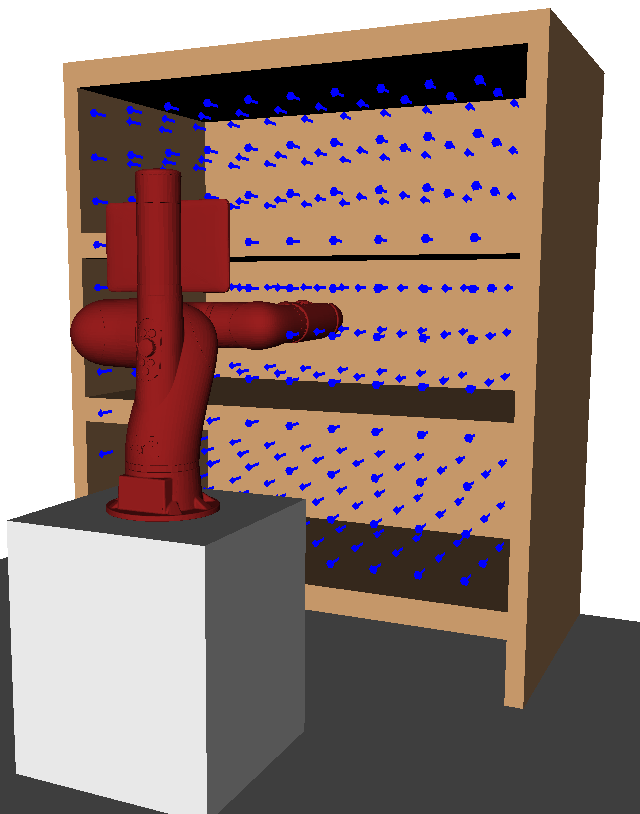
(a)

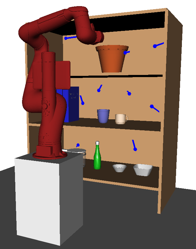
(b)

Figure 2: Example environment and task space next to an anticipated online scenario: LABEL:sub@fig:offline_grid shows the discretised task space $\hat{T}$ (blue poses) and inflated environment $m$, LABEL:sub@fig:online_scenario is an example online scenario with the arm in its home configuration. Online, HAP is robust against objects in LABEL:sub@fig:online_scenario that are unmodelled in $m$ and tasks can differ to those in $\hat{T}$.

Algorithm 1 Online Planner: Single Query

1:Given an online environment and task, retrieve matching library trajectories (Sec. 4.1.1)

2:Disambiguate IK solution (Sec. 4.1.2)

3:Augment chosen trajectory by appending start and goal configurations (Sec. 4.1.3)

4:Adapt trajectories to online environment (Sec. 4.2)

4.1.1 Trajectory library matching

Here we describe the library retrieval process where a single map $\theta$ is sufficient to solve Problem 2. Additional steps taken for the multiple map case are given in the next subsection. The trajectory library can be queried to retrieve a trajectory that connects a given pair of tasks drawn from the task space. We refer to endpoints of all such trajectories as library tasks, i.e., tasks stored within the library. Throughout this work, we assume that the task space is defined over the set of end-effector poses and thus the term task can be assumed to refer to one such pose.

The library allows for retrieval of trajectories whose start and endpoints lie close to a given pair of online tasks. We now describe the process of evaluating such trajectories to choose the best match.

Given an online task $t$, we query the library to find a set of library tasks near $t$. We select the $k$-closest $\{\hat{t}_{n}\}_{n=1}^{k}\subset\hat{T}$ to $t$ according to task-space distance. The task-space distance metric is user defined; here we use Euclidean distance between position components. To facilitate search, the library builds a KD-tree over task positions using this metric.

For the set of $k$-closest candidates, we retrieve their IK solutions assigned by $\theta$, $\{\theta(\hat{t}_{n})\}_{n=1}^{k}$, and compare them pairwise to all possible IK solutions $q_{t}\in Q(t)$ for task $t$ using a suitable similarity metric in configuration space. We use the $L_{2}$-norm in this work. The pair of online/library task configurations $(q_{t}^{*},\theta(\hat{t}_{*}))$ that minimises this metric is selected as a match.

HAP’s matching process is different from previous work in that it depends on both task and configuration-space distances, rather than configuration-space distance alone (lee2014fast; ellekilde2013motion). Whereas configuration-space distance favours IK solutions that result in the least joint movement, task-space distance restricts the matching process to reflect the workspace geometry. To elucidate this claim, consider the bookshelf environment in Fig. 2. If matching is performed to minimise configuration-space distance only, an online task located in the middle shelf may be matched with a library task in the top shelf due to the small configuration change between them. Then, appending the online task to any retrieved trajectory corresponding to the top shelf library task would result in collision. On the other hand, if matching is performed to minimise task-space distance only, a matched library task is more likely to lie in the middle section of the bookshelf since shelf geometry is taken into account yet may result in inefficient, jerky trajectories due to potentially large differences in configuration space.

4.1.2 Subspace assignment

During construction of the library, all tasks $\hat{t}\in\hat{T}$ are mapped to an IK solution by finding approximate isometry or isometries $\{\theta\}_{i=1}^{K}$. It is possible for these mappings to overlap, resulting in multiple IK solutions for a given task (one per map). Examples of the benefit of multiple mappings are given in Appendix LABEL:fig:reachable_comparison.

To handle the case where a library query results in multiple IK solutions due to overlapping mappings, it is necessary to define a process to choose one of them. It suffices to compare candidate IK solutions to the current robot configuration using the similarity metric discussed above (e.g., the $L_{2}$-norm in configuration space) and select the minimum. For computational efficiency, we select the first candidate whose similarity value falls below a given threshold.

The final special case to consider is one where the start and goal poses lie in disjoint mappings, and thus no trajectory exists in the library that connects them. To handle this case, a home configuration for the robot is defined in the library. The home configuration is chosen by the library construction procedure such that all subspaces may be reached via a straight-line trajectory in configuration space. Thus the home configuration acts as an intermediate point connecting all pairs of subspaces, and can be used to connect start and goal poses in disjoint mappings by simply joining the straight line trajectories to and from it.

4.1.3 Trajectory modification

The matching trajectory chosen from the library will not align exactly with the start and goal poses of the robot in practical use. In general it is necessary for the library to be compact relative to task space in order to limit required storage to an acceptable level.

For start and goal poses $(t_{j},t_{l})$, the corresponding IK solutions $q_{t_{j}}^{*}$ and $q_{t_{l}}^{*}$ are appended to the ends of the retrieved library trajectory. This results in a modified trajectory $\pi^{*}(t_{j},t_{l})$ which connects $t_{j}$ and $t_{l}$.

4.2 Online adaptation

The final algorithmic step before a trajectory can be executed by the robot is to perform post-processing to ensure that it is time-continuous safe, i.e., that it lies entirely within $\mathcal{C}_{\text{free}}$. Although the library is constructed such that its trajectories avoid known obstacles, this step is crucial for robustness against obstacles that were unknown during library generation. We refer to this post-processing as adaptation.

There are a number of existing trajectory optimisation algorithms that are designed for similar purposes. In general, these algorithms require an initial seed trajectory as input, which they attempt to adapt to satisfy given constraints and maximise/minimise a given objective. In this work we use the TrajOpt (schulman2014motion) algorithm with the modified library trajectory used as the seed trajectory.

Unfortunately, TrajOpt and similar trajectory optimisation approaches are not guaranteed to succeed in finding a solution and depend heavily on the choice of seed trajectory. The modified library trajectory already accounts for obstacles known at the time of library construction and is preferable to less informed choices, such as a straight line trajectory in configuration space. However, a fallback method remains necessary in case of failure due to obstacles discovered at execution time. The fallback method should be guaranteed to find a solution, since it is a method of last resort. HAP uses BIT* (gammell2015batch), a well-known probabilistically complete planner, with the IK solution defined in the modified library trajectory used as its goal configuration input. Like all probabilistically complete methods, BIT* may fail to find a solution in a reasonable amount of time. HAP enforces a user-defined threshold and terminates execution if exceeded. This is the only condition in which HAP fails to produce an executable trajectory.

4.3 Additional operations for task sequencing in batch-query problems

Algorithm 2 Online Planner: Batch Query

1:Given an online environment and set of tasks, group tasks by subspace

2:Append home configuration to each group

3:Execute Lines 1–3 of Alg. 1 for each pair of tasks within each group

4:Construct weighted adjacency matrix for each group, using computed trajectory costs as weights

5:Compute optimal sequence for each group using TSP solver with associated weight matrix and start/end constrained to home configuration

6:Concatenate sequences

7:Execute Line 4 of Alg. 1 for each successive pair of tasks in the concatenated sequence

The batch-query case is addressed by introducing several additional steps in Alg. 2. Given a set of online tasks $T$, we group tasks by subspace and describe how the single-query processes just described are used to find a minimal sequence of trajectories between them.

Each task $t\in T$ is assigned to one of the subspace mappings $\theta^{i}$ by querying the library. The tasks are partitioned into groups of equivalent subspace assignment, and the home configuration is appended to each group. The single-query process is then executed for all pairs of tasks within each group. The trajectory costs returned are stored as a weighted adjacency matrix. Thus each task group has an associated matrix where the weights correspond to the trajectory cost for each pair of tasks within the group, including the home configuration. These matrices are used as input to a TSP solver, which returns a task sequence for each group independently. The TSP solver is constrained such that each sequence begins and ends at the home configuration.

The sequences are concatenated in arbitrary order. This concatenation is always possible by construction of the sequences, which all start and end at the home configuration. Finally, the online adaptation process is executed for each pair of tasks in the concatenated sequence and the result is returned.

5 Trajectory library construction

In this section we detail how the maps $\{\theta^{i}\}_{i=1}^{K}$ and trajectory library are computed given a robotic manipulator, anticipated environment, and task space. Additionally, practical considerations are given that describe implementation specific details useful when applying HAP.

5.1 Algorithm overview

To construct the trajectory library, we are given an anticipated environment $m$ and set of tasks $\hat{T}$ that are representative of online scenarios. An undirected graph $G$ is created with nodes corresponding to tasks $t\in\hat{T}$ and edges formed via a maximum connection radius (see Sec. LABEL:sec:practical:graph). Figure 3 shows an example $G$ constructed over the $m$ and $\hat{T}$ in Fig. 2LABEL:sub@fig:offline_grid. The trajectory library is then generated from $G$ according to Alg. 3.

Algorithm 3 is initialised by assigning all nodes to $\hat{T}_{\text{open}}$. A node stays in $\hat{T}_{\text{open}}$ until a unique IK solution is assigned. While $\hat{T}_{\text{open}}$ is not empty, $\theta$ is found via a generate map algorithm procedure (Alg. 4). Algorithm 4 searches for a $\theta$ that minimizes the objective cost, the sum of all minimum cost paths $\pi^{*}(t_{0},-)$ from a root node $t_{0}\in G$ to all other nodes. That is,

$$J(\theta,t_{0})=\sum_{t\in G\setminus t_{0}}g(\pi^{*}(t_{0},t);\theta),$$ (4)

where the cost of any path $\pi(t_{0},t_{N-1})=\{\theta(t_{0}),\ldots,\theta(t_{N-1})\}$ of $N$ nodes is defined as

$$g(\pi(t_{0},t_{N-1});\theta)=\sum_{n=0}^{N-2}d_{C}(\theta(t_{n}),\theta(t_{n+1})).$$ (5)

To ensure that trajectories have bounded lengths and do not involve large, unnecessary arm movements, $\theta$ is additionally constrained such that it is an approximate isometry, or an $\epsilon$-Gromov-Hausdorff approximation ($\epsilon$-GHA), defined below.

Definition 1.

The map $\theta:(\hat{T},d_{T})\to(\mathcal{C},d_{C})$ is an $\epsilon$-Gromov-Hausdorff approximation if $\forall t_{j},t_{l}\in\hat{T}$

$$|d_{T}(t_{j},t_{l})-d_{C}(\theta(t_{j}),\theta(t_{l}))|<\epsilon$$ (6)

for some $\epsilon>0$.

Depending on the value of $\epsilon$, topology of $m$ and robot kinematic structure, some nodes may still have undefined mappings after a single iteration of the algorithm. It may then be necessary to search for multiple $\epsilon$-GHAs, $\{\theta^{i}\}_{i=1}^{K}$, that map a covering set of subspaces $\{\hat{T}^{i}\}_{i=1}^{K}\subset\hat{T}$ to a set of disjoint subspaces $\{\mathcal{C}^{i}\}_{i=1}^{K}\subset\mathcal{C}$. After the $\epsilon$-GHA(s) is (are) found, we use the Dijkstra’s algorithm to find minimum cost paths $\pi^{*}(t_{j},t_{l})$ pairwise between all tasks $t_{j},t_{l}\in G$ using the fixed, unique IK solutions assigned by $\theta$ or $\{\theta^{i}\}_{i=1}^{K}$. The minimum cost paths are then stored in the trajectory library.

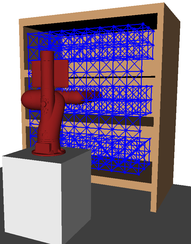
Figure 3: An undirected graph $G$ constructed over discretised task space $\hat{T}$, where nodes are tasks in $\hat{T}$. Subspaces are searched for by traversing the graph and assigning an unique IK solution to each node such that all connected neighbours are close in configuration space.

5.2 IK solution selection

The generate map algorithm as outlined in Alg. 4 is based on Dijkstra’s algorithm and attempts to find a unique IK solution for each task in $\hat{T}$ such that the objective cost in (4) is minimised. It begins by assigning an undefined mapping to all nodes except for the root node which is mapped arbitrarily to one of its IK solutions. The rest of the procedure is carried out as in the original Dijkstra’s algorithm with a priority queue $\mathbb{Q}$ (barbehenn1998note), with modifications to the node expansion step where we compute the unique IK solution mapping. Here, the set of neighbouring nodes of $t$, $\mathcal{N}_{t}$, is run through the functions shown in Algs. LABEL:alg:get_candidate and LABEL:alg:update_mapping.

In get mapping, if a node $u\in\mathcal{N}_{t}$ has already been assigned an IK solution $q_{u}$, this solution and the edge cost,

$$l(u,t)=d_{C}(\theta(u),\theta(t)),$$ (7)

are returned and the $\epsilon$-GHA $\theta$ is not updated. Otherwise, the IK solution that gives the minimum $l(u,t)$ while satisfying the $\epsilon$-GHA constraint in (6) is returned. The returned $q_{u}$ and $l(u,t)$ are passed as a candidate to update. In update, if the candidate path cost from root node to $u\in\mathcal{N}_{t}$ is less than the current cost then $q_{u}$ and the path cost are updated. Additionally, if $u$ is not in $\mathbb{Q}$, it is added.

The above process is repeated for all IK solutions of the root node. If required, the algorithm is run $K$ times to find multiple $\epsilon$-GHAs. The resulting one or more $\epsilon$-GHA(s) that minimise $J(\theta^{i},t_{0})$ are returned. All nodes are assigned an IK solution before being placed in the queue. It is also important to note that these assignments do not change during an iteration of the routine, as this could result in unstable behaviour and violation of the $\epsilon$-GHA condition due to changing edge costs. However, path costs may change after finding shorter paths through $G$.

In contrast to the original Dijkstra’s algorithm, all nodes are initialised with a non-infinite path cost $c_{\text{max}}$. This way, a candidate IK assignment is only accepted if it does not lead to high cost. Additionally, $\epsilon$-GHAs with greater coverage will be favoured, particularly in earlier iterations.

Algorithm 3 Search for $\epsilon$-GHA maps and generate library

Input: environment $m$ and poses $\hat{T}$
      Output: trajectory library $\hat{\pi}$

1:function GenerateTrajectoryLibrary($m$, $\hat{T}$)

2:     $G\leftarrow\texttt{gen\_edges}(\hat{T})$

3:     $\hat{T}_{\text{open}}\leftarrow\hat{T}$

4:     $i\leftarrow 0$

5:     while $\hat{T}_{\text{open}}\neq\emptyset$ do

6:         $\hat{T}_{\text{root}}\leftarrow\texttt{sample}(\hat{T}_{\text{open}})$

7:         $J(\theta^{i},\hat{T}_{\text{root}})\leftarrow\infty$

8:         for each $t_{0}$ in $\hat{T}_{\text{root}}$ do

9:              $J(\theta^{\prime},t_{0}),\theta^{\prime}\leftarrow$ GenerateMap($G$, $t_{0}$)

10:              if $J(\theta^{\prime},t_{0})<J(\theta^{i},\hat{T}_{\text{root}})$ then

11:                  $J(\theta^{i},\hat{T}_{\text{root}})\leftarrow J(\theta^{\prime},t_{0})$

12:                  $\theta^{i}\leftarrow\theta^{\prime}$

13:              end if

14:         end for

15:         for each $t$ in $G$ $|$ $\theta^{i}(t)$ not UNDEFINED do

16:              $\hat{T}_{\text{open}}\leftarrow\hat{T}_{\text{open}}\setminus\{t\}$

17:              $\hat{\pi}^{i}(t,-)\leftarrow\texttt{Dijkstra's}(G,t,\theta^{i})$

18:         end for

19:         $i\leftarrow i+1$

20:     end while

21:     return $\hat{\pi}$

22:end function

Algorithm 4 Search for candidate $\epsilon$-GHA map

Input: graph $G$, root node $t_{0}$
      Output: minimum sum of path costs $J(\theta^{\prime},t_{0})$ and
          corresponding mapping $\theta^{\prime}$

1:function GenerateMap($G$, $t_{0}$)

2:     $J(\theta^{\prime},t_{0})\leftarrow\infty$

3:     for each $q$ in $Q(t_{0})$ do

4:         for each $t$ in $G$ do

5:              $\theta(t)\leftarrow q$ if $t=t_{0}$, else UNDEFINED

6:              $g(\pi(t_{0},t_{0});\theta)$ $\leftarrow 0$ if $t=t_{0}$, else $c_{\text{max}}$

7:         end for

8:         while $\mathbb{Q}\neq\emptyset$ do

9:              $t\leftarrow\text{argmin}_{t^{\prime}\in\mathbb{Q}}g(\pi(t_{0},t^{\prime});\theta)$

10:              $q_{t}\leftarrow\theta(t)$

11:              for each $u$ in $\mathcal{N}_{t}$ do

12:                  if $\theta(u)$ UNDEFINED then

13:                       $q_{u},l(u,t)\leftarrow\textsc{GetMapping}(u,q_{t})$

14:                  else

15:                       $q_{u}\leftarrow\theta(u)$

16:                       $l(u,t)$ $\leftarrow d_{C}(q_{t},\theta(u))$