Dragging A Defect in a Droplet Bose-Einstein Condensate

Abstract

In the present work we consider models of quantum droplets in the presence of a defect in the form of a laser beam moving through the respective condensates including the Lee-Huang-Yang correction. Our analysis features separately an exploration of the existence, stability, bifurcations and dynamics in 1D, 2D and 3D settings. In the absence of an analytical solution of the problem, we provide an analysis of the speed of sound and observe how the states traveling with the defect may feature a saddle-center bifurcation as the speed or the strength of the defect is modified. Relevant bifurcation diagrams are constructed systematically, and the unstable states, as well as the dynamics past the existence of stable states is monitored. The connection of the resulting states with dark solitonic patterns in 1D, vortical states in 2D and vortex rings in 3D is accordingly elucidated.

I Introduction

The study of atomic condensates has been a focal point at the interface of atomic, nonlinear optical and wave physics during the last three decades since the experimental realization of Bose-Einstein condensates (BECs) of dilute alkali gases Pethick and Smith (2008); Stringari and Pitaevskii (2003). From the nonlinear perspective, a wide array of studies has taken place in this context, ranging from the exploration of one-dimensional (1D) nonlinear waves in the form of dark solitons to two-dimensional (2D) vortices and their lattices and finally in the three-dimensional (3D) setting and the examination of vortex lines and rings Kevrekidis et al. (2015).

A particular topic that has attracted considerable attention over the years, including in a wide range of experiments has been the dragging of a defect (in the form of a light beam) through the condensate and the observation of the ensuing dynamics, especially so if the defect moves with a speed larger than the local speed of sound (violating the well-known Landau criterion) Raman et al. (1999); Onofrio et al. (2000); Engels and Atherton (2007) and accordingly producing nonlinear excitations. Indeed, the relevant subject of both the associated instability and the resulting pattern formation has been of intense interest since early on Frisch et al. (1992); Winiecki et al. (1999); Hakim (1997) and continues to lead to variations on the relevant theme Leboeuf and Pavloff (2001); Pavloff (2002), e.g., involving trapping Brazhnyi and Kamchatnov (2003); Hans et al. (2015), for oscillating obstacles Radouani (2004), in different dimensions Carretero-González et al. (2007), in periodic rings Syafwan et al. (2016), for a larger number of components Susanto et al. (2007); Rodrigues et al. (2009), or in the setting of polariton condensates involving dissipation and pumping processes Larré et al. (2012) among many others, including recently beyond mean-field effects Katsimiga et al. (2018).

On the other hand, a direction that has gained considerable traction lately has to do with the emergence of an effective new type of matter wave in the form of quantum droplets Petrov (2015); Petrov and Astrakharchik (2016). The relevant physical setting involves two-component (binary) BECs in which the (effectively nonlinear) interaction interplay involves intra-component repulsion and inter-component attraction (which slightly exceeds the former). It is in this system that the well-established Lee-Huang-Yang (LHY) quantum correction Lee et al. (1957) can be used to incorporate the averaged beyond-mean-field effect of quantum fluctuations in the dynamical description, while competing with the mean-field effects. A key role of the relevant correction is that of preventing the potential BEC collapse of the mean-field realm in higher dimensions. Such beyond mean-field fluctuations have been found to be attractive in 1D settings, while they contribute in a repulsive way beyond 1D.

A key appeal of these predictions and the associated study of quantum droplets is that they have led to a number of experimental implementations of this system Cabrera et al. (2018); Cheiney et al. (2018); Semeghini et al. (2018); Ferioli et al. (2019); D’Errico et al. (2019), while such droplets were originally realized in dipolar settings Chomaz et al. (2016); Ferrier-Barbut et al. (2016). Indeed, not only have individual droplets been observed but also their interactions in the form of collisions (both resulting in slow-collision mergers and in faster quasi-elastic events) have been reported in ³⁹K  Ferioli et al. (2019). Beyond homonuclear settings, heteronuclear droplets of ⁸⁷Rb and ⁴¹K have also been shown to be long-lived D’Errico et al. (2019). These substantial experimental findings have, in turn, motivated various theoretical studies, such as, e.g., the one involving vortical droplet patterns Li et al. (2018), the one of semi-discrete ones with or without vorticity Zhang et al. (2019), their dynamics in optical lattices Morera et al. (2020), their modulational stability Mithun et al. (2020) or the case of 3D such structures in Ref. Kartashov et al. (2018). A relatively recent recap of theoretical and experimental activity in this field can be found in Ref. Luo et al. (2021).

Our aim in the present work is to combine the above two central directions, namely the study of the potential dragging in the form of a defect and the exploration of models of quantum droplets. An interesting feature of the latter models is their distinct, yet well-established form in each of the three dimensions (1D, 2D and 3D) Luo et al. (2021). Here, we explore, in the case of symmetric components, each one of these settings separately, developing an analysis of the corresponding equilibrium states and obtaining the respective sound speeds as a function of the chemical potential. Subsequently, in the spirit of the work of Ref. Hakim (1997), we consider a Gaussian defect (as a finite width emulation of a $\delta$-function one). We then use a systematic bifurcation analysis to explore the stable and unstable configurations pertaining to the moving defect, when ones such exist (below the local speed of sound) as a function of the dragging speed and the defect strength. While in the case of the cubic nonlinear Schrödinger (NLS) model, the existence of an explicit dark soliton solution enables an analytical calculation of the relevant bifurcation curve, here the absence of such an analytical coherent structure expression leads us to identify the relevant curves numerically. We construct the corresponding two-parameter diagram and connect it with the speed of sound (to which the critical speed tends, as the height of the defect goes to 0). We perform such calculations both for 1D and also for higher dimensions (2D and 3D). In the latter, the systematic bifurcation curves present interesting features including an unstable branch bearing vortical states moving along with the defect. Interestingly, such states exist even for cubic nonlinearities. Finally, in 3D, the vortex pairs are replaced by vortex ring structures which are moving with the defect, a pattern of interest in its own right.

Our presentation will be structured as follows. In Sec. II, we will present the models at hand based on symmetric populations between the two components of the binary mixture. We will also derive the speed of sound corresponding to the different dimensionalities. In Sec. III we will present, for the 1D, 2D and 3D settings, the corresponding equilibria and subsequently explore the bifurcation structure of stable and unstable states, the saddle-center bifurcation that they feature and the corresponding dynamics both for parameters before and for ones after the bifurcation. Finally, Sec. IV will contain a summary of our findings and a corresponding list of possible directions for future work. In the Appendix, we revisit similar features for the cubic nonlinearity (higher-dimensional) case for completeness.

II Model equations and theoretical analysis

In the analysis that follows we focus our attention on the simpler, so-called symmetric, case where there is no population imbalance between the two components of the BEC binary mixture. Different aspects of asymmetric population mixtures in 1D, 2D, and 3D have been considered, respectively, in Refs. Mithun et al. (2020); Li et al. (2018); Kartashov et al. (2018). In 3D and under the assumption of symmetric populations, both BEC components are identical and can be described by a single wavefunction $\psi(\vec{r},t)$ satisfying the following dimensionless Gross-Pitaevskii (GP) equation:

$$i\partial_{t}\psi=-\frac{1}{2}\nabla^{2}\psi+{\cal{N}}(\psi)-\mu\psi+{\cal{V}}(\vec{r},t)\psi,$$ (1)

where $\mu$ is the chemical potential, ${\cal{V}}(\vec{r},t)$ is the external potential, and ${\cal{N}}(\psi)$ is the effective nonlinearity. Note that in the symmetric case under consideration, $\mu$, ${\cal{V}}(\vec{r},t)$, and ${\cal{N}}(\psi)$ are equal for both binary components. The crucial aspect when considering the LHY correction is that the effective nonlinearity deviates from the usual cubic one given by $|\psi|^{2}\psi$ and that it takes different forms depending on the effective dimensionality of the system Luo et al. (2021). In particular, for the different effective spatial dimensions the nonlinearity takes the form:

$${\cal{N}}(\psi)=\left\{\begin{array}[]{ll}|\psi|^{2}\psi-|\psi|\psi&{\rm in~{}1D},\\[4.30554pt] \ln{\left(|\psi|^{2}\right)}|\psi|^{2}\psi&{\rm in~{}2D},\\[4.30554pt] g_{1}|\psi|^{2}\psi+|\psi|^{3}\psi&{\rm in~{}3D},\end{array}\right.$$ (2)

where $g_{1}$ can be positive or negative. These three cases will be considered herein.

We consider an impurity of fixed shape $V$ moving across the BEC at velocity $c$ along, without loss of generality, the $x$-direction such that ${\cal{V}}(\vec{r},t)=V(x-ct,y,z)$. Thus, to be able to track steady states arising from the inclusion of the impurity, we cast the evolution equations in a co-moving reference frame $\xi=x-ct$ where the impurity is stationary, yielding.

$$i\partial_{t}A-ic\,\partial_{x}A=-\frac{1}{2}\nabla^{2}A+{\cal{N}}(A)-\mu A+V(\vec{r})A,$$ (3)

where we relabeled $\xi\rightarrow x$ and consider $A(x,y,z,t)=\psi(x-ct,y,z,t)$. We now study the different cases corresponding to 1D, 2D, and 3D.

II.1 One-dimensional setting

In practice, the BEC needs to be formed in the presence of a confining potential (in addition to the potential describing the running impurity). Provided this confining potential has very strong confinements in two directions, let us say along $y$ and $z$, the dynamics of the BEC can be well approximated by the 1D version of the GP equation (3) Luo et al. (2021). In this quasi-1D case, where the transverse $y$ and $z$ directions have been factored (or better said, averaged) out, the BEC wavefunction $A(x)$, in the co-moving reference frame, satisfies the (effective) 1D equation

$$i\partial_{t}A-ic\,\partial_{x}A=-\frac{1}{2}\partial_{xx}A+|A|^{2}A-|A|A-\mu A+V(x)A,$$ (4)

where $V(x)$ now represents the 1D stationary profile of the running impurity in the co-moving reference frame.

In the homogeneous case, when the defect is absent, i.e., $V(x)=0$, Eq. (1) admits a homogeneous, space-independent, stationary steady state $|A(\vec{r},t)|=|\alpha|$ such that

$$|\alpha|^{2}-|\alpha|-\mu=0\quad\Rightarrow\quad|\alpha|=\frac{1\pm\sqrt{1+4\mu}}{2},$$ (5)

where both sign solutions exist for $\mu>-1/4$ and the one with the $(-)$ sign also for $\mu<0$. Looking now for co-moving steady states for non-zero defects of Eq. (4) of the general form

$$A(x)=R(x)\,e^{i\phi(x)},$$ (6)

where $R$ and $\phi$ are real functions, yields

$$cR_{x} = \frac{1}{2}(2R_{x}\phi_{x}+R\phi_{xx}),$$ (7)

$$cR\phi_{x} = -\frac{1}{2}(R_{xx}-R\phi_{x}^{2})+R^{3}-R^{2}-\mu R+VR.$$

Integrating the first equation yields

$$\phi_{x}=c\left(1-\frac{|\alpha|^{2}}{R^{2}}\right),$$

which, after substituting in the second equation yields,

$$R_{xx}=c^{2}\left(-R+\frac{|\alpha|^{2}}{R^{3}}\right)+2R^{3}-2R^{2}-2\mu R+2VR.$$ (8)

Since we assume that the defect is localized $V(x\rightarrow\pm\infty)\rightarrow 0$, we must require that $R(x)\rightarrow|\alpha|$ as $x\rightarrow\pm\infty$. Then, linearizing $R(x)$ as $R(x)=|\alpha|+r(x)$ for $x$ away from the center, yields

$$r_{xx}=2r(|\alpha|+2\mu-2c^{2}),$$ (9)

implying that the speed of sound $c_{s}$ for the 1D setting is given by

$$c_{s}=\sqrt{\frac{|\alpha|+2\mu}{2}}.$$ (10)

in analogy with the cubic nonlinearity calculation of Hakim (1997). It is to be noted that this relation, Eq. (10), can also be obtained from the pressure $p=n^{2}\partial_{n}(E_{0v}/n)$, where the ground energy per volume is $E_{0v}=\frac{1}{2}n^{2}-\frac{2}{3}n^{3/2}$ and $n=|\alpha|^{2}$ is the density Pethick and Smith (2008). Additionally, as per the Landau criterion Pethick and Smith (2008); Stringari and Pitaevskii (2003), this represents the critical velocity required to create an excitation by a moving obstacle with velocity $c$ through a uniform system.

II.2 Two-dimensional setting

Let us now consider the 2D setting. In this case, assuming a strong confinement along, let us say, the $z$ direction and by appropriately averaging across this transverse direction, the 2D wavefunction in the co-moving reference frame evolves according to Luo et al. (2021)

$$i\partial_{t}A-ic\,\partial_{x}A=-\frac{1}{2}(\partial_{xx}+\partial_{yy})A\\ +\ln{\left(|A|^{2}\right)}|A|^{2}A-\mu A+V(x,y)A.$$ (11)

Note, importantly, that the nonlinearity, modified by the LHY correction term, assumes a somewhat unusual logarithmic form in the 2D setting. In this case, the homogeneous steady state $|A(\vec{r},t)|=|\alpha|$ solves the transcendental equation

$$|\alpha|^{2}\ln{|\alpha|^{2}}-\mu=0.$$ (12)

A similar analysis to the one done in 1D, see Appendix A, yields the speed of sound for the 2D setting as

$$c_{s}=\sqrt{|\alpha|^{2}+\mu}.$$ (13)

II.3 Three-dimensional setting

Finally, let us now consider the 3D setting. In this case, we use directly Eq. (1) in the co-moving reference fame:

$$i\partial_{t}A-ic\,\partial_{x}A = -\frac{1}{2}\nabla^{2}A+g_{1}|A|^{2}A$$ (14)

$$+|A|^{3}A-\mu A+V\,A,$$

where we have allowed the intrinsic cubic nonlinear term to be tuned from attractive $g_{1}<0$ to repulsive $g_{1}>0$. The homogeneous steady state $|A(\vec{r},t)|=|\alpha|$ now yields a cubic equation for the amplitude:

$$|\alpha|^{3}+g_{1}|\alpha|^{2}-\mu=0.$$ (15)

A similar analysis to the one done in 1D, see Appendix B, yields the expression for the speed of sound in the 3D setting

$$c_{s}=\sqrt{\frac{|\alpha|^{3}+2\mu}{2}}.$$ (16)

It is interesting to note that the expression for the speed of sound in Eq. (16) seems not to depend on the sign of $g_{1}$. Nonetheless, it is important to note that, although indeed Eq. (16) does not explicitly depend on $g_{1}$, it does so through the (dependence on $g_{1}$ of the) background level $|\alpha|$ as per Eq. (15).

III Numerical results

In this section we corroborate the predictions for the speed of sound of Sec. II and follow the different steady states and their dynamics for the different dimensionalities. For the numerical results, we use a standard finite difference discretization of second order in space and 4th order Runge-Kutta stepping in time. 1D, 2D, and 3D results are typically obtained, respectively, for domains $x\in[-200,200]$, $(x,y)\in[-30,30]^{2}$, and $(x,y,z)\in[-30,30]^{3}$, with corresponding spatial discretizations such that lower $dx$ was checked not to provide notable differences, and a time step $dt$ below the stability threshold given in Ref. Caplan and Carretero-González (2013). The steady states are obtained by standard fixed point iteration methods and the solution branches as parameters are varied were obtained using pseudo-arclength continuation Doedel (2007). The bifurcation analysis presented has leveraged the use of the Julia’s bifurcation package BifurcationKit Veltz (2020), especially so for our 1D and 2D results. All the steady state and dynamics shown here are depicted in the co-moving reference where the defect is stationary.

III.1 One-dimensional setting

For the 1D setting governed by Eq. (4), we consider a narrow, Gaussian laser beam defect that runs through the condensate at velocity $c$. In the co-moving reference frame, this 1D defect takes the form

$$V_{\rm 1D}(x)=\frac{\lambda}{\sqrt{2\pi\epsilon_{x}^{2}}}\exp\left(\frac{-x^{2}}{2\epsilon_{x}^{2}}\right),$$

where $\lambda$ is the strength (intensity) of the defect and $\epsilon_{x}$ characterizes its waist (width). For our numerics, corresponding to the adimensionalized model of Eq. (4), we choose a chemical potential of $\mu=1$ and a defect with waist $\epsilon_{x}=0.2$.

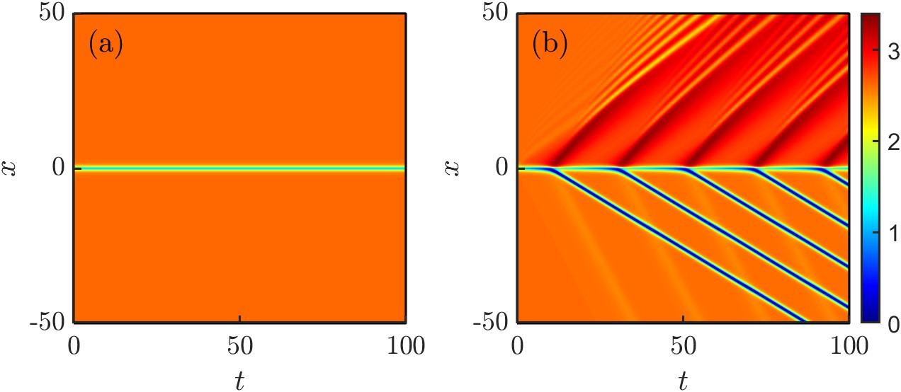
Figure 1: Dynamics ensuing from a 1D defect running through the BEC for $\mu=1$ and $\lambda=0.75$. (a) Subcritical case corresponding to a velocity $c=0.647$ below the speed of sound. The resulting steady state is stable. (b) Supercritical case corresponding to a velocity $c=0.7$ above the speed of sound. The resulting dynamics cannot feature a stationary state and, consequently, gives rise to a periodic emission of dark solitons in its wake.

For large enough $c$, namely past the speed-of-sound threshold, as it is the case for the pure cubic NLS nonlinearity without the LHY correction Hakim (1997); Carretero-González et al. (2007), the co-moving steady state can no longer be supported (it has terminated in a saddle-center bifurcation as we show below) and consequently emits a periodic train of dark solitons in its wake. Essentially, the emission of the solitary waves renders the dynamics temporarily and locally subcritical. Yet, once the solitary wave has moved enough upstream, the defect region becomes supercritical anew and yields an additional dark solitary structure, eventually resulting in the production of a train thereof. A example of this behavior is depicted in Fig. 1. The left panel shows how a defect running at low enough velocities gives rise to a stable co-moving steady state. However, past a critical value of the speed, as shown in the right panel, this steady state disappears through a bifurcation as illustrated below, resulting in the production of a periodic train of dark solitons. As the speed of the defect is increased further the spacing between the dark soliton emissions decreases.

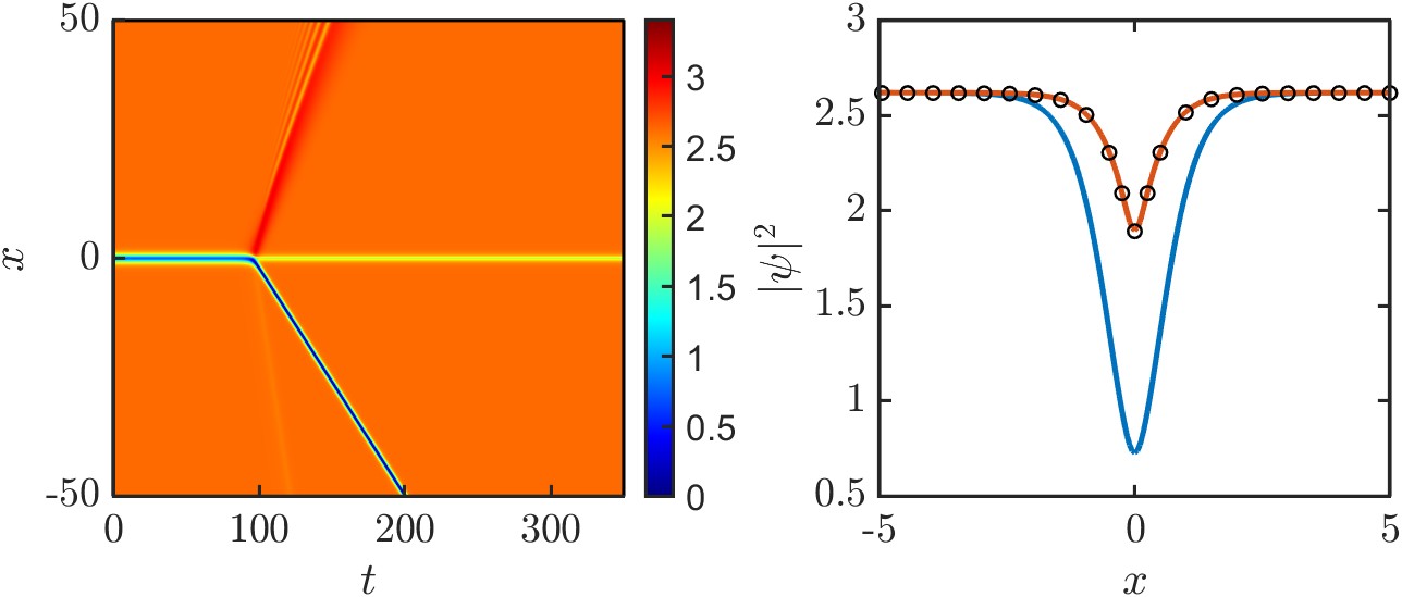
Figure 2: Evolution of the 1D unstable solution for a defect velocity $c=0.7$ below the speed of sound for $\mu=1$ and $\lambda=0.4$. The left panel shows the evolution where the deeper unstable steady state solution sheds a single dark soliton and settles to an apparently stable shallower solution. The right panel confirms that the initial unstable steady state (blue curve) decays (after the emission of the single dark soliton) to a shallower solution (red curve) that precisely corresponds to the stable steady state solution for this speed (circles).

Figure 3: (Color online) Top: Bifurcation diagram for the stable (lower part of the corresponding branches) and unstable (upper part of the branches) branches in 1D as the velocity of the impurity $c$ is varied for $\mu=1$ and for three values of the impurity strength $\lambda$ as indicated in the legend. The effective mass of the solution (see text) is plotted vs. $c$. As $c$ reaches a threshold value, the upper and lower branches coalesce in a saddle-center bifurcation (see point H). For values of $c$ larger than this threshold, there no longer exists a stable stationary state and hence the time evolution dynamics periodically sheds dark solitons in its wake (see right panel in Fig. 1). The vertical black line corresponds to the theoretical prediction of speed of sound in Eq. (10). Middle (bottom): Corresponding density (phase) profiles at the different values of $c$ indicated by the black dots in the top panel. Each subpanel depicts the corresponding unstable (deep; see blue curve) and stable (shallow; see red curve) solutions.

In order to numerically determine the critical speed for dark soliton emission, we study the steady states that exist as the defect velocity is varied. In particular, as it is the case for the pure NLS case without the LHY correction (see for instance Ref. Hakim (1997)), for values of $c$ below the speed-of-sound threshold, there exist two steady state solutions: a relatively shallow stable state and a relatively deep unstable steady state. For example, Fig. 2 depicts the evolution of the unstable solution for $c$ below the speed of sound. This deeper solution decays, after the emission of a single dark soliton, to a shallower solution that precisely corresponds to the stable solution. We can now trace the families of unstable (deeper) and stable (shallower) solutions as the parameters of the system are varied. In particular, in Fig. 3 we follow using pseudo-arclength continuation in $c$ these solution branches for several values of the defect strength $\lambda$. To monitor the solutions, we use the effective mass of the solution:

$$M_{\rm eff}=\int_{-\infty}^{+\infty}\left[|\alpha|^{2}-|\psi|^{2}\right]\,dx,$$ (17)

where $|\alpha|$ is the background level as defined in Eq. (5). According to this definition, the deeper the solution the higher the effective mass.

Figure 4: Critical values of defect strength $\lambda$ vs. defect speed $c$ for the 1D case. For each value of $c$ we extract the value of $\lambda$ where the saddle-center bifurcation occurs (collision between the deep and shallow steady state solutions). The vertical dashed line corresponds to the theoretical prediction of the speed of sound in Eq. (5). The inset shows a zoomed-in version for small defect strengths.

As can be seen in Fig. 3, the deep and shallow solutions, corresponding respectively to the upper and lower solution branches, coalesce (see the turning point H) as the defect velocity $c$ is increased. At a critical value of $c$, a saddle-center bifurcation ensues where the two solutions collide. Past this critical value of $c$, the system bears no stable solution and, hence, as explained above, periodic emission of dark solitons takes place at the wake of the impurity as seen in the right panel in Fig. 1. In Fig. 3 we also depict the theoretical prediction for the speed of sound of Eq. (10) (see vertical black line). As seen in Fig. 3, the defects always have a critical speed that is below the speed of sound. This suggests that defects will emit dark soliton trains for values slightly below the speed of sound. Nonetheless, the figure also suggests that the critical speed value tends to approach the speed of sound as the defect strength $\lambda$ decreases. In fact, as the computation of the speed of sound in Sec. II relies on small perturbations, the results will be valid in the limit of $\lambda\rightarrow 0$. To elucidate this connection, we depict in Fig. 4 the values of the defect strength $\lambda$ where the saddle-center collision between the deep and shallow steady state occurs. As it can be corroborated (see inset), the critical velocity tends to coincide with the theoretical speed of sounds $c_{s}$ of Eq. (5) when the defect strength $\lambda$ tends to zero.

III.2 Two-dimensional setting

We now proceed in a similar way as for the 1D case of the previous section but now for the 2D model of Eq. (11). Here we choose a 2D defect in the form of a ‘bar’ that is thin in the direction of the defect movement (namely the $x$-direction) and relatively wide in the transverse direction. Specifically, the 2D defect is taken to be

$$V_{\rm 2D}(x,y)=V_{\rm 1D}(x)\,\exp\left(\frac{-y^{2}}{2\epsilon_{y}^{2}}\right).$$

Note that we do not use the typical normalization constant for a 2D Gaussian as we are considering the thin defect $x$-direction the one that drives the nucleation of dark solitons and thus, to best compare with the 1D results, we use the same normalization prefactor as for the 1D case. For our numerical results below, we choose a thin defect bar with $\epsilon_{x}=1/\sqrt{2}\approx 0.707$ and a relatively wide lateral extent with $\epsilon_{y}=5$.

Figure 5: (Color online) Evolution corresponding to a supercritical 2D defect running at velocity $c=0.8$ for $\mu=0.5$ and $\lambda=0.92$. The defect impurity periodically emits a vortex-anti-vortex pair in its wake (only two pairs shown here for $t\leq 55$). (a) $t=0$, (b) $t=20$, (c) $t=35$, and (d) $t=55$.

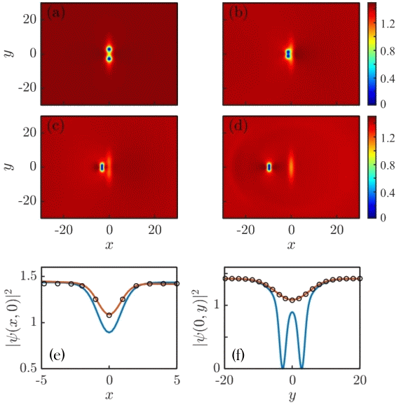
Figure 6: Evolution of the 2D unstable solution for a defect velocity $c=0.2$ below the speed of sound for $\mu=0.5$ and $\lambda=0.92$. Panels (a)–(d) show the evolution where the deeper unstable steady state solution sheds a vortex-anti-vortex pair and settles to the stable shallower solution. (a) $t=0$, (b) $t=55$, (c) $t=60$, and (d) $t=75$. Panel (e) and (f) depict the $y=0$ and $x=0$ cuts of the density confirming that the initial unstable steady state (blue curves) decay (after the emission of the vortex pair) to a shallower solution (red curves) that precisely corresponds to the stable steady state solution (shown by circles).

As in 1D, for sufficiently large, supercritical, velocities, the 2D defect will not support a stable stationary state and will, accordingly, emit a periodic train in its wake. In the 2D case, the defect produces a train of vortex-anti-vortex pairs. A typical example depicting multiple vortex shedding instances is shown in Fig. 5 (larger times produce more vortex-anti-vortex shedding; results not shown here). Also, as in the 1D case, the 2D model also features two steady state solutions for subcritical defect speeds: an unstable relatively deep one and a stable relatively shallow one. Figure 6 confirms, similar to what we saw for the 1D case, that for subcritical velocities, the deeper solution is unstable and, as it destabilizes, it sheds a single vortex-anti-vortex pair and eventually settles to the shallower stable steady state.

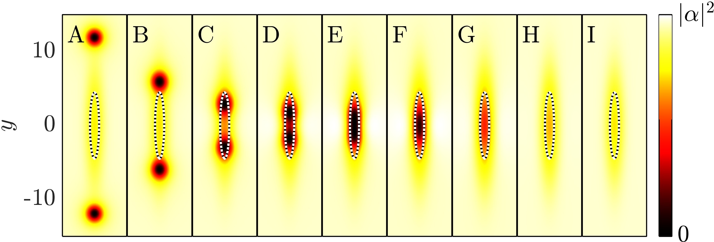
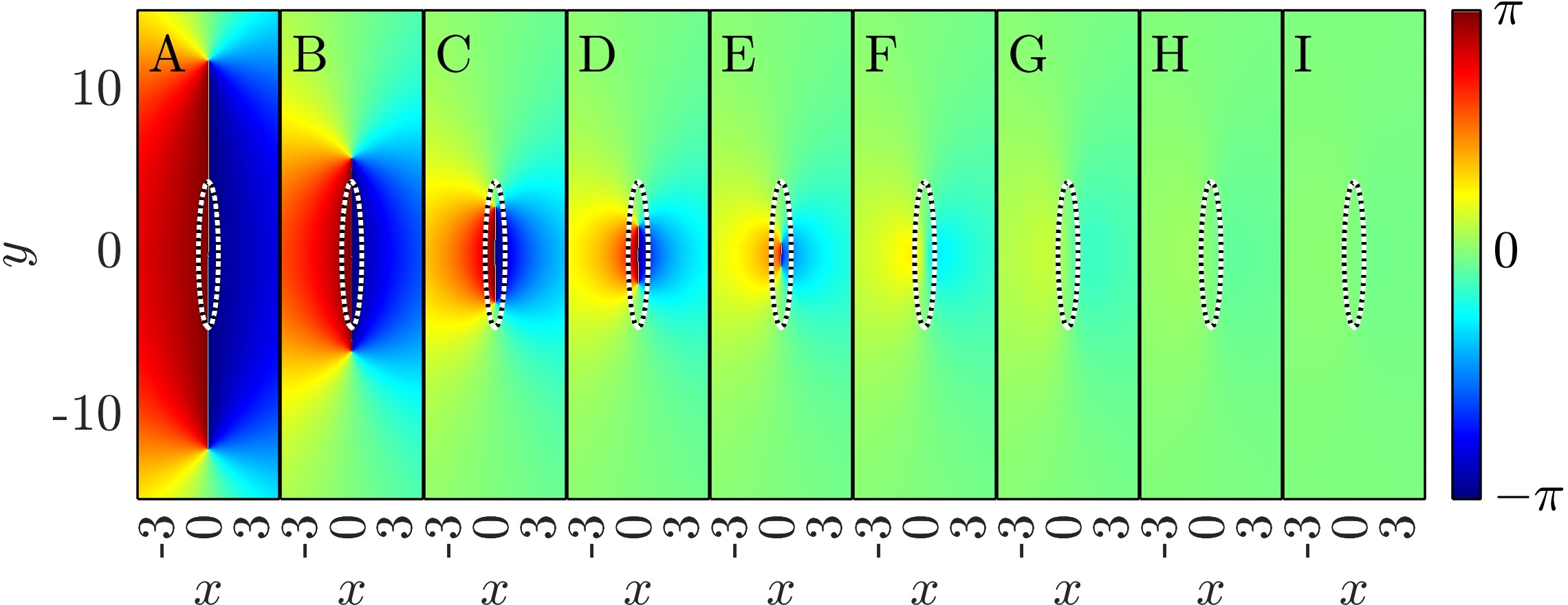
Figure 7: (Color online) Top: Similar to Fig. 3 but for the 2D case for $\mu=0.5$. The vertical black line corresponds to the theoretical prediction of speed of sound in Eq. (13). Middle (bottom): Corresponding density (phase) profiles at the different values of $c$ indicated by the black dots in the top panel. The dashed curve represents the isocontour level of the potential $V_{\rm 2D}$ at 2/3 of its maximum height.

By monitoring the effective mass as in Eq. (17), but replacing the single $x$-integral by an integral over the whole 2D domain and adjusting the background as per Eq. (12), we follow, using pseudo-arclength continuation, the bifurcation diagram of subcritical 2D solutions. The resulting bifurcation diagram for $\mu=0.5$ and for three different values of $\lambda$ is depicted in Fig. 7. Interestingly, in this 2D case, the upper branch of steady state solutions contains, for small enough values of the defect speed (namely $c<0.52$), a vortex-anti-vortex pair (see panels A–E). This is precisely the vortical structure pair that detaches from this unstable solution as it is evolved in time and finally settles to the corresponding stable lower branch solution, which in turn lacks any vortices (see for instance the dynamical evolution depicted in Fig. 6). It is also noteworthy that for small values of the running speed $c$, the steady state vortex pair contains vortices that are relatively far away from the defect impurity (see for instance profile in panel A which corresponds to a velocity $c=0.025$). As $c$ increases, the vortices of the upper branch solution get closer to the defect impurity. Further increasing $c$ induces the vortices to get closer to each other within the impurity until they merge and disappear (in the present case of $\lambda=0.92$ at an approximate value of $c=0.52$). Continuing past this vortex-merging point along the branch, the upper and lower solutions bifurcate from each other (or, equivalently, terminate) in a saddle-center bifurcation (case G in Fig. 7).

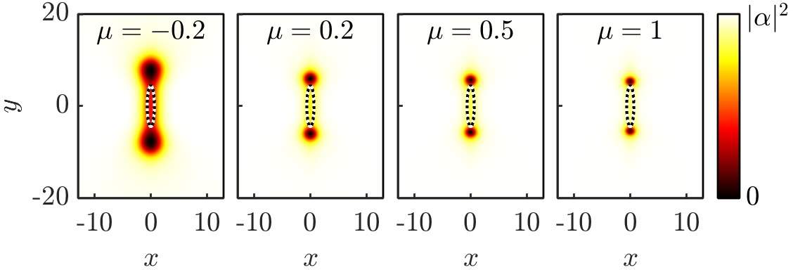
Figure 8: Density profile of unstable solutions in the 2D case for $\lambda=0.71$ and $c=0.1$ for the different values of $\mu$ as indicated in the panels. The dashed curve represents the isocontour level of the potential $V_{\rm 2D}$ at 2/3 of its maximum height.

The astute reader may have noticed the oscillatory behavior of the effective mass for the upper branch solutions for small values of $c$ in Fig. 7. This oscillatory behavior is missing in the 1D case (see bifurcation curves in Fig. 3). We attribute these oscillations to the existence of the vortex pairs attached to the corresponding steady states. As the vortices move closer to the impurity and run through it when $c$ is varied, they affect the effective mass and, thus produce, these small oscillations. In Fig. 8 we show the effects of varying the chemical potential $\mu$ on the upper branch steady state containing a pair of vortices attached at the end of the defect impurity. The existence of vortices for a wide range of $\mu$ values suggests that the above-mentioned oscillations of the effective mass will be visible for other values of the chemical potential. Additionally, the phenomenology discussed herein is present for different values of $\mu$. However, the main feature that chiefly appears to change is the size of the vortices which shrinks, as the healing length shrinks for increasing $\mu$. Moreover, for $\mu<0$, we can observe an implication of the droplet nature of the configuration and the effective surface tension in such a setting, namely a density modulation of the structure between the vortices, a feature far less noticeable in the cases of larger $\mu$.

Figure 9: Critical values of defect strength $\lambda$ vs. defect speed $c$ for the 2D case. Same layout as in Fig. 4. The vertical dashed line corresponds to the theoretical prediction of the speed of sound in Eq. (12), which is tantamount to the limit of $\lambda\rightarrow 0$. The inset shows a zoomed-in version for small defect strengths.

Finally, let us now compare the theoretical estimation of the speed of sound as per Eq. (13) and the critical value of the velocity in 2D. For this purpose, we depict in Fig. 9 the values of the defect strength $\lambda$ where the saddle-center collision between the deep and shallow steady states occurs. As the inset corroborates, the critical velocity coincides reasonably well with the theoretical speed of sounds $c_{s}$ when the defect strength $\lambda$ tends to zero, with the difference being attributable to the approximations within the numerical computations.

III.3 Three-dimensional setting

Let us now study the 3D model of Eq. (14). In this case we chose a defect impurity with the shape of a rectangular plate that is thin in the direction of the defect movement (namely the $x$-direction) and relatively wide in the other two transverse directions. Specifically, we use the 3D defect

$$V_{\rm 3D}(x,y,z)=V_{\rm 1D}(x)\,H_{w_{z}}(z)\,H_{w_{y}}(y)$$

with $\epsilon_{x}=1/4$, $w_{y}=8$ and $w_{z}=4$ and where $H_{w}$ is a smoothed 1D top-hat function given by

$$H_{w}(r)=\frac{1}{4}\left[\tanh\left(\frac{w}{2}+r\right)+1\right]\left[\tanh\left(\frac{w}{2}-r\right)+1\right].$$

As it was the case for 1D and 2D setting above, we take a relatively thin Gaussian profile along the direction of motion. In the transverse directions we take a relatively large (when compared to the thin longitudinal direction) rectangular plate. One of the motivations to use a rectangular plate is to observe the effects of this anisotropy in the transverse directions. Naturally, an isotropic, namely circular, defect plate would give rise to a perfectly isotropic steady state solution, which in turn, when supersonic, would nucleate a symmetric vortex ring (results not shown here).

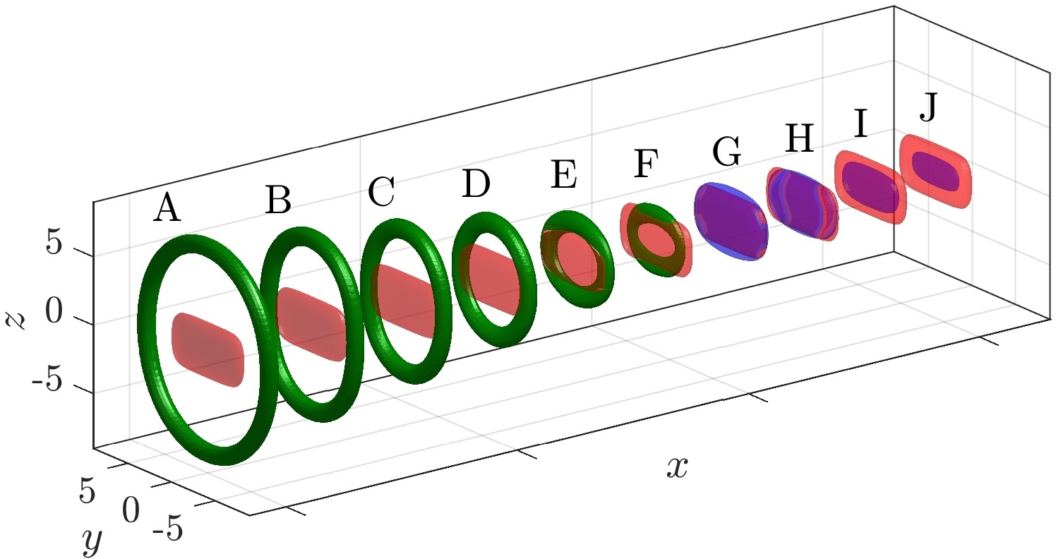
Figure 10: (Color online) Top: Bifurcation diagram for the stable and unstable branches in 3D for $g_{1}=1$ and $\mu=0.5$ and for the values of $\lambda$ indicated in the legend. Similar layout and meaning as in Fig. 3. The vertical black line corresponds to the theoretical prediction of the 3D speed of sound in Eq. (16). Bottom: Corresponding profiles at the different values of $c$ indicated by the black dots in the top panel. Each instance depicts an isocontour of the corresponding vorticity (solid green) together with an isocontour of the 3D defect potential $V_{\rm 3D}$ at 1/2 of its maximum amplitude (transparent red). The points corresponding to G–J do not carry a sizeable amount of vorticity and thus isocontours of the density are shown instead (transparent blue).

Similarly to what we observe in the 1D and 2D cases, the 3D model also gives rise to two branches of subcritical steady state solutions. These two solution branches correspond to unstable, relatively large (when compared to the size of the defect), vortex rings and stable density depletions. We monitor the effective mass as in Eq. (17), but replacing the single $x$-integral by an integral over the whole 3D domain and adjusting the background as per Eq. (15). As before, we use pseudo-arclength continuation to follow these branches of subcritical 3D steady state solutions. The results for $g_{1}=1$ and $\mu=0.5$ are depicted in Fig. 10 for three different values of the defect strength $\lambda$. It is interesting to notice that in the limit of small defect speed $c$, the upper branch of unstable solutions corresponds to large vortex rings that are larger than, and seemingly detached from, the impurity. On the other hand, the stable steady states, corresponding to density depletions that do not carry vorticity, are tightly attached to the defect. This provides a physical explanation for their corresponding stability as the larger ring, being further away from the defect, detaches through the instability. On the other hand the smaller density depletion is tightly attached to the impurity and is found to be dynamically stable. Another interesting feature is that for intermediate values of the velocity, the vortex ring has the opposite aspect ratio than that of the defect plate. See for instance the vortex ring corresponding to the points B and C which are taller than wider while the defect is, oppositely, wider than taller. Therefore, the effect of the anisotropy of the defect plate is to typically create vortex rings that lack circular symmetry and that are slightly “squeezed” in the horizontal or vertical direction. This is to be contrasted with the case of a circular plate that would nucleate a perfectly symmetric, circular, steady state and, in turn, shed a symmetric vortex ring (results not shown here). The asymmetry present in the unstable steady state is inherited by the vortex rings that are nucleated from the unstable subcritical steady state as well as the train of vortex rings that are nucleated from the defect impurity running at supercritical speeds. This asymmetry means that the vortex rings nucleated by the defect will contain Kelvin (vibrational) modes Simula et al. (2008); Chevy and Stringari (2003) that will induce internal oscillations (see Fig. 11).

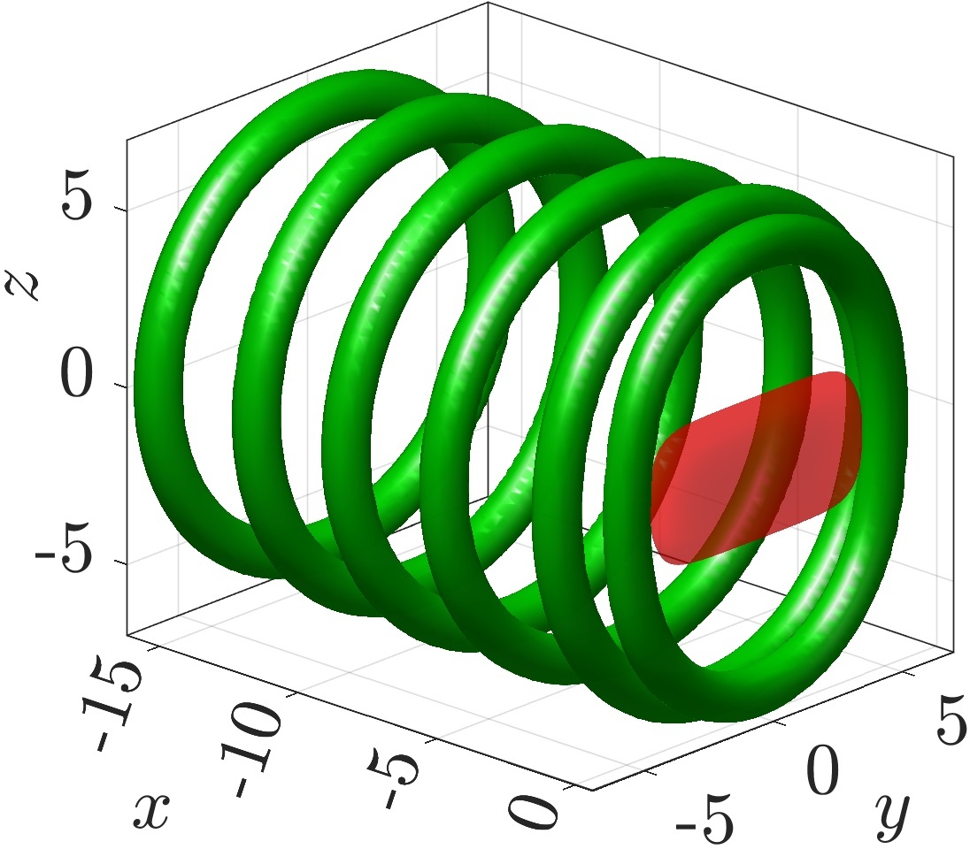
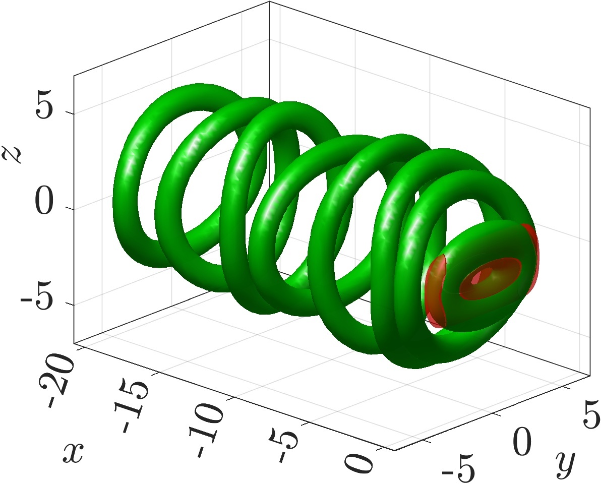
Figure 11: (Color online) Examples of vortex ring emission from the unstable steady state solution. Each panel depicts overlaid snapshots of the vorticity (green surfaces) at different times during the emission of a single vortex ring from the defect (shown in red) on a co-moving reference frame. The left and right panel corresponds, respectively, to the ensuing dynamics from cases B and F in Fig. 10. Namely, for $\lambda=1.3$, $\mu=0.5$, $g_{1}=1$, and $c=0.3224$ (case B; left panel) and $c=0.5124$ (case F; right panel). The times for the snapshots for cases B and F are, respectively, $t=\{0,160,220,280,340,400\}$ and $t=\{0,90,100,120,140,160,180,200\}$, from the closest vortex ring to the defect to the one furthest away.

Let us now follow in more detail the nucleation of vortex rings from the unstable branch of solutions. In particular, we depict in Fig. 11 the evolution of the unstable steady states corresponding to cases B (left panel) and F (right panel) of Fig. 10. The simulations depict how the vortex ring, that is pinned by the defect, detaches (by virtue of the solution’s instability) and then travels downstream. It is worth reminding that, as per our setup in Sec. II, we are always mounted in a co-moving reference frame on top of the running defect. As mentioned above, the pinned vortex rings are asymmetric as per our choice of defect that has a rectangular transverse (i.e., perpendicular to its motion) cross section. Therefore, the detaching vortex rings are not circular and thus are prone to Kelvin, internal, oscillatory modes. It is also interesting to note that the larger vortex rings, corresponding to relatively small values of the running defect speed $c$, detach and keep their relatively large radius —cf. case B corresponding to the left panel in Fig. 11. On the other hand, for larger defect speeds, the pinned vortex ring has a small radius and thus expands as it detaches —cf. case F corresponding to the right panel in Fig. 11. It is also worth mentioning that the detached vortex rings do not travel downstream at velocity $c$ with the background fluid velocity. This is because the detached vortices (and also the nucleated vortices for supercritical speeds) have an intrinsic velocity $v_{i}$ that goes against the background flow (see Ref. Caplan et al. (2014) and references therein). Thus, vortex rings do travel downstream but with a slower velocity than the background flow corresponding to $c-v_{i}$.

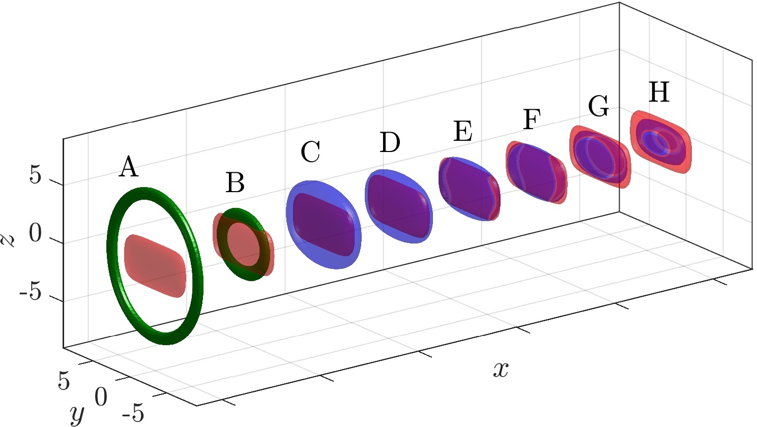
Figure 12: (Color online) Same as in Fig. 10 but for constant $\lambda=1.3$ and $g_{1}=-1$ for the values of $\mu$ indicated in the legend. In this case, the points corresponding to C–H do not carry a sizeable amount of vorticity and thus density isocontours are shown instead.

Finally, since it may be physically relevant to consider negative values of $g_{1}$ in the 3D model (14), we depict in Fig. 12 the bifurcation diagram for the steady state solutions for $g_{1}=-1$ and a defect strength of $\lambda=1.3$ for three different values of the chemical potential $\mu$. The results are similar as the ones presented for $g_{1}=1$ in Fig. 10 with no significant qualitative differences.

IV Conclusions & Future Challenges

We have studied the effects of running an impurity defect through a Bose-Einstein condensate in a regime that takes into account the incorporation of the Lee-Huang-Yang (LHY) correction that gives rise to quantum droplets. We systematically explored the 1D, 2D, and 3D cases that feature different nonlinear LHY corrections. For all dimensionalities, we followed, using pseudo-arclength continuation, the two subcritical solution branches that exist for defect velocities below the critical speed and which feature a localized waveform co-traveling with the defect. These solutions correspond to dark solitons, vortex-anti-vortex pairs, and vortex rings for, respectively, the 1D, 2D, and 3D cases. In all cases we find that there exist an upper and lower branch of solutions connected through a saddle-center bifurcation. The upper branch is found to always be unstable and corresponds to a solution that has a relatively larger effective mass and a nonlinear state further detached from the defect. In contrast, the lower solution branch of relatively smaller effective mass is dynamically stable for subcritical velocities and features a state more closely bound to the defect. When dynamically evolved, the solution on the upper branch always destabilizes by shedding a single coherent structure and then settling to its lower branch, stable, sibling solution. By using a perturbation approach we are able to theoretically predict the corresponding speed of sound of the medium which, in turn, takes a different functional form for the different model dimensionalities. We corroborate that the theoretically computed speed of sounds does match the bifurcation point (where the upper and lower branches collide) as the strength of the defect tends to zero and we identify how this critical speed (and the corresponding saddle-center bifurcation point) deviates, i.e., decreases from this threshold, as we move into the finite defect strength case. In the 3D case we showcase the effect of using an anisotropic defect in the transverse direction. This anisotropy is responsible for the formation of “squeezed” vortex rings again featuring a similar bifurcation diagram. We explored the relevant phenomenologies not only as a function of the dragging speed and the defect strength, but also in terms of the chemical potential variations, observing the variation of the states as the droplet (negative chemical potential) limit is approached. Finally, we also performed dynamics in the supercritical case, observing how the disappearance of the states co-traveling with the defect results in the emission of a train of dark solitons, or a street of vortices or an array of vortex rings in 1D, 2D and 3D, respectively.

The present work naturally suggests numerous additional considerations in the context of nonlinear wave patterns embedded in the types of droplet models that were considered herein. While some studies along this vein have recently taken place both in 1D Kartashov et al. (2022); edmonds and in higher dimensions Luo et al. (2021), it appears that a detailed understanding of dark solitons, vortices or vortex pairs and vortex rings embedded within droplet configurations is largely still missing, as is a characterization of their stability and dynamics. We believe that such a systematic study and also comparison with beyond mean-field models (see for a recent review Ref. Mistakidis et al. (2022)) would be of particular interest in future work. Such topics are presently under consideration and will be reported in future publications.

Appendix A Speed of sound in 2D

Looking for solutions to Eq. (11) of the form of Eq. (6) but in 2D yields

$$cR_{x} = \frac{1}{2}(2R_{x}\phi_{x}+R\phi_{xx}+2R_{y}\phi_{y}+R\phi_{yy}),$$ (18)

$$cR\phi_{x} = -\frac{1}{2}(R_{xx}+R_{yy}-R\phi_{x}^{2}-R\phi_{y}^{2})$$ (19)

$$+R^{3}\ln{R^{2}}-\mu R+VR.$$

Further linearizing and expanding the phase and density terms by using transverse modes of wavenumber $k$ in the $y$-direction as $\phi(x,y,t)=\epsilon\,\theta(x,t)e^{iky}$ and $R(x,y,t)=|\alpha|+\epsilon\,r(x,t)e^{iky}$, Eqs. (18) and (19) become

$${2cr_{x}} = |\alpha|\left(\theta_{xx}-k^{2}\theta\right),$$ (20)

$$r_{xx} = -2c|\alpha|\theta_{x}+r(k^{2}+4|\alpha|^{2}+4\mu),$$ (21)

Finally, by making the substitutions $r=ae^{\Lambda x}$ and $\theta=be^{\Lambda x}$, Eqs. (18) and (19) read

$$A\begin{bmatrix}a\\ b\end{bmatrix}=\begin{bmatrix}0\\ 0\end{bmatrix},$$

where

$$A=\begin{bmatrix}{2c\Lambda}/{|\alpha|}&~{}~{}k^{2}-\Lambda^{2}\\[8.61108pt] k^{2}+4|\alpha|^{2}+4\mu-\Lambda^{2}&~{}~{}-2|\alpha|\Lambda.\end{bmatrix}$$

Then, setting $\det(A)=0$ with $k=0$ and $\Lambda=0$ yields the speed of sound for the 2D setting as

$$c_{s}=\sqrt{|\alpha|^{2}+\mu}.$$ (22)

We test this prediction numerically under different settings in Sec. III.2.

Appendix B Speed of sound in 3D

Looking for solutions to Eq. (11) of the form of Eq. (6) but now in 3D yields

$$2cR_{x} = 2R_{x}\phi_{x}+R\phi_{xx}+2R_{y}\phi_{y}+R\phi_{yy}$$ (23)

$$+2R_{z}\phi_{z}+R\phi_{zz}$$

$$cR\phi_{x} = -\frac{1}{2}(R_{xx}-R\phi_{x}^{2}+R_{yy}-R\phi_{y}^{2}+R_{zz}-R\phi_{z}^{2})$$ (24)

$$+R^{4}+g_{1}R^{3}-\mu R+VR$$

As in the 2D calculations, we now allow for the density and phase terms to contain transverse modes. In this case, including modes in the $y$ and $z$ directions as $\phi(x,y,z,t)=\epsilon\,\theta(x,t)e^{ik_{y}y}e^{ik_{z}z}$ and $R(x,y,t)=|\alpha|+\epsilon\,r(x,t)e^{ik_{y}y}e^{ik_{z}z}$. Then, after linearization, Eqs. (23) and (24) become

$${2cr_{x}} = {|\alpha|}\left[\theta_{xx}-(k_{y}^{2}+k_{z}^{2})\theta\right],$$ (25)

$$r_{xx} = r\left[2|\alpha|^{3}+4\mu+(k_{y}^{2}+k_{z}^{2})\right]-2c|\alpha|\theta_{x}.$$ (26)

Using the substitutions $r=ae^{\Lambda x}$ and $\theta=be^{\Lambda x}$ yields the linear system

$$A\begin{bmatrix}a\\ b\end{bmatrix}=\begin{bmatrix}0\\ 0\end{bmatrix},$$

where

$$A=\begin{bmatrix}{2c\Lambda}/{|\alpha|}&~{}~{}(k_{y}^{2}+k_{z}^{2})-\Lambda^{2}\\[8.61108pt] (k_{y}^{2}+k_{z}^{2})+2|\alpha|^{3}+4\mu-\Lambda^{2}&~{}~{}-2c|\alpha|\Lambda\end{bmatrix}$$

Finally, setting $\det(A)=0$ and $k_{y}=k_{z}=0$ and $\Lambda=0$ yields the expression for the speed of sound in the 3D setting

$$c_{s}=\sqrt{\frac{|\alpha|^{3}+2\mu}{2}}.$$ (27)

Appendix C Speed of sound for the NLS

For comparison with the LHY case and for completeness, the next two sections show the results of the pure NLS model case:

$$i\partial_{t}A-ic\,\partial_{x}A=-\frac{1}{2}\nabla^{2}A+|A|^{2}A-\mu A+V\,A,$$ (28)

with $\nabla^{2}$ being the Laplacian and $V$ the corresponding defect potential. In contrast with the case with the LHY correction, the pure NLS model admits a single homogeneous steady state of density $|\alpha|^{2}=\mu$.

C.1 NLS case in 1D

Analyzing this case in a way similar to the one in Sec. II.1, indeed following the work of Ref. Hakim (1997), after replacing $A(x)=R(x)e^{i\phi(x)}$, the system

$$\phi_{x}R^{2} = \frac{1}{2}cR^{2}+C_{I},$$ (29)

$$cR\phi_{x} = -(R_{xx}-R\phi_{x}^{2})+R^{3}-\mu R+VR,$$ (30)

with the constant of integration $C_{I}=-\frac{1}{2}c\mu$. Solving for $\phi_{x}$ in Eq. (29) and replacing in it in Eq. (30) yields

$$R_{xx}=\frac{1}{4}c^{2}\left(-R+\frac{\mu^{2}}{R^{3}}\right)+R^{3}-\mu R+VR.$$

Linearizing as before, using $R(x)=|\alpha|+r(x)$, yields the following expression for the evolution of the perturbation:

$$r_{xx}=r(2\mu-c^{2}),$$

and, therefore, the speed of sound in 1D for the pure NLS case is given by

$$c_{s}=\sqrt{2\mu}.$$ (31)

The relevant calculation both in this section and in the next one is provided for reasons of completeness.

Figure 13: (Color online) Same as in Fig. 3 but for the standard (cubic) NLS model (28) in 1D without the LHY correction. The value of $\mu=|\alpha|^{2}$ was chosen here so as to match the background density supporting the dark solitons for the LHY case. In this case, the theoretical prediction for the speed of sound is given by Eq. (31). Note the similarity with the results of the LHY case in Fig. 3, albeit with a different scale in the $c$-axis.

In Fig. 13 depicts the numerical results corresponding to the standard 1D NLS model (28). These results are to be compared with the corresponding ones in Fig. 3 that include the LHY correction as per Eq. (4). When comparing the two cases at first glance, little difference is observed. However, do note the quite different scales of defect speeds $c$ such that the velocities for the standard NLS case are about twice of those with the LHY correction.

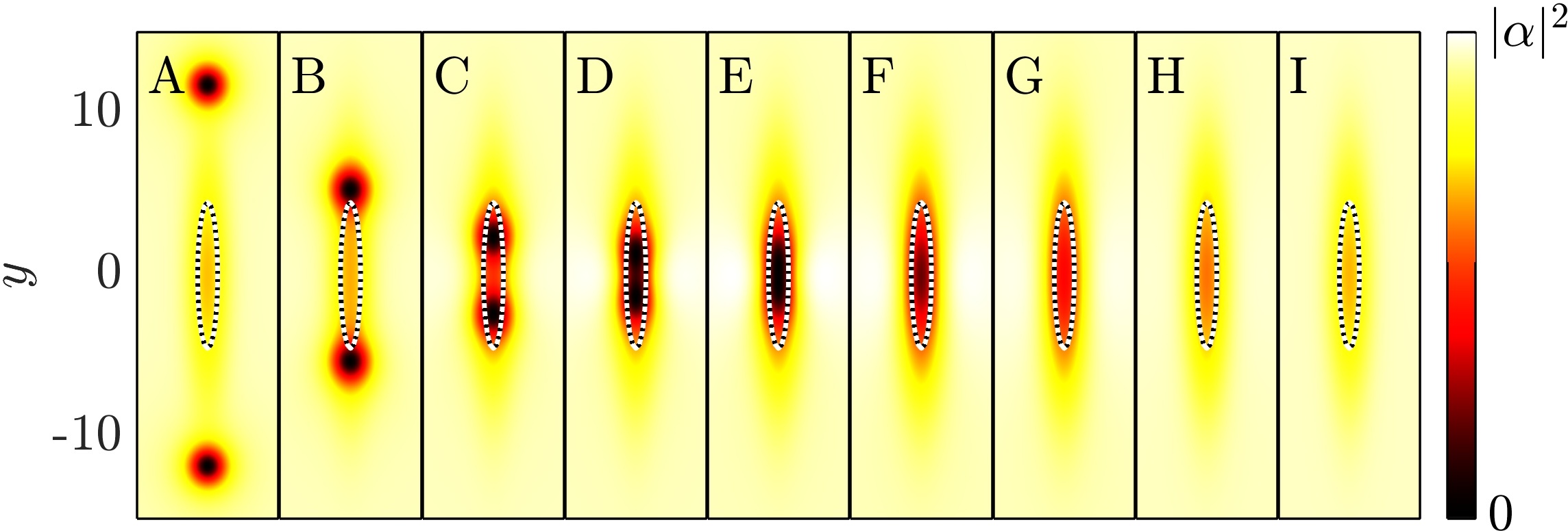
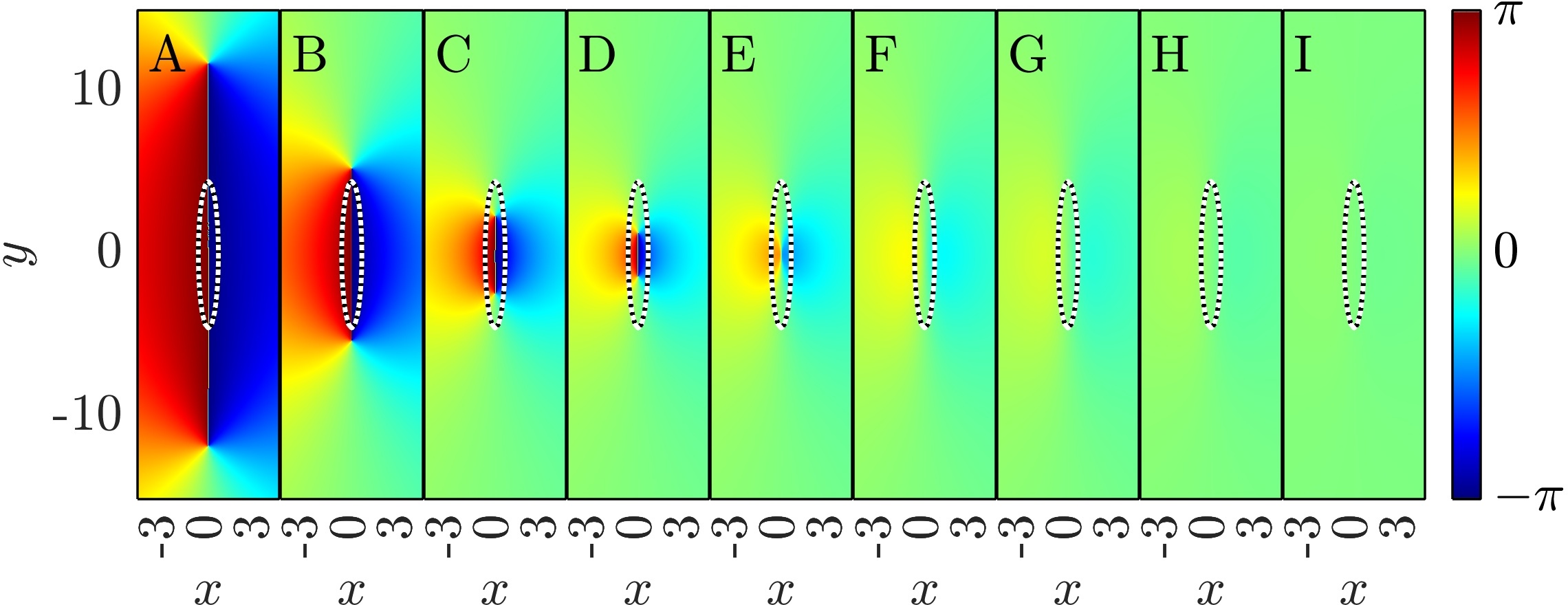
Figure 14: (Color online) Similar to Fig. 7 but for the standard NLS 2D model without the LHY correction. The vertical line in the top panel is the predicted speed of sound for the pure NLS in 2D given by Eq. (34).

C.2 NLS case in 2D

Following a very similar analysis to the one in Sec. II.2 and Appendix A yields, after (i) separating density and phase by $A(x,y,t)=R(x,y,t)e^{i\phi(x,y,t)}$, (ii) expanding in transversal modes by using $\phi(x,y,t)=\epsilon\theta(x,t)e^{iky}a$, (iii) linearizing the perturbed solution using $R(x,y,t)=r_{0}+\epsilon r(x,t)e^{iky}$, and (iv) some algebra, yields, to first order the system:

$$\frac{2cr_{x}}{r_{0}} = \theta_{xx}-k^{2}\theta,$$ (32)

$$r_{xx} = -2cr_{0}\theta_{x}+r(k^{2}+4\mu).$$ (33)

Then, making the substitutions $r=ae^{\lambda x}$ and $\theta=be^{\lambda x}$, yields the matrix system which induces the following matrix system

$$\begin{bmatrix}\frac{2c\lambda}{r_{0}}&k^{2}-\lambda^{2}\\[4.30554pt] k^{2}+4\mu-\lambda^{2}\quad&-2cr_{0}\lambda\end{bmatrix}\begin{bmatrix}a\\[4.30554pt] b\end{bmatrix}=\begin{bmatrix}0\\[4.30554pt] 0\end{bmatrix}.$$

Setting the determinant equal to zero then yields the characteristic polynomial

$$-\lambda^{4}+\lambda^{2}(-4c^{2}+2k^{2}+4\mu)-k^{2}(k^{2}+4\mu)=0,$$

which implies that, for the most unstable mode $k=0$, the speed of sound for the standard NLS model in 2D is given by

$$c_{s}=\sqrt{\mu}.$$ (34)

Figure 14 depicts the numerical results corresponding to the standard 2D NLS model (28). These results are very similar to the corresponding ones in Fig. 7 that include the LHY correction as per Eq. (11). As it was the case for the droplet model, the NLS also displays a non-monotonic behavior of the effective mass as $c$ decreases for the upper branch. We again attribute this behavior to the appearance of the vortices that start, for small $c$, far away from the impurity and then get closer to it as $c$ increases (see middle set of panels in Fig. 14).

References

- Pethick and Smith (2008) C. J. Pethick and H. Smith, Bose-Einstein condensation in dilute gases (Cambridge university press, 2008).
- Stringari and Pitaevskii (2003) S. Stringari and L. Pitaevskii, Bose-Einstein Condensation (Oxford University Press, Oxford, United Kingdom, 2003).
- Kevrekidis et al. (2015) P. G. Kevrekidis, D. J. Frantzeskakis, and R. Carretero-González, The defocusing nonlinear Schrödinger equation: from dark solitons to vortices and vortex rings (Society for Industrial and Applied Mathematics, Philadelphia, PA, 2015).
- Raman et al. (1999) C. Raman, M. Köhl, R. Onofrio, D. S. Durfee, C. E. Kuklewicz, Z. Hadzibabic, and W. Ketterle, “Evidence for a critical velocity in a Bose-Einstein condensed gas,” Phys. Rev. Lett. 83, 2502 (1999).
- Onofrio et al. (2000) R. Onofrio, C. Raman, J. M. Vogels, J. R. Abo-Shaeer, A. P. Chikkatur, and W. Ketterle, “Observation of superfluid flow in a Bose-Einstein condensed gas,” Phys. Rev. Lett. 85, 2228 (2000).
- Engels and Atherton (2007) P. Engels and C. Atherton, “Stationary and nonstationary fluid flow of a Bose-Einstein condensate through a penetrable barrier,” Phys. Rev. Lett. 99, 160405 (2007).
- Frisch et al. (1992) T. Frisch, Y. Pomeau, and S. Rica, “Transition to dissipation in a model of superflow,” Phys. Rev. Lett. 69, 1644 (1992).
- Winiecki et al. (1999) T. Winiecki, J. F. McCann, and C. S. Adams, “Pressure drag in linear and nonlinear quantum fluids,” Phys. Rev. Lett. 82, 5186 (1999).
- Hakim (1997) V. Hakim, “Nonlinear Schrödinger flow past an obstacle in one dimension,” Phys. Rev. E 55, 2835 (1997).
- Leboeuf and Pavloff (2001) P. Leboeuf and N. Pavloff, “Bose-Einstein beams: Coherent propagation through a guide,” Phys. Rev. A 64, 033602 (2001).
- Pavloff (2002) N. Pavloff, “Breakdown of superfluidity of an atom laser past an obstacle,” Phys. Rev. A 66, 013610 (2002).
- Brazhnyi and Kamchatnov (2003) V. A. Brazhnyi and A. M. Kamchatnov, “Creation and evolution of trains of dark solitons in a trapped one-dimensional Bose-Einstein condensate,” Phys. Rev. A 68, 043614 (2003).
- Hans et al. (2015) I. Hans, J. Stockhofe, and P. Schmelcher, “Generating, dragging, and releasing dark solitons in elongated Bose-Einstein condensates,” Phys. Rev. A 92, 013627 (2015).
- Radouani (2004) A. Radouani, “Soliton and phonon production by an oscillating obstacle in a quasi-one-dimensional trapped repulsive Bose-Einstein condensate,” Phys. Rev. A 70, 013602 (2004).
- Carretero-González et al. (2007) R. Carretero-González, P. Kevrekidis, D. Frantzeskakis, B. Malomed, S. Nandi, and A. Bishop, “Soliton trains and vortex streets as a form of cerenkov radiation in trapped Bose-Einstein condensates,” Mathematics and Computers in Simulation 74, 361 (2007), nonlinear Waves: Computation and Theory VI.
- Syafwan et al. (2016) M. Syafwan, P. Kevrekidis, A. Paris-Mandoki, I. Lesanovsky, P. Krüger, L. Hackermüller, and H. Susanto, “Superfluid flow past an obstacle in annular Bose-Einstein condensates,” Journal of Physics B: Atomic, Molecular and Optical Physics 49, 235301 (2016).
- Susanto et al. (2007) H. Susanto, P. G. Kevrekidis, R. Carretero-González, B. A. Malomed, D. J. Frantzeskakis, and A. R. Bishop, “Čerenkov-like radiation in a binary superfluid flow past an obstacle,” Phys. Rev. A 75, 055601 (2007).
- Rodrigues et al. (2009) A. S. Rodrigues, P. G. Kevrekidis, R. Carretero-González, D. J. Frantzeskakis, P. Schmelcher, T. J. Alexander, and Y. S. Kivshar, “Spinor Bose-Einstein condensate flow past an obstacle,” Phys. Rev. A 79, 043603 (2009).
- Larré et al. (2012) P.-E. Larré, N. Pavloff, and A. M. Kamchatnov, “Wave pattern induced by a localized obstacle in the flow of a one-dimensional polariton condensate,” Phys. Rev. B 86, 165304 (2012).
- Katsimiga et al. (2018) G. C. Katsimiga, S. I. Mistakidis, G. M. Koutentakis, P. G. Kevrekidis, and P. Schmelcher, “Many-body dissipative flow of a confined scalar Bose-Einstein condensate driven by a Gaussian impurity,” Phys. Rev. A 98, 013632 (2018).
- Petrov (2015) D. S. Petrov, “Quantum mechanical stabilization of a collapsing Bose-Bose mixture,” Phys. Rev. Lett. 115, 155302 (2015).
- Petrov and Astrakharchik (2016) D. S. Petrov and G. E. Astrakharchik, “Ultradilute low-dimensional liquids,” Phys. Rev. Lett. 117, 100401 (2016).
- Lee et al. (1957) T. D. Lee, K. Huang, and C. N. Yang, “Eigenvalues and eigenfunctions of a Bose system of hard spheres and its low-temperature properties,” Phys. Rev. 106, 1135 (1957).
- Cabrera et al. (2018) C. R. Cabrera, L. Tanzi, J. Sanz, B. Naylor, P. Thomas, P. Cheiney, and L. Tarruell, “Quantum liquid droplets in a mixture of Bose-Einstein condensates,” Science 359, 301 (2018).
- Cheiney et al. (2018) P. Cheiney, C. R. Cabrera, J. Sanz, B. Naylor, L. Tanzi, and L. Tarruell, “Bright soliton to quantum droplet transition in a mixture of Bose-Einstein condensates,” Phys. Rev. Lett. 120, 135301 (2018).
- Semeghini et al. (2018) G. Semeghini, G. Ferioli, L. Masi, C. Mazzinghi, L. Wolswijk, F. Minardi, M. Modugno, G. Modugno, M. Inguscio, and M. Fattori, “Self-bound quantum droplets of atomic mixtures in free space,” Phys. Rev. Lett. 120, 235301 (2018).
- Ferioli et al. (2019) G. Ferioli, G. Semeghini, L. Masi, G. Giusti, G. Modugno, M. Inguscio, A. Gallemí, A. Recati, and M. Fattori, “Collisions of self-bound quantum droplets,” Phys. Rev. Lett. 122, 090401 (2019).
- D’Errico et al. (2019) C. D’Errico, A. Burchianti, M. Prevedelli, L. Salasnich, F. Ancilotto, M. Modugno, F. Minardi, and C. Fort, “Observation of quantum droplets in a heteronuclear bosonic mixture,” Phys. Rev. Research 1, 033155 (2019).
- Chomaz et al. (2016) L. Chomaz, S. Baier, D. Petter, M. J. Mark, F. Wächtler, L. Santos, and F. Ferlaino, “Quantum-fluctuation-driven crossover from a dilute Bose-Einstein condensate to a macrodroplet in a dipolar quantum fluid,” Phys. Rev. X 6, 041039 (2016).
- Ferrier-Barbut et al. (2016) I. Ferrier-Barbut, H. Kadau, M. Schmitt, M. Wenzel, and T. Pfau, “Observation of quantum droplets in a strongly dipolar Bose gas,” Phys. Rev. Lett. 116, 215301 (2016).
- Li et al. (2018) Y. Li, Z. Chen, Z. Luo, C. Huang, H. Tan, W. Pang, and B. A. Malomed, “Two-dimensional vortex quantum droplets,” Phys. Rev. A 98, 063602 (2018).
- Zhang et al. (2019) X. Zhang, X. Xu, Y. Zheng, Z. Chen, B. Liu, C. Huang, B. A. Malomed, and Y. Li, “Semidiscrete quantum droplets and vortices,” Phys. Rev. Lett. 123, 133901 (2019).
- Morera et al. (2020) I. Morera, G. E. Astrakharchik, A. Polls, and B. Juliá-Díaz, “Quantum droplets of bosonic mixtures in a one-dimensional optical lattice,” Phys. Rev. Research 2, 022008 (2020).
- Mithun et al. (2020) T. Mithun, A. Maluckov, K. Kasamatsu, B. A. Malomed, and A. Khare, “Modulational instability, inter-component asymmetry, and formation of quantum droplets in one-dimensional binary Bose gases,” Symmetry 12, 174 (2020).
- Kartashov et al. (2018) Y. V. Kartashov, B. A. Malomed, L. Tarruell, and L. Torner, “Three-dimensional droplets of swirling superfluids,” Phys. Rev. A 98, 013612 (2018).
- Luo et al. (2021) Z. Luo, W. Pang, B. Liu, Y. Li, and B. A. Malomed, “A new form of liquid matter: quantum droplets,” Frontiers of Physics 16, 32201 (2021).
- Caplan and Carretero-González (2013) R. Caplan and R. Carretero-González, “Numerical stability of explicit Runge-Kutta finite-difference schemes for the nonlinear Schrödinger equation,” Appl. Numer. Math. 71, 24 (2013).
- Doedel (2007) E. J. Doedel, “Lecture notes on numerical analysis of nonlinear equations,” in Numerical Continuation Methods for Dynamical Systems: Path Following and Boundary Value Problems (Springer, 2007) pp. 1–49.
- Veltz (2020) R. Veltz, “BifurcationKit.jl,” (2020).
- Simula et al. (2008) T. Simula, T. Mizushima, and K. Machida, “Vortex waves in trapped Bose-Einstein condensates,” Phys. Rev. A 78, 053604 (2008).
- Chevy and Stringari (2003) F. Chevy and S. Stringari, “Kelvin modes of a fast rotating Bose-Einstein condensate,” Phys. Rev. A 68, 053601 (2003).
- Caplan et al. (2014) R. Caplan, T. J.D., R. Carretero-González, and K. P.G., “Scattering and leapfrogging of vortex rings in a superfluid,” Phys. Fluids 26, 097101 (2014).
- Kartashov et al. (2022) Y. V. Kartashov, V. M. Lashkin, M. Modugno, and L. Torner, “Spinor-induced instability of kinks, holes and quantum droplets,” New Journal of Physics 24, 073012 (2022).
- Mistakidis et al. (2022) S. I. Mistakidis, A. G. Volosniev, R. E. Barfknecht, T. Fogarty, T. Busch, A. Foerster, P. Schmelcher, and N. T. Zinner, “Cold atoms in low dimensions–a laboratory for quantum dynamics,” arXiv preprint arXiv:2202.11071 (2022), https://doi.org/10.48550/arXiv.2202.11071.