Affinity-VAE for disentanglement, clustering and classification of objects in multidimensional image data

Abstract

In this work we present affinity-VAE: a framework for automatic clustering and classification of objects in multidimensional image data based on their similarity. The method expands on the concept of $\beta$-VAEs with an informed similarity-based loss component driven by an affinity matrix. The affinity-VAE is able to create rotationally-invariant, morphologically homogeneous clusters in the latent representation, with improved cluster separation compared with a standard $\beta$-VAE. We explore the extent of latent disentanglement and continuity of the latent spaces on both 2D and 3D image data, including simulated biological electron cryo-tomography (cryo-ET) volumes as an example of a scientific application.

1 Introduction

Lying at the core of machine learning research, representation learning is one of the most important problems in our data-driven world. Through the recent decades the performance of a task has been largely driven by an appropriately encoded (crafted or learned) representation of an input [1]. Furthermore, data, and especially scientific or image data, is often overly redundant and, given it is composed of dependent signals, it could be meaningfully described with a compressed representation. Additionally, the interpretability of the factorised representations plays an important role especially in scientific data. Finally, unlike the standard benchmark data in machine learning, real-life or scientific scenarios are often open problems with no existing annotations or ground truth. The development of such methods for interpretable, factorised representations of data without supervision is therefore crucial to future scientific discoveries.

Many visual recognition, detection, or classification tasks have benefited from disentangled $\beta$-VAE [2] representations in the recent years. However, despite significant developments [3, 4], learning continuous latent representations that capture translation and rotation along with object semantics remains an open problem to this date. In addition, as such representations were designed to be completely data-agnostic, the approach makes no assumptions about the data resulting in little control over the learned semantics. In certain domains, however, such as visual tasks, common characteristics, such as objects’ affinity or similarity, could aid the process of representation learning [5, 6].

We illustrate the problem on an open scientific challenge: the identification of molecules in volumetric cryogenic Electron Tomography (cryo-ET) image data. Cryo-ET is an emerging high resolution imaging technique that has the potential to revolutionize our understanding of molecular and cellular biology. Although powerful in their own right, structures of isolated and purified proteins convey little to no information on spatial distribution and interactions between the cellular systems in their native environments. Cryo-ET is uniquely capable of 3D in situ imaging, spanning molecular to cellular scales. The main promise of cryo-ET is to deliver such spatial mapping of a cellular landscape [7], otherwise known as visual proteomics [8, 9].

Cryo-ET tomograms are generated by collecting a tilt series of a frozen specimen in a transmission electron microscope (TEM). The individual 2D projection images are aligned and back-projected to generate the 3D tomogram [10]. It enables resolution of the entire proteome of molecules inside whole cells in 3D [11, 12], with further promise of increasing the precision of this method to 20 Å [13, 14]. However, recent advances in instrumentation have not been matched by equivalent methodological developments for extraction of contextual information from reconstructed volumes [8]. Such analysis routinely includes recognition and classification of particles of the same class, followed by subtomogram averaging within a class to obtain structures with higher local resolution and signal-to-noise ratios [14, 15, 16]. However, particle localisation, recognition and classification are inherently challenging for several reasons including low signal-to-noise ratios (SNR), molecular crowding, compositional and conformational heterogeneity, the random orientation of molecules and the abundance of different protein types. Many existing computational strategies have been developed to enable subtomogram target identification.

Template matching: This method most commonly used to localise particles in cryo-electron tomograms is a computationally expensive algorithm and relies upon the availability of high-resolution template libraries to match against. Furthermore, it disregards the compositional and conformational heterogeneity of structures in the cellular environment. The development of template-free multiple classification techniques is a significant step towards visual proteomics, a system-wide analysis of the cell’s proteome in 3D.

CNNs for multi-class classification: Faster than template matching owing to their ability to identify textures and abstract image primitives, Convolutional Neural Networks (CNNs) are widely used to determine the probability of a given class member in an image [17, 18]. They have also been widely used in the context of cryo-EM and cryo-ET [19, 20, 21, 22]. Furthermore, some modified versions of the CNN framework have achieved rotational invariance [23, 24]. However, the dependency of CNNs on manually-labelled data urges further developments.

Template-free and label-free unsupervised approaches: De novo visual proteomics in single cells through pattern mining [25] employs the Fourier Shell Correlation [26] score to detect similar patterns from training subtomogram sets and therefore introduces the first template-free and label-free subtomogram classification method. However, the main limitation of this method is the reliance on favourable abundances of a given object for successful classification. On the other hand, authors in [27] use pattern mining to organise a lower-dimensional embedding generated with CNNs.

Variational AutoEncoders (VAE): VAEs and $\beta$-VAEs (which we build upon in this work) are a class of CNNs which effectively reduce the dimensionality of 3D volume data while encoding it into a low-dimensional latent representation. During training, they organise the latent space encouraging factorised representations of semantic patterns. VAE frameworks have been widely used on cryo-EM [3, 28] and cryo-ET data. A great example of the latter is the work done by Zeng et. al where features of macromolecules and membranes as well as non-cellular features have been coarsely characterised [29]. This work is an important validation for the use of VAEs in tomograms. More recently, there has been an increased interest in rotationally invariant VAEs, which we are also exploring in this work. Some examples include rVAE/jrVAE [4, 30] and spatial-VAE [3]. Also related to our work are contrastive learning frameworks [31] maximizing the agreement between augumentations of the same data.

In this work, we introduce Affinity Variational Autoencoder (affinity-VAE), a deep neural network for automatic clustering and classification of multidimensional objects based on their similarity – in our case, their morphological similarity. We focus on affinity-based latent space regularisation in addition to a standard $\beta$-VAE loss function. We introduce an affinity-based $\gamma$ parameterised loss component along with the addition of a pose channel and an automatically generated affinity matrix to learn the pose of the sample in an unsupervised manner during training. The performance of this method is first investigated on a 2D alphanumeric dataset and then the application of the method is demonstrated on a simulated 3D cryo-ET example. The preliminary success of this novel approach in comparison with the existing $\beta$-VAE framework demonstrates its potential for application with experimental cryo-ET data.

2 Methods

2.1 $\beta$-VAE

The Variational Autoencoder (VAE) is a class of generative neural network aiming to learn the joint distribution of inputs $x$ and their low-dimensional latent generative factors $z$ [1]. Through maximising the probability of reconstruction, i.e. minimising the difference between the input $x$ and the decoded output $y$ (reconstruction term), we effectively organise the latent space. Concurrently, the VAE regularises the latent space by minimising the difference between real and estimated distributions (variational term) encouraging the approximate posterior to reflect the prior. To aid the optimisation, these are both set to Gaussian and the prior is set to normal allowing for the “reparametrisation trick” [2].

$\beta$-VAE is an iteration of the VAE framework introducing a hyperparameter $\beta$ which modulates the learning constraints applied to the model [2]. Values of $\beta>1$ put effective constraints on the capacity of the latent $z$ bottleneck encouraging factorised representations [32]. The $\beta$-VAE approach is therefore most commonly used for unsupervised factorised representation learning.

The goal of the training is to minimise the objective function $L$,

$$\underset{x}{\mathrm{argmin}}\ L=||x-y||^{2}+\beta\times D_{KL}\left[\mathcal{N}(\mu_{z},\sigma_{z}),\mathcal{N}(0,1)\right]$$ (1)

Where $x$ and $y=d(e(x))$ denote the input data and the output reconstruction respectively, $z=e(x)$ is the encoded latent representation and $e$ and $d$ are the encoder and decoder parts of the neural network, respectively. $D_{KL}$ refers to the Kullback-Leibler divergence between the prior $\mathcal{N}(\mu,\sigma)$ and posterior $\mathcal{N}(0,1)$ distributions. The first term of the equation is the reconstruction loss minimising the difference between the inputs and decoded outputs. The second term, parameterised by $\beta$, is the variational term regularising the latent space.

2.2 affinity-VAE

In this section we introduce the affinity-VAE neural network, which is characterised by addition of an affinity-based regularisation to the existing formulation of the $\beta$-VAE. To facilitate this, we also introduce some architectural changes to the network, notably an additional fully-connected layer to denote the pose of the object.

2.2.1 Affinity-based loss component

In addition to the reconstruction and KL divergence terms of the standard VAE loss function, we introduced a new shape regularisation term $S(z)$. The hyperparameter $\gamma$ provides fine control of the influence of this regularisation term (in a similar manner to $\beta$):

$$L=||x-y||^{2}+\beta\times D_{KL}\left[N(\mu_{z},\sigma_{z}),N(0,1)\right]+\gamma\times S(z)$$ (2)

where $S(z)$ is the L1 norm of the difference between a pre-calculated affinity matrix $\mathbf{A}$ and the cosine similarity of the latent representations:

$$S(z)=\frac{\sum_{i,j}^{N}\ \left|\left|\mathbf{A}_{ij}-\frac{z_{i}\cdot z_{j}}{||z_{i}||\cdot||z_{j}||}\right|\right|}{N}$$ (3)

with $z$ denoting the latent variables, $i,j$ the indices of the vectors in the batch and $N$ the batch size.

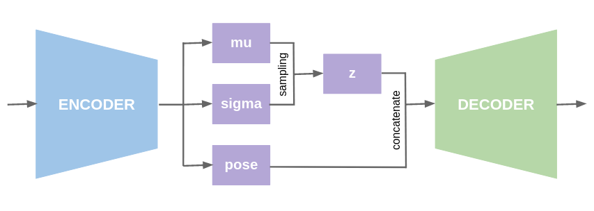
Figure 1: Architecture of the affinity-VAE.

The cosine similarity measures the distance between two latent points, whereas the pre-computed affinity matrix ($\mathbf{A}$) provides feedback on their actual pairwise similarity. This effectively organises the latent space so that similar objects (regardless of their pose), as described by the similarity descriptor in the affinity matrix, are placed close together in the latent space. The pre-calculated affinity matrix is generated automatically by computing pairwise similarity scores for the entire training dataset with a target function. In our case this is SOAP for the 2D alphanumeric data and FSC for 3D protein data (more on data generation in section 2.5), but different metrics could be chosen to facilitate different datasets, or to organise the latent space by different factors (see section 2.6). Furthermore, the affinity matrix is only used in the training stage, therefore a pre-trained network can be easily applied to discovery of new classes/species.

2.2.2 Pose channel

The latent space is represented in terms of distributions expressed through learnable fully connected layers for the mean ($\mu$) and the variance ($\sigma$). We have introduced a third learnable fully connected layer to represent the $n$-D pose of the object, in a similar manner to rotation in an rVAE [4, 30]. By feeding the same shape similarity values (matrix identity) for the same object regardless of its orientation, we force the latent space and the additional pose parameter to learn to represent the pose of the object.

2.3 Latent map

To ensure that our method is generalising to new data/tomograms so that the network does not need retraining every time it analyses new data, we introduce the "latent map" approach. Instead of training the network on the whole tomogram, we create a latent "map" pre-seeded with existing proteins. Once pre-trained with a set of objects that is non-redundant (i.e. no duplicates) but exhaustive (i.e. considering all morphologies), the latent space can be used as a dictionary or a reference space for both seen and unseen data. The seen data would form clusters within or near the existing cluster centres in the latent map while the unseen data would do so near or between groups of similar morphology. This brings in a promise of applying affinity-VAE as an unsupervised template-and-label-free approach to the classification and detection of unseen samples or novel structures in cryo-ET tomograms.

2.4 Latent embeddings, clustering and KNN

The encoded samples are represented in the latent space through their generative factors, however the dimensionality of that latent space ($z$) is a hyperparameter. We are therefore analysing $n$-D latent spaces such that $n$ is high enough to capture the complexity in the original image, but low enough to only capture the true semantics. Therefore, even with the simplest 3D datasets $n>2$. To visualise and interpret any relationships between the latent codes corresponding to different semantics, and visually assess the degree to which identical or similar objects form homogeneous clusters in the latent space, we produce latent embeddings in which each latent vector is given a location in a lower-dimensional (2D) manifold. We have explored the following methods for visualisation of latent embeddings:

• UMAP [33] (Uniform Manifold Approximation and Projection) – used for our 2D alphanumeric data;

• t-SNE [34] (t-Distributed Stochastic Neighbour Embedding) – used for our 3D protein and tetramino data.

The accuracy of the method was evaluated in three different ways. To assess whether the object was classified correctly we explored the following approaches:

• means for the clusters are calculated and each point is classified to belong in a cluster if it lies within +/- $2\sigma$ of the mean - used for 2D alphanumeric data;

• $k=5$ nearest neighbors (KNN) [35] were selected for each encoded data point and a class was assigned based on majority voting (producing hard assignments) – used for 3D protein and tetramino data;

• $k=100$ nearest neighbors [35] were selected and assignment fractions for each class were used as likelihood of belonging to that class (producing soft probabilistic assignments) – used for 3D protein and tetramino data.

For quick evaluation of the 3D data we used hard assignments because they are faster, however soft assignments provide more insight into the classification, which is particularly useful for evaluating unseen data or novel structures.

2.5 Data simulation

Three datasets were used in the evaluation of the methods: 1) 2D alphanumeric data, 2) 3D tetramino data, and 3) simulated 3D protein data.

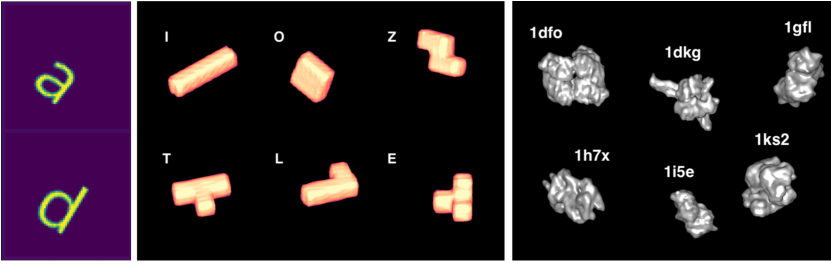
Figure 2: Sample data, left: alphanumeric, middle : tetramino blocks and right: protein volumes from the list in [36].

Images in the alphanumeric dataset are constructed from letters and digits ($x\in\{\texttt{a, e, b, d, p, i, j, z, 2, k, x, u}\}$), rotated at various angles (Figure 2 left). Images are created using the Pillow library in Python [37], rotated to a defined angle $\theta$ where $\left\{\theta\in\mathbb{Z}|-45<\theta<45\right\}$, and converted to a binary two-dimensional array. We use an $80/20$ split for training and testing.

The tetramino data (Figure 2 middle) was designed to emulate an easier, but similar, 3D scenario to real cryo-ET data. Tetraminos were made of combinations of four identical cubes connected wall-to-wall. They were generated on-the-fly with controllable parameters such as rotation and translation. Other controllable aspects include morphological adjustments (e.g. elongation) to test the semantic disentangling power of the method. This allows us to generate any desired shape combinations to fully test the performance of our method. The training data was constructed from 6 morphologically different tetraminos which were used to pre-seed the latent map, while for evaluation we constructed a new, previously unseen class that was morphologically similar to two other classes from the training set. All data was augmented using rotations randomly sampled at $\theta=\{10,20,...,360\}$ in 3 different planes. All images were resized prior to training to 32x32x32 voxels. Test and validation data constituted 10% and 20% of the training set respectively.

The protein data (Figure 2 right) was generated from the list of 50 most abundant E. coli proteins [36]. Chimera [38] was used to generate a synthetic 3D density map from each protein on the list. The maps were generated at 10 Å resolution without taking atomic $B$-factors into account. The training data was constructed from $n$ randomly selected classes (protein types), which were used to pre-seed the latent map, and a different, previously unseen class was selected for evaluation. All data was augmented with rotations randomly sampled at $\theta=\{10,20,...,360\}$ in 3 different planes. All images were resized prior to training to 64x64x64 voxels. Test and validation data constituted 10% and 20% of the whole dataset respectively.

2.6 Affinity metrics

Regularisation of the latent space ensures that semantically similar objects are encoded near to each other (i.e. at similar positions in latent space) while dissimilar objects are encoded far apart. To achieve this regularisation we require knowledge of the similarity between all pairs of training examples. The affinity between two structures can be described in accordance with the intrinsic properties of the data. The choice of affinity descriptor (shape, or indeed any other metric) should therefore be made with respect to the property of the data intended to achieve the desired data separation.

2.6.1 2D alpha-numeric data

In order to investigate the similarity between two structures in the alphanumeric data, we employ the Smooth Overlap of Atomic Positions (SOAP) descriptor [39, 40]. This shape descriptor uses a combination of radial and spherical harmonics. In our model, we are treating every pixel that is not background as an “atom”. The SOAP descriptor places a Gaussian density distribution at the location of each selected pixel. The SOAP kernel is then defined as the overlap of the two local nearest neighbouring densities integrated over all three-dimensional rotations.

2.6.2 3D tetramino and protein data

Fourier shell correlation (FSC) [26] curves are the standard metric for resolution estimation of cryo-EM maps. The method calculates the similarity of two images as a function of spatial frequency, by calculating the correlation between the Fourier coefficients of each image in thin spherical shells:

$$FSC(k)=\frac{\sum{F_{1}(k)F_{2}(k)^{*}}}{\sqrt{\sum{|F_{1}(k)|^{2}}\sum{|F_{2}(k)|^{2}}}}$$ (4)

where $F_{1}(k)$ and $F_{2}(k)$ are the (complex) coefficients of the Fourier transforms of the two structures in a spherical shell at radius $k$. In this work, to obtain a single value for use as an affinity metric, we take an average of the FSC across all spatial frequency shells, weighted by the number of Fourier coefficients in each shell according to the method described by Brown et al. [41]. This gives a measure of similarity between the two 3D objects with a value between $+1$ and $-1$, with the former indicating a strong agreement.

3 Results

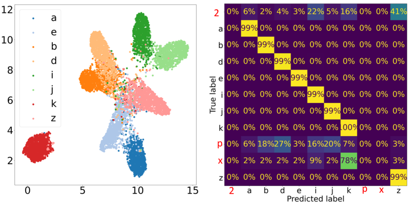
Figure 3: Left: UMAP embedding of latent space trained with 10000 randomly rotated samples of alphanumeric data. Right: The confusion matrix build from the prediction for 200 samples of seen (a, b, d, e, i, j, z and k) and unseen data (2, x and p). For this calculation the choice of hyperparameters include $\gamma=8$ and $\beta=5$.

3.1 Latent clustering for 2D alpha-numeric data

Given the appropriate choice of hyper-parameters, data classes are clustered together for the alphanumeric data in the latent space and the clusters are correlated in accordance to their shape. The left panel of Figure 3 illustrates the UMAP embedding of 10,000 rotations from a set of samples from the alphanumeric data. For this calculation the choice of hyperparameters include $\gamma=8$ and $\beta=5$. The right panel shows the confusion matrix constructed from the prediction for 200 samples of the seen data (a, b, d, e, i, j, z and k) and unseen data (2, x and p). The confusion matrix shows that the model predicts a strong affinity between letters with higher shape similarity for the seen and unseen data (for example, the unseen numeral 2 shows the closest match to the letter z from the training set).

3.2 Latent clustering for 3D tetramino and protein data

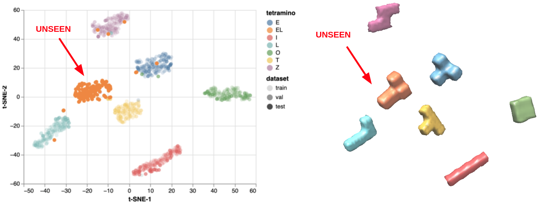
Figure 4: Left: t-SNE embedding of 1000 (rotationally augmented) tetraminos from a set of morphologies. Different colours correspond to different morphologies and opacity indicates train/validation/test set. Right: Morphology of different tetramino types positioned in areas corresponding to their latent location. Colors between left and right panel are corresponding. Tetramino unseen during training and validation indicated with red arrow.

The results on the tetramino data are illustrated in the latent embedding in Figure 4 and on the protein data in the latent embedding in Figure 5. In both datasets, the cluster separation between different morphologies was very good. Rotated objects of the same morphology were placed in homogeneous clusters regardless of their orientation. Additionally, in the tetramino data the clusters were arranged so that morphologically similar objects (e.g. E and T, L and I) were closer together in the latent space than dissimilar objects (e.g. I and E). A similar trend was observed in the protein data, where dimeric (two subunit) proteins were all arranged close together and ordered by the size of the protein, whereas elongated monomeric (single-subunit) proteins were placed separately forming a more homogeneous area in the latent space.

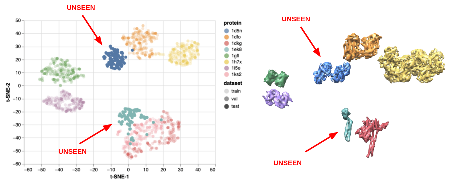
Figure 5: Left: t-SNE embedding of 1000 (rotationally augmented) proteins from a set of 8 randomly chosen morphologies. Different colours correspond to different morphologies and opacity indicates train/validation/test set. Right: Morphology of different protein types positioned in areas corresponding to their latent location. Colors between left and right panel are corresponding. Proteins unseen during training and validation indicated with red arrows.

When the network was presented with samples previously unseen during training, they formed separate clusters in the embedding positioned close to similar morphologies, which suggests that the learned latent spaces are continuous (see more in subsection 3.3) and offers potential use of the method for discovery of new morphologies. At the same time, cluster homogeneity was preserved within the unseen clusters, regardless of the object orientation. In the case of the tetramino data, we introduced a new morphology during evaluation that was a fusion of two similar morphologies existing in training (EL), which, as expected, clustered between the two similar classes (E and L). In the case of the protein data, the two introduced morphologies were selected randomly from a list containing an exhaustive set of proteins from the E. coli cytoplasm. The dimeric protein (blue) was placed near other dimers and positioned in a roughly correct position arranged by size (increasing left to right). The monomeric protein with an elongated domain was placed overlapping with another cluster of proteins with elongated domains.

The accuracy of classification as measured by KNN on the protein test set was up to 90% with the optimal set of hyperparameters.

3.3 Latent and pose interpolations

We performed interpolations across the outputs of the pose channel on alphanumeric data. The results of the interpolations are illustrated in Figure 6. We observed a linear correlation between the pose value and the angle of the rotation, which demonstrates that pose channel does indeed capture information about the pose of the object.

We also explored the extent of disentanglement present in the generated latent spaces. Upon visual inspection we were able to identify morphological semantics across different dimensions (Figure 7 left). In this example using the protein data, dimension 2 appeared to capture the size, whereas dimension 6 described whether the protein was a dimer (two subunits) or a monomer (single unit). Other dimensions supported other morphological features, including elongation (dim 1), smoothness (dim 3 and 4), and toroidal geometry (dim 5).

Additionally, we performed latent interpolations across all dimensions between four existing (encoded) data points in the latent space (Figure 7 right). Non-existing (not encoded) points from the latent space generated realistic reconstructions and there was a smooth transition between different morphologies, including when transitioning between the number of protein subunits. This shows that the generated latent spaces are continuous and suitable to discovery of new morphologies unseen during training.

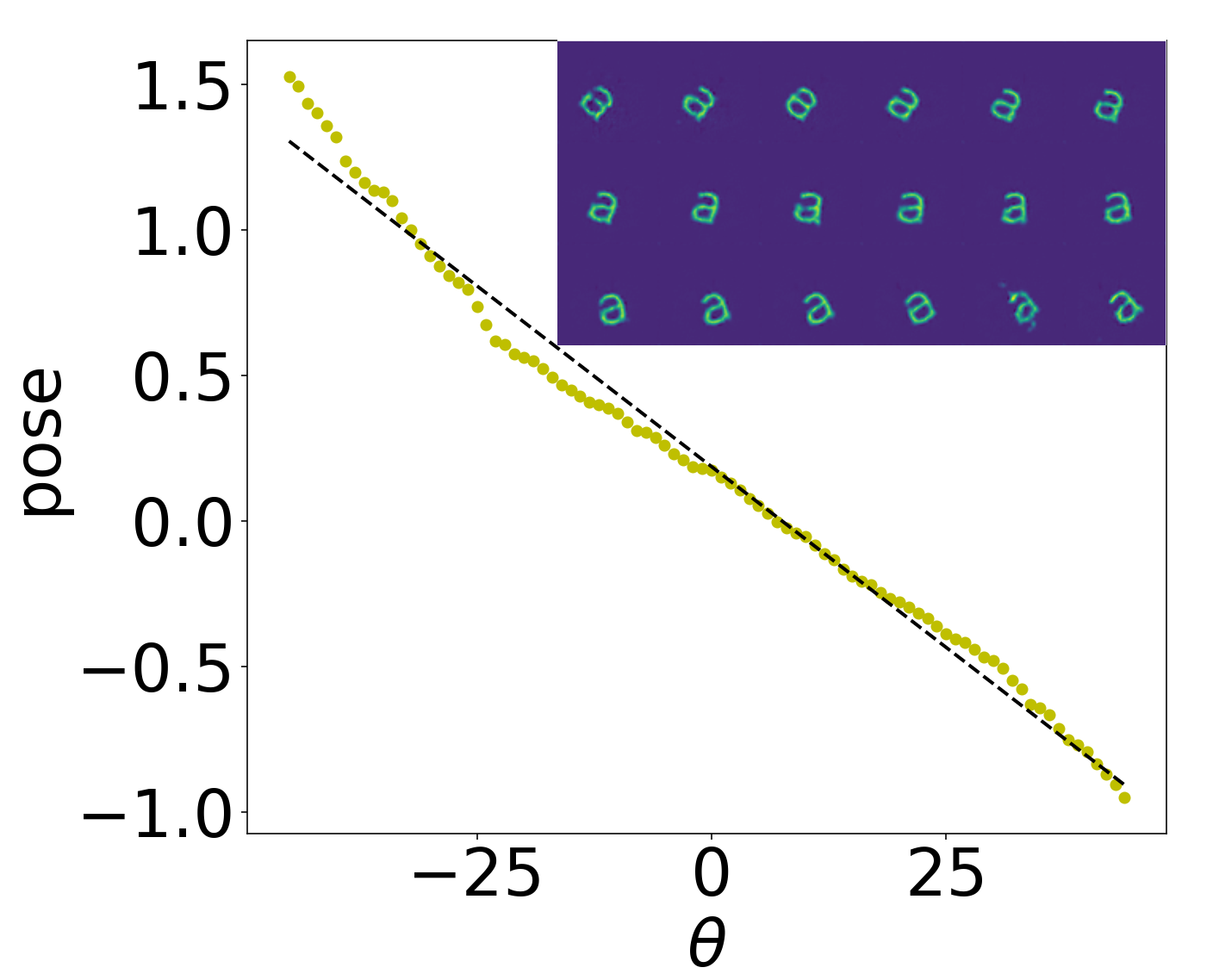
Figure 6: Linear relationship between encoded pose and the associated angle of rotation of the input. The nested panel shows the reconstruction using a given latent encoding ($z$) and varying the value of the pose corresponding to 5 degree intervals.

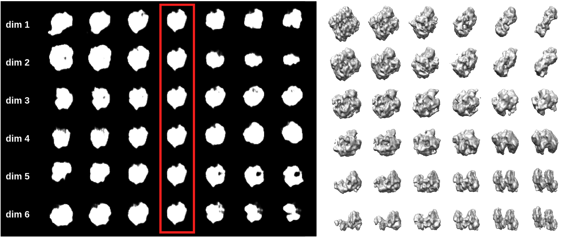
Figure 7: Left: Latent interpolations on protein data in a 6 dimensional latent space. Rows correspond to dimensions and columns correspond to interpolated values, where the central column is the encoded input. Right: Latent interpolations between 4 existing encoded proteins (corners). Decoded reconstructions in between the 4 corners are taken from the latent space at evenly sampled multi-dimensional strides between the encodings of existing proteins.

3.4 Affinity-based loss component and the influence of $\gamma$

Figure 8 illustrates a comparison between affinity-VAE and a standard $\beta$-VAE ($\gamma=0$ and no pose channel) on alphanumeric data, including the latent space representations (top row) as well as the proximity matrix where the distances between the centres of the clusters are displayed (bottom row). Inspection of the two latent space representations shows that affinity-VAE ($\gamma=10$) is more successful at relating the clusters with higher affinity than the $\beta$-VAE framework ($\gamma=0$). This is confirmed in the proximity matrix where the distances between different clusters (i.e. the off-diagonal elements) are generally much higher in affinity-VAE than in the $\beta$-VAE, which would be expected to improve classification rates due to less cluster proximity contamination. Secondly, letters with similar morphology (e.g. b and d) are in closer proximity in the latent map in affinity-VAE compared with $\beta$-VAE. Another example of this is the proximity of cluster i and j to cluster z in $\beta$-VAE, which have been pushed apart in affinity-VAE due to the low affinity.

When $\gamma$ was set to 0 and pose turned off on protein data, the resulting latent spaces generated by the standard $\beta$-VAE were still organised, however the organisation was by an offset from the centre (radially) and an average intensity (within each cluster) of the object (Figure 9) rather than morphological affinity (as previously demonstrated in Figure 5). Since $\beta$-VAE is completely data-agnostic, we have little control over the learned factorised representations and the semantics we want to capture.

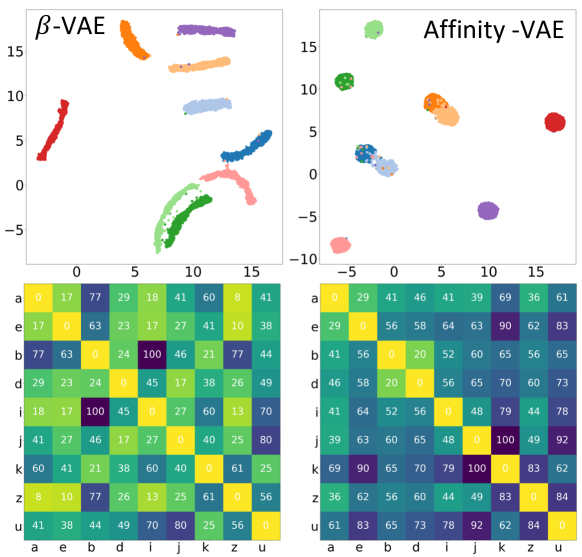
Figure 8: Latent space representation for the alphanumeric dataset using VAE where $\gamma=0$ and pose channel is off (left column) and affinity-VAE where $\gamma=10$ (right column). Bottom row: latent space proximity matrix displaying the distance between cluster centres. The values for the distances in the are normalised to be between 0-100 in both matrices. The colour map is used as a guide for the eye to emphasise the largest and smallest numbers displayed on the matrix.

Introducing the affinity matrix and a similarity-based loss component organises the latent space by the quality captured through the similarity metric.

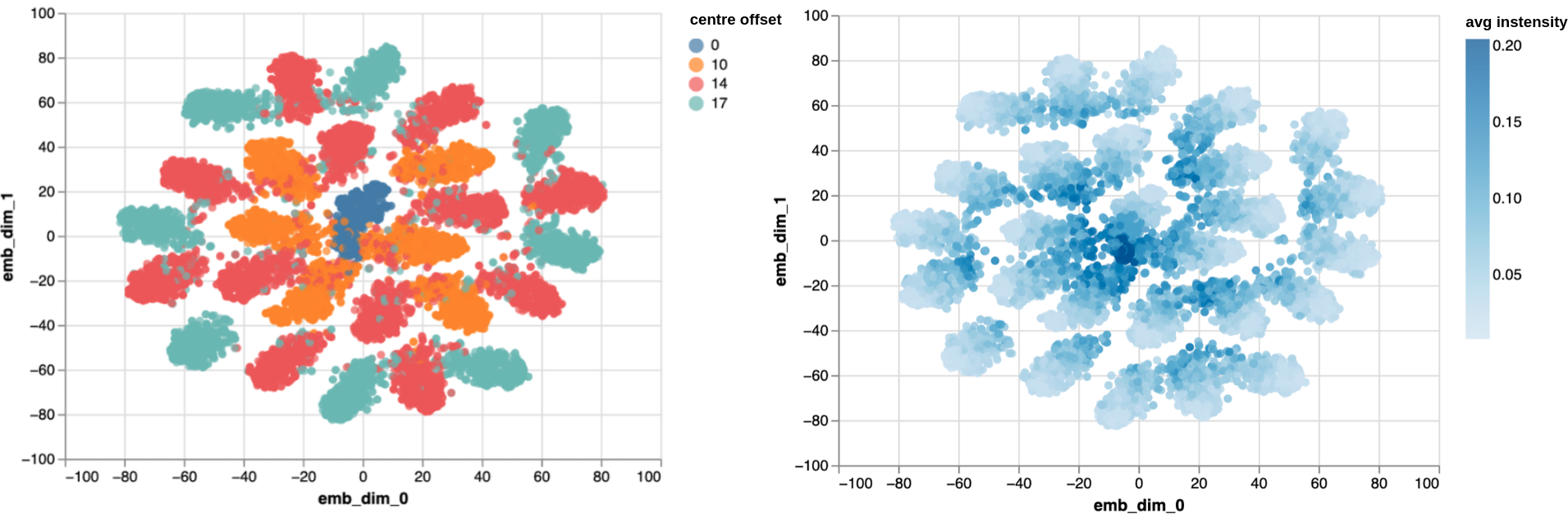
Figure 9: Latent embedding on a tetramino data from a hyperparameter-tuned $\beta$-VAE ($\gamma=0).$ The latent space is organised by centre offset radially (left) and average intensity within clusters (right).

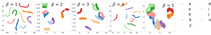
Figure 10: The latent space is presented for $\beta=1,2,3,4$ and $5$ using original VAE framework ($\gamma=0$). A more effective categorisation of classes is observed for values $\beta>1$.

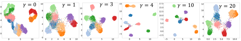
Figure 11: For $\beta=5$ we have explored the effect of shape-affinity regularisation of latent space for $\gamma=0,1,3,4,6,10$ and $20$. The colour code is the same as Figure 10.

3.5 The influence of $\beta$, $\gamma$ and $z$

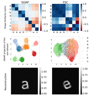
Figure 12: The left and right panel show a comparison of the latent space representation and the reconstruction of the alphanumeric data for the SOAP and FSC shape descriptors respectively.

In order to achieve an appropriately disentangled latent representation, the value of $\beta$ should be chosen carefully. Since $\beta=1$ corresponds to the original VAE method, a stronger emphasis on the $D_{KL}$ term ($\beta>1$ in our case) encourages learning of a more disentangled latent representation as shown in Figure 10. This is in agreement with existing literature [2, 32]. Within the affinity-VAE framework, the value of $\gamma$ should be chosen in a similar range to that of $\beta$. This is due to the competing effect of the two terms in Equation 2.

Figure 11 explores the effect of affinity regularisation on the latent space. By switching on the shape-affinity ($\gamma>0$) the clusters are instantly grouped together based on their shape-similarity unlike the $\beta$-VAE framework where the letters do form clusters of their own, but are not closer in the latent space if they are similar in shape (Figure 10). As the emphasis on the affinity increases, the latent space becomes increasingly sparse pushing the clusters further apart. The suitability of this empty space for specific studies can be explored by investigating the continuity through latent interpolations and classification of unseen data.

For tetraminos, the optimal range of latent dimensions was between 5 and 9. We also observed a relationship between the number of dimensions and degrees of freedom in the data (e.g. 3 rotations, translations + semantics). Small values of $\beta$ (but $>1$) gave best accuracy. Increasing the affinity regularisation $\gamma$ produced better KNN accuracy (saturated around value of 1000), however, it also increased reconstruction loss. This is expected, as latent regularisation vs. reconstruction quality is always a trade-off, and in our case latent disentanglement (and therefore accurate classification and recognition) is more important than faithful reconstructions.

3.6 Similarity function

To illustrate the influence of the choice of similarity metric used to calculate the affinity matrix on the overall cluster separation we compared various metrics across different datasets.

While the SOAP metric was used for 2D alphanumeric data and FSC for 3D data, a comparison between the two descriptors for the alphanumeric data is provided in Figure 12. SOAP provided better cluster separation as well as increased certainty of reconstruction on the alphanumeric data.

We also explored the choice of similarity metric in 3D tetramino data. Figure 13 shows a comparison between no affinity descriptor, mean difference and FSC metrics. Mean difference, unlike avg FSC, is a real space descriptor which is not frequency weighted (Equation 5).

$$\frac{1}{N}\sum_{i=0}^{i=N}x_{i}-y_{i}$$ (5)

where $x_{i}$ and $y_{i}$ are voxels in comparison, and $N$ stands for the number of voxels (image size).

While mean difference also improved the cluster separation over a standard $\beta$-VAE, some clusters (e.g. L and I) still remained joint. On the other hand, after employing the FSC as a similarity metric not only did the cluster separation improve, but also the organisation of clusters was morphologically aligned (e.g. elongated shapes like L, I and T clustered near each other).

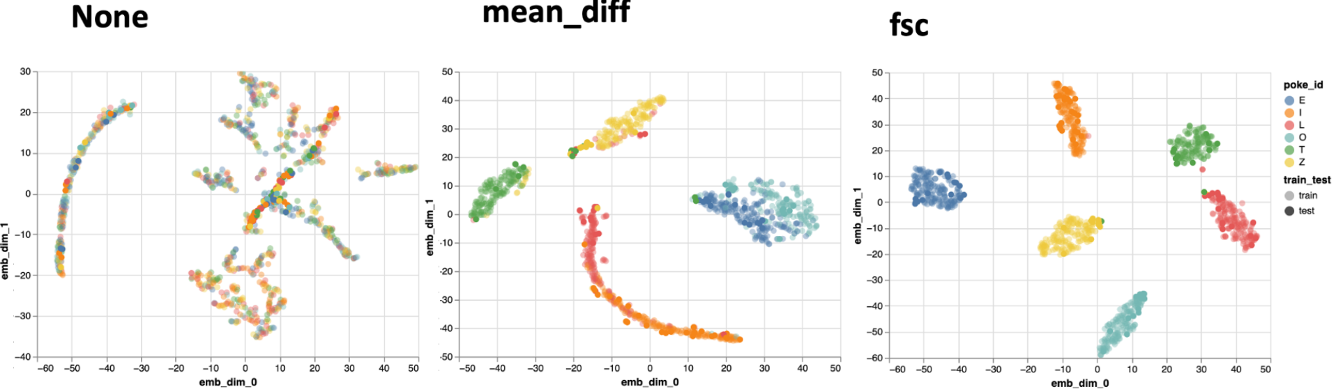
Figure 13: The left, middle and right panel show a comparison of the t-SNE latent space embeddings for the tetramino data for no affinity descriptor, mean difference and FSC respectively.

4 Discussion

In this work we have introduced affinity-VAE, a neural network capable of organising the latent representation based on the similarity of the object. While a $\beta$-VAE is capable of cluster separation and latent disentanglement, we have little control over the learned factorised representations and captured semantics. We have shown that with guidance from an automatically generated affinity matrix we can create more homogeneous, rotationally-invariant clusters that could improve the classification accuracy. Furthermore, the affinity metric can be tailored to the data or domain of interest, improving the generality of the method. Since the affinity metric is only utilised during the training phase (Equation 2), we can infer the similarity of unseen objects in the encoded latent representation. A pre-trained network can therefore be easily applied to discovery of new classes. We have demonstrated that the learned latent spaces can be continuous, which enables the potential use of the method with unseen data (e.g. discovery of new species).

We have demonstrated the potential of the method in a scientific application using the example of subtomogram target identification in volumetric cryo-ET data. While the results are promising and show the potential of the method for discovery of new species in experimental data, more experiments are required to test the effectiveness of the method on a full tomogram. This comes with new challenges, notably the presence of noise, crowding, interactions, multiple conformations and translation.

References

- [1] D. P. Kingma and M. Welling, “Auto-encoding variational bayes,” International Conference on Learning Representations (ICLR) 2014, 2014.
- [2] I. Higgins, L. Matthey, A. Pal, C. Burgess, X. Glorot, M. Botvinick, S. Mohamed, and A. Lerchner, “beta-VAE: Learning basic visual concepts with a constrained variational framework,” 2017.
- [3] T. Bepler, E. Zhong, K. Kelley, E. Brignole, and B. Berger, “Explicitly disentangling image content from translation and rotation with spatial-vae,” Advances in Neural Information Processing Systems, vol. 32, 2019.
- [4] M. Ziatdinov, A. Ghosh, T. Wong, and S. V. Kalinin, “Atomai: A deep learning framework for analysis of image and spectroscopy data in (scanning) transmission electron microscopy and beyond,” arXiv preprint arXiv:2105.07485, 2021.
- [5] A. Huth, S. Nishimoto, A. Vu, and J. Gallant, “A continuous semantic space describes the representation of thousands of object and action categories across the human brain,” Neuron, vol. 76, no. 6, pp. 1210–1224, 2012.
- [6] H. P. Op de Beeck, K. Torfs, and J. Wagemans, “Perceived shape similarity among unfamiliar objects and the organization of the human object vision pathway,” Journal of Neuroscience, vol. 28, no. 40, pp. 10111–10123, 2008.
- [7] C. M. Oikonomou, Y.-W. Chang, and G. J. Jensen, “A new view into prokaryotic cell biology from electron cryotomography,” Nature Reviews Microbiology, vol. 14, no. 4, pp. 205–220, 2016.
- [8] F. J. Bäuerlein and W. Baumeister, “Towards visual proteomics at high resolution,” Journal of Molecular Biology, vol. 433, no. 20, p. 167187, 2021.
- [9] A. Sali, R. Glaeser, T. Earnest, and W. Baumeister, “From words to literature in structural proteomics,” Nature, vol. 422, no. 6928, pp. 216–225, 2003.
- [10] M. Turk and W. Baumeister, “The promise and the challenges of cryo-electron tomography,” FEBS Letters, vol. 594, no. 20, pp. 3243–3261, 2020.
- [11] K. Murata, X. Liu, R. Danev, J. Jakana, M. F. Schmid, J. King, K. Nagayama, and W. Chiu, “Zernike phase contrast cryo-electron microscopy and tomography for structure determination at nanometer and subnanometer resolutions,” Structure, vol. 18, no. 8, pp. 903–912, 2010.
- [12] L. Jin, A.-C. Milazzo, S. Kleinfelder, S. Li, P. Leblanc, F. Duttweiler, J. C. Bouwer, S. T. Peltier, M. H. Ellisman, and N.-H. Xuong, “Applications of direct detection device in transmission electron microscopy,” Journal of structural biology, vol. 161, no. 3, pp. 352–358, 2008.
- [13] W. Kühlbrandt, “The resolution revolution,” Science, vol. 343, pp. 1443–1444, mar 2014.
- [14] W. Wan and J. A. Briggs, “Cryo-electron tomography and subtomogram averaging,” Methods in enzymology, vol. 579, pp. 329–367, 2016.
- [15] D. Castaño-Díez and G. Zanetti, “In situ structure determination by subtomogram averaging,” Current Opinion in Structural Biology, vol. 58, pp. 68–75, oct 2019.
- [16] W. Wan and J. Briggs, “Cryo-electron tomography and subtomogram averaging,” in Methods in Enzymology, pp. 329–367, Elsevier, 2016.
- [17] K. Y. Foo, K. Newman, Q. Fang, P. Gong, H. M. Ismail, D. D. Lakhiani, R. Zilkens, B. F. Dessauvagie, B. Latham, C. M. Saunders, L. Chin, and B. F. Kennedy, “Multi-class classification of breast tissue using optical coherence tomography and attenuation imaging combined via deep learning,” Biomed. Opt. Express, vol. 13, pp. 3380–3400, Jun 2022.
- [18] M. Kavitha, N. Yudistira, and T. Kurita, “Multi instance learning via deep cnn for multi-class recognition of alzheimer’s disease,” in 2019 IEEE 11th International Workshop on Computational Intelligence and Applications (IWCIA), pp. 89–94, 2019.
- [19] T. Bepler, A. Morin, M. Rapp, J. Brasch, L. Shapiro, A. J. Noble, and B. Berger, “Positive-unlabeled convolutional neural networks for particle picking in cryo-electron micrographs,” Nature Methods, vol. 16, pp. 1153–1160, oct 2019.
- [20] T. Wagner, F. Merino, M. Stabrin, T. Moriya, C. Antoni, A. Apelbaum, P. Hagel, O. Sitsel, T. Raisch, D. Prumbaum, D. Quentin, D. Roderer, S. Tacke, B. Siebolds, E. Schubert, T. R. Shaikh, P. Lill, C. Gatsogiannis, and S. Raunser, “SPHIRE-crYOLO is a fast and accurate fully automated particle picker for cryo-EM,” Communications Biology, vol. 2, jun 2019.
- [21] E. Palovcak, D. Asarnow, M. G. Campbell, Z. Yu, and Y. Cheng, “Enhancing the signal-to-noise ratio and generating contrast for cryo-EM images with convolutional neural networks,” IUCrJ, vol. 7, pp. 1142–1150, Nov 2020.
- [22] E. Moebel, A. Martinez-Sanchez, L. Lamm, R. D. Righetto, W. Wietrzynski, S. Albert, D. Larivière, E. Fourmentin, S. Pfeffer, J. Ortiz, et al., “Deep learning improves macromolecule identification in 3d cellular cryo-electron tomograms,” Nature methods, vol. 18, no. 11, pp. 1386–1394, 2021.
- [23] B. Chidester, T. Zhou, M. N. Do, and J. Ma, “Rotation equivariant and invariant neural networks for microscopy image analysis,” Bioinformatics, vol. 35, pp. i530–i537, 07 2019.
- [24] V. Delchevalerie, A. Bibal, B. Frenay, and A. Mayer, “Achieving rotational invariance with bessel-convolutional neural networks,” in Advances in Neural Information Processing Systems (A. Beygelzimer, Y. Dauphin, P. Liang, and J. W. Vaughan, eds.), 2021.
- [25] X. Min, I. Tocheva Elitza, C. Yi-Wei, J. Jensen Grant, and A. Frank, “De novo visual proteomics in single cells through pattern mining,” arXiv preprint arXiv:1512.09347, 2015.
- [26] G. Harauz and M. van Heel, “Exact filters for general geometry three dimensional reconstruction.,” Optik., vol. 73, no. 4, pp. 146–156, 1986.
- [27] G. Rice, T. Wagner, M. Stabrin, and S. Raunser, “TomoTwin: Generalized 3d localization of macromolecules in cryo-electron tomograms with structural data mining,” jun 2022.
- [28] E. D. Zhong, T. Bepler, B. Berger, and J. H. Davis, “Cryodrgn: reconstruction of heterogeneous cryo-em structures using neural networks,” Nature Methods, vol. 18, no. 2, pp. 176–185, 2021.
- [29] X. Zeng, M. R. Leung, T. Zeev-Ben-Mordehai, and M. Xu, “A convolutional autoencoder approach for mining features in cellular electron cryo-tomograms and weakly supervised coarse segmentation,” Journal of structural biology, vol. 202, no. 2, pp. 150–160, 2018.
- [30] M. Ziatdinov and S. Kalinin, “Atomai: Open-source software for applications of deep learning to microscopy data,” Microscopy and Microanalysis, vol. 27, no. S1, p. 3000–3002, 2021.
- [31] T. Chen, S. Kornblith, M. Norouzi, and G. Hinton, “A simple framework for contrastive learning of visual representations,” in International conference on machine learning, pp. 1597–1607, PMLR, 2020.
- [32] C. P. Burgess, I. Higgins, A. Pal, L. Matthey, N. Watters, G. Desjardins, and A. Lerchner, “Understanding disentangling in -VAE,” CoRR, vol. abs/1804.03599, 2018.
- [33] L. McInnes, J. Healy, and J. Melville, “Umap: Uniform manifold approximation and projection for dimension reduction,” arXiv preprint arXiv:1802.03426, 2018.
- [34] L. Van der Maaten and G. Hinton, “Visualizing data using t-sne.,” Journal of machine learning research, vol. 9, no. 11, 2008.
- [35] N. S. Altman, “An introduction to kernel and nearest-neighbor nonparametric regression,” The American Statistician, vol. 46, no. 3, pp. 175–185, 1992.
- [36] S. R. McGuffee and A. H. Elcock, “Diffusion, crowding & protein stability in a dynamic molecular model of the bacterial cytoplasm,” PLOS Computational Biology, vol. 6, pp. 1–18, 03 2010.
- [37] A. Clark, “Pillow (pil fork) documentation,” 2015.
- [38] E. F. Pettersen, T. D. Goddard, C. C. Huang, G. S. Couch, D. M. Greenblatt, E. C. Meng, and T. E. Ferrin, “Ucsf chimera—a visualization system for exploratory research and analysis,” Journal of computational chemistry, vol. 25, no. 13, pp. 1605–1612, 2004.
- [39] A. P. Bartók, M. C. Payne, R. Kondor, and G. Csányi, “Gaussian approximation potentials: The accuracy of quantum mechanics, without the electrons,” Phys. Rev. Lett., vol. 104, p. 136403, Apr 2010.
- [40] A. P. Bartók, R. Kondor, and G. Csányi, “On representing chemical environments,” Phys. Rev. B, vol. 87, p. 184115, May 2013.
- [41] A. Brown, F. Long, R. A. Nicholls, J. Toots, P. Emsley, and G. Murshudov, “Tools for macromolecular model building and refinement into electron cryo-microscopy reconstructions,” Acta Crystallographica Section D: Biological Crystallography, vol. 71, no. 1, pp. 136–153, 2015.