Time-domain modeling of interband transitions in plasmonic systems

Abstract

Efficient modeling of dispersive materials via time-domain simulations of the Maxwell equations relies on the technique of auxiliary differential equations. In this approach, a material’s frequency-dependent permittivity is represented via a sum of rational functions, e.g. Lorentz-poles, and the associated free parameters are determined by fitting to experimental data. In the present work, we present a modified approach for plasmonic materials that requires considerably fewer fit parameters than traditional approaches. Specifically, we consider the underlying microscopic theory and, in the frequency domain, separate the hydrodynamic contributions of the quasi-free electrons in partially filled bands from the interband transitions. As an illustration, we apply our approach to Gold and demonstrate how to treat the interband transitions within the effective model via connecting to the underlying electronic bandstructure, thereby assigning physical meaning to the remaining fit parameters. Finally, we show how to utilize this approach within the technique of auxiliary differential equations. Our approach can be extended to other plasmonic materials and leads to efficient time-domain simulations of plasmonic structures for frequency ranges where interband transitions have to be considered.

1 Introduction

In macroscopic electrodynamics at near-IR or optical frequencies, linear material properties are commonly described by frequency-dependent permittivities $\epsilon(\omega)$. Their experimental determination happens, e.g., by means of ellipsometry [1] and the so-obtained data can directly be fed into computational approaches that solve Maxwell’s equations in the frequency domain. Their incorporation into time-domain Maxwell-solvers requires more effort because, in the time domain, the constitutive relation $\vec{D}(\omega)=\epsilon_{0}\epsilon(\omega)\vec{E}(\omega)$ translates to a convolution integral, thus turning Maxwell’s equations into a set of numerically demanding integro-differential equations. Here, $\epsilon_{0}$ denotes the vacuum permittivity.
Within the framework of auxiliary differential equations (ADEs), this convolution integral is circumvented and replaced by a set of differential equations for auxiliary polarizations or auxiliary currents. This is accomplished by writing the permittivity as a sum of rational functions in $\omega$ that respect appropriate Kramers-Kronig relations in order to ensure causality [2] (for concrete examples of ADEs, see section 3.1 below). For instance, metals are often treated via the so-called Drude-Lorentz model

$$\epsilon(\omega)=1-\frac{\omega_{p}^{2}}{\omega(\omega+i\gamma_{\rm D})}+\sum_{m=1}^{N}\frac{f_{m}\omega_{p}^{2}}{\omega_{m}^{2}-\omega^{2}-i\omega\gamma_{m}}.$$ (1)

Here, the 1st and 2nd term on the r.h.s. represent, respectively, the vacuum contribution and the (collective) response of the metal’s free electrons, the so-called Drude model with plasma frequency $\omega_{p}$ and phenomenological damping constant $\gamma_{\rm D}$.
In dielectrics, the 3rd term on the r.h.s. of Eq. (1) models electrons that are elastically bound to their parent nuclei so that the $f_{m}$ and $\omega_{m}$ $(m=1,\dots,N)$ may be interpreted, respectively, as oscillator strengths and frequencies of corresponding chemical bonds or may be associated with certain transitions in the electronic bandstructure of semiconductors. This particular form of the linear response has been suggested on empirical grounds by Sellmeier in 1871 [3], albeit for different reasons. In addition, a set of phenomenological damping constants $\gamma_{m}$ $(m=1,\dots,N)$ are introduced. As a result, each Lorentz pole features three adjustable parameters that are obtained from fits to experimental permittivity data, where the oscillator strengths obey a sum rule. Often, additional frequency dependencies are associated to the damping constants [4].
In metals, Lorentz poles are used to account for interband transitions so that $f_{m}$, $\omega_{m}$, and $\gamma_{m}$ ($m=1,\dots,N$) and the number $N$ of Lorentz poles represent effective parameters without straightforward physical interpretation. Nonetheless, sophisticated and rather cumbersome methods [5] have been developed to fit the parameters of the Drude-Lorentz model, Eq. (1), to experimental data such as those provided by the classic measurements of Johnson & Christy for noble metals [6] or the data reported in the handbook of optical constants of solids edited by Palik [7].
In the present work, we adopt a more microscopic viewpoint on $\epsilon(\omega)$ and demonstrate (i) how this leads to a considerable reduction in the number of fit parameters and (ii) how the remaining parameters may be interpreted physically. Further, our approach provides an alternative perspective on Eq. (1) and offers a systematic way of improving the accuracy of time-domain computations without introducing additional fit parameters. Our work is organized as follows. In section 2, we review some of the available literature, develop our approach, and apply it to the permittivity of gold, the perhaps most frequently used plasmonic material. We proceed in section 3 to the adaptation of our approach for time-domain simulations and provide numerical assessments of its validity. In section 4, we summarize our findings.

2 Theory of the frequency-dependent permittivity of metals

One of the earliest discussion on the permittivity of metals dates back to two works of Darwin [8, 9]. There, on a classical level, it was explained that the bound and free electron response are additive and that there is no local field correction in a plasma. On the quantum mechanical level, Bohm and Pines [10, 11, 12, 13] have elaborated the physical properties of metals. Regarding the metals’ response to electromagnetic fields [12], they have demonstrated that the complicated multi-particle interactions in a metal can be classified into two types which require rather distinct treatments. More precisely, there exist collective excitations of the electron system that are dominant at long wavelengths and that can be treated via Fermi-liquid theory (Landau-Silin theory [14]) where the periodic (i.e. atomic) nature of the ionic background is essentially irrelevant. Through a corresponding canonical transformation of the original Hamiltonian, the remaining short-range interactions are then mapped onto a collection of independent particles that move in an effective periodic potential. Consequently, this separation of spatial scales leads to a description of the electron system as a mixture of a Fermi liquid and a set of non-interacting effective particles.
It is to this mixture that the aforementioned arguments of Darwin may be applied so that the linear permittivity of metals may be decomposed into

$$\epsilon_{\rm Metal} =1+\chi_{\rm FL}(\omega)+\chi_{\rm EP}(\omega),$$ (2)

where, $\chi_{\rm FL}(\omega)$ and $\chi_{\rm EP}(\omega)$ denote the linear susceptibilities of the Fermi liquid and the effective particles, respectively.

2.1 Drude model and extensions

The Fermi liquid contributions can be treated in numerous ways with varying degrees of sophistication. The aforementioned Drude model

$$\epsilon_{\rm D}(\omega)=1+\chi_{\rm D}(\omega)=1-\frac{\omega_{p}^{2}}{\omega(\omega-i\gamma_{\rm D})}$$ (3)

represents the simplest approach that works rather well for simple metals and can even be derived from purely classical arguments [8] where the plasma frequency $\omega_{p}^{2}=ne^{2}/(\epsilon_{0}m)$ is expressed in terms of the density $n$, the charge $e$, and mass $m$ of electrons. In some cases the ‘1’ in Eq. (3) is replaced by $\epsilon_{\infty}$ to account for a background polarization. In an actual Fermi liquid $n$ and $m$ need to be replaced by density and effective mass of the quasi-particles. Since, however, $\omega_{p}$ is usually determined by fitting $\epsilon_{\rm D}(\omega)$ to experimental data (see [15] for a recent example of fitting the Drude permittivity of gold), in practice, this difference does not matter too much.
For strongly correlated systems such as the ferromagnetic metals nickel, cobalt or iron, the Drude model must be extended to better account for the electronic correlations [16].
Further, if other relevant length scales such as the size of a metallic particle or the distance between two metallic particles become comparable to the electrons’ mean free path, nonlocal effects such as Landau damping (which already occurs in classical theories) and the Fermi pressure (a purely quantum mechanical effect) as well as the detailed behavior of the liquid near surfaces have to be taken into account [17]. Since the Fermi liquid contributions are not at the focus of our work, we would like to refer to the recent literature [18, 19, 20, 21, 22] and references therein for details.

2.2 Interband transitions

The effective particle susceptibility can be obtained from standard linear response theory. To do so, it is important to note that the effective particle moves in a periodic potential which leads to the formation of an effective energy bandstructure that is related to the actual electronic bandstructure in the following way. First, for a metal the conduction band is partially filled and the electrons that occupy these states represent the free electrons that are treated via Fermi liquid theory as described in the previous section 2.1. Consequently, as the aforementioned canonical transformations ‘transform away’ the Fermi liquid, i.e. the intraband contributions, the effective particle corresponds to transitions from bands that are completely filled to bands that are at least partially filled. In other words, to the level of approximation discussed above, the effective particle contributions to the susceptibility are associated with interband transitions of an (effective) and potentially highly doped semiconductor. Wysin et al. [23] have adopted this viewpoint in order to determine the contribution of these interband transitions on the Faraday rotation in metallic nanostructures. The corresponding contribution of the hydrodynamic part has been developed in Ref. [16].
Following the above prescription, the contributions of the effective particles to the susceptibility can be determined via linear response theory under dipole coupling. This gives

$$\chi_{\rm EP}(\omega)=\frac{2n}{\hbar}\sum_{l\vec{k}}\sum_{l^{\prime}\vec{k}^{\prime}}\frac{p_{l\vec{k}}\,\omega_{ll^{\prime}\vec{k}\vec{k}^{\prime}}|\langle l\vec{k}|\hat{\vec{d}}|l^{\prime}\vec{k}^{\prime}\rangle|^{2}}{\omega_{ll^{\prime}\vec{k}\vec{k}^{\prime}}^{2}+\gamma_{ll^{\prime}\vec{k}\vec{k}^{\prime}}^{2}+2i\gamma_{ll^{\prime}\vec{k}\vec{k}^{\prime}}\omega-\omega^{2}}.$$ (4)

Here, $p_{l\vec{k}}$ and $\omega_{ll^{\prime}\vec{k}\vec{k}^{\prime}}=(\epsilon_{l\vec{k}}-\epsilon_{l^{\prime}\vec{k}^{\prime}})/\hbar$ denote, respectively, the occupation of a Bloch state (labeled by band index $l$ and wave vector $\vec{k}$) of the effective particle with energy $\epsilon_{l\vec{k}}$ and the transition frequency between two Bloch states. In addition, we have introduced phenomenological damping constants $\gamma_{ll^{\prime}\vec{k}\vec{k}^{\prime}}$ for the respective transitions. Finally, $\langle l\vec{k}|\hat{\vec{d}}|l^{\prime}\vec{k}^{\prime}\rangle$ is the matrix element of the electric dipole operator $\hat{\vec{d}}$ between two Bloch states. For the details of the calculations leading to (4), we refer to the work of Wysin et al. [23].

2.3 Parabolic two-band model for Gold

We now apply the framework outlined in Eqs. (2), (3), and section 2.2 to an actual metal – we chose the arguably most important metal for applications in plasmonics: gold. To do so, it is important to recall the results of corresponding electronic bandstructure computations. Specifically, electronic bandstructure theory reveals that gold features a fully occupied 5d-band that, energetically, lies below the partially filled 6sp-band [24] where the energy difference for direct optical transitions is between 1.8 and 2.45 eV, thus covering the frequency range from the red to the green/cyan range of the optical spectrum. Consequently, the electrons of the partially filled 6sp-band correspond to the Fermi liquid discussed above. Symmetry considerations stipulate that the dipole matrix elements between the 5d- and the 6-sp band are strongly suppressed. However, the 5d-band exhibits a strong van Hove singularity near the X-point of the Brillouin zone which compensates the small dipole matrix elements. Consequently, if we limit our considerations of the permittivity to the optical frequency range, we can restrict the effective particle susceptibility in Eq. (4) to a two-band model that only includes direct optical transitions, $\vec{k}=\vec{k}^{\prime}$. As the transitions are appreciable only near the X-point, and given that the 5d-band is much flatter in $\Gamma$-X direction than in any other direction, we may adopt a parabolic approximation to both bands and limit the remaining summation in Eq. (4) to an integration along the relevant part of the $\Gamma$-X line. For this effective two-band semiconductor, the effective Fermi energy represents a fitting parameter that lies between the top of the lower and the bottom of the upper band. Assuming a step function for the occupation of the effective two-band model and further assuming that the corresponding dipole matrix elements and damping constants do not depend on wave vector, Eq. (4) evaluates to (for details of the calculation using the same notation, see Ref. [23])

$$\chi_{\rm EP}(\omega) =Q\int_{0}^{s_{\rm U}}{\rm d}s\,\frac{2s^{2}}{\left(\omega_{g}+s^{2}\right)\left(\left(\omega_{g}+s^{2}\right)^{2}-\left(\omega+i\gamma\right)^{2}\right)}$$ (5)

$$Q =\frac{2ne^{2}|M|^{2}\hbar}{\epsilon_{0}m_{e}^{2}}\cdot\frac{2Vs_{\rm U}^{2}}{\pi^{3}}\cdot\left(\frac{\hbar}{2m^{*}}\right)^{1/2}$$ (6)

Here, we have introduced the scaled wave vector $s=(\hbar/2m^{*})k$ (with dimension 1/time^1/2), the upper limit $s_{\rm U}$ of the scaled wave vector integration, and have denoted the dipole matrix elements with $M$. The energies are measured from the top of the effective valence band, so that the dispersion of the parabolic bands are $\epsilon_{l\vec{k}}=-\hbar^{2}k^{2}/2m_{v}$ and $\epsilon_{l^{\prime}k^{\prime}}=\hbar\omega_{g}+\hbar^{2}k^{2}/2m_{d}$, where $m_{h}$ and $m_{e}$ represent the curvatures of the effective valence and the effective conduction band around the Fermi surface, respectively. The reduced mass is defined via $1/m^{*}=1/m_{h}+1/m_{e}$. The above integral can be evaluated exactly in terms of a sum of arc tangents. However, as we shall discuss in the next section, this does neither provide further physical insight nor does it help with formulating ADEs for time-domain simulations.
Combining Eqs. (2), (3), and (5), we now a have a model for the linear permittivity of gold with a total of 6 fitting parameters: $\omega_{p}$, $\gamma_{\rm D}$, $Q$, $\omega_{g}$, $\gamma$, and the integration limit $s_{\rm U}$. We expect that this model covers the low frequencies all the way to the blue end of the visible frequency range. In addition, we expect that the gap frequency $\omega_{g}$ of the effective two-band model is close to the aforementioned energetic separation between the 5d- and the 6-sp band.
Upon carrying out the above-sketched fitting procedure to the experimental data for gold by Johnson & Christy [6] via a standard Monte-Carlo approach, we obtain the values $\omega_{p}=1.32\cdot 10^{16}$ Hz, $\gamma_{\rm D}=1.23\cdot 10^{14}$ Hz, $Q=2.72\cdot 10^{24}$ 1/Hz^3/2, $\omega_{g}=3.63\cdot 10^{15}$ Hz, $\gamma=2.41\cdot 10^{14}$ Hz, and $s_{\rm U}=2.66\cdot 10^{8}$ Hz^1/2. In Fig. 1, we display a comparison between the experimental data and our fit using Eqs. (2), (3), and (5).

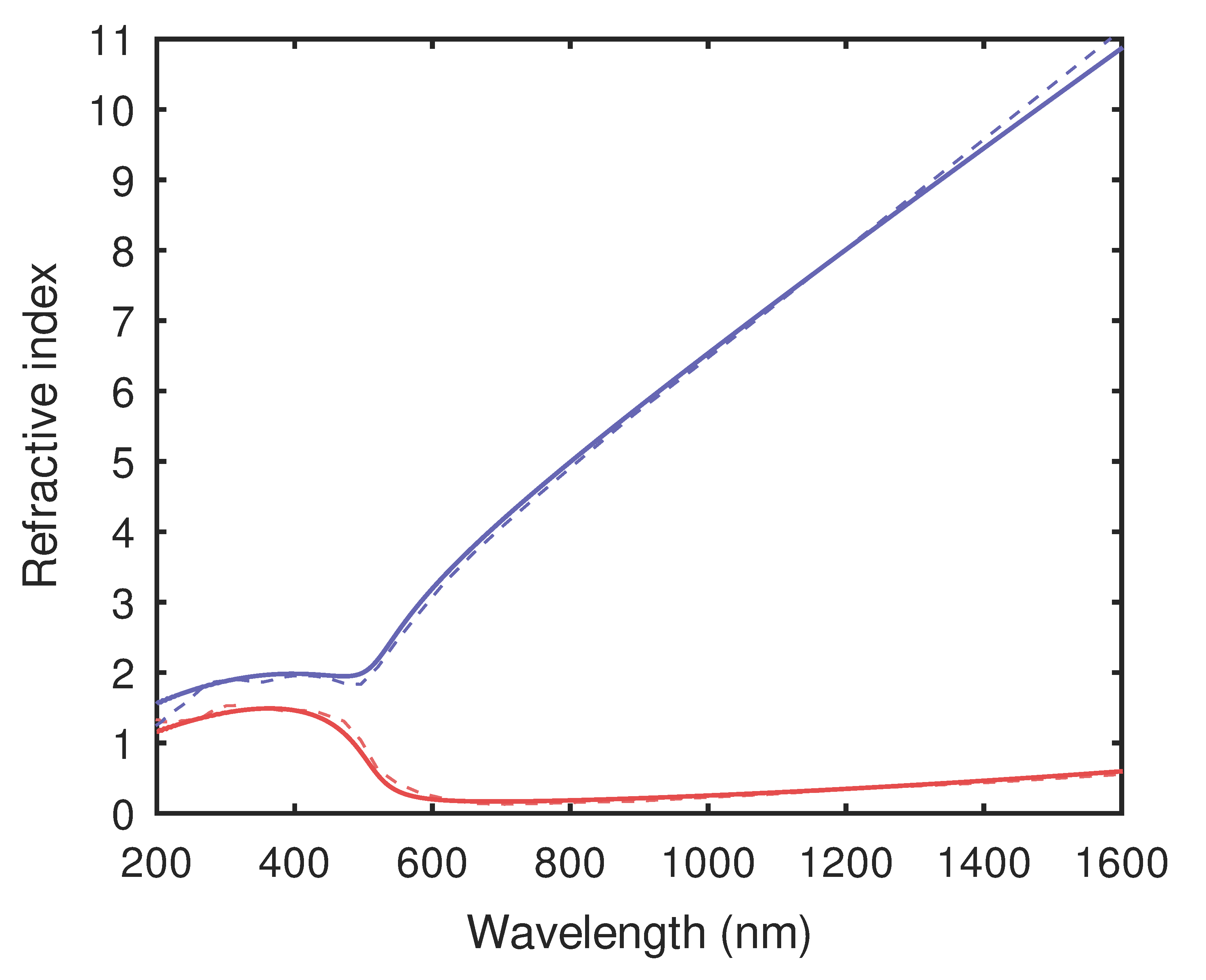
Figure 1: Johnson & Christy data (dashed lines) for the complex refractive index (real part: blue lines, imaginary part: red lines) of Gold in the range between 1600nm and 200nm as well as best fit (solid lines) of the parabolic two-band model via Eqs. (2), (3), and (5). The fit has been done for the range of 1937nm to 187nm. This is approximately the range considered in ref. [5].

The above gap frequency corresponds to an energy of 2.39 eV and, thus, is consistent with expectation. The fit shows very good agreement with the experimental data for wavelengths up to and including the violet part of the visible spectrum. For even shorter wavelengths, deviations between the experimental data and the fit become more pronounced. Obviously, the fit could be improved by considering transitions between, e.g., the 4d-band and the 6-sp band thereby extending the two-band model to a multi-band model. Nontheless, we would like to emphasize that the above results have been obtained with 6 fitting parameters while corresponding fits of comparable quality using Eq. (1) require at least 5 Lorentz terms and the usage of an $\epsilon_{\infty}$ instead of ‘1’ (see section 2.1), totalling at least 16 fitting parameters [5].

3 Time-domain modeling of interband transitions

As described above, in time-domain numerical schemes of Maxwell’s equations frequency-dependent permittivities are usually treated via ADEs. Unfortunately, while Eq. (3) is amenable to an ADE approach, Eq. (5) is not. And neither is its closed-form solution in terms of a sum of arc tangents. Therefore, in this section, we will develop an appropriate scheme for handling Eq. (5) via ADEs to any desired accuracy without introducing additional fitting parameters.

3.1 Discretization of the parabolic two-band model

The specific form of Eq. (5) suggests that we discretize the integral via a Gauss quadrature rule according to

$$\int_{a}^{b}{\rm d}x\,f(x) \approx\frac{b-a}{2}\,\sum_{i=1}^{N_{\rm G}}w_{i}\,f(u_{i}).$$ (7)

Here, $u_{i}=(a+b)/2+x_{i}(b-a)/2$ with $i=1,\dots,N_{\rm G}$ denote the Gauss quadrature nodes which are expressed in terms of the roots $x_{i}$ of the Legendre polynomial $P_{N_{\rm G}}(x)$ of order $N_{\rm G}$ within the interval $[-1,1]$ [25]. In addition, the weights $w_{i}$ are given $w_{i}=-2/((1-x_{i}^{2})(P_{N_{\rm G}}^{\prime}(x_{i})^{2})$ so that Eq. (7) integrates exactly polynomials of degree $2N_{\rm G}-1$ [25].
Upon applying the above Gauss quadrature to Eq. (5), we obtain

$$\chi_{\rm EP}(\omega) \approx\sum_{m=1}^{N_{\rm G}}\frac{a_{m}^{2}}{c_{m}^{2}-(\omega+i\gamma)^{2}},$$ (8)

$$a_{m} =\sqrt{\frac{Q\,s_{\rm U}\,s_{m}^{2}w_{m}}{c_{m}}},\quad c_{m}=\omega_{g}+s_{m}^{2},\quad s_{m}=\frac{s_{\rm U}}{2}\left(x_{m}+1\right).$$ (9)

With the above discretization (8) of the single particle contribution within the parabolic two-band model, Eq. (5), we end up with a set of effective Lorentz poles which can be included into time-domain simulations of Maxwell’s equations via ADEs. The number $N_{\rm G}$ of these Lorentz poles controls the level of accuracy with which we are approximating Eq. (5). However, contrary to the standard Drude-Lorentz approximations based on Eq. (1) or Lorentz-pole-only approximations [5], our approximation scheme, Eqs. (2), (3), and (8), does not introduce any additional fit parameters when increasing the number of Lorentz poles (or, equivalently, when increasing the accuracy of the approximation).

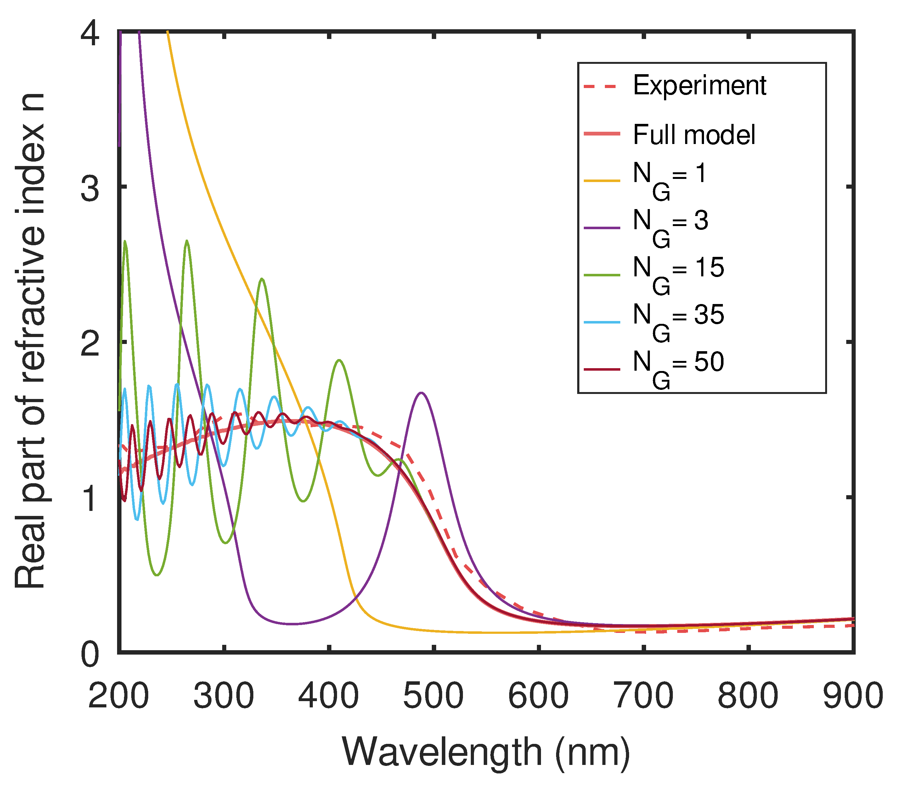
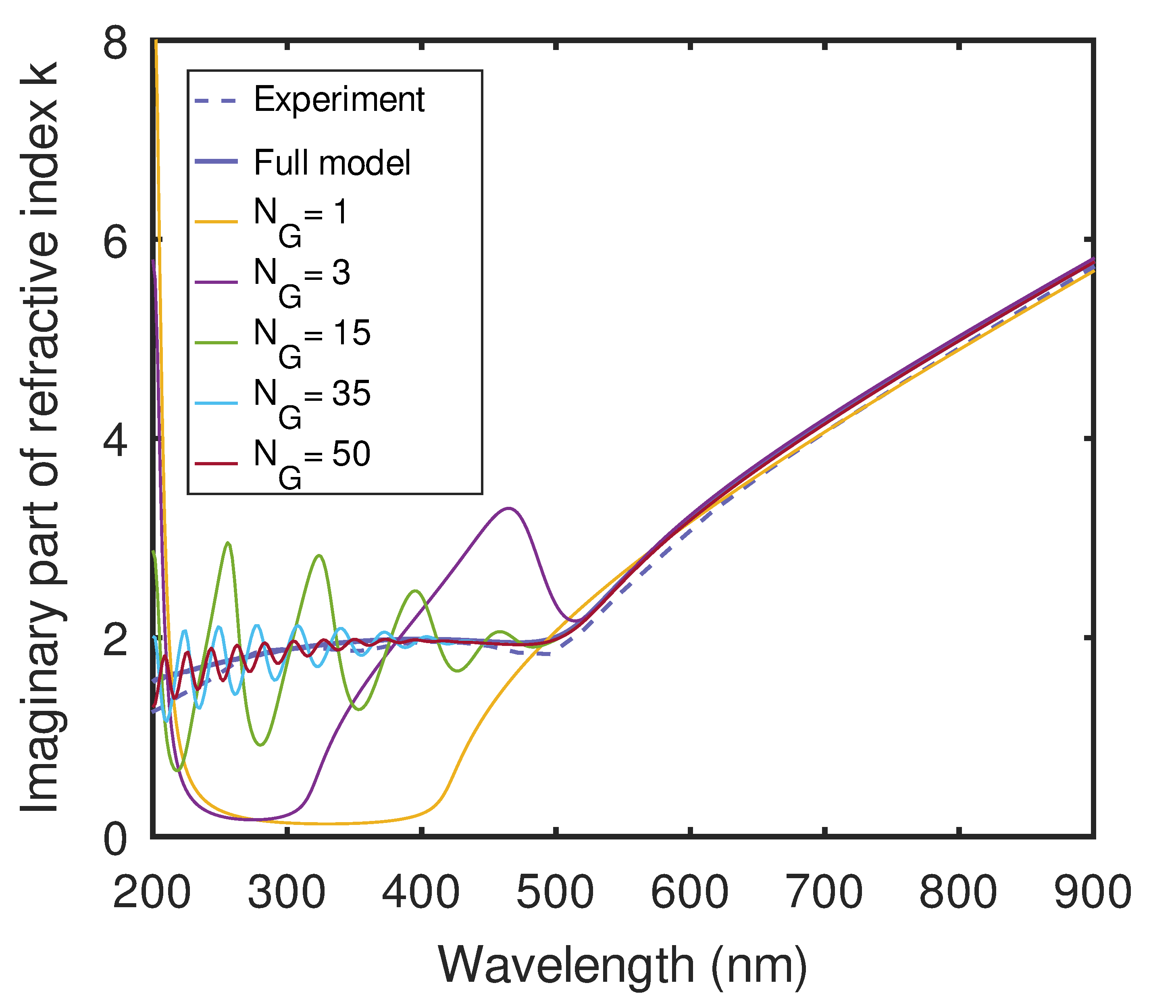
Figure 2: Complex refractive index of Gold for different Gauss quadratures of the parabolic two-band model in the range between 200nm and 900nm. Left panel: Real part of the refractive index. Right panel: Imaginary part of the refractive index. The free interband parameters $Q$, $\omega_{g}$, $\gamma$, and $s_{\rm U}$ have been determined by fitting Eqs. (2), (3), and (5) to the experimental data of Johnson & Christy (dashed lines). When the number $N_{\rm G}$ of Lorentz-poles (i.e., Gauss-quadrature points) increases, both, real and imaginary part, converge to the full model.

In Fig. 2, we depict details of the accuracy of our effective Lorentz-pole discretization for Gold. A single effective Lorentz pole works very well for wavelengths larger than about 600nm, an approximation based on three effective Lorentz poles works well down to about 550nm. For smaller wavelengths a considerably larger number of Lorentz poles is required for obtaining accurate results. In particular, by its very nature, the Lorentz pole approximation leads to unphysical peaks both, in the real and imaginary part of the complex refractive index which only become less pronounced when the number of effective Lorentz poles is increased. Therefore, considerable care must be exercised when designing Gold-based plasmonic elements for operation below 600nm. Nonetheless, we would like to point out that independent of how many effective Lorentz poles we use, we still have only the four fit parameters discussed above. Using only these four fit parameters, we have in hand a systematic way of improving the accuracy of our modeling of the dielectric properties of Gold via ‘simply’ increasing the number of effective Lorentz poles, thus allowing us to avoid unsubstantiated or unphysical designs and results.

3.2 Alternative Discretization of the parabolic two-band model

Based on the above considerations, we consider a variant of the above approach. For a given $N_{\rm G}$, we may regard Eqs. (2), (3), and (8) as a replacement of Eq. (1) with fixed Drude parameters $\omega_{p}$ and $\gamma_{\rm D}$ and a set of four fit parameters $Q$, $\omega_{g}$, $\gamma$, and $s_{\rm U}$. We then proceed to fit the resulting approximation to the experimental data. Note, that in this approach, for different values of $N_{\rm G}$, we obtain (slightly) different values for these four fit parameters. In Fig. 3 we depict the results of such a strategy for different numbers $N_{\rm G}$ of Lorentz poles. The corresponding values of the fit parameters are summarized in Tab. 1.

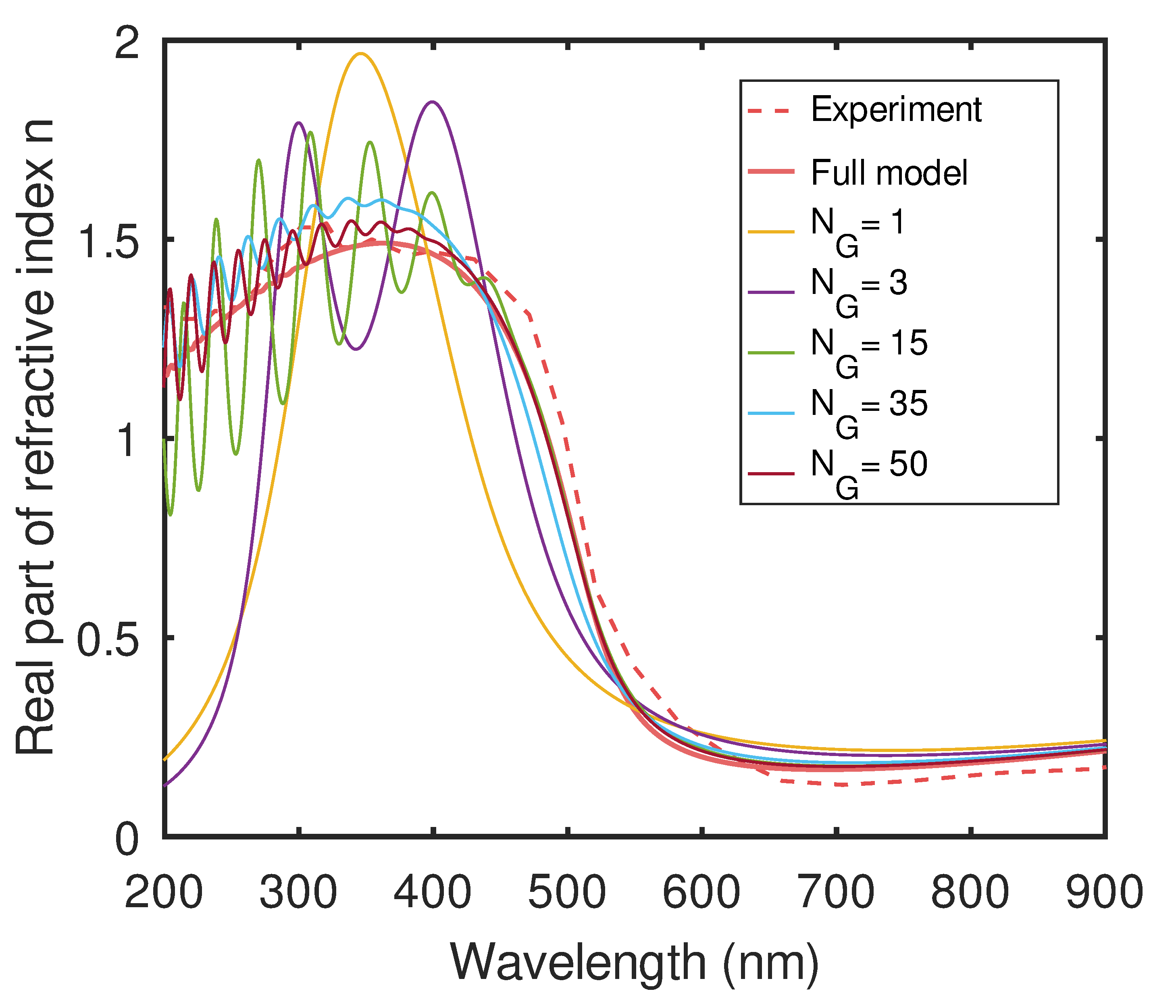
Figure 3: Complex refractive index of Gold for the alternative approach to Gauss quadrature approximations of the parabolic two-band model in the range between 200nm and 900nm. Left panel: Real part of the refractive index. Right panel: Imaginary part of the refractive index. Contrary to the results depicted in Fig. 2, in this approach IBT-integral Eq. (5) is first discretized with a Gauss quadrature scheme with $N_{\rm G}$ points (i.e. Lorentz poles) according to Eq. (8). Then, for this choice of $N_{\rm G}$, the free parameters $Q$, $\omega_{g}$, $\gamma$, and $s_{\rm U}$ are determined by fitting to the experimental data of Johnson & Christy (dashed lines). When the number $N_{\rm G}$ of Lorentz-poles (i.e., Gauss-quadrature points) increases, both, real and imaginary part, converge to the full model. An approximation with $N_{\rm G}=3$ Lorentz poles works well for wavelengths larger than 450nm and a significantly larger number of Lorentz poles is required for obtaining accurate results below 450nm. The values for the fit parameters are listed in Tab. 1.

$N_{\rm G}$	$Q$ [1/Hz3/2]	$\omega_{g}$ [Hz]	$\gamma$ [Hz]	$s_{\rm U}$ [Hz1/2]
1	1.48*1027	1.00*1015	5.72*1015	9.52*106
3	5.69*1024	5.79*1014	4.10*1015	5.49*107
15	3.16*1024	2.79*1014	3.67*1015	8.36*107
35	3.16*1024	3.62*1014	3.77*1015	1.18*108
50	2.83*1024	2.72*1014	3.65*1015	1.48*108

Table 1: Values of the fit parameters for the alternative discretization of the parabolic two-band model for Gold. These values lead to the results of the complex refractive index depicted in Fig. 3.

The results of Fig. 3 show that this approach leads to a further improvement of the approximation. The single effective Lorentz pole approximation now works well for wavelengths larger than 550nm, while the approximation based on three effective Lorentz poles works well down to about 450nm. For even smaller wavelengths, a significantly larger number of effective Lorentz poles is required for accurate results where the discretization converges to the results displayed in Fig. 1. However, compared with the original discretization discussed in Sec. 3.1, the unphysical peaks in the complex refractive index are less pronounced within this alternative discretization scheme of the IBT-integral, thus somewhat alleviating but certainly not eliminating the afore-discussed problem of unphysical peaks in the complex refractive index.

4 Conclusions

In summary, we have developed an efficient model for the linear dielectric response of simple metals with an emphasis on treating interband transitions and the model’s incorporation into time-domain Maxwell solver. We have illustrated this approach by way for arguably the most important plasmonic material, Gold.
Our model is based on the notion of separating the metal electron’s hydrodynamic (intraband) characteristics from the interband transitions by way of an appropriate canonical transformation. The resulting effective modeling of interband transitions leads to an excellent agreement with experimental data by fitting only four free parameters.
In addition, we have demonstrated two close connected approaches how this model can be efficiently discretized for time-domain Maxwell simulations via an arbitrary number of effective Lorentz poles, thereby providing a systematic way of improving the results without introducing additional fit parameters. With three effective Lorentz poles these models work well for wavelengths larger than about 450nm and significantly more effective Lorentz poles are required for accurate results below 450nm. In this latter wavelength range, peaks associated with the effective Lorentz poles may lead to unphysical results. Consequently, the aforementioned systematic way of improving the discretization (which reduces the amplitudes of the Lorentz peaks) together with the fact that in all instances only six parameters – two for the Drude permittivity and four parameters for the interband transitions – represents a useful tool for numerical computations. Furthermore, we should like to mention that our model naturally allows more advanced treatments of the hydrodynamic (intraband) contributions well beyond the Drude model. Specifically, the Drude permittivity may simply be replaced by any of its nonlocal extensions [17]. As a result, our model will be very useful for accurate modeling of plasmonic nanostructures in regimes where both nonlocal and interband transitions are important.

5 Backmatter

Funding German Research Foundation (DFG), Collaborative Research Center 1375 Nonlinear Optics down to Atomic Scales (NOA), (project number 398816777).

Acknowledgments The authors thank the Deutsche Forschungsgemeinschaft (DFG) for funding the project (project number 398816777) within the framework of the CRC 1375 NOA.

Disclosures The authors declare no conflicts of interest.

Data availability Data underlying the results presented in this paper are not publicly available at this time but may be obtained from the authors upon reasonable request.

References

- [1] “Spectroscopic Ellipsometry: Principles and Applications,” H. Fujiwara, (John Wiley & Sons, 2007).
- [2] “Classical Electrodynamics,” J. D. Jackson, (Wiley, 3rd Ed., 1998).
- [3] W. von Sellmeier, “Zur Erklärung der abnormen Farbenfolge im Spectrum einiger Substanzen,” \JournalTitleAnnalen der Physik 219, 272–282 (1871).
- [4] A. B. Djurisic, T. Fritz, and K. Leo, “Modelling the optical constants of organic thin films: impact of the choice of objective function,” \JournalTitleJournal of Optics A: Pure and Applied Optics 2, 458–464 (2000).
- [5] T. Gharbi, D. Barchiesi, S. Kessentini, and R. Maalej, “Fitting optical properties of metals by Drude-Lorentz and partial-fraction models in the [0.5;6] eV range,” \JournalTitleOptical Materials Express 10, 1129–1162 (2020).
- [6] P. B. Johnson and R. W. Christy, “Optical Constants of the Noble Metals,” \JournalTitlePhysical Review B 6, 4370–4379 (1972).
- [7] “Handbook of Optical Constants of Solids,” E. D. Palik, (Academic Press, 3rd Ed., 1998).
- [8] C. G. Darwin, “The Refractive Index of an Ionized Medium,” \JournalTitleProceedings of the Royal Society A 146, 17–45 (1934).
- [9] C. G. Darwin, “The refractive index of an ionized medium. II,” \JournalTitleProceedings of the Royal Society A 182, 152–166 (1943).
- [10] D. Bohm and D. Pines, “A Collective Description of Electron Interactions. I. Magnetic Interactions,” \JournalTitlePhysical Review 82, 625–634 (1951).
- [11] D. Pines and D. Bohm, “A Collective Description of Electron Interactions: II. Collective vs. Individual Particle Aspects of the Interactions,” \JournalTitlePhysical Review 85, 338–353 (1952).
- [12] D. Bohm and D. Pines, “A Collective Description of Electron Interactions: III. Coulomb Interactions in a Degenerate Electron Gas,” \JournalTitlePhysical Review 92, 609–625 (1953).
- [13] D. Pines, “A Collective Description of Electron Interactions: IV. Electron Interaction in Metals,” \JournalTitlePhysical Review 92, 626–636 (1951).
- [14] “Theory of Quantum Liquids,” D. Pines and P. Nozieres, (Perseus, 1999).
- [15] R. L. Olmon, B. Slovick, T. W. Johnson, D. Shelton, S-H. Oh, G. D. Boreman, and M. B. Raschke, “Optical dielectric function of gold,” \JournalTitlePhysical Review B 86, 235147/1–9 (2012).
- [16] C. Wolff, R. Rodriguez-Oliveros, and K. Busch “Simple magneto-optic transition metal models for time–domain simulations,” \JournalTitleOptics Express 21, 12022–12037 (2013).
- [17] N. A. Mortensen, “Mesoscopic electrodynamics at metal surfaces – From quantum-corrected hydrodynamics to microscopic surface-response formalism,” \JournalTitleNanophotonics 10, 2563–2616 (2021).
- [18] S. Raza, S. I. Bozhevolnyi, M. Wubs, and N. A. Mortensen, “Nonlocal optical response in metallic nanostructures,” \JournalTitleJournal of Physics: Condensed Matter 27, 183204/1–17 (2015).
- [19] G. Toscano, J. Straubel, A. Kwiatkowski, C. Rockstuhl, F. Evers, H. Xu, N. A. Mortensen, and M. Wubs, “Resonance shifts and spill-out effects in self-consistent hydrodynamic nanoplasmonics,” \JournalTitleNature Communications 6, 7132/1–11 (2015).
- [20] C. Ciracì and F. Della Sala, “Quantum hydrodynamic theory for plasmonics: Impact of the electron density tail,” \JournalTitlePhysical Review B 93, 205405/1–14 (2016).
- [21] M. Moeferdt, T. Kiel, T. Sproll, F. Intravaia, and K. Busch, “Plasmonic modes in nanowire dimers: A study based on the hydrodynamic Drude model including nonlocal and nonlinear effects,” \JournalTitlePhysical Review B 97, 075431/1–10 (2018).
- [22] D. Reiche, K. Busch and F. Intavaia, “Quantum thermodynamics of overdamped modes in local and spatially dispersive materials,” \JournalTitlePhysical Review A 101, 012506/1–22 (2020).
- [23] G. M. Wysin, V. Chikan, N. Yang, and R. K. Dani, “Effects of interband transitions on Faraday rotation in metallic nanoparticles,” \JournalTitleJournal of Physics: Condensed Matter 25, 325302/1–16 (2013).
- [24] L. Le Thi Ngoc, J. Wiedemair, A. van den Berg, and E. T. Carlen, “Plasmon-modulated photoluminescence from gold nanostructures and its dependence on plasmon resonance, excitation energy, and band structure,” \JournalTitleOptics Express 23, 5547–5564 (2015).
- [25] “Numerical Recipies in Fortran 77,” W. H. Press, S. A. Teukolsky, W. T. Vetterling, and B. P. Flannery, (Cambridge University Press, 1986).
- [26] C. Varin, G. Bart, T. Fennel, and T. Brabec, “Nonlinear Lorentz model for the description of nonlinear optical dispersion in nanophotonics simulations,” \JournalTitleOptical Materials Express 9, 771–778 (2019).