CHAOS VII: A Large-Scale Direct Abundance Study in M33

Abstract

The dispersion in chemical abundances provides a very strong constraint on the processes that drive the chemical enrichment of galaxies. Due to its proximity, the spiral galaxy M33 has been the focus of numerous chemical abundance surveys to study the chemical enrichment and dispersion in abundances over large spatial scales. The CHemical Abundances Of Spirals (CHAOS) project has observed $\sim$100 H II regions in M33 with the Large Binocular Telescope (LBT), producing the largest homogeneous sample of electron temperatures (T_e) and direct abundances in this galaxy. Our LBT observations produce a robust oxygen abundance gradient of $-$0.037 $\pm$ 0.007 dex/kpc and indicate a relatively small (0.043 $\pm$ 0.015 dex) intrinsic dispersion in oxygen abundance relative to this gradient. The dispersions in N/H and N/O are similarly small and the abundances of Ne, S, Cl, and Ar relative to O are consistent with the solar ratio as expected for $\alpha$-process or $\alpha$-process-dependent elements. Taken together, the ISM in M33 is chemically well-mixed and homogeneously enriched from inside-out with no evidence of significant abundance variations at a given radius in the galaxy. Our results are compared to those of the numerous studies in the literature, and we discuss possible contaminating sources that can inflate abundance dispersion measurements. Importantly, if abundances are derived from a single T_e measurement and T_e-T_e relationships are relied on for inferring the temperature in the unmeasured ionization zone, this can lead to systematic biases which increase the measured dispersion up to 0.11 dex.

1 Introduction

The abundance of heavy elements in the Interstellar Medium (ISM) is entwined with the physical processes at work in a galaxy. High-mass stars forge these elements via stellar nucleosynthesis and release them into the gas via supernovae and mass-loss events. Galactic mixing processes distribute the metal-enriched gas through the ISM, while infall acts to dilute the ISM with pristine, metal-poor gas. As such, the distribution of gas-phase chemical abundances grants insight into star formation, galactic mixing mechanisms, and the overall chemical evolution of the galaxy. Observations of the ISM in spiral galaxies typically show a negative metallicity gradient with some scatter. That scatter, the dispersion about the abundance gradient, is a potentially powerful diagnostic of galaxy evolution. A large dispersion indicates that enrichment processes prevail over mixing processes. For example, if chemical enrichment is a local process, i.e., massive stars in clusters pollute their immediate environs, then large departures from the mean are possible as star formation regions at different positions in the spiral galaxy evolve independently. On the other hand, if chemical enrichment is more of a global process, i.e., supernovae expel their newly produced heavy elements into the hot phase of the galaxy where it mixes and dilutes before cooling, then the whole galaxy experiences chemical evolution in a more homogeneous manner.

High precision measurements of the chemical abundances in a large sample of star forming regions in a individual galaxy are necessary to accurately measure the dispersion about the mean metallicity gradient. Fortunately, optical emission from regions of ionized gas, or H II regions, contains a multitude of emission lines from the ions present in the gas. Despite the relatively low abundance of metal ions compared to H⁺, emission from the forbidden transitions of O⁺, O⁺⁺, N⁺, and others are comparable in strength to the Balmer series. Intensity ratios of various collisionally-excited lines (CELs) from the same ion but originating from different energy levels can be exponentially sensitive to the physical conditions within the region, such as the electron gas temperature (T_e) or density (n_e). Provided these physical conditions, the ionic abundances of many ions can be directly calculated via the intensity of the observed CELs and the emissivities of the transitions as a function of T_e and n_e.

The direct abundance method (Dinerstein, 1990) is often viewed as the gold standard when it comes to abundance techniques. Firstly, the emission lines necessary to measure the electron temperature and calculate ionic abundances are all within the optical, enabling ground-based observations. The optical band also contains the emission from the dominant ionization states of oxygen, which permits an accurate measure of the abundance of oxygen without the corrections for unobserved ionization states. Secondly, this abundance technique utilizes the derived physical properties within the nebula instead of relying on indicators that may not be calibrated or well-constrained at all physical conditions. Finally, this technique can be applied to multiple ionic species to obtain T_e from numerous ionization zones within a region, thereby uncovering the temperature structure within the ionized gas.

While the direct method does have shortcomings, most notably the potential for an upward bias in temperature in the presence of temperature inhomogeneities (Peimbert, 1967), presently it is the only method which allows for a robust measurement of the metallicity dispersion. The uncertainties on strong line method metallicities of individual H II regions are too large to accurately measure the dispersion. Fine structure and recombination line measurements cannot provide the large sampling necessary.

Thus, direct abundances of large, homogeneous samples are required to better understand the chemical evolution of the ISM. Local spiral galaxies present the best opportunity to study gas-phase abundances in a large quantity of H II regions with sampling on small spatial scales. A quintessential example of such a spiral galaxy is M33; the third largest member of the Local Group, M33 is very close (adopted distance of 0.86 Mpc from Savino et al., 2022), relatively face-on (inclination $\sim$55$\arcdeg$), and hosts a number of bright H II regions across the disk of the galaxy. Given its angular size and proximity, M33 has been the focus of many pioneering chemical abundances studies (Smith, 1975; Kwitter & Aller, 1981; Diaz & Tosi, 1984; Vilchez et al., 1988). Modern, large-scale optical surveys include H II region chemical abundances from the direct (Crockett et al., 2006; Magrini et al., 2007; Rosolowsky & Simon, 2008; Magrini et al., 2010; Bresolin, 2011; Toribio San Cipriano et al., 2016; Lin et al., 2017; Alexeeva & Zhao, 2022) and strong-line methods (Lin et al., 2017; Alexeeva & Zhao, 2022). Additionally, there are existing recombination line (Esteban et al., 2009; Toribio San Cipriano et al., 2016) and stellar abundances (U et al., 2009) in M33.

The full literature sample is one of the largest H II region compilations in a nearby spiral galaxy, consisting of a large range in physical and ionization conditions in the ISM. However, the sample’s coverage and scope is offset by its inhomogeneity. To start, a variety of detectors, all of which have varying wavelength coverage and spectral resolution, are used to obtain the optical spectra. Furthermore, the H II regions selected within each sample are optimized for different studies of the ISM. For example, samples targeting many H II regions across the disk of the galaxy are beneficial for an accurate measure of the abundance gradient and dispersion about it (e.g., Rosolowsky & Simon, 2008). Other samples (e.g., Esteban et al., 2009; Toribio San Cipriano et al., 2016) focus on relatively few, bright regions for the most reliable direct and recombination line (RL) abundances for insight into the Abundance Discrepancy, or the consistent trend that RL abundances are significantly larger (around a factor of 2 in H II regions) than CEL abundances as measured in the same object (Peimbert & Peimbert, 2005; García-Rojas & Esteban, 2007; Esteban et al., 2009; García-Rojas et al., 2013). Many studies in the literature were observed at relatively low spectroscopic resolution ($\geq$ 5 Å) which is insufficient for isolating key emission lines from other emission lines or atmospheric features. Finally, each study selects its own atomic data, reddening determination method, electron temperature relations, etc., based on the available spectroscopic data. As such, the literature temperatures and/or abundances in M33 cannot necessarily be compared on a simple one-to-one basis.

To better understand the chemical evolution of this important galaxy, and to complement previous chemical abundance studies, the CHemical Abundances Of Spirals (CHAOS) project (Berg et al., 2015) has observed a large population of H II regions in M33. To date, CHAOS has accumulated 200+ high-resolution H II region spectra in nearby, face-on spiral galaxies. With this database, CHAOS has measured statistically-significant direct oxygen abundance gradients in five galaxies, found evidence of universal secondary N/O gradients in local spirals, measured C II recombination line abundances of bright regions, and developed robust empirical T_e-T_e relations and a new method of application for these relations (Berg et al., 2015; Croxall et al., 2015, 2016; Berg et al., 2020; Skillman et al., 2020; Rogers et al., 2021). The H II regions of M33 with auroral line detections increases the database by almost 33%, but the real advantage is its wealth of direct abundance data and homogeneity.

This study is organized as follows: In §2 we introduce the observations and reduction of the CHAOS M33 data, and present the literature samples we compare to. The parameters used for direct abundances, including T_e and Ionization Correction Factors (ICFs), are discussed in §3. The oxygen abundances, gradient, and dispersion in M33 as well as the abundance of other heavy elements (N, Ne, S, Cl, Ar) are reported in §4. We compare our results to the literature, discuss possible sources of T_e contamination (some unique to M33), and contextualize the abundance dispersion observed in local spiral galaxies in §5. We summarize our conclusions in §6.

2 Observations and Reduction

Table 1: M33 Global Properties

Property	Adopted Value	Reference
R.A.	01h33m50.6s	1
Decl.	+30∘39m29.9s	1
Inclination	55.08∘	1
Position Angle	201.12∘	1
Distance	859${}^{+24}_{-23}$ kpc	2
log(M⋆/M⊙)	9.68	3
Re	555″, 2.31 kpc	4
Redshift	$-$0.000597	1

Note. — Units of right ascension are hours, minutes, and seconds, and units of declination are degrees, arcminutes, and arcseconds. References: [1] Koch et al. (2018) [2] Savino et al. (2022) [3] Corbelli et al. (2014) [4] Leroy et al. (2019, 2021)

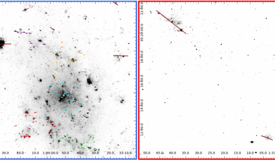
Figure 1: A continuum-subtracted H$\alpha$ image of M33 from Massey et al. (2006) retrieved from NASA/IPAC Extragalactic Database (2019) with the CHAOS slits superimposed on the targeted regions. The R.A. and Decl. are reported on the vertical and horizontal axes, respectively. Left: H$\alpha$ image of the center of M33. This image encompasses the five MOS fields (Red, Orange, Green, Cyan, and Purple slits) and four longslit pointings (Brown slits). Right: H$\alpha$ image focused on the far southern portion of M33. Two longslit pointings are provided as the Brown slits.

2.1 CHAOS Observations of M33

The CHAOS project utilizes the Multi-Object Double Spectrographs (MODS, Pogge et al., 2010) on the Large Binocular Telescope (LBT, Hill, 2010) to obtain the optical spectra of H II regions in nearby spiral galaxies. The MODS blue channel has a wavelength coverage of 3200–5700 Å and R$\sim$1850 for the G400L (400 lines mm^-1) grating; the red channel has a wavelength range of 5500–10000 Å and R$\sim$2300 for the G670L (250 lines mm^-1) grating. In combination, these spectrographs cover the full optical band and extend into the NIR at sufficient resolution for direct abundance analysis. Multi-object slit (MOS) masks can observe $\sim$20 objects in one 6′$\times$6′ field of view, while longslits can target objects that are too extended (in galactocentric radius or in emission) for the MOS masks. The versatility, sensitivity, resolution, and wavelength coverage of MODS permits a thorough examination of the direct abundances in M33 and other nearby spiral galaxies.

For M33’s parameters, we adopt the disc parameters of center, position angle, and inclination that Koch et al. (2018) derive from a fit to the velocity field derived from combined VLA and GBT H I 21 cm observations. These properties are provided in Table 1. Note that the single values of position angle and inclination do not account for the outer warp (cf., Corbelli et al., 2014) but that feature appears beyond $\sim$ 8 kpc, and is not relevant for our H II region sample. There are many distances to M33 in the literature to choose from (see discussion in de Grijs et al., 2017; Lee et al., 2022). We adopt the distance modulus of 24.67$\pm$0.06 (corresponding to 859${}^{+24}_{-23}$ kpc) based on HST observations of RR Lyrae (Savino et al., 2022) anchored to the GAIA eDR3 reference frame (Nagarajan et al., 2021), which is consistent with the values favored by de Grijs et al. (2017) and Lee et al. (2022). The effective radius of M33, R_e, is determined from the z0MGS WISE 3.4$\mu$m maps (Leroy et al., 2019) with the same fitting method as described in Leroy et al. (2021) and which has been utilized in previous CHAOS studies (e.g., Berg et al., 2020).

Given its proximity and wealth of H II regions, CHAOS observed five MOS fields in M33 with an additional six longslit pointings. All MOS observations and the majority of the longslit observations took place between 2015 October 11 and 15; the remaining longslit pointings were taken 2015 December. Each MOS field was observed in six 1200 second exposures, while longslit pointings were observed for three 1200 second exposures. The standard star G191-B2B was observed on multiple nights for flux calibration. The width of each slit in the MOS masks was 1$\farcs$0 and the length ranged from 6$\farcs$0–30$\farcs$0; the longslits are a combination of five 60$\farcs$0$\times$1$\farcs$0 slits. The airmasses of the observations varied depending on the time of observation, and the position angle was chosen to be equal to the parallactic angle halfway through a pointing to minimize flux losses due to differential atmospheric refraction (Filippenko, 1982). In total, 99 slits target ionized regions based on their surface brightness, location, and overlap with previous direct abundance studies. Figure 1 provides a continuum-subtracted H$\alpha$ image of M33 along with the MOS and longslit locations of the CHAOS observations. Table 2 provides the name, location, and radius for each H II region observed in M33. Consistent with previous works, we report the name of the H II region as the offset in R.A. and Decl. of the center of the extraction profile relative to the center of the galaxy (provided in Table 1).

2.2 Data Reduction and Processing

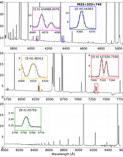
Figure 2: Example MODS spectrum of M33+333+745. Temperature-sensitive auroral lines and their model fits (Gaussian plus STARLIGHT continuum) are provided in the subplots. All five commonly-employed auroral lines are detected at high S/N. While the spectrum has been corrected for the systemic velocity of M33, the rotational velocity of this extended region has shifted the lines blueward of their theoretical wavelengths (vertical dotted blue lines).

Aspects of the MODS data reduction pipeline are detailed in previous works (Berg et al., 2015; Rogers et al., 2021). As such, we only provide a brief summary of the steps taken. The modsCCDRed Python programs (Pogge, 2019) are used to bias subtract and flat field the raw images before combination. Standard star and science images are median combined, then are input into the modsIDL pipeline (Croxall & Pogge, 2019). Standard stars, which are observed on each night of science observation, are processed and used for flux calibration (Bohlin et al., 2014). Sky subtraction and region extraction are performed on each slit while allowing for multiple sky areas or H II regions to be extracted within the same slit. Each MOS mask has at least two slits cut away from any prominent ionized gas and which can be used if local sky subtraction is not possible in one of the MOS slits. Finally, the blue and red spectra are re-sampled and combined at 5700 Å. As an example of the sensitivity and wavelength coverage of MODS, Figure 2 plots the high-S/N spectrum of the H II region M33+333+745. This region has clearly-detected T_e-sensitive auroral lines, Balmer and Paschen sequences, and faint emission lines from other metal ions such as C II and [Cl III].

The underlying stellar continuum within an H II region is fit using the STARLIGHTv04 spectral synthesis code (Cid Fernandes et al., 2005) with the stellar population models of Bruzual & Charlot (2003). We mask out strong nebular lines and the area near the dichroic cross-over when fitting the stellar continuum, and we allow for a linear, nebular continuum component in the total fit. The net continuum is subtracted from the spectrum, and the emission lines are fit with Gaussian profiles. The full spectrum is broken into ten wavelength bands in which all Gaussian profiles have the same full width at half maximum (FWHM) and global velocity shift. Line multiplets that are blended at MODS’s resolution, such as [O II]$\lambda\lambda$3726,3729, are fit using Gaussians with fixed wavelength separation and FWHM.

Table 2: M33 LBT/MODS Observations

H II	R.A.	Dec.	Rg	Rg/Re	Literature	H II	R.A.	Dec.	Rg	Rg/Re	Literature
Region	(J2000)	(J2000)	(kpc)		Obs.	Region	(J2000)	(J2000)	(kpc)		Obs.
M33$-$2+25	1:33:50.4	30:39:55.37	0.13	0.05		M33$-$224$-$437	1:33:33.2	30:32:13.23	2.07	0.89
M33+23$-$9	1:33:52.4	30:39:20.98	0.18	0.08		M33+253$-$141	1:34:10.1	30:37:09.18	2.09	0.90
M33$-$23+16	1:33:48.8	30:39:45.97	0.20	0.09		M33+19+466	1:33:52.1	30:47:15.83	2.14	0.93
M33$-$28+6	1:33:48.4	30:39:35.66	0.21	0.09	R08,B11,T16,L17	M33+263+423	1:34:10.9	30:46:32.85	2.15	0.93
M33$-$36$-$52	1:33:47.8	30:38:37.55	0.28	0.12	R08,B11,T16	M33+209+473	1:34:06.8	30:47:22.42	2.16	0.93
M33+2+111	1:33:50.7	30:41:20.96	0.52	0.22		M33+285+399	1:34:12.6	30:46:08.4	2.17	0.94
M33$-$6$-$120	1:33:50.1	30:37:30.09	0.55	0.24	C06,R08,B11	M33+221+476	1:34:07.7	30:47:25.68	2.20	0.95
M33+78+91	1:33:56.6	30:41:00.69	0.55	0.24		M33$-$263$-$461	1:33:30.2	30:31:48.66	2.26	0.98	L17
M33$-$89$-$21	1:33:43.7	30:39:08.91	0.59	0.25		M33$-$267$-$462	1:33:29.9	30:31:47.76	2.27	0.98
M33$-$42$-$138	1:33:47.3	30:37:12.06	0.60	0.26		M33$-$128+386	1:33:40.6	30:45:55.93	2.29	0.99
M33+108+25	1:33:58.9	30:39:55.33	0.71	0.31		M33$-$143+371	1:33:39.5	30:45:40.56	2.30	0.99	A22
M33$-$66$-$161	1:33:45.5	30:36:48.59	0.73	0.31	R08,B11	M33+285+456	1:34:12.6	30:47:05.86	2.32	1.00
M33$-$114$-$123	1:33:41.7	30:37:26.61	0.79	0.34		M33+267$-$191	1:34:11.2	30:36:19.22	2.34	1.01
M33+89+165	1:33:57.5	30:42:14.43	0.79	0.34		M33+121$-$405	1:33:60.0	30:32:44.53	2.34	1.01	B11,L17
M33$-$88$-$166	1:33:43.8	30:36:43.67	0.79	0.34		M33+300+471	1:34:13.8	30:47:20.71	2.42	1.05
M33+125+78	1:34:00.2	30:40:47.65	0.81	0.35	R08	M33+266$-$221	1:34:11.2	30:35:48.77	2.43	1.05
M33$-$89+89	1:33:43.7	30:40:58.55	0.86	0.37	B11	M33+299$-$164	1:34:13.7	30:36:45.89	2.46	1.07
M33$-$144$-$78	1:33:39.4	30:38:12.2	0.93	0.40		M33+208+567	1:34:06.7	30:48:56.99	2.52	1.09
M33$-$150$-$79	1:33:39.0	30:38:10.55	0.97	0.42		M33+94+574	1:33:57.8	30:49:04.34	2.53	1.09	C06
M33+70+228	1:33:56.0	30:43:17.42	1.00	0.43		M33+107+581	1:33:58.9	30:49:11.22	2.55	1.10	A22
M33+29+261	1:33:52.8	30:43:51.29	1.17	0.50		M33+322$-$139	1:34:15.5	30:37:10.79	2.55	1.10	R08,T16,L17,A22
M33+135+264	1:34:01.0	30:43:53.91	1.25	0.54	L17	M33+119+592	1:33:59.8	30:49:21.71	2.59	1.12
M33+146+266	1:34:01.9	30:43:56.26	1.29	0.56		M33+299+541	1:34:13.7	30:48:30.9	2.62	1.13	A22
M33+143+328	1:34:01.7	30:44:57.46	1.49	0.65		M33+334$-$135	1:34:16.5	30:37:14.7	2.62	1.13	L17
M33$-$24$-$333	1:33:48.7	30:33:56.89	1.51	0.65		M33+328+543	1:34:16.0	30:48:33.03	2.72	1.18
M33+113$-$224	1:33:59.3	30:35:46.33	1.52	0.66	B11	M33+306$-$276	1:34:14.2	30:34:53.62	2.87	1.24
M33+69+352	1:33:55.9	30:45:21.87	1.54	0.67		M33+369+545	1:34:19.2	30:48:34.82	2.88	1.25
M33+88$-$258	1:33:57.4	30:35:11.76	1.54	0.67		M33+380+578	1:34:20.0	30:49:07.66	3.01	1.30
M33+62+354	1:33:55.4	30:45:23.73	1.55	0.67		M33+400+552	1:34:21.6	30:48:41.86	3.02	1.31
M33$-$36+312	1:33:47.8	30:44:42.04	1.57	0.68		M33+405+554	1:34:22.0	30:48:43.29	3.05	1.32
M33$-$2$-$340	1:33:50.4	30:33:49.51	1.59	0.69		M33+298$-$344	1:34:13.7	30:33:45.39	3.06	1.32	R08,L17
M33$-$65+302	1:33:45.5	30:44:31.99	1.64	0.71		M33+421+560	1:34:23.2	30:48:50.12	3.13	1.35
M33$-$108$-$389	1:33:42.2	30:33:01.36	1.70	0.73		M33+313$-$342	1:34:14.8	30:33:48.01	3.14	1.36	L17
M33+14$-$355	1:33:51.7	30:33:34.98	1.70	0.74		M33+325$-$329	1:34:15.7	30:34:00.6	3.17	1.37
M33+33+382	1:33:53.1	30:45:51.7	1.72	0.74		M33+330$-$345	1:34:16.1	30:33:44.81	3.25	1.41
M33$-$35$-$385	1:33:47.8	30:33:04.79	1.73	0.75	B11	M33+345$-$344	1:34:17.3	30:33:45.44	3.34	1.45	R08
M33$-$78+311	1:33:44.5	30:44:41.0	1.73	0.75		M33+333+745	1:34:16.5	30:51:54.32	3.41	1.47	C06,L17
M33$-$224$-$346	1:33:33.2	30:33:43.31	1.79	0.77		M33+417$-$254	1:34:22.9	30:35:16.08	3.51	1.52
M33+116$-$286	1:33:59.5	30:34:43.51	1.80	0.78	A22	M33+371$-$348	1:34:19.3	30:33:41.27	3.52	1.52	R08
M33$-$99+311	1:33:42.9	30:44:40.53	1.83	0.79	A22	M33+388$-$320	1:34:20.6	30:34:09.93	3.53	1.53
M33$-$148$-$412	1:33:39.1	30:32:37.49	1.83	0.79		M33+541+448	1:34:32.6	30:46:57.31	3.57	1.55	L17
M33$-$196$-$396	1:33:35.4	30:32:53.73	1.86	0.80		M33+553+448	1:34:33.5	30:46:57.07	3.64	1.57
M33+122$-$294	1:34:00.0	30:34:36.04	1.87	0.81		M33$-$464+348	1:33:14.5	30:45:17.71	4.12	1.78	L17
M33+26+421	1:33:52.6	30:46:30.62	1.91	0.83		M33$-$507+346	1:33:11.3	30:45:15.59	4.38	1.90	C06,T16,A22
M33+46$-$380	1:33:54.1	30:33:09.67	1.92	0.83	R08,B11	M33$-$72$-$1072	1:33:45.0	30:21:38.08	4.86	2.10	R08,L17,A22
M33+126$-$313	1:34:00.3	30:34:17.13	1.97	0.85	R08,B11,T16	M33$-$181$-$1156	1:33:36.6	30:20:13.48	5.09	2.20	R08,L17
M33$-$77$-$449	1:33:44.6	30:32:01.2	1.97	0.85	B11,A22	M33$-$438+800	1:33:16.6	30:52:49.7	5.63	2.44	L17,A22
M33$-$168$-$448	1:33:37.6	30:32:02.18	1.99	0.86		M33$-$442+797	1:33:16.2	30:52:46.13	5.64	2.44	A22
M33+175+446	1:34:04.1	30:46:55.4	1.99	0.86		M33$-$610$-$1690	1:33:03.5	30:11:19.06	7.49	3.24	C06,L17
M33$-$211$-$438	1:33:34.2	30:32:12.21	2.04	0.88	R08,L17

Note. — Compilation of H II regions CHAOS observed in M33. Columns 1 and 7: H II region ID given by the R.A. and Decl. offset relative to the center of M33. Columns 2 and 8: R.A. of the H II region in hours, minutes, and seconds. Columns 3 and 9: Decl. of the H II region in degrees, arcminutes, and arcseconds. Columns 4 and 10: H II region distance from the center of M33 in kpc. Columns 5 and 11: H II region distance from the center of M33 normalized to the effective radius of the galaxy. Columns 6 and 12: Literature studies that have observed the H II region, see text for shorthand citations (Section 2.3).

The direct temperature method is exponentially sensitive to the auroral-to-nebular line ratio, requiring utmost care when fitting these lines. The Gaussian fit to each line is checked against a fit of the profile using the IRAF splot routine; the flux of the emission line and RMS noise in the continuum are updated to the splot values only when the there is significant disagreement with the modsIDL fitting program. The uncertainty on the emission line flux, adapted from Berg et al. (2013) and reported in Rogers et al. (2021), is a combination of RMS noise in the continuum around the line profile and a 2% uncertainty associated with the standard star flux calibration (Oke, 1990).

The exception to the above fitting routine is for the Balmer lines, which are necessary to measure the line-of-sight reddening for each region. The reddening method that we employ is described in Rogers et al. (2021) and is a modified version of the technique detailed in Olive & Skillman (2001) with an MCMC component expanded upon by Aver et al. (2021). In short, we fit a linear function to the continuum across the stellar absorption well, and then fit a Gaussian profile to the Balmer line above the well. Theoretical Balmer line ratios are calculated for n_e = 10² cm^-3 and T_e = 10⁴ K from the tables of Storey & Hummer (1995). We then determine the combination of $c(H\beta)$ and the equivalent width of the stellar Balmer absorption features, $a_{H}$, that produces agreement between the measured and theoretical H$\alpha$/H$\beta$, H$\gamma$/H$\beta$, and H$\delta$/H$\beta$ ratios. The spectrum is reddening corrected using the best-fit $c(H\beta)$ and the reddening law from Cardelli et al. (1989) assuming R_V = 3.1. The electron temperatures are calculated from the resulting line intensities, and new theoretical Balmer line ratios are generated for the determined T_e. The process is iterated until convergence (change in T_e $<$ 20 K).

In Table A.1, we provide the emission line detections for each H II region. Only emission lines with S/N $>$ 3 are considered detected and, subsequently, used for temperature/abundance analysis. In addition to the auroral line detections, we also indicate the detection of other significant emission lines (Columns 8-11) and the presence of Wolf-Rayet features (Column 12). Table A.2 in the Appendix provides the emission line intensities, $c(H\beta)$, and $a_{H}$ for each region. We report the combined flux of [O II]$\lambda\lambda$3726,3729 as a single line, [O II]$\lambda$3727. We exclude the object M33$-$224$-$346 from the tables in the Appendix and from the following analysis because it is coincident with the Luminous Blue Variable (LBV) M33C-7256 (Massey et al., 2007; Humphreys et al., 2014). The spectrum of this object is characterized by intense Balmer, Fe II, and O I recombination lines while the [O II] and [O III] strong lines are extremely faint. The lack of [O II] and [O III] strong lines would indicate that the bulk of the emission is coming from the LBV and, therefore, the object should not be included in the following H II region abundance analysis.

Table 3: M33 Literature Direct Abundance Studies

Reference	$\lambda$ Coverage (Å)	Resolution	# H II Regions	Te-Sensitive Lines	Te-Te
			with Direct O/H		Relations
Crockett et al. (2006) (C06)	3600–5100	$\sim$2 Å	6	[O III]	[1]
Rosolowsky & Simon (2008) (R08)	3600–5400	$\sim$5 Å	61	[O III]	[1]
Bresolin (2011) (B11)	3500–5100	$\sim$5.5 Å	8	[O III]	[1]
Toribio San Cipriano et al. (2016) (T16)	3600–7600	R$\approx$2,500	11	[O III], [N II], [O II], [S II]	[2]
Lin et al. (2017) (L17)	3650–9200	$\sim$6.2 Å	38	[O III], [N II]	[1]
Alexeeva & Zhao (2022) (A22)	3700–9099	R$\approx$1,800	27	[O III], [N II], [O II]	None
This Study	3200–10000	R$\approx$2,000	65	[O III], [N II], [S III], [O II], [S II]	§3.1

Note. — The compilation of literature abundance studies which obtain T_e measurements in the H II  regions of M33. We focus on studies with many H II  regions from which abundance gradients can be measured. The columns provide the following information: reference to the study; the wavelength coverage of the detector used (in Å); the quoted resolution of the spectra; the reported number of regions with at least one T_e-sensitive auroral line detected; the T_e-sensitive lines detected in M33; and the T_e-T_e relations applied. The T_e-T_e relations are: [1] Campbell et al. (1986); Garnett (1992); [2] N/A unless missing [O III]$\lambda$4363, in which case use empirical relation from Esteban et al. (2009).

2.3 Ancillary Data

Table 3 compiles previous literature studies that obtain direct abundances in the H II regions of M33. While there are many prior abundance studies in M33 (including strong-line and recombination line abundances), we focus on this sample given the wealth of direct abundances and the coverage/overlap of the H II regions. No two samples in Table 3 are directly comparable: each has a different number of regions with T_e measurements, wavelength coverage, spectral resolution, and auroral lines used.

2.3.1 Crockett et al. (2006)

While early direct abundance studies of local galaxies included the bright H II regions in M33 (see Introduction), Crockett et al. (2006, hereafter C06) is the earliest study with a significant number of direct abundances in M33. C06 observed 13 H II regions with the Mayall Telescope at Kitt Peak National Observatory and obtained optical spectra in the wavelength range 3600–5100 Å. This wavelength range contains the auroral and strong nebular lines necessary to measure T_e[O III], which was possible in six of the H II regions. The auroral line [S II]$\lambda$4069 was also measured in this range but the strong nebular lines [S II]$\lambda\lambda$6717,6731 were not, preventing a measure of T_e[S II]. Using the nebular lines of [O III] and [O II], oxygen abundances were calculated and a gradient was obtained using these six regions and five regions from Vilchez et al. (1988). Additionally, Ne abundances were obtained in these regions using the [Ne III]$\lambda$3865 line, T_e[O III], and the strong lines of oxygen as an ICF for unobserved ionization states of Ne.

2.3.2 Rosolowsky & Simon (2008)

Rosolowsky & Simon (2008, hereafter R08) obtained direct abundances in 61 H II regions in the southern half of M33 using the Low Resolution Imaging Spectrometer on Keck I, producing one of the largest homogeneous samples of direct abundances in a spiral galaxy. Similar to C06, T_e[O III] was the only electron temperature measured and subsequently used for direct abundance calculations. R08 found that these regions produce a negative O/H gradient but with an intrinsic dispersion about the gradient of $\sigma_{int}$ = 0.11 dex, larger than the uncertainties on the majority of the oxygen abundances. The CHAOS observations target regions across the full disk of M33 and with broader wavelength coverage, allowing for both a comparison of abundances in similar regions and for an assessment of the abundance dispersion that R08 measure in the southern half of the galaxy.

2.3.3 Bresolin (2011)

To evaluate the magnitude of the intrinsic dispersion in O/H measured by R08, Bresolin (2011, hereafter B11) observed 25 central H II regions in M33 with the Gemini Multi-Object Spectrograph on the Gemini North Telescope. Of the 25 observed (ten of which were also observed by R08), only eight had significant [O III]$\lambda$4363 detections. Using these abundances and direct O/H with low uncertainty from the literature, the scatter in the inner 2 kpc is reduced to $\sim$0.06 dex. The scatter is further explored through strong-line analysis, where regions with high S/N [O III]$\lambda$4363 and acceptable ionization conditions for the McGaugh (1991) calibration of $R_{23}$ $=$ log(([O II]$\lambda$3727 + [O III]$\lambda\lambda$4959,5007)/H$\beta$) (Pagel et al., 1979) produce a strong-line abundance gradient with a dispersion of just 0.05 dex. While the argument for a small intrinsic dispersion about the oxygen abundance gradient is convincing, the direct abundances measured and recalculated from the literature rely on a single T_e measurement and, therefore, the T_e-T_e relations. An accurate, direct measure of T_e in all ionization zones is needed to produce robust abundances and to determine if the inferred low-ionization zone T_e is responsible for some of the direct O/H scatter.

2.3.4 Toribio San Cipriano et al. (2016)

Toribio San Cipriano et al. (2016, hereafter T16) observed 11 H II regions in M33 with the Optical System for Imaging and low-Intermediate-Resolution Integrated Spectroscopy (OSIRIS) instrument on the Gran Telescopio de Canarias to obtain C and O recombination line abundances and the C/O gradient within the galaxy. The broad wavelength coverage allows for [O III], [O II], and [N II] temperature calculations in all observed regions, thereby eliminating the need for a T_e-T_e relation to obtain the low-ionization zone temperature. While other literature studies utilize larger samples, T16 present the highest spectral resolution data and target central and extended (R_g $\sim$ 7.5 kpc) H II regions, which enables an understanding of how properties such as T_e[N II] and O/H change over large spatial scales. CHAOS has adopted a similar methodology, allowing for a comparison of these and other properties in many more H II regions.

2.3.5 Lin et al. (2017)

Recently, extensive strong-line abundance studies have been carried out in M33. Lin et al. (2017, hereafter L17) used the Hectospec fiber system on the Multiple Mirror Telescope to observe 413 H II regions over a wavelength range of 3650–9100 Å. Of these, 385 and 38 regions have strong-line and direct abundances, respectively. The oxygen abundances were calculated via T_e[O III] for the high-ionization zone and the Garnett (1992) T_e-T_e relation for the low-ionization zone, while T_e[N II] was used for N abundances only. While a comparison between the strong line and direct abundances in many H II regions is not the focus of this work, this sample includes H II regions with abundances outside the previously mentioned samples and, therefore, makes for a worthwhile addition.

2.3.6 Alexeeva & Zhao (2022)

Alexeeva & Zhao (2022, hereafter A22) report on another strong-line focused abundance study in M33. Their sample includes 110 M33 H II region spectra from Data Release 7 of the Large sky Area Multi-Object fiber Spectroscopic Telescope (LAMOST) with a wavelength coverage of 3700–9099 Å with a resolution of R$\approx$1800, sufficient to obtain direct temperatures of [O III], [N II], and [O II]. In total, 27 H II regions have direct abundances including extended objects with CHAOS longslit observations. Both L17 and A22 measured shallow O/H gradients relative to other literature studies, making an evaluation of these data and the resulting direct temperatures all the more critical to understand the chemical evolution of M33.

3 Electron Temperatures and ICFs

3.1 CHAOS Electron Temperatures

The MODS spectra obtained in M33 have the wavelength coverage and resolution to measure the electron gas temperature from multiple ions. The temperature-sensitive emission line ratios necessary to measure these temperatures are: [O III]$\lambda$4363/$\lambda\lambda$4959,5007, [N II]$\lambda$5755/$\lambda\lambda$6548,6584, [S III]$\lambda$6312/$\lambda\lambda$9069,9532, [O II]$\lambda\lambda$7320,7330/$\lambda$3727, and [S II]$\lambda\lambda$4069,4076/$\lambda\lambda$6717,6731. The temperature measured from each ion corresponds to the gas within the H II region which contains that ion. For example, O²⁺ is present in an H II region only where the average degree of ionization is high, and so T_e[O III] corresponds to the temperature from this high-ionization zone. We use a three-zone model for each H II region: the ions N⁺, O⁺, and S⁺ are present in the low-ionization zone; the intermediate-ionization zone contains S²⁺, Cl²⁺, and Ar²⁺; the gas responsible for the emission of O²⁺, Ne²⁺, and Ar³⁺ is the high-ionization zone. The strength of having a large wavelength coverage is the capability of measuring direct electron temperatures from all of these ionization zones, allowing for reliable ionic abundance measurements.

The electron density can be calculated from the [S II]$\lambda$6717/[S II]$\lambda$6731 and [Cl III]$\lambda$5517/[Cl III]$\lambda$5537 intensity ratios. Provided the lower ionization energy required to produce S⁺ and the scarcity of Cl in the ISM, it is significantly easier to detect and use the [S II] strong lines as density diagnostics. Despite the lower intensity and abundance of Cl, we detect the [Cl III]$\lambda\lambda$5517,5537 pair in 20 H II regions (see Table A.1).

To calculate T_e from the significantly-detected auroral lines, we use the above line intensity ratios as input into the Python PyNeb (Luridiana et al., 2012, 2015) package’s getTemDen function. The temperature-sensitive line ratios have a weak dependence on the electron density, but in the low-density limit (n${}_{e}<$ 10² cm^-3) the ratios are essentially density-independent. Densities are calculated using the [S II]$\lambda$6717/$\lambda$6731 and [Cl III]$\lambda$5517/$\lambda$5537 intensity ratios and low- and intermediate-ionization zone temperatures, respectively, in the same getTemDen function. The majority of the H II regions in M33 have a measured n_e([S II]) consistent with the low-density limit. As such, temperatures are calculated using the getTemDen function with the emission line intensity ratios and at a fixed electron density of 10² cm^-3.

We use a MCMC approach to obtain the uncertainties on the electron temperatures. We generate a distribution of 1000 auroral-to-nebular line ratios assuming a normal distribution centered on the measured line ratio and with standard deviation equal to the uncertainty on the ratio. We then calculate the temperature from all ratios in the distribution and take the standard deviation of these values as the uncertainty on the measured temperature. During this process, we fix the electron density to n_e = 10² cm^-3. The same MCMC technique is used for the uncertainty on n_e([S II]) and n_e([Cl III]) using the uncertainty on the measured line ratios of [S II] and [Cl III] and fixing T_e to the low- and intermediate-ionization zone values, respectively.

There are a few cases where additional care is taken with the line ratios used for temperature analysis. First, the strong lines [S III]$\lambda\lambda$9069,9532 can be contaminated by telluric absorption; a contaminated strong line produces a larger auroral-to-nebular line ratio and, therefore, T_e[S III] than is actually present in the gas. To assess contamination, we compare the measured [S III] strong line ratios to the theoretical value of [S III]$\lambda$9532/$\lambda$9069 = 2.47. The theoretical line ratio is determined from the ratio of [S III]$\lambda$9532 and [S III]$\lambda$9069 emissivities using the atomic transition probabilities of Froese Fischer et al. (2006); it has been shown that different atomic data produce slight variations in this theoretical ratio, but the Froese Fischer et al. (2006) transition probabilities are consistent with the range of values predicted by the majority of the available datasets (from 2.47 to 2.54, see Méndez-Delgado et al., 2022b).

If the measured line ratio agrees with the theoretical ratio within uncertainty, then we use both lines in T_e[S III] calculation. If the measured ratio is greater than theoretical, as is the case for a more contaminated [S III]$\lambda$9069, we only use the [S III]$\lambda$9532 line, and vice versa for a measured ratio that is less than theoretical. Telluric absorption bands can affect the transmission of large portions of the NIR (see Figure 3 in Noll et al., 2012), which could result in contamination of both [S III] strong lines. While the systemic velocity of M33 is not sufficient enough to blueshift these lines completely away from the absorption bands, the low dispersion in T_e[S III] observed in other CHAOS galaxies (Croxall et al., 2016; Berg et al., 2020; Rogers et al., 2021) would indicate that this approach is not introducing unphysical scatter in the sulfur temperatures. This technique is repeated for the [O III]$\lambda\lambda$4959,5007 strong lines, although the [O III]$\lambda$5007/$\lambda$4959 ratio agrees with theoretical (2.89 from the ratio of emissivities and the atomic transition probabilities of Froese Fischer & Tachiev, 2004) for all regions with significant [O III]$\lambda$4363 auroral line detections.

Second, it is not uncommon for H$\alpha$ to have wing profiles that extend beyond the FWHM of the Gaussian fit. Depending on the region, these wings can blend with [N II]$\lambda$6548, which is only 15 Å away from the H$\alpha$ line center at 6563 Å. The other strong line, [N II]$\lambda$6584, is farther from H$\alpha$ and is not as blended with the wing profiles in the majority of the regions. As such, we only use the [N II]$\lambda$6584 line to calculate T_e[N II] in the H II regions of M33.

Lastly, previous studies have reported on possible contamination of [O III]$\lambda$4363 due to the presence of [Fe II]$\lambda$4360 (Curti et al., 2017). For low-resolution spectrographs, the inability to distinguish the [O III] and [Fe II] line may lead to an erroneously high flux measurement for [O III]$\lambda$4363 which produces a temperature that is too large for the high-ionization zone. The presence of [Fe II]$\lambda$4360 that is comparable to [O III]$\lambda$4363 might be expected for higher-metallicity sources (see discussion in Curti et al., 2017), but fluorescence can populate some of the energy levels, including the ${}^{6}S_{5/2}$ level that produces [Fe II]$\lambda$4360, and cause enhanced [Fe II] emission (Rodríguez, 1999). The two lines are slightly blended at the resolution of MODS; while we have previously used the FWHM of [O III]$\lambda$4363 and other neighboring lines to simultaneously fit a second Gaussian at 4360 Å (Berg et al., 2020; Rogers et al., 2021), we can also use other [Fe II] lines originating from the same ${}^{6}S_{5/2}$ level to assess the contamination of [O III]$\lambda$4363 by [Fe II]. From the atomic data of Bautista et al. (2015), the emissivity ratio of [Fe II]$\lambda$4288, which also originates from the ${}^{6}S_{5/2}$ level, to [Fe II]$\lambda$4360 is 1.37. As such, if we do not observe [Fe II]$\lambda$4288 then the contamination of the [O III] auroral line by [Fe II]$\lambda$4360 is negligible and is not corrected. If the profile of [Fe II]$\lambda$4288 can be fit (as is the case for four regions), then the corresponding inferred intensity of [Fe II]$\lambda$4360 is subtracted from [O III]$\lambda$4363 before temperature calculations.

This approach relies on the significant detection of [Fe II]$\lambda$4288, but even a weak, inferred [Fe II]$\lambda$4360 could bias faint [O III]$\lambda$4363 such that it becomes a significant detection and produces an unreasonably high T_e[O III]. When verifying the fits to the auroral lines, we also check the line profile of [O III]$\lambda$4363 and, if possible, attempt to fit a second Gaussian profile at 4360 Å when the profile is asymmetric. We complete this fit with another strong line in the spectrum to constrain the FWHM of the Gaussians at 4360 Å and 4363 Å. If [Fe II]$\lambda$4288 is undetected and if the intensity of [O III]$\lambda$4363 significantly changes when considering a contaminating line at 4360 Å, we adopt the fit to [O III]$\lambda$4363 from the deblended Gaussian. With these steps, we have attempted to reasonably account for [Fe II] contamination in a way that is physically (using the intensity of [Fe II]$\lambda$4288) and observationally (using the symmetry of the Gaussian profile) motivated.

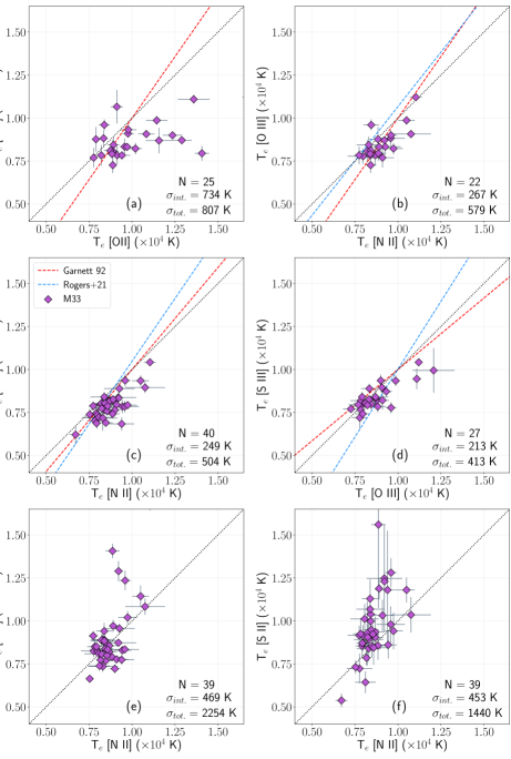
Figure 3: The CHAOS-measured T_e-T_e trends in the H II regions of M33. Each point represents an H II region containing a direct T_e from the corresponding ion. The dashed red and blue lines are the T_e-T_e relations of Garnett (1992) and Rogers et al. (2021), respectively. The number of regions with both direct temperatures, the intrinsic and total scatter in the dependent T_e are provided in the lower right. (a) and (b): The high- vs. low-ionization zone temperatures, the former as measured by T_e[O III] and the latter measured by T_e[O II] (a) and T_e[N II] (b). (c) and (d): Intermediate-ionization zone temperatures from T_e[S III] as compared to T_e[N II] (c) and T_e[O III] (d). (e) and (f): A comparison of the low-ionization zone temperatures measured by T_e[N II] to the temperatures in the same zone as measured from T_e[O II] (e) and T_e[S II] (f).

With the above considerations, we determine the electron temperatures in M33 and report them in Table A.3 in the Appendix. Given the dependence of the electron temperature on the abundance of heavy elements, it is expected that temperatures from different ionization zones are related. When a direct temperature is not measured in an ionization zone, these T_e-T_e relations provide a method to infer the ionization zone temperature from the available temperature data. Many previous studies have derived the functional form of T_e-T_e relations from empirical direct temperature data (e.g., Esteban et al., 2009; Croxall et al., 2016; Arellano-Córdova & Rodríguez, 2020; Rogers et al., 2021) and from photoionization models (e.g., Campbell et al., 1986; Garnett, 1992; Izotov et al., 2006). Many of the H II regions in M33 have multiple direct temperatures, but the size of the sample is not sufficient to derive statistically-significant empirical T_e-T_e relations. Instead, we can compare the direct temperature trends in this galaxy to existing relations.

Figure 3 plots the M33 direct temperature trends from numerous ions and H II regions. Each panel plots the direct temperature from one ion against the temperature from another ion measured in the same region, and each temperature is normalized by 10⁴ K. Reported in the lower right of each panel is the number of H II regions with both direct temperatures, the intrinsic dispersion, defined as the random scatter in the dependent variable about a linear regression fit to the data, and the total dispersion in T_e (both of which are calculated using the same technique as Bedregal et al., 2006). While the intrinsic dispersion depends on which temperature is assumed to be the dependent variable in the linear relation (see discussion in Rogers et al., 2021), we only provide one permutation of the relations because we are not attempting to derive robust relations from the M33 regions alone. We will report on the global direct temperature trends of the CHAOS sample in a future work.

Plotted as a red dashed line in panels (a) and (b) of Figure 3 is the commonly applied low-to-high ionization zone T_e-T_e relation of Campbell et al. (1986); Garnett (1992). In the majority of M33 abundance studies with only T_e[O III], this is the relation applied to obtain the low-ionization zone temperature (see Table 3). As other studies report (Kennicutt et al., 2003; Esteban et al., 2009; Berg et al., 2015; Yates et al., 2020), the trend between the direct temperatures of T_e[O III] and T_e[O II] is not clear and the temperatures are often scattered over many thousands of K. This is true in our sample of temperatures, where panel (a) shows the intrinsic dispersion is significantly larger than the other temperature trends. T_e[N II], another representative temperature of the low-ionization zone, does not show this scatter relative to T_e[O III]. In fact, the direct temperatures measured here follow the Campbell et al. (1986); Garnett (1992) relation well and exhibit small intrinsic scatter.

The observed T_e[O III] in M33, and in many galaxies, have an effective lower limit that is set by the average electron energy within the nebula: the electron energy needed to excite O²⁺ to the 4th excited state is relatively large, requiring either high T_e or a relatively bright region to detect [O III]$\lambda$4363. This prevents detections of low [O III]$\lambda$4363 in all but the brightest regions, which is why there are fewer regions with concurrent T_e[O III] and T_e[N II] in the low-T_e regime ($\lesssim$ 7500 K). The electron energies required to enable the transitions that produce [N II]$\lambda$5755 and [S III]$\lambda$6312 are significantly lower, resulting in the larger number of regions with simultaneous T_e[N II]-T_e[S III] and with T_e $<$ 7500 K in panel (c).

Garnett (1992) also report a photoionization model T_e-T_e relation for the intermediate-ionization zone; the extrapolation of the high-to-intermediate relation to the low-ionization zone is plotted in panel (c). Again, there is generally good agreement between the measured T_e[N II]-T_e[S III] trends in M33 and this relation. The measured temperatures have a small intrinsic dispersion, but the best-fit relation deviates from the relation derived from the other CHAOS galaxies (blue dashed line) at high T_e. The relation reported in Rogers et al. (2021) makes use of 108 direct T_e[N II] and T_e[S III], many of which are at lower average T_e than the T_e measured in M33 (particularly the temperatures from the high-metallicity galaxies NGC 5194 and NGC 3184, see Croxall et al., 2015; Berg et al., 2020). It is not surprising, then, that the temperatures measured here deviate from the trends at the extreme temperature ranges when we do not measure such temperatures in M33.

Panel (d) plots the T_e[S III]-T_e[O III] temperatures observed in 27 regions with the photoionization (Garnett, 1992) and CHAOS empirical T_e[S III]-T_e[O III] relations. The intrinsic dispersion about the M33 relation is a factor of five smaller than that reported in Rogers et al. (2021). Again, the sample of regions examines a relatively small area in T_e-T_e space when compared to the full CHAOS H II region sample, but the large [S III] temperatures measured in other spiral galaxies (like M101, Croxall et al., 2016) are simply not observed in M33. For many regions at moderate T_e, the CHAOS relations describe the T_e trends relatively well.

Finally, panels (e) and (f) focus on the low-ionization zone temperatures from [N II], [O II], and [S II]. Provided that these ions have roughly the same ionization energies, it is expected that their temperatures should be, generally, in agreement. This is roughly the case for the 39 regions with concurrent T_e[N II]-T_e[O II] and T_e[N II]-T_e[S II] where most regions are scattered about the 1-to-1 line. This scatter has been measured in other galaxies (Esteban et al., 2009; Rogers et al., 2021), and it might be related to factors such as dielectronic recombination (Rubin, 1986; Liu et al., 2001), contamination in the NIR, or the presence of higher temperatures in the gas surrounding the H II region (the photodissociation region, or PDR). As such, we deprioritize T_e[O II] and T_e[S II] in the following abundance analysis due to the scatter relative to T_e[N II]. Note that there are actually more T_e[O II] measurements than any other temperature (see Table A.1). A better understanding of the behavior of T_e[O II] would represent a significant increase in diagnostic power.

Following Rogers et al. (2021), we use the weighted-average electron temperature prioritization when calculating the temperature to use in the low-, intermediate-, and high-ionization zones. This method makes use of the available [N II], [S III], and [O III] temperatures in a single region for a robust estimate of the temperature in each ionization zone. With these three temperatures, one can measure a dominant temperature and two inferred temperatures from available T_e-T_e relations, then combine these in a weighted average. This method prioritizes significant T_e from the dominant ion (i.e., those that have the lowest errors in that ionization zone), or a combination of the inferred temperatures when the dominant ion is not detected or is measured at low S/N. We apply the T_e-T_e relations from Rogers et al. (2021), which are calibrated from the CHAOS sample of direct temperatures and employ the intrinsic scatter about the relations to better account for the uncertainties on the inferred temperatures (see discussion in Rogers et al., 2021). If a region does not have significant [N II], [S III], or [O III] auroral line detections, then that region is rejected from the abundance analysis. T_e,Low, T_e,Int, and T_e,High determined from the weight-average prioritization are reported in Table A.3. The following abundance analysis has been repeated using the standard ionization-based temperature prioritization (i.e., use a single direct temperature if it is the dominant ion in the ionization-zone), and all results are consistent within uncertainty.

3.2 ICFs for Various Ionic Species

Table 4: CHAOS Atomic Data

Ion	Transition Probabilities	Collision Strengths
N+	Froese Fischer & Tachiev (2004)	Tayal (2011)
O+	Froese Fischer & Tachiev (2004)	Kisielius et al. (2009)
O2+	Froese Fischer & Tachiev (2004)	Storey et al. (2014)
Ne2+	Froese Fischer & Tachiev (2004)	McLaughlin & Bell (2000)
S+	Irimia & Froese Fischer (2005)	Tayal & Zatsarinny (2010)
S2+	Froese Fischer et al. (2006)	Hudson et al. (2012)
Cl2+	Rynkun et al. (2019)	Butler & Zeippen (1989)
Ar2+	Mendoza & Zeippen (1983)	Munoz Burgos et al. (2009)

Note. — Atomic data used for the calculation of ionic abundances in M33.

With the temperatures in each ionization zone and the intensities of the strong lines available in the optical, we can directly calculate the abundance of different ionic species within each zone via the emissivity of the transition that produces the strong line. The PyNeb getIonAbundance function performs this calculation, where a five-level atom model (De Robertis et al., 1987) is assumed and the atomic data (transition probabilities and collision strengths) are provided in Table 4. To calculate the ionic abundance uncertainty, we propagate the uncertainty on the ionization-zone temperature through the emissivity ratio, then use the resulting emissivity and intensity ratio uncertainty to calculate the total percent error on the ionic abundance. To calculate the total abundance of a given element, it is necessary to obtain an abundance measurement of all ionic species of that element within the H II region. This may not be possible if a specific ionization state has no observable emission lines in the optical, so ICFs are used to account for the unobserved ionic species.

The total abundance of oxygen within an H II region is well-described by O = O⁺ + O²⁺, where it is assumed that there is little neutral O in the H II region due to the coincident ionization energies of H and O. In very highly ionized regions, oxygen can triply ionize; while there are no observable lines of O³⁺ in the optical, significant He II$\lambda$4686 indicates the presence of a very-high ionization zone that contains He²⁺, O³⁺, and other ions (Berg et al., 2021). In the regions of M33, only one region, M33$-$211$-$438, has a significant detection of narrow He II$\lambda$4686; all other regions with significant fits to He II$\lambda$4686 are dominated by the stellar continuum (no clear line, but absorption at 4686 Å predicted by STARLIGHT) or have broad He II$\lambda$4686 indicative of WR stars. While we could account for the missing O³⁺ in M33$-$211$-$438, we adopt the common assumption that all gas-phase O is in the O⁺ or O²⁺ states to remain consistent with the majority of the sample. N⁺ is the only observable ionization state of nitrogen in the optical. N⁺ and O⁺ characterize the low-ionization gas in an H II region, and the ratio of N/O is not expected to change between different ionization zones. The common ICF for N is, therefore, ICF(N) = O/O⁺ such that N/H = N⁺/H${}^{+}\times$ ICF(N). The use of this ICF produces N/O abundances that are found to be within 10% of the true N/O values from photoionization models (see Nava et al., 2006; Amayo et al., 2021).

The ICFs applied for the $\alpha$-element abundances in the CHAOS sample were discussed in Rogers et al. (2021), but these ICFs come from an array of sources (for example, Peimbert & Costero, 1969; Thuan et al., 1995; Izotov et al., 2006). Recently, Amayo et al. (2021) published new ICFs for Ne, S, Cl, and Ar generated from the Mexican Million Models database (3MdB, Morisset et al., 2015). The models used for calibrating the ICFs are selected for their ability to reproduce the line ratios observed in blue compact galaxies and giant H II regions, making them suitable for the sample of regions in M33. Each ICF is a fifth-order polynomial in O²⁺/O and has an associated uncertainty that is itself a polynomial function of O²⁺/O. In prior CHAOS studies it was assumed that the applied ICF had an uncertainty of 10%, but the uncertainty in a given ICF can vary significantly as a function of O²⁺/O (see Figure 7 in Amayo et al., 2021). To accurately calculate the uncertainty in the ICFs, make use of the most recent ICFs, and have a consistent source for all $\alpha$-element ICFs, we use the Ne, S, Cl, and Ar ICFs and their uncertainties from Amayo et al. (2021). These ICFs are calibrated to calculate $\alpha$/O abundances, and so we use the ionic oxygen abundances, when necessary, to convert to $\alpha$/H abundances.

For the first time in a CHAOS abundance study, we determine Cl²⁺ abundances from a significant number of regions (20 total) using the [Cl III]$\lambda\lambda$5517,5537 lines. To determine the ionic abundances, we use the calculated n_e([Cl III]), the [Cl III]$\lambda$5517 intensity, and the intermediate-ionization zone temperature. We require a measure of n_e([Cl III]) to calculate the Cl²⁺ abundance because the assumption of n_e = 10² cm^-3 produces different Cl²⁺/H⁺ when using either [Cl III]$\lambda$5517 or [Cl III]$\lambda$5537 individually. However, the energy levels that produce the [Cl III] density-sensitive lines have higher critical densities than the commonly used [S II] lines; as such, the emissivity ratio of the two lines is a slowly varying function of n_e in the low density regime that describes the regions of M33 (as evidenced by the [S II] lines). In fact, four regions have measured line ratios that are not predicted at the provided T_e in that their ratio is at or above the ratio predicted at n${}_{e}\approx$ 0 cm^-3. For this same reason, the uncertainties calculated using the MCMC method can be particularly large. Taken together, when the line ratio does not permit a calculation of n_e([Cl III]), we calculate Cl²⁺/H⁺ from both lines assuming n_e = 10² cm^-3 and average the resulting values. We have verified that using I([Cl III]$\lambda$5517)$+$I([Cl III]$\lambda$5537) and assuming a density of n_e = 10² cm^-3 produces ionic abundances that are consistent with the ionic abundances determined from the above method. The Cl²⁺/O²⁺ abundance is then used with the Amayo et al. (2021) ICF to determine the Cl/O relative abundance.

4 Abundance Gradients and Dispersions

Using the ionic abundances and ICFs described in the previous section, we calculate the total abundances of numerous elements in M33. We first examine the homogeneous abundances determined from the CHAOS observations to assess the magnitude of the intrinsic dispersion in abundances in M33. In the next section we compare these abundances to the measured literature values and merge the samples that we believe to be of similar quality.

4.1 Oxygen

The third most abundant element, oxygen is a tracer of high-mass star formation. In many star-forming spiral galaxies, the oxygen abundance is observed to be largest near the center of the galaxy and lowest at the edges of the spiral arms. The negative oxygen abundance gradient in M33 measured by C06, R08, B11, and T16 all support the inside-out chemical evolution of this galaxy. The dispersion about the negative abundance gradient is related to processes within the galaxy such as radial motion along spiral arms, local contamination due to pristine gas infall, etc. The scatter measured in M33 from a sample of direct abundances alone ranges between 0.06 dex as measured in the inner 2.2 kpc by B11 to 0.11 dex reported by R08.

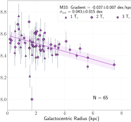
Figure 4: The direct oxygen abundance gradient in M33 measured by CHAOS. The oxygen abundance, 12+log(O/H) (dex), of each region is plotted against the galactocentric radius (in kpc) of the region. The shape of the point represents the number of direct temperatures used to calculate the abundances within the region, as indicated in the legend. The best-fit gradient and intrinsic scatter in O/H about the gradient (provided in the legend) are represented as a solid line and shaded area about the line, respectively.

In Figure 4, we plot the oxygen abundances (in dex) measured in this study against the galactocentric radius of each region in kpc. The linear gradient is fit using the Python LINMIX package, which fits a linear function between two variables while considering the uncertainty in each variable and returns the random scatter in the dependent variable about the linear fit (this is the implementation of the fitting program outlined in Kelly, 2007). The shape of each point in Figure 4 represents the number of direct temperatures used in the weighted-average ionization-zone temperature calculations: triangles indicate regions with a single direct temperature, diamonds represent regions with two, and pentagons are regions with temperatures from [N II], [S III], and [O III]. The shaded region about the gradient represents the intrinsic dispersion (in dex) about the abundance gradient. The gradient and intrinsic dispersion are provided in the legend, and the number of H II regions used in fitting the gradient is found in the lower right corner. The O/H gradient in M33 reported here is measured from 65 H II regions, making this the largest, homogeneous sample of direct abundances in M33.

The gradient measured from this sample is:

$$\mbox{12+log(O/H)}=8.59(\pm 0.02)-0.037(\pm 0.007)\times R_{g,kpc}$$ (1)

where R_g,kpc is the galactocentric radius in kpc. The intrinsic dispersion in oxygen abundance about this gradient is $\sigma_{int}=0.043\pm 0.015$ dex. When normalizing the positions to the effective radius of M33, the gradient is $-$0.081$\pm$0.017 dex/R_e. From Eq. 1, we confirm the existence of a negative oxygen abundance gradient in M33. This abundance gradient appears to accurately describe the O/H trends from within $\sim$0.13 kpc to the outer H II regions at nearly 7.5 kpc.

There is non-negligible scatter in the oxygen abundances, with some regions scattered to relatively low ($\lesssim$ 8.2) and high ($\gtrsim$ 8.7) O/H. However, the scattered regions are primarily those with a single electron temperature used to infer the temperature in all ionization zones; while the uncertainty on O/H is reflective of the missing temperatures, the scatter these regions exhibit highlights the importance of having: 1. High S/N measurements of the T_e-sensitive auroral lines, and 2. Multiple direct temperatures spanning the typical ionization zones of a region.

The measured intrinsic dispersion is less than the value of 0.11 dex reported by R08 and in fairly good agreement with the scatter of 0.06 dex obtained in the inner 2.2 kpc as measured by B11. In fact, the average error in O/H of regions with all three commonly-used electron temperatures is $\langle\delta$(O/H)${}_{3}\rangle=$ 0.053 dex, which matches $\sigma_{int}$ within uncertainty. The average O/H uncertainty for regions with two and one available temperature are $\langle\delta$(O/H)${}_{2}\rangle=$ 0.078 dex and $\langle\delta$(O/H)${}_{1}\rangle=$ 0.118 dex, respectively. Given that intrinsic dispersion in the oxygen abundances is comparable to the average uncertainties of our best measured targets, we find no evidence of significant azimuthal abundance variations in M33.

We examine the distribution of O/H about the best-fit gradient to further explore this claim. If we take $\eta$ to be the difference between the measured and predicted oxygen abundance, where the latter is calculated from Eq. 1 and the radius of the H II region, we can determine its average, $\langle\eta\rangle$, and standard deviation, $\sigma(\eta)$, for the regions with one, two, and three direct temperatures used in the weighted average approach. $\langle\eta\rangle$ examines how the abundances in regions that are missing direct temperatures compare to the best-fit gradient, while $\sigma(\eta)$ provides insight on the scatter in O/H in each sample of regions. We find: for regions with three direct temperatures, $\langle\eta_{3}\rangle=$ 0.00 dex and $\sigma(\eta_{3})=$ 0.05 dex; those with two direct temperatures, $\langle\eta_{2}\rangle=$ 0.03 dex and $\sigma(\eta_{2})=$ 0.10 dex; and for regions with a single temperature, $\langle\eta_{1}\rangle=-$0.04 dex and $\sigma(\eta_{1})=$ 0.11 dex. It is not surprising that the average offset from the gradient is very small for the sample with three direct temperatures, as the uncertainty in O/H is relatively small and the best-fit gradient gives these regions a higher priority in the fit. $\sigma(\eta_{3})$ is consistent with $\langle\delta$(O/H)${}_{3}\rangle$ and $\sigma_{int}$, supporting the claim that the O/H observed in the regions with the highest S/N T_e spanning multiple ionization zones do not show large azimuthal variations.

Our data show evidence that when a single temperature is measured, requiring the use of T_e-T_e relationships to infer the temperature in the other ionization zone, then the dispersion in the total oxygen abundance is inflated because of the inadequacy of simple T_e-T_e relationships to accurately infer temperatures. The temperature most often inferred is the high-ionization zone temperature, as [O III]$\lambda$4363 is detected in 28 regions (see Table A.1). The weighted average approach utilizes the measured T_e[N II] and/or T_e[S III] with the chosen T_e-T_e relations to infer a high-ionization zone temperature, but the T_e[O III]-T_e[S III] relation of Rogers et al. (2021) shows very large scatter and the T_e[O III]-T_e[N II] relation is constructed with a relatively small number of H II regions. A direct measure of T_e within this ionization zone is crucial for reliable measurements of the O²⁺ abundance.

Regions with a single electron temperature rely most on the accuracy of the T_e-T_e relations. Pérez-Montero & Díaz (2003) highlight this weakness in direct abundance measurements, and Arellano-Córdova & Rodríguez (2020) find that applying a single T_e[O III] or T_e[N II] with various T_e-T_e relations can produce differences in total N and O abundances greater than 0.2 dex, especially so when T_e[O III] is inferred from T_e[N II]. While the larger errors on their direct O/H reflect the uncertainty in the relations, the true temperature in a given region/ionization zone can deviate from the simple, linear relations, resulting in erroneous temperatures/abundance trends. Therefore, a measure of the true intrinsic dispersion in O/H within a spiral galaxy can only be obtained with direct measures of the low- and high-ionization zone temperature; the use of inferred temperatures can produce abundances that generally agree with the abundance gradient but show enhanced scatter that is not reflected in the most reliable measurements of T_e and O/H.

4.2 Nitrogen

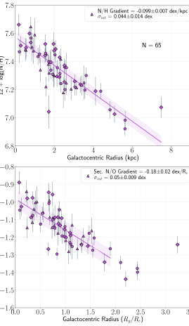
Figure 5: The direct N abundance gradients in M33. In each panel, the gradient and intrinsic scatter are provided as the solid line and shaded regions, respectively, and are reported in the plot legends. The symbols follow the same representation as Figure 4. Top Panel: 12+log(N/H) as a function of R_kpc. Bottom Panel: log(N/O) relative abundances as a function of R_g/R_e, or the galactocentric radius normalized to the effective radius of M33. The gradient and dispersion in this fit are for regions with R_g/R${}_{e}<$ 2 to isolate the secondary N/O gradient.

Nitrogen, which is produced in high-mass stars along with oxygen, has two nucleosynthetic origins: primary nucleosynthesis, in which the ISM is enriched with N via supernovae, and a secondary component where by mass-loss events of intermediate-mass stars releases additional N relative to O and other $\alpha$-elements (Henry et al., 2000). As such, N/H and N/O are relevant quantities to understand the total and secondary enrichment of the ISM with N, respectively.

In the top panel of Figure 5 we plot the N/H abundances against R_g,kpc, where the gradient and dispersion is provided by the solid line and shaded region, respectively, and the symbol representation is the same as Figure 4. All regions with O/H measurements have significant [N II]$\lambda\lambda$6548,6584 detections, hence the number of regions is the same as Figure 4. The 12+log(N/H) gradient in M33 is measured as

$$\mbox{12+log(N/H)}=7.57(\pm 0.02)-0.099(\pm 0.007)\times R_{g,kpc}.$$ (2)

with $\sigma_{int}=0.044\pm 0.014$ dex. The reported intrinsic dispersion in N/H is equivalent to $\sigma_{int}$ about the O/H gradient. This agreement would indicate that the dispersion in O is reflective of the dispersion in other abundant elements in the gas-phase. The total N abundance is related to the O abundance through the ICF(N) $=$ O/O⁺, which might introduce additional scatter into the N/H trends. However, given the agreement between intrinsic dispersions, this effect does not appear to be large enough to produce a larger $\sigma_{int}$ around the N/H gradient.

The N/H gradient is steeper than the O/H gradient because the ISM has been enriched with secondary N. This is easier to visualize in the bottom panel of Figure 5, where we plot the relative abundance of N to O as a function of R_g/R_e, or galactocentric radius normalized to the effective radius of M33. We briefly mention that the N/O gradient determined from LINMIX when using R_kpc is $-0.064\pm 0.007$, which is what one expects if the difference between the N/H and O/H gradients is taken.

Instead of fitting a linear gradient to all regions in M33, we focus on the secondary N/O gradient. We follow the methods of Berg et al. (2020) and fit the N/O abundances at R_g/R${}_{e}<$ 2 with a linear gradient. Berg et al. (2020) show that secondary N production is significant below this radius while N is mostly primary in origin beyond R_g/R${}_{e}=$ 2.5; they also find that three of the CHAOS galaxies exhibit a common secondary N/O gradient of $-$0.34$\pm$0.06 dex/R_e. However, Rogers et al. (2021) measure a significantly shallower secondary N/O gradient of $-$0.16$\pm$0.04 dex/R_e in the spiral galaxy NGC 2403, which was attributed to this galaxy’s lower stellar mass relative to the other CHAOS galaxies. If the stellar mass is a good proxy for the amount of intermediate-mass stars that have enriched the ISM with secondary N, then galaxies with stellar masses similar to NGC 2403 should have similarly shallow secondary N/O gradients.

As shown in the bottom panel of Figure 5, the secondary N/O gradient measured in M33 from the 60 H II regions at R_g/R${}_{e}<$ 2 is:

$$\mbox{log(N/O)}=-0.98(\pm 0.02)-0.18(\pm 0.02)\times R_{g}/R_{e}.$$ (3)

with $\sigma_{int}=0.050\pm 0.009$ dex. The secondary N/O gradient in M33 agrees with that of NGC 2403 when considering uncertainties and is significantly shallower than the common gradient measured in NGC 628, M101, and NGC 3184. The stellar mass of M33 is log(M_⋆/M_⊙) $=$ 9.68 (Corbelli et al., 2014), which is very similar to that of NGC 2403 and supports the possible trend of increasing secondary N/O gradient with increasing stellar mass. We note here that the number of galaxies in this sample size is too small to make any robust claims, and that the N/O gradient can be affected by other factors such as galaxy interaction (Croxall et al., 2015; Berg et al., 2020, see NGC 5194). Furthermore, the Milky Way, with stellar mass log(M_⋆/M_⊙) $=$ 10.78 (Licquia & Newman, 2015), has a N/O gradient that is significantly shallower ($-$0.05$\pm$0.03 dex/R_e, Arellano-Córdova et al., 2020) than that observed in M33.

As a final note, the most extended H II region, M33$-$610$-$1690, appears enhanced in N/O relative to the other extended regions. [N II]$\lambda$5755 is not detected in this region, requiring an inferred low-ionization zone temperature for N⁺/H⁺ abundances. The linear T_e[N II]-T_e[S III] relation constructed from the sample of five CHAOS galaxies in Rogers et al. (2021) is well-sampled and shows low intrinsic dispersion at T${}_{e}<$ 9000 K, but the electron temperatures measured in this region are relatively high: T_e[O III] $=$ 11,100 K and T_e[S III] $=$ 9,500 K. These temperatures are in an area of parameter space not well sampled by the bulk of the CHAOS H II regions and, therefore, the relations might not produce realistic values at such high temperatures. Provided that M33$-$610$-$1690 is the only region at R_g/R${}_{e}>$ 2.5, we fit the primary N/O plateau considering the five regions at R_g/R${}_{e}>$ 2.0 and obtain a weighted-average value of log(N/O)${}_{Primary}=$ $-$1.36, which is in good agreement with the primary N/O plateau measured in M101 by Berg et al. (2020).

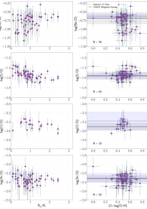
Figure 6: The abundance trends of $\alpha$ elements observed in M33 relative to the oxygen abundance within the region. Left Column: The relative abundances plotted against R_g/R_e. Right Column: The relative abundances plotted against 12+log(O/H). The weighted average and standard deviation of the relative abundances are also provided as black dashed lines and gray shaded regions, respectively. The number of H II regions with the specified relative abundance is provided in the lower left corner. The solar abundance ratios from Asplund et al. (2021) are indicated by blue dotted lines and blue shaded regions, respectively. The rows are ordered by increasing atomic number: First Row: log(Ne/O); Second Row: log(S/O); Third Row: log(Cl/O); Fourth Row: log(Ar/O).

4.3 Neon, Sulfur, Chlorine, and Argon

The elements Ne, S, and Ar are produced in high-mass stars via the alpha-process, the same mechanism that produces O. The production of Cl is controlled by S and Ar, the former through proton capture and the latter through radioactive decay (Clayton, 2003; Esteban et al., 2015). Given their production in the same progenitor stars, the abundance of these four elements should trace the O abundance in an H II region. In Figure 6 we plot the abundance of these elements relative to the oxygen abundance in the regions of M33: the left column plots the relative abundance against R_g/R_e, the right column plots them against 12+log(O/H), and the rows are ordered in increasing atomic number. In the right column, we provide the weighted average log($\alpha$/O) ratio with its standard deviation as a black dashed line and gray shaded region, respectively. We also provide the solar log($\alpha$/O) ratio and its uncertainty from Asplund et al. (2021) as a blue dotted line and blue shaded region, respectively. Note that we no longer represent the H II regions by the number of direct temperatures used in the weighted-average ionization zone temperature calculations.

The first row plots the log(Ne/O) relative abundances, which are scattered over $\sim$1 dex. The Ne²⁺/O²⁺ abundances are calculated directly from the emissivities and line intensities using the high-ionization zone temperature because this temperature describes the gas containing both ions. This approach usually produces small uncertainties on the Ne²⁺/O²⁺ abundances because the emissivity ratio of [Ne III]$\lambda$3868 and [O III]$\lambda$5007 is a weak function of T_e. The large uncertainties on log(Ne/O) come from the ICF(Ne), which is relatively uncertain in regions with O²⁺/O $<$ 0.5. This is also exhibited in the additional scatter at log(Ne/O) $<$ $-$1.0, which is where the ICF is rapidly decreasing at O²⁺/O $<$ 0.2. This matches the trends of the H II region sample used by Amayo et al. (2021); their sample of high-ionization blue compact galaxies show a flat log(Ne/O) trend but we do not observe many H II regions that have this high ionization.

Due to their high uncertainties, the H II regions with low-ionization are not weighted heavily in the calculation of the average log(Ne/O) value. The average log(Ne/O) we measure in M33 is log(Ne/O) $=$ $-$0.69$\pm$0.17 from 56 H II regions. This agrees with the solar value of log(Ne/O) $=$ $-$0.63$\pm$0.06 but note the large uncertainty. If we only consider H II regions with O²⁺/O $>$ 0.2 (in other words, excluding the regions where the ICF is most uncertain and is rapidly changing as a function of O²⁺/O), we determine the average log(Ne/O) from 33 regions to be $-$0.63$\pm$0.10. This exact agreement with the solar value and lack of dependence on R_g/R_e or 12+log(O/H) reveals that Ne enrichment in M33 is consistent with the trends expected for an element produced predominantly by the $\alpha$ process.

All regions with O abundance have the strong lines of S⁺ and S²⁺, producing a sample of 65 S/O abundances in M33. The S ICF corrects the ratio of S⁺ + S²⁺ to O⁺ + O²⁺ to account for missing S³⁺ in high-ionization H II regions. All strong lines in this ratio are measured at high S/N and the ICF is well-constrained over a large range of O²⁺/O, resulting in relatively low uncertainties on the log(S/O) in the second row of Figure 6. While some of the inner regions scatter to slightly high S/O, there is no apparent S/O trend with metallicity. The average value measured in M33 is log(S/O) $=$ $-$1.56$\pm$0.08, in excellent agreement with the solar value of $-$1.57$\pm$0.05.

Only 20 regions have significant [Cl III]$\lambda\lambda$5517,5537 detections, and, in most cases, these emission lines are not detected at high S/N. Furthermore, the uncertainty in the Cl ICF is larger for low-ionization H II regions which produces the large uncertainties observed in a few objects. The Cl/O relative abundances appear constant as a function of R_g/R_e, although there is a slight trend of increasing Cl/O as a function of metallicity. This trend is exhibited in the regions with the lowest uncertainty on Cl/O, and Esteban et al. (2020) obtained a similar Cl/O trend in the H II regions of M101. However, the trend in M101 disappeared depending on the H II region temperature structure assumed. There are not enough regions in the present sample with O/H $<$ 8.3 or $>$ 8.6 to reliably fit this trend which could, ultimately, be a product of the ICF. The average value of log(Cl/O) in M33 is $-$3.51$\pm$0.08. The solar value reported by Asplund et al. (2021), $-$3.38$\pm$0.20, is relatively uncertain because the Cl abundance is determined through HCl observations in sunspot spectra owing to a lack of Cl features in the Sun’s spectrum.

Similar to the strong lines of S, [Ar III]$\lambda$7135 is observed in all regions with O abundance determinations. Provided this line’s high S/N and the potential sky contamination at longer wavelengths, we only use [Ar III]$\lambda$7135 in the calculation of Ar²⁺/O²⁺ abundances. There is no trend in Ar/O as a function of R_g/R_e or 12+log(O/H), and the average determined from the M33 data, $-$2.32$\pm$0.07, is in very good agreement with the solar value, $-$2.31$\pm$0.11. In summary, the abundances of these four elements in M33 appear to be consistent with the enrichment expected for $\alpha$-process or $\alpha$-process-dependent elements and the relative amount of these elements to O is consistent with the solar ratio. Taken together with the O and N abundances discussed above, M33 is chemically well-mixed and homogeneously enriched from inside-out with no evidence of significant abundance variations at a given radius in the galaxy.

5 Literature Comparison

To make the most reliable comparison to the literature direct abundances in M33, we use the line intensities (and their associated uncertainties) and R.A./Decl. centers of each literature H II region, then recompute the temperatures, abundances, and H II region radii in a consistent manner. We do this for all H II regions in M33 from the studies listed in Table 3 using the CHAOS reduction steps explained in §2.2 and §3.2. We apply the S/N $>$ 3 cutoff for detected lines, which does produce fewer auroral line detections and direct abundances in some studies. For example, one region from C06 has a reported [O III]$\lambda$4363 with S/N $<$ 3, resulting in only five regions with T_e[O III]. Similarly, L17 reported abundances for some regions with non-significant [O III]$\lambda$4363 (S/N $<$ 3), and did not report abundances for regions with significant [N II]$\lambda$5755 but non-significant [O III]$\lambda$4363; the net result is that the sample of regions with recalculated direct abundances decreases from 38 to 33.

Most prior studies applied the T_e-T_e relation of Campbell et al. (1986); Garnett (1992) to obtain the low-ionization zone temperature in the H II regions. One exception is T16, who used direct T_e[O III] and T_e[N II] as the high- and low-ionization zone temperatures, respectively, unless T_e[O III] is undetected. In this case, the high-ionization zone temperature is inferred from T_e[N II] and the empirical relation from Esteban et al. (2009), which is in good agreement with the relation used by Campbell et al. (1986) and Garnett (1992). The other exception is A22, who took the same approach as T16 but did not infer any ionization zone temperature; instead, A22 assumed an ionization zone temperature of T_e = 10⁴ K when a direct temperature is missing.

We use the weighted-average temperature approach with the T_e-T_e relations of Rogers et al. (2021) to determine the ionization zone temperature and its uncertainty. For C06, R08, and B11, which do not have the wavelength coverage to measure multiple direct temperatures, this method is simply utilizing the T_e-T_e relations to obtain the electron temperature in the low- and intermediate-ionization zones. For T16, L17, and A22, we use the available T_e[O III] and T_e[N II] to make a robust estimate of the temperature in each zone. Note that no previous abundance study reports T_e[S III] and we still de-prioritize T_e[O II] and T_e[S II], resulting in a weighted average temperature of, at most, one dominant and one inferred T_e in the low- and high-ionization zone.

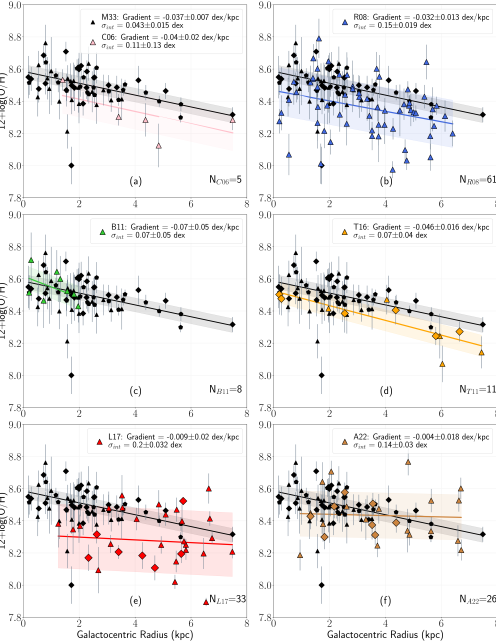
Figure 7: The direct oxygen abundance trends in the M33 H II regions observed by CHAOS (black points with same representation as Figure 4) and the recalculated literature abundance trends (various colored points with same representation). The gradients and intrinsic dispersions in O/H about the gradient are provided in the legends and are plotted as the solid lines and shaded regions, respectively. The number of literature H II regions used in the fits are provided in the lower right corner. The panels provide the recalculated abundances of (a): C06 (pink). (b): R08 (blue). (c): B11 (green). (d): T16 (orange). (e): L17 (red). (f): A22 (brown).

Some studies have reported only one of the [O III] strong lines; while we use [O III]$\lambda$5007 to obtain the O/H abundance in the CHAOS observations of M33, we use [O III]$\lambda$4959 to recalculate the literature abundances if that is the only available [O III] strong line.

In each panel of Figure 7, we plot the oxygen abundances of M33 as measured by CHAOS (black points) and the recalculated literature values (various colors depending on the panel), the best-fit LINMIX abundance gradients determined from these regions (solid colored lines) and the intrinsic dispersion in O/H about the gradients (shaded regions around the solid lines). Again, the shapes indicate the number of direct temperatures used in the weighted average ionization zone temperatures with the same representations as Figure 4. In a few instances, namely for C06 and B11, the LINMIX gradients/dispersions are not well constrained due to the few direct abundances used in the fitting program. Both C06 and B11 combined their observations with existing literature data when fitting their gradient and do not report the gradient from their observations alone due to the small number of regions (C06) or the small radial coverage (B11).

For a better constraint on the gradient and dispersion, we instead fit the recalculated C06 and B11 data with a linear function using the Scipy odr package. This package fits a linear function to the data by minimizing the orthogonal distance of each point to the line of best fit while considering the uncertainties in both dimensions. With the resulting linear fit parameters, we then calculate the intrinsic dispersion about the gradient using LINMIX. In each case, the LINMIX and Scipy odr functions return the same gradient and dispersion, but the uncertainties returned by Scipy odr are more reflective of the data. This technique was repeated for the other literature data compilations, but no difference was measured in the resulting gradients, dispersions, or the uncertainty on either quantity. To remain consistent with the CHAOS approach for M33, the gradients and dispersions in panels (b), (d), (e), and (f) are all calculated using LINMIX.

In general, the recalculated abundances produce gradients that are consistent with the CHAOS-measured gradient. The gradients plotted in panels (a)-(d), which are those reported by studies focusing on the direct and recombination line abundance techniques, agree within uncertainty. Additionally, the intrinsic dispersions about the recalculated C06, B11, and T16 abundance gradients agree with the dispersion about the CHAOS M33 gradient, but are not as well constrained due to the smaller number of regions. The dispersion measured about the gradient in panel (b) from the recalculated R08 abundances is significantly larger than the dispersion measured by CHAOS and is similar to the dispersion originally reported by R08. The reproduction of the intrinsic dispersion in abundance from the R08 line intensity data requires that the atomic data, T_e-T_e relations, and abundance methods are not the source of the large dispersion R08 report.

The primarily strong-line studies plotted in panels (e) and (f) produce direct abundance gradients that are significantly shallower than the CHAOS M33 gradient. Unfortunately, the [O III]$\lambda$4363 line in the inner H II region that L17 report (which they term VGV86 II-063) is not at a high enough S/N to be used in abundance determination, producing a smaller radial coverage and a flatter gradient than originally reported. The regions with T_e[O III] and T_e[N II] tend to scatter low (O/H $<$ 8.2) relative to the CHAOS data. The direct abundances from A22 do appear to be well-distributed within the range of abundances expected from the CHAOS data, although there are a few regions at R${}_{g}>$ 4 kpc with large O/H that flatten the best-fit gradient. A22 label some of these regions as planetary nebula (PNe) based on their position in the classic BPT (Baldwin et al., 1981) diagram. Nine of the H II regions we observe are slightly above the curve that Baldwin et al. (1981) define to designate H II regions and PNe, but we do not observe large scatter in O/H in these regions. All but one of the eight possible PNe that do have direct abundances in our sample have an oxygen abundance consistent with the gradient and the dispersion about it. As such, we do not remove these regions from our sample when reporting the abundance trends in M33.

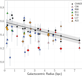
Figure 8: The direct oxygen abundances in the common H II regions of M33 measured by CHAOS (black points) and the literature (other colors, same as Figure 7). The best-fit CHAOS gradient and intrinsic dispersion about the gradient are provided as the solid black line and shaded gray region, respectively. The shape of the points represents the number of direct temperatures used to calculate the abundances, same as Figure 4. H II regions which contain CHAOS abundances but are missing literature abundances are not plotted.

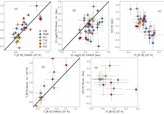
Figure 9: A comparison of the recalculated T_e[O III], T_e[N II], and 12+log(O/H) in the common H II regions observed by the literature studies and CHAOS. Each point is color-coded based on the literature study (see legend). (a): Recalculated T_e[O III] from the literature study vs. the CHAOS T_e[O III] measured in the same region. The black solid line represents a one-to-one relation. (b): Recalculated 12+log(O/H) from the literature study vs. the CHAOS 12+log(O/H). (c): $\delta$(O/H), defined as the difference between the CHAOS and literature oxygen abundances in the same region, vs. $\delta$T_e[O III], the difference between the CHAOS and literature T_e[O III]. (d): Recalculated T_e[N II] from the literature study vs. the CHAOS T_e[N II]. (e): $\delta$(O/H) vs. $\delta$T_e[N II].

Similar regions are targeted in the literature and the present study (see Table 2), allowing for a more direct comparison of the abundances measured in each region. In Figure 8, we plot the CHAOS direct oxygen abundances and gradient in black and the direct oxygen abundances measured in the same H II regions by the literature studies (same colors as Figure 7). In general, the CHAOS oxygen abundances are consistent or larger than the literature abundances for the same H II regions. Additionally, we report a large range of abundances for some of the most well-studied H II regions in M33. For example, three literature studies (R08, B11, T16) observe M33$-$36$-$52, a bright, central H II region that is crucial for constraining the O/H gradient at low radii. The recalculated oxygen abundances for these literature studies and for CHAOS are (O/H)${}_{R08}=$ 8.33$\pm$0.11, (O/H)${}_{B11}=$ 8.72$\pm$0.17, (O/H)${}_{T16}=$ 8.48$\pm$0.10, and (O/H)${}_{CHAOS}=$ 8.54$\pm$0.08, which represent a potential range of $\sim$0.4 dex in abundance between the various studies. We note that the studies with broad wavelength coverage, relatively high spectral resolution, and more than one T_e-sensitive line detected/applied (T16 and this study) agree within uncertainty.

In Figure 9, we attempt to uncover the source of the difference in abundance within these common H II regions and, potentially, the large scatter in the previous abundance studies. In panel (a), we plot the recalculated T_e[O III] against the CHAOS measured T_e[O III] in these regions. Overall, the trend in panel (a) reveals that the literature and CHAOS T_e[O III] track each other relatively well, although there is scatter about the line of unity. This is the case for the majority of the temperatures from R08, where all but one of the common regions has a higher recalculated T_e[O III] when compared to the CHAOS temperatures. Defining the difference between the CHAOS measured and literature T_e[O III] as $\delta$T_e[O III], the average $\delta$T_e[O III] for R08 is $>$ 600 K. There are an additional four common H II regions that contain a recalculated T_e[O III] from the R08 line intensities but in which we fail to detect the [O III]$\lambda$4363 auroral line. This is similar to what B11 finds in their sample of 25 central H II regions: [O III]$\lambda$4363 is undetected in 17 of the H II regions, four of which R08 report a detection of [O III]$\lambda$4363.

Panel (b) plots the recalculated literature oxygen abundances in the common regions against the abundance we report for these regions. The CHAOS abundances are calculated using the available T_e[O III], T_e[S III], and T_e[N II] data, which may result in more regions for comparison relative to panel (a). As Figure 8 makes evident, the recalculated abundances for the literature studies R08 and L17 are scattered lower than the CHAOS abundances. The average $\delta$(O/H), or the difference in direct oxygen abundance between the CHAOS and the literature, is $-$0.12 dex and $-$0.17 dex for R08 and L17, respectively. A22 recalculated abundances are scattered above and below the line of unity, resulting in an average $\delta$(O/H) of $-$0.02 dex. There are too few overlap regions to make a thorough comparison for C06 and B11, but the abundances in the common regions observed by T16 are in excellent agreement with the CHAOS abundances (average $\delta$(O/H) $=$ $-$0.05 dex).

The source of the scatter in panel (b) is explored in panel (c), in which we plot $\delta$(O/H) against $\delta$T_e[O III]. The anti-correlation between $\delta$(O/H) and $\delta$T_e[O III] is clear: the scatter to low oxygen abundances relative to the CHAOS abundances is related to significantly higher T_e[O III] in these regions. This is supported by the two regions from A22 with $\delta$T_e[O III] $<$ 0 and $\delta$(O/H) $>$ 0, and is consistent with the expected trend that electron temperature is anti-correlated with abundance. For three of the literature studies, T_e[O III] ultimately controls the entirety of the oxygen abundance: O²⁺ abundance directly from T_e[O III] and the O⁺ abundance through the inferred low-ionization zone temperature. Significantly different [O III] temperatures should produce noticeably different oxygen abundances, which indicates that the source of the scatter to low abundance is higher T_e[O III]/larger [O III]$\lambda$4363/[O III]$\lambda$5007 intensity ratios in the literature. There is a cluster of regions around $\delta$(O/H) $=$ 0 and $\delta$T_e[O III] $=$ 0 from regions with very similar temperatures and abundances; an exact agreement in temperature may still produce scatter around this location due to slight differences in [O III] strong-line intensities and the applied low- and high-ionization zone temperatures (the latter not necessarily equivalent to T_e[O III] due to the weighted averages).

Panel (d) is the same as panel (a) except the recalculated and CHAOS T_e[N II] are plotted. There is very good agreement between the recalculated T_e[N II] of T16 and those reported in this work. However, the agreement becomes less clear when considering the recalculated temperatures of L17 and A22, where both studies produce slightly larger T_e[N II] than measured from the CHAOS observations. These higher T_e[N II] could be responsible for the flattening of the O/H gradient and the scatter to low O/H observed in both of these studies, although the uncertainties on these T_e[N II] are rather large and, therefore, are not prioritized as much as T_e[O III] in the weighted average ionization zone temperatures.

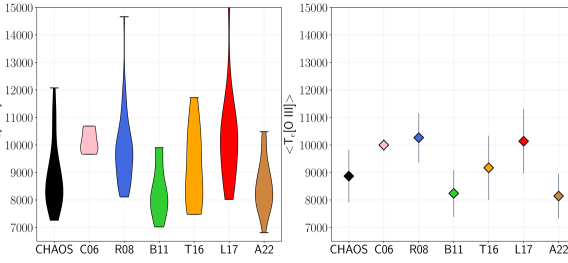
Figure 10: The distribution of T_e[O III] in M33 measured by CHAOS and recalculated from the literature studies. Left Panel: A violin plot of the T_e[O III] measured from the different studies. The minimum, maximum, and number density of T_e[O III] are plotted as the base, peak, and width of each violin, respectively. Some of the violin profiles are affected by the relatively few recalculated T_e[O III] (for example, C06 and T16). Right Panel: The average T_e[O III] and standard deviation measured from the distribution of T_e[O III] in each sample.

The anti-correlation between $\delta$(O/H) and $\delta$T_e[N II] is not as clear in panel (e): while the common regions of T16 are still clustered around the origin, the low number of regions and the larger uncertainties on $\delta$T_e[N II] do not make as convincing a trend. As previously mentioned, the large T_e[N II] uncertainties could produce a low-ionization zone temperature that is weighted more to the inferred temperature from a well-measured T_e[O III]; if this is the case, then the uncertain T_e[N II] has little impact on the final O/H and, therefore, may produce no anti-correlation with O/H.

While we have focused on the common H II regions from the literature and our sample, these high [O III] temperatures are likely the source of the scatter observed in the other literature H II regions. In Figure 10, we plot the distribution of T_e[O III] observed in CHAOS and the literature studies. The violin plot in the left panel shows the minimum, maximum, and number density of T_e[O III] (as minimum, maximum, and width of the violin, respectively) measured in each sample, while the right panel plots each sample’s average T_e[O III] and its standard deviation. We note that 1. We do not expect all T_e[O III] to be in exact agreement because the electron temperature is a function of metallicity and each study targets different H II regions, and 2. That the extreme temperatures affect both the height of the violins and the standard deviation of the average T_e[O III]. The second point is what produces the large standard deviations observed in the right panel, resulting in an agreement between all average T_e[O III]. However, the left panel reveals that the density of T_e[O III] from CHAOS, B11, and A22 all peak at roughly the same temperature. Not only does the density of [O III] temperatures from R08 and L17 peak at higher T_e[O III], but the maximum recalculated T_e[O III] from these samples is larger than observed in any other literature study. Some studies have relatively few recalculated T_e[O III], which impacts their appearance on the violin plot (5 for C06, 8 for B11, and 9 for T16). Of particular note is T16, which shows a relatively constant T_e[O III] density from the minimum to the peak T_e[O III]. This is likely due to the radial and abundance range covered by this sample: T16 measured [O III]$\lambda$4363 in nine H II regions ranging from the center to the outskirts of M33, producing a broad span of T_e[O III] due to the change in O/H but not well-sampled enough to produce a clear peak in the T_e[O III] distribution. Overall, T16 measure a range of [O III] temperatures similar to ours (see also Figure 9).

5.1 A Discussion on the Temperature Dispersion in M33

The remaining question is, then, why are the T_e[O III] from some of the literature studies offset to larger values than we measure in M33? T_e[O III] is dependent on [O III]$\lambda$4363 such that a stronger auroral line produces a larger auroral-to-nebular line ratio which, in turn, results in a higher T_e[O III]. Perhaps the simplest explanation is that noise in the continuum could be interpreted for auroral line emission. If the noise in the continuum is not reflected in the emission line uncertainties and is assumed to be physical, then the reported [O III] auroral line intensities would be biased to larger temperatures resulting in underestimated H II region oxygen abundances.

Alternatively, [O III]$\lambda$4363 can be contaminated by other emission features. One possible source of contamination is [Fe II]$\lambda$4360, which would bias a single fit to [O III]$\lambda$4363 high if unaccounted for (Curti et al., 2017). This is particularly the case if [Fe II]$\lambda$4360 is comparable to a [O III]$\lambda$4363 line that is, on its own, not significant, which might be the situation for high-metallicity H II regions. In this scenario, the auroral line goes from being undetected (with no corresponding direct temperature) to being significantly detected and producing an unrealistically large temperature and low O²⁺ abundance. Provided that many of the studies examined in this work do not have the spectral resolution to fully deblend [Fe II]$\lambda$4360 and [O III]$\lambda$4363, and that these studies did not account for [Fe II] contamination, this is a potential explanation for the scatter towards high T_e[O III]/low O/H.

The degree of significant [Fe II] contamination in M33 that we report in the CHAOS sample is present, but minimal in that few regions have [Fe II]$\lambda$4288 with S/N $>$ 3. Of the nearly 100 regions we observe, only four have significant detections of [Fe II]$\lambda$4288 and, therefore, significant [Fe II]$\lambda$4360 emission that must be accounted for when fitting [O III]$\lambda$4363. As described in §3.1, we subtract the inferred [Fe II]$\lambda$4360 intensity from the intensity of [O III]$\lambda$4363 to account for [Fe II] contamination. This method ensures that [Fe II]$\lambda$4360 is completely removed from [O III]$\lambda$4363 and utilizes a line that is in an area of the continuum that is easy to fit. MODS has a resolution of R $\approx$ 2000 in the blue, which allows for the fit to [Fe II]$\lambda$4360 in cases where the profile of the [O III]$\lambda$4363 line is asymmetric. We have done these fits for all H II regions with asymmetric [O III]$\lambda$4363 and for regions with 2 $<$ S/N([Fe II]$\lambda$4288) $<$ 3 to verify that the profile of [O III]$\lambda$4363 can be trusted.

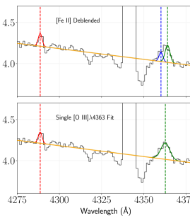
Figure 11: The spectrum of M33$-$35$-$385 near H$\gamma$. The lines [Fe II]$\lambda$4288, [Fe II]$\lambda$4360, and [O III]$\lambda$4363 can be made out in this wavelength range. Top Panel: A fit to the three emission lines while using the [O III] strong lines to constrain the Gaussian FWHM of [O III]$\lambda$4363 and the same FWHM for each [Fe II] line. Each line fit is provided as a colored Gaussian while the linear continuum is plotted as an orange line. [Fe II]$\lambda$4360 and [O III]$\lambda$4363 can be deblended and produces a non-detection of [O III]$\lambda$4363. Bottom Panel: A fit to [Fe II]$\lambda$4288 and a line at 4361.5 Å to simulate a single Gaussian fit to [O III]$\lambda$4363. The Gaussian for [O III]$\lambda$4363 is clearly too intense and too broad relative to the Gaussian with FWHM set by the strong lines, but the intensity is large enough to produce an erroneous line detection.

We plot an example of this in Figure 11, which is the spectrum of the H II region M33$-$35$-$385 focused around H$\gamma$ and [O III]$\lambda$4363. From both panels, there is clear [Fe II]$\lambda$4288 emission and emission at 4363 Å, but the S/N of [Fe II]$\lambda$4288 is less than 3. In the top panel we fit [Fe II]$\lambda$4288, [Fe II]$\lambda$4360, and [O III]$\lambda$4363. To fit the three lines in the top panel, we first fit the [O III] strong lines to obtain the FWHM of the Gaussians in km/s, then use this to obtain the FWHM of the [O III]$\lambda$4363 Gaussian. We then assume that the [Fe II] lines have the same FWHM and that their flux ratio must be equivalent to the emissivity ratio of the two transitions. The fit to [Fe II]$\lambda$4360 and [O III]$\lambda$4363 captures the asymmetric profile and one can clearly see the contamination from [Fe II]$\lambda$4360 despite the fact that [Fe II]$\lambda$4288 is measured at 2 $<$ S/N([Fe II]$\lambda$4288) $<$ 3. The bottom panel plots the fit to [Fe II]$\lambda$4288 and [O III]$\lambda$4363 assuming that there is a single line at 4361.5 Å and allowing for the Gaussian FWHM of each line to vary freely. The intensity and width of the line at 4361.5 Å is clearly too large relative to the deblended fit in the top panel, which would be the scenario if the resolution of MODS was insufficient to deblend [Fe II]$\lambda$4360 and [O III]$\lambda$4363. The fit in the top panel produces a non-detection in [O III]$\lambda$4363 while the bottom panel is at sufficiently high signal to produce a detection, which would bias the T_e[O III] and ionization-zone temperatures in this region to unphysically large values.

We propose an additional explanation for the high T_e[O III] in some of the literature studies: contamination from the night sky. The redshift of M33, z $=-$0.000597, is particularly troublesome for direct abundance studies that rely solely on [O III]$\lambda$4363. At this redshift, [O III]$\lambda$4363 is blueshifted from its theoretical wavelength to $\lambda$4360.60 Å (with individual H II regions shifted up to $\pm$ $\sim$ 2Å due to the rotation of the galaxy; Koch et al., 2018) which is in close proximity to the Hg I night sky line at $\lambda$4358.34 Å. If there is prominent Hg I night sky emission and the spectral resolution of the detector is not sufficient, these two lines could be partially or totally blended. Hg I $\lambda$4358 is observed at the LBT, but the resolution is sufficient that the night sky line can be cleanly subtracted in most cases. As described in §3.1, in cases where the profile of [O III]$\lambda$4363 is asymmetric or there is evidence of poor subtraction of the Hg I line, we fit the sky residuals to the blue side of [O III]$\lambda$4363 and exclude this emission from the flux of [O III]$\lambda$4363. This approach was originally taken for potential significant [Fe II] contamination, but it works for a Hg I $\lambda$4358 undersubtraction artifact because this noise is shifted to 4360.9 Å when the spectrum is redshift corrected.

Hg I contamination of [O III]$\lambda$4363 will typically produce [O III] temperatures that are biased higher than the actual [O III] temperature in the region. Consider a spectrum with insufficient resolution to completely deblend Hg I $\lambda$4358 and [O III]$\lambda$4363 in M33. There are two scenarios of contamination, one in which the Hg I line is oversubtracted and another in which the line is undersubtracted. In the first case, the oversubtraction of Hg I clips the [O III] auroral line and produces negative residuals on the blue side of the otherwise Gaussian profile. In cases of extreme contamination, the loss in [O III]$\lambda$4363 flux will produce a S/N $<$ 3 and cause the auroral line to go undetected. In the second scenario, an undersubtraction still produces a non-Gaussian profile but increases the flux in the fit for [O III]$\lambda$4363. When contamination is large, the additional flux could cause an otherwise undetected [O III]$\lambda$4363 to be fit at a S/N $>$ 3, but even small amounts of contamination will bias the [O III] flux/temperature high. In this way, Hg I contamination removes all 4363 when the oversubtraction is significant but increases 4363 when there is any undersubtraction in the line, producing a net trend to higher [O III] flux.

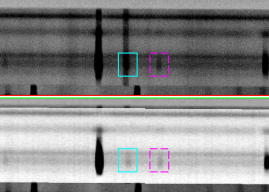
Figure 12: A portion of the MODS 2D spectrum of M33+29+261 focused on H$\gamma$, Hg I $\lambda$4358, [O III]$\lambda$4363, He I $\lambda$4388, and He I $\lambda$4471. Top Panel: The 2D spectrum before sky subtraction. The location of [O III]$\lambda$4363 is highlighted in the cyan box and the line can be seen on the red edge of the Hg I $\lambda$4358 emission. With lower spectral resolution, [O III]$\lambda$4363 may be entirely blended with Hg I $\lambda$4358. The location of He I $\lambda$4388 is highlighted with the dashed magenta box. Bottom Panel: The 2D spectrum after sky subtraction. Hg I $\lambda$4358 is cleanly subtracted and the [O III]$\lambda$4363 emission is present within the cyan box. The 2D profile of [O III]$\lambda$4363 is comparable to the He I $\lambda$4388 feature, the latter of which is not susceptible to Hg I contamination.

The potential Hg I contamination in the literature spectra of M33 is dependent on: 1. The resolution of the detector, and 2. Whether or not Hg I emission is present in the sky at the telescope location. For instance, the raw data obtained from the GTC used by T16 show evidence of Hg I $\lambda$4358, but the resolution of the R2500U grism is sufficient enough to clearly separate this line from [O III]$\lambda$4363. An example of a MODS 2D spectrum obtained from the multi-object field observation of M33+29+261 is provided in Figure 12. The top panel is the spectrum before sky subtraction, while the bottom is the spectrum after sky subtraction (the limits are unchanged between the panels). We focus on the portion of the spectrum from H$\gamma$, the intense line to the left of the cyan box, to He I $\lambda$4471. The locations of [O III]$\lambda$4363 and He I $\lambda$4388 are highlighted by the solid cyan box and dashed magenta box, respectively, in both panels. In the top panel, the Hg I sky line spans the entire slit and is close in proximity to [O III]$\lambda$4363, but it is possible to make out the red edge of the auroral line. In the bottom panel, Hg I $\lambda$4358 line is cleanly subtracted and the [O III] auroral line emission is still detectable. Furthermore, the 2D profile of [O III]$\lambda$4363 is comparable to the He I $\lambda$4388 profile in the dashed magenta box. This line is not affected by Hg I or night sky contamination, therefore the similar profile of the [O III] auroral line would indicate negligible sky contamination in the MODS spectrum.

Detectors with insufficient spectral resolution, however, could be subject to the night sky or [Fe II] contamination. This could be a potential explanation for the scatter to high T_e[O III] observed in the recalculated L17 temperatures: the resolution of $\sim$6 Å of Hectospec at the MMT might be insufficient to deblend the [O III] auroral line and night sky line, in which case the contamination will bias the [O III] flux and T_e high. The same is true for R08, who obtained their raw spectra using LRIS on Keck I, but the degree to which Hg I $\lambda$4358 is present at Mauna Kea would favor [Fe II] contamination. The agreement between the CHAOS and T16 [O III] and [N II] temperatures, the latter of which are free from these sources of contamination, indicate that high-S/N observations with multiple T_e-sensitive auroral lines produce the same abundance gradient and similarly low scatter in abundance. This highlights the importance of high spectral resolution to distinguish various emission lines, and large wavelength coverage to properly measure the temperatures in different ionization zones in an H II region and to avoid a reliance on a single, potentially contaminated T_e measurement.

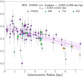
Figure 13: The oxygen abundance gradient in M33 as measured from CHAOS (65 regions, purple), T16 (6 regions, orange), A22 (13 regions, green), and Esteban et al. (2009) (2 regions, cyan). The best-fit gradient (dashed purple line) and intrinsic dispersion in O/H (shaded purple area) are provided in the legend. The point representation is the same as Figure 4.

We believe the homogeneity of the CHAOS sample makes for the most reliable measurement of properties such as the intrinsic dispersion about the abundance gradient. Nonetheless, we determine the impact on the oxygen abundance gradient and dispersion when we combine the CHAOS abundances with those from the literature with similar wavelength coverage, spectral resolution, and direct temperature measurements. These studies include T16, A22, and the abundances of NGC 604 and NGC 595 from Esteban et al. (2009), which have been recalculated in the same manner as the other literature samples. Esteban et al. (2009) used the Keck High Resolution Echelle Spectrometer (HIRES), which has a spectral resolution of R$\approx$23,000 (for their configuration) and is sufficient to deblend any potential [O III]$\lambda$4363 contaminators. In constructing the combined M33 sample, we exclude the PNe objects from A22 due to the unexplained scatter to high O/H that we do not observe. In cases of overlap regions, we prioritize our homogeneous sample, followed by T16, Esteban et al. (2009), and finally A22. The sample of 86 H II regions is plotted as a function of radius (in kpc) in Figure 13, and the resulting best-fit O/H gradient is $-$0.043$\pm$0.006 dex/kpc with intrinsic dispersion $\sigma_{int}=$ 0.057$\pm$0.012 dex. Despite the increase in the slope of the composite gradient due to the inclusion of the low abundances observed in the outer H II regions by T16 (see panel d in Figure 7), both the gradient and intrinsic dispersion agree with the values obtained from the homogeneous CHAOS sample.

5.2 The Abundance Dispersion in Local Spirals

The dispersion in O/H measured about the abundance gradient in a spiral galaxy is related to the presence/absence of mixing mechanisms within the galaxy. Various mechanisms affect gas motion and mixing on different time and spatial scales (see discussion in Roy & Kunth, 1995). The observation of low dispersion about an abundance gradient is indicative of effective mixing mechanisms that distribute the heavy elements after local enrichment from stellar nucleosynthesis. On the contrary, large abundance variations indicate that local enrichment is dominant, i.e. that the mechanisms acting to homogenize the ISM are inefficient or not present. From the large sample of regions in M33, the dispersion in O/H is relatively low/consistent with the observational uncertainties on the most well-measured abundances. The subsample of regions with the direct T_e from [O III], [S III], and [N II] (22 regions) support this further, as the standard deviation about the gradient from these regions is $\sim$0.05 dex (see §4.1). The other CHAOS galaxies show similarly low dispersion, ranging from $\sim$0.04 dex to 0.10 dex (Rogers et al., 2021).

Recently, Esteban et al. (2022) examined the abundances in the Galaxy as measured from a number of sources, including H II regions from Arellano-Córdova et al. (2020, 2021), with the goal of assessing the large abundance dispersion that De Cia et al. (2021) measure in Galactic neutral clouds. The direct abundances in the H II regions are calculated using T_e[N II] in the low-ionization zone and T_e[O III] in the high-ionization zone, only applying the Esteban et al. (2009) T_e-T_e relation when one of these temperatures is missing. From the 42 Galactic regions, the dispersion about the O/H gradient is $\sim$0.07 dex, which is similar to the dispersion in metallicity measured from B-type stars, classical Cepheids, and young clusters in the Galaxy (Esteban et al., 2022), and significantly less than the dispersion measured in the neutral clouds. Méndez-Delgado et al. (2022a) corroborate the low dispersion in the Arellano-Córdova et al. (2020, 2021) H II regions when considering non-zero temperature fluctuations and updated H II region positions. In the spiral galaxy M101, Kennicutt et al. (2003) determine the abundance gradient from 20 H II regions, the majority of which have direct T_e[O III] and T_e[S III] measurements and nine have direct T_e[N II]. Citing the tight correlation they observe between T_e[O III] and T_e[S III], Kennicutt et al. (2003) use an average of the direct T_e[O III] and the inferred T_e[O III] from T_e[S III] to obtain the high-ionization zone temperature and they use the direct T_e[N II] in the low-ionization zone, when available. Although this sample consists of only 20 regions, there is a clear abundance gradient in M101 with very little dispersion about the gradient. The dispersion reported by CHAOS (0.097 dex, Rogers et al., 2021) is slightly larger than the gradient from Kennicutt et al. (2003) would indicate, but this could be due to the inclusion of H II regions with a single direct T_e.

Taken together, the magnitude of the intrinsic dispersion in O/H observed in local spiral galaxies would suggest the following: 1. Large abundance variations are not typically observed when considering the H II regions with the most reliable abundance measurements; 2. The mixing mechanisms in these galaxies act to efficiently homogenize the ISM such that the dispersion is at the level of observational uncertainty; 3. The use of single-temperature H II regions has the potential to inflate the measured intrinsic dispersion to unphysically large values, erroneously suggesting that local enrichment/pollution are dominant relative to the mixing mechanisms. As discussed in §5.1, the use of a single T_e[O III] in M33 is particularly problematic due to various contaminating sources, which might explain the abundance scatter reported in previous studies. That being said, any H II region could have a temperature structure that deviates slightly from the predicted T_e-T_e relations and can result in large abundance variations (Arellano-Córdova & Rodríguez, 2020). Robust T_e-T_e relations that account for other properties of the region (hardness of the ionizing radiation, metallicity, etc.) may improve inferred temperature estimates, but the simple linear relations have the potential to inflate abundance dispersion when only one temperature is applied. Strong line abundance calibrators have been shown to produce lower abundance variations relative to the direct technique when a single direct temperature is used (see Arellano-Córdova et al., 2016). However, empirical and theoretical strong line calibrators can produce different abundances, gradients, and dispersions in the same galaxy (Kewley & Ellison, 2008; Moustakas et al., 2010). Therefore, for the most accurate measure of the abundance dispersion in a galaxy it is imperative to have direct temperature measurements across multiple ionization zones in a significant number of H II regions.

6 Conclusions

We report on the CHemical Abundances Of Spirals observations of the well-studied spiral galaxy M33. Of the nearly 100 H II regions targeted, we detect significant temperature-sensitive auroral line emission from [O III], [N II], or [S III] in 65 regions, as well as emission from the auroral lines of [O II], [S II], and [Ar III]. We also detect [Cl III]$\lambda\lambda$5517,5537 in 20 regions, allowing for the first statistically significant Cl abundance determination in a CHAOS galaxy. [Fe II]$\lambda$4288 is significantly detected in 4 H II regions, indicating that [Fe II]$\lambda$4360 contamination of [O III]$\lambda$4363 must be accounted for in these regions, but that the degree [Fe II] contamination is, in general, fairly minimal in M33.

The temperatures we measure in M33 show little scatter and generally follow the existing literature T_e-T_e relations. We use the direct temperatures from [O III], [N II], and [S III] and the T_e-T_e relations and weighted-average ionization zone temperature approach from Rogers et al. (2021). The ionization zone temperatures are used to obtain the ionic abundances of many species in M33; the oxygen abundances measured in 65 H II regions constitute the largest homogeneous sample of direct abundances in M33 to date.

From multiple elements, the chemical enrichment of M33 is homogeneous and shows little dispersion, indicating a well-mixed ISM. The intrinsic dispersion measured about the oxygen abundance gradient is consistent with the uncertainty on the most well-measured O/H. The scatter observed in the subsample of regions with direct temperatures of T_e[O III], T_e[S III], and T_e[N II] is 0.05 dex, while the scatter measured in regions with fewer direct T_e is closer to $\sim$0.11 dex. The secondary N/O gradient in M33 is shallower than the universal secondary N/O gradient reported in Berg et al. (2020), but is consistent with the gradient measured in other spiral galaxies with low stellar mass. The $\alpha$-process and $\alpha$-process-dependent elements show averages consistent with the solar values and do not vary as a function of galactocentric radius.

We compare our results to literature studies that measure oxygen abundance gradients in M33. While the total literature abundance sample is one of the largest in any spiral galaxy, it is obtained in an inhomogeneous manner (i.e., different detectors, wavelength coverage, and temperatures used) and a complete and consistent recalculation of temperatures and abundances is required to make a one-to-one comparison. We use the reported line intensities and complete this re-reduction, then compare the resulting temperatures and abundances to the CHAOS-measured values. While there is generally good agreement between the gradients determined from primarily direct-abundance studies, the direct abundance gradients determined from the primarily strong line studies are significantly shallower and have much larger dispersions.

Comparing the physical properties in common H II regions, we find very good agreement with the [O III] and [N II] temperatures and O/H abundances measured by T16. The differences in O/H relative to the other literature studies are related, primarily, to the difference in T_e[O III]. We discuss different mechanisms for [O III]$\lambda$4363 contamination, such as from [Fe II]$\lambda$4360 or the Hg I $\lambda$4358 sky line, which is a unique source of contamination for M33 due to its redshift. The use of low-resolution spectrographs can blend [O III]$\lambda$4363 with these contaminating sources and produce unphysical T_e[O III]; using relatively high-resolution spectroscopy with broad wavelength coverage, sufficient to obtain electron temperatures from multiple ionization zones, is the only way to avoid, or limit the impact of, contamination.

The result that M33 is chemically well-mixed and shows little abundance variations is supported by the studies that meet the above criteria. Similar abundance studies that detect multiple temperatures from numerous H II regions in local spiral galaxies also show intrinsic dispersions that are consistent with observational uncertainties. These findings suggest that the ISM is well-mixed in these galaxies and that the use of single-temperature regions can inflate the dispersion in O/H. Studies seeking to obtain the most accurate measure of the variation in O/H should strive to directly measure T_e in multiple ionization zones to avoid any potential biases associated with the application of linear T_e-T_e relations or contamination in the single temperature.

We thank the referee for their thorough review of the original manuscript and the useful feedback that has improved the clarity of this work. This work has been supported by NSF Grants AST-1109066 and AST-1714204. This paper uses data taken with the MODS built with funding from NSF grant AST-9987045 and the NSF Telescope System Instrumentation Program (TSIP), with additional funds from the Ohio Board of Regents and the Ohio State University Office of Research. This paper made use of the modsIDL spectral data reduction pipeline developed in part with funds provided by NSF Grant AST-1108693 and a generous gift from OSU Astronomy alumnus David G. Price through the Price Fellowship in Astronomical Instrumentation. This work was based in part on observations made with the Large Binocular Telescope (LBT). The LBT is an international collaboration among institutions in the United States, Italy and Germany. The LBT Corporation partners are: the University of Arizona on behalf of the Arizona university system; the Istituto Nazionale di Astrofisica, Italy; the LBT Beteiligungsgesellschaft, Germany, representing the Max Planck Society, the Astrophysical Institute Potsdam, and Heidelberg University; the Ohio State University; and the Research Corporation, on behalf of the University of Notre Dame, the University of Minnesota, and the University of Virginia. This research has made use of the NASA/IPAC Extragalactic Database (NED) which is operated by the Jet Propulsion Laboratory, California Institute of Technology, under contract with the National Aeronautics and Space Administration. This study has made use of the GTC Archive; the GTC Archive is part of the Spanish Virtual Observatory project funded by MCIN/AEI/10.13039/501100011033 through grant PID2020-112949GB-I00

In this Appendix, we provide the following information: Emission Line Detections are reported in Table A.1; Line Intensities are provided in Table A.2; and the Temperatures and Abundances in each region are listed in Table A.3.

Table A.1: M33 Emission Line Detections

H II	Auroral Lines						Other Lines				Wolf
Region	[O III]	[N II]	[S III]	[O II]	[S II]	[Ar III]	C II	[Cl III]	[Ar IV]	[Fe II]	Rayet
Total Detections:	28	42	62	84	64	5	10	20	4	4
M33$-$2+25				✓
M33+23$-$9		✓	✓		✓						✓
M33$-$23+16
M33$-$28+6	✓	✓	✓	✓	✓			✓
M33$-$36$-$52		✓	✓	✓	✓
M33+2+111			✓	✓
M33$-$6$-$120			✓	✓
M33+78+91		✓	✓	✓	✓
M33$-$89$-$21				✓	✓
M33$-$42$-$138
M33+108+25				✓
M33$-$66$-$161		✓	✓	✓	✓		✓
M33$-$114$-$123
M33+89+165		✓	✓	✓	✓
M33$-$88$-$166			✓	✓	✓
M33+125+78	✓	✓	✓	✓	✓
M33$-$89+89			✓	✓
M33$-$144$-$78		✓		✓	✓
M33$-$150$-$79				✓	✓
M33+70+228		✓		✓	✓
M33+29+261	✓	✓	✓	✓	✓		✓	✓
M33+135+264	✓	✓	✓	✓	✓			✓
M33+146+266			✓	✓
M33+143+328				✓
M33$-$24$-$333
M33+113$-$224		✓	✓	✓	✓
M33+69+352		✓	✓	✓	✓
M33+88$-$258				✓							✓
M33+62+354	✓	✓	✓	✓	✓		✓	✓
M33$-$36+312			✓	✓	✓
M33$-$2$-$340			✓	✓	✓
M33$-$65+302
M33$-$108$-$389			✓	✓	✓
M33+14$-$355				✓
M33+33+382	✓		✓
M33$-$35$-$385		✓	✓	✓	✓			✓
M33$-$78+311			✓	✓	✓
M33+116$-$286			✓	✓	✓
M33$-$99+311	✓	✓	✓	✓	✓			✓
M33$-$148$-$412		✓	✓	✓	✓
M33$-$196$-$396				✓	✓
M33+122$-$294				✓	✓
M33+26+421				✓	✓
M33+46$-$380	✓	✓	✓	✓	✓			✓			✓
M33+126$-$313	✓		✓	✓	✓
M33$-$77$-$449			✓	✓
M33$-$168$-$448			✓	✓	✓
M33+175+446		✓	✓	✓	✓
M33$-$211$-$438	✓	✓	✓	✓	✓
M33$-$224$-$437		✓	✓	✓	✓
M33+253$-$141
M33+19+466		✓	✓	✓	✓
M33+263+423				✓
M33+209+473	✓	✓	✓	✓	✓		✓	✓			✓
M33+285+399
M33+221+476				✓
M33$-$263$-$461		✓	✓	✓				✓
M33$-$267$-$462		✓	✓	✓	✓						✓
M33$-$128+386	✓	✓	✓	✓
M33$-$143+371
M33+285+456				✓
M33+267$-$191			✓	✓	✓
M33+121$-$405	✓	✓	✓	✓	✓			✓			✓
M33+300+471				✓	✓
M33+266$-$221				✓
M33+299$-$164			✓	✓
M33+208+567	✓	✓	✓	✓	✓		✓	✓
M33+94+574		✓	✓	✓	✓
M33+107+581		✓	✓	✓	✓
M33+322$-$139	✓	✓	✓	✓	✓			✓
M33+119+592				✓
M33+299+541			✓	✓	✓
M33+334$-$135	✓	✓	✓	✓	✓		✓
M33+328+543				✓
M33+306$-$276			✓	✓
M33+369+545				✓
M33+380+578				✓
M33+400+552				✓	✓
M33+405+554		✓	✓	✓	✓
M33+298$-$344	✓	✓	✓	✓	✓
M33+421+560					✓
M33+313$-$342			✓	✓	✓
M33+325$-$329
M33+330$-$345
M33+345$-$344		✓	✓	✓	✓			✓
M33+333+745	✓	✓	✓	✓	✓	✓	✓	✓	✓	✓	✓
M33+417$-$254				✓	✓
M33+371$-$348	✓			✓	✓
M33+388$-$320
M33+541+448	✓	✓	✓	✓	✓	✓	✓	✓		✓	✓
M33+553+448	✓	✓	✓	✓	✓	✓	✓	✓	✓	✓	✓
M33$-$464+348	✓		✓	✓	✓
M33$-$507+346	✓	✓	✓	✓	✓			✓
M33$-$72$-$1072	✓	✓	✓	✓	✓			✓
M33$-$181$-$1156	✓		✓	✓	✓
M33$-$438+800	✓	✓	✓	✓	✓	✓	✓	✓	✓	✓
M33$-$442+797	✓	✓	✓	✓	✓	✓		✓	✓
M33$-$610$-$1690	✓		✓	✓	✓

Note. — Emission line detections in the H II regions of M33. A checkmark indicates an emission line that is measured at S/N $>$ 3. Column 1: H II region ID. Columns 2-7: Temperature-sensitive auroral line detections in the H II region. The auroral lines are [O III]$\lambda$4363 (Col. 2), [N II]$\lambda$5755 (Col. 3), [S III]$\lambda$6312 (Col. 4), [O II]$\lambda\lambda$7320,7330 (Col. 5), [S II]$\lambda\lambda$4069,4076 (Col. 6), and [Ar III]$\lambda$5192 (Col. 7). Columns 8-11: Significant detections of other physically-significant emission lines which include: C II $\lambda$4267 (Col. 8), [Cl III]$\lambda\lambda$5517,5537 (Col. 9), [Ar IV]$\lambda$4740 (Col. 10), and [Fe II]$\lambda$4288 (Col. 11). Column 12: Wolf-Rayet features observed in the region.

Table A.2: M33 Emission Line Intensities

$I(\lambda)/I(\mbox{H}\beta)$
Ion	M33$-$2+25	M33+23$-$9	M33$-$23+16	M33$-$28+6	M33$-$36$-$52	M33+2+111	M33$-$6$-$120	M33+78+91	M33$-$89$-$21
[O ii] $\lambda$3727	2.799$\pm$0.180	1.389$\pm$0.089	1.906$\pm$0.142	2.138$\pm$0.151	1.989$\pm$0.140	2.172$\pm$0.059	3.217$\pm$0.296	2.161$\pm$0.055	2.444$\pm$0.139
H13 $\lambda$3734	0.027$\pm$0.004	0.027$\pm$0.006	0.030$\pm$0.008	0.030$\pm$0.003	0.026$\pm$0.003	29.4$\pm$1.8$\times$10-3	0.028$\pm$0.006	27.0$\pm$2.0$\times$10-3	0.030$\pm$0.002
H12 $\lambda$3750	0.030$\pm$0.011	0.047$\pm$0.006	0.053$\pm$0.017	0.039$\pm$0.004	0.036$\pm$0.003	0.044$\pm$0.004	0.028$\pm$0.017	0.033$\pm$0.008	0.057$\pm$0.008
H11 $\lambda$3770	0.046$\pm$0.009	0.058$\pm$0.004	0.056$\pm$0.013	0.047$\pm$0.004	0.043$\pm$0.004	0.047$\pm$0.005	0.036$\pm$0.012	0.047$\pm$0.004	0.060$\pm$0.006
H10 $\lambda$3797	0.060$\pm$0.008	0.060$\pm$0.013	0.066$\pm$0.016	0.064$\pm$0.007	0.057$\pm$0.006	0.064$\pm$0.004	0.059$\pm$0.013	0.058$\pm$0.004	0.065$\pm$0.005
He I $\lambda$3819	0.015$\pm$0.009	$\cdots$	0.013$\pm$0.015	0.017$\pm$0.004	0.011$\pm$0.003	0.011$\pm$0.003	0.017$\pm$0.006	0.013$\pm$0.003	0.002$\pm$0.002
H9 $\lambda$3835	0.078$\pm$0.010	0.097$\pm$0.007	0.102$\pm$0.014	0.091$\pm$0.007	0.089$\pm$0.006	0.088$\pm$0.007	0.084$\pm$0.011	0.102$\pm$0.009	0.098$\pm$0.006
[Ne iii] $\lambda$3868	0.010$\pm$0.008	0.002$\pm$0.003	0.021$\pm$0.016	0.115$\pm$0.008	0.046$\pm$0.003	0.014$\pm$0.004	0.028$\pm$0.012	0.021$\pm$0.003	0.000$\pm$0.002
He I $\lambda$3888	0.092$\pm$0.012	0.070$\pm$0.008	0.105$\pm$0.018	0.111$\pm$0.013	0.114$\pm$0.012	0.070$\pm$0.004	0.099$\pm$0.020	0.098$\pm$0.008	0.072$\pm$0.009
H8 $\lambda$3889	0.115$\pm$0.016	0.118$\pm$0.025	0.126$\pm$0.031	0.122$\pm$0.013	0.110$\pm$0.011	0.124$\pm$0.008	0.113$\pm$0.025	0.112$\pm$0.008	0.124$\pm$0.010
He I $\lambda$3964	$\cdots$	0.006$\pm$0.009	$\cdots$	0.009$\pm$0.007	0.008$\pm$0.008	0.007$\pm$0.003	0.001$\pm$0.006	0.010$\pm$0.004	0.001$\pm$0.008
[Ne iii] $\lambda$3967	$\cdots$	$\cdots$	0.012$\pm$0.020	0.046$\pm$0.010	0.013$\pm$0.008	$\cdots$	0.012$\pm$0.014	0.034$\pm$0.004	$\cdots$
H7 $\lambda$3970	0.170$\pm$0.024	0.176$\pm$0.038	0.184$\pm$0.046	0.177$\pm$0.019	0.163$\pm$0.017	0.184$\pm$0.011	0.165$\pm$0.036	0.164$\pm$0.012	0.184$\pm$0.015
He I $\lambda$4026	0.003$\pm$0.010	0.003$\pm$0.003	0.016$\pm$0.009	0.024$\pm$0.002	19.7$\pm$1.7$\times$10-3	0.014$\pm$0.004	0.005$\pm$0.024	0.012$\pm$0.005	0.013$\pm$0.003
[S ii] $\lambda$4068	0.013$\pm$0.009	6.4$\pm$1.6$\times$10-3	0.003$\pm$0.008	0.009$\pm$0.002	11.0$\pm$1.5$\times$10-3	0.007$\pm$0.003	0.017$\pm$0.009	0.019$\pm$0.005	0.018$\pm$0.003
[S ii] $\lambda$4076	$\cdots$	2.8$\pm$1.6$\times$10-3	0.014$\pm$0.010	0.003$\pm$0.002	3.6$\pm$1.5$\times$10-3	0.001$\pm$0.003	0.013$\pm$0.008	0.008$\pm$0.005	0.006$\pm$0.003
H$\delta$ $\lambda$4101	0.260$\pm$0.017	0.254$\pm$0.010	0.255$\pm$0.014	0.268$\pm$0.011	0.273$\pm$0.012	0.258$\pm$0.011	0.285$\pm$0.013	0.268$\pm$0.012	0.261$\pm$0.012
He I $\lambda$4120	$\cdots$	0.006$\pm$0.007	0.004$\pm$0.011	0.1$\pm$1.9$\times$10-3	1.8$\pm$1.7$\times$10-3	1.7$\pm$1.5$\times$10-3	0.003$\pm$0.006	$\cdots$	$\cdots$
He I $\lambda$4143	$\cdots$	0.001$\pm$0.002	0.009$\pm$0.010	0.000$\pm$0.002	3.1$\pm$1.8$\times$10-3	0.000$\pm$0.003	$\cdots$	$\cdots$	$\cdots$
C II $\lambda$4267	0.007$\pm$0.007	$\cdots$	$\cdots$	0.002$\pm$0.002	14.2$\pm$9.2$\times$10-4	$\cdots$	0.010$\pm$0.006	0.002$\pm$0.004	$\cdots$
[Fe II]$\lambda$4288	0.001$\pm$0.008	$\cdots$	0.001$\pm$0.011	$\cdots$	$\cdots$	$\cdots$	0.005$\pm$0.006	0.006$\pm$0.005	0.000$\pm$0.003
H$\gamma$ $\lambda$4340	0.466$\pm$0.019	0.467$\pm$0.015	0.485$\pm$0.019	0.489$\pm$0.016	0.475$\pm$0.016	0.457$\pm$0.015	0.491$\pm$0.017	0.474$\pm$0.016	0.488$\pm$0.016
[O iii] $\lambda$4363	$\cdots$	$\cdots$	$\cdots$	5.9$\pm$1.8$\times$10-3	9.1$\pm$8.9$\times$10-4	0.000$\pm$0.003	0.004$\pm$0.005	$\cdots$	$\cdots$
He I $\lambda$4387	$\cdots$	$\cdots$	0.005$\pm$0.006	4.4$\pm$1.0$\times$10-3	46.6$\pm$8.9$\times$10-4	6.0$\pm$1.9$\times$10-3	0.005$\pm$0.007	0.008$\pm$0.004	0.004$\pm$0.002
He I $\lambda$4471	0.029$\pm$0.008	0.007$\pm$0.004	0.031$\pm$0.008	0.047$\pm$0.004	0.040$\pm$0.003	27.7$\pm$1.6$\times$10-3	0.039$\pm$0.008	0.041$\pm$0.004	15.4$\pm$1.7$\times$10-3
[Fe iii] $\lambda$4658	0.012$\pm$0.005	0.007$\pm$0.003	0.004$\pm$0.008	2.2$\pm$1.1$\times$10-3	1.2$\pm$1.1$\times$10-3	0.3$\pm$1.1$\times$10-3	$\cdots$	0.000$\pm$0.002	3.5$\pm$1.7$\times$10-3
He II $\lambda$4686	0.001$\pm$0.006	0.016$\pm$0.005	0.007$\pm$0.008	2.7$\pm$1.2$\times$10-3	$\cdots$	$\cdots$	$\cdots$	$\cdots$	0.006$\pm$0.003
[Ar IV]$\lambda$4740	0.001$\pm$0.007	$\cdots$	0.000$\pm$0.009	0.5$\pm$1.6$\times$10-3	$\cdots$	0.9$\pm$1.4$\times$10-3	0.005$\pm$0.005	$\cdots$	$\cdots$
H$\beta$ $\lambda$4861	1.000$\pm$0.032	1.000$\pm$0.030	1.000$\pm$0.032	1.000$\pm$0.030	1.000$\pm$0.031	1.000$\pm$0.031	1.000$\pm$0.031	1.000$\pm$0.031	1.000$\pm$0.031
He I $\lambda$4921	0.018$\pm$0.008	0.002$\pm$0.003	0.008$\pm$0.007	12.8$\pm$1.2$\times$10-3	10.5$\pm$1.1$\times$10-3	8.2$\pm$1.5$\times$10-3	0.016$\pm$0.004	0.011$\pm$0.002	0.008$\pm$0.002
[O iii] $\lambda$4959	0.098$\pm$0.011	25.1$\pm$1.6$\times$10-3	0.179$\pm$0.013	0.669$\pm$0.042	0.353$\pm$0.021	0.151$\pm$0.006	0.301$\pm$0.025	0.229$\pm$0.009	0.044$\pm$0.003
[O iii] $\lambda$5007	0.248$\pm$0.013	0.084$\pm$0.007	0.493$\pm$0.030	1.984$\pm$0.123	1.042$\pm$0.058	0.448$\pm$0.017	0.899$\pm$0.074	0.686$\pm$0.027	0.139$\pm$0.006
He I $\lambda$5015	0.021$\pm$0.008	0.015$\pm$0.005	0.028$\pm$0.019	0.038$\pm$0.090	0.034$\pm$0.036	0.017$\pm$0.008	0.032$\pm$0.055	0.020$\pm$0.013	0.014$\pm$0.003
[Ar III]$\lambda$5192	$\cdots$	$\cdots$	0.013$\pm$0.007	1.7$\pm$3.9$\times$10-4	$\cdots$	0.8$\pm$1.2$\times$10-3	0.002$\pm$0.004	0.001$\pm$0.002	$\cdots$
[Cl III]$\lambda$5517	$\cdots$	5.6$\pm$8.8$\times$10-4	$\cdots$	26.0$\pm$6.2$\times$10-4	25.4$\pm$9.0$\times$10-4	0.006$\pm$0.003	0.006$\pm$0.004	0.004$\pm$0.003	0.006$\pm$0.003
[Cl III]$\lambda$5537	$\cdots$	10.9$\pm$8.1$\times$10-4	$\cdots$	21.2$\pm$6.4$\times$10-4	25.9$\pm$9.4$\times$10-4	0.007$\pm$0.003	0.000$\pm$0.005	0.006$\pm$0.003	0.006$\pm$0.004
[N ii] $\lambda$5755	0.014$\pm$0.005	29.5$\pm$5.2$\times$10-4	0.005$\pm$0.005	41.5$\pm$6.8$\times$10-4	40.7$\pm$6.7$\times$10-4	3.6$\pm$1.3$\times$10-3	0.007$\pm$0.004	8.1$\pm$1.5$\times$10-3	3.4$\pm$1.3$\times$10-3
He I $\lambda$5876	0.099$\pm$0.008	0.067$\pm$0.006	0.126$\pm$0.008	0.144$\pm$0.010	0.128$\pm$0.008	0.102$\pm$0.006	0.119$\pm$0.007	0.118$\pm$0.008	0.075$\pm$0.004
[O ı] $\lambda$6300	0.029$\pm$0.006	6.6$\pm$1.3$\times$10-3	$\cdots$	11.0$\pm$1.0$\times$10-3	10.4$\pm$1.4$\times$10-3	0.010$\pm$0.002	0.015$\pm$0.002	11.5$\pm$1.8$\times$10-3	0.007$\pm$0.002
[S iii] $\lambda$6312	0.004$\pm$0.005	29.4$\pm$9.4$\times$10-4	0.017$\pm$0.006	10.9$\pm$1.1$\times$10-3	92.1$\pm$8.9$\times$10-4	6.3$\pm$1.6$\times$10-3	0.015$\pm$0.002	7.4$\pm$1.4$\times$10-3	0.006$\pm$0.002
[O ı] $\lambda$6363	0.016$\pm$0.003	0.0$\pm$1.0$\times$10-3	0.001$\pm$0.005	30.7$\pm$3.5$\times$10-4	24.0$\pm$9.3$\times$10-4	7.9$\pm$7.0$\times$10-4	$\cdots$	28.4$\pm$8.3$\times$10-4	3.6$\pm$1.2$\times$10-3
[N ii] $\lambda$6548	0.300$\pm$0.097	0.254$\pm$0.095	0.164$\pm$0.066	0.170$\pm$0.076	0.215$\pm$0.100	0.239$\pm$0.041	0.246$\pm$0.084	0.218$\pm$0.041	0.252$\pm$0.102
H$\alpha$ $\lambda$6563	2.860$\pm$0.089	2.969$\pm$0.088	2.881$\pm$0.089	3.083$\pm$0.092	3.115$\pm$0.095	2.907$\pm$0.088	3.171$\pm$0.097	3.056$\pm$0.093	2.936$\pm$0.090
[N ii] $\lambda$6584	0.838$\pm$0.056	0.678$\pm$0.051	0.475$\pm$0.040	0.480$\pm$0.039	0.547$\pm$0.042	0.674$\pm$0.054	0.630$\pm$0.048	0.637$\pm$0.052	0.644$\pm$0.046
He I $\lambda$6678	0.027$\pm$0.004	21.0$\pm$1.6$\times$10-3	0.033$\pm$0.003	0.040$\pm$0.003	0.038$\pm$0.002	0.030$\pm$0.003	0.034$\pm$0.003	0.034$\pm$0.003	18.0$\pm$1.4$\times$10-3
[S ii] $\lambda$6717	0.480$\pm$0.031	0.304$\pm$0.021	0.160$\pm$0.014	0.133$\pm$0.011	0.178$\pm$0.011	0.259$\pm$0.020	0.211$\pm$0.015	0.219$\pm$0.018	0.298$\pm$0.018
[S ii] $\lambda$6731	0.335$\pm$0.024	0.217$\pm$0.018	0.121$\pm$0.013	0.109$\pm$0.009	0.131$\pm$0.009	0.184$\pm$0.016	0.163$\pm$0.011	0.157$\pm$0.014	0.212$\pm$0.014
He I $\lambda$7065	0.014$\pm$0.004	0.016$\pm$0.003	0.020$\pm$0.006	25.4$\pm$1.5$\times$10-3	16.3$\pm$1.6$\times$10-3	14.1$\pm$1.1$\times$10-3	0.019$\pm$0.003	15.6$\pm$1.0$\times$10-3	0.012$\pm$0.002
[Ar iii] $\lambda$7135	0.055$\pm$0.003	0.028$\pm$0.002	0.060$\pm$0.005	0.116$\pm$0.007	0.084$\pm$0.005	0.059$\pm$0.004	0.105$\pm$0.007	0.076$\pm$0.004	0.035$\pm$0.003
[O ii] $\lambda$7320	0.011$\pm$0.004	0.001$\pm$0.002	0.002$\pm$0.004	14.6$\pm$1.2$\times$10-3	12.6$\pm$1.2$\times$10-3	8.5$\pm$1.5$\times$10-3	14.4$\pm$1.7$\times$10-3	11.1$\pm$1.2$\times$10-3	0.010$\pm$0.002
[O ii] $\lambda$7330	0.010$\pm$0.004	4.7$\pm$1.8$\times$10-3	0.005$\pm$0.006	13.9$\pm$1.1$\times$10-3	11.5$\pm$1.6$\times$10-3	8.8$\pm$1.5$\times$10-3	15.4$\pm$1.7$\times$10-3	9.9$\pm$1.2$\times$10-3	0.010$\pm$0.002
[Ar iii] $\lambda$7751	0.022$\pm$0.005	0.003$\pm$0.002	0.018$\pm$0.007	26.4$\pm$1.7$\times$10-3	19.5$\pm$1.7$\times$10-3	11.7$\pm$1.4$\times$10-3	0.037$\pm$0.004	16.1$\pm$1.5$\times$10-3	0.009$\pm$0.002
P12 $\lambda$8750	0.014$\pm$0.010	0.022$\pm$0.003	0.017$\pm$0.007	99.7$\pm$7.2$\times$10-4	14.0$\pm$1.2$\times$10-3	0.019$\pm$0.004	0.022$\pm$0.005	0.018$\pm$0.002	12.1$\pm$2.0$\times$10-3
P11 $\lambda$8862	0.015$\pm$0.007	0.027$\pm$0.006	0.022$\pm$0.007	138.7$\pm$9.7$\times$10-4	16.4$\pm$1.3$\times$10-3	0.019$\pm$0.005	0.025$\pm$0.003	0.021$\pm$0.003	0.014$\pm$0.003
P10 $\lambda$9015	0.028$\pm$0.012	0.031$\pm$0.007	0.023$\pm$0.006	20.9$\pm$1.7$\times$10-3	0.024$\pm$0.002	0.018$\pm$0.004	0.037$\pm$0.008	0.026$\pm$0.003	0.023$\pm$0.003
[S iii] $\lambda$9069	0.110$\pm$0.010	0.186$\pm$0.014	0.160$\pm$0.013	0.292$\pm$0.020	0.230$\pm$0.013	0.200$\pm$0.012	0.333$\pm$0.014	0.247$\pm$0.016	0.159$\pm$0.008
P9 $\lambda$9229	0.039$\pm$0.008	0.039$\pm$0.005	0.026$\pm$0.005	28.1$\pm$1.8$\times$10-3	0.031$\pm$0.002	0.026$\pm$0.003	0.039$\pm$0.003	0.030$\pm$0.004	20.9$\pm$1.7$\times$10-3
[S iii] $\lambda$9532	0.508$\pm$0.032	0.289$\pm$0.024	0.213$\pm$0.021	0.504$\pm$0.033	0.927$\pm$0.052	0.521$\pm$0.032	1.275$\pm$0.048	0.815$\pm$0.051	0.368$\pm$0.018
P8 $\lambda$9546	0.042$\pm$0.011	0.042$\pm$0.006	0.037$\pm$0.005	0.037$\pm$0.008	0.032$\pm$0.015	0.040$\pm$0.011	0.030$\pm$0.019	0.050$\pm$0.007	0.037$\pm$0.010
$c(H\beta)$	0.52$\pm$0.03	0.24$\pm$0.03	0.67$\pm$0.03	0.87$\pm$0.03	0.43$\pm$0.03	0.47$\pm$0.03	0.81$\pm$0.03	0.69$\pm$0.03	0.56$\pm$0.03
$a_{H}$	1.6${}^{+0.2}_{-0.2}$	1.0${}^{+0.1}_{-0.1}$	0.2${}^{+0.3}_{-0.2}$	0.0${}^{+0.4}_{-0.0}$	0.0${}^{+1.0}_{-0.0}$	1.7${}^{+0.4}_{-0.4}$	0.0${}^{+0.4}_{-0.0}$	0.0${}^{+0.9}_{-0.0}$	0.0${}^{+0.4}_{-0.0}$
FHβ	16.35$\pm$0.35	204.56$\pm$4.18	43.40$\pm$0.92	80.02$\pm$1.63	139.35$\pm$2.85	87.02$\pm$1.78	21.05$\pm$0.45	37.60$\pm$0.77	57.40$\pm$1.18
Ion	M33$-$42$-$138	M33+108+25	M33$-$66$-$161	M33$-$114$-$123	M33+89+165	M33$-$88$-$166	M33+125+78	M33$-$89+89	M33$-$144$-$78
[O ii] $\lambda$3727	3.069$\pm$0.218	2.699$\pm$0.134	3.233$\pm$0.156	3.019$\pm$0.156	2.510$\pm$0.098	2.894$\pm$0.133	2.057$\pm$0.053	2.710$\pm$0.118	2.862$\pm$0.107
H13 $\lambda$3734	0.021$\pm$0.018	0.026$\pm$0.013	28.0$\pm$1.9$\times$10-3	0.028$\pm$0.007	24.1$\pm$1.5$\times$10-3	0.024$\pm$0.003	0.033$\pm$0.003	0.015$\pm$0.007	0.028$\pm$0.004
H12 $\lambda$3750	0.066$\pm$0.024	$\cdots$	0.041$\pm$0.003	0.042$\pm$0.015	0.034$\pm$0.003	0.037$\pm$0.007	0.049$\pm$0.008	0.031$\pm$0.011	0.046$\pm$0.009
H11 $\lambda$3770	0.078$\pm$0.034	0.013$\pm$0.016	0.047$\pm$0.003	0.049$\pm$0.011	0.038$\pm$0.003	0.043$\pm$0.006	0.049$\pm$0.006	0.020$\pm$0.014	0.053$\pm$0.004
H10 $\lambda$3797	0.046$\pm$0.039	0.057$\pm$0.028	0.061$\pm$0.004	0.060$\pm$0.014	0.053$\pm$0.003	0.053$\pm$0.006	0.070$\pm$0.006	0.032$\pm$0.016	0.062$\pm$0.010
He I $\lambda$3819	0.020$\pm$0.034	0.024$\pm$0.024	8.3$\pm$1.4$\times$10-3	0.009$\pm$0.014	9.2$\pm$1.3$\times$10-3	0.007$\pm$0.005	0.024$\pm$0.007	0.025$\pm$0.007	0.011$\pm$0.002
H9 $\lambda$3835	0.117$\pm$0.033	0.046$\pm$0.018	0.089$\pm$0.005	0.112$\pm$0.023	0.079$\pm$0.004	0.085$\pm$0.004	0.097$\pm$0.008	0.075$\pm$0.011	0.099$\pm$0.004
[Ne iii] $\lambda$3868	$\cdots$	0.484$\pm$0.029	0.028$\pm$0.002	0.005$\pm$0.015	16.2$\pm$1.4$\times$10-3	0.018$\pm$0.003	0.187$\pm$0.009	0.056$\pm$0.012	0.013$\pm$0.004
He I $\lambda$3888	0.135$\pm$0.026	0.079$\pm$0.014	0.088$\pm$0.008	0.081$\pm$0.015	0.075$\pm$0.006	0.097$\pm$0.009	0.064$\pm$0.004	0.148$\pm$0.019	0.091$\pm$0.007
H8 $\lambda$3889	0.088$\pm$0.075	0.111$\pm$0.055	0.118$\pm$0.008	0.116$\pm$0.028	0.103$\pm$0.006	0.102$\pm$0.011	0.129$\pm$0.011	0.061$\pm$0.030	0.120$\pm$0.019
He I $\lambda$3964	0.056$\pm$0.012	0.050$\pm$0.011	0.003$\pm$0.009	0.007$\pm$0.026	0.007$\pm$0.005	0.005$\pm$0.005	0.015$\pm$0.004	0.033$\pm$0.010	0.013$\pm$0.007
[Ne iii] $\lambda$3967	0.086$\pm$0.021	0.088$\pm$0.011	0.008$\pm$0.009	0.023$\pm$0.026	0.008$\pm$0.005	0.011$\pm$0.006	0.060$\pm$0.004	0.114$\pm$0.011	$\cdots$
H7 $\lambda$3970	0.131$\pm$0.111	0.166$\pm$0.082	0.175$\pm$0.012	0.171$\pm$0.041	0.155$\pm$0.010	0.152$\pm$0.016	0.181$\pm$0.016	0.089$\pm$0.043	0.179$\pm$0.028
He I $\lambda$4026	$\cdots$	0.026$\pm$0.018	14.5$\pm$1.8$\times$10-3	$\cdots$	14.7$\pm$1.3$\times$10-3	0.012$\pm$0.003	0.021$\pm$0.005	0.016$\pm$0.007	0.016$\pm$0.003
[S ii] $\lambda$4068	$\cdots$	0.027$\pm$0.012	16.3$\pm$1.2$\times$10-3	0.014$\pm$0.015	14.3$\pm$1.2$\times$10-3	0.017$\pm$0.004	0.016$\pm$0.004	0.026$\pm$0.009	0.013$\pm$0.003
[S ii] $\lambda$4076	0.031$\pm$0.021	0.019$\pm$0.019	4.6$\pm$1.1$\times$10-3	$\cdots$	6.9$\pm$1.2$\times$10-3	0.004$\pm$0.004	0.005$\pm$0.004	0.020$\pm$0.007	0.003$\pm$0.003
H$\delta$ $\lambda$4101	0.315$\pm$0.029	0.264$\pm$0.018	0.278$\pm$0.012	0.283$\pm$0.021	0.256$\pm$0.011	0.257$\pm$0.011	0.299$\pm$0.012	0.264$\pm$0.011	0.261$\pm$0.011
He I $\lambda$4120	$\cdots$	$\cdots$	0.4$\pm$1.2$\times$10-3	$\cdots$	2.0$\pm$1.2$\times$10-3	$\cdots$	0.004$\pm$0.003	0.013$\pm$0.008	0.004$\pm$0.003
He I $\lambda$4143	0.009$\pm$0.014	$\cdots$	1.7$\pm$1.1$\times$10-3	0.009$\pm$0.011	3.6$\pm$1.4$\times$10-3	0.003$\pm$0.003	$\cdots$	0.009$\pm$0.008	6.0$\pm$2.0$\times$10-3
C II $\lambda$4267	$\cdots$	0.016$\pm$0.016	30.0$\pm$9.5$\times$10-4	0.006$\pm$0.009	19.5$\pm$9.1$\times$10-4	0.003$\pm$0.002	0.004$\pm$0.003	0.016$\pm$0.008	0.002$\pm$0.002
[Fe II]$\lambda$4288	0.031$\pm$0.016	$\cdots$	19.3$\pm$8.9$\times$10-4	0.014$\pm$0.011	0.6$\pm$1.4$\times$10-3	0.001$\pm$0.003	0.008$\pm$0.003	0.011$\pm$0.009	0.000$\pm$0.003
H$\gamma$ $\lambda$4340	0.520$\pm$0.033	0.453$\pm$0.020	0.492$\pm$0.016	0.517$\pm$0.024	0.467$\pm$0.015	0.475$\pm$0.016	0.533$\pm$0.017	0.485$\pm$0.016	0.477$\pm$0.016
[O iii] $\lambda$4363	0.018$\pm$0.013	0.002$\pm$0.019	$\cdots$	$\cdots$	1.1$\pm$7.2$\times$10-4	$\cdots$	8.8$\pm$1.9$\times$10-3	$\cdots$	$\cdots$
He I $\lambda$4387	0.021$\pm$0.013	$\cdots$	4.9$\pm$1.1$\times$10-3	0.011$\pm$0.009	5.5$\pm$1.6$\times$10-3	1.6$\pm$1.9$\times$10-3	0.009$\pm$0.003	0.014$\pm$0.006	6.1$\pm$1.5$\times$10-3
He I $\lambda$4471	0.044$\pm$0.011	0.035$\pm$0.013	0.034$\pm$0.002	0.016$\pm$0.016	33.1$\pm$1.7$\times$10-3	0.027$\pm$0.003	0.052$\pm$0.003	0.046$\pm$0.005	28.4$\pm$1.6$\times$10-3
[Fe iii] $\lambda$4658	$\cdots$	0.014$\pm$0.011	16.7$\pm$5.1$\times$10-4	0.002$\pm$0.012	3.1$\pm$7.8$\times$10-4	$\cdots$	3.5$\pm$2.0$\times$10-3	0.001$\pm$0.004	1.7$\pm$1.5$\times$10-3
He II $\lambda$4686	0.013$\pm$0.011	0.011$\pm$0.008	$\cdots$	$\cdots$	$\cdots$	$\cdots$	0.000$\pm$0.002	$\cdots$	$\cdots$
[Ar IV]$\lambda$4740	0.010$\pm$0.019	0.001$\pm$0.009	$\cdots$	0.006$\pm$0.007	$\cdots$	$\cdots$	$\cdots$	$\cdots$	$\cdots$
H$\beta$ $\lambda$4861	1.000$\pm$0.040	1.000$\pm$0.036	1.000$\pm$0.031	1.000$\pm$0.034	1.000$\pm$0.030	1.000$\pm$0.031	1.000$\pm$0.029	1.000$\pm$0.030	1.000$\pm$0.031
He I $\lambda$4921	0.021$\pm$0.010	0.003$\pm$0.010	88.9$\pm$6.4$\times$10-4	0.019$\pm$0.007	112.3$\pm$9.3$\times$10-4	0.011$\pm$0.002	11.8$\pm$1.7$\times$10-3	0.015$\pm$0.002	13.4$\pm$1.7$\times$10-3
[O iii] $\lambda$4959	0.070$\pm$0.009	1.323$\pm$0.071	0.271$\pm$0.015	0.030$\pm$0.008	0.191$\pm$0.010	0.153$\pm$0.008	1.051$\pm$0.040	0.348$\pm$0.014	0.095$\pm$0.004
[O iii] $\lambda$5007	0.182$\pm$0.014	3.985$\pm$0.195	0.803$\pm$0.047	0.079$\pm$0.009	0.575$\pm$0.027	0.459$\pm$0.023	3.145$\pm$0.124	1.035$\pm$0.034	0.287$\pm$0.010
He I $\lambda$5015	0.037$\pm$0.015	0.044$\pm$0.107	0.028$\pm$0.036	0.018$\pm$0.008	0.019$\pm$0.016	0.021$\pm$0.014	0.026$\pm$0.057	0.036$\pm$0.012	0.020$\pm$0.004
[Ar III]$\lambda$5192	0.002$\pm$0.010	0.004$\pm$0.015	1.9$\pm$4.7$\times$10-4	$\cdots$	7.0$\pm$6.3$\times$10-4	2.4$\pm$1.5$\times$10-3	19.1$\pm$9.7$\times$10-4	0.005$\pm$0.003	$\cdots$
[Cl III]$\lambda$5517	0.013$\pm$0.009	0.008$\pm$0.008	32.6$\pm$6.7$\times$10-4	0.017$\pm$0.012	26.5$\pm$8.7$\times$10-4	0.006$\pm$0.003	4.4$\pm$1.1$\times$10-3	0.004$\pm$0.002	0.006$\pm$0.003
[Cl III]$\lambda$5537	0.012$\pm$0.005	0.000$\pm$0.007	15.3$\pm$6.7$\times$10-4	$\cdots$	2.2$\pm$1.1$\times$10-3	0.003$\pm$0.002	3.2$\pm$1.1$\times$10-3	0.006$\pm$0.002	0.004$\pm$0.002
[N ii] $\lambda$5755	$\cdots$	0.017$\pm$0.011	59.6$\pm$4.9$\times$10-4	$\cdots$	57.7$\pm$9.1$\times$10-4	$\cdots$	48.8$\pm$5.8$\times$10-4	0.006$\pm$0.002	6.1$\pm$1.3$\times$10-3
He I $\lambda$5876	0.071$\pm$0.008	0.152$\pm$0.013	0.103$\pm$0.004	0.048$\pm$0.007	0.089$\pm$0.003	0.085$\pm$0.004	0.158$\pm$0.007	0.133$\pm$0.010	0.091$\pm$0.005
[O ı] $\lambda$6300	0.030$\pm$0.010	0.066$\pm$0.007	18.1$\pm$1.2$\times$10-3	0.013$\pm$0.007	147.7$\pm$9.9$\times$10-4	12.3$\pm$1.6$\times$10-3	14.7$\pm$1.0$\times$10-3	0.012$\pm$0.003	16.3$\pm$1.6$\times$10-3
[S iii] $\lambda$6312	0.021$\pm$0.007	0.023$\pm$0.009	105.1$\pm$5.5$\times$10-4	$\cdots$	76.2$\pm$8.2$\times$10-4	6.0$\pm$1.5$\times$10-3	156.9$\pm$9.4$\times$10-4	0.008$\pm$0.002	4.4$\pm$1.6$\times$10-3
[O ı] $\lambda$6363	0.014$\pm$0.007	0.043$\pm$0.005	62.9$\pm$4.9$\times$10-4	$\cdots$	53.5$\pm$6.8$\times$10-4	2.9$\pm$1.1$\times$10-3	48.0$\pm$8.9$\times$10-4	2.5$\pm$1.6$\times$10-3	37.9$\pm$9.0$\times$10-4
[N ii] $\lambda$6548	0.256$\pm$0.043	0.218$\pm$0.090	0.291$\pm$0.030	0.268$\pm$0.034	0.243$\pm$0.032	0.274$\pm$0.022	0.155$\pm$0.021	0.238$\pm$0.093	0.273$\pm$0.036
H$\alpha$ $\lambda$6563	2.958$\pm$0.105	2.843$\pm$0.095	3.232$\pm$0.099	2.964$\pm$0.096	2.930$\pm$0.087	3.007$\pm$0.092	3.471$\pm$0.100	3.037$\pm$0.091	2.996$\pm$0.091
[N ii] $\lambda$6584	0.753$\pm$0.037	0.680$\pm$0.058	0.769$\pm$0.035	0.780$\pm$0.030	0.728$\pm$0.033	0.743$\pm$0.031	0.451$\pm$0.025	0.656$\pm$0.049	0.738$\pm$0.033
He I $\lambda$6678	0.004$\pm$0.010	0.050$\pm$0.010	34.0$\pm$1.8$\times$10-3	0.001$\pm$0.006	27.8$\pm$1.1$\times$10-3	0.030$\pm$0.002	0.046$\pm$0.002	0.033$\pm$0.003	0.028$\pm$0.003
[S ii] $\lambda$6717	0.357$\pm$0.020	0.415$\pm$0.036	0.287$\pm$0.010	0.434$\pm$0.019	0.289$\pm$0.011	0.286$\pm$0.010	0.127$\pm$0.007	0.224$\pm$0.016	0.398$\pm$0.015
[S ii] $\lambda$6731	0.266$\pm$0.015	0.297$\pm$0.031	0.213$\pm$0.008	0.313$\pm$0.014	0.205$\pm$0.010	0.208$\pm$0.007	0.122$\pm$0.007	0.167$\pm$0.014	0.284$\pm$0.013
He I $\lambda$7065	0.005$\pm$0.009	0.034$\pm$0.008	188.5$\pm$8.8$\times$10-4	0.006$\pm$0.006	158.9$\pm$9.4$\times$10-4	12.6$\pm$1.4$\times$10-3	0.066$\pm$0.003	19.2$\pm$1.7$\times$10-3	118.5$\pm$8.3$\times$10-4
[Ar iii] $\lambda$7135	0.062$\pm$0.008	0.172$\pm$0.012	0.086$\pm$0.003	0.036$\pm$0.006	0.064$\pm$0.002	0.060$\pm$0.003	0.163$\pm$0.008	0.086$\pm$0.006	0.048$\pm$0.002
[O ii] $\lambda$7320	0.017$\pm$0.009	0.013$\pm$0.006	23.2$\pm$1.0$\times$10-3	0.001$\pm$0.006	147.9$\pm$7.9$\times$10-4	15.0$\pm$1.2$\times$10-3	32.7$\pm$1.3$\times$10-3	0.010$\pm$0.004	14.7$\pm$1.6$\times$10-3
[O ii] $\lambda$7330	0.011$\pm$0.009	0.014$\pm$0.006	16.2$\pm$1.7$\times$10-3	0.005$\pm$0.006	136.1$\pm$7.7$\times$10-4	10.1$\pm$1.3$\times$10-3	27.2$\pm$1.2$\times$10-3	0.019$\pm$0.005	10.0$\pm$1.5$\times$10-3
[Ar iii] $\lambda$7751	0.039$\pm$0.008	0.060$\pm$0.017	23.8$\pm$1.9$\times$10-3	0.015$\pm$0.007	16.6$\pm$1.3$\times$10-3	15.0$\pm$1.2$\times$10-3	38.3$\pm$1.8$\times$10-3	0.020$\pm$0.004	0.010$\pm$0.003
P12 $\lambda$8750	0.022$\pm$0.012	0.035$\pm$0.023	0.013$\pm$0.002	0.006$\pm$0.005	14.5$\pm$1.1$\times$10-3	0.012$\pm$0.004	139.9$\pm$6.4$\times$10-4	0.019$\pm$0.006	0.006$\pm$0.002
P11 $\lambda$8862	0.018$\pm$0.013	0.069$\pm$0.020	0.017$\pm$0.004	0.013$\pm$0.007	19.2$\pm$1.5$\times$10-3	0.017$\pm$0.002	187.6$\pm$7.9$\times$10-4	0.024$\pm$0.007	0.007$\pm$0.004
P10 $\lambda$9015	0.009$\pm$0.014	0.024$\pm$0.014	0.029$\pm$0.003	0.003$\pm$0.015	14.8$\pm$1.1$\times$10-3	0.027$\pm$0.005	24.7$\pm$1.5$\times$10-3	0.025$\pm$0.007	0.025$\pm$0.002
[S iii] $\lambda$9069	0.192$\pm$0.013	0.177$\pm$0.027	0.296$\pm$0.010	0.098$\pm$0.009	0.273$\pm$0.013	0.262$\pm$0.012	0.439$\pm$0.021	0.199$\pm$0.011	0.196$\pm$0.008
P9 $\lambda$9229	0.021$\pm$0.008	0.052$\pm$0.015	0.035$\pm$0.002	0.003$\pm$0.013	30.9$\pm$1.7$\times$10-3	0.029$\pm$0.003	35.2$\pm$1.9$\times$10-3	0.030$\pm$0.003	0.027$\pm$0.002
[S iii] $\lambda$9532	0.747$\pm$0.041	1.249$\pm$0.090	1.139$\pm$0.044	0.441$\pm$0.026	0.647$\pm$0.026	0.834$\pm$0.044	1.316$\pm$0.062	0.644$\pm$0.042	0.600$\pm$0.020
P8 $\lambda$9546	0.074$\pm$0.028	0.128$\pm$0.053	0.029$\pm$0.018	0.004$\pm$0.018	0.035$\pm$0.013	0.030$\pm$0.024	0.054$\pm$0.011	0.041$\pm$0.011	0.034$\pm$0.006
$c(H\beta)$	0.50$\pm$0.03	0.24$\pm$0.03	0.46$\pm$0.03	0.53$\pm$0.03	0.23$\pm$0.03	0.43$\pm$0.03	1.58$\pm$0.03	0.94$\pm$0.03	0.35$\pm$0.03
$a_{H}$	0.0${}^{+2.8}_{-0.0}$	3.1${}^{+0.3}_{-0.3}$	0.0${}^{+1.1}_{-0.0}$	0.0${}^{+0.8}_{-0.0}$	2.1${}^{+1.8}_{-1.8}$	0.0${}^{+0.6}_{-0.0}$	0.0${}^{+0.8}_{-0.0}$	0.0${}^{+2.4}_{-0.0}$	0.0${}^{+0.5}_{-0.0}$
FHβ	5.94$\pm$0.16	6.38$\pm$0.16	98.88$\pm$2.02	6.34$\pm$0.15	158.15$\pm$3.23	34.67$\pm$0.71	69.44$\pm$1.41	36.22$\pm$0.74	65.63$\pm$1.35
Ion	M33$-$150$-$79	M33+70+228	M33+29+261	M33+135+264	M33+146+266	M33+143+328	M33$-$24$-$333	M33+113$-$224	M33+69+352
[O ii] $\lambda$3727	2.948$\pm$0.100	2.971$\pm$0.155	1.882$\pm$0.122	2.006$\pm$0.069	2.392$\pm$0.062	2.722$\pm$0.080	1.914$\pm$0.182	3.409$\pm$0.109	2.435$\pm$0.124
H13 $\lambda$3734	0.030$\pm$0.003	0.025$\pm$0.003	0.027$\pm$0.002	27.3$\pm$1.5$\times$10-3	0.023$\pm$0.004	0.024$\pm$0.003	0.023$\pm$0.010	245.4$\pm$9.0$\times$10-4	0.025$\pm$0.002
H12 $\lambda$3750	0.051$\pm$0.009	0.036$\pm$0.005	0.033$\pm$0.002	0.035$\pm$0.002	0.042$\pm$0.010	0.043$\pm$0.010	0.056$\pm$0.016	0.036$\pm$0.002	0.030$\pm$0.003
H11 $\lambda$3770	0.054$\pm$0.005	0.043$\pm$0.008	0.042$\pm$0.003	0.045$\pm$0.002	0.041$\pm$0.008	0.035$\pm$0.009	0.036$\pm$0.021	0.040$\pm$0.002	0.035$\pm$0.003
H10 $\lambda$3797	0.066$\pm$0.006	0.054$\pm$0.006	0.059$\pm$0.004	0.060$\pm$0.003	0.051$\pm$0.009	0.053$\pm$0.006	0.051$\pm$0.022	53.3$\pm$2.0$\times$10-3	0.055$\pm$0.005
He I $\lambda$3819	0.011$\pm$0.004	$\cdots$	13.0$\pm$1.2$\times$10-3	11.6$\pm$1.1$\times$10-3	0.018$\pm$0.008	0.013$\pm$0.006	0.013$\pm$0.012	9.2$\pm$1.9$\times$10-3	7.5$\pm$1.1$\times$10-3
H9 $\lambda$3835	0.098$\pm$0.006	0.072$\pm$0.007	0.078$\pm$0.005	0.077$\pm$0.003	0.088$\pm$0.009	0.076$\pm$0.004	0.080$\pm$0.018	0.076$\pm$0.003	0.066$\pm$0.004
[Ne iii] $\lambda$3868	0.018$\pm$0.006	0.007$\pm$0.004	0.109$\pm$0.006	0.058$\pm$0.003	0.042$\pm$0.007	0.047$\pm$0.006	0.073$\pm$0.019	0.047$\pm$0.003	8.1$\pm$1.8$\times$10-3
He I $\lambda$3888	0.093$\pm$0.007	0.041$\pm$0.010	0.091$\pm$0.010	0.086$\pm$0.006	0.114$\pm$0.008	0.113$\pm$0.008	0.108$\pm$0.010	0.097$\pm$0.006	0.066$\pm$0.008
H8 $\lambda$3889	0.128$\pm$0.012	0.105$\pm$0.011	0.115$\pm$0.009	0.116$\pm$0.006	0.098$\pm$0.018	0.103$\pm$0.012	0.098$\pm$0.042	0.103$\pm$0.004	0.108$\pm$0.010
He I $\lambda$3964	0.008$\pm$0.014	$\cdots$	0.010$\pm$0.009	0.005$\pm$0.006	0.006$\pm$0.006	$\cdots$	0.024$\pm$0.014	0.009$\pm$0.006	0.006$\pm$0.007
[Ne iii] $\lambda$3967	$\cdots$	$\cdots$	0.029$\pm$0.009	0.015$\pm$0.006	0.027$\pm$0.006	$\cdots$	0.020$\pm$0.014	0.002$\pm$0.006	$\cdots$
H7 $\lambda$3970	0.190$\pm$0.017	0.157$\pm$0.016	0.170$\pm$0.013	0.173$\pm$0.009	0.145$\pm$0.026	0.153$\pm$0.017	0.144$\pm$0.061	0.152$\pm$0.006	0.161$\pm$0.015
He I $\lambda$4026	0.025$\pm$0.004	$\cdots$	23.6$\pm$1.8$\times$10-3	21.3$\pm$1.6$\times$10-3	0.023$\pm$0.005	0.015$\pm$0.005	0.045$\pm$0.013	20.8$\pm$1.3$\times$10-3	16.5$\pm$1.9$\times$10-3
[S ii] $\lambda$4068	0.012$\pm$0.004	0.017$\pm$0.004	10.5$\pm$1.2$\times$10-3	109.1$\pm$6.0$\times$10-4	0.010$\pm$0.005	0.013$\pm$0.005	$\cdots$	9.5$\pm$1.1$\times$10-3	20.0$\pm$2.0$\times$10-3
[S ii] $\lambda$4076	0.011$\pm$0.004	0.006$\pm$0.004	4.8$\pm$1.1$\times$10-3	51.1$\pm$5.2$\times$10-4	0.010$\pm$0.005	0.014$\pm$0.006	0.012$\pm$0.016	2.3$\pm$1.1$\times$10-3	0.008$\pm$0.002
H$\delta$ $\lambda$4101	0.289$\pm$0.012	0.256$\pm$0.011	0.263$\pm$0.011	0.261$\pm$0.011	0.254$\pm$0.011	0.256$\pm$0.012	0.267$\pm$0.017	0.250$\pm$0.011	0.260$\pm$0.011
He I $\lambda$4120	0.008$\pm$0.005	0.002$\pm$0.005	0.006$\pm$0.003	1.9$\pm$1.1$\times$10-3	0.004$\pm$0.004	$\cdots$	0.007$\pm$0.014	28.3$\pm$9.7$\times$10-4	22.2$\pm$9.5$\times$10-4
He I $\lambda$4143	0.008$\pm$0.002	$\cdots$	6.0$\pm$2.0$\times$10-3	21.3$\pm$4.8$\times$10-4	0.004$\pm$0.006	0.001$\pm$0.003	0.023$\pm$0.010	32.3$\pm$9.7$\times$10-4	9.0$\pm$8.8$\times$10-4
C II $\lambda$4267	0.003$\pm$0.005	$\cdots$	28.2$\pm$9.3$\times$10-4	20.6$\pm$7.1$\times$10-4	0.002$\pm$0.005	$\cdots$	0.003$\pm$0.008	18.1$\pm$9.6$\times$10-4	10.2$\pm$9.7$\times$10-4
[Fe II]$\lambda$4288	0.004$\pm$0.004	$\cdots$	1.6$\pm$4.9$\times$10-4	11.9$\pm$9.4$\times$10-4	$\cdots$	$\cdots$	0.003$\pm$0.010	11.5$\pm$5.6$\times$10-4	$\cdots$
H$\gamma$ $\lambda$4340	0.494$\pm$0.017	0.463$\pm$0.016	0.464$\pm$0.015	0.471$\pm$0.016	0.479$\pm$0.016	0.495$\pm$0.017	0.469$\pm$0.020	0.503$\pm$0.017	0.444$\pm$0.015
[O iii] $\lambda$4363	0.001$\pm$0.005	$\cdots$	53.4$\pm$5.5$\times$10-4	27.4$\pm$7.4$\times$10-4	0.009$\pm$0.005	$\cdots$	0.000$\pm$0.008	21.1$\pm$8.9$\times$10-4	0.1$\pm$1.3$\times$10-3
He I $\lambda$4387	0.010$\pm$0.002	$\cdots$	43.8$\pm$8.8$\times$10-4	57.0$\pm$6.4$\times$10-4	0.005$\pm$0.002	0.006$\pm$0.004	0.029$\pm$0.016	67.5$\pm$7.0$\times$10-4	2.4$\pm$1.4$\times$10-3
He I $\lambda$4471	0.040$\pm$0.003	0.010$\pm$0.005	0.046$\pm$0.003	43.6$\pm$1.8$\times$10-3	0.038$\pm$0.003	0.042$\pm$0.002	0.056$\pm$0.010	38.1$\pm$1.6$\times$10-3	0.033$\pm$0.003
[Fe iii] $\lambda$4658	0.000$\pm$0.003	0.001$\pm$0.004	12.6$\pm$5.7$\times$10-4	14.9$\pm$7.8$\times$10-4	1.7$\pm$1.9$\times$10-3	$\cdots$	0.005$\pm$0.011	19.5$\pm$8.6$\times$10-4	2.7$\pm$1.2$\times$10-3
He II $\lambda$4686	$\cdots$	$\cdots$	$\cdots$	$\cdots$	$\cdots$	$\cdots$	$\cdots$	12.8$\pm$7.2$\times$10-4	0.6$\pm$1.1$\times$10-3
[Ar IV]$\lambda$4740	$\cdots$	0.003$\pm$0.002	7.2$\pm$4.3$\times$10-4	5.1$\pm$6.9$\times$10-4	0.001$\pm$0.003	0.001$\pm$0.003	0.014$\pm$0.007	6.3$\pm$7.8$\times$10-4	$\cdots$
H$\beta$ $\lambda$4861	1.000$\pm$0.031	1.000$\pm$0.031	1.000$\pm$0.031	1.000$\pm$0.031	1.000$\pm$0.031	1.000$\pm$0.031	1.000$\pm$0.034	1.000$\pm$0.031	1.000$\pm$0.031
He I $\lambda$4921	0.015$\pm$0.002	4.3$\pm$1.6$\times$10-3	106.4$\pm$8.7$\times$10-4	11.9$\pm$1.0$\times$10-3	0.014$\pm$0.002	0.015$\pm$0.003	0.032$\pm$0.010	119.2$\pm$8.0$\times$10-4	97.6$\pm$9.8$\times$10-4
[O iii] $\lambda$4959	0.198$\pm$0.008	0.087$\pm$0.004	0.686$\pm$0.050	0.486$\pm$0.019	0.312$\pm$0.012	0.388$\pm$0.014	0.406$\pm$0.020	0.421$\pm$0.016	0.116$\pm$0.007
[O iii] $\lambda$5007	0.593$\pm$0.020	0.250$\pm$0.012	2.038$\pm$0.148	1.458$\pm$0.060	0.925$\pm$0.034	1.159$\pm$0.043	1.202$\pm$0.065	1.253$\pm$0.051	0.351$\pm$0.020
He I $\lambda$5015	0.031$\pm$0.007	0.012$\pm$0.006	0.027$\pm$0.043	0.024$\pm$0.033	0.022$\pm$0.017	0.025$\pm$0.022	0.022$\pm$0.029	0.021$\pm$0.024	0.019$\pm$0.012
[Ar III]$\lambda$5192	$\cdots$	0.001$\pm$0.003	2.3$\pm$3.6$\times$10-4	2.9$\pm$5.1$\times$10-4	3.9$\pm$1.8$\times$10-3	$\cdots$	0.011$\pm$0.009	15.2$\pm$5.1$\times$10-4	5.3$\pm$6.7$\times$10-4
[Cl III]$\lambda$5517	0.004$\pm$0.003	0.009$\pm$0.003	41.6$\pm$5.0$\times$10-4	41.4$\pm$4.5$\times$10-4	3.8$\pm$1.9$\times$10-3	$\cdots$	0.019$\pm$0.012	36.1$\pm$7.5$\times$10-4	3.7$\pm$1.2$\times$10-3
[Cl III]$\lambda$5537	0.004$\pm$0.002	0.004$\pm$0.003	28.7$\pm$4.9$\times$10-4	26.6$\pm$4.8$\times$10-4	2.5$\pm$1.9$\times$10-3	19.4$\pm$8.4$\times$10-4	$\cdots$	20.3$\pm$7.5$\times$10-4	4.1$\pm$1.1$\times$10-3
[N ii] $\lambda$5755	0.004$\pm$0.003	6.1$\pm$1.9$\times$10-3	33.8$\pm$4.9$\times$10-4	41.4$\pm$4.2$\times$10-4	1.8$\pm$1.8$\times$10-3	0.006$\pm$0.003	0.005$\pm$0.007	50.1$\pm$6.4$\times$10-4	58.0$\pm$7.7$\times$10-4
He I $\lambda$5876	0.108$\pm$0.008	0.053$\pm$0.003	0.122$\pm$0.008	0.125$\pm$0.006	0.121$\pm$0.005	0.123$\pm$0.006	0.114$\pm$0.009	0.112$\pm$0.005	0.097$\pm$0.006
[O ı] $\lambda$6300	0.005$\pm$0.002	0.020$\pm$0.003	11.1$\pm$1.3$\times$10-3	97.0$\pm$7.7$\times$10-4	0.012$\pm$0.003	0.012$\pm$0.004	0.018$\pm$0.010	94.7$\pm$8.4$\times$10-4	22.1$\pm$1.8$\times$10-3
[S iii] $\lambda$6312	3.0$\pm$1.3$\times$10-3	0.005$\pm$0.002	103.9$\pm$6.9$\times$10-4	89.3$\pm$6.8$\times$10-4	8.3$\pm$2.0$\times$10-3	0.009$\pm$0.005	$\cdots$	102.8$\pm$7.2$\times$10-4	6.7$\pm$1.6$\times$10-3
[O ı] $\lambda$6363	2.0$\pm$1.9$\times$10-3	6.8$\pm$1.7$\times$10-3	32.8$\pm$3.1$\times$10-4	25.5$\pm$3.7$\times$10-4	4.8$\pm$1.4$\times$10-3	0.006$\pm$0.003	$\cdots$	28.4$\pm$4.5$\times$10-4	65.9$\pm$9.0$\times$10-4
[N ii] $\lambda$6548	0.270$\pm$0.026	0.284$\pm$0.037	0.129$\pm$0.041	0.148$\pm$0.049	0.166$\pm$0.042	0.149$\pm$0.052	0.117$\pm$0.060	0.177$\pm$0.047	0.264$\pm$0.083
H$\alpha$ $\lambda$6563	3.169$\pm$0.097	2.937$\pm$0.089	2.971$\pm$0.091	2.972$\pm$0.091	2.933$\pm$0.089	2.920$\pm$0.090	2.885$\pm$0.092	2.997$\pm$0.092	2.882$\pm$0.087
[N ii] $\lambda$6584	0.719$\pm$0.035	0.847$\pm$0.045	0.369$\pm$0.028	0.445$\pm$0.026	0.507$\pm$0.026	0.433$\pm$0.030	0.389$\pm$0.020	0.527$\pm$0.030	0.753$\pm$0.048
He I $\lambda$6678	0.039$\pm$0.003	146.4$\pm$9.2$\times$10-4	0.038$\pm$0.003	0.037$\pm$0.002	0.035$\pm$0.002	33.5$\pm$1.8$\times$10-3	0.039$\pm$0.006	31.8$\pm$1.8$\times$10-3	0.028$\pm$0.002
[S ii] $\lambda$6717	0.332$\pm$0.014	0.402$\pm$0.022	0.140$\pm$0.010	0.167$\pm$0.010	0.209$\pm$0.011	0.175$\pm$0.012	0.159$\pm$0.008	0.175$\pm$0.011	0.400$\pm$0.025
[S ii] $\lambda$6731	0.231$\pm$0.012	0.304$\pm$0.019	0.108$\pm$0.008	0.122$\pm$0.008	0.146$\pm$0.008	0.127$\pm$0.010	0.106$\pm$0.007	0.128$\pm$0.009	0.284$\pm$0.021
He I $\lambda$7065	15.9$\pm$1.7$\times$10-3	9.2$\pm$1.1$\times$10-3	22.1$\pm$1.3$\times$10-3	19.7$\pm$1.1$\times$10-3	18.1$\pm$1.3$\times$10-3	16.8$\pm$1.6$\times$10-3	0.012$\pm$0.006	15.9$\pm$1.1$\times$10-3	14.1$\pm$1.2$\times$10-3
[Ar iii] $\lambda$7135	0.070$\pm$0.004	0.046$\pm$0.002	0.111$\pm$0.007	0.096$\pm$0.005	0.085$\pm$0.004	0.078$\pm$0.005	0.079$\pm$0.006	0.090$\pm$0.005	0.051$\pm$0.004
[O ii] $\lambda$7320	0.015$\pm$0.002	17.4$\pm$2.0$\times$10-3	15.6$\pm$1.3$\times$10-3	149.2$\pm$8.0$\times$10-4	11.4$\pm$1.4$\times$10-3	0.015$\pm$0.003	$\cdots$	18.0$\pm$1.0$\times$10-3	15.3$\pm$1.1$\times$10-3
[O ii] $\lambda$7330	0.012$\pm$0.002	16.3$\pm$1.9$\times$10-3	12.7$\pm$1.3$\times$10-3	119.0$\pm$8.4$\times$10-4	0.012$\pm$0.003	0.012$\pm$0.003	$\cdots$	146.4$\pm$9.4$\times$10-4	130.5$\pm$9.6$\times$10-4
[Ar iii] $\lambda$7751	0.015$\pm$0.002	0.021$\pm$0.003	27.4$\pm$1.6$\times$10-3	23.6$\pm$1.2$\times$10-3	0.024$\pm$0.002	0.017$\pm$0.003	0.018$\pm$0.004	23.9$\pm$1.2$\times$10-3	15.3$\pm$1.4$\times$10-3
P12 $\lambda$8750	8.4$\pm$1.8$\times$10-3	0.015$\pm$0.002	135.7$\pm$8.6$\times$10-4	110.8$\pm$6.7$\times$10-4	10.3$\pm$1.6$\times$10-3	13.3$\pm$1.9$\times$10-3	0.012$\pm$0.007	106.0$\pm$8.5$\times$10-4	10.5$\pm$1.2$\times$10-3
P11 $\lambda$8862	0.016$\pm$0.005	0.022$\pm$0.005	18.0$\pm$1.1$\times$10-3	145.3$\pm$10.0$\times$10-4	15.4$\pm$1.7$\times$10-3	0.012$\pm$0.003	0.012$\pm$0.005	139.8$\pm$9.7$\times$10-4	17.7$\pm$1.8$\times$10-3
P10 $\lambda$9015	0.023$\pm$0.006	0.021$\pm$0.005	20.2$\pm$1.7$\times$10-3	15.1$\pm$1.3$\times$10-3	18.0$\pm$1.7$\times$10-3	0.012$\pm$0.003	0.024$\pm$0.006	20.3$\pm$1.3$\times$10-3	0.017$\pm$0.003
[S iii] $\lambda$9069	0.198$\pm$0.008	0.246$\pm$0.010	0.313$\pm$0.019	0.270$\pm$0.015	0.220$\pm$0.012	0.203$\pm$0.012	0.268$\pm$0.011	0.271$\pm$0.015	0.223$\pm$0.012
P9 $\lambda$9229	0.022$\pm$0.003	0.038$\pm$0.003	29.9$\pm$2.0$\times$10-3	26.9$\pm$1.5$\times$10-3	25.1$\pm$1.4$\times$10-3	0.026$\pm$0.003	0.019$\pm$0.005	25.2$\pm$1.4$\times$10-3	25.4$\pm$2.0$\times$10-3
[S iii] $\lambda$9532	0.809$\pm$0.030	0.582$\pm$0.022	0.802$\pm$0.046	0.610$\pm$0.031	0.528$\pm$0.026	0.406$\pm$0.025	0.772$\pm$0.034	1.096$\pm$0.058	0.474$\pm$0.024
P8 $\lambda$9546	0.030$\pm$0.013	0.032$\pm$0.011	0.040$\pm$0.012	0.033$\pm$0.020	0.032$\pm$0.016	0.015$\pm$0.017	0.075$\pm$0.016	0.030$\pm$0.032	0.034$\pm$0.007
$c(H\beta)$	0.41$\pm$0.03	0.41$\pm$0.03	0.47$\pm$0.03	0.36$\pm$0.03	0.55$\pm$0.03	0.49$\pm$0.03	0.57$\pm$0.03	0.54$\pm$0.03	0.24$\pm$0.03
$a_{H}$	0.0${}^{+2.5}_{-0.0}$	1.6${}^{+0.4}_{-0.4}$	0.0${}^{+4.3}_{-0.0}$	0.0${}^{+3.1}_{-0.0}$	0.8${}^{+0.4}_{-0.4}$	0.0${}^{+0.3}_{-0.0}$	0.0${}^{+0.7}_{-0.0}$	5.2${}^{+4.3}_{-4.3}$	2.3${}^{+3.2}_{-2.3}$
FHβ	38.53$\pm$0.79	29.56$\pm$0.61	244.37$\pm$4.98	203.45$\pm$4.20	30.93$\pm$0.64	59.90$\pm$1.24	9.03$\pm$0.20	206.55$\pm$4.29	69.02$\pm$1.45
Ion	M33+88$-$258	M33+62+354	M33$-$36+312	M33$-$2$-$340	M33$-$65+302	M33$-$108$-$389	M33+14$-$355	M33+33+382	M33$-$35$-$385
[O ii] $\lambda$3727	4.439$\pm$0.128	1.961$\pm$0.103	3.683$\pm$0.216	3.027$\pm$0.152	2.888$\pm$0.195	2.509$\pm$0.192	3.554$\pm$0.150	1.852$\pm$0.100	3.043$\pm$0.173
H13 $\lambda$3734	0.022$\pm$0.011	0.029$\pm$0.002	0.029$\pm$0.005	0.028$\pm$0.002	0.029$\pm$0.005	0.027$\pm$0.003	0.033$\pm$0.008	0.023$\pm$0.005	0.023$\pm$0.002
H12 $\lambda$3750	0.070$\pm$0.020	0.039$\pm$0.003	0.047$\pm$0.010	0.048$\pm$0.008	0.055$\pm$0.014	0.045$\pm$0.004	0.082$\pm$0.028	0.030$\pm$0.020	0.028$\pm$0.004
H11 $\lambda$3770	0.076$\pm$0.034	0.045$\pm$0.003	0.059$\pm$0.013	0.049$\pm$0.005	0.054$\pm$0.006	0.055$\pm$0.006	0.034$\pm$0.018	0.042$\pm$0.016	0.036$\pm$0.004
H10 $\lambda$3797	0.049$\pm$0.024	0.062$\pm$0.004	0.063$\pm$0.012	0.061$\pm$0.005	0.063$\pm$0.010	0.058$\pm$0.007	0.072$\pm$0.017	0.050$\pm$0.010	0.049$\pm$0.005
He I $\lambda$3819	0.013$\pm$0.028	8.0$\pm$1.3$\times$10-3	0.018$\pm$0.005	0.006$\pm$0.005	0.008$\pm$0.011	0.013$\pm$0.004	0.004$\pm$0.027	0.028$\pm$0.010	0.007$\pm$0.003
H9 $\lambda$3835	0.135$\pm$0.023	0.083$\pm$0.005	0.094$\pm$0.009	0.098$\pm$0.007	0.080$\pm$0.012	0.092$\pm$0.007	0.109$\pm$0.022	0.082$\pm$0.007	0.075$\pm$0.006
[Ne iii] $\lambda$3868	0.059$\pm$0.022	0.043$\pm$0.002	0.036$\pm$0.016	0.019$\pm$0.003	0.025$\pm$0.012	0.022$\pm$0.003	$\cdots$	0.081$\pm$0.011	0.034$\pm$0.004
He I $\lambda$3888	0.071$\pm$0.030	0.067$\pm$0.009	0.070$\pm$0.014	0.094$\pm$0.011	0.088$\pm$0.011	0.088$\pm$0.012	0.077$\pm$0.014	0.092$\pm$0.012	0.090$\pm$0.009
H8 $\lambda$3889	0.097$\pm$0.047	0.121$\pm$0.009	0.121$\pm$0.022	0.118$\pm$0.010	0.124$\pm$0.020	0.114$\pm$0.013	0.137$\pm$0.032	0.098$\pm$0.019	0.095$\pm$0.009
He I $\lambda$3964	$\cdots$	0.008$\pm$0.008	$\cdots$	$\cdots$	0.012$\pm$0.010	$\cdots$	0.011$\pm$0.011	0.007$\pm$0.009	0.011$\pm$0.007
[Ne iii] $\lambda$3967	$\cdots$	$\cdots$	$\cdots$	0.008$\pm$0.011	$\cdots$	0.014$\pm$0.012	0.007$\pm$0.015	$\cdots$	0.015$\pm$0.008
H7 $\lambda$3970	0.146$\pm$0.070	0.179$\pm$0.013	0.179$\pm$0.033	0.174$\pm$0.014	0.186$\pm$0.029	0.170$\pm$0.019	0.199$\pm$0.047	0.146$\pm$0.029	0.142$\pm$0.013
He I $\lambda$4026	0.027$\pm$0.022	16.3$\pm$1.9$\times$10-3	0.013$\pm$0.005	0.024$\pm$0.004	0.016$\pm$0.008	0.015$\pm$0.003	0.019$\pm$0.019	0.035$\pm$0.008	8.8$\pm$1.1$\times$10-3
[S ii] $\lambda$4068	0.022$\pm$0.019	110.6$\pm$8.6$\times$10-4	0.024$\pm$0.003	0.014$\pm$0.003	$\cdots$	10.6$\pm$1.7$\times$10-3	0.030$\pm$0.017	0.006$\pm$0.005	17.9$\pm$1.4$\times$10-3
[S ii] $\lambda$4076	$\cdots$	40.0$\pm$7.9$\times$10-4	0.007$\pm$0.003	0.006$\pm$0.003	$\cdots$	4.6$\pm$1.7$\times$10-3	0.016$\pm$0.017	0.009$\pm$0.005	5.1$\pm$1.3$\times$10-3
H$\delta$ $\lambda$4101	0.314$\pm$0.026	0.258$\pm$0.011	0.258$\pm$0.010	0.271$\pm$0.012	0.256$\pm$0.015	0.255$\pm$0.011	0.295$\pm$0.017	0.262$\pm$0.011	0.256$\pm$0.011
He I $\lambda$4120	0.032$\pm$0.037	3.0$\pm$1.6$\times$10-3	0.003$\pm$0.002	0.002$\pm$0.002	0.015$\pm$0.011	0.005$\pm$0.003	$\cdots$	0.001$\pm$0.007	0.8$\pm$1.3$\times$10-3
He I $\lambda$4143	$\cdots$	31.4$\pm$6.8$\times$10-4	0.004$\pm$0.004	0.003$\pm$0.003	0.011$\pm$0.010	0.003$\pm$0.002	$\cdots$	0.011$\pm$0.007	$\cdots$
C II $\lambda$4267	0.002$\pm$0.022	16.1$\pm$4.0$\times$10-4	$\cdots$	0.5$\pm$1.8$\times$10-3	0.015$\pm$0.008	$\cdots$	0.101$\pm$0.084	0.004$\pm$0.004	$\cdots$
[Fe II]$\lambda$4288	$\cdots$	$\cdots$	$\cdots$	$\cdots$	0.010$\pm$0.011	$\cdots$	$\cdots$	$\cdots$	19.9$\pm$7.8$\times$10-4
H$\gamma$ $\lambda$4340	0.491$\pm$0.025	0.456$\pm$0.015	0.477$\pm$0.015	0.483$\pm$0.016	0.479$\pm$0.019	0.470$\pm$0.016	0.477$\pm$0.018	0.447$\pm$0.015	0.468$\pm$0.016
[O iii] $\lambda$4363	$\cdots$	27.3$\pm$7.3$\times$10-4	$\cdots$	0.002$\pm$0.002	$\cdots$	$\cdots$	$\cdots$	0.017$\pm$0.004	3.2$\pm$1.2$\times$10-3
He I $\lambda$4387	$\cdots$	31.5$\pm$7.2$\times$10-4	$\cdots$	0.003$\pm$0.002	0.013$\pm$0.007	0.003$\pm$0.002	$\cdots$	0.010$\pm$0.004	10.5$\pm$6.0$\times$10-4
He I $\lambda$4471	0.049$\pm$0.025	0.031$\pm$0.002	0.020$\pm$0.002	0.037$\pm$0.002	0.021$\pm$0.008	0.027$\pm$0.002	0.020$\pm$0.008	0.051$\pm$0.005	26.6$\pm$1.7$\times$10-3
[Fe iii] $\lambda$4658	0.021$\pm$0.026	33.2$\pm$5.0$\times$10-4	0.009$\pm$0.003	1.3$\pm$1.4$\times$10-3	$\cdots$	3.7$\pm$1.9$\times$10-3	0.014$\pm$0.008	0.009$\pm$0.005	4.6$\pm$1.2$\times$10-3
He II $\lambda$4686	0.419$\pm$0.111	11.9$\pm$6.3$\times$10-4	0.003$\pm$0.003	0.000$\pm$0.002	$\cdots$	$\cdots$	$\cdots$	$\cdots$	$\cdots$
[Ar IV]$\lambda$4740	0.009$\pm$0.017	$\cdots$	3.2$\pm$1.8$\times$10-3	0.4$\pm$1.6$\times$10-3	0.002$\pm$0.007	$\cdots$	0.007$\pm$0.008	0.009$\pm$0.005	$\cdots$
H$\beta$ $\lambda$4861	1.000$\pm$0.035	1.000$\pm$0.031	1.000$\pm$0.030	1.000$\pm$0.031	1.000$\pm$0.031	1.000$\pm$0.031	1.000$\pm$0.034	1.000$\pm$0.031	1.000$\pm$0.031
He I $\lambda$4921	0.022$\pm$0.011	87.4$\pm$9.6$\times$10-4	0.008$\pm$0.002	10.0$\pm$1.9$\times$10-3	0.014$\pm$0.003	0.009$\pm$0.002	0.012$\pm$0.009	0.016$\pm$0.005	76.4$\pm$8.7$\times$10-4
[O iii] $\lambda$4959	0.468$\pm$0.021	0.350$\pm$0.021	0.143$\pm$0.007	0.201$\pm$0.009	0.157$\pm$0.011	0.217$\pm$0.018	0.109$\pm$0.010	0.499$\pm$0.025	0.217$\pm$0.010
[O iii] $\lambda$5007	1.419$\pm$0.056	1.042$\pm$0.069	0.424$\pm$0.019	0.598$\pm$0.027	0.472$\pm$0.031	0.634$\pm$0.051	0.363$\pm$0.016	1.460$\pm$0.069	0.640$\pm$0.029
He I $\lambda$5015	0.023$\pm$0.027	0.020$\pm$0.012	0.016$\pm$0.006	0.021$\pm$0.011	0.041$\pm$0.012	0.021$\pm$0.029	0.026$\pm$0.010	0.028$\pm$0.032	0.018$\pm$0.012
[Ar III]$\lambda$5192	$\cdots$	3.0$\pm$1.7$\times$10-4	1.0$\pm$1.4$\times$10-3	12.5$\pm$9.4$\times$10-4	0.007$\pm$0.007	$\cdots$	$\cdots$	$\cdots$	$\cdots$
[Cl III]$\lambda$5517	$\cdots$	36.7$\pm$3.5$\times$10-4	$\cdots$	5.4$\pm$2.0$\times$10-3	$\cdots$	3.5$\pm$1.4$\times$10-3	0.012$\pm$0.013	0.015$\pm$0.010	32.7$\pm$3.4$\times$10-4
[Cl III]$\lambda$5537	$\cdots$	24.0$\pm$3.6$\times$10-4	0.000$\pm$0.002	0.005$\pm$0.002	$\cdots$	4.4$\pm$1.9$\times$10-3	$\cdots$	0.011$\pm$0.007	24.1$\pm$3.3$\times$10-4
[N ii] $\lambda$5755	0.017$\pm$0.010	36.9$\pm$3.5$\times$10-4	2.1$\pm$1.7$\times$10-3	0.002$\pm$0.002	$\cdots$	0.006$\pm$0.003	0.009$\pm$0.006	0.005$\pm$0.004	51.5$\pm$3.9$\times$10-4
He I $\lambda$5876	0.109$\pm$0.010	0.098$\pm$0.006	0.079$\pm$0.004	0.110$\pm$0.005	0.059$\pm$0.014	0.091$\pm$0.006	0.079$\pm$0.007	0.134$\pm$0.009	0.088$\pm$0.004
[O ı] $\lambda$6300	0.071$\pm$0.010	94.7$\pm$7.5$\times$10-4	0.047$\pm$0.003	0.018$\pm$0.002	$\cdots$	0.013$\pm$0.002	0.032$\pm$0.004	0.010$\pm$0.005	21.6$\pm$1.6$\times$10-3
[S iii] $\lambda$6312	0.008$\pm$0.009	80.3$\pm$6.8$\times$10-4	0.013$\pm$0.002	9.3$\pm$1.3$\times$10-3	$\cdots$	7.9$\pm$1.9$\times$10-3	0.005$\pm$0.004	0.014$\pm$0.004	80.3$\pm$6.7$\times$10-4
[O ı] $\lambda$6363	0.028$\pm$0.007	31.8$\pm$2.6$\times$10-4	16.4$\pm$1.8$\times$10-3	6.5$\pm$1.3$\times$10-3	$\cdots$	4.8$\pm$1.2$\times$10-3	0.002$\pm$0.004	0.001$\pm$0.004	81.9$\pm$4.9$\times$10-4
[N ii] $\lambda$6548	0.304$\pm$0.055	0.181$\pm$0.036	0.234$\pm$0.050	0.231$\pm$0.048	0.159$\pm$0.057	0.176$\pm$0.049	0.249$\pm$0.044	0.126$\pm$0.073	0.218$\pm$0.064
H$\alpha$ $\lambda$6563	2.947$\pm$0.096	2.899$\pm$0.088	2.885$\pm$0.087	3.081$\pm$0.094	2.875$\pm$0.087	2.936$\pm$0.088	2.982$\pm$0.095	2.819$\pm$0.085	2.916$\pm$0.088
[N ii] $\lambda$6584	0.742$\pm$0.042	0.515$\pm$0.038	0.685$\pm$0.040	0.655$\pm$0.031	0.505$\pm$0.042	0.500$\pm$0.038	0.705$\pm$0.034	0.346$\pm$0.028	0.606$\pm$0.037
He I $\lambda$6678	0.045$\pm$0.007	28.3$\pm$1.7$\times$10-3	23.4$\pm$1.2$\times$10-3	0.035$\pm$0.003	$\cdots$	0.026$\pm$0.002	0.027$\pm$0.005	0.046$\pm$0.006	24.1$\pm$1.2$\times$10-3
[S ii] $\lambda$6717	0.410$\pm$0.020	0.183$\pm$0.013	0.524$\pm$0.032	0.277$\pm$0.014	0.204$\pm$0.025	0.229$\pm$0.016	0.402$\pm$0.019	0.181$\pm$0.014	0.376$\pm$0.023
[S ii] $\lambda$6731	0.300$\pm$0.016	0.141$\pm$0.010	0.386$\pm$0.025	0.194$\pm$0.011	0.133$\pm$0.021	0.163$\pm$0.011	0.277$\pm$0.015	0.120$\pm$0.012	0.279$\pm$0.019
He I $\lambda$7065	0.006$\pm$0.059	179.5$\pm$9.8$\times$10-4	141.9$\pm$9.7$\times$10-4	0.025$\pm$0.005	0.010$\pm$0.006	14.9$\pm$1.0$\times$10-3	0.010$\pm$0.002	0.022$\pm$0.004	121.6$\pm$6.5$\times$10-4
[Ar iii] $\lambda$7135	0.125$\pm$0.013	0.071$\pm$0.004	0.055$\pm$0.003	0.081$\pm$0.005	0.071$\pm$0.006	0.062$\pm$0.004	0.054$\pm$0.005	0.092$\pm$0.006	0.058$\pm$0.003
[O ii] $\lambda$7320	0.036$\pm$0.007	148.4$\pm$7.5$\times$10-4	18.8$\pm$1.9$\times$10-3	17.3$\pm$1.4$\times$10-3	0.006$\pm$0.007	13.0$\pm$1.3$\times$10-3	0.024$\pm$0.003	0.008$\pm$0.004	153.7$\pm$6.5$\times$10-4
[O ii] $\lambda$7330	0.031$\pm$0.007	129.9$\pm$7.2$\times$10-4	16.5$\pm$1.9$\times$10-3	11.5$\pm$1.3$\times$10-3	0.011$\pm$0.008	13.1$\pm$1.2$\times$10-3	0.011$\pm$0.003	0.009$\pm$0.004	141.5$\pm$6.2$\times$10-4
[Ar iii] $\lambda$7751	0.025$\pm$0.008	171.5$\pm$9.7$\times$10-4	13.3$\pm$1.1$\times$10-3	0.034$\pm$0.005	0.012$\pm$0.009	14.7$\pm$1.7$\times$10-3	0.009$\pm$0.004	0.019$\pm$0.004	125.2$\pm$7.2$\times$10-4
P12 $\lambda$8750	0.034$\pm$0.014	103.6$\pm$6.8$\times$10-4	16.3$\pm$1.7$\times$10-3	0.005$\pm$0.003	$\cdots$	11.0$\pm$1.8$\times$10-3	0.009$\pm$0.004	0.018$\pm$0.010	99.1$\pm$5.8$\times$10-4
P11 $\lambda$8862	0.006$\pm$0.017	143.8$\pm$7.1$\times$10-4	0.021$\pm$0.003	0.010$\pm$0.002	$\cdots$	0.016$\pm$0.002	0.018$\pm$0.007	0.029$\pm$0.009	124.6$\pm$6.2$\times$10-4
P10 $\lambda$9015	0.046$\pm$0.017	14.8$\pm$1.0$\times$10-3	0.019$\pm$0.004	0.016$\pm$0.003	$\cdots$	0.027$\pm$0.003	0.026$\pm$0.005	0.015$\pm$0.007	14.6$\pm$1.1$\times$10-3
[S iii] $\lambda$9069	0.150$\pm$0.012	0.238$\pm$0.015	0.188$\pm$0.010	0.234$\pm$0.011	0.141$\pm$0.013	0.259$\pm$0.017	0.164$\pm$0.007	0.214$\pm$0.015	0.211$\pm$0.009
P9 $\lambda$9229	0.039$\pm$0.008	23.5$\pm$1.4$\times$10-3	26.1$\pm$1.9$\times$10-3	0.018$\pm$0.004	0.017$\pm$0.009	26.4$\pm$1.7$\times$10-3	0.025$\pm$0.006	0.013$\pm$0.004	19.0$\pm$1.5$\times$10-3
[S iii] $\lambda$9532	0.647$\pm$0.057	0.547$\pm$0.036	0.378$\pm$0.020	0.720$\pm$0.043	0.315$\pm$0.022	0.699$\pm$0.047	0.417$\pm$0.019	0.529$\pm$0.030	0.542$\pm$0.023
P8 $\lambda$9546	0.038$\pm$0.023	0.031$\pm$0.010	0.037$\pm$0.008	0.035$\pm$0.025	0.021$\pm$0.018	0.046$\pm$0.010	0.039$\pm$0.008	0.014$\pm$0.019	0.039$\pm$0.009
$c(H\beta)$	0.18$\pm$0.03	0.44$\pm$0.03	0.58$\pm$0.03	0.50$\pm$0.03	0.26$\pm$0.03	0.29$\pm$0.03	0.84$\pm$0.03	0.25$\pm$0.02	0.40$\pm$0.03
$a_{H}$	0.0${}^{+0.2}_{-0.0}$	1.4${}^{+0.6}_{-0.6}$	1.5${}^{+0.1}_{-0.1}$	0.0${}^{+0.9}_{-0.0}$	1.4${}^{+0.4}_{-0.4}$	1.3${}^{+0.3}_{-0.3}$	0.0${}^{+0.3}_{-0.0}$	2.4${}^{+0.1}_{-0.1}$	0.6${}^{+0.4}_{-0.4}$
FHβ	12.08$\pm$0.29	452.59$\pm$9.28	36.85$\pm$0.75	57.61$\pm$1.17	14.33$\pm$0.30	93.33$\pm$1.91	9.09$\pm$0.21	30.55$\pm$0.65	280.65$\pm$5.72
Ion	M33$-$78+311	M33+116$-$286	M33$-$99+311	M33$-$148$-$412	M33$-$196$-$396	M33+122$-$294	M33+26+421	M33+46$-$380	M33+126$-$313
[O ii] $\lambda$3727	2.996$\pm$0.192	2.597$\pm$0.075	2.743$\pm$0.160	2.431$\pm$0.173	3.206$\pm$0.220	2.913$\pm$0.079	2.806$\pm$0.112	3.450$\pm$0.116	2.679$\pm$0.077
H13 $\lambda$3734	0.029$\pm$0.002	0.014$\pm$0.005	0.031$\pm$0.002	23.1$\pm$1.9$\times$10-3	0.022$\pm$0.008	0.027$\pm$0.003	0.032$\pm$0.005	0.029$\pm$0.003	0.026$\pm$0.002
H12 $\lambda$3750	0.044$\pm$0.007	0.031$\pm$0.007	0.042$\pm$0.004	0.032$\pm$0.004	0.046$\pm$0.008	0.041$\pm$0.006	0.048$\pm$0.014	0.039$\pm$0.007	0.033$\pm$0.004
H11 $\lambda$3770	0.040$\pm$0.005	0.031$\pm$0.006	0.047$\pm$0.003	0.037$\pm$0.004	0.051$\pm$0.016	0.057$\pm$0.008	0.053$\pm$0.011	0.054$\pm$0.003	0.039$\pm$0.006
H10 $\lambda$3797	0.063$\pm$0.005	0.030$\pm$0.010	0.067$\pm$0.004	0.051$\pm$0.004	0.049$\pm$0.017	0.060$\pm$0.007	0.071$\pm$0.011	0.063$\pm$0.006	0.057$\pm$0.004
He I $\lambda$3819	0.010$\pm$0.004	0.014$\pm$0.010	11.4$\pm$1.9$\times$10-3	0.009$\pm$0.003	0.028$\pm$0.011	0.006$\pm$0.009	0.024$\pm$0.007	0.010$\pm$0.004	0.012$\pm$0.004
H9 $\lambda$3835	0.088$\pm$0.006	0.065$\pm$0.005	0.085$\pm$0.005	0.083$\pm$0.006	0.082$\pm$0.010	0.088$\pm$0.005	0.096$\pm$0.009	0.093$\pm$0.005	0.075$\pm$0.003
[Ne iii] $\lambda$3868	0.007$\pm$0.004	0.058$\pm$0.012	0.050$\pm$0.003	0.013$\pm$0.002	0.026$\pm$0.011	0.050$\pm$0.007	0.014$\pm$0.005	0.084$\pm$0.007	0.460$\pm$0.018
He I $\lambda$3888	0.197$\pm$0.018	0.113$\pm$0.007	0.083$\pm$0.010	0.080$\pm$0.010	0.109$\pm$0.016	0.100$\pm$0.008	0.058$\pm$0.009	0.114$\pm$0.009	0.094$\pm$0.006
H8 $\lambda$3889	0.122$\pm$0.010	0.059$\pm$0.020	0.131$\pm$0.009	0.099$\pm$0.008	0.095$\pm$0.033	0.117$\pm$0.014	0.137$\pm$0.022	0.121$\pm$0.011	0.112$\pm$0.009
He I $\lambda$3964	0.007$\pm$0.008	$\cdots$	0.011$\pm$0.009	0.006$\pm$0.007	$\cdots$	$\cdots$	0.026$\pm$0.013	0.003$\pm$0.003	$\cdots$
[Ne iii] $\lambda$3967	$\cdots$	0.037$\pm$0.010	$\cdots$	0.002$\pm$0.008	0.013$\pm$0.010	0.007$\pm$0.011	$\cdots$	0.025$\pm$0.005	0.101$\pm$0.006
H7 $\lambda$3970	0.180$\pm$0.015	0.088$\pm$0.030	0.193$\pm$0.013	0.148$\pm$0.012	0.141$\pm$0.049	0.175$\pm$0.021	0.203$\pm$0.033	0.177$\pm$0.016	0.168$\pm$0.013
He I $\lambda$4026	0.020$\pm$0.003	0.015$\pm$0.004	20.4$\pm$1.6$\times$10-3	11.8$\pm$1.6$\times$10-3	0.013$\pm$0.011	0.021$\pm$0.005	0.023$\pm$0.007	0.013$\pm$0.004	0.015$\pm$0.003
[S ii] $\lambda$4068	0.014$\pm$0.002	0.013$\pm$0.004	11.6$\pm$1.0$\times$10-3	0.017$\pm$0.003	0.021$\pm$0.005	0.025$\pm$0.007	0.016$\pm$0.004	13.0$\pm$1.6$\times$10-3	0.032$\pm$0.004
[S ii] $\lambda$4076	0.005$\pm$0.002	0.009$\pm$0.004	35.6$\pm$9.5$\times$10-4	0.006$\pm$0.002	0.008$\pm$0.005	0.001$\pm$0.005	0.003$\pm$0.004	6.0$\pm$1.6$\times$10-3	9.1$\pm$1.6$\times$10-3
H$\delta$ $\lambda$4101	0.270$\pm$0.012	0.257$\pm$0.011	0.262$\pm$0.011	0.256$\pm$0.011	0.259$\pm$0.016	0.259$\pm$0.012	0.264$\pm$0.013	0.255$\pm$0.011	0.257$\pm$0.011
He I $\lambda$4120	0.4$\pm$1.4$\times$10-3	0.006$\pm$0.003	12.3$\pm$9.8$\times$10-4	$\cdots$	0.008$\pm$0.006	0.009$\pm$0.006	0.014$\pm$0.009	0.004$\pm$0.004	$\cdots$
He I $\lambda$4143	3.2$\pm$1.5$\times$10-3	0.009$\pm$0.005	15.4$\pm$5.7$\times$10-4	$\cdots$	0.011$\pm$0.008	0.003$\pm$0.005	0.007$\pm$0.008	$\cdots$	$\cdots$
C II $\lambda$4267	0.4$\pm$1.4$\times$10-3	$\cdots$	4.6$\pm$7.0$\times$10-4	$\cdots$	$\cdots$	0.001$\pm$0.007	0.006$\pm$0.006	$\cdots$	0.000$\pm$0.002
[Fe II]$\lambda$4288	$\cdots$	0.001$\pm$0.005	$\cdots$	$\cdots$	$\cdots$	0.001$\pm$0.006	0.003$\pm$0.007	$\cdots$	3.4$\pm$1.8$\times$10-3
H$\gamma$ $\lambda$4340	0.477$\pm$0.016	0.463$\pm$0.016	0.477$\pm$0.016	0.465$\pm$0.016	0.469$\pm$0.019	0.469$\pm$0.016	0.453$\pm$0.016	0.482$\pm$0.016	0.474$\pm$0.016
[O iii] $\lambda$4363	10.0$\pm$10.0$\times$10-4	0.009$\pm$0.004	33.1$\pm$10.0$\times$10-4	3.9$\pm$1.9$\times$10-3	$\cdots$	0.007$\pm$0.005	0.003$\pm$0.005	3.4$\pm$1.0$\times$10-3	19.3$\pm$1.6$\times$10-3
He I $\lambda$4387	4.2$\pm$1.4$\times$10-3	0.005$\pm$0.003	5.7$\pm$1.0$\times$10-3	3.0$\pm$1.4$\times$10-3	0.009$\pm$0.005	0.006$\pm$0.004	0.005$\pm$0.007	9.7$\pm$8.2$\times$10-4	0.004$\pm$0.003
He I $\lambda$4471	0.032$\pm$0.003	0.028$\pm$0.003	0.040$\pm$0.003	0.028$\pm$0.002	0.033$\pm$0.006	0.038$\pm$0.005	0.035$\pm$0.005	0.030$\pm$0.002	0.038$\pm$0.003
[Fe iii] $\lambda$4658	$\cdots$	$\cdots$	1.5$\pm$1.0$\times$10-3	1.8$\pm$1.7$\times$10-3	$\cdots$	0.003$\pm$0.003	$\cdots$	4.4$\pm$1.5$\times$10-3	0.001$\pm$0.003
He II $\lambda$4686	1.8$\pm$1.2$\times$10-3	$\cdots$	6.0$\pm$9.1$\times$10-4	0.5$\pm$1.2$\times$10-3	$\cdots$	0.001$\pm$0.005	$\cdots$	5.1$\pm$1.4$\times$10-3	0.007$\pm$0.002
[Ar IV]$\lambda$4740	$\cdots$	0.9$\pm$1.9$\times$10-3	$\cdots$	1.4$\pm$1.1$\times$10-3	0.001$\pm$0.005	0.001$\pm$0.004	0.003$\pm$0.004	$\cdots$	2.4$\pm$2.0$\times$10-3
H$\beta$ $\lambda$4861	1.000$\pm$0.031	1.000$\pm$0.030	1.000$\pm$0.031	1.000$\pm$0.031	1.000$\pm$0.031	1.000$\pm$0.031	1.000$\pm$0.031	1.000$\pm$0.030	1.000$\pm$0.031
He I $\lambda$4921	8.7$\pm$1.1$\times$10-3	0.014$\pm$0.003	105.5$\pm$7.8$\times$10-4	7.6$\pm$1.3$\times$10-3	0.005$\pm$0.006	0.010$\pm$0.004	0.019$\pm$0.006	93.3$\pm$5.7$\times$10-4	9.2$\pm$1.9$\times$10-3
[O iii] $\lambda$4959	0.164$\pm$0.009	0.279$\pm$0.012	0.423$\pm$0.021	0.141$\pm$0.011	0.186$\pm$0.012	0.272$\pm$0.013	0.197$\pm$0.008	0.475$\pm$0.018	1.380$\pm$0.054
[O iii] $\lambda$5007	0.494$\pm$0.028	0.844$\pm$0.035	1.262$\pm$0.063	0.426$\pm$0.032	0.560$\pm$0.040	0.815$\pm$0.031	0.567$\pm$0.022	1.412$\pm$0.053	4.109$\pm$0.170
He I $\lambda$5015	0.024$\pm$0.017	0.016$\pm$0.019	0.035$\pm$0.035	0.015$\pm$0.013	0.020$\pm$0.022	0.019$\pm$0.016	0.025$\pm$0.013	0.022$\pm$0.028	0.021$\pm$0.088
[Ar III]$\lambda$5192	5.9$\pm$7.0$\times$10-4	0.001$\pm$0.002	$\cdots$	$\cdots$	0.007$\pm$0.004	0.001$\pm$0.004	0.004$\pm$0.005	3.5$\pm$3.6$\times$10-4	0.8$\pm$1.5$\times$10-3
[Cl III]$\lambda$5517	48.2$\pm$8.9$\times$10-4	0.014$\pm$0.004	36.7$\pm$4.8$\times$10-4	4.2$\pm$1.4$\times$10-3	0.006$\pm$0.007	$\cdots$	0.001$\pm$0.004	29.7$\pm$3.9$\times$10-4	0.004$\pm$0.003
[Cl III]$\lambda$5537	1.1$\pm$1.9$\times$10-3	0.003$\pm$0.005	29.5$\pm$4.8$\times$10-4	0.0$\pm$1.4$\times$10-3	$\cdots$	0.001$\pm$0.004	1.2$\pm$2.0$\times$10-3	21.9$\pm$3.8$\times$10-4	0.002$\pm$0.002
[N ii] $\lambda$5755	2.8$\pm$1.5$\times$10-3	0.004$\pm$0.003	47.7$\pm$6.5$\times$10-4	4.9$\pm$1.4$\times$10-3	0.005$\pm$0.005	$\cdots$	0.009$\pm$0.003	50.3$\pm$9.9$\times$10-4	0.007$\pm$0.002
He I $\lambda$5876	0.100$\pm$0.006	0.101$\pm$0.006	0.116$\pm$0.006	0.085$\pm$0.006	0.100$\pm$0.010	0.114$\pm$0.009	0.104$\pm$0.007	0.107$\pm$0.004	0.115$\pm$0.007
[O ı] $\lambda$6300	8.6$\pm$1.7$\times$10-3	0.020$\pm$0.004	14.2$\pm$1.1$\times$10-3	0.014$\pm$0.002	0.051$\pm$0.008	0.019$\pm$0.004	$\cdots$	129.4$\pm$7.9$\times$10-4	0.062$\pm$0.004
[S iii] $\lambda$6312	10.4$\pm$1.6$\times$10-3	0.009$\pm$0.002	9.7$\pm$1.0$\times$10-3	0.007$\pm$0.002	$\cdots$	0.009$\pm$0.003	0.009$\pm$0.003	92.8$\pm$6.8$\times$10-4	0.013$\pm$0.002
[O ı] $\lambda$6363	14.9$\pm$6.6$\times$10-4	0.4$\pm$1.9$\times$10-3	40.2$\pm$3.6$\times$10-4	2.1$\pm$1.1$\times$10-3	0.016$\pm$0.003	0.006$\pm$0.003	$\cdots$	41.0$\pm$7.2$\times$10-4	13.7$\pm$1.8$\times$10-3
[N ii] $\lambda$6548	0.218$\pm$0.091	0.168$\pm$0.058	0.183$\pm$0.087	0.196$\pm$0.044	0.221$\pm$0.064	0.191$\pm$0.052	0.191$\pm$0.084	0.157$\pm$0.040	0.179$\pm$0.040
H$\alpha$ $\lambda$6563	3.054$\pm$0.093	2.917$\pm$0.087	2.988$\pm$0.092	2.931$\pm$0.088	2.864$\pm$0.087	2.863$\pm$0.086	2.842$\pm$0.087	2.948$\pm$0.089	2.898$\pm$0.087
[N ii] $\lambda$6584	0.573$\pm$0.042	0.516$\pm$0.034	0.467$\pm$0.035	0.545$\pm$0.044	0.643$\pm$0.049	0.549$\pm$0.041	0.558$\pm$0.046	0.432$\pm$0.020	0.514$\pm$0.041
He I $\lambda$6678	27.3$\pm$1.8$\times$10-3	0.023$\pm$0.003	0.035$\pm$0.002	0.024$\pm$0.003	0.024$\pm$0.003	0.030$\pm$0.003	0.018$\pm$0.008	28.7$\pm$1.0$\times$10-3	30.8$\pm$1.8$\times$10-3
[S ii] $\lambda$6717	0.203$\pm$0.013	0.273$\pm$0.018	0.195$\pm$0.011	0.299$\pm$0.024	0.358$\pm$0.027	0.412$\pm$0.028	0.287$\pm$0.022	0.197$\pm$0.009	0.444$\pm$0.034
[S ii] $\lambda$6731	0.145$\pm$0.010	0.195$\pm$0.015	0.140$\pm$0.009	0.219$\pm$0.019	0.251$\pm$0.021	0.277$\pm$0.019	0.188$\pm$0.019	0.148$\pm$0.007	0.314$\pm$0.026
He I $\lambda$7065	13.8$\pm$1.0$\times$10-3	0.017$\pm$0.004	178.6$\pm$9.7$\times$10-4	11.6$\pm$1.1$\times$10-3	0.018$\pm$0.003	0.017$\pm$0.003	0.011$\pm$0.003	179.7$\pm$8.1$\times$10-4	15.6$\pm$1.2$\times$10-3
[Ar iii] $\lambda$7135	0.067$\pm$0.004	0.067$\pm$0.004	0.086$\pm$0.005	0.051$\pm$0.004	0.063$\pm$0.006	0.066$\pm$0.004	0.066$\pm$0.006	0.081$\pm$0.003	0.116$\pm$0.007
[O ii] $\lambda$7320	161.2$\pm$9.9$\times$10-4	0.017$\pm$0.002	171.6$\pm$9.4$\times$10-4	10.5$\pm$1.3$\times$10-3	0.020$\pm$0.003	0.019$\pm$0.003	0.012$\pm$0.003	187.0$\pm$7.5$\times$10-4	23.3$\pm$1.7$\times$10-3
[O ii] $\lambda$7330	126.3$\pm$9.1$\times$10-4	0.014$\pm$0.002	136.3$\pm$9.3$\times$10-4	102.4$\pm$9.4$\times$10-4	0.013$\pm$0.004	0.012$\pm$0.003	0.012$\pm$0.003	152.2$\pm$6.7$\times$10-4	20.2$\pm$1.7$\times$10-3
[Ar iii] $\lambda$7751	15.9$\pm$1.6$\times$10-3	16.1$\pm$1.9$\times$10-3	21.4$\pm$1.4$\times$10-3	9.5$\pm$1.3$\times$10-3	0.022$\pm$0.007	0.027$\pm$0.006	0.017$\pm$0.005	180.6$\pm$6.7$\times$10-4	0.026$\pm$0.003
P12 $\lambda$8750	11.7$\pm$1.2$\times$10-3	0.017$\pm$0.005	98.4$\pm$7.3$\times$10-4	12.5$\pm$1.5$\times$10-3	0.014$\pm$0.006	0.012$\pm$0.005	0.022$\pm$0.005	88.4$\pm$3.6$\times$10-4	0.011$\pm$0.002
P11 $\lambda$8862	14.0$\pm$1.5$\times$10-3	0.018$\pm$0.005	13.5$\pm$1.1$\times$10-3	13.8$\pm$1.4$\times$10-3	0.021$\pm$0.006	0.019$\pm$0.006	0.020$\pm$0.003	116.4$\pm$6.6$\times$10-4	0.012$\pm$0.003
P10 $\lambda$9015	17.9$\pm$1.9$\times$10-3	0.026$\pm$0.004	0.018$\pm$0.003	0.026$\pm$0.004	0.033$\pm$0.007	0.019$\pm$0.006	0.005$\pm$0.008	169.8$\pm$9.4$\times$10-4	0.023$\pm$0.003
[S iii] $\lambda$9069	0.249$\pm$0.014	0.225$\pm$0.013	0.242$\pm$0.012	0.233$\pm$0.016	0.210$\pm$0.014	0.193$\pm$0.013	0.221$\pm$0.017	0.236$\pm$0.008	0.274$\pm$0.016
P9 $\lambda$9229	21.7$\pm$1.4$\times$10-3	0.027$\pm$0.004	22.6$\pm$1.1$\times$10-3	0.024$\pm$0.003	0.026$\pm$0.005	0.028$\pm$0.004	0.018$\pm$0.005	180.4$\pm$7.3$\times$10-4	0.026$\pm$0.003
[S iii] $\lambda$9532	0.621$\pm$0.034	0.737$\pm$0.039	0.609$\pm$0.028	0.632$\pm$0.043	0.618$\pm$0.035	0.660$\pm$0.042	0.523$\pm$0.042	0.628$\pm$0.024	0.826$\pm$0.048
P8 $\lambda$9546	0.038$\pm$0.012	0.023$\pm$0.019	0.037$\pm$0.009	0.042$\pm$0.013	0.046$\pm$0.021	0.036$\pm$0.008	0.017$\pm$0.007	0.032$\pm$0.009	0.039$\pm$0.014
$c(H\beta)$	0.45$\pm$0.03	0.28$\pm$0.03	0.49$\pm$0.03	0.27$\pm$0.03	0.33$\pm$0.03	0.23$\pm$0.03	0.43$\pm$0.03	0.76$\pm$0.03	0.23$\pm$0.03
$a_{H}$	0.0${}^{+1.3}_{-0.0}$	2.6${}^{+0.2}_{-0.2}$	0.0${}^{+0.9}_{-0.0}$	1.2${}^{+0.5}_{-0.5}$	1.2${}^{+0.1}_{-0.1}$	1.4${}^{+0.6}_{-0.6}$	2.0${}^{+2.1}_{-2.0}$	0.0${}^{+0.2}_{-0.0}$	1.1${}^{+0.9}_{-0.9}$
FHβ	112.23$\pm$2.30	47.29$\pm$0.97	235.87$\pm$4.85	61.46$\pm$1.26	14.96$\pm$0.31	43.11$\pm$0.90	32.87$\pm$0.68	181.46$\pm$3.69	57.35$\pm$1.19
Ion	M33$-$77$-$449	M33$-$168$-$448	M33+175+446	M33$-$211$-$438	M33$-$224$-$437	M33+253$-$141	M33+19+466	M33+263+423	M33+209+473
[O ii] $\lambda$3727	3.475$\pm$0.203	3.195$\pm$0.231	4.120$\pm$0.224	2.812$\pm$0.162	3.063$\pm$0.169	2.040$\pm$0.133	2.147$\pm$0.057	2.902$\pm$0.281	2.673$\pm$0.175
H13 $\lambda$3734	0.032$\pm$0.020	0.021$\pm$0.002	0.026$\pm$0.003	0.026$\pm$0.002	0.026$\pm$0.002	0.009$\pm$0.011	0.029$\pm$0.002	$\cdots$	30.4$\pm$2.0$\times$10-3
H12 $\lambda$3750	0.094$\pm$0.027	0.033$\pm$0.008	0.029$\pm$0.005	0.037$\pm$0.003	0.036$\pm$0.003	0.033$\pm$0.030	0.035$\pm$0.004	$\cdots$	0.041$\pm$0.002
H11 $\lambda$3770	0.097$\pm$0.047	0.036$\pm$0.006	0.039$\pm$0.005	0.044$\pm$0.003	0.047$\pm$0.004	0.042$\pm$0.023	0.050$\pm$0.003	$\cdots$	0.048$\pm$0.003
H10 $\lambda$3797	0.070$\pm$0.043	0.046$\pm$0.005	0.057$\pm$0.006	0.058$\pm$0.005	0.057$\pm$0.005	0.020$\pm$0.024	0.064$\pm$0.004	$\cdots$	0.066$\pm$0.004
He I $\lambda$3819	0.014$\pm$0.040	0.008$\pm$0.005	0.015$\pm$0.004	0.010$\pm$0.002	0.007$\pm$0.003	$\cdots$	0.011$\pm$0.003	$\cdots$	9.8$\pm$1.5$\times$10-3
H9 $\lambda$3835	0.140$\pm$0.048	0.069$\pm$0.007	0.079$\pm$0.007	0.083$\pm$0.005	0.086$\pm$0.005	0.048$\pm$0.028	0.080$\pm$0.003	0.075$\pm$0.223	0.087$\pm$0.005
[Ne iii] $\lambda$3868	$\cdots$	0.019$\pm$0.008	0.025$\pm$0.005	0.123$\pm$0.007	0.024$\pm$0.002	$\cdots$	0.062$\pm$0.003	0.194$\pm$0.152	0.086$\pm$0.004
He I $\lambda$3888	0.143$\pm$0.027	0.068$\pm$0.012	0.084$\pm$0.012	0.075$\pm$0.010	0.084$\pm$0.009	0.043$\pm$0.023	0.083$\pm$0.005	0.237$\pm$0.123	0.084$\pm$0.010
H8 $\lambda$3889	0.134$\pm$0.083	0.090$\pm$0.009	0.112$\pm$0.012	0.113$\pm$0.009	0.109$\pm$0.010	0.039$\pm$0.047	0.125$\pm$0.009	$\cdots$	0.128$\pm$0.008
He I $\lambda$3964	0.034$\pm$0.013	$\cdots$	0.006$\pm$0.009	$\cdots$	0.005$\pm$0.007	$\cdots$	0.013$\pm$0.005	$\cdots$	0.002$\pm$0.010
[Ne iii] $\lambda$3967	0.094$\pm$0.017	$\cdots$	$\cdots$	0.032$\pm$0.011	0.010$\pm$0.008	$\cdots$	$\cdots$	$\cdots$	0.018$\pm$0.010
H7 $\lambda$3970	0.198$\pm$0.122	0.134$\pm$0.014	0.166$\pm$0.017	0.168$\pm$0.013	0.160$\pm$0.014	0.059$\pm$0.071	0.186$\pm$0.013	$\cdots$	0.190$\pm$0.012
He I $\lambda$4026	$\cdots$	0.010$\pm$0.004	0.021$\pm$0.003	16.3$\pm$1.3$\times$10-3	14.5$\pm$1.7$\times$10-3	0.010$\pm$0.028	16.5$\pm$1.4$\times$10-3	$\cdots$	19.3$\pm$1.5$\times$10-3
[S ii] $\lambda$4068	$\cdots$	0.016$\pm$0.002	0.018$\pm$0.004	19.1$\pm$1.9$\times$10-3	17.5$\pm$1.9$\times$10-3	0.018$\pm$0.026	11.4$\pm$1.4$\times$10-3	0.026$\pm$0.110	113.1$\pm$5.6$\times$10-4
[S ii] $\lambda$4076	$\cdots$	0.005$\pm$0.002	0.007$\pm$0.003	7.8$\pm$1.4$\times$10-3	9.8$\pm$1.8$\times$10-3	0.015$\pm$0.022	3.6$\pm$1.4$\times$10-3	$\cdots$	37.5$\pm$4.6$\times$10-4
H$\delta$ $\lambda$4101	0.257$\pm$0.013	0.257$\pm$0.011	0.266$\pm$0.012	0.263$\pm$0.011	0.269$\pm$0.012	0.277$\pm$0.054	0.258$\pm$0.011	$\cdots$	0.265$\pm$0.011
He I $\lambda$4120	$\cdots$	0.004$\pm$0.003	0.003$\pm$0.003	1.4$\pm$1.3$\times$10-3	1.5$\pm$1.7$\times$10-3	$\cdots$	1.8$\pm$1.8$\times$10-3	$\cdots$	17.1$\pm$3.8$\times$10-4
He I $\lambda$4143	$\cdots$	5.0$\pm$1.8$\times$10-3	0.002$\pm$0.003	2.6$\pm$1.2$\times$10-3	33.3$\pm$9.4$\times$10-4	$\cdots$	3.6$\pm$1.4$\times$10-3	$\cdots$	23.4$\pm$4.3$\times$10-4
C II $\lambda$4267	$\cdots$	$\cdots$	0.005$\pm$0.003	1.6$\pm$1.1$\times$10-3	0.5$\pm$1.2$\times$10-3	$\cdots$	0.001$\pm$0.002	$\cdots$	19.7$\pm$4.2$\times$10-4
[Fe II]$\lambda$4288	$\cdots$	0.000$\pm$0.003	$\cdots$	0.7$\pm$1.1$\times$10-3	1.3$\pm$1.9$\times$10-3	$\cdots$	$\cdots$	$\cdots$	$\cdots$
H$\gamma$ $\lambda$4340	0.465$\pm$0.015	0.466$\pm$0.016	0.479$\pm$0.017	0.471$\pm$0.016	0.481$\pm$0.016	0.420$\pm$0.050	0.460$\pm$0.015	$\cdots$	0.479$\pm$0.016
[O iii] $\lambda$4363	$\cdots$	0.005$\pm$0.002	0.001$\pm$0.003	92.5$\pm$10.0$\times$10-4	2.1$\pm$1.6$\times$10-3	$\cdots$	0.1$\pm$1.3$\times$10-3	$\cdots$	51.4$\pm$4.7$\times$10-4
He I $\lambda$4387	$\cdots$	0.001$\pm$0.002	0.004$\pm$0.002	53.9$\pm$9.7$\times$10-4	3.2$\pm$1.1$\times$10-3	$\cdots$	5.5$\pm$1.4$\times$10-3	$\cdots$	49.6$\pm$4.3$\times$10-4
He I $\lambda$4471	$\cdots$	0.016$\pm$0.002	0.044$\pm$0.004	0.033$\pm$0.002	0.029$\pm$0.002	0.031$\pm$0.019	0.042$\pm$0.003	$\cdots$	0.041$\pm$0.003
[Fe iii] $\lambda$4658	0.002$\pm$0.010	1.4$\pm$1.7$\times$10-3	0.002$\pm$0.003	0.9$\pm$1.0$\times$10-3	36.7$\pm$8.6$\times$10-4	0.031$\pm$0.032	0.7$\pm$1.2$\times$10-3	0.026$\pm$0.177	26.3$\pm$6.5$\times$10-4
He II $\lambda$4686	0.005$\pm$0.005	0.001$\pm$0.003	0.001$\pm$0.003	23.5$\pm$1.5$\times$10-3	$\cdots$	$\cdots$	$\cdots$	0.094$\pm$0.056	$\cdots$
[Ar IV]$\lambda$4740	0.002$\pm$0.005	$\cdots$	0.003$\pm$0.002	2.9$\pm$1.3$\times$10-3	0.6$\pm$1.3$\times$10-3	$\cdots$	0.1$\pm$1.0$\times$10-3	0.005$\pm$0.012	$\cdots$
H$\beta$ $\lambda$4861	1.000$\pm$0.029	1.000$\pm$0.030	1.000$\pm$0.032	1.000$\pm$0.031	1.000$\pm$0.031	1.000$\pm$0.047	1.000$\pm$0.031	1.000$\pm$0.040	1.000$\pm$0.031
He I $\lambda$4921	$\cdots$	10.6$\pm$2.0$\times$10-3	0.015$\pm$0.003	9.0$\pm$1.0$\times$10-3	82.8$\pm$8.5$\times$10-4	$\cdots$	13.0$\pm$1.5$\times$10-3	$\cdots$	101.2$\pm$7.5$\times$10-4
[O iii] $\lambda$4959	0.135$\pm$0.008	0.083$\pm$0.004	0.216$\pm$0.013	0.545$\pm$0.031	0.222$\pm$0.010	0.023$\pm$0.015	0.468$\pm$0.017	0.283$\pm$0.025	0.573$\pm$0.036
[O iii] $\lambda$5007	0.378$\pm$0.024	0.240$\pm$0.013	0.645$\pm$0.037	1.625$\pm$0.090	0.663$\pm$0.030	0.074$\pm$0.016	1.395$\pm$0.053	0.559$\pm$0.075	1.695$\pm$0.110
He I $\lambda$5015	$\cdots$	0.015$\pm$0.006	0.021$\pm$0.024	0.020$\pm$0.038	0.019$\pm$0.018	0.043$\pm$0.017	0.026$\pm$0.021	$\cdots$	0.026$\pm$0.040
[Ar III]$\lambda$5192	0.003$\pm$0.006	$\cdots$	$\cdots$	1.4$\pm$9.7$\times$10-4	6.4$\pm$9.7$\times$10-4	0.001$\pm$0.022	1.1$\pm$9.2$\times$10-4	$\cdots$	2.9$\pm$2.0$\times$10-4
[Cl III]$\lambda$5517	$\cdots$	1.5$\pm$1.7$\times$10-3	2.0$\pm$1.8$\times$10-3	32.0$\pm$8.0$\times$10-4	28.8$\pm$5.9$\times$10-4	$\cdots$	0.006$\pm$0.002	$\cdots$	40.5$\pm$2.6$\times$10-4
[Cl III]$\lambda$5537	0.002$\pm$0.004	$\cdots$	2.5$\pm$1.3$\times$10-3	13.7$\pm$6.9$\times$10-4	8.0$\pm$6.6$\times$10-4	0.017$\pm$0.021	0.007$\pm$0.003	0.007$\pm$0.006	29.7$\pm$2.4$\times$10-4
[N ii] $\lambda$5755	0.008$\pm$0.003	0.005$\pm$0.002	7.6$\pm$2.0$\times$10-3	58.4$\pm$8.1$\times$10-4	5.2$\pm$1.6$\times$10-3	0.015$\pm$0.016	42.0$\pm$6.8$\times$10-4	0.020$\pm$0.008	39.0$\pm$2.6$\times$10-4
He I $\lambda$5876	0.061$\pm$0.008	0.071$\pm$0.005	0.115$\pm$0.005	0.096$\pm$0.006	0.093$\pm$0.005	0.069$\pm$0.032	0.130$\pm$0.009	0.042$\pm$0.038	0.118$\pm$0.006
[O ı] $\lambda$6300	0.017$\pm$0.002	0.018$\pm$0.003	0.026$\pm$0.002	19.2$\pm$1.3$\times$10-3	18.7$\pm$1.5$\times$10-3	0.025$\pm$0.015	12.0$\pm$1.5$\times$10-3	0.023$\pm$0.018	96.1$\pm$7.3$\times$10-4
[S iii] $\lambda$6312	0.008$\pm$0.002	7.0$\pm$1.5$\times$10-3	0.011$\pm$0.002	10.4$\pm$1.2$\times$10-3	8.1$\pm$1.3$\times$10-3	0.021$\pm$0.012	8.5$\pm$1.0$\times$10-3	$\cdots$	115.3$\pm$5.1$\times$10-4
[O ı] $\lambda$6363	0.005$\pm$0.003	29.6$\pm$9.7$\times$10-4	0.009$\pm$0.002	42.5$\pm$6.7$\times$10-4	60.8$\pm$8.4$\times$10-4	0.016$\pm$0.017	49.4$\pm$9.3$\times$10-4	0.005$\pm$0.007	30.1$\pm$2.1$\times$10-4
[N ii] $\lambda$6548	0.207$\pm$0.062	0.214$\pm$0.035	0.258$\pm$0.048	0.216$\pm$0.049	0.217$\pm$0.031	0.197$\pm$0.046	0.147$\pm$0.049	0.195$\pm$0.077	0.144$\pm$0.086
H$\alpha$ $\lambda$6563	2.906$\pm$0.084	2.902$\pm$0.087	3.033$\pm$0.094	2.991$\pm$0.091	3.095$\pm$0.094	2.838$\pm$0.111	2.898$\pm$0.087	3.471$\pm$0.121	3.025$\pm$0.092
[N ii] $\lambda$6584	0.558$\pm$0.036	0.601$\pm$0.049	0.771$\pm$0.035	0.622$\pm$0.047	0.637$\pm$0.045	0.575$\pm$0.036	0.412$\pm$0.033	0.565$\pm$0.029	0.419$\pm$0.028
He I $\lambda$6678	0.004$\pm$0.003	18.3$\pm$1.7$\times$10-3	0.035$\pm$0.003	0.028$\pm$0.002	28.6$\pm$1.6$\times$10-3	$\cdots$	0.036$\pm$0.003	$\cdots$	0.035$\pm$0.002
[S ii] $\lambda$6717	0.342$\pm$0.023	0.366$\pm$0.030	0.353$\pm$0.016	0.320$\pm$0.024	0.294$\pm$0.023	0.437$\pm$0.026	0.183$\pm$0.015	0.498$\pm$0.029	0.163$\pm$0.011
[S ii] $\lambda$6731	0.237$\pm$0.018	0.257$\pm$0.024	0.245$\pm$0.013	0.229$\pm$0.018	0.215$\pm$0.018	0.285$\pm$0.024	0.132$\pm$0.011	0.334$\pm$0.023	0.123$\pm$0.009
He I $\lambda$7065	2.2$\pm$1.2$\times$10-3	9.4$\pm$1.1$\times$10-3	19.9$\pm$1.8$\times$10-3	15.0$\pm$1.1$\times$10-3	150.9$\pm$9.0$\times$10-4	0.003$\pm$0.012	18.7$\pm$1.2$\times$10-3	0.016$\pm$0.015	21.4$\pm$1.3$\times$10-3
[Ar iii] $\lambda$7135	0.050$\pm$0.004	0.041$\pm$0.003	0.090$\pm$0.004	0.068$\pm$0.005	0.068$\pm$0.003	0.013$\pm$0.014	0.089$\pm$0.006	0.051$\pm$0.012	0.096$\pm$0.007
[O ii] $\lambda$7320	17.2$\pm$1.6$\times$10-3	14.9$\pm$1.8$\times$10-3	0.024$\pm$0.003	18.1$\pm$1.4$\times$10-3	17.9$\pm$1.5$\times$10-3	0.018$\pm$0.009	13.9$\pm$1.4$\times$10-3	$\cdots$	18.8$\pm$1.6$\times$10-3
[O ii] $\lambda$7330	17.0$\pm$1.6$\times$10-3	13.4$\pm$1.6$\times$10-3	0.024$\pm$0.003	15.0$\pm$1.4$\times$10-3	15.4$\pm$1.4$\times$10-3	$\cdots$	125.5$\pm$9.8$\times$10-4	0.028$\pm$0.008	15.8$\pm$1.3$\times$10-3
[Ar iii] $\lambda$7751	0.009$\pm$0.003	105.7$\pm$8.8$\times$10-4	0.025$\pm$0.004	15.5$\pm$1.2$\times$10-3	16.8$\pm$1.0$\times$10-3	0.032$\pm$0.009	20.7$\pm$1.1$\times$10-3	0.012$\pm$0.012	23.6$\pm$1.2$\times$10-3
P12 $\lambda$8750	6.6$\pm$1.6$\times$10-3	8.4$\pm$1.1$\times$10-3	0.020$\pm$0.005	11.0$\pm$1.1$\times$10-3	11.5$\pm$1.1$\times$10-3	0.014$\pm$0.030	0.017$\pm$0.003	$\cdots$	106.9$\pm$5.1$\times$10-4
P11 $\lambda$8862	8.3$\pm$1.8$\times$10-3	11.8$\pm$1.1$\times$10-3	0.027$\pm$0.006	15.1$\pm$2.0$\times$10-3	14.5$\pm$1.1$\times$10-3	0.030$\pm$0.046	0.019$\pm$0.004	$\cdots$	140.9$\pm$5.9$\times$10-4
P10 $\lambda$9015	0.022$\pm$0.004	21.2$\pm$1.9$\times$10-3	0.016$\pm$0.004	18.8$\pm$1.7$\times$10-3	21.1$\pm$1.3$\times$10-3	0.086$\pm$0.035	0.010$\pm$0.004	0.038$\pm$0.010	156.0$\pm$9.9$\times$10-4
[S iii] $\lambda$9069	0.217$\pm$0.012	0.161$\pm$0.011	0.315$\pm$0.012	0.270$\pm$0.020	0.265$\pm$0.013	0.132$\pm$0.023	0.216$\pm$0.014	0.192$\pm$0.014	0.306$\pm$0.013
P9 $\lambda$9229	0.026$\pm$0.002	21.3$\pm$2.0$\times$10-3	0.030$\pm$0.003	20.7$\pm$1.6$\times$10-3	23.7$\pm$1.4$\times$10-3	0.054$\pm$0.022	0.024$\pm$0.002	0.012$\pm$0.008	28.8$\pm$1.2$\times$10-3
[S iii] $\lambda$9532	0.525$\pm$0.028	0.396$\pm$0.029	0.593$\pm$0.021	0.756$\pm$0.054	0.750$\pm$0.036	0.288$\pm$0.034	0.461$\pm$0.028	0.245$\pm$0.019	0.394$\pm$0.017
P8 $\lambda$9546	0.032$\pm$0.013	0.043$\pm$0.012	0.038$\pm$0.009	0.039$\pm$0.018	0.039$\pm$0.008	0.063$\pm$0.055	0.029$\pm$0.005	0.025$\pm$0.023	0.046$\pm$0.006
$c(H\beta)$	0.60$\pm$0.01	0.29$\pm$0.03	0.40$\pm$0.03	0.34$\pm$0.03	0.64$\pm$0.03	0.20$\pm$0.02	0.35$\pm$0.03	0.26$\pm$0.01	0.44$\pm$0.03
$a_{H}$	1.4${}^{+0.0}_{-0.0}$	1.4${}^{+0.2}_{-0.2}$	0.0${}^{+2.3}_{-0.0}$	0.0${}^{+1.8}_{-0.0}$	0.0${}^{+1.1}_{-0.0}$	2.5${}^{+0.1}_{-0.1}$	2.5${}^{+0.7}_{-0.7}$	0.5${}^{+0.0}_{-0.0}$	0.0${}^{+0.8}_{-0.0}$
FHβ	31.33$\pm$0.64	47.05$\pm$0.97	61.62$\pm$1.31	124.63$\pm$2.55	73.54$\pm$1.52	8.50$\pm$0.28	92.23$\pm$1.89	6.34$\pm$0.18	509.59$\pm$10.45
Ion	M33+285+399	M33+221+476	M33$-$263$-$461	M33$-$267$-$462	M33$-$128+386	M33$-$143+371	M33+285+456	M33+267$-$191	M33+121$-$405
[O ii] $\lambda$3727	1.249$\pm$0.068	3.141$\pm$0.259	3.197$\pm$0.096	2.822$\pm$0.077	2.281$\pm$0.088	1.184$\pm$0.175	2.300$\pm$0.197	3.523$\pm$0.232	2.170$\pm$0.051
H13 $\lambda$3734	0.031$\pm$0.012	0.028$\pm$0.006	0.006$\pm$0.005	0.028$\pm$0.004	0.035$\pm$0.003	0.127$\pm$0.086	0.027$\pm$0.008	0.032$\pm$0.003	23.9$\pm$1.5$\times$10-3
H12 $\lambda$3750	0.032$\pm$0.023	0.034$\pm$0.014	0.014$\pm$0.006	0.051$\pm$0.005	0.042$\pm$0.006	0.398$\pm$0.056	0.018$\pm$0.018	0.052$\pm$0.011	0.036$\pm$0.002
H11 $\lambda$3770	0.053$\pm$0.016	0.029$\pm$0.007	0.011$\pm$0.007	0.059$\pm$0.004	0.046$\pm$0.004	0.501$\pm$0.044	0.055$\pm$0.011	0.052$\pm$0.007	0.044$\pm$0.003
H10 $\lambda$3797	0.067$\pm$0.026	0.062$\pm$0.013	0.014$\pm$0.010	0.062$\pm$0.008	0.074$\pm$0.007	0.277$\pm$0.189	0.059$\pm$0.017	0.068$\pm$0.007	0.052$\pm$0.003
He I $\lambda$3819	$\cdots$	0.003$\pm$0.005	0.010$\pm$0.009	0.004$\pm$0.003	0.013$\pm$0.004	0.155$\pm$0.062	0.015$\pm$0.007	0.015$\pm$0.006	10.3$\pm$1.2$\times$10-3
H9 $\lambda$3835	0.108$\pm$0.025	0.068$\pm$0.011	0.046$\pm$0.008	0.102$\pm$0.004	0.088$\pm$0.007	0.589$\pm$0.047	0.090$\pm$0.006	0.106$\pm$0.007	0.082$\pm$0.003
[Ne iii] $\lambda$3868	0.006$\pm$0.017	0.055$\pm$0.008	0.058$\pm$0.010	3.8$\pm$1.9$\times$10-3	0.157$\pm$0.008	0.065$\pm$0.031	0.238$\pm$0.017	0.034$\pm$0.003	0.094$\pm$0.004
He I $\lambda$3888	0.052$\pm$0.020	0.067$\pm$0.021	0.147$\pm$0.009	0.068$\pm$0.004	0.097$\pm$0.006	0.068$\pm$0.099	0.100$\pm$0.013	0.098$\pm$0.013	0.110$\pm$0.005
H8 $\lambda$3889	0.131$\pm$0.050	0.122$\pm$0.026	0.027$\pm$0.019	0.119$\pm$0.015	0.140$\pm$0.013	0.538$\pm$0.367	0.116$\pm$0.032	0.131$\pm$0.012	0.101$\pm$0.006
He I $\lambda$3964	$\cdots$	$\cdots$	$\cdots$	$\cdots$	0.012$\pm$0.005	$\cdots$	$\cdots$	0.007$\pm$0.013	$\cdots$
[Ne iii] $\lambda$3967	$\cdots$	$\cdots$	0.068$\pm$0.011	0.008$\pm$0.006	0.041$\pm$0.005	$\cdots$	0.052$\pm$0.013	$\cdots$	0.029$\pm$0.003
H7 $\lambda$3970	0.196$\pm$0.075	0.184$\pm$0.039	0.039$\pm$0.028	0.176$\pm$0.022	0.201$\pm$0.018	0.801$\pm$0.546	0.173$\pm$0.048	0.192$\pm$0.018	0.151$\pm$0.010
He I $\lambda$4026	$\cdots$	0.033$\pm$0.014	0.003$\pm$0.004	5.5$\pm$2.0$\times$10-3	0.017$\pm$0.003	0.123$\pm$0.059	0.017$\pm$0.007	0.023$\pm$0.004	23.2$\pm$1.6$\times$10-3
[S ii] $\lambda$4068	0.010$\pm$0.009	0.020$\pm$0.008	0.009$\pm$0.004	13.1$\pm$1.1$\times$10-3	0.009$\pm$0.003	$\cdots$	0.030$\pm$0.012	0.018$\pm$0.002	9.7$\pm$1.3$\times$10-3
[S ii] $\lambda$4076	0.019$\pm$0.011	0.020$\pm$0.007	0.004$\pm$0.003	4.3$\pm$1.0$\times$10-3	0.005$\pm$0.003	$\cdots$	0.020$\pm$0.010	0.002$\pm$0.002	4.1$\pm$1.3$\times$10-3
H$\delta$ $\lambda$4101	0.257$\pm$0.013	0.270$\pm$0.014	0.254$\pm$0.010	0.254$\pm$0.009	0.283$\pm$0.012	0.260$\pm$0.012	0.262$\pm$0.013	0.290$\pm$0.013	0.255$\pm$0.011
He I $\lambda$4120	$\cdots$	0.003$\pm$0.004	$\cdots$	0.006$\pm$0.003	5.0$\pm$1.7$\times$10-3	0.067$\pm$0.030	$\cdots$	$\cdots$	1.3$\pm$1.6$\times$10-3
He I $\lambda$4143	$\cdots$	$\cdots$	$\cdots$	29.6$\pm$9.7$\times$10-4	0.001$\pm$0.003	0.047$\pm$0.023	$\cdots$	$\cdots$	3.6$\pm$1.6$\times$10-3
C II $\lambda$4267	$\cdots$	$\cdots$	$\cdots$	0.3$\pm$1.8$\times$10-3	0.004$\pm$0.003	$\cdots$	$\cdots$	0.003$\pm$0.002	0.8$\pm$1.4$\times$10-3
[Fe II]$\lambda$4288	$\cdots$	0.003$\pm$0.008	$\cdots$	$\cdots$	0.004$\pm$0.002	$\cdots$	0.002$\pm$0.008	0.002$\pm$0.003	$\cdots$
H$\gamma$ $\lambda$4340	0.491$\pm$0.017	0.434$\pm$0.017	0.483$\pm$0.016	0.480$\pm$0.015	0.501$\pm$0.016	0.461$\pm$0.017	0.455$\pm$0.016	0.509$\pm$0.017	0.474$\pm$0.016
[O iii] $\lambda$4363	$\cdots$	$\cdots$	1.7$\pm$1.8$\times$10-3	0.2$\pm$1.2$\times$10-3	7.9$\pm$1.7$\times$10-3	$\cdots$	0.002$\pm$0.010	0.002$\pm$0.002	7.5$\pm$1.4$\times$10-3
He I $\lambda$4387	$\cdots$	$\cdots$	$\cdots$	20.7$\pm$5.5$\times$10-4	0.005$\pm$0.002	0.032$\pm$0.027	0.003$\pm$0.007	0.005$\pm$0.002	4.6$\pm$1.1$\times$10-3
He I $\lambda$4471	$\cdots$	0.036$\pm$0.006	0.023$\pm$0.003	0.013$\pm$0.003	0.043$\pm$0.002	0.087$\pm$0.055	0.034$\pm$0.005	0.041$\pm$0.003	0.043$\pm$0.002
[Fe iii] $\lambda$4658	0.005$\pm$0.020	0.002$\pm$0.006	0.002$\pm$0.006	28.8$\pm$5.9$\times$10-4	2.2$\pm$1.7$\times$10-3	0.008$\pm$0.016	0.005$\pm$0.009	0.004$\pm$0.002	15.5$\pm$7.7$\times$10-4
He II $\lambda$4686	$\cdots$	$\cdots$	0.4$\pm$1.1$\times$10-3	0.006$\pm$0.005	$\cdots$	0.051$\pm$0.008	0.004$\pm$0.008	2.5$\pm$1.9$\times$10-3	$\cdots$
[Ar IV]$\lambda$4740	0.003$\pm$0.008	0.005$\pm$0.008	$\cdots$	9.1$\pm$3.8$\times$10-4	$\cdots$	$\cdots$	0.002$\pm$0.008	$\cdots$	0.2$\pm$1.1$\times$10-3
H$\beta$ $\lambda$4861	1.000$\pm$0.032	1.000$\pm$0.033	1.000$\pm$0.030	1.000$\pm$0.030	1.000$\pm$0.029	1.000$\pm$0.032	1.000$\pm$0.032	1.000$\pm$0.030	1.000$\pm$0.031
He I $\lambda$4921	$\cdots$	0.012$\pm$0.005	3.5$\pm$1.3$\times$10-3	56.7$\pm$6.9$\times$10-4	0.010$\pm$0.002	0.045$\pm$0.038	0.006$\pm$0.005	12.4$\pm$1.6$\times$10-3	12.5$\pm$1.1$\times$10-3
[O iii] $\lambda$4959	0.004$\pm$0.004	0.283$\pm$0.018	0.378$\pm$0.014	0.059$\pm$0.002	0.788$\pm$0.026	0.014$\pm$0.006	0.703$\pm$0.051	0.301$\pm$0.021	0.601$\pm$0.028
[O iii] $\lambda$5007	0.007$\pm$0.007	0.871$\pm$0.064	1.122$\pm$0.041	0.181$\pm$0.007	2.355$\pm$0.077	0.071$\pm$0.035	2.052$\pm$0.160	0.898$\pm$0.064	1.795$\pm$0.086
He I $\lambda$5015	$\cdots$	0.021$\pm$0.031	0.018$\pm$0.021	0.011$\pm$0.004	0.041$\pm$0.028	0.049$\pm$0.036	0.024$\pm$0.046	0.028$\pm$0.041	0.015$\pm$0.062
[Ar III]$\lambda$5192	0.004$\pm$0.006	$\cdots$	$\cdots$	$\cdots$	1.4$\pm$1.2$\times$10-3	$\cdots$	$\cdots$	1.6$\pm$1.2$\times$10-3	11.0$\pm$9.1$\times$10-4
[Cl III]$\lambda$5517	8.2$\pm$1.8$\times$10-3	$\cdots$	35.8$\pm$7.1$\times$10-4	27.6$\pm$6.1$\times$10-4	4.2$\pm$1.5$\times$10-3	$\cdots$	0.015$\pm$0.012	0.003$\pm$0.002	29.6$\pm$7.7$\times$10-4
[Cl III]$\lambda$5537	0.002$\pm$0.005	0.007$\pm$0.011	27.2$\pm$4.9$\times$10-4	14.4$\pm$6.0$\times$10-4	3.7$\pm$1.0$\times$10-3	$\cdots$	0.004$\pm$0.010	1.1$\pm$1.7$\times$10-3	23.5$\pm$7.7$\times$10-4
[N ii] $\lambda$5755	0.001$\pm$0.006	$\cdots$	54.3$\pm$4.6$\times$10-4	37.7$\pm$3.0$\times$10-4	4.4$\pm$1.1$\times$10-3	0.007$\pm$0.003	0.009$\pm$0.005	0.003$\pm$0.003	44.5$\pm$8.9$\times$10-4
He I $\lambda$5876	0.006$\pm$0.003	0.106$\pm$0.009	0.101$\pm$0.005	0.054$\pm$0.004	0.136$\pm$0.007	0.153$\pm$0.032	0.124$\pm$0.010	0.114$\pm$0.007	0.124$\pm$0.008
[O ı] $\lambda$6300	0.013$\pm$0.006	0.007$\pm$0.006	15.2$\pm$1.5$\times$10-3	118.1$\pm$9.4$\times$10-4	15.4$\pm$1.6$\times$10-3	$\cdots$	0.059$\pm$0.005	0.008$\pm$0.003	12.2$\pm$1.2$\times$10-3
[S iii] $\lambda$6312	0.006$\pm$0.005	$\cdots$	9.5$\pm$1.4$\times$10-3	68.5$\pm$8.8$\times$10-4	13.8$\pm$1.0$\times$10-3	0.011$\pm$0.005	0.009$\pm$0.005	0.011$\pm$0.002	9.5$\pm$1.0$\times$10-3
[O ı] $\lambda$6363	0.004$\pm$0.004	0.008$\pm$0.006	47.1$\pm$5.0$\times$10-4	38.7$\pm$3.9$\times$10-4	50.8$\pm$8.1$\times$10-4	$\cdots$	0.024$\pm$0.003	3.5$\pm$1.1$\times$10-3	41.4$\pm$7.8$\times$10-4
[N ii] $\lambda$6548	0.157$\pm$0.030	0.126$\pm$0.110	0.169$\pm$0.075	0.203$\pm$0.074	0.138$\pm$0.047	0.199$\pm$0.055	0.171$\pm$0.062	0.210$\pm$0.059	0.116$\pm$0.040
H$\alpha$ $\lambda$6563	2.919$\pm$0.089	2.815$\pm$0.087	2.951$\pm$0.089	2.950$\pm$0.090	3.201$\pm$0.095	2.849$\pm$0.087	2.838$\pm$0.086	3.241$\pm$0.098	2.931$\pm$0.090
[N ii] $\lambda$6584	0.460$\pm$0.025	0.420$\pm$0.044	0.480$\pm$0.026	0.575$\pm$0.031	0.360$\pm$0.025	0.393$\pm$0.080	0.500$\pm$0.037	0.570$\pm$0.038	0.333$\pm$0.026
He I $\lambda$6678	0.004$\pm$0.005	0.032$\pm$0.004	24.4$\pm$1.4$\times$10-3	17.4$\pm$1.1$\times$10-3	0.041$\pm$0.002	0.081$\pm$0.018	0.040$\pm$0.005	0.032$\pm$0.002	0.035$\pm$0.003
[S ii] $\lambda$6717	0.379$\pm$0.016	0.294$\pm$0.033	0.232$\pm$0.012	0.319$\pm$0.017	0.161$\pm$0.009	0.218$\pm$0.013	0.376$\pm$0.027	0.279$\pm$0.017	0.156$\pm$0.012
[S ii] $\lambda$6731	0.261$\pm$0.015	0.192$\pm$0.026	0.169$\pm$0.010	0.230$\pm$0.014	0.121$\pm$0.007	0.163$\pm$0.011	0.260$\pm$0.023	0.201$\pm$0.015	0.112$\pm$0.010
He I $\lambda$7065	$\cdots$	0.017$\pm$0.003	147.9$\pm$8.5$\times$10-4	82.1$\pm$7.2$\times$10-4	22.9$\pm$1.0$\times$10-3	0.072$\pm$0.011	0.020$\pm$0.003	17.7$\pm$1.6$\times$10-3	18.3$\pm$1.2$\times$10-3
[Ar iii] $\lambda$7135	0.005$\pm$0.005	0.085$\pm$0.008	0.078$\pm$0.004	31.8$\pm$1.5$\times$10-3	0.121$\pm$0.006	0.025$\pm$0.006	0.109$\pm$0.008	0.083$\pm$0.005	0.091$\pm$0.007
[O ii] $\lambda$7320	0.002$\pm$0.004	0.027$\pm$0.007	16.4$\pm$1.7$\times$10-3	11.5$\pm$1.1$\times$10-3	19.4$\pm$1.1$\times$10-3	$\cdots$	0.026$\pm$0.004	21.9$\pm$1.5$\times$10-3	139.1$\pm$9.5$\times$10-4
[O ii] $\lambda$7330	0.005$\pm$0.005	0.013$\pm$0.010	9.7$\pm$1.8$\times$10-3	6.8$\pm$1.3$\times$10-3	16.2$\pm$1.0$\times$10-3	0.003$\pm$0.007	0.015$\pm$0.004	18.7$\pm$1.5$\times$10-3	113.9$\pm$9.8$\times$10-4
[Ar iii] $\lambda$7751	0.008$\pm$0.003	0.031$\pm$0.018	167.5$\pm$8.9$\times$10-4	68.0$\pm$5.0$\times$10-4	25.3$\pm$1.0$\times$10-3	0.016$\pm$0.003	0.027$\pm$0.005	20.7$\pm$1.5$\times$10-3	23.5$\pm$1.7$\times$10-3
P12 $\lambda$8750	$\cdots$	0.027$\pm$0.007	91.8$\pm$6.6$\times$10-4	106.5$\pm$6.2$\times$10-4	14.0$\pm$1.4$\times$10-3	0.031$\pm$0.011	0.034$\pm$0.007	11.9$\pm$1.5$\times$10-3	102.6$\pm$7.6$\times$10-4
P11 $\lambda$8862	0.014$\pm$0.009	0.017$\pm$0.012	114.3$\pm$8.2$\times$10-4	129.5$\pm$7.2$\times$10-4	16.5$\pm$1.8$\times$10-3	0.041$\pm$0.011	0.039$\pm$0.015	19.0$\pm$1.5$\times$10-3	11.5$\pm$1.8$\times$10-3
P10 $\lambda$9015	0.019$\pm$0.014	$\cdots$	19.6$\pm$1.1$\times$10-3	21.0$\pm$1.5$\times$10-3	0.020$\pm$0.002	0.036$\pm$0.010	0.028$\pm$0.040	0.028$\pm$0.003	19.2$\pm$1.9$\times$10-3
[S iii] $\lambda$9069	0.088$\pm$0.006	0.270$\pm$0.023	0.253$\pm$0.011	0.213$\pm$0.009	0.268$\pm$0.011	0.101$\pm$0.009	0.239$\pm$0.011	0.255$\pm$0.065	0.263$\pm$0.021
P9 $\lambda$9229	0.026$\pm$0.005	0.027$\pm$0.013	20.8$\pm$1.1$\times$10-3	210.2$\pm$9.5$\times$10-4	25.8$\pm$1.2$\times$10-3	0.042$\pm$0.007	0.035$\pm$0.007	30.6$\pm$1.5$\times$10-3	17.7$\pm$1.7$\times$10-3
[S iii] $\lambda$9532	0.199$\pm$0.014	0.612$\pm$0.060	0.729$\pm$0.032	0.585$\pm$0.025	0.688$\pm$0.026	0.247$\pm$0.013	0.538$\pm$0.024	0.875$\pm$0.040	0.675$\pm$0.053
P8 $\lambda$9546	0.050$\pm$0.012	0.092$\pm$0.036	0.034$\pm$0.015	0.040$\pm$0.011	0.041$\pm$0.011	0.040$\pm$0.014	0.044$\pm$0.013	0.033$\pm$0.022	0.036$\pm$0.005
$c(H\beta)$	0.32$\pm$0.02	0.21$\pm$0.03	0.62$\pm$0.03	0.52$\pm$0.03	1.11$\pm$0.03	0.38$\pm$0.02	0.24$\pm$0.02	0.69$\pm$0.03	0.40$\pm$0.03
$a_{H}$	1.6${}^{+0.0}_{-0.0}$	0.5${}^{+0.3}_{-0.3}$	0.9${}^{+0.1}_{-0.1}$	0.1${}^{+0.3}_{-0.1}$	0.0${}^{+0.8}_{-0.0}$	0.5${}^{+0.0}_{-0.0}$	2.1${}^{+0.1}_{-0.1}$	0.0${}^{+1.0}_{-0.0}$	0.0${}^{+1.8}_{-0.0}$
FHβ	9.99$\pm$0.22	8.33$\pm$0.18	123.49$\pm$2.51	188.11$\pm$3.80	54.82$\pm$1.12	39.46$\pm$0.86	10.56$\pm$0.23	44.30$\pm$0.91	121.97$\pm$2.51
Ion	M33+300+471	M33+266$-$221	M33+299$-$164	M33+208+567	M33+94+574	M33+107+581	M33+322$-$139	M33+119+592	M33+299+541
[O ii] $\lambda$3727	2.934$\pm$0.195	2.725$\pm$0.190	2.915$\pm$0.198	1.824$\pm$0.115	3.143$\pm$0.090	3.123$\pm$0.096	1.853$\pm$0.118	3.525$\pm$0.109	3.553$\pm$0.244
H13 $\lambda$3734	0.031$\pm$0.005	0.041$\pm$0.008	0.036$\pm$0.005	28.6$\pm$2.0$\times$10-3	0.025$\pm$0.002	29.3$\pm$1.9$\times$10-3	0.030$\pm$0.003	0.042$\pm$0.023	0.028$\pm$0.004
H12 $\lambda$3750	0.046$\pm$0.016	0.077$\pm$0.033	0.048$\pm$0.008	0.036$\pm$0.002	0.029$\pm$0.003	0.037$\pm$0.006	0.041$\pm$0.005	0.074$\pm$0.042	0.046$\pm$0.008
H11 $\lambda$3770	0.047$\pm$0.017	0.087$\pm$0.024	0.060$\pm$0.014	0.044$\pm$0.003	34.5$\pm$1.9$\times$10-3	0.047$\pm$0.004	0.051$\pm$0.005	0.098$\pm$0.037	0.054$\pm$0.010
H10 $\lambda$3797	0.067$\pm$0.011	0.090$\pm$0.018	0.079$\pm$0.010	0.062$\pm$0.004	0.054$\pm$0.005	0.064$\pm$0.004	0.066$\pm$0.006	0.090$\pm$0.049	0.060$\pm$0.008
He I $\lambda$3819	0.015$\pm$0.011	0.023$\pm$0.009	0.019$\pm$0.011	11.5$\pm$1.4$\times$10-3	0.010$\pm$0.002	0.007$\pm$0.002	14.6$\pm$1.6$\times$10-3	$\cdots$	0.024$\pm$0.005
H9 $\lambda$3835	0.105$\pm$0.023	0.128$\pm$0.019	0.121$\pm$0.012	0.083$\pm$0.005	0.068$\pm$0.004	0.087$\pm$0.005	0.094$\pm$0.006	0.217$\pm$0.035	0.091$\pm$0.012
[Ne iii] $\lambda$3868	0.024$\pm$0.015	0.075$\pm$0.013	0.089$\pm$0.010	0.108$\pm$0.007	0.034$\pm$0.002	0.041$\pm$0.004	0.087$\pm$0.006	$\cdots$	0.051$\pm$0.012
He I $\lambda$3888	0.080$\pm$0.016	0.099$\pm$0.016	0.128$\pm$0.012	0.093$\pm$0.011	0.091$\pm$0.006	0.093$\pm$0.006	0.114$\pm$0.013	0.010$\pm$0.012	0.095$\pm$0.013
H8 $\lambda$3889	0.131$\pm$0.021	0.175$\pm$0.034	0.153$\pm$0.020	0.122$\pm$0.008	0.104$\pm$0.009	0.123$\pm$0.008	0.129$\pm$0.011	0.168$\pm$0.092	0.116$\pm$0.016
He I $\lambda$3964	0.014$\pm$0.017	0.009$\pm$0.032	0.022$\pm$0.007	0.004$\pm$0.009	0.006$\pm$0.006	$\cdots$	0.011$\pm$0.009	$\cdots$	$\cdots$
[Ne iii] $\lambda$3967	$\cdots$	$\cdots$	0.026$\pm$0.007	0.021$\pm$0.010	$\cdots$	0.016$\pm$0.005	0.014$\pm$0.009	0.007$\pm$0.034	0.008$\pm$0.010
H7 $\lambda$3970	0.193$\pm$0.031	0.260$\pm$0.051	0.227$\pm$0.030	0.181$\pm$0.012	0.155$\pm$0.013	0.181$\pm$0.012	0.194$\pm$0.016	0.240$\pm$0.132	0.169$\pm$0.023
He I $\lambda$4026	0.022$\pm$0.014	0.010$\pm$0.014	0.008$\pm$0.007	23.3$\pm$1.6$\times$10-3	15.2$\pm$1.3$\times$10-3	20.4$\pm$1.8$\times$10-3	0.021$\pm$0.003	$\cdots$	0.022$\pm$0.006
[S ii] $\lambda$4068	0.022$\pm$0.007	0.019$\pm$0.011	0.018$\pm$0.012	90.6$\pm$8.3$\times$10-4	15.7$\pm$1.2$\times$10-3	14.0$\pm$1.7$\times$10-3	53.5$\pm$8.0$\times$10-4	0.026$\pm$0.017	0.025$\pm$0.005
[S ii] $\lambda$4076	0.015$\pm$0.010	0.008$\pm$0.011	0.011$\pm$0.012	27.8$\pm$7.8$\times$10-4	5.4$\pm$1.1$\times$10-3	5.9$\pm$1.7$\times$10-3	17.2$\pm$7.8$\times$10-4	0.018$\pm$0.017	0.006$\pm$0.005
H$\delta$ $\lambda$4101	0.255$\pm$0.018	0.305$\pm$0.014	0.252$\pm$0.013	0.262$\pm$0.011	0.255$\pm$0.009	0.259$\pm$0.011	0.272$\pm$0.011	0.251$\pm$0.024	0.255$\pm$0.012
He I $\lambda$4120	$\cdots$	0.005$\pm$0.014	$\cdots$	23.0$\pm$6.1$\times$10-4	0.1$\pm$1.2$\times$10-3	1.3$\pm$1.9$\times$10-3	3.0$\pm$1.9$\times$10-3	0.026$\pm$0.022	0.006$\pm$0.006
He I $\lambda$4143	0.004$\pm$0.006	0.018$\pm$0.009	0.012$\pm$0.007	23.7$\pm$5.5$\times$10-4	2.2$\pm$1.4$\times$10-3	0.003$\pm$0.002	2.8$\pm$1.3$\times$10-3	0.005$\pm$0.017	0.007$\pm$0.006
C II $\lambda$4267	$\cdots$	$\cdots$	0.002$\pm$0.008	25.7$\pm$5.5$\times$10-4	0.9$\pm$1.1$\times$10-3	1.1$\pm$1.3$\times$10-3	16.1$\pm$9.5$\times$10-4	$\cdots$	0.002$\pm$0.005
[Fe II]$\lambda$4288	0.002$\pm$0.008	0.001$\pm$0.006	$\cdots$	$\cdots$	$\cdots$	$\cdots$	$\cdots$	0.013$\pm$0.013	$\cdots$
H$\gamma$ $\lambda$4340	0.476$\pm$0.020	0.526$\pm$0.019	0.513$\pm$0.018	0.468$\pm$0.016	0.472$\pm$0.015	0.480$\pm$0.016	0.502$\pm$0.016	0.483$\pm$0.023	0.480$\pm$0.016
[O iii] $\lambda$4363	$\cdots$	0.009$\pm$0.004	0.001$\pm$0.006	54.0$\pm$5.9$\times$10-4	$\cdots$	$\cdots$	6.2$\pm$1.3$\times$10-3	$\cdots$	$\cdots$
He I $\lambda$4387	0.015$\pm$0.008	0.012$\pm$0.006	0.007$\pm$0.004	53.1$\pm$5.1$\times$10-4	3.5$\pm$1.5$\times$10-3	4.2$\pm$1.2$\times$10-3	57.6$\pm$6.6$\times$10-4	0.011$\pm$0.013	0.007$\pm$0.004
He I $\lambda$4471	0.027$\pm$0.007	0.034$\pm$0.016	0.042$\pm$0.008	0.045$\pm$0.004	35.3$\pm$1.6$\times$10-3	0.034$\pm$0.002	0.045$\pm$0.003	$\cdots$	0.029$\pm$0.007
[Fe iii] $\lambda$4658	0.008$\pm$0.009	$\cdots$	0.001$\pm$0.004	10.9$\pm$6.4$\times$10-4	1.3$\pm$1.1$\times$10-3	1.7$\pm$1.4$\times$10-3	0.6$\pm$1.1$\times$10-3	0.011$\pm$0.013	$\cdots$
He II $\lambda$4686	$\cdots$	$\cdots$	$\cdots$	$\cdots$	$\cdots$	$\cdots$	$\cdots$	$\cdots$	0.001$\pm$0.005
[Ar IV]$\lambda$4740	0.010$\pm$0.007	$\cdots$	$\cdots$	$\cdots$	4.7$\pm$8.2$\times$10-4	1.2$\pm$1.9$\times$10-3	5.0$\pm$6.9$\times$10-4	0.003$\pm$0.006	0.003$\pm$0.004
H$\beta$ $\lambda$4861	1.000$\pm$0.033	1.000$\pm$0.034	1.000$\pm$0.032	1.000$\pm$0.031	1.000$\pm$0.031	1.000$\pm$0.031	1.000$\pm$0.030	1.000$\pm$0.033	1.000$\pm$0.030
He I $\lambda$4921	0.001$\pm$0.009	0.002$\pm$0.012	0.017$\pm$0.005	120.9$\pm$8.6$\times$10-4	91.0$\pm$7.6$\times$10-4	8.5$\pm$1.1$\times$10-3	124.7$\pm$9.8$\times$10-4	0.001$\pm$0.009	0.014$\pm$0.005
[O iii] $\lambda$4959	0.225$\pm$0.017	0.458$\pm$0.046	0.544$\pm$0.035	0.666$\pm$0.046	0.302$\pm$0.012	0.286$\pm$0.012	0.586$\pm$0.034	0.054$\pm$0.007	0.249$\pm$0.021
[O iii] $\lambda$5007	0.654$\pm$0.060	1.483$\pm$0.134	1.653$\pm$0.107	1.972$\pm$0.141	0.896$\pm$0.036	0.852$\pm$0.040	1.746$\pm$0.101	0.142$\pm$0.012	0.743$\pm$0.059
He I $\lambda$5015	0.025$\pm$0.015	0.028$\pm$0.061	0.043$\pm$0.054	0.029$\pm$0.022	0.022$\pm$0.019	0.019$\pm$0.017	0.060$\pm$0.055	0.020$\pm$0.007	0.023$\pm$0.024
[Ar III]$\lambda$5192	$\cdots$	$\cdots$	0.004$\pm$0.003	2.2$\pm$3.3$\times$10-4	0.5$\pm$1.2$\times$10-3	8.4$\pm$8.4$\times$10-4	0.3$\pm$6.7$\times$10-4	0.005$\pm$0.007	0.004$\pm$0.003
[Cl III]$\lambda$5517	0.021$\pm$0.009	$\cdots$	$\cdots$	39.9$\pm$5.3$\times$10-4	22.1$\pm$7.1$\times$10-4	6.4$\pm$1.6$\times$10-3	33.2$\pm$5.6$\times$10-4	0.003$\pm$0.005	0.002$\pm$0.002
[Cl III]$\lambda$5537	0.001$\pm$0.011	$\cdots$	$\cdots$	23.0$\pm$5.2$\times$10-4	17.1$\pm$6.1$\times$10-4	0.007$\pm$0.002	21.0$\pm$5.5$\times$10-4	0.006$\pm$0.006	0.003$\pm$0.002
[N ii] $\lambda$5755	0.012$\pm$0.008	0.015$\pm$0.006	0.001$\pm$0.003	23.5$\pm$6.1$\times$10-4	52.4$\pm$6.3$\times$10-4	45.3$\pm$8.3$\times$10-4	23.7$\pm$5.2$\times$10-4	0.008$\pm$0.006	0.006$\pm$0.002
He I $\lambda$5876	0.107$\pm$0.009	0.099$\pm$0.019	0.128$\pm$0.008	0.131$\pm$0.009	0.119$\pm$0.005	0.105$\pm$0.005	0.128$\pm$0.005	0.047$\pm$0.004	0.101$\pm$0.007
[O ı] $\lambda$6300	0.008$\pm$0.006	$\cdots$	0.018$\pm$0.003	82.8$\pm$9.4$\times$10-4	149.7$\pm$7.4$\times$10-4	13.9$\pm$1.1$\times$10-3	3.6$\pm$1.1$\times$10-3	0.030$\pm$0.004	0.032$\pm$0.003
[S iii] $\lambda$6312	0.011$\pm$0.007	$\cdots$	0.010$\pm$0.003	92.7$\pm$6.2$\times$10-4	76.2$\pm$7.0$\times$10-4	85.2$\pm$7.3$\times$10-4	9.9$\pm$1.1$\times$10-3	0.003$\pm$0.003	0.012$\pm$0.003
[O ı] $\lambda$6363	0.003$\pm$0.004	$\cdots$	0.007$\pm$0.002	31.4$\pm$3.4$\times$10-4	51.1$\pm$6.6$\times$10-4	47.3$\pm$6.6$\times$10-4	7.5$\pm$4.5$\times$10-4	0.009$\pm$0.003	12.0$\pm$1.9$\times$10-3
[N ii] $\lambda$6548	0.181$\pm$0.082	0.142$\pm$0.104	0.122$\pm$0.042	0.091$\pm$0.095	0.185$\pm$0.046	0.178$\pm$0.049	0.113$\pm$0.025	0.219$\pm$0.047	0.186$\pm$0.103
H$\alpha$ $\lambda$6563	2.871$\pm$0.090	3.181$\pm$0.103	2.987$\pm$0.092	2.950$\pm$0.090	2.932$\pm$0.089	2.980$\pm$0.091	3.171$\pm$0.094	2.874$\pm$0.089	2.912$\pm$0.088
[N ii] $\lambda$6584	0.527$\pm$0.037	0.383$\pm$0.041	0.347$\pm$0.022	0.255$\pm$0.022	0.539$\pm$0.028	0.520$\pm$0.028	0.266$\pm$0.034	0.630$\pm$0.034	0.553$\pm$0.042
He I $\lambda$6678	0.032$\pm$0.004	0.017$\pm$0.017	0.042$\pm$0.002	0.037$\pm$0.003	32.1$\pm$1.5$\times$10-3	29.4$\pm$1.6$\times$10-3	38.5$\pm$1.4$\times$10-3	0.016$\pm$0.003	0.027$\pm$0.002
[S ii] $\lambda$6717	0.320$\pm$0.025	0.175$\pm$0.023	0.187$\pm$0.008	0.121$\pm$0.010	0.264$\pm$0.013	0.253$\pm$0.013	0.100$\pm$0.003	0.405$\pm$0.022	0.413$\pm$0.031
[S ii] $\lambda$6731	0.216$\pm$0.019	0.122$\pm$0.015	0.132$\pm$0.007	0.087$\pm$0.007	0.186$\pm$0.011	0.181$\pm$0.010	0.075$\pm$0.003	0.301$\pm$0.019	0.294$\pm$0.025
He I $\lambda$7065	0.021$\pm$0.004	0.015$\pm$0.004	0.019$\pm$0.003	19.0$\pm$1.2$\times$10-3	167.2$\pm$6.4$\times$10-4	156.1$\pm$9.3$\times$10-4	200.0$\pm$7.5$\times$10-4	0.012$\pm$0.003	0.015$\pm$0.004
[Ar iii] $\lambda$7135	0.076$\pm$0.007	0.082$\pm$0.009	0.092$\pm$0.005	0.094$\pm$0.007	0.083$\pm$0.004	0.069$\pm$0.003	0.096$\pm$0.003	0.037$\pm$0.003	0.059$\pm$0.005
[O ii] $\lambda$7320	0.037$\pm$0.007	0.017$\pm$0.005	0.019$\pm$0.002	125.1$\pm$6.2$\times$10-4	186.4$\pm$8.1$\times$10-4	17.9$\pm$1.2$\times$10-3	124.7$\pm$7.4$\times$10-4	0.014$\pm$0.004	0.022$\pm$0.003
[O ii] $\lambda$7330	0.013$\pm$0.005	0.017$\pm$0.005	17.7$\pm$1.8$\times$10-3	115.7$\pm$6.0$\times$10-4	145.3$\pm$8.1$\times$10-4	15.7$\pm$1.1$\times$10-3	12.5$\pm$1.0$\times$10-3	0.013$\pm$0.004	0.024$\pm$0.003
[Ar iii] $\lambda$7751	0.012$\pm$0.003	0.016$\pm$0.005	0.033$\pm$0.003	21.4$\pm$1.3$\times$10-3	21.8$\pm$1.4$\times$10-3	151.0$\pm$7.5$\times$10-4	234.3$\pm$9.9$\times$10-4	0.006$\pm$0.003	0.012$\pm$0.004
P12 $\lambda$8750	0.016$\pm$0.004	0.003$\pm$0.003	0.009$\pm$0.003	107.8$\pm$7.3$\times$10-4	0.013$\pm$0.002	15.7$\pm$1.6$\times$10-3	100.8$\pm$8.3$\times$10-4	0.012$\pm$0.004	0.020$\pm$0.002
P11 $\lambda$8862	0.026$\pm$0.009	0.020$\pm$0.009	14.0$\pm$1.9$\times$10-3	13.9$\pm$1.1$\times$10-3	16.2$\pm$1.8$\times$10-3	0.019$\pm$0.002	143.2$\pm$8.9$\times$10-4	0.015$\pm$0.005	0.017$\pm$0.003
P10 $\lambda$9015	0.013$\pm$0.009	0.015$\pm$0.007	0.022$\pm$0.005	12.8$\pm$1.4$\times$10-3	0.013$\pm$0.003	0.017$\pm$0.002	22.3$\pm$1.2$\times$10-3	0.024$\pm$0.005	0.036$\pm$0.014
[S iii] $\lambda$9069	0.272$\pm$0.017	0.177$\pm$0.015	0.236$\pm$0.009	0.217$\pm$0.014	0.242$\pm$0.009	0.254$\pm$0.010	0.271$\pm$0.010	0.135$\pm$0.007	0.229$\pm$0.013
P9 $\lambda$9229	0.039$\pm$0.004	0.022$\pm$0.006	0.029$\pm$0.002	24.4$\pm$1.5$\times$10-3	25.4$\pm$1.0$\times$10-3	28.2$\pm$1.4$\times$10-3	28.8$\pm$1.3$\times$10-3	0.028$\pm$0.002	0.046$\pm$0.009
[S iii] $\lambda$9532	0.592$\pm$0.029	0.892$\pm$0.069	0.579$\pm$0.021	0.125$\pm$0.009	0.455$\pm$0.017	0.327$\pm$0.012	0.658$\pm$0.024	0.144$\pm$0.007	0.162$\pm$0.012
P8 $\lambda$9546	0.049$\pm$0.014	0.024$\pm$0.028	0.046$\pm$0.011	0.041$\pm$0.004	0.032$\pm$0.008	0.043$\pm$0.004	0.047$\pm$0.012	0.033$\pm$0.005	0.043$\pm$0.009
$c(H\beta)$	0.46$\pm$0.03	0.42$\pm$0.03	0.45$\pm$0.03	0.35$\pm$0.03	0.39$\pm$0.03	0.56$\pm$0.03	0.21$\pm$0.03	1.23$\pm$0.03	0.71$\pm$0.03
$a_{H}$	5.0${}^{+0.8}_{-0.8}$	0.0${}^{+5.9}_{-0.0}$	0.0${}^{+0.3}_{-0.0}$	0.0${}^{+1.9}_{-0.0}$	0.2${}^{+1.0}_{-0.2}$	0.0${}^{+0.6}_{-0.0}$	0.0${}^{+0.5}_{-0.0}$	0.5${}^{+0.1}_{-0.1}$	1.6${}^{+0.2}_{-0.2}$
FHβ	9.85$\pm$0.22	32.08$\pm$0.74	18.48$\pm$0.39	265.37$\pm$5.49	104.30$\pm$2.11	97.11$\pm$2.00	323.12$\pm$6.60	6.48$\pm$0.15	31.47$\pm$0.65
Ion	M33+334$-$135	M33+328+543	M33+306$-$276	M33+369+545	M33+380+578	M33+400+552	M33+405+554	M33+298$-$344	M33+421+560
[O ii] $\lambda$3727	1.995$\pm$0.121	2.915$\pm$0.187	3.720$\pm$0.226	3.112$\pm$0.179	2.541$\pm$0.093	2.716$\pm$0.100	3.704$\pm$0.144	2.986$\pm$0.147	3.690$\pm$0.103
H13 $\lambda$3734	0.026$\pm$0.002	0.027$\pm$0.007	0.035$\pm$0.007	0.025$\pm$0.014	0.027$\pm$0.005	0.028$\pm$0.005	0.031$\pm$0.006	0.024$\pm$0.004	0.028$\pm$0.007
H12 $\lambda$3750	0.037$\pm$0.005	0.069$\pm$0.015	0.053$\pm$0.013	0.016$\pm$0.026	0.029$\pm$0.024	0.035$\pm$0.011	0.032$\pm$0.011	0.029$\pm$0.004	0.061$\pm$0.017
H11 $\lambda$3770	0.040$\pm$0.003	0.052$\pm$0.024	0.057$\pm$0.009	0.054$\pm$0.026	0.050$\pm$0.011	0.052$\pm$0.011	0.053$\pm$0.012	0.035$\pm$0.004	0.055$\pm$0.013
H10 $\lambda$3797	0.058$\pm$0.005	0.060$\pm$0.015	0.076$\pm$0.016	0.055$\pm$0.030	0.059$\pm$0.011	0.060$\pm$0.010	0.066$\pm$0.012	0.052$\pm$0.008	0.061$\pm$0.016
He I $\lambda$3819	11.7$\pm$1.3$\times$10-3	0.031$\pm$0.018	0.006$\pm$0.010	0.013$\pm$0.023	0.014$\pm$0.008	0.009$\pm$0.008	0.013$\pm$0.009	0.011$\pm$0.003	$\cdots$
H9 $\lambda$3835	0.079$\pm$0.004	0.068$\pm$0.018	0.090$\pm$0.010	0.097$\pm$0.030	0.088$\pm$0.013	0.070$\pm$0.004	0.077$\pm$0.008	0.073$\pm$0.005	0.067$\pm$0.013
[Ne iii] $\lambda$3868	0.064$\pm$0.003	0.017$\pm$0.011	0.053$\pm$0.015	0.006$\pm$0.023	0.024$\pm$0.013	0.038$\pm$0.012	0.024$\pm$0.008	0.048$\pm$0.003	0.007$\pm$0.009
He I $\lambda$3888	0.104$\pm$0.010	0.045$\pm$0.020	0.117$\pm$0.013	0.130$\pm$0.021	0.082$\pm$0.011	0.068$\pm$0.012	0.085$\pm$0.011	0.096$\pm$0.010	0.052$\pm$0.010
H8 $\lambda$3889	0.114$\pm$0.010	0.117$\pm$0.030	0.144$\pm$0.030	0.105$\pm$0.058	0.116$\pm$0.021	0.116$\pm$0.019	0.124$\pm$0.022	0.101$\pm$0.016	0.120$\pm$0.030
He I $\lambda$3964	0.012$\pm$0.008	$\cdots$	0.011$\pm$0.015	$\cdots$	$\cdots$	$\cdots$	0.014$\pm$0.008	0.007$\pm$0.007	0.009$\pm$0.017
[Ne iii] $\lambda$3967	0.006$\pm$0.008	$\cdots$	$\cdots$	0.058$\pm$0.012	$\cdots$	$\cdots$	0.015$\pm$0.008	$\cdots$	$\cdots$
H7 $\lambda$3970	0.172$\pm$0.015	0.175$\pm$0.045	0.208$\pm$0.044	0.154$\pm$0.085	0.174$\pm$0.031	0.172$\pm$0.028	0.179$\pm$0.032	0.150$\pm$0.023	0.178$\pm$0.045
He I $\lambda$4026	21.4$\pm$1.9$\times$10-3	0.015$\pm$0.014	0.015$\pm$0.008	0.003$\pm$0.025	0.016$\pm$0.006	0.006$\pm$0.007	0.013$\pm$0.007	15.0$\pm$1.9$\times$10-3	0.011$\pm$0.011
[S ii] $\lambda$4068	95.5$\pm$7.8$\times$10-4	0.024$\pm$0.011	0.017$\pm$0.008	0.018$\pm$0.016	0.008$\pm$0.004	0.025$\pm$0.006	0.023$\pm$0.006	10.5$\pm$1.6$\times$10-3	0.030$\pm$0.010
[S ii] $\lambda$4076	27.0$\pm$9.0$\times$10-4	0.020$\pm$0.009	0.002$\pm$0.007	0.003$\pm$0.017	0.015$\pm$0.008	0.006$\pm$0.006	0.010$\pm$0.005	4.3$\pm$1.6$\times$10-3	0.012$\pm$0.008
H$\delta$ $\lambda$4101	0.275$\pm$0.012	0.260$\pm$0.023	0.281$\pm$0.012	0.277$\pm$0.018	0.259$\pm$0.011	0.257$\pm$0.012	0.273$\pm$0.013	0.256$\pm$0.011	0.269$\pm$0.015
He I $\lambda$4120	4.1$\pm$1.4$\times$10-3	0.016$\pm$0.021	0.002$\pm$0.005	$\cdots$	$\cdots$	$\cdots$	0.003$\pm$0.006	0.9$\pm$1.4$\times$10-3	0.016$\pm$0.012
He I $\lambda$4143	42.6$\pm$6.4$\times$10-4	0.007$\pm$0.008	$\cdots$	0.024$\pm$0.013	0.009$\pm$0.004	0.005$\pm$0.005	0.005$\pm$0.005	$\cdots$	0.004$\pm$0.014
C II $\lambda$4267	3.8$\pm$1.0$\times$10-3	0.010$\pm$0.008	0.011$\pm$0.006	$\cdots$	$\cdots$	0.001$\pm$0.005	0.002$\pm$0.005	$\cdots$	0.004$\pm$0.006
[Fe II]$\lambda$4288	$\cdots$	$\cdots$	0.008$\pm$0.005	$\cdots$	$\cdots$	$\cdots$	$\cdots$	$\cdots$	$\cdots$
H$\gamma$ $\lambda$4340	0.497$\pm$0.016	0.467$\pm$0.023	0.492$\pm$0.017	0.493$\pm$0.022	0.468$\pm$0.015	0.476$\pm$0.016	0.485$\pm$0.016	0.472$\pm$0.016	0.468$\pm$0.018
[O iii] $\lambda$4363	4.7$\pm$1.1$\times$10-3	$\cdots$	0.006$\pm$0.007	0.016$\pm$0.013	$\cdots$	$\cdots$	0.001$\pm$0.004	4.7$\pm$1.4$\times$10-3	0.009$\pm$0.009
He I $\lambda$4387	6.1$\pm$1.1$\times$10-3	0.011$\pm$0.008	0.009$\pm$0.007	$\cdots$	0.008$\pm$0.006	$\cdots$	0.005$\pm$0.003	1.7$\pm$1.6$\times$10-3	0.010$\pm$0.008
He I $\lambda$4471	0.044$\pm$0.003	0.042$\pm$0.015	0.051$\pm$0.005	0.016$\pm$0.008	0.029$\pm$0.004	0.018$\pm$0.005	0.033$\pm$0.005	0.036$\pm$0.002	0.022$\pm$0.009
[Fe iii] $\lambda$4658	23.1$\pm$9.9$\times$10-4	$\cdots$	0.002$\pm$0.005	0.010$\pm$0.011	0.000$\pm$0.003	0.001$\pm$0.004	0.007$\pm$0.004	$\cdots$	$\cdots$
He II $\lambda$4686	7.4$\pm$5.6$\times$10-4	$\cdots$	0.001$\pm$0.006	0.000$\pm$0.013	$\cdots$	0.001$\pm$0.003	0.003$\pm$0.003	$\cdots$	$\cdots$
[Ar IV]$\lambda$4740	$\cdots$	0.016$\pm$0.011	$\cdots$	0.016$\pm$0.011	0.007$\pm$0.005	0.001$\pm$0.006	0.001$\pm$0.004	$\cdots$	$\cdots$
H$\beta$ $\lambda$4861	1.000$\pm$0.030	1.000$\pm$0.033	1.000$\pm$0.031	1.000$\pm$0.035	1.000$\pm$0.030	1.000$\pm$0.031	1.000$\pm$0.030	1.000$\pm$0.031	1.000$\pm$0.033
He I $\lambda$4921	13.6$\pm$1.2$\times$10-3	0.009$\pm$0.011	0.011$\pm$0.002	0.016$\pm$0.008	0.013$\pm$0.003	0.009$\pm$0.004	0.014$\pm$0.002	9.6$\pm$1.3$\times$10-3	0.002$\pm$0.009
[O iii] $\lambda$4959	0.619$\pm$0.033	0.106$\pm$0.013	0.428$\pm$0.026	0.088$\pm$0.007	0.158$\pm$0.007	0.210$\pm$0.009	0.311$\pm$0.013	0.385$\pm$0.014	0.032$\pm$0.014
[O iii] $\lambda$5007	1.859$\pm$0.094	0.327$\pm$0.026	1.304$\pm$0.069	0.260$\pm$0.015	0.467$\pm$0.018	0.638$\pm$0.027	0.939$\pm$0.039	1.140$\pm$0.041	0.148$\pm$0.008
He I $\lambda$5015	0.070$\pm$0.060	0.023$\pm$0.015	0.045$\pm$0.031	0.025$\pm$0.010	0.026$\pm$0.009	0.021$\pm$0.014	0.023$\pm$0.022	0.036$\pm$0.017	0.009$\pm$0.005
[Ar III]$\lambda$5192	4.2$\pm$7.3$\times$10-4	0.015$\pm$0.014	0.003$\pm$0.004	0.009$\pm$0.008	0.000$\pm$0.003	$\cdots$	0.000$\pm$0.002	$\cdots$	0.007$\pm$0.007
[Cl III]$\lambda$5517	31.5$\pm$8.4$\times$10-4	0.035$\pm$0.017	0.007$\pm$0.002	0.008$\pm$0.006	0.003$\pm$0.003	0.010$\pm$0.005	0.008$\pm$0.004	18.3$\pm$9.1$\times$10-4	0.001$\pm$0.009
[Cl III]$\lambda$5537	19.8$\pm$8.3$\times$10-4	$\cdots$	0.008$\pm$0.003	0.011$\pm$0.005	0.000$\pm$0.002	0.009$\pm$0.006	0.006$\pm$0.004	13.9$\pm$6.9$\times$10-4	$\cdots$
[N ii] $\lambda$5755	24.9$\pm$7.8$\times$10-4	0.007$\pm$0.011	0.014$\pm$0.005	0.020$\pm$0.007	0.010$\pm$0.004	$\cdots$	5.9$\pm$1.7$\times$10-3	43.0$\pm$6.4$\times$10-4	0.008$\pm$0.006
He I $\lambda$5876	0.126$\pm$0.007	0.094$\pm$0.013	0.118$\pm$0.007	0.090$\pm$0.011	0.091$\pm$0.006	0.083$\pm$0.007	0.099$\pm$0.005	0.118$\pm$0.007	0.049$\pm$0.009
[O ı] $\lambda$6300	0.007$\pm$0.006	0.035$\pm$0.010	0.023$\pm$0.002	0.023$\pm$0.007	0.016$\pm$0.003	0.016$\pm$0.004	14.7$\pm$1.7$\times$10-3	5.1$\pm$1.0$\times$10-3	0.020$\pm$0.010
[S iii] $\lambda$6312	0.009$\pm$0.003	$\cdots$	0.011$\pm$0.002	0.000$\pm$0.007	$\cdots$	$\cdots$	11.7$\pm$1.1$\times$10-3	96.5$\pm$8.1$\times$10-4	0.012$\pm$0.004
[O ı] $\lambda$6363	5.0$\pm$1.6$\times$10-3	0.015$\pm$0.009	0.009$\pm$0.003	0.007$\pm$0.005	2.8$\pm$1.9$\times$10-3	0.014$\pm$0.002	7.2$\pm$1.5$\times$10-3	$\cdots$	$\cdots$
[N ii] $\lambda$6548	0.138$\pm$0.026	0.199$\pm$0.101	0.174$\pm$0.048	0.202$\pm$0.077	0.154$\pm$0.074	0.150$\pm$0.061	0.165$\pm$0.059	0.156$\pm$0.087	0.239$\pm$0.048
H$\alpha$ $\lambda$6563	3.209$\pm$0.095	2.862$\pm$0.090	3.118$\pm$0.095	2.949$\pm$0.096	2.863$\pm$0.084	2.877$\pm$0.088	3.048$\pm$0.091	2.918$\pm$0.089	2.891$\pm$0.090
[N ii] $\lambda$6584	0.316$\pm$0.034	0.582$\pm$0.044	0.439$\pm$0.034	0.612$\pm$0.043	0.467$\pm$0.030	0.462$\pm$0.027	0.491$\pm$0.026	0.401$\pm$0.032	0.703$\pm$0.035
He I $\lambda$6678	41.8$\pm$1.6$\times$10-3	0.032$\pm$0.009	0.039$\pm$0.003	0.022$\pm$0.005	0.028$\pm$0.003	0.026$\pm$0.003	30.9$\pm$1.7$\times$10-3	29.2$\pm$1.9$\times$10-3	0.020$\pm$0.004
[S ii] $\lambda$6717	0.160$\pm$0.006	0.445$\pm$0.037	0.213$\pm$0.013	0.437$\pm$0.031	0.283$\pm$0.019	0.340$\pm$0.020	0.253$\pm$0.014	0.193$\pm$0.013	0.481$\pm$0.023
[S ii] $\lambda$6731	0.111$\pm$0.004	0.301$\pm$0.025	0.153$\pm$0.010	0.304$\pm$0.027	0.198$\pm$0.015	0.236$\pm$0.016	0.187$\pm$0.011	0.139$\pm$0.011	0.327$\pm$0.019
He I $\lambda$7065	21.2$\pm$1.5$\times$10-3	0.010$\pm$0.005	19.8$\pm$1.5$\times$10-3	0.023$\pm$0.007	0.017$\pm$0.002	0.015$\pm$0.003	17.8$\pm$1.1$\times$10-3	16.8$\pm$1.2$\times$10-3	0.002$\pm$0.004
[Ar iii] $\lambda$7135	0.106$\pm$0.004	0.060$\pm$0.008	0.090$\pm$0.005	0.050$\pm$0.004	0.055$\pm$0.003	0.060$\pm$0.003	0.092$\pm$0.004	0.082$\pm$0.004	0.025$\pm$0.007
[O ii] $\lambda$7320	0.010$\pm$0.003	0.017$\pm$0.009	21.4$\pm$1.7$\times$10-3	0.021$\pm$0.006	0.011$\pm$0.003	0.017$\pm$0.003	26.9$\pm$1.4$\times$10-3	16.8$\pm$1.1$\times$10-3	0.017$\pm$0.007
[O ii] $\lambda$7330	0.016$\pm$0.005	0.023$\pm$0.009	0.020$\pm$0.002	0.025$\pm$0.006	0.012$\pm$0.003	0.010$\pm$0.003	20.8$\pm$1.4$\times$10-3	13.8$\pm$1.1$\times$10-3	$\cdots$
[Ar iii] $\lambda$7751	0.035$\pm$0.007	0.009$\pm$0.012	0.024$\pm$0.003	0.018$\pm$0.007	0.011$\pm$0.002	0.017$\pm$0.006	22.1$\pm$1.7$\times$10-3	19.7$\pm$1.0$\times$10-3	$\cdots$
P12 $\lambda$8750	0.013$\pm$0.006	0.046$\pm$0.014	0.015$\pm$0.002	0.026$\pm$0.007	0.022$\pm$0.005	0.016$\pm$0.003	13.1$\pm$1.1$\times$10-3	7.7$\pm$1.2$\times$10-3	0.021$\pm$0.007
P11 $\lambda$8862	0.020$\pm$0.006	0.052$\pm$0.028	0.016$\pm$0.003	0.025$\pm$0.009	0.026$\pm$0.007	0.015$\pm$0.004	16.4$\pm$1.1$\times$10-3	108.3$\pm$7.5$\times$10-4	0.039$\pm$0.011
P10 $\lambda$9015	0.025$\pm$0.010	0.029$\pm$0.033	0.022$\pm$0.003	0.026$\pm$0.004	0.011$\pm$0.007	0.020$\pm$0.008	14.4$\pm$1.7$\times$10-3	0.021$\pm$0.003	0.033$\pm$0.010
[S iii] $\lambda$9069	0.315$\pm$0.014	0.211$\pm$0.016	0.227$\pm$0.012	0.171$\pm$0.011	0.224$\pm$0.012	0.213$\pm$0.009	0.277$\pm$0.011	0.184$\pm$0.010	0.191$\pm$0.016
P9 $\lambda$9229	0.032$\pm$0.002	0.052$\pm$0.010	0.027$\pm$0.002	0.025$\pm$0.005	0.027$\pm$0.003	0.037$\pm$0.005	0.032$\pm$0.002	21.2$\pm$1.3$\times$10-3	0.076$\pm$0.023
[S iii] $\lambda$9532	0.845$\pm$0.034	0.450$\pm$0.034	0.493$\pm$0.027	0.271$\pm$0.019	0.350$\pm$0.022	0.360$\pm$0.015	0.446$\pm$0.017	0.598$\pm$0.033	0.290$\pm$0.016
P8 $\lambda$9546	0.054$\pm$0.018	0.103$\pm$0.040	0.033$\pm$0.007	0.039$\pm$0.012	0.073$\pm$0.016	0.042$\pm$0.011	0.044$\pm$0.009	0.026$\pm$0.017	0.058$\pm$0.025
$c(H\beta)$	0.11$\pm$0.03	0.31$\pm$0.03	0.98$\pm$0.03	0.67$\pm$0.03	0.27$\pm$0.02	0.53$\pm$0.03	1.13$\pm$0.03	0.47$\pm$0.03	0.33$\pm$0.03
$a_{H}$	0.0${}^{+4.9}_{-0.0}$	3.2${}^{+0.4}_{-0.4}$	0.0${}^{+1.1}_{-0.0}$	0.0${}^{+0.9}_{-0.0}$	1.8${}^{+0.1}_{-0.1}$	1.6${}^{+0.2}_{-0.2}$	0.0${}^{+0.8}_{-0.0}$	0.9${}^{+0.4}_{-0.4}$	0.0${}^{+6.7}_{-0.0}$
FHβ	147.94$\pm$3.12	12.41$\pm$0.28	24.41$\pm$0.51	13.37$\pm$0.32	27.39$\pm$0.56	31.76$\pm$0.66	18.70$\pm$0.39	103.41$\pm$2.12	17.09$\pm$0.37
Ion	M33+313$-$342	M33+325$-$329	M33+330$-$345	M33+345$-$344	M33+333+745	M33+417$-$254	M33+371$-$348	M33+388$-$320	M33+541+448
[O ii] $\lambda$3727	3.800$\pm$0.162	0.429$\pm$0.028	0.034$\pm$0.067	3.372$\pm$0.132	1.242$\pm$0.073	4.776$\pm$0.177	4.574$\pm$0.170	5.912$\pm$0.242	1.498$\pm$0.093
H13 $\lambda$3734	0.022$\pm$0.005	0.034$\pm$0.019	0.054$\pm$0.030	28.3$\pm$1.8$\times$10-3	0.028$\pm$0.002	0.032$\pm$0.009	0.048$\pm$0.010	0.042$\pm$0.017	0.029$\pm$0.003
H12 $\lambda$3750	0.035$\pm$0.007	0.087$\pm$0.033	0.233$\pm$0.072	0.045$\pm$0.008	0.035$\pm$0.002	0.059$\pm$0.021	0.073$\pm$0.019	0.101$\pm$0.027	0.035$\pm$0.003
H11 $\lambda$3770	0.029$\pm$0.008	0.130$\pm$0.032	0.266$\pm$0.070	0.049$\pm$0.004	0.040$\pm$0.003	0.082$\pm$0.012	0.063$\pm$0.016	0.104$\pm$0.024	0.042$\pm$0.002
H10 $\lambda$3797	0.048$\pm$0.011	0.076$\pm$0.043	0.118$\pm$0.065	0.062$\pm$0.004	0.060$\pm$0.005	0.070$\pm$0.019	0.103$\pm$0.021	0.090$\pm$0.037	0.063$\pm$0.006
He I $\lambda$3819	$\cdots$	0.070$\pm$0.031	0.089$\pm$0.032	0.010$\pm$0.003	100.9$\pm$6.5$\times$10-4	0.016$\pm$0.015	0.011$\pm$0.021	$\cdots$	10.5$\pm$1.2$\times$10-3
H9 $\lambda$3835	0.076$\pm$0.009	0.137$\pm$0.008	0.304$\pm$0.037	0.084$\pm$0.006	0.075$\pm$0.005	0.135$\pm$0.016	0.096$\pm$0.017	0.104$\pm$0.025	0.078$\pm$0.004
[Ne iii] $\lambda$3868	0.029$\pm$0.008	0.014$\pm$0.020	0.060$\pm$0.027	0.048$\pm$0.003	0.247$\pm$0.014	0.007$\pm$0.010	0.433$\pm$0.019	0.017$\pm$0.017	0.150$\pm$0.008
He I $\lambda$3888	0.092$\pm$0.009	0.458$\pm$0.052	0.068$\pm$0.032	0.097$\pm$0.008	0.082$\pm$0.010	0.108$\pm$0.011	0.076$\pm$0.015	0.055$\pm$0.033	0.068$\pm$0.009
H8 $\lambda$3889	0.092$\pm$0.021	0.151$\pm$0.085	0.227$\pm$0.125	0.120$\pm$0.007	0.118$\pm$0.010	0.136$\pm$0.036	0.197$\pm$0.041	0.174$\pm$0.071	0.124$\pm$0.011
He I $\lambda$3964	$\cdots$	0.036$\pm$0.015	$\cdots$	0.012$\pm$0.009	0.031$\pm$0.010	0.010$\pm$0.015	$\cdots$	$\cdots$	0.003$\pm$0.009
[Ne iii] $\lambda$3967	0.008$\pm$0.009	$\cdots$	$\cdots$	$\cdots$	0.030$\pm$0.010	$\cdots$	0.061$\pm$0.022	$\cdots$	0.030$\pm$0.010
H7 $\lambda$3970	0.135$\pm$0.030	0.228$\pm$0.129	0.335$\pm$0.184	0.177$\pm$0.011	0.177$\pm$0.015	0.202$\pm$0.054	0.288$\pm$0.060	0.257$\pm$0.105	0.185$\pm$0.017
He I $\lambda$4026	0.001$\pm$0.006	0.143$\pm$0.039	$\cdots$	22.1$\pm$1.9$\times$10-3	19.1$\pm$1.5$\times$10-3	$\cdots$	0.020$\pm$0.011	$\cdots$	20.6$\pm$1.3$\times$10-3
[S ii] $\lambda$4068	0.024$\pm$0.004	$\cdots$	0.032$\pm$0.014	0.014$\pm$0.002	104.3$\pm$5.2$\times$10-4	0.036$\pm$0.011	0.047$\pm$0.010	0.038$\pm$0.018	90.5$\pm$3.5$\times$10-4
[S ii] $\lambda$4076	0.008$\pm$0.004	0.054$\pm$0.057	0.008$\pm$0.008	3.4$\pm$2.0$\times$10-3	34.1$\pm$4.3$\times$10-4	0.014$\pm$0.011	0.022$\pm$0.010	0.040$\pm$0.017	27.9$\pm$2.2$\times$10-4
H$\delta$ $\lambda$4101	0.255$\pm$0.012	0.480$\pm$0.019	0.266$\pm$0.048	0.261$\pm$0.011	0.257$\pm$0.011	0.253$\pm$0.018	0.295$\pm$0.019	0.261$\pm$0.018	0.261$\pm$0.011
He I $\lambda$4120	0.002$\pm$0.003	0.151$\pm$0.054	$\cdots$	3.2$\pm$1.9$\times$10-3	24.5$\pm$6.3$\times$10-4	$\cdots$	0.006$\pm$0.006	$\cdots$	23.4$\pm$3.7$\times$10-4
He I $\lambda$4143	$\cdots$	0.071$\pm$0.016	0.000$\pm$0.019	2.8$\pm$1.2$\times$10-3	20.6$\pm$4.9$\times$10-4	0.002$\pm$0.011	0.016$\pm$0.010	$\cdots$	27.8$\pm$2.8$\times$10-4
C II $\lambda$4267	$\cdots$	$\cdots$	$\cdots$	3.0$\pm$1.3$\times$10-3	25.7$\pm$2.4$\times$10-4	0.016$\pm$0.007	0.014$\pm$0.008	$\cdots$	18.5$\pm$1.0$\times$10-4
[Fe II]$\lambda$4288	$\cdots$	$\cdots$	0.026$\pm$0.014	$\cdots$	7.1$\pm$2.3$\times$10-4	$\cdots$	0.019$\pm$0.007	$\cdots$	30.9$\pm$8.5$\times$10-5
H$\gamma$ $\lambda$4340	0.481$\pm$0.016	0.511$\pm$0.019	0.448$\pm$0.022	0.480$\pm$0.016	0.473$\pm$0.016	0.486$\pm$0.020	0.489$\pm$0.020	0.459$\pm$0.019	0.472$\pm$0.016
[O iii] $\lambda$4363	0.000$\pm$0.007	$\cdots$	$\cdots$	0.003$\pm$0.002	178.8$\pm$7.5$\times$10-4	$\cdots$	0.025$\pm$0.007	0.028$\pm$0.011	94.1$\pm$4.1$\times$10-4
He I $\lambda$4387	0.001$\pm$0.004	0.067$\pm$0.016	0.016$\pm$0.023	5.0$\pm$1.0$\times$10-3	57.9$\pm$5.2$\times$10-4	0.011$\pm$0.008	0.009$\pm$0.007	0.012$\pm$0.015	54.4$\pm$3.7$\times$10-4
He I $\lambda$4471	0.018$\pm$0.004	0.193$\pm$0.057	0.002$\pm$0.013	0.038$\pm$0.002	0.044$\pm$0.003	0.034$\pm$0.007	0.050$\pm$0.006	0.017$\pm$0.010	0.043$\pm$0.003
[Fe iii] $\lambda$4658	0.000$\pm$0.003	0.063$\pm$0.092	$\cdots$	1.1$\pm$1.2$\times$10-3	53.2$\pm$7.7$\times$10-4	$\cdots$	0.002$\pm$0.005	0.008$\pm$0.008	25.1$\pm$6.3$\times$10-4
He II $\lambda$4686	$\cdots$	0.385$\pm$0.020	$\cdots$	1.0$\pm$1.3$\times$10-3	18.5$\pm$8.2$\times$10-4	$\cdots$	$\cdots$	$\cdots$	6.4$\pm$3.0$\times$10-4
[Ar IV]$\lambda$4740	0.002$\pm$0.002	$\cdots$	0.006$\pm$0.012	$\cdots$	9.0$\pm$2.1$\times$10-4	0.003$\pm$0.006	$\cdots$	0.006$\pm$0.014	0.3$\pm$1.4$\times$10-4
H$\beta$ $\lambda$4861	1.000$\pm$0.031	1.000$\pm$0.031	1.000$\pm$0.029	1.000$\pm$0.031	1.000$\pm$0.031	1.000$\pm$0.032	1.000$\pm$0.032	1.000$\pm$0.034	1.000$\pm$0.031
He I $\lambda$4921	0.007$\pm$0.002	0.177$\pm$0.018	0.086$\pm$0.017	9.2$\pm$1.1$\times$10-3	12.9$\pm$1.6$\times$10-3	0.012$\pm$0.005	0.004$\pm$0.008	0.026$\pm$0.012	12.2$\pm$1.1$\times$10-3
[O iii] $\lambda$4959	0.234$\pm$0.009	0.031$\pm$0.009	$\cdots$	0.370$\pm$0.013	1.282$\pm$0.088	0.176$\pm$0.010	1.057$\pm$0.035	0.187$\pm$0.014	0.914$\pm$0.062
[O iii] $\lambda$5007	0.723$\pm$0.028	0.138$\pm$0.017	$\cdots$	1.110$\pm$0.041	3.842$\pm$0.264	0.528$\pm$0.019	3.204$\pm$0.107	0.535$\pm$0.021	2.743$\pm$0.184
He I $\lambda$5015	0.026$\pm$0.015	0.109$\pm$0.012	0.088$\pm$0.034	0.035$\pm$0.021	0.034$\pm$0.096	0.033$\pm$0.007	0.054$\pm$0.031	0.030$\pm$0.012	0.031$\pm$0.033
[Ar III]$\lambda$5192	0.004$\pm$0.003	$\cdots$	$\cdots$	0.6$\pm$1.1$\times$10-3	4.8$\pm$1.3$\times$10-4	$\cdots$	$\cdots$	0.005$\pm$0.009	35.4$\pm$6.1$\times$10-5
[Cl III]$\lambda$5517	$\cdots$	0.010$\pm$0.006	$\cdots$	3.5$\pm$1.1$\times$10-3	47.8$\pm$2.7$\times$10-4	0.007$\pm$0.008	0.005$\pm$0.006	$\cdots$	41.6$\pm$2.0$\times$10-4
[Cl III]$\lambda$5537	$\cdots$	0.002$\pm$0.004	0.015$\pm$0.007	25.4$\pm$7.3$\times$10-4	34.2$\pm$2.7$\times$10-4	0.002$\pm$0.004	0.012$\pm$0.005	0.001$\pm$0.006	29.0$\pm$1.3$\times$10-4
[N ii] $\lambda$5755	4.8$\pm$2.0$\times$10-3	$\cdots$	0.009$\pm$0.003	56.8$\pm$6.8$\times$10-4	22.0$\pm$1.6$\times$10-4	$\cdots$	0.014$\pm$0.005	$\cdots$	20.0$\pm$1.0$\times$10-4
He I $\lambda$5876	0.087$\pm$0.005	0.535$\pm$0.057	0.003$\pm$0.012	0.113$\pm$0.006	0.122$\pm$0.007	0.095$\pm$0.007	0.131$\pm$0.007	0.068$\pm$0.014	0.120$\pm$0.008
[O ı] $\lambda$6300	19.3$\pm$1.7$\times$10-3	$\cdots$	0.007$\pm$0.003	19.3$\pm$1.8$\times$10-3	15.4$\pm$1.0$\times$10-3	0.025$\pm$0.005	0.086$\pm$0.006	$\cdots$	69.0$\pm$6.7$\times$10-4
[S iii] $\lambda$6312	12.0$\pm$1.4$\times$10-3	$\cdots$	$\cdots$	9.5$\pm$1.4$\times$10-3	128.8$\pm$9.8$\times$10-4	0.002$\pm$0.006	0.015$\pm$0.006	0.021$\pm$0.009	110.5$\pm$4.9$\times$10-4
[O ı] $\lambda$6363	0.005$\pm$0.002	$\cdots$	$\cdots$	47.2$\pm$8.5$\times$10-4	50.4$\pm$3.0$\times$10-4	$\cdots$	22.2$\pm$1.9$\times$10-3	$\cdots$	25.0$\pm$2.2$\times$10-4
[N ii] $\lambda$6548	0.200$\pm$0.066	0.094$\pm$0.052	0.129$\pm$0.060	0.178$\pm$0.084	0.055$\pm$0.014	0.167$\pm$0.014	0.207$\pm$0.048	0.144$\pm$0.039	0.062$\pm$0.014
H$\alpha$ $\lambda$6563	2.913$\pm$0.089	2.558$\pm$0.076	2.829$\pm$0.081	2.999$\pm$0.092	2.897$\pm$0.087	2.881$\pm$0.090	2.962$\pm$0.092	2.848$\pm$0.090	2.959$\pm$0.089
[N ii] $\lambda$6584	0.516$\pm$0.033	0.220$\pm$0.053	0.093$\pm$0.093	0.443$\pm$0.032	0.164$\pm$0.010	0.503$\pm$0.024	0.551$\pm$0.029	0.413$\pm$0.025	0.182$\pm$0.012
He I $\lambda$6678	0.022$\pm$0.004	0.332$\pm$0.019	0.004$\pm$0.003	33.3$\pm$2.0$\times$10-3	0.035$\pm$0.002	0.030$\pm$0.003	0.038$\pm$0.004	0.013$\pm$0.005	0.036$\pm$0.002
[S ii] $\lambda$6717	0.288$\pm$0.016	0.121$\pm$0.022	$\cdots$	0.257$\pm$0.014	0.106$\pm$0.007	0.360$\pm$0.012	0.610$\pm$0.027	0.272$\pm$0.013	0.104$\pm$0.007
[S ii] $\lambda$6731	0.211$\pm$0.013	0.080$\pm$0.020	$\cdots$	0.184$\pm$0.012	0.088$\pm$0.006	0.259$\pm$0.010	0.438$\pm$0.023	0.188$\pm$0.012	0.078$\pm$0.006
He I $\lambda$7065	13.9$\pm$1.4$\times$10-3	0.242$\pm$0.035	0.007$\pm$0.003	16.7$\pm$1.1$\times$10-3	24.2$\pm$1.5$\times$10-3	0.014$\pm$0.006	23.6$\pm$1.9$\times$10-3	$\cdots$	21.1$\pm$1.3$\times$10-3
[Ar iii] $\lambda$7135	0.069$\pm$0.003	0.015$\pm$0.006	1.8$\pm$1.4$\times$10-3	0.080$\pm$0.004	0.119$\pm$0.007	0.085$\pm$0.005	0.113$\pm$0.005	0.036$\pm$0.007	0.098$\pm$0.006
[O ii] $\lambda$7320	26.5$\pm$1.7$\times$10-3	0.007$\pm$0.007	$\cdots$	21.8$\pm$1.4$\times$10-3	164.0$\pm$6.4$\times$10-4	0.026$\pm$0.005	0.033$\pm$0.003	$\cdots$	131.0$\pm$5.3$\times$10-4
[O ii] $\lambda$7330	0.021$\pm$0.002	0.001$\pm$0.007	0.001$\pm$0.003	16.9$\pm$1.7$\times$10-3	137.7$\pm$5.8$\times$10-4	0.022$\pm$0.011	0.031$\pm$0.003	$\cdots$	109.9$\pm$4.9$\times$10-4
[Ar iii] $\lambda$7751	0.029$\pm$0.003	0.027$\pm$0.003	0.003$\pm$0.002	21.8$\pm$1.0$\times$10-3	28.6$\pm$1.6$\times$10-3	0.025$\pm$0.006	0.030$\pm$0.004	0.028$\pm$0.010	23.6$\pm$1.3$\times$10-3
P12 $\lambda$8750	0.005$\pm$0.004	0.020$\pm$0.009	21.5$\pm$1.9$\times$10-3	9.1$\pm$1.1$\times$10-3	108.8$\pm$5.9$\times$10-4	0.003$\pm$0.005	0.015$\pm$0.003	0.013$\pm$0.012	105.5$\pm$5.7$\times$10-4
P11 $\lambda$8862	0.010$\pm$0.004	0.018$\pm$0.008	0.028$\pm$0.003	11.7$\pm$1.3$\times$10-3	140.4$\pm$7.9$\times$10-4	0.013$\pm$0.007	0.015$\pm$0.004	0.031$\pm$0.012	138.8$\pm$7.7$\times$10-4
P10 $\lambda$9015	0.016$\pm$0.003	0.023$\pm$0.012	0.038$\pm$0.005	18.9$\pm$1.4$\times$10-3	18.8$\pm$1.2$\times$10-3	0.014$\pm$0.009	0.018$\pm$0.007	0.028$\pm$0.012	149.0$\pm$10.0$\times$10-4
[S iii] $\lambda$9069	0.162$\pm$0.008	0.050$\pm$0.006	0.007$\pm$0.002	0.185$\pm$0.008	0.226$\pm$0.013	0.194$\pm$0.009	0.206$\pm$0.008	0.141$\pm$0.009	0.271$\pm$0.017
P9 $\lambda$9229	0.025$\pm$0.003	0.058$\pm$0.011	0.040$\pm$0.006	25.0$\pm$1.4$\times$10-3	26.7$\pm$1.8$\times$10-3	0.032$\pm$0.006	0.027$\pm$0.003	0.022$\pm$0.007	25.9$\pm$1.6$\times$10-3
[S iii] $\lambda$9532	0.573$\pm$0.027	0.154$\pm$0.011	$\cdots$	0.670$\pm$0.029	0.244$\pm$0.013	0.214$\pm$0.019	0.516$\pm$0.019	0.112$\pm$0.009	0.590$\pm$0.037
P8 $\lambda$9546	0.024$\pm$0.011	0.036$\pm$0.014	0.039$\pm$0.005	0.029$\pm$0.012	0.041$\pm$0.003	0.047$\pm$0.017	0.045$\pm$0.010	0.030$\pm$0.009	0.038$\pm$0.005
$c(H\beta)$	0.65$\pm$0.03	$\cdots$	0.55$\pm$0.01	0.45$\pm$0.03	0.27$\pm$0.03	0.40$\pm$0.03	0.78$\pm$0.03	0.54$\pm$0.02	0.27$\pm$0.03
$a_{H}$	1.1${}^{+0.3}_{-0.3}$	0.0${}^{+0.1}_{-0.0}$	1.4${}^{+0.0}_{-0.0}$	0.0${}^{+0.9}_{-0.0}$	1.7${}^{+0.9}_{-0.9}$	1.0${}^{+0.2}_{-0.2}$	0.0${}^{+1.3}_{-0.0}$	1.5${}^{+0.1}_{-0.1}$	0.0${}^{+2.9}_{-0.0}$
FHβ	46.92$\pm$0.98	21.82$\pm$0.48	60.24$\pm$1.23	103.73$\pm$2.13	1013.11$\pm$20.80	12.85$\pm$0.28	13.04$\pm$0.28	10.76$\pm$0.25	2030.55$\pm$41.97
Ion	M33+553+448	M33$-$464+348	M33$-$507+346	M33$-$72$-$1072	M33$-$181$-$1156	M33$-$438+800	M33$-$442+797	M33$-$610$-$1690
[O ii] $\lambda$3727	1.594$\pm$0.094	2.042$\pm$0.121	1.962$\pm$0.116	1.533$\pm$0.070	2.431$\pm$0.156	2.226$\pm$0.162	1.702$\pm$0.127	2.182$\pm$0.143
H13 $\lambda$3734	0.029$\pm$0.002	0.023$\pm$0.002	0.028$\pm$0.003	24.4$\pm$1.7$\times$10-3	0.027$\pm$0.007	0.033$\pm$0.004	0.027$\pm$0.003	0.031$\pm$0.004
H12 $\lambda$3750	0.037$\pm$0.002	0.034$\pm$0.006	0.045$\pm$0.006	0.031$\pm$0.002	0.033$\pm$0.003	0.039$\pm$0.004	0.033$\pm$0.004	0.038$\pm$0.007
H11 $\lambda$3770	0.043$\pm$0.002	0.033$\pm$0.004	0.055$\pm$0.005	0.039$\pm$0.002	0.044$\pm$0.004	0.043$\pm$0.003	0.036$\pm$0.003	0.043$\pm$0.004
H10 $\lambda$3797	0.063$\pm$0.005	0.051$\pm$0.005	0.062$\pm$0.006	0.054$\pm$0.004	0.060$\pm$0.016	0.070$\pm$0.008	0.059$\pm$0.007	0.067$\pm$0.008
He I $\lambda$3819	9.9$\pm$1.5$\times$10-3	0.015$\pm$0.006	0.011$\pm$0.003	10.1$\pm$1.1$\times$10-3	0.006$\pm$0.005	101.3$\pm$6.4$\times$10-4	8.5$\pm$1.3$\times$10-3	0.008$\pm$0.004
H9 $\lambda$3835	0.077$\pm$0.004	0.079$\pm$0.009	0.087$\pm$0.007	0.070$\pm$0.003	0.071$\pm$0.005	0.080$\pm$0.005	0.067$\pm$0.005	0.083$\pm$0.007
[Ne iii] $\lambda$3868	0.219$\pm$0.012	0.224$\pm$0.016	0.077$\pm$0.005	0.189$\pm$0.008	0.187$\pm$0.012	0.364$\pm$0.028	0.290$\pm$0.023	0.393$\pm$0.022
He I $\lambda$3888	0.057$\pm$0.007	0.086$\pm$0.008	0.071$\pm$0.007	0.078$\pm$0.006	0.075$\pm$0.009	0.049$\pm$0.010	0.066$\pm$0.012	0.075$\pm$0.008
H8 $\lambda$3889	0.124$\pm$0.009	0.098$\pm$0.010	0.123$\pm$0.012	0.106$\pm$0.007	0.117$\pm$0.031	0.135$\pm$0.016	0.115$\pm$0.013	0.133$\pm$0.017
He I $\lambda$3964	$\cdots$	0.004$\pm$0.009	$\cdots$	0.003$\pm$0.006	$\cdots$	0.005$\pm$0.012	0.004$\pm$0.012	0.001$\pm$0.014
[Ne iii] $\lambda$3967	0.054$\pm$0.009	0.067$\pm$0.009	0.020$\pm$0.010	0.046$\pm$0.006	0.047$\pm$0.010	0.094$\pm$0.015	0.074$\pm$0.013	0.087$\pm$0.016
H7 $\lambda$3970	0.186$\pm$0.014	0.145$\pm$0.015	0.185$\pm$0.018	0.159$\pm$0.011	0.174$\pm$0.046	0.197$\pm$0.023	0.173$\pm$0.020	0.200$\pm$0.025
He I $\lambda$4026	19.5$\pm$1.2$\times$10-3	0.017$\pm$0.004	14.1$\pm$1.4$\times$10-3	15.8$\pm$1.5$\times$10-3	0.015$\pm$0.003	19.7$\pm$1.4$\times$10-3	17.8$\pm$1.3$\times$10-3	0.021$\pm$0.003
[S ii] $\lambda$4068	105.1$\pm$4.7$\times$10-4	0.013$\pm$0.003	8.5$\pm$1.3$\times$10-3	73.5$\pm$8.6$\times$10-4	13.0$\pm$1.8$\times$10-3	201.6$\pm$9.5$\times$10-4	113.2$\pm$6.2$\times$10-4	0.023$\pm$0.002
[S ii] $\lambda$4076	36.3$\pm$3.7$\times$10-4	$\cdots$	0.004$\pm$0.002	18.1$\pm$8.2$\times$10-4	4.9$\pm$1.8$\times$10-3	73.8$\pm$7.6$\times$10-4	38.8$\pm$5.3$\times$10-4	7.7$\pm$1.8$\times$10-3
H$\delta$ $\lambda$4101	0.257$\pm$0.011	0.258$\pm$0.012	0.257$\pm$0.010	0.259$\pm$0.011	0.260$\pm$0.011	0.268$\pm$0.011	0.259$\pm$0.011	0.260$\pm$0.012
He I $\lambda$4120	24.8$\pm$5.3$\times$10-4	0.003$\pm$0.005	0.004$\pm$0.002	11.3$\pm$8.7$\times$10-4	2.6$\pm$1.9$\times$10-3	27.7$\pm$4.1$\times$10-4	23.6$\pm$5.5$\times$10-4	0.001$\pm$0.003
He I $\lambda$4143	28.1$\pm$2.9$\times$10-4	0.002$\pm$0.003	13.8$\pm$6.9$\times$10-4	27.3$\pm$4.8$\times$10-4	3.1$\pm$1.8$\times$10-3	25.6$\pm$5.1$\times$10-4	25.2$\pm$4.2$\times$10-4	0.003$\pm$0.003
C II $\lambda$4267	20.3$\pm$1.8$\times$10-4	0.004$\pm$0.003	$\cdots$	6.7$\pm$5.0$\times$10-4	0.2$\pm$1.6$\times$10-3	6.6$\pm$1.3$\times$10-4	0.5$\pm$3.7$\times$10-4	2.9$\pm$2.0$\times$10-3
[Fe II]$\lambda$4288	7.4$\pm$2.1$\times$10-4	0.002$\pm$0.004	$\cdots$	5.9$\pm$6.8$\times$10-4	0.8$\pm$1.7$\times$10-3	11.5$\pm$1.3$\times$10-4	0.6$\pm$3.2$\times$10-4	0.003$\pm$0.002
H$\gamma$ $\lambda$4340	0.468$\pm$0.016	0.465$\pm$0.016	0.465$\pm$0.015	0.461$\pm$0.015	0.452$\pm$0.015	0.483$\pm$0.016	0.460$\pm$0.016	0.470$\pm$0.016
[O iii] $\lambda$4363	152.3$\pm$5.6$\times$10-4	0.013$\pm$0.004	61.2$\pm$9.4$\times$10-4	151.4$\pm$9.3$\times$10-4	15.0$\pm$1.8$\times$10-3	48.9$\pm$1.6$\times$10-3	27.8$\pm$1.4$\times$10-3	0.039$\pm$0.003
He I $\lambda$4387	57.1$\pm$4.2$\times$10-4	0.010$\pm$0.005	5.3$\pm$1.2$\times$10-3	51.1$\pm$6.9$\times$10-4	3.3$\pm$1.9$\times$10-3	53.4$\pm$3.9$\times$10-4	48.6$\pm$4.3$\times$10-4	0.005$\pm$0.003
He I $\lambda$4471	0.043$\pm$0.002	0.035$\pm$0.004	0.035$\pm$0.002	38.9$\pm$1.7$\times$10-3	0.036$\pm$0.002	0.043$\pm$0.003	0.039$\pm$0.003	0.042$\pm$0.004
[Fe iii] $\lambda$4658	37.8$\pm$4.5$\times$10-4	0.002$\pm$0.003	0.3$\pm$1.1$\times$10-3	14.0$\pm$6.6$\times$10-4	$\cdots$	57.7$\pm$4.4$\times$10-4	11.4$\pm$3.7$\times$10-4	0.002$\pm$0.002
He II $\lambda$4686	$\cdots$	0.002$\pm$0.003	$\cdots$	$\cdots$	$\cdots$	$\cdots$	$\cdots$	0.002$\pm$0.003
[Ar IV]$\lambda$4740	9.0$\pm$1.4$\times$10-4	0.003$\pm$0.002	1.1$\pm$6.7$\times$10-4	11.9$\pm$7.9$\times$10-4	1.6$\pm$1.5$\times$10-3	51.0$\pm$3.0$\times$10-4	12.5$\pm$2.5$\times$10-4	3.7$\pm$1.6$\times$10-3
H$\beta$ $\lambda$4861	1.000$\pm$0.031	1.000$\pm$0.031	1.000$\pm$0.029	1.000$\pm$0.030	1.000$\pm$0.031	1.000$\pm$0.031	1.000$\pm$0.031	1.000$\pm$0.030
He I $\lambda$4921	12.2$\pm$1.1$\times$10-3	10.4$\pm$1.5$\times$10-3	8.1$\pm$1.1$\times$10-3	11.2$\pm$1.2$\times$10-3	10.6$\pm$1.6$\times$10-3	115.1$\pm$9.8$\times$10-4	12.3$\pm$1.4$\times$10-3	0.012$\pm$0.002
[O iii] $\lambda$4959	1.219$\pm$0.062	1.098$\pm$0.085	0.638$\pm$0.036	1.085$\pm$0.052	0.981$\pm$0.060	1.712$\pm$0.111	1.490$\pm$0.130	1.430$\pm$0.104
[O iii] $\lambda$5007	3.681$\pm$0.186	3.325$\pm$0.258	1.917$\pm$0.109	3.258$\pm$0.156	2.923$\pm$0.183	5.182$\pm$0.327	4.468$\pm$0.398	4.365$\pm$0.134
He I $\lambda$5015	0.033$\pm$0.031	0.029$\pm$0.060	0.025$\pm$0.052	0.031$\pm$0.087	0.034$\pm$0.090	0.048$\pm$0.126	0.051$\pm$0.236	0.038$\pm$0.209
[Ar III]$\lambda$5192	5.5$\pm$1.2$\times$10-4	2.9$\pm$1.6$\times$10-3	4.5$\pm$3.5$\times$10-4	$\cdots$	11.8$\pm$9.0$\times$10-4	10.1$\pm$1.5$\times$10-4	8.8$\pm$2.1$\times$10-4	0.003$\pm$0.003
[Cl III]$\lambda$5517	45.8$\pm$2.0$\times$10-4	4.4$\pm$1.5$\times$10-3	30.8$\pm$6.5$\times$10-4	47.3$\pm$7.9$\times$10-4	3.5$\pm$1.2$\times$10-3	35.0$\pm$1.6$\times$10-4	46.1$\pm$3.6$\times$10-4	0.007$\pm$0.004
[Cl III]$\lambda$5537	37.5$\pm$1.8$\times$10-4	0.002$\pm$0.002	28.0$\pm$6.5$\times$10-4	36.1$\pm$7.8$\times$10-4	2.7$\pm$1.3$\times$10-3	33.2$\pm$1.5$\times$10-4	34.1$\pm$2.4$\times$10-4	0.006$\pm$0.004
[N ii] $\lambda$5755	26.7$\pm$1.4$\times$10-4	0.003$\pm$0.002	35.8$\pm$4.8$\times$10-4	26.2$\pm$6.3$\times$10-4	2.6$\pm$1.1$\times$10-3	29.5$\pm$1.4$\times$10-4	21.9$\pm$1.9$\times$10-4	3.6$\pm$1.9$\times$10-3
He I $\lambda$5876	0.125$\pm$0.006	0.107$\pm$0.008	0.106$\pm$0.007	0.115$\pm$0.007	0.104$\pm$0.007	0.118$\pm$0.007	0.110$\pm$0.008	0.110$\pm$0.008
[O ı] $\lambda$6300	109.3$\pm$9.1$\times$10-4	0.015$\pm$0.002	10.6$\pm$1.1$\times$10-3	90.2$\pm$9.5$\times$10-4	19.9$\pm$1.5$\times$10-3	25.0$\pm$1.6$\times$10-3	18.0$\pm$1.4$\times$10-3	0.046$\pm$0.003
[S iii] $\lambda$6312	147.5$\pm$5.9$\times$10-4	12.1$\pm$1.8$\times$10-3	113.6$\pm$6.5$\times$10-4	120.7$\pm$7.1$\times$10-4	11.8$\pm$1.1$\times$10-3	213.1$\pm$7.6$\times$10-4	174.1$\pm$6.9$\times$10-4	13.0$\pm$2.0$\times$10-3
[O ı] $\lambda$6363	39.8$\pm$3.0$\times$10-4	4.3$\pm$1.1$\times$10-3	21.6$\pm$7.6$\times$10-4	29.7$\pm$3.9$\times$10-4	56.1$\pm$9.6$\times$10-4	83.3$\pm$4.5$\times$10-4	57.1$\pm$4.2$\times$10-4	12.0$\pm$1.1$\times$10-3
[N ii] $\lambda$6548	0.074$\pm$0.017	0.073$\pm$0.014	0.086$\pm$0.019	0.050$\pm$0.013	0.065$\pm$0.021	0.051$\pm$0.015	0.044$\pm$0.014	0.078$\pm$0.016
H$\alpha$ $\lambda$6563	2.898$\pm$0.087	2.895$\pm$0.088	2.913$\pm$0.084	2.877$\pm$0.084	2.869$\pm$0.087	2.955$\pm$0.090	2.838$\pm$0.085	2.846$\pm$0.083
[N ii] $\lambda$6584	0.221$\pm$0.014	0.217$\pm$0.018	0.256$\pm$0.016	0.147$\pm$0.008	0.195$\pm$0.011	0.156$\pm$0.009	0.130$\pm$0.008	0.234$\pm$0.014
He I $\lambda$6678	38.9$\pm$1.9$\times$10-3	0.031$\pm$0.003	0.033$\pm$0.002	0.033$\pm$0.002	0.033$\pm$0.003	34.0$\pm$1.7$\times$10-3	0.033$\pm$0.002	0.036$\pm$0.004
[S ii] $\lambda$6717	0.114$\pm$0.008	0.189$\pm$0.015	0.135$\pm$0.010	0.100$\pm$0.007	0.170$\pm$0.012	0.107$\pm$0.007	0.135$\pm$0.009	0.316$\pm$0.023
[S ii] $\lambda$6731	0.094$\pm$0.007	0.140$\pm$0.011	0.097$\pm$0.008	0.076$\pm$0.006	0.122$\pm$0.009	0.104$\pm$0.007	0.099$\pm$0.007	0.228$\pm$0.017
He I $\lambda$7065	39.2$\pm$1.5$\times$10-3	20.2$\pm$1.1$\times$10-3	19.8$\pm$1.2$\times$10-3	20.3$\pm$1.2$\times$10-3	19.8$\pm$1.6$\times$10-3	0.066$\pm$0.003	21.0$\pm$1.3$\times$10-3	0.020$\pm$0.003
[Ar iii] $\lambda$7135	0.128$\pm$0.006	0.108$\pm$0.006	0.095$\pm$0.006	0.100$\pm$0.007	0.096$\pm$0.007	0.118$\pm$0.006	0.104$\pm$0.007	0.096$\pm$0.011
[O ii] $\lambda$7320	224.8$\pm$7.6$\times$10-4	0.024$\pm$0.002	190.4$\pm$8.6$\times$10-4	16.3$\pm$1.3$\times$10-3	22.0$\pm$1.8$\times$10-3	0.048$\pm$0.002	19.9$\pm$1.4$\times$10-3	0.034$\pm$0.003
[O ii] $\lambda$7330	187.7$\pm$6.6$\times$10-4	0.021$\pm$0.002	155.8$\pm$8.0$\times$10-4	13.8$\pm$1.2$\times$10-3	17.6$\pm$1.8$\times$10-3	0.039$\pm$0.002	16.7$\pm$1.2$\times$10-3	0.027$\pm$0.003
[Ar iii] $\lambda$7751	31.5$\pm$1.2$\times$10-3	0.030$\pm$0.002	24.8$\pm$1.5$\times$10-3	22.8$\pm$1.6$\times$10-3	22.9$\pm$1.9$\times$10-3	28.8$\pm$1.3$\times$10-3	25.2$\pm$1.5$\times$10-3	0.025$\pm$0.003
P12 $\lambda$8750	128.9$\pm$7.6$\times$10-4	0.015$\pm$0.002	128.4$\pm$8.9$\times$10-4	12.2$\pm$1.0$\times$10-3	9.4$\pm$1.5$\times$10-3	117.8$\pm$8.2$\times$10-4	103.2$\pm$7.3$\times$10-4	0.017$\pm$0.005
P11 $\lambda$8862	17.1$\pm$1.1$\times$10-3	0.017$\pm$0.004	17.2$\pm$1.3$\times$10-3	16.3$\pm$1.1$\times$10-3	12.9$\pm$1.3$\times$10-3	15.6$\pm$1.0$\times$10-3	141.9$\pm$9.4$\times$10-4	0.019$\pm$0.006
P10 $\lambda$9015	180.4$\pm$8.8$\times$10-4	0.022$\pm$0.003	0.024$\pm$0.002	19.0$\pm$1.5$\times$10-3	0.021$\pm$0.002	181.5$\pm$8.5$\times$10-4	18.6$\pm$1.5$\times$10-3	0.026$\pm$0.004
[S iii] $\lambda$9069	0.353$\pm$0.016	0.268$\pm$0.018	0.297$\pm$0.021	0.237$\pm$0.018	0.250$\pm$0.013	0.276$\pm$0.013	0.251$\pm$0.018	0.234$\pm$0.018
P9 $\lambda$9229	30.3$\pm$1.4$\times$10-3	0.028$\pm$0.002	31.1$\pm$2.0$\times$10-3	0.026$\pm$0.002	26.8$\pm$1.7$\times$10-3	28.1$\pm$1.2$\times$10-3	24.3$\pm$1.6$\times$10-3	0.034$\pm$0.004
[S iii] $\lambda$9532	0.722$\pm$0.032	0.712$\pm$0.049	0.795$\pm$0.054	0.443$\pm$0.032	0.425$\pm$0.022	0.723$\pm$0.031	0.755$\pm$0.054	0.537$\pm$0.044
P8 $\lambda$9546	0.045$\pm$0.004	0.041$\pm$0.008	0.045$\pm$0.013	0.034$\pm$0.004	0.024$\pm$0.009	0.044$\pm$0.003	0.043$\pm$0.005	0.034$\pm$0.004
$c(H\beta)$	0.26$\pm$0.03	0.54$\pm$0.03	0.11$\pm$0.03	0.15$\pm$0.03	0.35$\pm$0.03	0.71$\pm$0.03	0.20$\pm$0.03	0.07$\pm$0.03
$a_{H}$	1.2${}^{+1.1}_{-1.1}$	2.6${}^{+0.9}_{-0.9}$	2.2${}^{+0.3}_{-0.3}$	2.8${}^{+0.9}_{-0.9}$	3.0${}^{+0.9}_{-0.9}$	0.0${}^{+2.0}_{-0.0}$	10.0${}^{+4.2}_{-4.2}$	1.8${}^{+1.0}_{-1.0}$
FHβ	1063.44$\pm$21.86	145.36$\pm$2.97	1335.03$\pm$27.33	703.04$\pm$14.44	711.82$\pm$14.76	782.40$\pm$16.09	342.89$\pm$7.14	216.79$\pm$4.54

Note. — The reddening-corrected emission line intensities measured in the H II regions of M33. The left column provides the H II region ID, the remaining columns provide the intensity for each emission line (rows). The last three rows provide the best-fit $c(H\beta)$, $a_{H}$ (the stellar absorption EW in Å), and F_Hβ in units of 10^-16 ergs s^-1 cm^-2.

Table A.3: M33 Temperatures, Densities, and Abundances

M33 Physical Properties
Property	M33+23$-$9	M33$-$28+6	M33$-$36$-$52	M33+2+111	M33$-$6$-$120	M33+78+91	M33$-$66$-$161	M33+89+165
$T_{e}$[Sii] (K)	5400$\pm$400	9300$\pm$1900	9200$\pm$900	$\cdots$	$\cdots$	11800$\pm$3400	8700$\pm$500	8700$\pm$400
$T_{e}$[Nii] (K)	6700$\pm$400	8200$\pm$500	7800$\pm$500	$\cdots$	$\cdots$	9400$\pm$700	7900$\pm$200	8000$\pm$400
$T_{e}$[Oii] (K)	$\cdots$	8900$\pm$400	8500$\pm$400	7200$\pm$300	7600$\pm$400	7700$\pm$300	8500$\pm$300	8200$\pm$200
$T_{e}$[Siii] (K)	6200$\pm$600	8000$\pm$300	7000$\pm$200	7500$\pm$600	7400$\pm$400	6800$\pm$400	6900$\pm$100	7400$\pm$300
Te[O iii] (K)	$\cdots$	8100$\pm$700	$\cdots$	$\cdots$	$\cdots$	$\cdots$	$\cdots$	$\cdots$
$T_{e}$[Ariii] (K)	$\cdots$	$\cdots$	$\cdots$	$\cdots$	$\cdots$	$\cdots$	$\cdots$	$\cdots$
$n_{e,[SII]}$ (cm-3)	30$\pm$80	160$\pm$150	60$\pm$80	30$\pm$100	110$\pm$110	40$\pm$110	70$\pm$40	30$\pm$40
$n_{e,[ClIII]}$ (cm-3)	$\cdots$	820:	$\cdots$	$\cdots$	$\cdots$	$\cdots$	$\cdots$	$\cdots$
$T_{e,\rm{Low}}$ (K)	6900$\pm$400	8300$\pm$300	7700$\pm$200	7900$\pm$500	7900$\pm$300	7800$\pm$300	7700$\pm$200	7900$\pm$200
$T_{e,\rm{Int.}}$ (K)	5900$\pm$500	8000$\pm$300	7100$\pm$200	7500$\pm$600	7400$\pm$400	7200$\pm$400	6900$\pm$100	7400$\pm$300
$T_{e,\rm{High}}$ (K)	7100$\pm$900	8300$\pm$700	8000$\pm$800	8400$\pm$900	8400$\pm$800	8600$\pm$800	8000$\pm$800	8200$\pm$800
O+/H+ (105)	34.3$\pm$10.7	18.9$\pm$3.6	26.0$\pm$4.7	23.6$\pm$7.3	35.9$\pm$8.1	25.8$\pm$5.6	41.9$\pm$6.1	28.1$\pm$4.8
O+2/H+ (105)	1.2$\pm$0.7	13.8$\pm$4.4	8.5$\pm$3.6	3.1$\pm$1.3	6.2$\pm$2.6	4.2$\pm$1.6	6.5$\pm$2.7	4.2$\pm$1.7
12+log(O/H)	8.55$\pm$0.13	8.51$\pm$0.08	8.54$\pm$0.07	8.43$\pm$0.12	8.62$\pm$0.09	8.48$\pm$0.08	8.69$\pm$0.06	8.51$\pm$0.07
N+/H+ (106)	44.2$\pm$8.6	17.0$\pm$2.3	24.5$\pm$3.1	27.0$\pm$5.4	25.7$\pm$3.7	27.0$\pm$4.1	34.2$\pm$3.2	29.7$\pm$3.2
N ICF	1.0${}^{+0.1}_{-0.1}$	1.7${}^{+0.3}_{-0.3}$	1.3${}^{+0.2}_{-0.2}$	1.1${}^{+0.1}_{-0.1}$	1.2${}^{+0.1}_{-0.1}$	1.2${}^{+0.1}_{-0.1}$	1.2${}^{+0.1}_{-0.1}$	1.2${}^{+0.1}_{-0.1}$
log(N/O)	-0.89$\pm$0.06	-1.05$\pm$0.05	-1.03$\pm$0.05	-0.94$\pm$0.06	-1.15$\pm$0.06	-0.98$\pm$0.05	-1.09$\pm$0.04	-0.98$\pm$0.04
log(N/H)	7.66$\pm$0.08	7.47$\pm$0.08	7.51$\pm$0.07	7.48$\pm$0.08	7.48$\pm$0.06	7.50$\pm$0.07	7.60$\pm$0.05	7.53$\pm$0.05
S+/H+ (107)	39.6$\pm$5.3	10.3$\pm$0.9	16.3$\pm$1.3	21.0$\pm$2.9	18.1$\pm$1.8	18.8$\pm$2.0	26.3$\pm$1.6	23.8$\pm$1.8
S+2/H+ (107)	112.9$\pm$32.4	78.9$\pm$9.7	139.0$\pm$14.5	66.9$\pm$15.0	167.4$\pm$22.8	117.3$\pm$18.3	178.7$\pm$11.4	89.5$\pm$9.1
S ICF	0.88${}^{+0.08}_{-0.14}$	1.01${}^{+0.02}_{-0.04}$	0.98${}^{+0.02}_{-0.08}$	0.95${}^{+0.05}_{-0.13}$	0.96${}^{+0.04}_{-0.12}$	0.96${}^{+0.04}_{-0.12}$	0.96${}^{+0.04}_{-0.12}$	0.96${}^{+0.04}_{-0.12}$
log(S/O)	-1.42${}^{+0.17}_{-0.18}$	-1.56${}^{+0.09}_{-0.09}$	-1.36${}^{+0.09}_{-0.09}$	-1.50${}^{+0.14}_{-0.16}$	-1.37${}^{+0.10}_{-0.12}$	-1.36${}^{+0.10}_{-0.12}$	-1.39${}^{+0.07}_{-0.09}$	-1.47${}^{+0.08}_{-0.10}$
log(S/H)	-4.87${}^{+0.10}_{-0.12}$	-5.05${}^{+0.05}_{-0.05}$	-4.82${}^{+0.04}_{-0.06}$	-5.08${}^{+0.08}_{-0.10}$	-4.75${}^{+0.06}_{-0.08}$	-4.88${}^{+0.06}_{-0.08}$	-4.71${}^{+0.03}_{-0.06}$	-4.96${}^{+0.04}_{-0.07}$
Ne+2/H+ (106)	$\cdots$	28.1$\pm$10.9	13.4$\pm$6.9	3.4$\pm$2.0	$\cdots$	4.5$\pm$2.2	8.3$\pm$4.3	4.2$\pm$2.1
Ne ICF	$\cdots$	1.3${}^{+0.7}_{-0.6}$	1.1${}^{+1.2}_{-0.5}$	0.7${}^{+1.3}_{-0.4}$	$\cdots$	0.8${}^{+1.3}_{-0.4}$	0.7${}^{+1.3}_{-0.4}$	0.7${}^{+1.3}_{-0.4}$
log(Ne/O)	$\cdots$	-0.58${}^{+0.20}_{-0.25}$	-0.76${}^{+0.32}_{-0.29}$	-1.13${}^{+0.49}_{-0.36}$	$\cdots$	-1.09${}^{+0.45}_{-0.33}$	-1.02${}^{+0.45}_{-0.33}$	-1.14${}^{+0.46}_{-0.33}$
log(Ne/H)	$\cdots$	-4.06${}^{+0.27}_{-0.31}$	-4.22${}^{+0.42}_{-0.40}$	-4.70${}^{+0.58}_{-0.47}$	$\cdots$	-4.61${}^{+0.52}_{-0.42}$	-4.34${}^{+0.53}_{-0.43}$	-4.63${}^{+0.53}_{-0.42}$
Ar+2/H+ (107)	11.0$\pm$3.8	17.4$\pm$2.4	18.2$\pm$2.2	10.6$\pm$2.8	19.3$\pm$3.2	15.6$\pm$2.8	19.7$\pm$1.4	12.0$\pm$1.3
Ar ICF	0.06${}^{+0.04}_{-0.02}$	0.48${}^{+0.04}_{-0.04}$	0.29${}^{+0.04}_{-0.03}$	0.13${}^{+0.05}_{-0.03}$	0.17${}^{+0.05}_{-0.03}$	0.16${}^{+0.05}_{-0.03}$	0.16${}^{+0.05}_{-0.03}$	0.15${}^{+0.05}_{-0.03}$
log(Ar/O)	-2.28${}^{+0.36}_{-0.34}$	-2.22${}^{+0.16}_{-0.16}$	-2.21${}^{+0.20}_{-0.20}$	-2.33${}^{+0.25}_{-0.24}$	-2.28${}^{+0.22}_{-0.21}$	-2.22${}^{+0.21}_{-0.20}$	-2.33${}^{+0.22}_{-0.21}$	-2.37${}^{+0.22}_{-0.20}$
log(Ar/H)	-5.73${}^{+0.38}_{-0.36}$	-5.71${}^{+0.12}_{-0.12}$	-5.67${}^{+0.17}_{-0.17}$	-5.91${}^{+0.27}_{-0.25}$	-5.65${}^{+0.22}_{-0.20}$	-5.74${}^{+0.21}_{-0.20}$	-5.64${}^{+0.20}_{-0.19}$	-5.86${}^{+0.21}_{-0.20}$
Cl+2/H+ (107)	$\cdots$	0.6$\pm$0.2	$\cdots$	$\cdots$	$\cdots$	$\cdots$	$\cdots$	$\cdots$
Cl ICF	$\cdots$	0.55${}^{+0.07}_{-0.06}$	$\cdots$	$\cdots$	$\cdots$	$\cdots$	$\cdots$	$\cdots$
log(Cl/O)	$\cdots$	-3.59${}^{+0.19}_{-0.19}$	$\cdots$	$\cdots$	$\cdots$	$\cdots$	$\cdots$	$\cdots$
log(Cl/H)	$\cdots$	-7.08${}^{+0.16}_{-0.16}$	$\cdots$	$\cdots$	$\cdots$	$\cdots$	$\cdots$	$\cdots$
Property	M33$-$88$-$166	M33+125+78	M33$-$89+89	M33$-$144$-$78	M33+70+228	M33+29+261	M33+135+264	M33+146+266
$T_{e}$[Sii] (K)	9000$\pm$1300	15600$\pm$4900	$\cdots$	6400$\pm$600	7200$\pm$900	11300$\pm$1100	10400$\pm$500	$\cdots$
$T_{e}$[Nii] (K)	$\cdots$	8900$\pm$400	$\cdots$	8100$\pm$600	7800$\pm$700	8400$\pm$500	8400$\pm$300	$\cdots$
$T_{e}$[Oii] (K)	7400$\pm$200	14100$\pm$400	8000$\pm$1000	7400$\pm$300	8200$\pm$300	9400$\pm$500	8900$\pm$200	7700$\pm$400
$T_{e}$[Siii] (K)	6400$\pm$400	7400$\pm$200	7600$\pm$800	$\cdots$	$\cdots$	7600$\pm$200	7700$\pm$200	8100$\pm$700
Te[O iii] (K)	$\cdots$	8000$\pm$400	$\cdots$	$\cdots$	$\cdots$	7800$\pm$200	7300$\pm$500	$\cdots$
$T_{e}$[Ariii] (K)	$\cdots$	$\cdots$	$\cdots$	$\cdots$	$\cdots$	$\cdots$	$\cdots$	$\cdots$
$n_{e,[SII]}$ (cm-3)	50$\pm$40	390$\pm$140	70$\pm$100	30$\pm$40	90$\pm$80	100$\pm$110	50$\pm$70	10$\pm$50
$n_{e,[ClIII]}$ (cm-3)	$\cdots$	$\cdots$	$\cdots$	$\cdots$	$\cdots$	50:	$\cdots$	$\cdots$
$T_{e,\rm{Low}}$ (K)	7200$\pm$300	8100$\pm$200	8000$\pm$500	8100$\pm$600	7800$\pm$700	8100$\pm$200	8100$\pm$200	8400$\pm$500
$T_{e,\rm{Int.}}$ (K)	6400$\pm$400	7500$\pm$200	7600$\pm$800	7700$\pm$900	7200$\pm$1100	7700$\pm$200	7700$\pm$200	8100$\pm$700
$T_{e,\rm{High}}$ (K)	7700$\pm$900	8200$\pm$400	8500$\pm$900	8300$\pm$1100	7800$\pm$1200	7900$\pm$200	7800$\pm$500	8800$\pm$900
O+/H+ (105)	53.4$\pm$15.0	20.3$\pm$2.8	28.1$\pm$10.2	27.9$\pm$10.8	36.4$\pm$18.8	18.7$\pm$2.9	19.1$\pm$2.9	19.8$\pm$6.1
O+2/H+ (105)	4.4$\pm$2.1	23.4$\pm$5.1	6.8$\pm$3.0	2.1$\pm$1.1	2.2$\pm$1.5	17.6$\pm$2.5	13.7$\pm$3.5	5.3$\pm$2.1
12+log(O/H)	8.76$\pm$0.11	8.64$\pm$0.06	8.54$\pm$0.13	8.48$\pm$0.16	8.59$\pm$0.21	8.56$\pm$0.05	8.52$\pm$0.06	8.40$\pm$0.11
N+/H+ (106)	40.8$\pm$6.9	17.1$\pm$1.7	25.6$\pm$5.8	27.7$\pm$6.5	36.5$\pm$11.3	14.0$\pm$1.6	16.5$\pm$1.7	17.3$\pm$3.3
N ICF	1.1${}^{+0.1}_{-0.1}$	2.2${}^{+0.3}_{-0.3}$	1.2${}^{+0.1}_{-0.1}$	1.1${}^{+0.1}_{-0.1}$	1.1${}^{+0.1}_{-0.1}$	1.9${}^{+0.2}_{-0.2}$	1.7${}^{+0.2}_{-0.2}$	1.3${}^{+0.1}_{-0.1}$
log(N/O)	-1.12$\pm$0.05	-1.08$\pm$0.03	-1.04$\pm$0.07	-1.00$\pm$0.07	-1.00$\pm$0.09	-1.13$\pm$0.05	-1.06$\pm$0.04	-1.06$\pm$0.06
log(N/H)	7.65$\pm$0.07	7.57$\pm$0.07	7.50$\pm$0.10	7.47$\pm$0.09	7.59$\pm$0.12	7.43$\pm$0.06	7.45$\pm$0.07	7.34$\pm$0.09
S+/H+ (107)	31.8$\pm$3.6	11.4$\pm$0.8	18.0$\pm$2.8	30.4$\pm$4.8	36.0$\pm$7.6	11.2$\pm$0.9	12.7$\pm$0.9	14.3$\pm$1.9
S+2/H+ (107)	162.8$\pm$33.6	167.2$\pm$13.0	79.8$\pm$21.1	71.1$\pm$20.8	85.4$\pm$34.1	97.2$\pm$8.4	78.6$\pm$7.3	56.8$\pm$12.3
S ICF	0.92${}^{+0.06}_{-0.14}$	1.03${}^{+0.02}_{-0.03}$	0.97${}^{+0.02}_{-0.10}$	0.92${}^{+0.07}_{-0.14}$	0.91${}^{+0.07}_{-0.14}$	1.02${}^{+0.02}_{-0.03}$	1.00${}^{+0.02}_{-0.04}$	0.98${}^{+0.02}_{-0.10}$
log(S/O)	-1.51${}^{+0.14}_{-0.15}$	-1.38${}^{+0.07}_{-0.07}$	-1.56${}^{+0.16}_{-0.17}$	-1.51${}^{+0.18}_{-0.19}$	-1.55${}^{+0.25}_{-0.26}$	-1.52${}^{+0.06}_{-0.06}$	-1.55${}^{+0.07}_{-0.07}$	-1.56${}^{+0.14}_{-0.14}$
log(S/H)	-4.74${}^{+0.08}_{-0.10}$	-4.74${}^{+0.03}_{-0.03}$	-5.02${}^{+0.10}_{-0.11}$	-5.03${}^{+0.10}_{-0.12}$	-4.96${}^{+0.13}_{-0.14}$	-4.96${}^{+0.03}_{-0.04}$	-5.04${}^{+0.04}_{-0.04}$	-5.16${}^{+0.08}_{-0.09}$
Ne+2/H+ (106)	6.3$\pm$3.8	49.5$\pm$12.9	12.8$\pm$7.4	3.3$\pm$2.3	$\cdots$	34.4$\pm$5.4	20.2$\pm$6.3	7.9$\pm$4.0
Ne ICF	0.5${}^{+1.2}_{-0.3}$	1.2${}^{+0.5}_{-0.5}$	1.0${}^{+1.3}_{-0.5}$	0.5${}^{+1.2}_{-0.3}$	$\cdots$	1.3${}^{+0.6}_{-0.5}$	1.3${}^{+0.7}_{-0.6}$	1.0${}^{+1.3}_{-0.5}$
log(Ne/O)	-1.13${}^{+0.52}_{-0.36}$	-0.59${}^{+0.16}_{-0.21}$	-0.74${}^{+0.39}_{-0.32}$	-1.10${}^{+0.54}_{-0.38}$	$\cdots$	-0.61${}^{+0.17}_{-0.23}$	-0.72${}^{+0.19}_{-0.25}$	-0.82${}^{+0.37}_{-0.31}$
log(Ne/H)	-4.36${}^{+0.62}_{-0.49}$	-3.95${}^{+0.20}_{-0.24}$	-4.20${}^{+0.49}_{-0.44}$	-4.63${}^{+0.66}_{-0.54}$	$\cdots$	-4.05${}^{+0.19}_{-0.24}$	-4.20${}^{+0.25}_{-0.29}$	-4.42${}^{+0.46}_{-0.41}$
Ar+2/H+ (107)	17.7$\pm$4.3	29.0$\pm$2.5	14.8$\pm$4.5	7.8$\pm$2.7	9.3$\pm$4.4	18.7$\pm$1.8	15.7$\pm$1.6	12.1$\pm$3.0
Ar ICF	0.09${}^{+0.04}_{-0.02}$	0.59${}^{+0.05}_{-0.05}$	0.23${}^{+0.05}_{-0.03}$	0.09${}^{+0.04}_{-0.02}$	0.08${}^{+0.04}_{-0.02}$	0.54${}^{+0.05}_{-0.04}$	0.47${}^{+0.04}_{-0.04}$	0.25${}^{+0.04}_{-0.03}$
log(Ar/O)	-2.43${}^{+0.28}_{-0.27}$	-2.13${}^{+0.11}_{-0.11}$	-2.30${}^{+0.25}_{-0.24}$	-2.49${}^{+0.32}_{-0.31}$	-2.50${}^{+0.40}_{-0.38}$	-2.24${}^{+0.08}_{-0.08}$	-2.27${}^{+0.13}_{-0.13}$	-2.25${}^{+0.22}_{-0.21}$
log(Ar/H)	-5.67${}^{+0.30}_{-0.28}$	-5.49${}^{+0.07}_{-0.07}$	-5.76${}^{+0.25}_{-0.25}$	-6.01${}^{+0.35}_{-0.33}$	-5.91${}^{+0.44}_{-0.42}$	-5.68${}^{+0.07}_{-0.07}$	-5.75${}^{+0.10}_{-0.10}$	-5.85${}^{+0.22}_{-0.21}$
Cl+2/H+ (107)	$\cdots$	$\cdots$	$\cdots$	$\cdots$	$\cdots$	1.1$\pm$0.2	1.0$\pm$0.1	$\cdots$
Cl ICF	$\cdots$	$\cdots$	$\cdots$	$\cdots$	$\cdots$	0.61${}^{+0.07}_{-0.06}$	0.55${}^{+0.07}_{-0.06}$	$\cdots$
log(Cl/O)	$\cdots$	$\cdots$	$\cdots$	$\cdots$	$\cdots$	-3.43${}^{+0.10}_{-0.10}$	-3.40${}^{+0.14}_{-0.13}$	$\cdots$
log(Cl/H)	$\cdots$	$\cdots$	$\cdots$	$\cdots$	$\cdots$	-6.87${}^{+0.10}_{-0.09}$	-6.88${}^{+0.11}_{-0.11}$	$\cdots$
Property	M33+113$-$224	M33+69+352	M33+62+354	M33$-$36+312	M33$-$2$-$340	M33$-$108$-$389	M33+33+382	M33$-$35$-$385
$T_{e}$[Sii] (K)	8500$\pm$700	8500$\pm$600	9200$\pm$600	7600$\pm$500	8100$\pm$1000	7800$\pm$700	$\cdots$	7900$\pm$400
$T_{e}$[Nii] (K)	8500$\pm$400	7900$\pm$400	7700$\pm$300	$\cdots$	$\cdots$	$\cdots$	$\cdots$	8200$\pm$300
$T_{e}$[Oii] (K)	7700$\pm$200	8300$\pm$300	9100$\pm$300	7700$\pm$300	7700$\pm$300	7900$\pm$300	$\cdots$	7700$\pm$200
$T_{e}$[Siii] (K)	6900$\pm$200	7500$\pm$600	7900$\pm$300	10100$\pm$800	7600$\pm$400	7300$\pm$500	9900$\pm$1300	8000$\pm$200
Te[O iii] (K)	$\cdots$	$\cdots$	7800$\pm$500	$\cdots$	$\cdots$	$\cdots$	12100$\pm$1200	$\cdots$
$T_{e}$[Ariii] (K)	$\cdots$	$\cdots$	$\cdots$	$\cdots$	$\cdots$	$\cdots$	$\cdots$	$\cdots$
$n_{e,[SII]}$ (cm-3)	50$\pm$80	30$\pm$80	100$\pm$100	60$\pm$80	20$\pm$50	30$\pm$80	$\cdots$	70$\pm$80
$n_{e,[ClIII]}$ (cm-3)	$\cdots$	$\cdots$	$\cdots$	$\cdots$	$\cdots$	$\cdots$	$\cdots$	330$\pm$960
$T_{e,\rm{Low}}$ (K)	7700$\pm$200	7900$\pm$400	8000$\pm$200	9800$\pm$600	8000$\pm$300	7900$\pm$400	10200$\pm$900	8200$\pm$200
$T_{e,\rm{Int.}}$ (K)	7000$\pm$200	7400$\pm$600	7700$\pm$300	10100$\pm$800	7600$\pm$400	7300$\pm$500	9900$\pm$1300	7900$\pm$200
$T_{e,\rm{High}}$ (K)	8300$\pm$800	8200$\pm$900	8000$\pm$500	10100$\pm$1000	8500$\pm$800	8300$\pm$900	11000$\pm$1200	8500$\pm$800
O+/H+ (105)	42.3$\pm$6.3	26.8$\pm$6.8	20.6$\pm$3.5	14.8$\pm$4.0	30.9$\pm$6.4	28.9$\pm$8.4	6.2$\pm$2.3	27.4$\pm$4.3
O+2/H+ (105)	8.8$\pm$3.4	2.6$\pm$1.1	8.6$\pm$2.4	1.5$\pm$0.5	3.9$\pm$1.5	4.5$\pm$1.9	3.8$\pm$1.3	4.1$\pm$1.5
12+log(O/H)	8.71$\pm$0.06	8.47$\pm$0.10	8.47$\pm$0.06	8.21$\pm$0.11	8.54$\pm$0.08	8.52$\pm$0.11	8.00$\pm$0.12	8.50$\pm$0.06
N+/H+ (106)	22.9$\pm$2.4	30.4$\pm$4.9	20.3$\pm$2.5	15.1$\pm$2.5	25.3$\pm$3.3	20.8$\pm$3.8	6.8$\pm$1.6	21.7$\pm$2.3
N ICF	1.2${}^{+0.1}_{-0.1}$	1.1${}^{+0.1}_{-0.1}$	1.4${}^{+0.1}_{-0.1}$	1.1${}^{+0.1}_{-0.1}$	1.1${}^{+0.1}_{-0.1}$	1.2${}^{+0.1}_{-0.1}$	1.6${}^{+0.3}_{-0.3}$	1.1${}^{+0.1}_{-0.1}$
log(N/O)	-1.27$\pm$0.04	-0.95$\pm$0.05	-1.01$\pm$0.05	-0.99$\pm$0.05	-1.09$\pm$0.04	-1.14$\pm$0.06	-0.96$\pm$0.07	-1.10$\pm$0.04
log(N/H)	7.44$\pm$0.05	7.52$\pm$0.07	7.46$\pm$0.06	7.22$\pm$0.07	7.45$\pm$0.06	7.38$\pm$0.08	7.04$\pm$0.12	7.40$\pm$0.05
S+/H+ (107)	15.5$\pm$1.2	32.6$\pm$3.7	15.1$\pm$1.3	24.2$\pm$2.8	21.4$\pm$1.9	19.2$\pm$2.4	7.1$\pm$1.2	27.9$\pm$2.1
S+2/H+ (107)	167.2$\pm$14.2	71.5$\pm$14.7	70.8$\pm$7.7	29.4$\pm$5.2	88.1$\pm$12.4	94.0$\pm$19.2	35.0$\pm$9.9	59.8$\pm$5.2
S ICF	0.97${}^{+0.03}_{-0.11}$	0.93${}^{+0.06}_{-0.14}$	0.99${}^{+0.01}_{-0.07}$	0.93${}^{+0.06}_{-0.14}$	0.95${}^{+0.05}_{-0.13}$	0.96${}^{+0.04}_{-0.12}$	1.00${}^{+0.02}_{-0.05}$	0.96${}^{+0.04}_{-0.13}$
log(S/O)	-1.46${}^{+0.07}_{-0.09}$	-1.48${}^{+0.12}_{-0.14}$	-1.54${}^{+0.07}_{-0.08}$	-1.51${}^{+0.12}_{-0.13}$	-1.52${}^{+0.10}_{-0.12}$	-1.49${}^{+0.14}_{-0.15}$	-1.38${}^{+0.16}_{-0.16}$	-1.57${}^{+0.07}_{-0.09}$
log(S/H)	-4.75${}^{+0.04}_{-0.06}$	-5.01${}^{+0.07}_{-0.09}$	-5.07${}^{+0.04}_{-0.05}$	-5.30${}^{+0.05}_{-0.08}$	-4.98${}^{+0.05}_{-0.08}$	-4.96${}^{+0.08}_{-0.10}$	-5.38${}^{+0.10}_{-0.10}$	-5.08${}^{+0.03}_{-0.07}$
Ne+2/H+ (106)	11.6$\pm$5.5	2.1$\pm$1.2	12.7$\pm$4.2	$\cdots$	4.3$\pm$2.2	5.4$\pm$2.9	6.1$\pm$2.6	7.4$\pm$3.5
Ne ICF	0.9${}^{+1.3}_{-0.4}$	0.6${}^{+1.2}_{-0.3}$	1.2${}^{+1.1}_{-0.6}$	$\cdots$	0.7${}^{+1.3}_{-0.4}$	0.7${}^{+1.3}_{-0.4}$	1.3${}^{+0.8}_{-0.6}$	0.7${}^{+1.3}_{-0.4}$
log(Ne/O)	-0.93${}^{+0.41}_{-0.31}$	-1.33${}^{+0.51}_{-0.36}$	-0.75${}^{+0.28}_{-0.28}$	$\cdots$	-1.14${}^{+0.48}_{-0.34}$	-1.05${}^{+0.46}_{-0.34}$	-0.69${}^{+0.22}_{-0.26}$	-0.88${}^{+0.46}_{-0.33}$
log(Ne/H)	-4.23${}^{+0.48}_{-0.40}$	-4.87${}^{+0.60}_{-0.47}$	-4.28${}^{+0.32}_{-0.33}$	$\cdots$	-4.60${}^{+0.55}_{-0.43}$	-4.52${}^{+0.54}_{-0.44}$	-4.69${}^{+0.31}_{-0.34}$	-4.39${}^{+0.52}_{-0.42}$
Ar+2/H+ (107)	19.9$\pm$1.9	9.4$\pm$2.3	11.9$\pm$1.4	4.4$\pm$0.9	13.9$\pm$2.2	11.9$\pm$2.8	7.7$\pm$2.5	8.8$\pm$0.9
Ar ICF	0.20${}^{+0.05}_{-0.03}$	0.11${}^{+0.04}_{-0.03}$	0.34${}^{+0.04}_{-0.03}$	0.11${}^{+0.04}_{-0.03}$	0.13${}^{+0.05}_{-0.03}$	0.16${}^{+0.05}_{-0.03}$	0.44${}^{+0.04}_{-0.04}$	0.15${}^{+0.05}_{-0.03}$
log(Ar/O)	-2.34${}^{+0.20}_{-0.19}$	-2.42${}^{+0.27}_{-0.25}$	-2.32${}^{+0.14}_{-0.14}$	-2.50${}^{+0.22}_{-0.20}$	-2.33${}^{+0.23}_{-0.21}$	-2.39${}^{+0.24}_{-0.23}$	-2.05${}^{+0.21}_{-0.21}$	-2.49${}^{+0.21}_{-0.19}$
log(Ar/H)	-5.63${}^{+0.18}_{-0.17}$	-5.95${}^{+0.27}_{-0.26}$	-5.86${}^{+0.12}_{-0.12}$	-6.28${}^{+0.24}_{-0.22}$	-5.79${}^{+0.23}_{-0.21}$	-5.86${}^{+0.25}_{-0.24}$	-6.05${}^{+0.20}_{-0.20}$	-5.99${}^{+0.20}_{-0.19}$
Cl+2/H+ (107)	$\cdots$	$\cdots$	0.9$\pm$0.1	$\cdots$	$\cdots$	$\cdots$	$\cdots$	0.8$\pm$0.1
Cl ICF	$\cdots$	$\cdots$	0.43${}^{+0.06}_{-0.06}$	$\cdots$	$\cdots$	$\cdots$	$\cdots$	0.24${}^{+0.07}_{-0.07}$
log(Cl/O)	$\cdots$	$\cdots$	-3.33${}^{+0.15}_{-0.15}$	$\cdots$	$\cdots$	$\cdots$	$\cdots$	-3.34${}^{+0.21}_{-0.23}$
log(Cl/H)	$\cdots$	$\cdots$	-6.87${}^{+0.13}_{-0.13}$	$\cdots$	$\cdots$	$\cdots$	$\cdots$	-6.84${}^{+0.20}_{-0.22}$
Property	M33$-$78+311	M33+116$-$286	M33$-$99+311	M33$-$148$-$412	M33+46$-$380	M33+126$-$313	M33$-$77$-$449	M33$-$168$-$448
$T_{e}$[Sii] (K)	10100$\pm$1300	7800$\pm$1400	9000$\pm$600	8900$\pm$900	10300$\pm$900	10500$\pm$1000	$\cdots$	7600$\pm$600
$T_{e}$[Nii] (K)	$\cdots$	$\cdots$	8700$\pm$400	8300$\pm$900	9100$\pm$700	$\cdots$	$\cdots$	$\cdots$
$T_{e}$[Oii] (K)	7700$\pm$300	8400$\pm$400	8200$\pm$300	7400$\pm$300	7800$\pm$100	9800$\pm$300	7800$\pm$300	7500$\pm$300
$T_{e}$[Siii] (K)	8300$\pm$500	7500$\pm$600	8200$\pm$300	7200$\pm$700	8000$\pm$200	8200$\pm$500	8100$\pm$900	8500$\pm$700
Te[O iii] (K)	$\cdots$	$\cdots$	7800$\pm$600	$\cdots$	7700$\pm$600	9100$\pm$200	$\cdots$	$\cdots$
$T_{e}$[Ariii] (K)	$\cdots$	$\cdots$	$\cdots$	$\cdots$	$\cdots$	$\cdots$	$\cdots$	$\cdots$
$n_{e,[SII]}$ (cm-3)	30$\pm$80	40$\pm$80	40$\pm$80	60$\pm$110	80$\pm$60	20$\pm$110	10$\pm$80	20$\pm$110
$n_{e,[ClIII]}$ (cm-3)	$\cdots$	$\cdots$	750$\pm$1500	$\cdots$	330:	$\cdots$	$\cdots$	$\cdots$
$T_{e,\rm{Low}}$ (K)	8500$\pm$400	8000$\pm$500	8400$\pm$300	7900$\pm$500	8300$\pm$200	8500$\pm$400	8400$\pm$600	8600$\pm$500
$T_{e,\rm{Int.}}$ (K)	8300$\pm$500	7500$\pm$600	8200$\pm$300	7400$\pm$700	8000$\pm$200	8200$\pm$500	8100$\pm$900	8500$\pm$700
$T_{e,\rm{High}}$ (K)	8900$\pm$900	8400$\pm$900	8400$\pm$600	8300$\pm$900	8200$\pm$600	9100$\pm$200	8800$\pm$1000	9000$\pm$900
O+/H+ (105)	22.9$\pm$5.1	27.9$\pm$8.4	21.9$\pm$3.8	27.4$\pm$10.0	29.8$\pm$4.2	20.1$\pm$4.8	28.4$\pm$10.9	23.0$\pm$6.7
O+2/H+ (105)	2.7$\pm$1.0	5.7$\pm$2.4	8.7$\pm$2.6	3.0$\pm$1.4	10.4$\pm$2.9	20.6$\pm$2.1	2.1$\pm$0.9	1.2$\pm$0.5
12+log(O/H)	8.41$\pm$0.09	8.53$\pm$0.11	8.49$\pm$0.07	8.48$\pm$0.14	8.60$\pm$0.06	8.61$\pm$0.06	8.48$\pm$0.16	8.38$\pm$0.12
N+/H+ (106)	18.6$\pm$2.7	20.5$\pm$3.9	15.6$\pm$1.9	22.3$\pm$5.1	15.1$\pm$1.4	16.5$\pm$2.7	18.8$\pm$4.4	18.8$\pm$3.5
N ICF	1.1${}^{+0.1}_{-0.1}$	1.2${}^{+0.1}_{-0.1}$	1.4${}^{+0.1}_{-0.1}$	1.1${}^{+0.1}_{-0.1}$	1.3${}^{+0.1}_{-0.1}$	2.0${}^{+0.3}_{-0.3}$	1.1${}^{+0.1}_{-0.1}$	1.1${}^{+0.1}_{-0.1}$
log(N/O)	-1.09$\pm$0.05	-1.13$\pm$0.06	-1.15$\pm$0.05	-1.09$\pm$0.07	-1.30$\pm$0.03	-1.09$\pm$0.05	-1.18$\pm$0.07	-1.09$\pm$0.06
log(N/H)	7.32$\pm$0.06	7.39$\pm$0.08	7.34$\pm$0.06	7.39$\pm$0.09	7.31$\pm$0.05	7.52$\pm$0.08	7.31$\pm$0.09	7.30$\pm$0.08
S+/H+ (107)	13.4$\pm$1.3	22.0$\pm$2.9	13.3$\pm$1.1	25.1$\pm$3.9	14.4$\pm$0.9	28.9$\pm$3.2	23.2$\pm$3.8	23.1$\pm$3.0
S+2/H+ (107)	61.4$\pm$9.0	93.9$\pm$20.4	62.2$\pm$6.6	84.1$\pm$22.4	68.5$\pm$5.3	84.0$\pm$14.2	55.7$\pm$15.0	37.6$\pm$7.6
S ICF	0.94${}^{+0.05}_{-0.13}$	0.97${}^{+0.03}_{-0.11}$	0.99${}^{+0.01}_{-0.07}$	0.94${}^{+0.05}_{-0.13}$	0.98${}^{+0.02}_{-0.08}$	1.02${}^{+0.02}_{-0.03}$	0.92${}^{+0.07}_{-0.14}$	0.90${}^{+0.07}_{-0.14}$
log(S/O)	-1.56${}^{+0.11}_{-0.12}$	-1.48${}^{+0.14}_{-0.15}$	-1.61${}^{+0.08}_{-0.08}$	-1.47${}^{+0.17}_{-0.18}$	-1.69${}^{+0.06}_{-0.07}$	-1.55${}^{+0.08}_{-0.08}$	-1.62${}^{+0.18}_{-0.19}$	-1.65${}^{+0.14}_{-0.15}$
log(S/H)	-5.15${}^{+0.06}_{-0.08}$	-4.95${}^{+0.08}_{-0.09}$	-5.13${}^{+0.04}_{-0.05}$	-4.99${}^{+0.09}_{-0.11}$	-5.09${}^{+0.03}_{-0.05}$	-4.94${}^{+0.06}_{-0.06}$	-5.14${}^{+0.09}_{-0.11}$	-5.26${}^{+0.07}_{-0.09}$
Ne+2/H+ (106)	$\cdots$	13.6$\pm$7.5	12.2$\pm$4.3	3.3$\pm$1.9	21.9$\pm$7.6	75.4$\pm$8.8	$\cdots$	$\cdots$
Ne ICF	$\cdots$	0.9${}^{+1.3}_{-0.4}$	1.2${}^{+1.1}_{-0.6}$	0.6${}^{+1.3}_{-0.3}$	1.1${}^{+1.2}_{-0.6}$	1.2${}^{+0.6}_{-0.5}$	$\cdots$	$\cdots$
log(Ne/O)	$\cdots$	-0.68${}^{+0.42}_{-0.33}$	-0.78${}^{+0.28}_{-0.28}$	-1.18${}^{+0.50}_{-0.35}$	-0.62${}^{+0.31}_{-0.29}$	-0.34${}^{+0.17}_{-0.22}$	$\cdots$	$\cdots$
log(Ne/H)	$\cdots$	-4.15${}^{+0.51}_{-0.44}$	-4.29${}^{+0.34}_{-0.34}$	-4.70${}^{+0.59}_{-0.48}$	-4.01${}^{+0.36}_{-0.34}$	-3.73${}^{+0.18}_{-0.23}$	$\cdots$	$\cdots$
Ar+2/H+ (107)	8.9$\pm$1.5	11.9$\pm$3.0	11.8$\pm$1.5	9.6$\pm$3.0	12.1$\pm$1.0	15.9$\pm$3.1	7.0$\pm$2.2	5.2$\pm$1.2
Ar ICF	0.12${}^{+0.05}_{-0.03}$	0.20${}^{+0.05}_{-0.03}$	0.33${}^{+0.04}_{-0.03}$	0.12${}^{+0.05}_{-0.03}$	0.30${}^{+0.04}_{-0.03}$	0.56${}^{+0.05}_{-0.05}$	0.09${}^{+0.04}_{-0.02}$	0.07${}^{+0.04}_{-0.02}$
log(Ar/O)	-2.39${}^{+0.22}_{-0.21}$	-2.38${}^{+0.23}_{-0.23}$	-2.35${}^{+0.15}_{-0.15}$	-2.43${}^{+0.28}_{-0.26}$	-2.45${}^{+0.14}_{-0.14}$	-2.36${}^{+0.10}_{-0.10}$	-2.54${}^{+0.29}_{-0.27}$	-2.53${}^{+0.27}_{-0.25}$
log(Ar/H)	-5.98${}^{+0.23}_{-0.21}$	-5.86${}^{+0.24}_{-0.23}$	-5.86${}^{+0.13}_{-0.13}$	-5.95${}^{+0.30}_{-0.29}$	-5.85${}^{+0.12}_{-0.12}$	-5.75${}^{+0.11}_{-0.11}$	-6.06${}^{+0.32}_{-0.30}$	-6.15${}^{+0.29}_{-0.27}$
Cl+2/H+ (107)	$\cdots$	$\cdots$	0.8$\pm$0.2	$\cdots$	0.7$\pm$0.1	$\cdots$	$\cdots$	$\cdots$
Cl ICF	$\cdots$	$\cdots$	0.42${}^{+0.06}_{-0.06}$	$\cdots$	0.40${}^{+0.06}_{-0.06}$	$\cdots$	$\cdots$	$\cdots$
log(Cl/O)	$\cdots$	$\cdots$	-3.41${}^{+0.16}_{-0.17}$	$\cdots$	-3.58${}^{+0.16}_{-0.16}$	$\cdots$	$\cdots$	$\cdots$
log(Cl/H)	$\cdots$	$\cdots$	-6.92${}^{+0.15}_{-0.15}$	$\cdots$	-6.98${}^{+0.14}_{-0.14}$	$\cdots$	$\cdots$	$\cdots$
Property	M33+175+446	M33$-$211$-$438	M33$-$224$-$437	M33+19+466	M33+209+473	M33$-$263$-$461	M33$-$267$-$462	M33$-$128+386
$T_{e}$[Sii] (K)	8400$\pm$1000	9500$\pm$600	10100$\pm$900	9400$\pm$900	10000$\pm$500	$\cdots$	7300$\pm$400	$\cdots$
$T_{e}$[Nii] (K)	8600$\pm$800	8400$\pm$500	8100$\pm$800	8700$\pm$500	8400$\pm$300	9000$\pm$300	7500$\pm$200	9300$\pm$900
$T_{e}$[Oii] (K)	8300$\pm$400	8400$\pm$300	8100$\pm$300	8600$\pm$300	8700$\pm$400	7200$\pm$300	6600$\pm$200	9600$\pm$300
$T_{e}$[Siii] (K)	7900$\pm$500	7800$\pm$300	7200$\pm$400	8200$\pm$400	8000$\pm$200	7600$\pm$400	7400$\pm$300	8900$\pm$300
Te[O iii] (K)	$\cdots$	9600$\pm$300	$\cdots$	$\cdots$	8100$\pm$200	$\cdots$	$\cdots$	8300$\pm$500
$T_{e}$[Ariii] (K)	$\cdots$	$\cdots$	$\cdots$	$\cdots$	$\cdots$	$\cdots$	$\cdots$	$\cdots$
$n_{e,[SII]}$ (cm-3)	10$\pm$50	30$\pm$90	50$\pm$100	40$\pm$100	90$\pm$90	60$\pm$70	40$\pm$60	90$\pm$80
$n_{e,[ClIII]}$ (cm-3)	$\cdots$	$\cdots$	$\cdots$	$\cdots$	310$\pm$410	470:	$\cdots$	$\cdots$
$T_{e,\rm{Low}}$ (K)	8300$\pm$400	8300$\pm$300	7800$\pm$300	8500$\pm$300	8300$\pm$200	8500$\pm$300	7700$\pm$200	8900$\pm$300
$T_{e,\rm{Int.}}$ (K)	8000$\pm$500	7900$\pm$300	7200$\pm$400	8200$\pm$400	8000$\pm$200	8100$\pm$400	7200$\pm$300	8900$\pm$300
$T_{e,\rm{High}}$ (K)	8700$\pm$900	9400$\pm$300	8200$\pm$800	8900$\pm$800	8200$\pm$200	8900$\pm$800	7900$\pm$800	8700$\pm$500
O+/H+ (105)	35.9$\pm$9.2	23.8$\pm$4.3	36.8$\pm$8.0	16.7$\pm$3.1	22.6$\pm$3.2	24.5$\pm$4.4	36.9$\pm$6.1	14.4$\pm$2.1
O+2/H+ (105)	3.8$\pm$1.5	7.2$\pm$1.0	4.9$\pm$2.0	7.6$\pm$2.7	12.8$\pm$1.6	6.0$\pm$2.1	1.5$\pm$0.7	14.1$\pm$3.1
12+log(O/H)	8.60$\pm$0.10	8.49$\pm$0.06	8.62$\pm$0.09	8.38$\pm$0.07	8.55$\pm$0.04	8.48$\pm$0.07	8.58$\pm$0.07	8.45$\pm$0.06
N+/H+ (106)	27.1$\pm$4.3	21.4$\pm$2.8	27.1$\pm$3.9	13.5$\pm$1.8	14.5$\pm$1.4	15.6$\pm$1.9	25.7$\pm$2.9	10.4$\pm$1.1
N ICF	1.1${}^{+0.1}_{-0.1}$	1.3${}^{+0.1}_{-0.1}$	1.1${}^{+0.1}_{-0.1}$	1.5${}^{+0.2}_{-0.2}$	1.6${}^{+0.1}_{-0.1}$	1.2${}^{+0.1}_{-0.1}$	1.0${}^{+0.1}_{-0.1}$	2.0${}^{+0.3}_{-0.3}$
log(N/O)	-1.12$\pm$0.05	-1.04$\pm$0.05	-1.13$\pm$0.05	-1.09$\pm$0.05	-1.19$\pm$0.04	-1.20$\pm$0.04	-1.16$\pm$0.04	-1.14$\pm$0.04
log(N/H)	7.48$\pm$0.07	7.45$\pm$0.06	7.49$\pm$0.06	7.29$\pm$0.07	7.36$\pm$0.05	7.29$\pm$0.06	7.43$\pm$0.05	7.31$\pm$0.07
S+/H+ (107)	24.8$\pm$2.7	22.4$\pm$2.0	25.5$\pm$2.6	12.3$\pm$1.2	11.7$\pm$0.8	15.5$\pm$1.3	28.9$\pm$2.3	9.7$\pm$0.7
S+2/H+ (107)	85.2$\pm$14.8	83.2$\pm$10.6	104.5$\pm$14.8	53.7$\pm$7.0	80.7$\pm$5.6	75.9$\pm$9.1	83.7$\pm$10.5	58.6$\pm$4.8
S ICF	0.94${}^{+0.05}_{-0.13}$	0.98${}^{+0.02}_{-0.09}$	0.95${}^{+0.05}_{-0.13}$	0.99${}^{+0.01}_{-0.06}$	1.00${}^{+0.01}_{-0.05}$	0.98${}^{+0.02}_{-0.10}$	0.89${}^{+0.08}_{-0.14}$	1.02${}^{+0.02}_{-0.03}$
log(S/O)	-1.58${}^{+0.12}_{-0.14}$	-1.48${}^{+0.08}_{-0.09}$	-1.53${}^{+0.10}_{-0.12}$	-1.57${}^{+0.09}_{-0.09}$	-1.58${}^{+0.05}_{-0.06}$	-1.53${}^{+0.08}_{-0.10}$	-1.58${}^{+0.09}_{-0.11}$	-1.61${}^{+0.06}_{-0.07}$
log(S/H)	-4.99${}^{+0.06}_{-0.09}$	-4.98${}^{+0.04}_{-0.06}$	-4.91${}^{+0.05}_{-0.08}$	-5.19${}^{+0.05}_{-0.05}$	-5.04${}^{+0.03}_{-0.03}$	-5.05${}^{+0.04}_{-0.06}$	-5.00${}^{+0.06}_{-0.08}$	-5.16${}^{+0.03}_{-0.03}$
Ne+2/H+ (106)	5.0$\pm$2.5	17.3$\pm$2.7	6.2$\pm$3.2	11.2$\pm$4.9	23.0$\pm$3.1	10.2$\pm$4.7	$\cdots$	31.7$\pm$8.4
Ne ICF	0.6${}^{+1.3}_{-0.3}$	1.1${}^{+1.2}_{-0.5}$	0.7${}^{+1.3}_{-0.4}$	1.2${}^{+1.0}_{-0.6}$	1.3${}^{+0.8}_{-0.6}$	1.0${}^{+1.3}_{-0.5}$	$\cdots$	1.3${}^{+0.6}_{-0.5}$
log(Ne/O)	-1.10${}^{+0.50}_{-0.35}$	-0.59${}^{+0.33}_{-0.30}$	-1.07${}^{+0.47}_{-0.34}$	-0.74${}^{+0.26}_{-0.28}$	-0.64${}^{+0.22}_{-0.26}$	-0.78${}^{+0.38}_{-0.31}$	$\cdots$	-0.55${}^{+0.17}_{-0.22}$
log(Ne/H)	-4.51${}^{+0.57}_{-0.44}$	-4.10${}^{+0.35}_{-0.31}$	-4.45${}^{+0.55}_{-0.44}$	-4.35${}^{+0.34}_{-0.35}$	-4.09${}^{+0.23}_{-0.27}$	-4.30${}^{+0.44}_{-0.39}$	$\cdots$	-4.09${}^{+0.21}_{-0.26}$
Ar+2/H+ (107)	13.4$\pm$2.7	10.2$\pm$1.4	13.5$\pm$2.2	12.1$\pm$1.8	14.0$\pm$1.3	11.0$\pm$1.5	6.5$\pm$1.0	13.5$\pm$1.3
Ar ICF	0.11${}^{+0.05}_{-0.03}$	0.27${}^{+0.04}_{-0.03}$	0.14${}^{+0.05}_{-0.03}$	0.36${}^{+0.04}_{-0.03}$	0.42${}^{+0.04}_{-0.04}$	0.23${}^{+0.05}_{-0.03}$	0.06${}^{+0.04}_{-0.02}$	0.55${}^{+0.05}_{-0.05}$
log(Ar/O)	-2.40${}^{+0.24}_{-0.22}$	-2.41${}^{+0.11}_{-0.10}$	-2.42${}^{+0.23}_{-0.22}$	-2.24${}^{+0.17}_{-0.17}$	-2.34${}^{+0.08}_{-0.08}$	-2.38${}^{+0.18}_{-0.18}$	-2.59${}^{+0.29}_{-0.26}$	-2.28${}^{+0.11}_{-0.11}$
log(Ar/H)	-5.80${}^{+0.25}_{-0.23}$	-5.92${}^{+0.12}_{-0.11}$	-5.80${}^{+0.23}_{-0.22}$	-5.85${}^{+0.14}_{-0.14}$	-5.79${}^{+0.08}_{-0.08}$	-5.89${}^{+0.17}_{-0.16}$	-6.00${}^{+0.29}_{-0.26}$	-5.82${}^{+0.08}_{-0.08}$
Cl+2/H+ (107)	$\cdots$	$\cdots$	$\cdots$	$\cdots$	0.9$\pm$0.1	0.8$\pm$0.2	$\cdots$	$\cdots$
Cl ICF	$\cdots$	$\cdots$	$\cdots$	$\cdots$	0.50${}^{+0.07}_{-0.06}$	0.33${}^{+0.07}_{-0.06}$	$\cdots$	$\cdots$
log(Cl/O)	$\cdots$	$\cdots$	$\cdots$	$\cdots$	-3.46${}^{+0.09}_{-0.09}$	-3.37${}^{+0.21}_{-0.21}$	$\cdots$	$\cdots$
log(Cl/H)	$\cdots$	$\cdots$	$\cdots$	$\cdots$	-6.91${}^{+0.09}_{-0.09}$	-6.88${}^{+0.20}_{-0.20}$	$\cdots$	$\cdots$
Property	M33+267$-$191	M33+121$-$405	M33+299$-$164	M33+208+567	M33+94+574	M33+107+581	M33+322$-$139	M33+299+541
$T_{e}$[Sii] (K)	9500$\pm$900	9800$\pm$1000	$\cdots$	10700$\pm$1000	9200$\pm$500	9100$\pm$800	8400$\pm$800	9200$\pm$1300
$T_{e}$[Nii] (K)	$\cdots$	9600$\pm$800	$\cdots$	8400$\pm$800	8500$\pm$400	8200$\pm$500	8300$\pm$700	$\cdots$
$T_{e}$[Oii] (K)	8300$\pm$300	8300$\pm$200	8600$\pm$400	8800$\pm$300	8000$\pm$200	8100$\pm$200	8900$\pm$300	8700$\pm$500
$T_{e}$[Siii] (K)	7600$\pm$500	7800$\pm$300	8500$\pm$900	8400$\pm$300	7600$\pm$200	7700$\pm$200	8000$\pm$300	9000$\pm$800
Te[O iii] (K)	$\cdots$	8800$\pm$500	$\cdots$	7900$\pm$200	$\cdots$	$\cdots$	8400$\pm$500	$\cdots$
$T_{e}$[Ariii] (K)	$\cdots$	$\cdots$	$\cdots$	$\cdots$	$\cdots$	$\cdots$	$\cdots$	$\cdots$
$n_{e,[SII]}$ (cm-3)	40$\pm$90	40$\pm$110	20$\pm$50	40$\pm$110	20$\pm$60	30$\pm$50	70$\pm$40	30$\pm$100
$n_{e,[ClIII]}$ (cm-3)	$\cdots$	680:	$\cdots$	$\cdots$	$\cdots$	$\cdots$	$\cdots$	$\cdots$
$T_{e,\rm{Low}}$ (K)	8000$\pm$400	8400$\pm$300	8700$\pm$700	8500$\pm$300	8200$\pm$200	8100$\pm$200	8300$\pm$300	9000$\pm$600
$T_{e,\rm{Int.}}$ (K)	7600$\pm$500	8000$\pm$300	8500$\pm$900	8300$\pm$300	7700$\pm$200	7800$\pm$200	8000$\pm$300	9000$\pm$800
$T_{e,\rm{High}}$ (K)	8400$\pm$900	8900$\pm$500	9100$\pm$1000	8000$\pm$200	8600$\pm$800	8500$\pm$800	8500$\pm$500	9400$\pm$1000
O+/H+ (105)	37.0$\pm$10.2	18.0$\pm$3.1	20.4$\pm$7.7	14.3$\pm$2.4	29.7$\pm$4.5	29.8$\pm$4.6	16.2$\pm$2.8	20.5$\pm$6.3
O+2/H+ (105)	6.0$\pm$2.5	9.7$\pm$2.0	8.4$\pm$3.5	16.2$\pm$2.3	5.5$\pm$2.0	5.5$\pm$2.1	11.2$\pm$2.6	3.3$\pm$1.2
12+log(O/H)	8.63$\pm$0.11	8.44$\pm$0.06	8.46$\pm$0.13	8.48$\pm$0.05	8.55$\pm$0.06	8.55$\pm$0.06	8.44$\pm$0.06	8.38$\pm$0.12
N+/H+ (106)	22.4$\pm$3.9	11.4$\pm$1.5	10.7$\pm$2.5	8.4$\pm$1.1	19.9$\pm$2.0	19.3$\pm$2.0	9.4$\pm$1.5	15.2$\pm$3.0
N ICF	1.2${}^{+0.1}_{-0.1}$	1.5${}^{+0.1}_{-0.1}$	1.4${}^{+0.2}_{-0.2}$	2.1${}^{+0.2}_{-0.2}$	1.2${}^{+0.1}_{-0.1}$	1.2${}^{+0.1}_{-0.1}$	1.7${}^{+0.2}_{-0.2}$	1.2${}^{+0.1}_{-0.1}$
log(N/O)	-1.22$\pm$0.06	-1.20$\pm$0.04	-1.28$\pm$0.07	-1.23$\pm$0.05	-1.17$\pm$0.04	-1.19$\pm$0.04	-1.24$\pm$0.06	-1.13$\pm$0.06
log(N/H)	7.42$\pm$0.07	7.24$\pm$0.06	7.18$\pm$0.11	7.25$\pm$0.07	7.37$\pm$0.05	7.36$\pm$0.05	7.20$\pm$0.08	7.25$\pm$0.08
S+/H+ (107)	22.3$\pm$2.7	10.9$\pm$1.0	11.7$\pm$1.8	8.2$\pm$0.7	19.6$\pm$1.4	19.1$\pm$1.4	7.3$\pm$0.5	23.2$\pm$3.1
S+2/H+ (107)	109.8$\pm$20.7	73.3$\pm$9.5	54.1$\pm$13.9	53.1$\pm$5.7	71.6$\pm$6.2	73.5$\pm$6.6	73.2$\pm$7.3	45.8$\pm$9.5
S ICF	0.96${}^{+0.04}_{-0.12}$	0.99${}^{+0.01}_{-0.05}$	0.99${}^{+0.01}_{-0.07}$	1.02${}^{+0.02}_{-0.03}$	0.97${}^{+0.03}_{-0.12}$	0.97${}^{+0.03}_{-0.12}$	1.00${}^{+0.02}_{-0.04}$	0.96${}^{+0.04}_{-0.12}$
log(S/O)	-1.53${}^{+0.13}_{-0.14}$	-1.52${}^{+0.08}_{-0.08}$	-1.65${}^{+0.16}_{-0.16}$	-1.69${}^{+0.06}_{-0.06}$	-1.60${}^{+0.07}_{-0.09}$	-1.60${}^{+0.07}_{-0.09}$	-1.53${}^{+0.07}_{-0.07}$	-1.56${}^{+0.13}_{-0.15}$
log(S/H)	-4.90${}^{+0.07}_{-0.09}$	-5.08${}^{+0.05}_{-0.05}$	-5.19${}^{+0.09}_{-0.10}$	-5.20${}^{+0.04}_{-0.04}$	-5.06${}^{+0.03}_{-0.06}$	-5.05${}^{+0.03}_{-0.06}$	-5.09${}^{+0.04}_{-0.04}$	-5.18${}^{+0.06}_{-0.09}$
Ne+2/H+ (106)	7.9$\pm$4.0	16.9$\pm$4.1	14.8$\pm$7.5	32.0$\pm$5.1	7.0$\pm$3.2	9.2$\pm$4.3	19.2$\pm$5.4	7.3$\pm$3.6
Ne ICF	0.8${}^{+1.3}_{-0.4}$	1.3${}^{+0.9}_{-0.6}$	1.2${}^{+1.1}_{-0.6}$	1.2${}^{+0.5}_{-0.5}$	0.8${}^{+1.4}_{-0.4}$	0.8${}^{+1.4}_{-0.4}$	1.3${}^{+0.7}_{-0.6}$	0.8${}^{+1.3}_{-0.4}$
log(Ne/O)	-1.00${}^{+0.45}_{-0.33}$	-0.65${}^{+0.23}_{-0.27}$	-0.67${}^{+0.28}_{-0.29}$	-0.62${}^{+0.16}_{-0.21}$	-0.98${}^{+0.42}_{-0.32}$	-0.86${}^{+0.43}_{-0.32}$	-0.66${}^{+0.20}_{-0.25}$	-0.78${}^{+0.46}_{-0.34}$
log(Ne/H)	-4.37${}^{+0.53}_{-0.43}$	-4.21${}^{+0.26}_{-0.29}$	-4.21${}^{+0.39}_{-0.39}$	-4.13${}^{+0.18}_{-0.22}$	-4.43${}^{+0.49}_{-0.40}$	-4.31${}^{+0.49}_{-0.41}$	-4.22${}^{+0.24}_{-0.29}$	-4.40${}^{+0.53}_{-0.43}$
Ar+2/H+ (107)	14.5$\pm$3.2	13.5$\pm$1.9	11.4$\pm$3.4	12.6$\pm$1.5	13.8$\pm$1.4	11.2$\pm$1.2	14.3$\pm$1.6	6.3$\pm$1.5
Ar ICF	0.16${}^{+0.05}_{-0.03}$	0.40${}^{+0.04}_{-0.03}$	0.34${}^{+0.04}_{-0.03}$	0.59${}^{+0.05}_{-0.05}$	0.18${}^{+0.05}_{-0.03}$	0.18${}^{+0.05}_{-0.03}$	0.47${}^{+0.04}_{-0.04}$	0.16${}^{+0.05}_{-0.03}$
log(Ar/O)	-2.41${}^{+0.23}_{-0.22}$	-2.25${}^{+0.12}_{-0.11}$	-2.33${}^{+0.23}_{-0.23}$	-2.34${}^{+0.09}_{-0.09}$	-2.34${}^{+0.19}_{-0.18}$	-2.43${}^{+0.20}_{-0.19}$	-2.23${}^{+0.12}_{-0.12}$	-2.52${}^{+0.22}_{-0.21}$
log(Ar/H)	-5.78${}^{+0.24}_{-0.23}$	-5.81${}^{+0.11}_{-0.10}$	-5.88${}^{+0.22}_{-0.22}$	-5.86${}^{+0.08}_{-0.08}$	-5.80${}^{+0.18}_{-0.17}$	-5.89${}^{+0.19}_{-0.18}$	-5.79${}^{+0.10}_{-0.10}$	-6.14${}^{+0.24}_{-0.23}$
Cl+2/H+ (107)	$\cdots$	0.7$\pm$0.2	$\cdots$	0.7$\pm$0.1	$\cdots$	$\cdots$	0.7$\pm$0.1	$\cdots$
Cl ICF	$\cdots$	0.49${}^{+0.07}_{-0.06}$	$\cdots$	0.66${}^{+0.08}_{-0.06}$	$\cdots$	$\cdots$	0.54${}^{+0.07}_{-0.06}$	$\cdots$
log(Cl/O)	$\cdots$	-3.45${}^{+0.17}_{-0.17}$	$\cdots$	-3.54${}^{+0.10}_{-0.10}$	$\cdots$	$\cdots$	-3.47${}^{+0.14}_{-0.14}$	$\cdots$
log(Cl/H)	$\cdots$	-7.01${}^{+0.16}_{-0.16}$	$\cdots$	-7.06${}^{+0.09}_{-0.09}$	$\cdots$	$\cdots$	-7.03${}^{+0.12}_{-0.12}$	$\cdots$
Property	M33+334$-$135	M33+306$-$276	M33+405+554	M33+298$-$344	M33+313$-$342	M33+345$-$344	M33+333+745	M33+371$-$348
$T_{e}$[Sii] (K)	9200$\pm$600	$\cdots$	12500$\pm$3100	8600$\pm$900	11600$\pm$1900	8600$\pm$800	12800$\pm$800	10900$\pm$2000
$T_{e}$[Nii] (K)	8000$\pm$900	$\cdots$	9200$\pm$1000	8800$\pm$500	$\cdots$	9400$\pm$500	9600$\pm$300	$\cdots$
$T_{e}$[Oii] (K)	8800$\pm$1200	8200$\pm$300	8700$\pm$200	7900$\pm$200	8600$\pm$300	8300$\pm$300	12400$\pm$600	9100$\pm$400
$T_{e}$[Siii] (K)	7200$\pm$600	8800$\pm$600	8400$\pm$300	8200$\pm$300	9000$\pm$400	7800$\pm$400	9400$\pm$300	$\cdots$
Te[O iii] (K)	7800$\pm$500	$\cdots$	$\cdots$	8800$\pm$700	$\cdots$	$\cdots$	9000$\pm$200	10700$\pm$1000
$T_{e}$[Ariii] (K)	$\cdots$	$\cdots$	$\cdots$	$\cdots$	$\cdots$	$\cdots$	9200$\pm$800	$\cdots$
$n_{e,[SII]}$ (cm-3)	10$\pm$30	40$\pm$70	70$\pm$80	40$\pm$80	60$\pm$70	40$\pm$70	200$\pm$130	40$\pm$60
$n_{e,[ClIII]}$ (cm-3)	$\cdots$	$\cdots$	$\cdots$	$\cdots$	$\cdots$	310:	200$\pm$390	$\cdots$
$T_{e,\rm{Low}}$ (K)	7800$\pm$500	8900$\pm$500	8600$\pm$300	8500$\pm$300	9000$\pm$300	8500$\pm$300	9300$\pm$300	10000$\pm$1000
$T_{e,\rm{Int.}}$ (K)	7100$\pm$600	8800$\pm$600	8400$\pm$300	8300$\pm$300	9000$\pm$400	8200$\pm$400	9500$\pm$300	11100$\pm$1900
$T_{e,\rm{High}}$ (K)	7900$\pm$500	9200$\pm$900	9100$\pm$800	8900$\pm$700	9400$\pm$800	9200$\pm$800	9100$\pm$200	10700$\pm$1000
O+/H+ (105)	24.2$\pm$8.0	23.3$\pm$6.1	26.9$\pm$4.3	22.7$\pm$3.7	22.2$\pm$4.1	25.2$\pm$4.7	6.2$\pm$1.0	16.6$\pm$7.1
O+2/H+ (105)	16.3$\pm$4.1	6.1$\pm$2.2	4.6$\pm$1.6	6.2$\pm$1.9	3.2$\pm$1.1	5.4$\pm$1.8	19.4$\pm$1.9	9.2$\pm$2.8
12+log(O/H)	8.61$\pm$0.10	8.47$\pm$0.10	8.50$\pm$0.06	8.46$\pm$0.06	8.41$\pm$0.07	8.49$\pm$0.07	8.41$\pm$0.04	8.41$\pm$0.13
N+/H+ (106)	13.5$\pm$3.0	12.7$\pm$2.2	15.5$\pm$1.7	13.0$\pm$1.6	14.3$\pm$1.8	14.2$\pm$1.9	4.1$\pm$0.4	11.4$\pm$3.0
N ICF	1.7${}^{+0.3}_{-0.3}$	1.3${}^{+0.1}_{-0.1}$	1.2${}^{+0.1}_{-0.1}$	1.3${}^{+0.1}_{-0.1}$	1.1${}^{+0.1}_{-0.1}$	1.2${}^{+0.1}_{-0.1}$	4.1${}^{+0.6}_{-0.6}$	1.6${}^{+0.3}_{-0.3}$
log(N/O)	-1.25$\pm$0.07	-1.27$\pm$0.06	-1.24$\pm$0.04	-1.24$\pm$0.05	-1.19$\pm$0.04	-1.25$\pm$0.05	-1.18$\pm$0.04	-1.16$\pm$0.07
log(N/H)	7.36$\pm$0.11	7.20$\pm$0.08	7.26$\pm$0.05	7.22$\pm$0.06	7.21$\pm$0.05	7.24$\pm$0.06	7.23$\pm$0.07	7.25$\pm$0.12
S+/H+ (107)	13.7$\pm$1.9	12.6$\pm$1.4	16.6$\pm$1.3	12.8$\pm$1.0	16.5$\pm$1.4	16.8$\pm$1.5	5.9$\pm$0.5	26.3$\pm$4.7
S+2/H+ (107)	122.3$\pm$29.6	48.2$\pm$8.4	65.8$\pm$6.3	59.8$\pm$6.1	46.9$\pm$5.5	67.9$\pm$8.3	41.0$\pm$4.0	27.5$\pm$9.3
S ICF	1.00${}^{+0.02}_{-0.04}$	0.98${}^{+0.02}_{-0.10}$	0.96${}^{+0.04}_{-0.12}$	0.98${}^{+0.02}_{-0.09}$	0.96${}^{+0.04}_{-0.13}$	0.97${}^{+0.03}_{-0.11}$	1.08${}^{+0.04}_{-0.03}$	0.99${}^{+0.01}_{-0.05}$
log(S/O)	-1.47${}^{+0.14}_{-0.14}$	-1.70${}^{+0.11}_{-0.12}$	-1.60${}^{+0.07}_{-0.09}$	-1.61${}^{+0.07}_{-0.08}$	-1.62${}^{+0.08}_{-0.10}$	-1.57${}^{+0.08}_{-0.10}$	-1.71${}^{+0.06}_{-0.05}$	-1.68${}^{+0.15}_{-0.15}$
log(S/H)	-4.87${}^{+0.09}_{-0.10}$	-5.23${}^{+0.06}_{-0.08}$	-5.10${}^{+0.04}_{-0.07}$	-5.15${}^{+0.04}_{-0.06}$	-5.22${}^{+0.04}_{-0.07}$	-5.09${}^{+0.04}_{-0.07}$	-5.30${}^{+0.04}_{-0.04}$	-5.27${}^{+0.08}_{-0.09}$
Ne+2/H+ (106)	20.6$\pm$6.3	8.0$\pm$4.1	$\cdots$	8.8$\pm$3.2	4.2$\pm$2.0	7.6$\pm$3.1	41.0$\pm$4.2	36.5$\pm$13.1
Ne ICF	1.3${}^{+0.7}_{-0.6}$	1.0${}^{+1.3}_{-0.5}$	$\cdots$	1.0${}^{+1.3}_{-0.5}$	0.7${}^{+1.3}_{-0.4}$	0.9${}^{+1.3}_{-0.5}$	1.1${}^{+0.3}_{-0.2}$	1.3${}^{+0.9}_{-0.6}$
log(Ne/O)	-0.79${}^{+0.20}_{-0.25}$	-0.88${}^{+0.38}_{-0.33}$	$\cdots$	-0.84${}^{+0.35}_{-0.30}$	-1.03${}^{+0.47}_{-0.35}$	-0.90${}^{+0.40}_{-0.31}$	-0.64${}^{+0.12}_{-0.11}$	-0.29${}^{+0.23}_{-0.26}$
log(Ne/H)	-4.18${}^{+0.26}_{-0.30}$	-4.42${}^{+0.45}_{-0.40}$	$\cdots$	-4.38${}^{+0.40}_{-0.36}$	-4.63${}^{+0.52}_{-0.41}$	-4.41${}^{+0.46}_{-0.38}$	-4.23${}^{+0.12}_{-0.11}$	-3.88${}^{+0.31}_{-0.34}$
Ar+2/H+ (107)	21.9$\pm$6.2	10.2$\pm$2.0	11.8$\pm$1.3	11.1$\pm$1.3	7.4$\pm$1.0	10.9$\pm$1.6	11.2$\pm$1.2	7.4$\pm$2.8
Ar ICF	0.46${}^{+0.04}_{-0.04}$	0.24${}^{+0.04}_{-0.03}$	0.17${}^{+0.05}_{-0.03}$	0.25${}^{+0.04}_{-0.03}$	0.15${}^{+0.05}_{-0.03}$	0.20${}^{+0.05}_{-0.03}$	0.82${}^{+0.06}_{-0.04}$	0.41${}^{+0.04}_{-0.04}$
log(Ar/O)	-2.21${}^{+0.17}_{-0.17}$	-2.39${}^{+0.19}_{-0.19}$	-2.36${}^{+0.19}_{-0.17}$	-2.35${}^{+0.16}_{-0.15}$	-2.47${}^{+0.20}_{-0.18}$	-2.38${}^{+0.18}_{-0.17}$	-2.32${}^{+0.07}_{-0.07}$	-2.48${}^{+0.21}_{-0.21}$
log(Ar/H)	-5.60${}^{+0.17}_{-0.17}$	-5.92${}^{+0.19}_{-0.19}$	-5.86${}^{+0.18}_{-0.17}$	-5.89${}^{+0.15}_{-0.14}$	-6.07${}^{+0.20}_{-0.18}$	-5.90${}^{+0.18}_{-0.17}$	-5.92${}^{+0.06}_{-0.06}$	-6.07${}^{+0.22}_{-0.22}$
Cl+2/H+ (107)	$\cdots$	$\cdots$	$\cdots$	$\cdots$	$\cdots$	0.7$\pm$0.3	0.6$\pm$0.1	$\cdots$
Cl ICF	$\cdots$	$\cdots$	$\cdots$	$\cdots$	$\cdots$	0.30${}^{+0.07}_{-0.07}$	0.89${}^{+0.06}_{-0.04}$	$\cdots$
log(Cl/O)	$\cdots$	$\cdots$	$\cdots$	$\cdots$	$\cdots$	-3.40${}^{+0.23}_{-0.24}$	-3.56${}^{+0.08}_{-0.07}$	$\cdots$
log(Cl/H)	$\cdots$	$\cdots$	$\cdots$	$\cdots$	$\cdots$	-6.91${}^{+0.23}_{-0.23}$	-7.15${}^{+0.07}_{-0.06}$	$\cdots$
Property	M33+541+448	M33+553+448	M33$-$464+348	M33$-$507+346	M33$-$72$-$1072	M33$-$181$-$1156	M33$-$438+800	M33$-$442+797
$T_{e}$[Sii] (K)	11900$\pm$600	12300$\pm$700	10000$\pm$1900	9400$\pm$1100	10400$\pm$1000	10800$\pm$1300	28100$\pm$3300	11800$\pm$700
$T_{e}$[Nii] (K)	8900$\pm$300	9200$\pm$300	$\cdots$	9700$\pm$500	10800$\pm$1200	$\cdots$	11000$\pm$400	10500$\pm$500
$T_{e}$[Oii] (K)	9700$\pm$400	12900$\pm$600	11600$\pm$800	10200$\pm$400	10800$\pm$500	9800$\pm$500	18000$\pm$1600	11400$\pm$600
$T_{e}$[Siii] (K)	8300$\pm$200	8300$\pm$200	8400$\pm$500	7900$\pm$200	8900$\pm$300	8700$\pm$300	10400$\pm$200	9300$\pm$300
Te[O iii] (K)	8300$\pm$200	8700$\pm$100	8700$\pm$700	8200$\pm$300	9100$\pm$200	9300$\pm$300	11200$\pm$200	9900$\pm$300
$T_{e}$[Ariii] (K)	8900$\pm$500	9400$\pm$700	$\cdots$	$\cdots$	$\cdots$	$\cdots$	11800$\pm$700	11800$\pm$1200
$n_{e,[SII]}$ (cm-3)	80$\pm$110	180$\pm$130	70$\pm$100	40$\pm$90	90$\pm$110	40$\pm$100	450$\pm$190	60$\pm$90
$n_{e,[ClIII]}$ (cm-3)	80$\pm$210	840$\pm$350	$\cdots$	1400:	490:	$\cdots$	1800$\pm$500	350$\pm$450
$T_{e,\rm{Low}}$ (K)	8600$\pm$200	8800$\pm$200	8600$\pm$400	8400$\pm$200	9000$\pm$300	8800$\pm$300	10300$\pm$200	9500$\pm$300
$T_{e,\rm{Int.}}$ (K)	8400$\pm$200	8500$\pm$200	8400$\pm$500	8000$\pm$200	9000$\pm$300	8700$\pm$300	10700$\pm$200	9600$\pm$300
$T_{e,\rm{High}}$ (K)	8400$\pm$200	8700$\pm$100	8800$\pm$700	8500$\pm$300	9100$\pm$200	9300$\pm$300	11200$\pm$200	9900$\pm$300
O+/H+ (105)	10.6$\pm$1.5	10.5$\pm$1.4	15.2$\pm$3.2	15.7$\pm$2.3	8.9$\pm$1.4	15.6$\pm$2.6	7.2$\pm$0.8	7.7$\pm$1.1
O+2/H+ (105)	18.9$\pm$1.9	21.4$\pm$1.6	18.7$\pm$6.2	12.7$\pm$2.1	16.1$\pm$1.4	13.5$\pm$2.0	12.7$\pm$1.1	16.3$\pm$2.0
12+log(O/H)	8.47$\pm$0.04	8.50$\pm$0.03	8.53$\pm$0.09	8.45$\pm$0.05	8.40$\pm$0.03	8.46$\pm$0.05	8.30$\pm$0.03	8.38$\pm$0.04
N+/H+ (106)	5.7$\pm$0.6	6.6$\pm$0.6	6.9$\pm$1.0	8.6$\pm$0.9	4.1$\pm$0.4	5.7$\pm$0.6	3.0$\pm$0.2	3.1$\pm$0.3
N ICF	2.8${}^{+0.3}_{-0.3}$	3.0${}^{+0.3}_{-0.3}$	2.2${}^{+0.5}_{-0.5}$	1.8${}^{+0.2}_{-0.2}$	2.8${}^{+0.3}_{-0.3}$	1.9${}^{+0.2}_{-0.2}$	2.8${}^{+0.3}_{-0.3}$	3.1${}^{+0.4}_{-0.4}$
log(N/O)	-1.27$\pm$0.04	-1.20$\pm$0.04	-1.34$\pm$0.05	-1.26$\pm$0.04	-1.34$\pm$0.04	-1.44$\pm$0.04	-1.38$\pm$0.04	-1.40$\pm$0.04
log(N/H)	7.20$\pm$0.06	7.30$\pm$0.06	7.19$\pm$0.10	7.19$\pm$0.06	7.06$\pm$0.06	7.03$\pm$0.06	6.92$\pm$0.05	6.98$\pm$0.07
S+/H+ (107)	6.8$\pm$0.5	7.4$\pm$0.5	12.6$\pm$1.3	9.2$\pm$0.7	5.8$\pm$0.5	10.2$\pm$0.8	5.0$\pm$0.3	6.7$\pm$0.5
S+2/H+ (107)	64.9$\pm$5.8	81.9$\pm$5.5	68.6$\pm$10.0	85.1$\pm$8.0	48.1$\pm$5.3	54.5$\pm$5.7	41.3$\pm$2.5	53.4$\pm$5.3
S ICF	1.04${}^{+0.02}_{-0.03}$	1.05${}^{+0.02}_{-0.02}$	1.03${}^{+0.02}_{-0.03}$	1.01${}^{+0.02}_{-0.04}$	1.04${}^{+0.02}_{-0.02}$	1.01${}^{+0.02}_{-0.04}$	1.04${}^{+0.02}_{-0.03}$	1.05${}^{+0.02}_{-0.02}$
log(S/O)	-1.60${}^{+0.05}_{-0.05}$	-1.53${}^{+0.04}_{-0.04}$	-1.61${}^{+0.10}_{-0.11}$	-1.47${}^{+0.06}_{-0.06}$	-1.65${}^{+0.06}_{-0.06}$	-1.65${}^{+0.06}_{-0.06}$	-1.62${}^{+0.04}_{-0.04}$	-1.58${}^{+0.06}_{-0.06}$
log(S/H)	-5.13${}^{+0.04}_{-0.04}$	-5.03${}^{+0.03}_{-0.03}$	-5.08${}^{+0.05}_{-0.06}$	-5.02${}^{+0.04}_{-0.04}$	-5.25${}^{+0.04}_{-0.04}$	-5.18${}^{+0.04}_{-0.04}$	-5.32${}^{+0.03}_{-0.03}$	-5.20${}^{+0.04}_{-0.04}$
Ne+2/H+ (106)	36.0$\pm$3.7	42.9$\pm$3.8	42.1$\pm$16.6	17.7$\pm$3.5	30.6$\pm$3.0	27.7$\pm$4.9	25.5$\pm$2.7	32.6$\pm$4.3
Ne ICF	1.1${}^{+0.4}_{-0.4}$	1.1${}^{+0.4}_{-0.3}$	1.2${}^{+0.5}_{-0.4}$	1.3${}^{+0.7}_{-0.5}$	1.1${}^{+0.4}_{-0.4}$	1.3${}^{+0.6}_{-0.5}$	1.1${}^{+0.4}_{-0.4}$	1.1${}^{+0.4}_{-0.3}$
log(Ne/O)	-0.66${}^{+0.15}_{-0.17}$	-0.65${}^{+0.14}_{-0.15}$	-0.56${}^{+0.16}_{-0.21}$	-0.75${}^{+0.19}_{-0.24}$	-0.67${}^{+0.14}_{-0.16}$	-0.58${}^{+0.18}_{-0.24}$	-0.64${}^{+0.15}_{-0.17}$	-0.65${}^{+0.14}_{-0.15}$
log(Ne/H)	-4.19${}^{+0.15}_{-0.17}$	-4.14${}^{+0.14}_{-0.15}$	-4.03${}^{+0.24}_{-0.27}$	-4.29${}^{+0.21}_{-0.26}$	-4.27${}^{+0.15}_{-0.17}$	-4.12${}^{+0.20}_{-0.25}$	-4.34${}^{+0.15}_{-0.17}$	-4.27${}^{+0.15}_{-0.16}$
Ar+2/H+ (107)	12.7$\pm$1.2	16.1$\pm$1.2	13.9$\pm$2.2	13.9$\pm$1.4	10.7$\pm$1.2	11.2$\pm$1.4	8.4$\pm$0.6	9.4$\pm$1.0
Ar ICF	0.69${}^{+0.05}_{-0.04}$	0.73${}^{+0.05}_{-0.04}$	0.61${}^{+0.05}_{-0.05}$	0.50${}^{+0.05}_{-0.04}$	0.70${}^{+0.05}_{-0.04}$	0.52${}^{+0.05}_{-0.04}$	0.69${}^{+0.05}_{-0.04}$	0.74${}^{+0.05}_{-0.04}$
log(Ar/O)	-2.33${}^{+0.07}_{-0.07}$	-2.26${}^{+0.05}_{-0.05}$	-2.34${}^{+0.16}_{-0.16}$	-2.26${}^{+0.09}_{-0.09}$	-2.33${}^{+0.07}_{-0.07}$	-2.36${}^{+0.09}_{-0.09}$	-2.34${}^{+0.06}_{-0.06}$	-2.37${}^{+0.08}_{-0.08}$
log(Ar/H)	-5.86${}^{+0.06}_{-0.06}$	-5.76${}^{+0.05}_{-0.05}$	-5.81${}^{+0.11}_{-0.11}$	-5.80${}^{+0.08}_{-0.08}$	-5.93${}^{+0.06}_{-0.06}$	-5.90${}^{+0.09}_{-0.09}$	-6.04${}^{+0.05}_{-0.05}$	-5.99${}^{+0.06}_{-0.06}$
Cl+2/H+ (107)	0.8$\pm$0.1	0.9$\pm$0.1	$\cdots$	0.8$\pm$0.2	0.7$\pm$0.1	$\cdots$	0.4$\pm$0.1	0.6$\pm$0.1
Cl ICF	0.77${}^{+0.07}_{-0.05}$	0.80${}^{+0.06}_{-0.05}$	$\cdots$	0.57${}^{+0.07}_{-0.06}$	0.77${}^{+0.07}_{-0.05}$	$\cdots$	0.77${}^{+0.07}_{-0.05}$	0.81${}^{+0.06}_{-0.05}$
log(Cl/O)	-3.50${}^{+0.07}_{-0.07}$	-3.47${}^{+0.06}_{-0.06}$	$\cdots$	-3.45${}^{+0.13}_{-0.13}$	-3.46${}^{+0.10}_{-0.10}$	$\cdots$	-3.66${}^{+0.06}_{-0.06}$	-3.56${}^{+0.08}_{-0.08}$
log(Cl/H)	-7.03${}^{+0.06}_{-0.06}$	-6.97${}^{+0.05}_{-0.05}$	$\cdots$	-7.00${}^{+0.12}_{-0.12}$	-7.06${}^{+0.10}_{-0.10}$	$\cdots$	-7.36${}^{+0.05}_{-0.05}$	-7.18${}^{+0.07}_{-0.07}$
Property	M33$-$610$-$1690
$T_{e}$[Sii] (K)	10400$\pm$900
$T_{e}$[Nii] (K)	$\cdots$
$T_{e}$[Oii] (K)	13600$\pm$900
$T_{e}$[Siii] (K)	9500$\pm$600
Te[O iii] (K)	11100$\pm$300
$T_{e}$[Ariii] (K)	$\cdots$
$n_{e,[SII]}$ (cm-3)	40$\pm$100
$n_{e,[ClIII]}$ (cm-3)	$\cdots$
$T_{e,\rm{Low}}$ (K)	9600$\pm$400
$T_{e,\rm{Int.}}$ (K)	9500$\pm$600
$T_{e,\rm{High}}$ (K)	11000$\pm$300
O+/H+ (105)	9.3$\pm$2.0
O+2/H+ (105)	11.4$\pm$0.9
12+log(O/H)	8.32$\pm$0.05
N+/H+ (106)	5.3$\pm$0.7
N ICF	2.2${}^{+0.3}_{-0.3}$
log(N/O)	-1.24$\pm$0.05
log(N/H)	7.07$\pm$0.07
S+/H+ (107)	15.0$\pm$1.5
S+2/H+ (107)	42.7$\pm$6.7
S ICF	1.03${}^{+0.02}_{-0.03}$
log(S/O)	-1.54${}^{+0.07}_{-0.07}$
log(S/H)	-5.23${}^{+0.05}_{-0.05}$
Ne+2/H+ (106)	29.5$\pm$3.1
Ne ICF	1.2${}^{+0.5}_{-0.4}$
log(Ne/O)	-0.50${}^{+0.16}_{-0.20}$
log(Ne/H)	-4.19${}^{+0.17}_{-0.21}$
Ar+2/H+ (107)	9.0$\pm$1.7
Ar ICF	0.61${}^{+0.05}_{-0.05}$
log(Ar/O)	-2.32${}^{+0.10}_{-0.10}$
log(Ar/H)	-6.00${}^{+0.10}_{-0.10}$
Cl+2/H+ (107)	$\cdots$
Cl ICF	$\cdots$
log(Cl/O)	$\cdots$
log(Cl/H)	$\cdots$

Note. — The electron temperatures, electron densities, ionic abundances, and total abundances in the H II regions of M33. The left column lists the property and the relevant units, the remaining columns provide the values of the properties for each region. The MCMC technique described in §3.1 can result in large errors on $n_{e,[ClIII]}$; [Cl III] densities with uncertainty larger than three times the calculated density are reported with ”:”.

References

- Alexeeva & Zhao (2022) Alexeeva, S., & Zhao, G. 2022, ApJ, 925, 76, doi: 10.3847/1538-4357/ac38ab
- Amayo et al. (2021) Amayo, A., Delgado-Inglada, G., & Stasińska, G. 2021, MNRAS, 505, 2361, doi: 10.1093/mnras/stab1467
- Arellano-Córdova et al. (2020) Arellano-Córdova, K. Z., Esteban, C., García-Rojas, J., & Méndez-Delgado, J. E. 2020, MNRAS, 496, 1051, doi: 10.1093/mnras/staa1523
- Arellano-Córdova et al. (2021) —. 2021, MNRAS, 502, 225, doi: 10.1093/mnras/staa3903
- Arellano-Córdova & Rodríguez (2020) Arellano-Córdova, K. Z., & Rodríguez, M. 2020, MNRAS, 497, 672, doi: 10.1093/mnras/staa1759
- Arellano-Córdova et al. (2016) Arellano-Córdova, K. Z., Rodríguez, M., Mayya, Y. D., & Rosa-González, D. 2016, MNRAS, 455, 2627, doi: 10.1093/mnras/stv2461
- Asplund et al. (2021) Asplund, M., Amarsi, A. M., & Grevesse, N. 2021, A&A, 653, A141, doi: 10.1051/0004-6361/202140445
- Aver et al. (2021) Aver, E., Berg, D. A., Olive, K. A., et al. 2021, J. Cosmology Astropart. Phys, 2021, 027, doi: 10.1088/1475-7516/2021/03/027
- Baldwin et al. (1981) Baldwin, J. A., Phillips, M. M., & Terlevich, R. 1981, PASP, 93, 5, doi: 10.1086/130766
- Bautista et al. (2015) Bautista, M. A., Fivet, V., Ballance, C., et al. 2015, ApJ, 808, 174, doi: 10.1088/0004-637X/808/2/174
- Bedregal et al. (2006) Bedregal, A. G., Aragón-Salamanca, A., & Merrifield, M. R. 2006, MNRAS, 373, 1125, doi: 10.1111/j.1365-2966.2006.11031.x
- Berg et al. (2021) Berg, D. A., Chisholm, J., Erb, D. K., et al. 2021, ApJ, 922, 170, doi: 10.3847/1538-4357/ac141b
- Berg et al. (2020) Berg, D. A., Pogge, R. W., Skillman, E. D., et al. 2020, ApJ, 893, 96, doi: 10.3847/1538-4357/ab7eab
- Berg et al. (2015) Berg, D. A., Skillman, E. D., Croxall, K. V., et al. 2015, ApJ, 806, 16, doi: 10.1088/0004-637X/806/1/16
- Berg et al. (2013) Berg, D. A., Skillman, E. D., Garnett, D. R., et al. 2013, ApJ, 775, 128, doi: 10.1088/0004-637X/775/2/128
- Bohlin et al. (2014) Bohlin, R. C., Gordon, K. D., & Tremblay, P. E. 2014, PASP, 126, 711, doi: 10.1086/677655
- Bresolin (2011) Bresolin, F. 2011, ApJ, 730, 129, doi: 10.1088/0004-637X/730/2/129
- Bruzual & Charlot (2003) Bruzual, G., & Charlot, S. 2003, MNRAS, 344, 1000, doi: 10.1046/j.1365-8711.2003.06897.x
- Butler & Zeippen (1989) Butler, K., & Zeippen, C. J. 1989, A&A, 208, 337
- Campbell et al. (1986) Campbell, A., Terlevich, R., & Melnick, J. 1986, MNRAS, 223, 811, doi: 10.1093/mnras/223.4.811
- Cardelli et al. (1989) Cardelli, J. A., Clayton, G. C., & Mathis, J. S. 1989, ApJ, 345, 245, doi: 10.1086/167900
- Cid Fernandes et al. (2005) Cid Fernandes, R., Mateus, A., Sodré, L., Stasi’nska, G., & Gomes, J. M. 2005, MNRAS, 358, 363, doi: 10.1111/j.1365-2966.2005.08752.x
- Clayton (2003) Clayton, D. 2003, Handbook of Isotopes in the Cosmos
- Corbelli et al. (2014) Corbelli, E., Thilker, D., Zibetti, S., Giovanardi, C., & Salucci, P. 2014, A&A, 572, A23, doi: 10.1051/0004-6361/201424033
- Crockett et al. (2006) Crockett, N. R., Garnett, D. R., Massey, P., & Jacoby, G. 2006, ApJ, 637, 741, doi: 10.1086/498424
- Croxall & Pogge (2019) Croxall, K. V., & Pogge, R. W. 2019, rwpogge/modsIDL: modsIDL Binocular Release, v1.0, Zenodo, doi: 10.5281/zenodo.2561424
- Croxall et al. (2015) Croxall, K. V., Pogge, R. W., Berg, D. A., Skillman, E. D., & Moustakas, J. 2015, ApJ, 808, 42, doi: 10.1088/0004-637X/808/1/42
- Croxall et al. (2016) —. 2016, ApJ, 830, 4, doi: 10.3847/0004-637X/830/1/4
- Curti et al. (2017) Curti, M., Cresci, G., Mannucci, F., et al. 2017, MNRAS, 465, 1384, doi: 10.1093/mnras/stw2766
- De Cia et al. (2021) De Cia, A., Jenkins, E. B., Fox, A. J., et al. 2021, Nature, 597, 206, doi: 10.1038/s41586-021-03780-0
- de Grijs et al. (2017) de Grijs, R., Courbin, F., Martínez-Vázquez, C. E., et al. 2017, Space Sci. Rev., 212, 1743, doi: 10.1007/s11214-017-0395-z
- De Robertis et al. (1987) De Robertis, M. M., Dufour, R. J., & Hunt, R. W. 1987, JRASC, 81, 195
- Diaz & Tosi (1984) Diaz, A. I., & Tosi, M. 1984, MNRAS, 208, 365, doi: 10.1093/mnras/208.2.365
- Dinerstein (1990) Dinerstein, H. L. 1990, in Astrophysics and Space Science Library, Vol. 161, The Interstellar Medium in Galaxies, ed. J. Thronson, Harley A. & J. M. Shull, 257–285, doi: 10.1007/978-94-009-0595-5_10
- Esteban et al. (2020) Esteban, C., Bresolin, F., García-Rojas, J., & Toribio San Cipriano, L. 2020, MNRAS, 491, 2137, doi: 10.1093/mnras/stz3134
- Esteban et al. (2009) Esteban, C., Bresolin, F., Peimbert, M., et al. 2009, ApJ, 700, 654, doi: 10.1088/0004-637X/700/1/654
- Esteban et al. (2015) Esteban, C., García-Rojas, J., & Pérez-Mesa, V. 2015, MNRAS, 452, 1553, doi: 10.1093/mnras/stv1367
- Esteban et al. (2022) Esteban, C., Méndez-Delgado, J. E., García-Rojas, J., & Arellano-Córdova, K. Z. 2022, ApJ, 931, 92, doi: 10.3847/1538-4357/ac6b38
- Filippenko (1982) Filippenko, A. V. 1982, PASP, 94, 715, doi: 10.1086/131052
- Froese Fischer & Tachiev (2004) Froese Fischer, C., & Tachiev, G. 2004, Atomic Data and Nuclear Data Tables, 87, 1, doi: 10.1016/j.adt.2004.02.001
- Froese Fischer et al. (2006) Froese Fischer, C., Tachiev, G., & Irimia, A. 2006, Atomic Data and Nuclear Data Tables, 92, 607, doi: 10.1016/j.adt.2006.03.001
- García-Rojas & Esteban (2007) García-Rojas, J., & Esteban, C. 2007, ApJ, 670, 457, doi: 10.1086/521871
- García-Rojas et al. (2013) García-Rojas, J., Peña, M., Morisset, C., et al. 2013, A&A, 558, A122, doi: 10.1051/0004-6361/201322354
- Garnett (1992) Garnett, D. R. 1992, AJ, 103, 1330, doi: 10.1086/116146
- Henry et al. (2000) Henry, R. B. C., Edmunds, M. G., & Köppen, J. 2000, ApJ, 541, 660, doi: 10.1086/309471
- Hill (2010) Hill, J. M. 2010, Appl. Opt., 49, D115, doi: 10.1364/AO.49.00D115
- Hudson et al. (2012) Hudson, C. E., Ramsbottom, C. A., & Scott, M. P. 2012, ApJ, 750, 65, doi: 10.1088/0004-637X/750/1/65
- Humphreys et al. (2014) Humphreys, R. M., Weis, K., Davidson, K., Bomans, D. J., & Burggraf, B. 2014, ApJ, 790, 48, doi: 10.1088/0004-637X/790/1/48
- Irimia & Froese Fischer (2005) Irimia, A., & Froese Fischer, C. 2005, Phys. Scr, 71, 172, doi: 10.1238/Physica.Regular.071a00172
- Izotov et al. (2006) Izotov, Y. I., Stasi’nska, G., Meynet, G., Guseva, N. G., & Thuan, T. X. 2006, A&A, 448, 955, doi: 10.1051/0004-6361:20053763
- Kelly (2007) Kelly, B. C. 2007, ApJ, 665, 1489, doi: 10.1086/519947
- Kennicutt et al. (2003) Kennicutt, Robert C., J., Bresolin, F., & Garnett, D. R. 2003, ApJ, 591, 801, doi: 10.1086/375398
- Kewley & Ellison (2008) Kewley, L. J., & Ellison, S. L. 2008, ApJ, 681, 1183, doi: 10.1086/587500
- Kisielius et al. (2009) Kisielius, R., Storey, P. J., Ferland, G. J., & Keenan, F. P. 2009, MNRAS, 397, 903, doi: 10.1111/j.1365-2966.2009.14989.x
- Koch et al. (2018) Koch, E. W., Rosolowsky, E. W., Lockman, F. J., et al. 2018, MNRAS, 479, 2505, doi: 10.1093/mnras/sty1674
- Kwitter & Aller (1981) Kwitter, K. B., & Aller, L. H. 1981, MNRAS, 195, 939, doi: 10.1093/mnras/195.4.939
- Lee et al. (2022) Lee, A. J., Rousseau-Nepton, L., Freedman, W. L., et al. 2022, arXiv e-prints, arXiv:2205.11323. https://arxiv.org/abs/2205.11323
- Leroy et al. (2019) Leroy, A. K., Sandstrom, K. M., Lang, D., et al. 2019, ApJS, 244, 24, doi: 10.3847/1538-4365/ab3925
- Leroy et al. (2021) Leroy, A. K., Schinnerer, E., Hughes, A., et al. 2021, ApJS, 257, 43, doi: 10.3847/1538-4365/ac17f3
- Licquia & Newman (2015) Licquia, T. C., & Newman, J. A. 2015, ApJ, 806, 96, doi: 10.1088/0004-637X/806/1/96
- Lin et al. (2017) Lin, Z., Hu, N., Kong, X., et al. 2017, ApJ, 842, 97, doi: 10.3847/1538-4357/aa6f14
- Liu et al. (2001) Liu, X. W., Luo, S. G., Barlow, M. J., Danziger, I. J., & Storey, P. J. 2001, MNRAS, 327, 141, doi: 10.1046/j.1365-8711.2001.04676.x
- Luridiana et al. (2012) Luridiana, V., Morisset, C., & Shaw, R. A. 2012, IAU Symposium, 283, 422, doi: 10.1017/S1743921312011738
- Luridiana et al. (2015) —. 2015, A&A, 573, A42, doi: 10.1051/0004-6361/201323152
- Magrini et al. (2010) Magrini, L., Stanghellini, L., Corbelli, E., Galli, D., & Villaver, E. 2010, A&A, 512, A63, doi: 10.1051/0004-6361/200913564
- Magrini et al. (2007) Magrini, L., Vílchez, J. M., Mampaso, A., Corradi, R. L. M., & Leisy, P. 2007, A&A, 470, 865, doi: 10.1051/0004-6361:20077445
- Massey et al. (2007) Massey, P., McNeill, R. T., Olsen, K. A. G., et al. 2007, AJ, 134, 2474, doi: 10.1086/523658
- Massey et al. (2006) Massey, P., Olsen, K. A. G., Hodge, P. W., et al. 2006, AJ, 131, 2478, doi: 10.1086/503256
- McGaugh (1991) McGaugh, S. S. 1991, ApJ, 380, 140, doi: 10.1086/170569
- McLaughlin & Bell (2000) McLaughlin, B. M., & Bell, K. L. 2000, Journal of Physics B Atomic Molecular Physics, 33, 597, doi: 10.1088/0953-4075/33/4/301
- Méndez-Delgado et al. (2022a) Méndez-Delgado, J. E., Amayo, A., Arellano-Córdova, K. Z., et al. 2022a, MNRAS, 510, 4436, doi: 10.1093/mnras/stab3782
- Méndez-Delgado et al. (2022b) Méndez-Delgado, J. E., Esteban, C., García-Rojas, J., & Henney, W. J. 2022b, MNRAS, 514, 744, doi: 10.1093/mnras/stac1300
- Mendoza & Zeippen (1983) Mendoza, C., & Zeippen, C. J. 1983, MNRAS, 202, 981, doi: 10.1093/mnras/202.4.981
- Morisset et al. (2015) Morisset, C., Delgado-Inglada, G., & Flores-Fajardo, N. 2015, Rev. Mexicana Astron. Astrofis., 51, 103. https://arxiv.org/abs/1412.5349
- Moustakas et al. (2010) Moustakas, J., Kennicutt, Robert C., J., Tremonti, C. A., et al. 2010, ApJS, 190, 233, doi: 10.1088/0067-0049/190/2/233
- Munoz Burgos et al. (2009) Munoz Burgos, J. M., Loch, S. D., Ballance, C. P., & Boivin, R. F. 2009, A&A, 500, 1253, doi: 10.1051/0004-6361/200911743
- Nagarajan et al. (2021) Nagarajan, P., Weisz, D. R., & El-Badry, K. 2021, arXiv e-prints, arXiv:2111.06899. https://arxiv.org/abs/2111.06899
- NASA/IPAC Extragalactic Database (2019) NASA/IPAC Extragalactic Database. 2019, NASA/IPAC Extragalactic Database (NED), IPAC, doi: 10.26132/NED1
- Nava et al. (2006) Nava, A., Casebeer, D., Henry, R. B. C., & Jevremovic, D. 2006, ApJ, 645, 1076, doi: 10.1086/504416
- Noll et al. (2012) Noll, S., Kausch, W., Barden, M., et al. 2012, A&A, 543, A92, doi: 10.1051/0004-6361/201219040
- Oke (1990) Oke, J. B. 1990, AJ, 99, 1621, doi: 10.1086/115444
- Olive & Skillman (2001) Olive, K. A., & Skillman, E. D. 2001, New A, 6, 119, doi: 10.1016/S1384-1076(01)00051-3
- Pagel et al. (1979) Pagel, B. E. J., Edmunds, M. G., Blackwell, D. E., Chun, M. S., & Smith, G. 1979, MNRAS, 189, 95, doi: 10.1093/mnras/189.1.95
- Peimbert & Peimbert (2005) Peimbert, A., & Peimbert, M. 2005, in Revista Mexicana de Astronomia y Astrofisica Conference Series, Vol. 23, Revista Mexicana de Astronomia y Astrofisica Conference Series, ed. S. Torres-Peimbert & G. MacAlpine, 9–14. https://arxiv.org/abs/astro-ph/0508472
- Peimbert (1967) Peimbert, M. 1967, ApJ, 150, 825, doi: 10.1086/149385
- Peimbert & Costero (1969) Peimbert, M., & Costero, R. 1969, Boletin de los Observatorios Tonantzintla y Tacubaya, 5, 3
- Pérez-Montero & Díaz (2003) Pérez-Montero, E., & Díaz, A. I. 2003, MNRAS, 346, 105, doi: 10.1046/j.1365-2966.2003.07064.x
- Pogge (2019) Pogge, R. 2019, rwpogge/modsCCDRed: v2.0.1, 2.0.1, Zenodo, doi: 10.5281/zenodo.2647501
- Pogge et al. (2010) Pogge, R. W., Atwood, B., Brewer, D. F., et al. 2010, in Society of Photo-Optical Instrumentation Engineers (SPIE) Conference Series, Vol. 7735, Ground-based and Airborne Instrumentation for Astronomy III, ed. I. S. McLean, S. K. Ramsay, & H. Takami, 77350A, doi: 10.1117/12.857215
- Rodríguez (1999) Rodríguez, M. 1999, A&A, 348, 222. https://arxiv.org/abs/astro-ph/9906291
- Rogers et al. (2021) Rogers, N. S. J., Skillman, E. D., Pogge, R. W., et al. 2021, ApJ, 915, 21, doi: 10.3847/1538-4357/abf8b9