Supplementary material: Nonlinear electrochemical impedance spectroscopy for lithium-ion battery model parameterisation

   main_document_temp

[inst1]organization=Mathematical Institute, University of Oxford,addressline=Andrew Wiles Building, Woodstock Road, city=Oxford, postcode=OX2 6GG, country=UK

[inst2]organization=The Faraday Institution,addressline=Quad One, Becquerel Avenue, Harwell Campus, city=Didcot, postcode=OX11 0RA, country=UK [inst3]organization=Battery Intelligence Lab, Department of Engineering Science, University of Oxford,city=Oxford, postcode=OX1 3PJ, country=UK

S1 Derivation of nonlinear impedance formulae

S1.1 Neglecting double-layer capacitance

To derive the nonlinear impedance formulae when double-layer capacitance is neglected, we consider the SPM given by (LABEL:eq:c_equation)-(LABEL:eq:init), (LABEL:eq:E)-(LABEL:eq:eta_no_C). Given a sinusoidal current of the form $I(t)=\hat{I}\mathrm{e}^{\mathrm{i}\omega t}+\hat{I}\mathrm{e}^{-\mathrm{i}\omega t}$, first consider an expansion for small current amplitude. Note, by choice of phase, $\hat{I}$ is real and positive so this limit corresponds to $\hat{I}\ll 1$. The analysis is identical for both electrodes, so we drop the $\pm$ subscripts for brevity.

First-order solution

Substituting the expansion $c_{\pm}=c=c^{(0)}+c^{(1)}\hat{I}+c^{(2)}\hat{I}^{2}+O(\hat{I}^{3})$ into (LABEL:eq:c_equation)-(LABEL:eq:init), we find at leading order that $c^{(0)}=c_{\mathrm{init}}$, and at first order:

$$\frac{\partial c^{(1)}}{\partial t} =D^{(0)}\nabla^{2}c^{(1)}, \text{for }0<r<1,$$ (S1.1)

$$\frac{\partial c^{(1)}}{\partial r} =0, \text{at }r=0,$$ (S1.2)

$$-D^{(0)}\frac{\partial c^{(1)}}{\partial r} =\pm\xi(\mathrm{e}^{\mathrm{i}\omega t}+\mathrm{e}^{-\mathrm{i}\omega t}), \text{at }r=1,$$ (S1.3)

where for brevity we write $\nabla^{2}=\frac{1}{r^{2}}\frac{\partial}{\partial r}r^{2}\frac{\partial}{\partial r}$ and it is understood that the gradient operator throughout is purely radial. The problem is linear and forced by $\mathrm{e}^{\mathrm{i}\omega t}$ and its complex conjugate, and hence the solution is also of this frequency, $c^{(1)}=\hat{c}_{1}^{(1)}\mathrm{e}^{\mathrm{i}\omega t}+\mbox{c.c.}$, where c.c. denotes complex conjugate of the preceding term, and $\hat{c}_{1}^{(1)}$ satisfies

$$\mathrm{i}\omega\hat{c}_{1}^{(1)} =D^{(0)}\nabla^{2}\hat{c}_{1}^{(1)}, \text{for }0<r<1,$$ (S1.4)

$$\frac{\mathrm{d}\hat{c}_{1}^{(1)}}{\mathrm{d}r} =0, \text{at }r=0,$$ (S1.5)

$$-D^{(0)}\frac{\mathrm{d}\hat{c}_{1}^{(1)}}{\mathrm{d}r} =\pm\xi, \text{at }r=1.$$ (S1.6)

This is solved using standard techniques to give

$$\hat{c}_{1}^{(1)}(r,\omega) =\pm\frac{\xi}{D^{(0)}}\frac{\sinh(\sqrt{\mathrm{i}\omega/D^{(0)}}r)}{r(\sinh(\sqrt{\mathrm{i}\omega/D^{(0)}})-\sqrt{\mathrm{i}\omega/D^{(0)}}\cosh(\sqrt{\mathrm{i}\omega/D^{(0)}}))},$$ (S1.7)

$$\hat{c}_{1}^{(1)}(1,\omega) =\pm\frac{\xi}{D^{(0)}}H_{1}(\omega/D^{(0)})=\pm\frac{\xi}{D^{(0)}}\frac{\tanh(\sqrt{\mathrm{i}\omega/D^{(0)}})}{\tanh(\sqrt{\mathrm{i}\omega/D^{(0)}})-\sqrt{\mathrm{i}\omega/D^{(0)}}},$$ (S1.8)

where $H_{1}(\omega)$ is the first-order surface concentration transfer function (LABEL:eq:H_1).

With $c$ found to first order, substituting $c=c^{(0)}+\hat{c}_{1}^{(1)}\hat{I}\mathrm{e}^{\mathrm{i}\omega t}+\mbox{c.c.}$ into the electrode voltage $V=U(c)+\eta$ where $\eta$ is given by (LABEL:eq:eta_no_C), and expanding in $\hat{I}$ up to first order,

$$V= U^{(0)}+U^{(0)\prime}(\hat{c}_{1}^{(1)}\hat{I}\mathrm{e}^{\mathrm{i}\omega t}+\mbox{c.c.})\pm R^{(0)}(\hat{I}\mathrm{e}^{\mathrm{i}\omega t}+\mbox{c.c.})+O(\hat{I}^{2}),$$ (S1.9)

where we have used that $E^{-1}(x)=2x+O(x^{2})$ for $|x|\ll 1$. From the Fourier series (LABEL:eq:Fourier-series-V) of $V$, we can read off the coefficients $V_{0}=U^{(0)}+O(\hat{I}^{2})$ and $V_{1}=\overline{V_{-1}}=U^{(0)\prime}\hat{c}_{1}^{(1)}\hat{I}\pm R^{(0)}\hat{I}+O(\hat{I}^{2})$, and from (LABEL:eq:V-expansion-1), the impedances (using lowercase $z$ to denote that capacitance is neglected):

$$z_{0}^{(0)} =U^{(0)}, z_{1}^{(1)} =U^{(0)\prime}\hat{c}_{1}^{(1)}\pm R^{(0)}.$$ (S1.10)

giving (LABEL:eq:z_11_pm) in the paper.

Second-order solution

Substituting $c_{\pm}=c=c^{(0)}+c^{(1)}\hat{I}+c^{(2)}\hat{I}^{2}+O(\hat{I}^{3})$ into (LABEL:eq:c_equation)-(LABEL:eq:init), we find at $O(\hat{I}^{2})$:

$$\frac{\partial c^{(2)}}{\partial t} =D^{(0)}\nabla^{2}c^{(2)}+D^{(0)\prime}\nabla\cdot(c^{(1)}\nabla c^{(1)}), \text{for }0<r<1,$$ (S1.11)

$$\frac{\partial c^{(2)}}{\partial r} =0, \text{at }r=0,$$ (S1.12)

$$-D^{(0)}\frac{\partial c^{(2)}}{\partial r} =D^{(0)\prime}c^{(1)}\frac{\partial c^{(1)}}{\partial r}, \text{at }r=1,$$ (S1.13)

with forcing terms from the previous order appearing in the equation (S1.11) and on the surface (S1.13), due to nonlinear diffusion. Using (S1.1), then substituting the solution for $c_{1}$ into the forcing term in (S1.11) gives

$$D^{(0)\prime}\nabla\cdot(c^{(1)}\nabla c^{(1)}) =D^{(0)\prime}\left[(\nabla c^{(1)})^{2}+\frac{c^{(1)}}{D^{(0)}}\frac{\partial c^{(1)}}{\partial t}\right],$$ (S1.14)

$$=D^{(0)\prime}\left[2|\nabla\hat{c}_{1}^{(1)}|^{2}+\left\{(\nabla\hat{c}_{1}^{(1)})^{2}+\frac{\mathrm{i}\omega}{D^{(0)}}(\hat{c}_{1}^{(1)})^{2}\right\}\mathrm{e}^{\mathrm{i}2\omega t}+\mbox{c.c.}\right].$$ (S1.15)

Similarly, the forcing in (S1.13) is

$$D^{(0)\prime}c^{(1)}\frac{\partial c^{(1)}}{\partial r} =D^{(0)\prime}\left[2\mathrm{Re}\left\{\overline{\hat{c}_{1}^{(1)}}\frac{\mathrm{d}\hat{c}_{1}^{(1)}}{\mathrm{d}r}\right\}+\hat{c}_{1}^{(1)}\frac{\mathrm{d}\hat{c}_{1}^{(1)}}{\mathrm{d}r}\mathrm{e}^{\mathrm{i}2\omega t}+\mbox{c.c.}\right]$$ (S1.16)

Both of these forcings, as they are products of terms of frequency $\omega$, contain all possible binary products of the exponentials $\mathrm{e}^{\mathrm{i}\omega t},\mathrm{e}^{-\mathrm{i}\omega t}$, which produces terms of frequency $2\omega$ (from $\mathrm{e}^{\mathrm{i}\omega t}\times\mathrm{e}^{\mathrm{i}\omega t}$), but also terms of zero frequency ($\mathrm{e}^{\mathrm{i}\omega t}\times\mathrm{e}^{-\mathrm{i}\omega t}$), i.e. real and constant. Therefore, the solution for $c^{(2)}$ takes the form

$$c^{(2)} =\hat{c}_{0}^{(2)}+\hat{c}_{2}^{(2)}\mathrm{e}^{\mathrm{i}2\omega t}+\mbox{c.c.}$$ (S1.17)

where

$$\hat{c}_{0}^{(2)}(r,\omega) =-\frac{2D^{(0)\prime}}{D^{(0)}}\left(\frac{\xi}{D^{(0)}}\right)^{2}M_{0}\left(r,\frac{\omega}{D^{(0)}}\right), \hat{c}_{0}^{(2)}(1,\omega) =-\frac{2D^{(0)\prime}}{D^{(0)}}\left(\frac{\xi}{D^{(0)}}\right)^{2}H_{0}\left(\frac{\omega}{D^{(0)}}\right),$$ (S1.18)

$$\hat{c}_{2}^{(2)}(r,\omega) =-\frac{D^{(0)\prime}}{D^{(0)}}\left(\frac{\xi}{D^{(0)}}\right)^{2}M_{2}\left(r,\frac{\omega}{D^{(0)}}\right), \hat{c}_{2}^{(2)}(1,\omega) =-\frac{D^{(0)\prime}}{D^{(0)}}\left(\frac{\xi}{D^{(0)}}\right)^{2}H_{2}\left(\frac{\omega}{D^{(0)}}\right),$$ (S1.19)

and $M_{0}(r,\omega)$, $M_{2}(r,\omega)$ are the solutions of the linear ODEs in S2.1 for $n=0,2$, with $H_{0}(\omega)$, $H_{2}(\omega)$ being their values on the boundary $r=1$.

Given $c$ to second order, substituting $c=c^{(0)}+(\hat{c}_{1}^{(1)}\hat{I}\mathrm{e}^{\mathrm{i}\omega t}+\mbox{c.c.})+(\hat{c}_{0}^{(2)}+\hat{c}_{2}^{(2)}\mathrm{e}^{\mathrm{i}2\omega t}+\mbox{c.c.})\hat{I}^{2}+O(\hat{I}^{3})$ into $V=U(c)+\eta$ where $\eta$ is given by (LABEL:eq:eta_no_C), and expanding in $\hat{I}$ up to $O(\hat{I}^{2})$,

$$V= U^{(0)}+U^{(0)\prime}(\hat{c}_{1}^{(1)}\hat{I}\mathrm{e}^{\mathrm{i}\omega t}+\mbox{c.c.})\pm R^{(0)}(\hat{I}\mathrm{e}^{\mathrm{i}\omega t}+\mbox{c.c.})$$ (S1.20)

$$+\frac{1}{2}U^{(0)\prime\prime}(2\hat{I}^{2}|\hat{c}_{1}^{(1)}|^{2}+\hat{I}^{2}(\hat{c}_{1}^{(1)})^{2}\mathrm{e}^{\mathrm{i}2\omega t}+\mbox{c.c.})+U^{(0)\prime}\hat{I}^{2}(\hat{c}_{0}^{(2)}+\hat{c}_{2}^{(2)}\mathrm{e}^{\mathrm{i}2\omega t}+\mbox{c.c.})$$ (S1.21)

$$+(\beta-1/2)(R^{(0)})^{2}(2\hat{I}^{2}+\hat{I}^{2}\mathrm{e}^{\mathrm{i}2\omega t}+\mbox{c.c.})$$ (S1.22)

$$\pm R^{(0)\prime}\hat{I}^{2}(\hat{c}_{1}^{(1)}+\mbox{c.c.})\pm R^{(0)\prime}\hat{I}^{2}(\hat{c}_{1}^{(1)}\mathrm{e}^{\mathrm{i}2\omega t}+\mbox{c.c.})+O(\hat{I}^{3}).$$ (S1.23)

Here we used that $E^{-1}(x)=2x+4(\beta-1/2)x^{2}+O(x^{3})$ for $|x|\ll 1$. Collecting terms with factors of $1,\mathrm{e}^{\mathrm{i}\omega t},\mathrm{e}^{\mathrm{i}2\omega t}$, we can read off the Fourier coefficients

$$\widehat{V}_{0} =U^{(0)}+\hat{I}^{2}\left[U^{(0)\prime\prime}|\hat{c}_{1}^{(1)}|^{2}+U^{(0)\prime}\hat{c}_{0}^{(2)}+2(\beta-1/2)(R^{(0)})^{2}\pm 2R^{(0)\prime}\mathrm{Re}\{\hat{c}_{1}^{(1)}\}\right]+O(\hat{I}^{3}),$$ (S1.24)

$$\widehat{V}_{1} =\hat{I}\left[U^{(0)\prime}\hat{c}_{1}^{(1)}\pm R^{(0)}\right]+O(\hat{I}^{3}),$$ (S1.25)

$$\widehat{V}_{2} =\hat{I}^{2}\left[\frac{1}{2}U^{(0)\prime\prime}(\hat{c}_{1}^{(1)})^{2}+U^{(0)\prime}\hat{c}_{2}^{(2)}+(\beta-1/2)(R^{(0)})^{2}\pm R^{(0)\prime}\hat{c}_{1}^{(1)}\right]+O(\hat{I}^{3}),$$ (S1.26)

and the impedances corresponding to the $\hat{I}^{2}$ terms are ($z_{1}^{(1)}$ is still (S1.10))

$$z_{0}^{(2)} =2\mathrm{Re}\left[\frac{1}{2}U^{(0)\prime\prime}|\hat{c}_{1}^{(1)}|^{2}+\frac{1}{2}U^{(0)\prime}\hat{c}_{0}^{(2)}+(\beta-1/2)(R^{(0)})^{2}\pm R^{(0)\prime}\hat{c}_{1}^{(1)}\right],$$ (S1.27)

$$z_{2}^{(2)} =\frac{1}{2}U^{(0)\prime\prime}(\hat{c}_{1}^{(1)})^{2}+U^{(0)\prime}\hat{c}_{2}^{(2)}+(\beta-1/2)(R^{(0)})^{2}\pm R^{(0)\prime}\hat{c}_{1}^{(1)},$$ (S1.28)

where all terms are evaluated at $r=1$.

The impedances (S1.10), (S1.27), (S1.28) hold for both electrodes $\pm$, and so correspond to (LABEL:eq:z_11_pm), (LABEL:eq:z22_pm), (LABEL:eq:z02_pm) in the paper, respectively.

S1.2 Including double-layer capacitance

Here we derive the impedances including double-layer capacitance, $Z_{1,\pm}^{(1)}$, $Z_{2,\pm}^{(2)}$, $Z_{0,\pm}^{(2)}$ in (LABEL:eq:Z11_pm)-(LABEL:eq:Z02_pm), given the expressions when capacitance is neglected, $z_{1,\pm}^{(1)}$, $z_{2,\pm}^{(2)}$, $z_{0,\pm}^{(2)}$. To do so, observe that the double layer appears in parallel to the electrochemical reaction and dynamics considered in the previous section, which gave rise to the set of impedances $z_{1,\pm}^{(1)}$, $z_{2,\pm}^{(2)}$, $z_{0,\pm}^{(2)}$. The derivation here holds for a set of impedances $z$ due to any model dynamics, but we have verified the final formulae for this SPM by repeating the analysis of section S1.1 with capacitance included—however that method involves significantly more algebra. Here we also drop the $\pm$ subscripts for brevity, as our analysis applies to both electrodes.

Given the current $\pm I(t)$ entering electrode $\pm$ let $J_{R}$ be the current going into the reaction ($J_{R}=j/\xi$) and $J_{C}$ the current that charges the double layer, with $\pm I=J_{R}+J_{C}$. Equation (LABEL:eq:capacitance_ODE_nondim) is then

$$C\frac{\mathrm{d}V}{\mathrm{d}t} =\pm J_{C},$$ (S1.29)

where the $\pm$ corresponds to electrode $\pm$. Considering $I(t)=\hat{I}\mathrm{e}^{\mathrm{i}\omega t}+\hat{I}\mathrm{e}^{-\mathrm{i}\omega t}$, then $J_{R}$, $J_{C}$ will both have fundamental frequency components but also higher harmonics. In particular, we have $J_{R}=\sum_{n=-\infty}^{\infty}\hat{J}_{R,n}\mathrm{e}^{\mathrm{i}n\omega t}$ and for $\hat{I}\ll 1$ the harmonics behave as

$$\hat{J}_{R,0} =O(\hat{I}^{2}),$$ (S1.30)

$$\hat{J}_{R,1} =\hat{J}_{R,1}^{(1)}\hat{I}+O(\hat{I}^{3}),$$ (S1.31)

$$\hat{J}_{R,2} =\hat{J}_{R,2}^{(2)}\hat{I}^{2}+O(\hat{I}^{4}),$$ (S1.32)

or in general $\hat{J}_{R,n}=O(\hat{I}^{n}),n\geq 1$ (note that $\hat{J}_{R,0}$ is not $O(1)$ since it must vanish when $\hat{I}=0$).

The key to our approach is to notice that the voltage $V$ should be able to be expressed purely in terms of the current going into the reaction, $J_{R}$. This current is not yet known, but we may leverage the behaviour of its Fourier coefficients with respect to the small applied current amplitude $\hat{I}$. As $J_{R}$ is small in this limit, we can expand $V=U^{(0)}+\sum_{m=1}^{\infty}A^{(m)}J_{R}^{m}$, or in the frequency domain,

$$\widehat{V}_{n} =U^{(0)}\delta_{n0}+A^{(1)}\hat{J}_{R,n}+A^{(2)}\widehat{(J_{R}^{2})}_{n}+\cdots,$$ (S1.33)

where $\delta_{ij}$ is the Kronecker delta and $\widehat{(J_{R}^{2})}_{n}$ is the $n$-th Fourier coefficient of $J_{R}^{2}$. By squaring the Fourier series for $J_{R}$, and using (S1.30)-(S1.32), we have

$$\widehat{(J_{R}^{2})}_{n} =\begin{dcases}2|\hat{J}_{R,1}|^{2}+O(\hat{I}^{4}),&n=0\\ \hat{J}_{R,1}^{2}+O(\hat{I}^{3}),&n=2\\ O(\hat{I}^{3})&n=1,3,4,5,\ldots\end{dcases}$$ (S1.34)

Setting $n=1$ in (S1.33) then gives

$$\widehat{V}_{1} =A^{(1)}\hat{J}_{R,1}+O(\hat{I}^{3}),$$ (S1.35)

which is simply the linear response of the reaction at fundamental frequency ($\omega$) due to current component $\hat{J}_{R,1}\mathrm{e}^{\mathrm{i}\omega t}$, so can be written in terms of the usual linear impedance $z_{1}^{(1)}(\omega)$:

$$\widehat{V}_{1} =z_{1}^{(1)}(\omega)\hat{J}_{R,1}+O(\hat{I}^{3}).$$ (S1.36)

Together with $C\mathrm{i}\omega\widehat{V}_{1}=\hat{J}_{C,1}$ (capacitance equation (S1.29) in frequency domain) and $\pm\hat{I}=\hat{J}_{R,1}+\hat{J}_{C,1}$, we can eliminate $\hat{J}_{R,1}$ and $\hat{J}_{C,1}$ to give

$$\widehat{V}_{1} =\underbrace{\frac{z_{1}^{(1)}(\omega)}{1\pm z_{1}^{(1)}(\omega)\mathrm{i}\omega C}}_{\displaystyle{Z_{1}^{(1)}}}\hat{I}+O(\hat{I}^{3}),$$ (S1.37)

where $Z_{1}^{(1)}$ can be read off as the coefficient of $\hat{I}$.

If we set $n=2$ in (S1.33) instead,

$$\widehat{V}_{2} =A^{(1)}\hat{J}_{R,2}+A^{(2)}\hat{J}_{R,1}^{2}+O(\hat{I}^{3}),$$ (S1.38)

where the first term is the linear response to the component $\hat{J}_{R,2}\mathrm{e}^{\mathrm{i}2\omega t}$ (frequency $2\omega$), and the second is the quadratic response to the component $\hat{J}_{R,1}\mathrm{e}^{\mathrm{i}\omega t}$ (frequency $\omega$). Hence, they are given by the impedances $z_{1}^{(1)}(2\omega)$ and $z_{2}^{(2)}(\omega)$, respectively:

$$\widehat{V}_{2} =z_{1}^{(1)}(2\omega)\hat{J}_{R,2}+z_{2}^{(2)}(\omega)\hat{J}_{R,1}^{2}+O(\hat{I}^{3}).$$ (S1.39)

Together with $C\mathrm{i}2\omega\widehat{V}_{2}=\hat{J}_{C,2}$ and $0=\hat{J}_{R,2}+\hat{J}_{C,2}$ (the applied current has no $2\omega$ component), we can eliminate $\hat{J}_{R,2}$ and $\hat{J}_{C,2}$ to give

$$\widehat{V}_{2} =\frac{\hat{J}_{C,2}}{\mathrm{i}2\omega C}=\underbrace{\frac{z_{2}^{(2)}(\omega)}{[1\pm\mathrm{i}\omega Cz_{1}^{(1)}(\omega)]^{2}[1\pm\mathrm{i}2\omega Cz_{1}^{(1)}(2\omega)]}}_{\displaystyle{Z_{2}^{(2)}}}\hat{I}^{2}+O(\hat{I}^{4}),$$ (S1.40)

with $Z_{2}^{(2)}$ given by the coefficient of $\hat{I}^{2}$.

The case $n=0$ is similar to $n=2$, except that $\hat{J}_{R,0}=-\hat{J}_{C,0}=0$ (from zero mode of (S1.29)), and similar manipulations on (S1.33) lead to

$$\widehat{V}_{0} =U^{(0)}+\underbrace{\frac{z_{0}^{(2)}(\omega)}{|1\pm\mathrm{i}\omega Cz_{1}^{(1)}(\omega)|^{2}}}_{\displaystyle{Z_{0}^{(2)}}}|\hat{I}|^{2}+O(\hat{I}^{4}).$$ (S1.41)

Reapplying the $\pm$ subscripts, then impedance expressions in (S1.37), (S1.40), (S1.41) correspond to the single electrode expressions (LABEL:eq:Z11_pm), (LABEL:eq:Z22_pm), (LABEL:eq:Z02_pm) given in the paper.

S2 Transfer functions for nonlinear solid-state diffusion

S2.1 Equations for $H_{2}$ and $H_{0}$

Solutions for $H_{2}(\omega)$ and $H_{0}(\omega)$, which appear in the expressions for $Z_{2}^{(2)}$ and $Z_{0}^{(2)}$, require solving the following one dimensional ODEs. Define $M_{n}(r,\omega)$, where $n$ is the number of the harmonic, to be the solution of

$$\frac{1}{r^{2}}\frac{\mathrm{d}}{\mathrm{d}r}\left(r^{2}\frac{\mathrm{d}M_{n}}{\mathrm{d}r}\right)-\mathrm{i}\omega nM_{n} =f_{n}(r), 0<r<1$$ , (S2.1)

$$\frac{\mathrm{d}M_{n}}{\mathrm{d}r} =0, r=0$$ , (S2.2)

$$\frac{\mathrm{d}M_{n}}{\mathrm{d}r} =g_{n}, r=1$$ , (S2.3)

for given $f_{n}(r)$, $g_{n}$. Then $H_{1}(\omega)$ corresponds to the boundary value

$$H_{1}=M_{1}|_{r=1},\qquad\text{where }f_{1}=0,\,g_{1}=-1$$ (S2.4)

The solution for $M_{1}$ is simply

$$M_{1}(r,\omega)=\frac{\sinh(\sqrt{\mathrm{i}\omega}r)}{r(\sinh(\sqrt{\mathrm{i}\omega})-\sqrt{\mathrm{i}\omega}\cosh(\sqrt{\mathrm{i}\omega}))},$$ (S2.5)

giving the solution (LABEL:eq:H_1) for $H_{1}(\omega)$. Then $H_{2}(\omega)$ corresponds to

$$H_{2}=M_{2}|_{r=1},\qquad\text{where }f_{2}=\left(\frac{\mathrm{d}M_{1}}{\mathrm{d}r}\right)^{2}+\mathrm{i}\omega M_{1}^{2},\,g_{2}=\left.\left(M_{1}\frac{\mathrm{d}M_{1}}{\mathrm{d}r}\right)\right|_{r=1}.$$ (S2.6)

The ODE for $M_{2}(r,\omega)$ (and hence $H_{2}(\omega)$) was solved using a finite difference scheme with 100 grid points in $r$. When $\omega\geq 1000$, to reduce computation time, we instead used the high frequency approximation (LABEL:eq:H_2_high_omega) which was accurate to within 10^-5 in magnitude.

Finally, $H_{0}(\omega)$ corresponds to

$$H_{0}=M_{0}|_{r=1},\qquad\text{where }f_{0}=\left|\frac{\mathrm{d}M_{1}}{\mathrm{d}r}\right|^{2},\,g_{0}=\mathrm{Re}\left.\left\{M_{1}\overline{\frac{\mathrm{d}M_{1}}{\mathrm{d}r}}\right\}\right|_{r=1}.$$ (S2.7)

Note that when $n=0$, only derivatives of $M_{0}$ appear in (S2.1)-(S2.3) and another condition is needed. We may use that the spatially averaged concentration at every order (except leading) must vanish, which implies $\int_{0}^{1}M_{0}r^{2}\mathrm{d}r=0$.

S2.2 High frequency limit of $H_{2}$

Here we consider the high frequency limit $\omega\to\infty$ in the ODE problem (S2.1)-(S2.3), (S2.6), for $M_{2}(r,\omega)$, and hence $H_{2}(\omega)=M_{2}(1,\omega)$. The equation for $M_{2}$ is forced by $M_{1}$ and its derivatives, so we need the behaviour of $M_{1}$ as $\omega\to\infty$. For $r=O(1)$ (away from the boundary $r=1$), $M_{1}\to 0$ exponentially, with the oscillatory behaviour confined to a boundary layer $1-r=O(\omega^{-1/2})$. In the boundary layer, $X=\omega^{1/2}(r-1)=O(1)$ and

$$M_{1} \sim-\frac{\mathrm{e}^{\sqrt{\mathrm{i}}X}}{\sqrt{\mathrm{i}\omega}},\qquad\mbox{as }\omega\to\infty.$$ (S2.8)

Substituting this into $f_{2}$ and $g_{2}$ in (S2.6) gives $f_{2}\sim 2\mathrm{e}^{2\sqrt{\mathrm{i}}X}$ and $g_{2}=1/\sqrt{\mathrm{i}\omega}$. From inspection of (S2.1), this implies the expansion $M_{2}=\omega^{-1}(\overline{M}_{2}(X)+\cdots)$, where $\overline{M}_{2}(X)=O(1)$ is the leading order solution in the boundary layer, satisfying

$$\frac{\mathrm{d}^{2}\overline{M}_{2}}{\mathrm{d}X^{2}}-2\mathrm{i}\overline{M}_{2} =2\mathrm{e}^{2\sqrt{\mathrm{i}}X}, X <0,$$ (S2.9)

$$\overline{M}_{2} \to 0, X \to-\infty,$$ (S2.10)

$$\frac{\mathrm{d}\overline{M}_{2}}{\mathrm{d}X} =\frac{1}{\sqrt{\mathrm{i}}}, X =0,$$ (S2.11)

where (S2.10) is the matching condition with the outer solution. This problem is easily solved to give

$$M_{2}(r,\omega) \sim\frac{1}{\omega}\overline{M}_{2}=\frac{1}{\mathrm{i}\omega}\left[\mathrm{e}^{2\sqrt{\mathrm{i}}X}-\frac{1}{\sqrt{2}}\mathrm{e}^{\sqrt{2\mathrm{i}}X}\right],$$ (S2.12)

and hence

$$H_{2}(\omega) \sim\frac{1}{\omega}\left.\overline{M}_{2}\right|_{X=0}=\frac{1}{\mathrm{i}\omega}\left(1-\frac{1}{\sqrt{2}}\right).$$ (S2.13)

S3 Parameter set used for synthetic data

The parameter set used for the generation of synthetic NLEIS data, both dimensional and nondimensional parameter groupings, is given in Tables S1, S2.

Parameter	Description [unit]	Value
		negative (-)	positive (+)
$\mathcal{R}_{\pm}^{*}$	Particle radius [m]	$1\times 10^{-5}$	$1\times 10^{-5}$
$c_{\mathrm{max},\pm}^{*}$	Maximum Li concentration [mol m3]	24983	51218
$\mathcal{D}_{\pm}^{*}$	Diffusivity of Li in electrode [m2s-1]	$3.9\times 10^{-15}$ (chosen)	$10^{-14}$ (chosen)
$m_{\pm}^{*}$	Reaction rate [A m-2 (m3/mol)1.5]	$2\times 10^{-5}$	$6\times 10^{-7}$
$\beta_{\pm}$	Cathodic charge transfer coefficient	0.45 (chosen)	0.55 (chosen)
$\epsilon_{\pm}$	Active material volume fraction	0.6	0.5
$L_{\pm}^{*}$	Electrode thickness [m]	$100\times 10^{-6}$	$100\times 10^{-6}$
$C_{\mathrm{dl},\pm}^{*}$	Double-layer capacitance [F m-2]	$10^{-2}$ [1]	$2.5\times 10^{-2}$ [1]
$U_{\pm}^{*}(c_{\pm}^{*})$	Open circuit potential relative to Li/Li+ [V]	[2]	[2]
$c_{e}^{*}$	Li+ concentration in electrolyte [mol m3]	$10^{3}$
$\mathcal{A}^{*}$	Current collector surface area [m2]	0.1
$R_{s}^{*}$	Series resistance [$\Omega$]	0.05 (chosen)
$F^{*}$	Faraday’s constant [C mol-1]	96485
$T^{*}$	Ambient temperature [K]	298.15
$R_{g}^{*}$	Universal gas constant [J mol-1 K-1]	8.314
$\tau^{*}$	Reference timescale [s]	1 (chosen)
$J^{*}$	Reference current scale [A]	1 (chosen)

Table S1: Dimensional parameter set used for the generation of synthetic impedance data, values taken from [2] except where specified.

	Parameter groups	Units	Value
			negative (-)	positive (+)
Dimensional	$\tau_{\mathrm{d},\pm}^{*}$	s	$2.564\times 10^{4}$	$1.000\times 10^{4}$
	$R_{\mathrm{ct,typ},\pm}^{*}$	$\Omega$	0.969	37.718
	$Q_{\mathrm{th},\pm}^{*}$	A h	4.018	$6.864$
Dimensionless	$\tau_{\mathrm{d},\pm}$	-	$2.564\times 10^{4}$	$1.000\times 10^{4}$
	$\xi_{\pm}$	-	$2.305\times 10^{-5}$	$1.349\times 10^{-5}$
	$\chi_{\pm}$	-	0.0249	$0.969$
	$C_{\pm}$	-	0.180	$0.375$
	$c_{\pm}^{0\%}$	-	0.8	0.6

Table S2: Parameter groupings (dimensionless and dimensional) for the parameter set in Table S1, and used for the generation of synthetic impedance data.

S4 Further experimental information

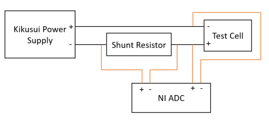
Figure S1: Wiring diagram for NLEIS data collection experiments.

S4.1 NLEIS Data collection procedure

NLEIS data, in the form of time-domain voltage and current sinusoids, was collected using the following set of procedures:

1. The cell was placed in a thermal chamber (Vötsch VT 4002) at $19\text{\,}\mathrm{\SIUnitSymbolCelsius}$ and initially left for 90 minutes to reach thermal equilibrium.

2. Thermal limits were checked, as per Section S4.2.

3. The following steps were executed at each DoD, starting at 10% DoD and ending at 90% DoD, at intervals of 10%:

   1. NLEIS data was measured

   2. The cell was discharged by 10% DoD using constant $500\text{\,}\mathrm{m}\mathrm{A}$ current

   3. The cell was rested for 10 minutes.

To ensure a complete dataset, data recording was started before current excitation began and ended after the current excitation was stopped. This left each recorded data instance as shown in Fig. S2.

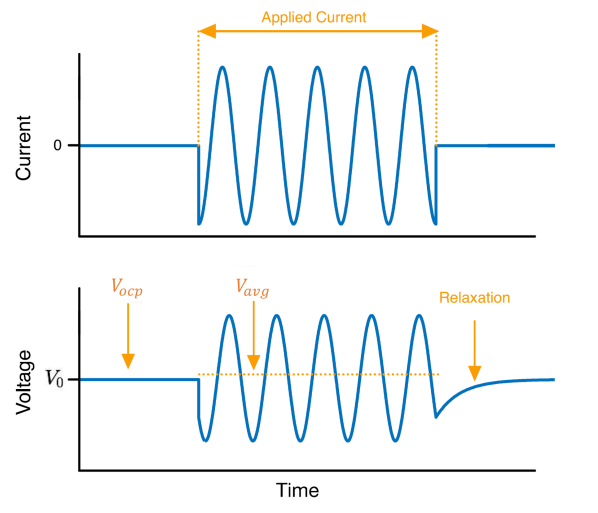
Figure S2: Exemplary current and voltage NLEIS measurement instance include non-excitation periods at the beginning and end

The extra measurement information either side of the perturbation facilitated capturing the OCV of the cell before each test, the average voltage of the cell under load, and the relaxation period after the load was removed.

S4.2 Thermal limits

A type-T nickel-copper-constantin thermocouple was attached to the surface of the pouch cell with tape and connected to a National Instruments (NI) 9213 temperature input module. The thermocouple was used firstly as a safety check to stop the experiment in the event of overheating, and secondly to augment the current and voltage data with time dependant temperature data.

Before each measurement, thermal limits were checked, and testing was stopped if these were exceeded. Specifically, the temperature before and after any measurement had to be less than $25\text{\,}\mathrm{\SIUnitSymbolCelsius}$, and the difference between the beginning and end temperatures had to be less than $2\text{\,}\mathrm{\SIUnitSymbolCelsius}$.

S4.3 Control and data acquisition

The power supply/load (Kikusui PBZ60-6.7) was externally controlled from a computer (Windows, Intel Core i9-9800HK $32\text{\,}\mathrm{G}\mathrm{B}$ RAM and $1\text{\,}\mathrm{T}\mathrm{B}$ RAID 5 storage). The data acquisition system (NI 9239 ADC module, 9213 temperature input module, and cDAQ-9188 back-plane) was also connected to the same computer, and a MATLAB script was written to control the system and measure data at $24\text{\,}\mathrm{b}\mathrm{i}\mathrm{t}\mathrm{s}$ and $50\text{\,}\mathrm{k}\mathrm{H}\mathrm{z}$, including careful consideration of memory issues due to the lengthy duration of the tests.

S4.4 Data processing

The measurements were stored in a database spanning 8 DoDs and 61 frequencies for each experimental campaign. For processing, first each dataset was trimmed to leave just sinusoids. This was done by locating the first peak in the current signal following the rising edge, then iterating the following steps until all other peaks were found:

1. The first current value within 99% of the expected peak current was established and marked as the start of the clipped signal. Failing this, the search was attempted again with decreasing accuracy levels: 1%, 5%, 15%, 25%, or notified an error.

2. The expected number of samples to the next peak was calculated by dividing the sampling frequency by the test excitation frequency.

3. If another peak was then found, the algorithm went back to step 2). Otherwise the last available peak was marked as the end of the clipped signal.

The DC component of voltage was removed by taking the average voltage under load and subtracting this from the measured voltages. To quantify the harmonics the voltage and current signals were multiplied by a Hann window function then Fourier transformed.

S4.5 OCP Functions and electrode balancing

Three-electrode data for the Kokam SLPB533459H4 cell from McTurk et al. [3] gives $U_{\pm}^{*}$ as a function of discharge capacity $Q^{*}$, which we converted to normalised discharge capacity $Q=Q^{*}/Q_{\mathrm{cap}}^{*}=\text{DoD}/100$ where $Q_{\mathrm{cap}}^{*}=$ $749\text{\,}\mathrm{m}\mathrm{A}\mathrm{h}$. Analytical expressions were fitted to this data using the nonlinear least squares minimiser lsqnonlin in MATLAB, giving

$$U_{-}^{*}= \,\,0.9577+\frac{0.0575Q-0.0533Q^{2}}{1-0.9877Q^{2}}-0.0760\tanh[25.6264(Q-0.9063)]$$

$$+0.0171\tanh[18.2444(Q-0.6530)]-0.0051\tanh[7.8242(Q-0.5474)]$$

$$+0.9226\tanh[9.3014(Q-1.0513)]+0.0127\tanh[34.6668(Q-0.2353)],$$ (S4.1)

and

$$U_{+}^{*}= \,\,9.8219-0.9241Q-5.3099\tanh[8.7293(Q+0.3418)]$$

$$-0.7503\tanh[6.2419(Q-0.7826)]+1.6105\tanh[3.8390(Q-0.8676)]$$

$$-0.5861\tanh[6.7659(Q-0.9774)]-0.2770\tanh[0.0109(Q-0.5488)],$$ (S4.2)

with fit RSMEs of $5.3\text{\,}\mathrm{m}\mathrm{V}$ and $6.4\text{\,}\mathrm{m}\mathrm{V}$, respectively. These are shown in the paper in Figs. LABEL:fig:kokam_OCPs($a$)-($b$).

The stoichiometry limits $c_{\pm}^{0\%}$ and $c_{\pm}^{100\%}$, corresponding to 0% and 100% DoD ($Q=0$ and 1), were chosen using knowledge of the electrode chemistries. In the negative electrode, which is graphite, they were chosen so that the staging between the different phases (indicated by the peaks in $\mathrm{d}U_{-}^{*}/\mathrm{d}Q$) occurs in the expected ranges. In particular, choosing the centre of the first and second visible peaks (Stages 2 and 3) to be at $c_{-}=0.5$ and $c_{-}=0.24$, results in $c_{-}^{0\%}=0.66$, $c_{-}^{100\%}=0.01$. The positive electrode consists of NMC, but the precise mixture of materials has not been characterised for these cells to our knowledge. Thus we chose stoichiometry limits $c_{+}^{0\%}=0.4$, $c_{+}^{100\%}=1$, typical for similar cells from the same manufacturer [4, 5]. At these values, the capacity parameter values $\xi_{\pm}$ follow from (LABEL:eq:ksi_stoichiometry_relation), giving $\xi_{-}=8.13\times 10^{-5}$, $\xi_{+}=7.41\times 10^{-5}$. The OCPs can then also be expressed as functions of $c_{\pm}$ directly by substituting $Q=(c_{\pm}-c_{\pm}^{0\%})(c_{\pm}^{100\%}-c_{\pm}^{0\%})$ into (S4.1)-(S4.2).

Derivatives with respect to $c_{\pm}$ may be calculated using the chain rule,

$$U_{\pm}^{*\prime}(c_{\pm}) =\frac{\mathrm{d}U_{\pm}^{*}}{\mathrm{d}c_{\pm}}=\frac{1}{c_{\pm}^{100\%}-c_{\pm}^{0\%}}\frac{\mathrm{d}U_{\pm}^{*}}{\mathrm{d}Q}.$$ (S4.3)

The second derivatives, however, are not captured sufficiently well by the expressions (S4.1)-(S4.2), which is clear from looking at the slope of $\mathrm{d}U_{+}^{*}/\mathrm{d}Q$ in Fig. LABEL:fig:kokam_OCPs. Hence, in the results section, when calculation of the second derivatives was necessary, we did this directly from the data using second-order central differences.

S5 Further parameter estimation details

S5.1 Maximum likelihood estimation (MLE)

Assuming the voltage harmonic data is normally distributed around the model predictions, as in (LABEL:eq:synthetic-data-noise) of the paper, with residuals on the real and imaginary components of the $n$-th harmonic distributed as $\varepsilon_{n,r},\varepsilon_{n,i}\sim N(0,\sigma_{n}^{*2})$, the joint probability distribution of the observations $\widehat{V}_{1,j}^{*,\mathrm{data}},\widehat{V}_{2,j}^{*,\mathrm{data}}$ across the set of frequencies $\omega_{j},j=1,2,\ldots,N_{\omega}$ is given by

$$p(\widehat{V}_{1,j}^{*,\mathrm{data}},\widehat{V}_{2,j}^{*,\mathrm{data}}|\omega_{i},\bm{\theta},\sigma_{n}^{*})= \prod_{n=1}^{2}\prod_{j=1}^{N_{\omega}}(\sqrt{2\pi\sigma_{n}^{*2}})^{-2}\exp\left(-\frac{1}{2\sigma_{n}^{*2}}\left|\widehat{V}_{n}^{*}(\omega_{j};\bm{\theta})-\widehat{V}_{n,j}^{*,\mathrm{data}}\right|^{2}\right)$$ (S5.1)

which is also the likelihood $L(\bm{\theta},\sigma_{1}^{*},\sigma_{2}^{*})$ of the parameters $\bm{\theta},\sigma_{1}^{*},\sigma_{2}^{*}$ given the data. Maximising $L$ over $\bm{\theta},\sigma_{1}^{*},\sigma_{2}^{*}$ then gives a maximum likelihood estimator. Equivalently, we may minimise the negative log-likelihood, $-\log L$, which is (substituting $\widehat{V}_{n}^{*}=(\hat{I}^{*})^{n}Z_{n}^{*}$):

$$-\log L(\bm{\theta},\sigma_{1}^{*},\sigma_{2}^{*})= \,\,2N_{\omega}\log(2\pi\sigma_{1}^{*2})+2N_{\omega}\log(2\pi\sigma_{2}^{*2})$$

$$+\sum_{j=1}^{N_{\omega}}\left[\frac{|\hat{I}^{*}|^{2}}{2\sigma_{1}^{*2}}\left|Z_{1}^{*(1)}(\omega_{j};\bm{\theta})-Z_{1,j}^{*,\mathrm{data}}\right|^{2}+\frac{|\hat{I}^{*}|^{4}}{2\sigma_{2}^{*2}}\left|Z_{2}^{*(2)}(\omega_{j};\bm{\theta})-Z_{2,j}^{*,\mathrm{data}}\right|^{2}\right].$$ (S5.2)

Minimizing over each $\sigma_{n}^{*}$, by setting $\partial(-\log L)/\partial\sigma_{n}^{*}=0$ and rearranging for $\sigma_{n}^{*}$, gives

$$\sigma_{n}^{*2} =\frac{|\hat{I}^{*}|^{2n}}{2N_{\omega}}\sum_{j=1}^{N_{\omega}}\left|Z_{n}^{*(n)}(\omega_{j};\bm{\theta})-Z_{n,j}^{*,\mathrm{data}}\right|^{2},\qquad n=1,2,$$ (S5.3)

which can be used to eliminate the $\sigma_{n}^{*}$ in (S5.2), leaving

$$-\log L(\bm{\theta})= \,\,2N_{\omega}\left[l_{1}(\bm{\theta})+l_{2}(\bm{\theta})+\log\left(\frac{\pi|\hat{I}^{*}|^{2}}{N_{\omega}}\right)+\log\left(\frac{\pi|\hat{I}^{*}|^{4}}{N_{\omega}}\right)+1\right].$$ (S5.4)

where

$$l_{1}(\bm{\theta}) =\log\left(\sum_{j=1}^{N_{\omega}}\left|Z_{1}^{*(1)}(\omega_{j};\bm{\theta})-Z_{1,j}^{*,\mathrm{data}}\right|^{2}\right),$$ (S5.5)

$$l_{2}(\bm{\theta}) =\log\left(\sum_{j=1}^{N_{\omega}}\left|Z_{2}^{*(2)}(\omega_{j};\bm{\theta})-Z_{2,j}^{*,\mathrm{data}}\right|^{2}\right),$$ (S5.6)

Therefore, the MLE problem for $\bm{\theta}$ is reduced to

$$\hat{\bm{\theta}}_{\mathrm{NLEIS}} =\underset{\bm{\theta}}{\mathrm{argmin}}\,(l_{1}(\bm{\theta})+l_{2}(\bm{\theta})).$$ (S5.7)

with total log-likelihood $l_{12}(\bm{\theta})=l_{1}+l_{2}$.

S5.2 Numerical optimization

The minimization problems above were solved using nonlinear optimization routines in MATLAB employing bound constraints. When using synthetic data, a local gradient-based minimizer fmincon was used, initialised at the true parameter values (except for $\beta_{\pm}$ when using EIS data—see the Results section. This allowed efficient and robust convergence to the known global minimum. We employed the SQP algorithm with optimality, constraint, and step size tolerances of $10^{-7}$, $10^{-10}$, and $10^{-12}$. The objective function may have several local minima thus, when using experimental data where the true global minimum is unknown, we used a global minimizer GlobalSearch which starts the aforementioned local solver (fmincon) at multiple start points (which we set to 300) generated with a scatter search algorithm within the parameter bounds, identifying basins of attraction. In all cases, the chosen parameter bounds were $\chi_{\pm},C_{\pm}\in[0,10]$, $\beta_{\pm}\in[0,1]$, $\tau_{\mathrm{d},\pm}\in[0,10^{7}]$, unless otherwise specified.

S6 Large separation of timescales

In this section, we compare the exact impedance expressions (LABEL:eq:Z11_pm), (LABEL:eq:Z22_pm) and (LABEL:eq:Z02_pm) to the simplified (composite) expressions (LABEL:eq:Z11_pm_comp), (LABEL:eq:Z22_pm_comp) and (LABEL:eq:Z02_pm_comp) which assume that the capacitive timescale $R_{\pm}^{(0)}C_{\pm}$ is much shorter than the diffusive one $\tau_{\mathrm{d},\pm}=1/D_{\pm}^{(0)}$. Fig. S3 shows the full-cell impedances as calculated from both sets of expressions—for the parameters in Tables S1-S2, and when the nondimensional capacitances $C_{\pm}$ are increased. The simplified formulae were derived assuming $C_{\pm}R_{\pm}^{(0)}/\tau_{\mathrm{d},\pm}\ll 1$, and for the base case here (blue lines), these ratios are $O(10^{-4})$, $O(10^{-6})$ for the positive and negative electrodes, respectively. The well-separated timescales assumption is clearly satisfied, and thus the composite expressions agree excellently with the full expression for all frequencies. Indeed, excellent agreement is observed even when $C_{\pm}$ values (and hence the capacitance timescales) are increased by up to 2 orders of magnitude. As $C_{\pm}$ values are increased, the composite expression should first breakdown for frequencies in the “overlap region” (see (LABEL:eq:omega_overlap)), where still only small discrepancies are observed. The mean relative errors (mean absolute error scaled by the maximum magnitude of the exact impedance), defined as

$$\mbox{MRE}_{n,m} =\frac{\frac{1}{N_{\omega}}\sum_{\omega}|Z_{n}^{(m),\mathrm{comp}}(\omega)-Z_{n}^{(m)}(\omega)|}{\max_{\omega}|Z_{n}^{(m)}(\omega)|},$$ (S6.1)

were found to be 0.03%, 0.64%, 0.04% for $Z_{1}^{(1)}$, $Z_{2}^{(2)}$, $Z_{0}^{(2)}$ at the original values of $C_{\pm}$, and still only 0.39%, 1.69%, 0.45% at the largest values of $C_{\pm}$.

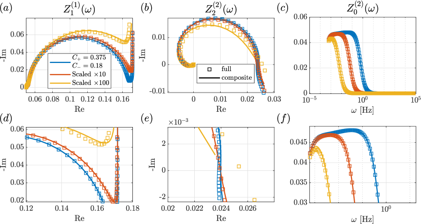
Figure S3: Comparison of impedance formulae for $Z_{1}^{(1)}$, $Z_{2}^{(2)}$, and $Z_{0}^{(2)}$. The full formula (squares) uses (LABEL:eq:Z11_pm)-(LABEL:eq:Z02_pm), and composite formula uses (LABEL:eq:Z11_pm_comp)-(LABEL:eq:Z02_pm_comp), for parameters in Table S1 at $\mathrm{DoD}=50\%$. Bottom panels zoom into the “overlap region” in the panels above. Frequency range $10^{-4}\leq\omega/2\pi\leq 10^{4}$ Hz. The different colours are for increasing values of the capacitances $C_{\pm}$, i.e. scaled by 10 (red) and 100 (yellow).

References

• [1] M. D. Murbach, V. W. Hu, D. T. Schwartz, Nonlinear electrochemical impedance spectroscopy of lithium-ion batteries: Experimental approach, analysis, and initial findings, Journal of The Electrochemical Society 165 (11) (2018) A2758–A2765. doi:10.1149/2.0711811jes.
• [2] S. G. Marquis, V. Sulzer, R. Timms, C. P. Please, S. J. Chapman, An asymptotic derivation of a single particle model with electrolyte, Journal of The Electrochemical Society 166 (15) (2019) A3693. doi:10.1149/2.0341915jes.
• [3] E. McTurk, C. R. Birkl, M. R. Roberts, D. A. Howey, P. G. Bruce, Minimally invasive insertion of reference electrodes into commercial lithium-ion pouch cells, ECS Electrochemistry Letters 4 (12) (2015) A145–A147. doi:10.1149/2.0081512eel.
• [4] M. Ecker, T. K. D. Tran, P. Dechent, S. Käbitz, A. Warnecke, D. U. Sauer, Parameterization of a physico-chemical model of a lithium-ion battery: I. Determination of parameters, Journal of The Electrochemical Society 162 (9) (2015) A1836–A1848. doi:10.1149/2.0551509jes.
• [5] M. Ecker, S. Käbitz, I. Laresgoiti, D. U. Sauer, Parameterization of a physico-chemical model of a lithium-ion battery: II. Model validation, Journal of The Electrochemical Society 162 (9) (2015) A1849–A1857. doi:10.1149/2.0541509jes.