emgr – EMpirical GRamian Framework
Version 5.99
Software Release Paper

Abstract

Version 5.99 of the empirical Gramian framework – emgr – completes a development cycle which focused on parametric model order reduction of gas network models while preserving compatibility to the previous development for the application of combined state and parameter reduction for neuroscience network models. Secondarily, new features concerning empirical Gramian types, perturbation design, and trajectory post-processing, as well as a Python version in addition to the default MATLAB / Octave implementation, have been added. This work summarizes these changes, particularly since emgr version 5.4, see Himpe, 2018 [Algorithms 11(7): 91], and gives recent as well as future applications, such as parameter identification in systems biology, based on the current feature set.

Keywords: Control Theory, System Theory, Nonlinear Systems, System Gramians, Empirical Gramians

1 Project History and Overview

The empirical Gramian framework (emgr) is an open-source MATLAB (and Octave-compatible) software package for the computation of empirical system Gramians and empirical covariance matrices, which are (approximations to the) essential operators in (nonlinear) system theory.

Originally, emgr was started to provide reusable computational kernels with a unified interface, while the interface is inspired by the gram function of the Control System Toolbox [MathWorks, nd] and the “Nonlinear Model Reduction Routines” [Sun and Hahn, nd].

The first release (version 0.9) coincided with the “MoRePaS 2” workshop in 2012, while a first summary of the capabilities is published in [Himpe and Ohlberger, 2013] (based on version 1.3), and detailed descriptions of emgr are given in [Himpe, 2017] (based on version 3.9) and [Himpe, 2018] (based on version 5.4). Marking the ten-year anniversary of emgr’s development, version 5.99 [Himpe, 2022] was released. And relative to version 5.4, various major features have been added, which this work summarizes.

The (empirical) system Gramian matrices have a multitude of system theoretic applications, which include model reduction, parameter identification, control configuration selection, sensitivity analysis, optimal placement, nonlinearity quantification, or system characterization via indices and invariants. Beyond system and control theory, areas such as uncertainty quantification use numerically approximations of operators which are computable as empirical Gramians, for example Hessians [Lieberman et al., 2013]. Recent interesting uses for system Gramians in particular applications are: pose detection [Avant and Morganson, 2019], traffic networks [Bianchin and Pasqualetti, 2020], tau functions [Blower and Newsham, 2021], and vulnerability analysis [Babazadeh, 2022].

2 New Features

A detailed description of the features up to and including emgr 5.4 is given in [Himpe, 2018]. This section summarizes the major new features implemented since version 5.4 onwards until the latest version 5.99. These features are grouped in to five categories: Gramian variants, input functions, trajectory weighting, parameter identifiability, and Python version.

2.1 Gramian Variants

emgr provides seven empirical Gramians: controllability, observability, cross, linear cross, sensitivity, identifiability and joint Gramian. Of those, only the cross-Gramian derived empirical Gramians (cross, linear cross and joint Gramian) used to provide a variant, specifically for non-square or non-symmetric systems [Himpe, 2018, Sec. 3.1.5]. Over the recent releases, variants also for the controllability- and observability-based Gramians were added.

It is noted here, that the loadability Gramian from [Tolks and Ament, 2017] is not a system Gramian but a standard Gram matrix [Wikipedia contributors, 2022], and hence does not need to be computed via emgr.

2.1.1 Output Controllability Gramian

The output reachability Gramian, or more generally the output controllability Gramian [Kreindler and Sarachik, 1964], encodes the controllability of the output $y:\operatorname{\mathbb{R}}\to\operatorname{\mathbb{R}}^{Q}$ instead of the controllability of the state $x:\operatorname{\mathbb{R}}\to\operatorname{\mathbb{R}}^{N}$. It has various applications in system theory, for example in control configuration selection [Halvarsson, 2008], while more recently the empirical output-controllability covariance matrix (EOCCM) [Méndez-Blanco and Özkan, 2021] is employed for parameter identifiability. An empirical output controllability Gramian can always be computed via the empirical controllability Gramian, given a linear output operator $C$ of the underlying system,

$$\widehat{W}_{OC}=C\widehat{W}_{C}C^{\intercal}.$$

However in version 5.8, direct computation of the output controllability Gramian was included; not only to provide a more memory efficient computation for large-scale systems by computing an empirical output controllability Gramian from output trajectory data directly, instead of state trajectories, but also to approximate the output controllability for systems with nonlinear output operators. Following the format of [Himpe, 2018], it is defined as:

Definition 1 (Empirical Output Controllability Gramian)

Given non-empty sets $E_{u}$ and $S_{u}$, the empirical output controllability Gramian $\widehat{W}_{OC}\in\operatorname{\mathbb{R}}^{Q\times Q}$ is defined as:

$$\widehat{W}_{OC} :=\frac{1}{|S_{u}|}\sum_{k=1}^{|S_{u}|}\sum_{m=1}^{M}\frac{1}{c_{k}^{2}}\int_{0}^{T}\Psi^{km}(t)\operatorname{\mathrm{d}\!}t$$

$$\Psi^{km}(t) =(y^{km}(t)-\bar{y}^{km})(y^{km}(t)-\bar{y}^{km})^{\intercal}\in\operatorname{\mathbb{R}}^{Q\times Q},$$

with the output trajectories $y^{km}(t)\in\operatorname{\mathbb{R}}^{Q}$ for the input configurations $\hat{u}^{km}(t)=c_{k}e^{m}\circ u(t)+\bar{u}$, $c_{k}\in S_{u}$, $e_{m}\in E_{u}$, and offsets $\bar{u}\in\operatorname{\mathbb{R}}^{M}$, $\bar{x}^{km}\in\operatorname{\mathbb{R}}^{N}$.

2.1.2 Average Observability Gramian

An idea similar to the non-symmetric (empirical) cross Gramian [Himpe, 2018, Sec. 3.1.5], is an average observability Gramian, which is hinted at in [Rong and Michael, 2016]. Practically, this means for multiple output systems, that all outputs are summed up yielding a single (average) output. This variant, added in version 5.7, also extends to the augmented empirical observability Gramian, and thus the empirical identifiability Gramian.

The empirical local observability Gramian [Krener and Ide, 2009], could have been a potential variant, yet, [Rong and Michael, 2016, Sec. II.A] illustrates why the standard empirical observability Gramian suffices.

2.2 Input Functions

Already up to version 5.4, emgr provided means to pass a custom function of a single (time) argument as input function for the empirical Gramian computation or select from the included default input functions: impulse, decaying chirp, or pseudo-random binary sequence. Subsequently, two more default input functions were implemented:

2.2.1 Step Function Input

Since for (semi-discrete) hyperbolic partial differential equation models, with inputs and outputs at the boundaries, step functions are a relevant training input, which was demonstrated heuristically in [Grundel et al., 2019], in version 5.7 a constant “step” function was added as default input function:

$$u_{\text{step}}(t):=1.$$

This training input became the default for data-driven reduced order gas network models in the morgen platform [Himpe et al., 2021], which utilizes emgr as model reduction back-end.

2.2.2 Sine Cardinale Input

A smooth alternative to impulse input is a sine cardinale (sinc) input, as it was employed in [Arjona et al., 2011]. In version 5.8, a scaled $\operatorname{sinc}$ input function has been included into the set of default inputs:

$$u_{\text{sinc}}(t):=\begin{cases}\frac{\sin(th^{-1})}{th^{-1}}&t\neq 0,\\ \leavevmode\nobreak\ \leavevmode\nobreak\ \leavevmode\nobreak\ \leavevmode\nobreak\ \leavevmode\nobreak\ 1&t=0,\end{cases}$$

for time-step width $h>0$.

2.3 Trajectory Weighting

As mentioned in [Himpe, 2018, Sec. 5.3] trajectory weighting, could be implemented by using the custom inner product interface. However, a set of weighting functions has been included, originally motivated by time domain weighting. Nonetheless, trajectory independent weightings like in [Mitra, 1969] are still achieved via the inner product interface.

2.3.1 Time-Weighting

Time-domain weighting of Gramians was initially proposed in [Schelfhout and De Moor, 1995], particularly, using monomials of the time variable, and also provides an error bound [Sreeram, 2002] if used in conjunction with balanced truncation [Breiten and Stykel, 2021]. In version 5.8, linear and a quadratic time-domain weighting was included, based on a time-weighted linear system Gramian and [Himpe, 2018, Sec. 3.1]:

$$W_{*} =\frac{1}{r!}\int_{0}^{\infty}t^{r}\operatorname{e}^{A_{1}x(t)}D\operatorname{e}^{A_{2}x(t)}\operatorname{\mathrm{d}\!}t$$

$$\to\widehat{W}_{*} =\frac{1}{\dots}\sum\dots\sum\frac{1}{\dots}\;\frac{1}{r!}\int t^{r}\;\Psi(t)\operatorname{\mathrm{d}\!}t$$

for $r\in\{1,2\}$ and all computable empirical Gramians. Practically, such time-weighting emphasizes “later” parts of a simulated trajectory in the empirical Gramian, over the “earlier” parts, like the initial state / output. Note, that the scaling factor $\frac{1}{r!}$ from [Sreeram, 2002] is included for convenience, in case for a typical use in conjunction with balanced truncation.

2.3.2 Reciprocal Time-Weighting

Furthermore, in the latest version 5.99 a time-reciprocal weighting, also based on a weighted linear system Gramian and [Himpe, 2018, Sec. 3.1]:

$$W_{*} =\int_{0}^{\infty}\frac{1}{\sqrt{\pi t}}\operatorname{e}^{A_{1}x(t)}D\operatorname{e}^{A_{2}x(t)}\operatorname{\mathrm{d}\!}t$$

$$\to\widehat{W}_{*} =\frac{1}{\dots}\sum\dots\sum\frac{1}{\dots}\int\;\frac{1}{\sqrt{\pi t}}\Psi(t)\operatorname{\mathrm{d}\!}t$$

following [Glover, 1987, Sec. 3.2] was included, i.e. to allow numerical verification of the lower error bound presented in there, and to provide a time-weighting emphasizing “earlier” parts of a simulated trajectory, in contrast to the typical time-weighting. Note, that practically at time $t=0$ the scaling factor is set to $\sqrt{\frac{2}{\pi\Delta t}}$, which was determined heuristically to be suitable.

2.3.3 Column-Based Weighting

The column-based weighting originates in an approach to suboptimal control from [Hyun et al., 2017, Def. 2], and defines a weighted Gramian which normalizes the state $x$ (or output $y$) at each time instance by its length, i.e.:

$$\hat{x}(t) :=x(t)\cdot\|x(t)\|_{2}^{-1},$$

$$\hat{y}(t) :=y(t)\cdot\|y(t)\|_{2}^{-1}.$$

2.3.4 Row-Based Weighting

The row-based weighting is based on component-wise scale normalization. This means each component $i$ of the utilized state $x$ or output $y$ trajectories for the Gramians is normalized by its (absolute) maximum value, i.e.:

$$\hat{y}_{i}(t) :=x_{i}(t)\cdot\|x_{i}\|_{\infty}^{-1},$$

$$\hat{y}_{i}(t) :=y_{i}(t)\cdot\|y_{i}\|_{\infty}^{-1},$$

which means all component (output) trajectories evolve in the interval $[-1,1]$.

2.4 Parameter Identifiability

More recently parameter identification of nonlinear systems with low-dimensional state-space, but high-dimensional parameter-space became a use-case for emgr, [Falkenhagen et al., 2022]. This motivated the following enhancements:

2.4.1 Schur Complement

Initially, parameter identification was the basis for the combined state and parameter reduction [Himpe, 2017] of nonlinear systems with high-dimensional state and parameter spaces, but homogeneous parameters, hence the matrix-inverse inside the Schur complement is only roughly approximated by a truncated Neumann series.

To improve accuracy of the empirical (cross-)identifiability Gramian, a more accurate Schur complement option was added in version 5.99, which computes the inner inverse as Moore-Penrose pseudo-inverse:

$$W_{I,\text{exact}} =W_{P}-W_{M}^{\intercal}W_{O}^{+}W_{M},$$

$$W_{\ddot{I},\text{exact}} =-\frac{1}{2}W_{m}^{\intercal}(W_{X}+W_{X}^{\intercal})^{+}W_{m}.$$

2.4.2 Parameter Centering

Originally parameter-related Gramians (empirical sensitivity, identifiability, joint Gramian) required a minimum and maximum parameter to define the range of perturbation. Recently in version 5.99, a mode was added, which requires minimum, maximum and nominal parameter, which then sets up a range of perturbation with respect to the nominal value instead of the minimum or (logarithmic) mean.

2.5 Python Version

Since version 5.6, a Python (version 3) variant of emgr is also maintained, that provides the same features, and closely resembles the MATLAB interface and function signature. The elaborate testing, prototype and wrapper code, as for the MATLAB variant, is not available yet. However, a combinatorial testing of configurations is supported.

3 Application Demonstration

A current application for emgr’s empirical Gramians is, after combined state and parameter reduction for brain connectivity inference [Himpe, 2017], and parametric model order reduction for gas networks [Himpe et al., 2021], parameter identification for systems biology models.

Such application is exemplarily demonstrated on a benchmark model – the IL13-Induced JAK/STAT signaling model from [Raue et al., 2014], which is also tested in [Villaverde et al., 2016] and [Stigter and Joubert, 2021]. This model has $\dim(u(t))=1$ input, $\dim(x(t))=10$ states, $\dim(y(t))=8$ outputs and $\dim(\theta)=23$ parameters, and the following nonlinear vector field as well as linear output function (in simplified form):

$$\dot{x}(t) =\begin{bmatrix}\theta_{6}x_{2}(t)-\theta_{5}x_{1}-c_{1}\theta_{1}x_{1}(t)u_{1}(t)\\ \theta_{5}x_{1}(t)-\theta_{6}x_{2}(t)\\ \theta_{2}x_{3}(t)(x_{6}(t)-c_{3})+c_{1}\theta_{1}x_{1}(t)u_{1}(t)\\ -\theta_{3}x_{4}(t)-\theta_{2}x_{3}(t)(x_{6}(t)-c_{3})\\ \theta_{3}x_{4}(t)-\theta_{4}x_{5}(t)\\ -c_{2}\,\theta_{8}(x_{6}(t)-c_{3})-\frac{\theta_{7}x_{3}(t)x_{6}(t)}{\theta_{13}x_{1}(t)+1}-\frac{\theta_{7}x_{4}(t)x_{6}(t)}{\theta_{13}x_{1}(t)+1}\\ \theta_{9}x_{7}(t)(x_{6}(t)-c_{3})-c_{2}x_{10}(t)(x_{7}(t)-c_{4})\\ -\theta_{11}(x_{7}(t)-c_{4})\\ -c_{1}\theta_{12}x_{9}(t)u_{1}(t)\\ \frac{\theta_{14}x_{8}(t)}{\theta_{15}+x_{8}(t)}-\theta_{16}x_{10}(t)\end{bmatrix},$$

$$y(t) =\begin{bmatrix}x_{1}(t)+x_{3}(t)+x_{4}(t)\\ \theta_{18}(x_{3}(t)+x_{4}(t)+x_{5}(t)+c_{5}-x_{9})\\ \theta_{19}(x_{4}(t)+x_{5}(t))\\ \theta_{20}(c_{3}-x_{6}(t))\\ \theta_{21}x_{8}(t)\\ \theta_{17}\theta_{22}\theta_{11}^{-1}x_{8}(t)\\ x_{10}(t)\\ c_{4}-x_{7}(t)\end{bmatrix},$$

with constants $c_{1}=2.265$, $c_{2}=91$, $c_{3}=2.8$, $c_{4}=165$, and $c_{5}=0.34$. Additionally, the initial state has a parameter dependency:

$$x_{0}=\begin{bmatrix}1.3&\theta_{23}&0&0&0&c_{3}&c_{4}&0&c_{5}&0\end{bmatrix}^{\intercal}.$$

As initial-state-parameters are not supported by default in emgr, but can be emulated by providing a solver wrapper[Himpe, 2018, Sec. 5.5] which sets the parameter in the initial states and passes the updated initial state to the actual solver.

To assess the parameter identifiability, the empirical identifiability Gramian is computed via the augmented empirical observability Gramian, of which its singular value decomposition $W_{I}=U\Sigma U^{\intercal}$ is analyzed. This numerical experiment is conducted in MATLAB 2022a on a AMD Ryzen 5 4500U with 16GiB RAM.

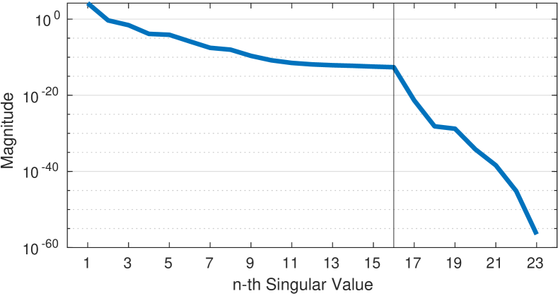
Figure 1: Singular values of the empirical identifiability Gramian for the JAK/STAT benchmark system’s parameters.

The singular values $\Sigma_{ii}$ are plotted in Fig. 1 and indicate that the singular vectors, associated to the seven smallest singular values, $\{u_{17},\dots,u_{23}\}$ contain linear combinations of the original parameters that are least identifiable. To reconstruct the contributions of those, these singular vectors are summed after taking their element-wise absolute value, $\bar{u}_{2}:=\sum_{k=17}^{23}|u_{k}|$, which yields the overall contribution of original parameter fractions to the “unidentifiable” singular vectors. The dominant contribution is given by the five structurally unidentifiable parameters $\{\theta_{11},\theta_{15},\theta_{17},\theta_{21},\theta_{22}\}$, as well as by the practically unidentifiable parameters $\{\theta_{4},\theta_{14},\theta_{16},\theta_{19}\}$. The remaining practically unidentifiable parameters $\{\theta_{3},\theta_{12}\}$ are not contributing. However, all structurally unidentifiable parameters are located, and particularly, all identifiable parameters do not contribute (the respective elements of $\bar{u}_{2}$ have relative magnitudes below $10^{-7}$) to the singular vectors of small singular values. Thus, the results of the empirical-Gramian-based parameter identification agrees with other studies on this system in terms structural identifiability. Furthermore, the matrix of singular vectors associated to the dominant singular values, represents a lower-dimensional reparametrization of the system.

4 Summary

In a decade of research in empirical system Gramians and working on emgr, I conclude that an empirical-Gramian-based approach typically gives an acceptable approximate answer, no matter the system’s complexities, which makes this data-driven mathematical technology a somewhat universal tool for linear and nonlinear control and system-theory and engineering. Lastly, I note that more information and documentation on emgr can be found on:

https://gramian.de

Code Availability

The source code of the numerical experiments is licensed under BSD-2-Clause License, can be obtained from:

doi:10.5281/zenodo.7048585

and is authored by: C. Himpe.

References

- [Arjona et al., 2011] Arjona, M. A., Cisneros-Gonazález, M., and Hernández, C. (2011). Parameter estimation of a synchronous generator using a sine cardinal perturbation and mixed stochastic-deterministic algorithms. IEEE Transactions on Industrial Electronics, 58(2):486–493.
- [Avant and Morganson, 2019] Avant, T. and Morganson, K. A. (2019). Observability properties of object pose estimation. In Proceedings of the American Control Conference, pages 5134–5140.
- [Babazadeh, 2022] Babazadeh, M. (2022). Gramian-based vulnerability analysis of dynamic networks. IET Control Theory & Application, 16(6):625–637.
- [Bianchin and Pasqualetti, 2020] Bianchin, G. and Pasqualetti, F. (2020). Gramian-based optimization for the analysis and control of traffic networks. IEEE Transactions on Intelligent Transportation Systems, 21(7):3013–3024.
- [Blower and Newsham, 2021] Blower, G. and Newsham, S. L. (2021). Tau functions associated with linear systems. In Operator Theory, Functional Analysis and Applications, pages 63–94.
- [Breiten and Stykel, 2021] Breiten, T. and Stykel, T. (2021). Balancing-related model reduction methods. In Benner, P., Grivet-Talocia, S., Quarteroni, A., Rozza, G., Schilders, W., and Silveira, L. M., editors, System- and Data-Driven Methods and Algorithms, volume 1 of Model Order Reduction, chapter 2, pages 15–56. De Gruyter.
- [Falkenhagen et al., 2022] Falkenhagen, U., Himpe, C., Kloft, C., Knoechel, J., and Huisinga, W. (2022). Sample-based robust model order reduction for nonlinear systems biology models. In In Preparation.
- [Glover, 1987] Glover, K. (1987). Model reduction: A tutorial on Hankel-norm methods and lower bounds on errors. IFAC Proceedings Volume (10th Triennial IFAC Congress on Automatic Control), 20(5):293–298.
- [Grundel et al., 2019] Grundel, S., Himpe, C., and Saak, J. (2019). On empirical system Gramians. Proc. Appl. Math. Mech., 19(1):e201900006.
- [Halvarsson, 2008] Halvarsson, B. (2008). Comparison of some Gramian based interaction measures. In 2008 IEEE Int Symposium on Computer-Aided Control System Design, pages 128–143.
- [Himpe, 2017] Himpe, C. (2017). Combined State and Parameter Reduction for Nonlinear Systems with an Application in Neuroscience. PhD thesis, Westfälische Wilhelms-Universität Münster. Sierke Verlag Göttingen, ISBN 9783868448818.
- [Himpe, 2018] Himpe, C. (2018). emgr – the Empirical Gramian Framework. Algorithms, 11(7):91.
- [Himpe, 2022] Himpe, C. (2022). emgr – EMpirical GRamian framework (version 5.99). https://gramian.de.
- [Himpe et al., 2021] Himpe, C., Grundel, S., and Benner, P. (2021). Model order reduction for gas and energy networks. Journal of Mathematics in Industry, 11:13.
- [Himpe and Ohlberger, 2013] Himpe, C. and Ohlberger, M. (2013). A unified software framework for empirical Gramians. J. Math., 2013:1–6.
- [Hyun et al., 2017] Hyun, N.-s. P., Murali, V., and Verriest, E. I. (2017). Minimum sensitivity analysis for accurate open-loop controllers in linear systems using weighted Gramians. In Proceedings of the IEEE 56th Annual Conference on Decision and Control, pages 114–119.
- [Kreindler and Sarachik, 1964] Kreindler, E. and Sarachik, P. E. (1964). On the concepts of controllability and observability of linear systems. IEEE Trans. Autom. Control, 9(2):129–136.
- [Krener and Ide, 2009] Krener, A. and Ide, K. (2009). Measures of unobservability. In Proceedings of the 48th IEEE Conference on Decision and Control, 2009 held jointly with the 2009 28th Chinese Control Conference, pages 6401–6406.
- [Lieberman et al., 2013] Lieberman, C. E., Fidkowski, K., Willcox, K., and Van Bloemen Waanders, B. (2013). Hessian-based model reduction: large-scale inversion and prediction. Int. J. Numer. Methods Fluids, 71(2):135–150.
- [MathWorks, nd] MathWorks (n.d.). Control System Toolbox.
- [Méndez-Blanco and Özkan, 2021] Méndez-Blanco, C. S. and Özkan, L. (2021). Local parameter identifiability of large-scale nonlinear models based on the output sensitivity covariance matrix. IFAC-PapersOnLine (16th IFAC Symposium on Advanced Control of Chemical Processes ADCHEM 2021), 54(3):415–420.
- [Mitra, 1969] Mitra, D. (1969). matrix and the geometry of model equivalence and reduction. Proceedings of the Institution of Electrical Engineers, 116(6):1101–1106.
- [Raue et al., 2014] Raue, A., Karlsson, J., Saccomani, M. P., and Jirstrand, M. (2014). Comparison of approaches for parameter identifiability analysis of biological systems. Bioinformatics, 30(10):1440–1448.
- [Rong and Michael, 2016] Rong, Z. and Michael, N. (2016). Detection and prediction of near-term state estimation degradation via online nonlinear observability analysis. In IEEE International Symposium on Safety, Security, and Rescue Robotics (SSRR), pages 28–33.
- [Schelfhout and De Moor, 1995] Schelfhout, G. and De Moor, B. (1995). Time-domain weighted balanced truncation. In 3rd European Control Conference, pages 1–4.
- [Sreeram, 2002] Sreeram, V. (2002). Frequency response error bounds for time-weighted balanced truncation. In Proceedings of the 41st IEEE Conference on Decision and Control, pages 3330–3331.
- [Stigter and Joubert, 2021] Stigter, J. D. and Joubert, D. (2021). Computing measures of identifiability, observability and controllability for a dynamic system model with the StrucID app. IFAC PapersOnLine (19th IFAC Symposium on System Identification), 54(7):138–143.
- [Sun and Hahn, nd] Sun, C. and Hahn, J. (n.d.). Nonlinear Model Reduction Routines for MATLAB.
- [Tolks and Ament, 2017] Tolks, C. and Ament, C. (2017). Model order reduction of glucose-insulin homeostasis using empirical Gramians and balanced truncation. IFAC-PapersOnline (Proceedings of the 20th IFAC World Congress), 50(1):14735–14740.
- [Villaverde et al., 2016] Villaverde, A. F., Barreiro, A., and Papachristodoulou, A. (2016). Structural identifiability of dynamic systems biology models. PLOS Computational Biology, 12(10):e1005153.
- [Wikipedia contributors, 2022] Wikipedia contributors (2022). Gram matrix — Wikipedia, the free encyclopedia. https://en.wikipedia.org/w/index.php?title=Gram_matrix&oldid=1093332712. [Online; accessed 23-August-2022].