T²LR-Net: An Unrolling Reconstruction Network Learning Transformed Tensor Low-Rank prior for Dynamic MR Imaging

Abstract

While the methods exploiting the tensor low-rank prior are booming in high-dimensional data processing and have obtained satisfying performance, their applications in dynamic magnetic resonance (MR) image reconstruction are limited. In this paper, we concentrate on the tensor singular value decomposition (t-SVD), which is based on the Fast Fourier Transform (FFT) and only provides the definite and limited tensor low-rank prior in the FFT domain, heavily reliant upon how closely the data and the FFT domain match up. By generalizing the FFT into an arbitrary unitary transformation of the transformed t-SVD and proposing the transformed tensor nuclear norm (TTNN), we introduce a flexible model based on TTNN with the ability to exploit the tensor low-rank prior of a transformed domain in a larger transformation space and elaborately design an iterative optimization algorithm based on the alternating direction method of multipliers (ADMM), which is further unrolled into a model-based deep unrolling reconstruction network to learn the transformed tensor low-rank prior (T²LR-Net). The convolutional neural network (CNN) is incorporated within the T²LR-Net to learn the best-matched transform from the dynamic MR image dataset. The unrolling reconstruction network also provides a new perspective on the low-rank prior utilization by exploiting the low-rank prior in the CNN-extracted feature domain. Experimental results on two cardiac cine MR datasets demonstrate that the proposed framework can provide improved recovery results compared with the state-of-the-art optimization-based and unrolling network-based methods.

Index Terms—  dynamic MR imaging, transformed tensor low-rank prior, unrolling network, t-SVD, tensor nuclear norm

1 Introduction

The low-rank tensor models [1] have been proposed lately as a successful alternative to the low-rank matrix methods for high-dimensional data/image processing. In particular, the tensor low-rank priors are constructed via tensor decomposition, e.g., the Canonical-Polyadic (CP) decomposition and the Tucker decomposition. However, the CP rank is generally NP-hard to compute, and the convex relaxation is intractable [1]; The TUCKER rank is a vector with each element being the rank of a certain unfolding matrix [1], the sum of the nuclear norms (SNN) of which is usually considered to constrain the low TUCKER rank. However, the SNN is not the convex envelope of the sum of TUCKER rank, which may be suboptimal in the applications [2].

In this paper, we concentrate on the tensor singular value decomposition (t-SVD) [3], which has a closed decomposition form and can be easily computed by solving the matrix SVDs in the Fourier domain. The tensor average rank and its tight convex envelope, the tensor nuclear norm (TNN), can be strictly defined [4]. The methods based on TNN have obtained superior performance in imaging denoising [5, 6], tensor completion [7] [4] [8], and so on. The t-SVD is based on a one-dimensional fast Fourier transform (FFT) [4] and only provides the definite and limited tensor low-rank prior in the FFT transformed domain. The effectiveness of the methods based on the TNN highly depends on how the data and the FFT domain match up [9], which probably results in suboptimal optimization [10, 11].

Recently, some works [12, 13] indicate that the FFT adopted in the original t-SVD framework can be extended to be an arbitrary invertible transform. Furthermore, Song et al. [14] generalize the FFT into arbitrary one-dimensional unitary transform and propose the transformed tensor singular value decomposition (tt-SVD) and the transformed tensor nuclear norm (TTNN), which is then utilized in tensor completion and obtains superior performance [15, 16, 17]. The reconstruction results in [14, 15, 16, 17] also reveal that different transforms obtain significantly different performance. Thus, designing a proper transformation becomes extremely important, but obtaining a hand-crafted efficient and compatible transformation is very challenging for certain applications. Meanwhile, the unitary transformation of the tt-SVD in [14] is subjected to be one-dimensional, i.e., a unitary transform along a particular dimension of the tensor, which limits the applications of the tt-SVD.

Recently, deep learning (DL) [18] has achieved great success in computer vision due to its strong self-learning ability. Convolutional neural network (CNN) has been a powerful technique that could adaptively learn various transforms from the dataset and find a perfectly data-matched transform. In that way, CNN extremely fits in finding a proper transformation for tt-SVD, but the traditional end-to-end DL methods are hard to be unified within the framework of the tt-SVD due to the ’black-box’ property. Fortunately, the unrolling DL strategy [19], also called model-based DL [20, 21], can bring the learned tt-SVD into reality, by unrolling a fixed number of an arbitrary tt-SVD-based iterative optimization algorithm into a deep learning network and incorporating the CNN to fit the transformation of the tt-SVD. The unrolling network-based methods incorporate the interpretability of model-based iterative methods with the high efficiency and the learning ability of the deep learning methods and have a wide of applications [22, 23, 24, 25, 21, 26, 27].

In this paper, we propose an unrolling reconstruction network learning transformed tensor low-rank prior (T²LR-Net) for dynamic MR imaging. Specifically, we elaborately design a dynamic MR reconstruction model with the ability to exploit the tensor low-rank prior from an arbitrary unitary transformation domain via generalizing the t-SVD into a tt-SVD based on arbitrary (not one-dimensional) unitary transform. The alternating direction method of multipliers (ADMM) [28] is involved to develop an iterative optimization algorithm for the proposed model. To determine the transform that best fits the dynamic MR reconstruction problem, we unroll this iterative algorithm into a deep neural network and enable CNN to adaptively learn the transformation from the dynamic MR datasets. Our contributions are summarized as follows:

• We propose a new tt-SVD based on arbitrary unitary transform and derive the TTNN as the convex envelope of the transformed tensor sum rank, which provides the theoretical guarantee for the models that exploit the tensor low-rank prior via minimizing the TTNN. Besides, the transformed tensor singular value thresholding, analogous to the singular value thresholding in matrix low-rank-based algorithms, is derived for the efficient solving of the TTNN-based iterative algorithms.

• Exploiting the tensor low-rank prior from an arbitrary unitary transformation, which is flexible and general, is incorporated in our proposed dynamic MR reconstruction model via minimizing the proposed TTNN and the ADMM solver is adopted to iteratively appropriate the optimal reconstruction resulting in an efficient TTNN-based iterative optimization algorithm.

• We establish T²LR-Net via unrolling the TTNN-based iterative optimization algorithm, and the CNN is utilized to adaptively search for the best-matched transform from the dynamic MR datasets.

• We bring a new perspective of exploiting the low-rank prior by enforcing a low-rank constraint on the CNN-learned feature domain and generalizing the tensor low-rank prior more intelligent and efficient.

The rest of this paper is organized as follows. Section 2 introduces the notations and the generic dynamic MR image reconstruction models. Section 3 describes the proposed method, and the experiments and results are shown in Section 4. Discussion and conclusion are provided in Section 5 and 6, respectively. The mathematic derivations of the TTNN and the transformed tensor singular value thresholding are given in the Appendix for the sake of brevity and concision.

2 Background

2.1 Notations

In this paper, we denote tensors by Euler script letters, e.g., $\mathcal{X}$, matrices by bold capital letters, e.g., $\mathbf{X}$, vectors by bold lowercase letters, e.g., $\mathbf{x}$, and scalars by lowercase letters, e.g., $x$. Specifically, for a 3-way tensor $\mathcal{X}\in\mathbb{C}^{n_{1}\times n_{2}\times n_{3}}$, we denote $\mathcal{X}^{(i)}$ as the $i$th frontal slice $\mathcal{X}(:,:,i),i=1,2,...,n_{3}$. In addition, we denote operators or transformations by Ralph Smith’s Formal script capital letters, e.g., $\mathscr{T}$, $\mathscr{F}$ and $\mathscr{A}$, and some regular roman words are also utilized in representing operators, e.g., $\min$, $\operatorname{fold}$ and $\sup$. In some specific conditions, bold capital letters are used to represent symbols, but when it happens, we will make a special statement.

2.2 Dynamic MR image reconstruction model

Dynamic MR imaging plays an important role in multiple clinical applications, including cardiac, perfusion, and vocal tract imaging. It collects more information than static MRI, which is helpful in the detection of certain types of diseases (e.g., cardiovascular diseases). However, obtaining dynamic MR images with high spatiotemporal resolution within clinically acceptable scan time is usually challenging.

The data acquisition of dynamic MR imaging is always modeled as

$$\mathbf{b}=\mathscr{A}(\mathcal{X})+\mathbf{n}$$ (1)

where $\mathcal{X}\in\mathbb{C}^{n_{x}\times n_{y}\times n_{t}}$ denotes distortion-free dynamic MR image tensor, $n_{x}$, $n_{y}$ denote the spatial coordinates, $n_{t}$ is the temporal coordinate, $\mathbf{b}\in\mathbb{C}^{m}$ is the observed undersampled $k$-space data, $\mathscr{A}:\mathbb{C}^{n_{1}\times n_{2}\times n_{3}}\rightarrow\mathbb{C}^{m}$ is the Fourier sampling operator, and $\mathbf{n}\in\mathbb{C}^{m}$ is the Gaussian distributed white noise. In the Cartesian sampling cases, $\mathscr{A}=\mathscr{S}\circ\mathscr{F}$ where $\mathscr{S}:\mathbb{C}^{n_{1}\times n_{2}\times n_{3}}\rightarrow\mathbb{C}^{m}$ denotes the sampling operator, $\circ$ represents the composition of operators or functions, and $\mathscr{F}:\mathbb{C}^{n_{1}\times n_{2}\times n_{3}}\rightarrow\mathbb{C}^{n_{1}\times n_{2}\times n_{3}}(\mathscr{F}^{H}\circ\mathscr{F}(\mathcal{X})=\mathscr{F}\circ\mathscr{F}^{H}(\mathcal{X})=\mathcal{X})$ is the unitary two-dimensional spatial Fourier transform.

The dynamic MR image reconstruction model is commonly formulated as the following optimization problem:

$$\mathcal{X}^{*}=\arg\min_{\mathcal{X}}\frac{1}{2}\|\mathscr{A}(\mathcal{X})-\mathbf{b}\|_{2}^{2}+\lambda\mathscr{R}(\mathcal{X}),$$ (2)

where the first term is the data fidelity that guarantees the $k$-space of the reconstruction is consistent with the observation, the second term is the regularization term that exploits the tensor priors to improve the reconstruction performance, $\mathscr{R}:\mathbb{C}^{n_{1}\times n_{2}\times n_{3}}\rightarrow\mathbb{R}$ is the prior-extracting operator and $\lambda$ is the balancing regularization parameter.

In recent decades, the low-rank prior of Casorati matrix [29, 30, 31], which is constructed by stacking the vectors of each time frame to be a matrix along the column, has been utilized to reconstruct dynamic MR images. However, the way unfolding a spatiotemporal tensor to a Casorati matrix damages the inherent high-dimensional structure. Specifically, the spatial structure of the original dynamic MR image tensor is corrupted in the Casorati matrix form while the temporal correlation is much considered. The tensor low-rank prior has been exploited under the Tucker decomposition by minimizing the SNN [32, 33, 34, 35], due to the superiority of the low-rank tensor-based methods. Although the enhancement of reconstruction performance of these low-rank tensor-based methods is relatively significant at a low acceleration factor, it is inconspicuous at a high acceleration factor. The methods based on TNN under t-SVD decomposition [36, 37] have been studied too, but unfortunately, the improvement is not obvious. Zhang et al. [9] further revealed that the TNN regularization is not able to take full advantage of the temporal information of the dynamic MR images.

The abovementioned methods are optimization-based as they are all solved by designing an iterative optimization algorithm. Recently, the unrolling network-based methods have been developed to implicitly learn the deep image prior from the fully sampled dynamic MR datasets, instead of explicitly utilizing the artificially tailored model prior, and have shown promising performance, such as MoDL [23], MoDL-SToRM [38], DC-CNN [26], CRNN [24], SLR-Net [27]. Specifically, the DC-CNN [26] chose CNN instead of the closed solution derived from the optimization to learn the implicit prior and enhance the reconstruction performance. SLR-Net [27] exploited the low-rank Casorati matrix prior and adopts the CNN to adaptively learn the sparsity prior from the dynamic MR images.

3 Methodology

3.1 The transformed tensor singular value decomposition and the transformed tensor nuclear norm

In this subsection, we generalize the FFT that the traditional t-SVD based into arbitrary unitary transform and make a brief introduction of the transformed tensor singular value decomposition and the transformed tensor nuclear norm, instead of bringing theoretical analysis and strict mathematic deduction which is instead detailed in the Appendix for the sake of brevity and concision.

Let $\hat{\mathcal{X}}_{\mathscr{T}}$ be the tensor obtained via applying an arbitrary unitary transform $\mathscr{T}$ on $\mathcal{X}$, i.e., $\hat{\mathcal{X}}_{\mathscr{T}}=\mathscr{T}(\mathcal{X})$. Due to the unitary property, $\mathcal{X}$ can be also obtained by applying the Hermitian transpose transform $\mathscr{T}^{H}$ on $\hat{\mathcal{X}}_{\mathscr{T}}$, i.e., $\mathcal{X}=\mathscr{T}^{H}(\hat{\mathcal{X}}_{\mathscr{T}})$. Please note that the unitary transform mentioned in this paper is defined as follows,

Lemma 1 (Unitary transform)

A transform $\mathscr{T}$ is the unitary transform only if it preserves the Frobenius norm and inner product [39], i.e.,

$$\|\mathcal{A}\|_{F}=\|\hat{\mathcal{A}}_{\mathscr{T}}\|_{F}\ and\ <\mathcal{A},\mathcal{B}>=<\hat{\mathcal{A}}_{\mathscr{T}},\hat{\mathcal{B}}_{\mathscr{T}}>,$$ (3)

where the Frobenius norm is defined by $\|\mathcal{A}\|_{F}=\sqrt{\sum_{ijk}|a_{ijk}|^{2}}$ and the inner product between $\mathcal{A}$ and $\mathcal{B}$ is defined by $<\mathcal{A},\mathcal{B}>=\sum_{i=1}^{n_{3}}<\mathcal{A}^{(i)},\mathcal{B}^{(i)}>$.

The block diagonal matrix based on the frontal slices of $\hat{\mathcal{X}}_{\mathscr{T}}$ is denoted as follows,

$$\overline{\mathcal{X}_{\mathscr{T}}}=\operatorname{bdiag}(\hat{\mathcal{X}}_{\mathscr{T}})=\left(\begin{array}[]{llll}\hat{\mathcal{X}}^{(1)}_{\mathscr{T}}&&&\\ &\hat{\mathcal{X}}^{(2)}_{\mathscr{T}}&&\\ &&\ddots&\\ &&&\hat{\mathcal{X}}^{(n_{3})}_{\mathscr{T}}\end{array}\right),$$ (4)

and the block diagonal matrix can be folded back into a tensor by the following formula,

$$\operatorname{fold}(\overline{\mathcal{X}_{\mathscr{T}}})=\operatorname{fold}(\operatorname{bdiag}(\hat{\mathcal{X}}_{\mathscr{T}}))=\hat{\mathcal{X}}_{\mathscr{T}}.$$ (5)

Definition 1 ($\mathscr{T}$-product [14] [12])

The $\mathscr{T}$-product of $\mathcal{A}\in\mathbb{C}^{n_{1}\times n_{2}\times n_{3}}$ and $\mathcal{B}\in\mathbb{C}^{n_{2}\times n_{4}\times n_{3}}$ based on a unitary transform $\mathscr{T}$ is a tensor $\mathcal{C}\in\mathbb{C}^{n_{1}\times n_{4}\times n_{3}}$, which can be expressed as

$$\mathcal{C}=\mathcal{A}*_{\mathscr{T}}\mathcal{B}=\mathscr{T}^{H}(\operatorname{fold}(\overline{\mathcal{A}_{\mathscr{T}}}\times\overline{\mathcal{B}_{\mathscr{T}}})),$$ (6)

where ‘$\times$’ denotes the standard matrix product.

Note that the $\mathscr{T}$-product can be expressed as:

$$\overline{\mathcal{C}_{\mathscr{T}}}=\overline{\mathcal{A}_{\mathscr{T}}}\times\overline{\mathcal{B}_{\mathscr{T}}},$$ (7)

which means that the $\mathscr{T}$-product, in the transformed domain, is conducted by slice-wise matrix multiplication of each frontal slice of $\hat{\mathcal{A}}_{\mathscr{T}}$ and $\hat{\mathcal{B}}_{\mathscr{T}}$.

Theorem 1 (tt-SVD based on arbitrary unitary transform)

The transformed tensor singular value decomposition (tt-SVD) of $\mathcal{X}\in\mathbb{C}^{n_{1}\times n_{2}\times n_{3}}$ based on the unitary transform $\mathscr{T}$ can be factorized as follows:

$$\mathcal{X}=\mathcal{U}*_{\mathscr{T}}\mathcal{S}*_{\mathscr{T}}\mathcal{V}^{H},$$ (8)

where $\mathcal{U}\in\mathbb{C}^{n_{1}\times n_{1}\times n_{3}}$ and $\mathcal{V}\in\mathbb{C}^{n_{2}\times n_{2}\times n_{3}}$ are unitary tensors with respect to $\mathscr{T}$-product, which can be easily proven by verifying the definition of unitary tensor in Appendix.a, and $\mathcal{S}$ is a tubal diagonal tensor with each frontal slice being a diagonal matrix. An illustration of the tt-SVD factorization is shown in Fig. 1.

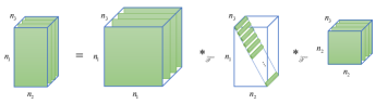
Fig. 1: An illustration of the tt-SVD factorization of a tensor with dimensions $n_{1}\times n_{2}\times n_{3}$.

Please note that

$$\hat{\mathcal{X}}^{(i)}_{\mathscr{T}}=\hat{\mathcal{U}}^{(i)}_{\mathscr{T}}\hat{\mathcal{S}}^{(i)}_{\mathscr{T}}\hat{\mathcal{V}}^{(i)H}_{\mathscr{T}},$$ (9)

and

$$\overline{\mathcal{X}_{\mathscr{T}}}=\overline{\mathcal{U}_{\mathscr{T}}}\times\overline{\mathcal{S}_{\mathscr{T}}}\times\overline{\mathcal{V}_{\mathscr{T}}}^{H},$$ (10)

i.e., in the unitary $\mathscr{T}$ transformed domain, the transformed t-SVD can be easily computed via computing the matrix SVDs of every frontal slice of $\hat{\mathcal{X}}_{\mathscr{T}}$ [4] [14] [12, 3].

subsequently, the transformed multirank [14] of $\mathcal{X}$ can be defined as a vector $\mathbf{r}\in\mathbb{R}^{n_{3}}$ with its $i$th entry being the rank of $\hat{\mathcal{X}}^{(i)}_{\mathscr{T}}$, and we then propose the transformed tensor sum rank for the first time as follows,

Definition 2 (Transformed tensor sum rank)

The transfo- rmed sum rank, termed $\operatorname{rank}_{sum}(\mathcal{X})$, is defined as the sum of the tensor multirank, i.e.,

$$\operatorname{rank}_{sum}(\mathcal{X})=\sum_{i}^{n_{3}}r_{i}=\operatorname{rank}(\overline{\mathcal{X}_{\mathscr{T}}}).$$ (11)

Based on the $\mathscr{T}$-product and the tt-SVD, we define the transformed tensor nuclear norm as follows,

Definition 3 (Transformed tensor nuclear norm)

The tran- sformed tensor nuclear norm (TTNN) of a tensor $\mathcal{X}\in\mathbb{C}^{n_{1}\times n_{2}\times n_{3}}$, denoted as $\|\mathcal{X}\|_{TTNN}$, is defined as the nuclear norm of the block diagonal matrix in the transformed domain, i.e.,

$$\|\mathcal{X}\|_{TTNN}=\|\overline{\mathcal{X}_{\mathscr{T}}}\|_{*}=\operatorname{Tr}(\overline{\mathcal{S}_{\mathscr{T}}}).$$ (12)

Please note that the TTNN is strictly derived from the dual norm of the transformed tensor spectral norm and we have proven that the TTNN is the convex envelope of the transformed tensor sum rank on a unit ball of the transformed tensor spectral norm. The derivation is detailed at Appendix.b.

3.2 The TTNN-based iterative optimization algorithm

To constrain the low rank of the dynamic MR images in the unitary transformed domain, the transformed sum rank is expected to be a small number and should be incorporated into the cost function of the reconstruction model as a constraint. While the rank constraint is not convex, we instead take the convex surrogate, the TTNN, as the minimizing constraint, and we subsequently propose a TTNN-based model and elaborately design an iterative optimization algorithm via the alternating direction method of multipliers.

The proposed TTNN-based model can be formulated as,

$$\min_{\mathcal{X}}\frac{1}{2}\|\mathscr{A}(\mathcal{X})-\mathbf{b}\|_{F}^{2}+\lambda\|\mathcal{X}\|_{TTNN},$$ (13)

where the TTNN, as the convex envelope of the transformed tensor sum rank, can enable the algorithm to exploit the tensor low-rank prior in the transformed domain to improve the reconstruction. The above optimization problem can be converted into the following constraint problem by the variable splitting strategy [28],

$$\min_{\mathcal{X}}\frac{1}{2}\|\mathscr{A}(\mathcal{X})-\mathbf{b}\|_{F}^{2}+\lambda\|\mathcal{Z}\|_{TTNN}\ \ s.t.\ \mathcal{Z}=\mathcal{X}$$ (14)

The augmented Lagrangian function of the above optimization problem is formulated by,

$$\mathscr{L}(\mathcal{X},\mathcal{Z},\mathcal{W})=\frac{1}{2}\|\mathscr{A}(\mathcal{X})-\mathbf{b}\|_{F}^{2}+\lambda\|\mathcal{Z}\|_{TTNN}+$$ (15)

$$<\mathcal{W},\mathcal{X}-\mathcal{Z}>+\frac{\mu}{2}\|\mathcal{Z}-\mathcal{X}\|_{F}^{2}$$

where $\mathcal{W}$ is the Lagrangian multiplier and $\mu>0$ is the penalty parameter. Then, carrying out a straightforward complete-the-squares procedure for the last two terms of (15), we have

$$\mathscr{L}(\mathcal{X},\mathcal{Z},\mathcal{L})=\frac{1}{2}\|\mathscr{A}(\mathcal{X})-\mathbf{b}\|_{F}^{2}+\lambda\|\mathcal{Z}\|_{TTNN}+$$ (16)

$$\frac{\mu}{2}\|\mathcal{Z}-\mathcal{X}-\mathcal{L}\|_{F}^{2}-\frac{\mu}{2}\|\mathcal{L}\|_{F}^{2}$$

where $\mathcal{L}=\frac{\mathcal{W}}{\mu}$. The problem can be efficiently solved with the alternating direction method of multipliers (ADMM) [28], resulting in the following iterative scheme:

$$\mathcal{Z}_{n}=\min_{\mathcal{Z}}\lambda\|\mathcal{Z}\|_{TTNN}+\frac{\mu}{2}\|\mathcal{Z}-\mathcal{X}_{n-1}-\mathcal{L}_{n-1}\|_{F}^{2}$$ (17)

$$\mathcal{X}_{n}=\min_{\mathcal{X}}\frac{1}{2}\|\mathscr{A}(\mathcal{X})-\mathbf{b}\|_{F}^{2}+\frac{\mu}{2}\|\mathcal{Z}_{n}-\mathcal{X}-\mathcal{L}_{n-1}\|_{F}^{2}$$ (18)

$$\mathcal{L}_{n}=\mathcal{L}_{n-1}-\eta(\mathcal{Z}_{n}-\mathcal{X}_{n})$$ (19)

where the subscript $n$ denotes the $n$th iteration and $\eta$ denotes the update rate.

3.2.1 The $\mathcal{Z}$ subproblem

The subproblem (17) can be solved by the transformed tensor singular value thresholding ($\mathscr{T}$-TSVT) operator which is detailed in Appendix.c,

$$\mathcal{Z}_{n}=\mathscr{D}_{{\lambda}/{\mu},\mathscr{T}}(\mathcal{X}_{n-1}+\mathcal{L}_{n-1}).$$ (20)

Specifically, let $\mathcal{Y}=\mathcal{X}_{n-1}+\mathcal{L}_{n-1}$ for simplification. The $\mathscr{T}$-TSVT brings $\mathcal{Y}$ into the transformed domain as $\hat{\mathcal{Y}}_{\mathscr{T}}$ by applying the unitary transform $\mathscr{T}$. Each frontal slice of the transformed data $\hat{\mathcal{Y}}_{\mathscr{T}}^{(i)}$ is then processed via the matrix singular value thresholding (SVT) [40]. Finally, the thresholding transformed tensor data is inversed by $\mathscr{T}^{H}$, i.e.,

$$\mathcal{Z}_{n}=\mathscr{T}^{H}\left[\operatorname{SVT}_{{\lambda}/{\mu}}(\mathscr{T}(\mathcal{Y}))\right]$$ (21)

3.2.2 the $\mathcal{X}$ subproblem

the subproblem (18) is a quadratic problem that can be solved analytically, i.e.,

$$\mathcal{X}_{n}=(\mathscr{A}^{H}\circ\mathscr{A}+\mu)^{-1}(\mathscr{A}^{H}(\mathbf{b})+\mu\mathcal{Z}_{n}-\mu\mathcal{L}_{n-1})$$ (22)

where the superscript $-1$ denotes the inverse of the operator and the $\circ$ represents the composition of operators or functions. If the samples are on the Cartesian grid, where $\mathscr{A}=\mathscr{S}\circ\mathscr{F}$ as shown in (1), the solution can be simplified by

$$\mathcal{X}_{n}=\mathscr{F}^{H}\left(\frac{\mathscr{S}^{H}(\mathbf{b})+\mu\mathscr{F}(\mathcal{Z}_{n}-\mathcal{L}_{n-1})}{\mathscr{S}^{H}\circ\mathscr{S}(\mathbf{1})+\mu\ \mathbf{1}}\right),$$ (23)

where $\mathbf{1}$ denotes an all-one tensor and the division operating denotes the element-wise division. Note that $\mathscr{S}^{H}:\mathbb{C}^{m}\rightarrow\mathbb{C}^{n_{1}\times n_{2}\times n_{3}}$ denotes the Hermitian transpose of the sample operator $\mathscr{S}$, and $\mathscr{S}^{H}(\mathbf{x})$ puts the element of the sampled vector $\mathbf{x}$ into the sampling location of the Cartesian grid and fills the rest with zeros.

Finally, the iterative TTNN-based algorithm obtains the following iterative procedures:

$$\begin{cases}&\mathcal{Z}_{n}=\mathscr{D}_{{\lambda}/{\mu},\mathscr{T}}(\mathcal{X}_{n-1}+\mathcal{L}_{n-1})\\ &\mathcal{X}_{n}=(\mathscr{A}^{H}\circ\mathscr{A}+\mu)^{-1}(\mathscr{A}^{H}(\mathbf{b})+\mu\mathcal{Z}_{n}-\mu\mathcal{L}_{n-1})\\ &\mathcal{L}_{n}=\mathcal{L}_{n-1}-\eta(\mathcal{Z}_{n}-\mathcal{X}_{n})\end{cases}$$ (24)

3.3 The proposed unrolling network: T²LR-Net

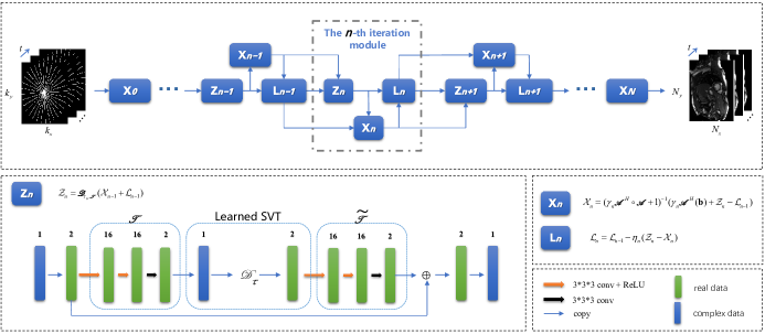
Fig. 2: The proposed T²LR-Net framework. The T²LR-Net is an unrolling neural network that unrolls N (fixed) iteration of the algorithm (25) into N iteration modules. Each iteration module contains three blocks, which we named as the transformed tensor low-rank prior block $\mathbf{Z}_{n}$, the reconstruction block $\mathbf{X}_{n}$, and the multiplier update block $\mathbf{L}_{n}$. These three blocks correspond to the three iterative steps of (25). T²LR-Net maintains the same structure as the proposed iterative TTNN-based algorithm (25), but the transformed tensor low-rank prior block is incorporated with the CNN and the hyperparameters are learned through the training process. The first row of the figure shows the T²LR-Net framework, and the second row shows the detail of the three blocks.

In traditional optimization-based methods, the reconstruction result is obtained by iteratively solving (24), where hundreds of iterations and plenty of time may be needed and the hyperparameters $\lambda,\mu,\eta$ need to be selected empirically, which is time-consuming and not robust. More importantly, the unitary transform $\mathscr{T}$ should be designed manually, which is very challenging and extremely difficult since the optimal transform $\mathscr{T}$ that makes the reconstruction precisely and rapidly convergent may be quite different for various applications.

To address the abovementioned issues, we adopt the unrolling DL strategy and unroll the TTNN-based iterative optimization algorithm into a deep neural reconstruction network, which we term T²LR-Net, to learn the transformed tensor low-rank prior adaptively from dynamic MR image datasets.

To enable our deep unrolling strategy, we generalize the optimization problem (24) into the following iterative scheme:

$$\small\begin{cases}\mathbf{Z}_{n}:&\mathcal{Z}_{n}=\mathscr{D}_{\bm{\tau}_{n},\mathscr{T}_{n}}(\mathcal{X}_{n-1}+\mathcal{L}_{n-1})\\ \mathbf{X}_{n}:&\mathcal{X}_{n}=(\gamma_{n}\mathscr{A}^{H}\circ\mathscr{A}+1)^{-1}(\gamma_{n}\mathscr{A}^{H}(\mathbf{b})+\mathcal{Z}_{n}-\mathcal{L}_{n-1})\\ \mathbf{L}_{n}:&\mathcal{L}_{n}=\mathcal{L}_{n-1}-\eta_{n}(\mathcal{Z}_{n}-\mathcal{X}_{n})\end{cases}$$ (25)

where the vector $\bm{\tau}\geq 0\in\mathbb{R}_{+}^{n_{t}}$ replaces the real number ${\lambda}/{\mu}\in\mathbb{R}_{+}$ denoting the tensor singular value threshold vector with the $i$th threshold element $\tau_{n,i}$ thresholding the $i$th frontal slice of the tensor, and $\gamma\geq 0$ replaces $1/\mu$ which is equivalent to $\mu>0$. All the hyperparameters are followed by a subscript $n$ denoting the $n$th iteration (e.g., $\bm{\tau}_{n}$), which means that the hyperparameters vary from iteration to iteration. Note that the unitary transform $\mathscr{T}_{n}$ are different in iterations to exploit various transformed tensor low-rank prior within one network or model to enhance the reconstruction performance.

Then we unroll the iterative procedures (25) into the T²LR-Net network, the framework of which is shown in Fig.2. T²LR-Net unrolls the fixed iterative steps (N) of the TTNN-based iterative optimization algorithm (25) into iteration modules, each of which contains three blocks corresponding to the three subproblems in (25), i.e., the transformed tensor low-rank prior block $\mathbf{Z}_{n}$, the reconstruction block $\mathbf{X}_{n}$, and the multiplier update block $\mathbf{L}_{n}$. The CNN is incorporated within the $\mathbf{Z}_{n}$ block to adaptively learn the best-matched transformation from the dynamic MR image datasets and the hyperparameters ($\tau,\gamma,\eta$) are also automatically learned through the training process. Next, we explain the three blocks in detail:

3.3.1 Transformed tensor low-rank prior block $\mathbf{Z}_{n}$

At this block, a learned $\mathscr{T}$-TSVT related to the $\mathcal{Z}_{n}$ subproblem in (25) is embedded into the neural network and has the same expression as (21),

$$\mathcal{Z}_{n} =\mathscr{T}_{n}^{H}\left[\operatorname{SVT}_{\bm{\tau}_{n}}(\mathscr{T}_{n}(\mathcal{X}_{n-1}+\mathcal{L}_{n-1}))\right]$$ (26)

$$\approx\widetilde{\mathscr{T}_{n}}\left[\operatorname{SVT}_{\bm{\tau}_{n}}(\mathscr{T}_{n}(\mathcal{X}_{n-1}+\mathcal{L}_{n-1}))\right].$$

Specifically, the transform $\mathscr{T}_{n}$ and the Hermitian transpose transform $\mathscr{T}_{n}^{H}$ are learned by the CNN to search for the best data-matched transformations, and the learned matrix SVT operator [27] is also incorporated to substitute the traditional SVT and adaptively determine the threshold ${\tau}_{n,t}$ of every frontal slice of the transformed image, or the threshold vector $\bm{\tau}_{n}$. For a certain frontal slice $\hat{\mathcal{Y}}_{\mathscr{T}}^{(i)}=\mathscr{T}_{n}(\mathcal{X}_{n-1}+\mathcal{L}_{n-1})=\mathbf{U}\mathbf{S}\mathbf{V}^{H}$ the learned matrix SVT utilizes the following scheme:

$$\begin{cases}\mathscr{D}_{\tau_{n,i}}(\hat{\mathcal{Y}}_{\mathscr{T}}^{(i)})&=\mathbf{U}\mathbf{S}_{\tau_{n,i}}\mathbf{V}^{H}\\ \mathbf{S}_{\tau_{n,i}}&=\operatorname{ReLU}(\mathbf{S}-\tau_{n,i})\\ \tau_{n,i}&=\operatorname{sigmoid}(a_{n,i})\cdot\max(\mathbf{S})\end{cases}$$ (27)

where we let $\mathscr{D}_{\tau_{n,i}}(\hat{\mathcal{Y}}_{\mathscr{T}}^{(i)})$ represent the SVT result of this certain frontal slice, $\operatorname{ReLU}$ denotes the rectifier linear units [41], $\operatorname{sigmoid}$ denotes the sigmoid activate function [42] and $a_{n,i}$ is set as a learnable network parameter with an initial value of -2.

Note that we do not use the Hermitian transpose transform $\mathscr{T}_{n}^{H}$ strictly, due to the complexity of strictly determining the Hermitian transpose of a CNN-learned transform. Instead, we utilize another CNN with the same structure to approximate the $\mathscr{T}_{n}^{H}$ separately, called $\widetilde{\mathscr{T}_{n}}$, and we enforce a relaxed invertibility constraint $\widetilde{\mathscr{T}_{n}}\circ\mathscr{T}_{n}=\mathbf{I}$ for handleability and practicability by incorporating it into the loss function (28) in the training process [21], of which we will further discuss the effect later in Section 5.1 and 5.2.

We divide each complex-valued data into two real-valued channels to enable the CNNs training at this block. The CNNs used in learning $\mathscr{T}_{n}$ and $\widetilde{\mathscr{T}_{n}}$ are modeled as a combination of three convolutional layers. The first two layers are 16 channels followed by a ReLU operator. The third layer is 2 channels without ReLU activation to enable the negative values of the output. The convolution kernels of all the convolutional layers are of size 3x3x3, and the stride is 1. He initialization [43] is used for the convolutional layers.

In addition, this block brings a new perspective on exploiting the low-rank prior by enforcing the low-rank constraint on a transformed domain or a feature domain induced by the CNN. Via training on the dynamic MR image dataset, CNN obtains the feature map of which the singular values are decoupled into the larger part of the distortion-free image and the smaller part of the artifact. Then, a learned threshold $\tau_{n}$ can be applied to keep as much information as the reconstruction process needs.

3.3.2 Reconstruction block $\mathbf{X}_{n}$

This block corresponds to the $\mathcal{X}_{n}$ subproblem in (25), and generate the reconstruction results. There is $\gamma_{n}=\operatorname{ReLU}(\hat{\gamma}_{n})$ where $\hat{\gamma}_{n}$ is learnable with an initial value of 0.1 in our implement.

Note that the reason why we replace $1/\mu$ in (24) with $\gamma$ in (25) is to avoid numerical instability, because $\frac{0}{0}$ would appear in the unsampled $k$-space position if the parameter $\mu$ is learned to be zero in the Cartesian sampling cases. Therefore, the introduction of $\gamma$ avoids this instability, even if $\gamma$ is learned as zero.

3.3.3 Multiplier update block $\mathbf{L}_{n}$

This block corresponds to the $\mathcal{L}_{n}$ subproblem in (25) and is used to update the Lagrange multiplier. There is $\eta_{n}=\operatorname{ReLU}(\hat{\eta}_{n})$ where $\hat{\eta}_{n}$ is learnable with an initial value of 1 in our implement.

3.4 Loss Function

The loss function of T²LR-Net is the combination of data fidelity and the invertibility constraint of the transforms, i.e.,

$$Loss=\sum_{(\bar{\mathcal{X}},\mathbf{b})\in\Omega} \|\bar{\mathcal{X}}-f_{cnn}(\mathbf{b}|\theta)\|_{F}^{2}+$$ (28)

$$\zeta\sum_{n=1}^{N} \|\widetilde{\mathscr{T}_{n}}\circ\mathscr{T}_{n}(\mathcal{X}_{n-1})-\mathcal{X}_{n-1}\|_{F}^{2},$$

where $\Omega$ denotes the given training data, $\bar{\mathcal{X}}$ is a fully sampled ground-truth data, $\mathbf{b}$ is the undersampled $k$-space data, $f_{cnn}$ denotes the output of the network, $\theta$ is the learnable parameters of the network and $\zeta$ is a hyperparameter balancing the data fidelity and the invertibility constraint of the transforms.

3.5 Parameters and Implementation Details

The learnable network parameters are the hyperparameters $\bm{\tau}_{n},\gamma_{n},\eta_{n}$ and the two CNNs corresponding to transform $\mathscr{T}_{n}$ and $\widetilde{\mathscr{T}_{n}}$ at each iteration module. The CNNs make the proposed method more adaptive and more robust to the dynamic MR image dataset. All the parameters in the iterative algorithm (25) are automatically learned by the unrolling network, which omits the tedious and unrobust process of hand-crafted parameter search.

For the hyperparameters of the network, we propose our T²LR-Net with 15 iteration modules and the hyperparameter $\zeta$ being zero, the reason for which will be discussed in Section 5.

For the T²LR-Net training, different from the scheme that uses a fixed sampling mask in the whole training process [26, 27], we take a pseudo-random mask strategy that randomly generates a certain type of sampling mask at each training step instead (e.g., radial sampling mask with 16 randomly selected lines) to enable the network to learn deeper information rather than overfitting the fixed sampling mode. During the training, the Adam optimizer [44] with parameters $\beta_{1}=0.9,\ \beta_{2}=0.999$ and $\epsilon=10^{-8}$ and the exponential decay learning rate [45] with an initial learning rate of 0.001 and a decay of 0.95 are adopted in the framework of Tensorflow [46].

4 Experiments and Results

4.1 Setup

4.1.1 Dataset

Our T²LR-Net is evaluated using the cardiac cine MRI dataset OCMR [47], which contains 57 slices of fully sampled data collected on a 3T Siemens MAGNETOM Prisma machine and 126 slices of fully sampled data on a 1.5T Siemens Avanto and a 1.5T Siemens Sola machine. To investigate the robustness of the proposed network, we use a mixed dataset under different settings, including 51 slices of the fully sampled 3T data for training, and 7 slices of 3T and 12 slices of 1.5T data for the test. We crop the training dynamic MR images into the size of $144\times 112\times 16$ ($x\times y\times t$) since the minimum data size of the training data is 288, 112, and 16, and the strides along the three dimensions are 15, 15, and 7. Thus, we obtain 1099 cardiac cine MR fully sampled images for training. For the test, 3 (out of a total of 19) slices have 2 signals averaged, and we treat each signal as a single test data, while the other 16 slices have 1 signal averaged. Thus, we obtain 22 uncropped fully sampled images for the test. Meanwhile, each of the multi-coil data in the OCMR dataset is combined into single-coil images to simplify the training process, and the coil sensitivity maps are computed by ESPIRiT [48]. For the comparison methods, we use the same training and test data for network-based methods, and only the test data are used to evaluate the performance of the optimization-based methods. Please note that the training data are cropped to the size of $144\times 112\times 16$, and the test data are uncropped, for which the testing situation is closer to the real-world situation and can also be used to evaluate the robustness of different methods.

Moreover, we also evaluate our method on the other cardiac cine MRI dataset [49], which in this paper is named TCMR for short. The TCMR dataset is comprised of short-axis cardiac cine MR images from 33 subjects. The images are scanned with a GE Genesis Signa MR scanner using the FIESTA scan protocol. A total of 399 slices with each slice of 256$\times$256$\times$20 ($x\times y\times t$) are collected. Most of the images have part of the aliasing (the pixel values of which are set to be zero) due to the undersampling with low acceleration. We only utilize distortion-free images by cutting off the aliasing. We then crop the images into the size of $128\times 128\times 16$ with the strides along the three dimensions of 15, 15, and 7. Finally, the augmented dataset with 3782 cardiac cine MR images (3392 images for training, 390 images for test) is obtained and utilized in our experiments.

4.1.2 Performance envaluation

We take signal-to-noise ratio (SNR) to be the quantitative evaluation metric,

$$\operatorname{SNR}=20\log_{10}\frac{\|Ref\|_{F}}{\|Rec-Ref\|_{F}},$$ (29)

where $Ref$ is the fully sampled ground-truth data, $Rec$ is the reconstructed image, and $\|\cdot\|_{F}$ denotes the Frobenius norm.

4.2 Retrospective Experiments

We compare the reconstruction results of the proposed T²LR-Net with four optimization-based methods (TNN, F2TNN, k-t SLR, MNN3TV) and two state-of-art unrolling network-based methods (DCCNN, SLR-Net). The TNN method exploits the low-rank prior of the FFT domain by minimizing the tensor nuclear norm [7]. The F2TNN method adopts the tt-SVD based on a compound of transforms, i.e., two-dimensional framelet transform on the spatial axis and one-dimensional FFT on the temporal axis [50], and the algorithm works via minimizing the TTNN induced by the corresponding tt-SVD. The k-t SLR method [29] utilizes the Casorati matrix low-rank prior and the total variation (TV) constraint. The MNN3TV method is the generalization of the k-t SLR method, where the Casorati matrix low-rank prior is substituted by the tensor low-rank prior via minimizing the sum of the nuclear norms of the unfolding matrices. All the optimization-based methods are conducted on an Intel Xeon W-2123 CPU, and their hyperparameters are selected empirically. For the DCCNN method, we choose a D5-C10(S) structure with 5 convolutional layers within a certain iteration, the cascade with the depth of 10, and a data sharing layer, which obtains the best performance [26]. For the SLR-Net, which utilizes the Casorati matrix low-rank prior and the transformed sparsity constraint, we choose the unrolling network with 10 iterations and set the hyperparameters consistent with the paper [27]. All the network-based methods are conducted on Tesla V100 GPU (32 GB memory) with CUDA and CUDNN support and are trained or retrained on the same dataset with 50 epochs.

We evaluate the T²LR-Net with OCMR dataset in two sampling patterns, i.e., pseudo-radial [29] with the sampling trajectory being on the Cartesian grid and variable density random sampling, and three different sampling cases are considered at each sampling pattern, where 8, 16, 30 lines are involved under radial sampling pattern and 8, 10, 12 acceleration factor (acc = the number of the sampled pixels / the total number of pixels) under the variable density random sampling pattern, as shown in Table 1, which lists the average SNRs of the different methods under these six different sampling cases on the test dataset of the OCMR. Fig.3 shows the reconstruction results of a certain test image of the OCMR dataset for the different methods under the pseudo-radial sampling pattern [29] with 16 lines, while Fig.4 shows the results on the variable density random sampling pattern with the acceleration factor of 0.125. The first row of the figures shows the reconstruction images of the different methods, and the second row shows the enlarged view of the heart regions marked by the orange box. The first image in the third row displays the sampling mask, while the other images show the reconstruction error maps w.r.t. the different methods. The fourth row and the fifth row show the x-t images indicated by the blue dot line and their reconstruction error maps. We also evaluate our proposed network on the TCMR dataset in the same six different sampling cases and shows the average reconstruction SNRs in Table 2. The visualization results of a certain image in the test dataset of TCMR are shown in Fig.5.

Table 1: The average SNRs of the different methods under two sampling patterns and six different sampling cases on the test dataset of the OCMR dataset (Mean ± Standard deviation).

methods	radial / lines			vds / acc			parameters	time / s
	8	16	30	8	10	12
TNN	12.39 ± 2.36	16.35 ± 2.68	19.66 ± 3.07	17.24 ± 2.32	15.39 ± 1.89	13.84 ± 1.74	/	20.5
F2TNN	12.43 ± 2.25	16.57 ± 2.53	19.83 ± 2.92	17.66 ± 2.35	15.45 ± 1.90	13.89 ± 1.75	/	215.6
k-t SLR	15.37 ± 2.14	18.54 ± 1.91	21.07 ± 2.31	18.83 ± 2.09	16.23 ± 1.95	14.65 ± 1.88	/	364.8
MNN3TV	17.05 ± 2.28	19.93 ± 2.32	22.10 ± 2.50	19.94 ± 2.21	16.50 ± 1.94	14.91 ± 1.83	/	3472.8
DCCNN	15.95 ± 1.79	18.53 ± 1.64	21.44 ± 2.25	20.37 ± 1.86	16.14 ± 1.80	14.48 ± 1.64	954340	1.3
SLR-Net	16.14 ± 1.87	19.24 ± 1.76	21.27 ± 2.29	20.12 ± 1.73	16.05 ± 1.64	14.40 ± 1.52	293808	3.5
T2LR-Net	19.12 ± 2.43	22.44 ± 2.60	24.08 ± 2.92	22.89 ± 2.63	16.89 ± 1.69	15.12 ± 1.66	259244	3.8

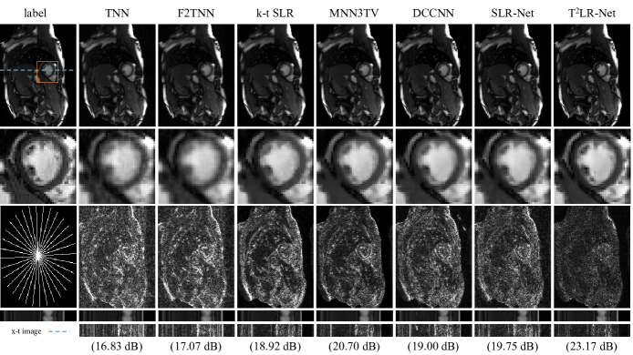
Fig. 3: The OCMR reconstruction results of different methods (TNN, F2TNN, k-t SLR, MNN3TV, DCCNN, SLR-Net and the proposed T²LR-Net) under the pseudo-radial sampling pattern [29] with 16 lines. The first row shows the reconstruction images of the different methods, and the second row shows the enlarged view of the heart regions marked by the orange box. The first image in the third row displays the sampling mask, while the other images show the reconstruction error maps w.r.t. the different methods. The fourth row and the fifth row show the x-t images indicated by the blue dot line and their reconstruction error maps. The reconstruction SNRs of different methods are listed in parentheses.

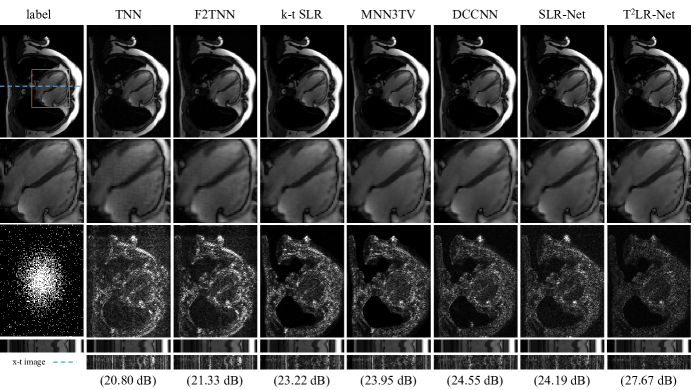
Fig. 4: The OCMR reconstruction results of the different methods (TNN, F2TNN, k-t SLR, MNN3TV, DCCNN, SLR-Net and the proposed T²LR-Net) under the variable density random sampling pattern [29] with the acceleration factor of 0.125. The first row shows the reconstruction images of the different methods, and the second row shows the enlarged view of the heart regions marked by the orange box. The first image in the third row displays the sampling mask, while the other images show the reconstruction error maps w.r.t. the different methods. The fourth row and the fifth row show the x-t images indicated by the blue dot line and their reconstruction error maps. The reconstruction SNRs of different methods are listed in parentheses.

Table 2: The average SNRs of the different methods under two sampling patterns and six different sampling cases on the test dataset of the TCMR dataset (Mean ± Standard deviation).

methods		DCCNN	SLR-Net	T2LR-Net
radial / lines	8	25.19 ± 3.08	23.71 ± 2.89	25.91 ± 3.45
	16	28.89 ± 3.39	26.72 ± 2.99	29.29 ± 3.61
	30	32.46 ± 3.43	30.36 ± 3.16	33.27 ± 3.73
variable density	8	24.63 ± 2.23	24.30 ± 2.18	24.78 ± 2.26
	10	26.85 ± 2.48	25.78 ± 2.34	27.06 ± 2.50
random / acc	12	29.36 ± 3.00	28.83 ± 2.84	29.58 ± 3.13

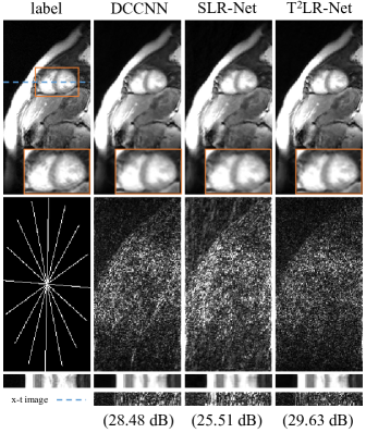
Fig. 5: The TCMR reconstruction results of the unrolling network-based methods (DCCNN, SLR-Net and the proposed T²LR-Net) under the pseudo-radial sampling pattern [29] with 8 lines. The first row shows the reconstruction images of the different methods, and the second row shows the enlarged view of the heart regions marked by the orange box. The first image in the third row displays the sampling mask, while the other images show the reconstruction error maps w.r.t. the different methods. The fourth row and the fifth row show the x-t images indicated by the blue dot line and their reconstruction error maps. The reconstruction SNRs of different methods are listed in parentheses.

The results on the two datasets indicate that our proposed T²LR-Net achieves the maximum SNR with the least parameters and obtains the minimum error and the best reconstruction performance with the sharpest edge and the clearest texture details. Note that our T²LR-Net can improve the average SNR by up to 2 dB over the second best method and up to 3 dB over the state-of-art unrolling network-based methods in some cases. The better performance of MNN3TV in contrast with that of k-t SLR indicates that the tensor low-rank prior benefits the reconstruction and has the potential to enhance the reconstruction performance. The TNN and the F2TNN methods show poor performance because the transforms that they take cannot match the MR image reconstruction problem well, although the TNN and F2TNN achieve excellent results in tensor completion tasks. The other reason for the poor appearance of TNN and F2TNN is that they only exploit the low-rank prior compared with the k-t SLR that exploits the joint intrinsic properties of low-rank prior and the TV regularization, which, from another aspect, illustrates the superiority of our proposed T²LR-Net since the T²LR-Net only takes the low-rank constraint as well while obtains more outstanding results than the methods with the combination of low rank and sparsity, such as k-t SLR, MNN3TV and SLR-Net.

4.3 Prospective Experiments

The real undersampled data that we used is from the OCMR dataset acquired on a 1.5T Siemens Avanto scanner and using the VISTA [51] sampling pattern with the 7.5 fold acceleration. We retrain the unrolling network-based methods using the same sampling mask with 50 epochs and finetune the optimization-based methods on the fully sampled OCMR training dataset as illustrated in Section 4.1.1. Note that the raw data was collected with 18 coils, while all the methods that we referred to are limited to single-coil images in this paper and the multi-coil reconstruction is not in our consideration. To tackle the multi-coil prospective reconstruction problem, we reconstruct each image of a certain coil and conduct the sum of squares on the reconstructed multi-coil images. The prospective results are shown in Fig.6. It shows that our proposed T²LR-Net makes a huge improvement over other methods, while the k-t SLR and DCCNN fail to obtain a clear image; the images from the TNN, F2TNN, MNN3TV and SLR-Net have significant artifacts. From the results, we can also indicate that our proposed T²LR-Net has a strong generalization ability from the view of the satisfying reconstruction of multi-coil images with training on a single-coil training dataset.

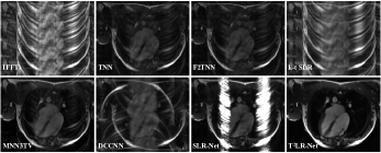
Fig. 6: The prospective results of different methods. The data is the 18-coil undersampled raw data with the VISTA sampling pattern of the OCMR dataset. The IFFT denotes the method that conducts a straightforward inverse FFT on the raw data and a sum of squares subsequently. The other methods are consistent with the Tabel 1.

5 Discussion

In this subsection, we discuss the utility of the transformed tensor low-rank prior in the network and also study the effect of internal parameters of the T²LR-Net, such as the hyperparameter of the loss function, the number of iteration modules, and the number of convolutional layers. All the networks in this section are trained in the case of a pseudo-radial sampling mask with 16 lines sampled for 50 epochs on the OCMR dataset.

5.1 The utility of the transformed tensor low-rank prior

To discuss the utility of the transformed tensor low-rank prior, we investigate two important indicators on the T²LR-Net using a certain image from the test dataset of the OCMR dataset, i.e., the number of ($\sigma<\bm{\tau}_{n}$) and the Frobenius norm $\|\widetilde{\mathscr{T}_{n}}\circ\mathscr{T}_{n}(\mathcal{X}_{n-1})-\mathcal{X}_{n-1}\|_{F}$ as shown in Fig.7. The $\sigma$ of the first one denotes the singular value of all the frontal slices of the transformed tensor $\mathscr{T}_{n}(\mathcal{X}_{n-1}+\mathcal{L}_{n-1})$ in (26) and $\bm{\tau}_{n}$ is the threshold of the SVT operator in the $n$th iteration module. This indicator, measuring the number of singular values that are less than the corresponding threshold and would be set to zero, shows the degree to which transformed tensor low-rank prior works. The second indicator is the invertibility constraint in the loss function (28) to measure the degree of the invertibility of the CNN-based transforms $\mathscr{T}_{n}$ and $\widetilde{\mathscr{T}_{n}}$ as a relaxed version of the Hermitian symmetry, and the smaller it is, the stronger the reversibility holds. Please note that the orange y-axis is backward. The figure shows that the transformed tensor low-rank prior is given more consideration at the first four iteration modules, due to the significant number of ($\sigma<\bm{\tau}_{n}$) and the relatively small Frobenius norm for the strong symmetric constraint, which is consistent with the Hermitian symmetric requirement of the transforms $\widetilde{\mathscr{T}_{n}}$ and $\mathscr{T}_{n}$ in the Equation (26). In the last eight iteration modules, the low-rank prior is no longer involved since the number of ($\sigma<\bm{\tau}_{n}$) equals 0, which indicates that the SVT operator in (26) is invalid and the transformed tensor low-rank block degenerates into a simple CNN to learn the implicit and complex prior beyond low rank to further improve the reconstruction performance, while the Frobenius norm of the transforms is increasing that the symmetric constraint is broken to release the learning ability of the CNN. Iteration modules in the middle utilize the hybrid information from both the low rank prior and the CNN-learned implicit prior.

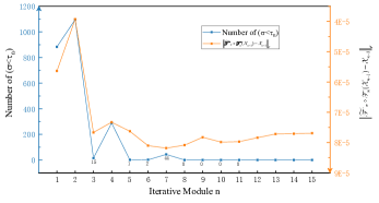
Fig. 7: The curves of the number of ($\sigma<\tau_{n}$) and the Frobenius norm $\|\widetilde{\mathscr{T}_{n}}\circ\mathscr{T}_{n}(\mathcal{X}_{n-1})-\mathcal{X}_{n-1}\|_{F}$, where the orange y-axis is backward. The $\sigma$ of the first one denotes the singular value of all the frontal slices of the transformed tensor $\mathscr{T}(\mathcal{Y})$ in (21) and $\tau_{n}$ is the threshold of the SVT operator in the $n$th iteration module. The second indicator is the invertibility constraint in the loss function (28) to measure the degree of the reversibility of the CNN-based transforms $\mathscr{T}_{n}$ and $\widetilde{\mathscr{T}_{n}}$ as a relaxed version of the Hermitian symmetry, and the smaller it is, the stronger the reversibility holds.

Fig.8 shows the reconstruction results from the iteration modules, where $\mathcal{X}_{0}$ is the input aliased image and the other $\mathcal{X}_{i}$ related to (22) is the result of the $i$th iteration module. We could find that the first four iteration modules remove the aliasing significantly with the assistance of the transformed tensor low-rank prior from the information that Fig.7 gives and the reconstruction performance of $\mathcal{X}_{4}$ w.r.t. $\mathcal{X}_{0}$; the middle modules further preserve the edges and the texture details comparing $\mathcal{X}_{7}$ with $\mathcal{X}_{4}$; the last eight modules adaptively suppress the noise and smooth the tissues via the flexible learning CNN from the difference between $\mathcal{X}_{15}$ and $\mathcal{X}_{7}$.

To sum up, our proposed T²LR-Net not only utilizes the transformed tensor low-rank prior but also incorporates the CNN-learned flexible and implicit prior by setting the number of ($\sigma<\bm{\tau}_{n}$) to zero to omit the SVT operation and enable the strong learning ability of CNN, and the balance between the low-rank and the CNN-based prior is adjusted adaptively via the training process and from the dataset.

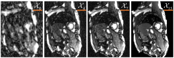
Fig. 8: The reconstruction results from the iteration modules, where $\mathcal{X}_{0}$ is the input aliased image and the other $\mathcal{X}_{i}$ related to (22) is the result of the $i$th iteration module.

5.2 Effect of hyperparameter of the loss function

We investigate the effect of the hyperparameter $\zeta$ of the loss function by retraining different networks with different $\zeta$. The reconstruction SNRs on the test dataset of the OCMR are shown in Fig.9. The average SNR of the test data increases from 17.17 dB to 22.27 dB with decreasing hyperparameter $\zeta$ from 1e-1 to 1e-4. It is foreseeable that $\zeta=0$ may be the best choice for the T²LR-Net, and it obtains 22.44 dB (the best) average SNR, as the figure shows.

Although the relaxed left invertibility constraint instead of Hermitian symmetry is adopted, it is shown that the relaxed one still limits the learning ability of the CNNs and results in worse performance with increasing the weight of the invertibility constraint in the loss function. According to Section 5.1, the constraint prevents the embedded CNNs from learning the beneficially implicit prior, since $\mathscr{T}_{n}\circ\widetilde{\mathscr{T}_{n}}(\mathcal{X})=\mathcal{X}$ if the invertibility constraint holds. In that case, the CNNs in the iteration modules where the number of ($\sigma<\tau_{n}$) equals 0 are useless but increase memory cost and computational complexity. Therefore, the stronger the invertibility constraint is, the poorer the reconstruction results are. From the analysis and the reconstruction performance, we propose our T²LR-Net with $\zeta=0$ of the loss function, i.e., using the mean squared error loss function only.

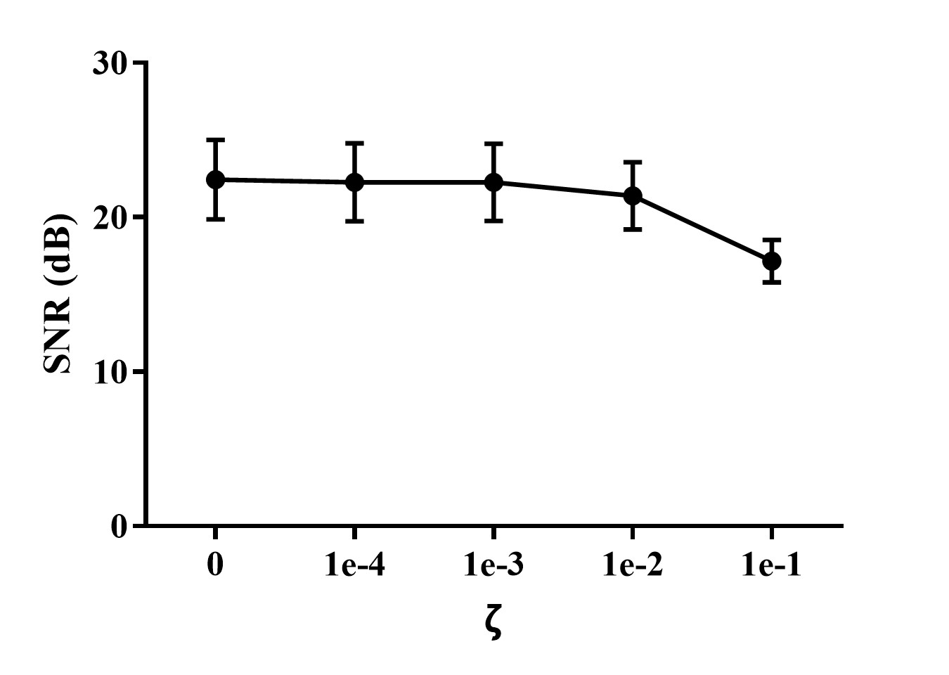
Fig. 9: Effect of hyperparameter $\zeta$ of the loss function. The x-axis except 0 is shown on the logarithmic scale. The figure shows the change in SNR values on the test data of OCMR as varying the hyperparameter $\zeta$ from 1e-1 to 1e-4. The dot represents the mean SNR, and the bar represents the standard deviation of SNR. The mean SNR of the test data increases from 17.17 dB to 22.27 dB with decreasing hyperparameter $\zeta$ from 1e-1 to 1e-4. It is foreseeable that $\zeta=0$ may be the best choice for the T²LR-Net, and it obtains 22.44 dB (the best) mean SNR.

5.3 Effect of the number of iteration modules

In this case, we retrain the networks with 5, 10, 15 and 20 iteration modules and compare the reconstruction results on the test dataset of OCMR to investigate the effect of the number of iteration modules, as the results are shown in Table 3. From the results, The difference between 15 and 20 iteration modules is not as obvious as that between 10 and 15 iteration modules, i.e., 15 iteration modules may be enough to learn most of the information needed for dynamic MR image reconstruction. Thus, we propose our T²LR-Net with 15 iteration modules, but please note that the performance should be better if one uses more iteration modules than 15 without the efficiency consideration.

Table 3: Effect of the number of iteration modules. The SNR values are shown in the form of Mean ± Standard deviation.

num	5	10	15	20
SNR(dB)	19.38 ± 1.78	21.70 ± 2.38	22.44 ± 2.58	22.71 ± 2.66

Table 4: Effect of the number of the convolutional layers. The conv num denotes the number of the 16-channels convolutional layers. The SNR values are shown in the form of Mean ± standard deviation.

conv num	1	2	3	4
SNR (dB)	21.30 ± 2.38	22.44 ± 2.58	22.56 ± 2.60	22.02 ± 2.39

5.4 Effect of the number of the convolutional layers

We restate that each iteration module contains two CNNs, each of which contains two convolutional layers with 16 channels and one convolutional layer with 2 channels. The 2-channels layer is special for enabling the real-valued data in convolutional layers to stack back into complex values. Thus, we investigate the effect of the number of the 16-channels convolutional layers in the CNNs, e.g., the T²LR-Net that we proposed has 2 convolutional layers with 16 channels. The results are shown in Table 4. The networks that contain different 16-channels convolutional layers are retrained on the OCMR datasets with 15 iteration modules and $\zeta=0$. It shows that one 16-channel layer is too simple to learn the transforms well, and four 16-channel convolutional layers make the network too deep that may overfit the training data resulting in a worse performance. Two 16-channel convolutional layers are the best choice for T²LR-Net since it obtains satisfying results and saves training costs.

5.5 Limitations and prosepcts

The SVT operator in each iteration module needs to calculate the singular value decomposition, which is nondifferentiable in some conditions, such as the matrix to be solved containing repeated singular values, probably leading to the abortion of the training for the NaN gradients. In addition, the hybrid utility of transformed low-rank and CNN-learned prior confuses the deep understanding of the mathematical properties of the transform that induces the transformed tensor nuclear norm. We will exploit the differentiable surrogates of the SVD and design the separation experiments to analyze the inherence of the transforms in future works.

6 Conclusion

We propose an unrolling reconstruction network learning transformed tensor low-rank prior for dynamic MR imaging. By generalizing the traditional t-SVD into the transformed version with arbitrary unitary transform, we enable the proposed TTNN-based model to exploit the tensor low-rank prior in the transformed domain and elaborately design an iterative optimization algorithm based on ADMM to optimize the reconstruction result. Furthermore, the TTNN-based iterative algorithm is unrolled into a deep neural network, while the CNN is incorporated to learn the best-matched transformation from the dynamic MR dataset and the parameters of the original iterative algorithm are also learned through the training progress. Our proposed T²LR-Net also provides a new prospect of utilizing the low-rank prior in the CNN extracted feature domain. Retrospective and prospective experiments demonstrated a significant improvement over the state-of-art optimization-based and unrolling network-based methods.

Appendix

a. Additional definations

The identity tensor is defined based on the $\mathscr{T}$-product, and makes the following equality satisfied given $\mathcal{A}\in\mathbb{C}^{n_{1}\times n_{2}\times n_{3}}$,

$$(\mathcal{I}_{\mathscr{T}})_{n_{1}}*_{\mathscr{T}}\mathcal{A}=\mathcal{A}*_{\mathscr{T}}(\mathcal{I}_{\mathscr{T}})_{n_{2}}=\mathcal{A},$$ (30)

where $(\mathcal{I}_{\mathscr{T}})_{n_{1}}\in\mathbb{C}^{n_{1}\times n_{1}\times n_{3}}$ is the identity tensor with the first two dimensions equal to $n_{1}$.

In the similar way, the Hermitian transpose of a tensor $\mathcal{A}\in\mathbb{C}^{n_{1}\times n_{2}\times n_{3}}$ is the tensor $\mathcal{A}^{H}\in\mathbb{C}^{n_{2}\times n_{1}\times n_{3}}$, defined as

$$\mathcal{A}^{H}=\mathscr{T}^{H}[\operatorname{fold}(\overline{\mathcal{A}_{\mathscr{T}}}^{H})],$$ (31)

and the unitary tensor $\mathcal{Q}\in\mathbb{C}^{n\times n\times n_{3}}$ is defined as

$$\mathcal{Q}^{H}*_{\mathscr{T}}\mathcal{Q}=\mathcal{Q}*_{\mathscr{T}}\mathcal{Q}^{H}=\mathcal{I}_{\mathscr{T}}$$ (32)

The definitions and the properties of Frobenius norm and inner product [4] are denoted as follows,

$$\|\mathcal{A}\|_{F}=\sqrt{\sum_{ijk}|a_{ijk}|^{2}}=\|\hat{\mathcal{A}}_{\mathscr{T}}\|_{F}=\|\overline{\mathcal{A}_{\mathscr{T}}}\|_{F},$$ (33)

$$<\mathcal{A},\mathcal{B}>=\sum_{i=1}^{n_{3}}<\mathcal{A}^{(i)},\mathcal{B}^{(i)}>=<\mathcal{A}_{\mathscr{T}},\mathcal{B}_{\mathscr{T}}>$$ (34)

$$=<\overline{\mathcal{A}_{\mathscr{T}}},\overline{\mathcal{B}_{\mathscr{T}}}>,$$

where $\mathcal{A}\in\mathbb{C}^{n_{1}\times n_{2}\times n_{3}}$, $\mathcal{B}\in\mathbb{C}^{n_{2}\times n_{4}\times n_{3}}$ and the above equalities are satisfied due to the fact that the unitary transform $\mathscr{T}$ preserves the Frobenius norm and inner product [39].

b. The derivation of the transformed tensor nuclear norm

Followed from the derivation in [4], the transformed tensor spectral norm w.r.t. $\mathscr{T}$, termed $\|\mathcal{X}\|_{\mathscr{T}}$, induced by the Frobenius-normed operator norm, is defined by the matrix spectral norm of $\overline{\mathcal{X}_{\mathscr{T}}}$, i.e.,

$$\|\mathcal{X}\|_{\mathscr{T}}=\|\overline{\mathcal{X}_{\mathscr{T}}}\|.$$ (35)

Then, according to the truth that the nuclear norm is the dual norm of the spectral norm, we define the transformed tensor nuclear norm, termed $\|\mathcal{X}\|_{TTNN}$, as the dual norm of the transformed tensor spectral norm [4]. For any $\mathcal{A}\in\mathbb{C}^{n_{1}\times n_{2}\times n_{3}}$, by (34) and (35), we have

$$\|\mathcal{X}\|_{TTNN} =\mathop{\operatorname{sup}}_{\|\mathcal{A}\|_{\mathscr{T}}\leq 1}<\mathcal{X},\mathcal{A}>$$ (36)

$$=\mathop{\operatorname{sup}}_{\|\overline{\mathcal{A}_{\mathscr{T}}}\|\leq 1}<\overline{\mathcal{X}_{\mathscr{T}}},\overline{\mathcal{A}_{\mathscr{T}}}>$$ (37)

$$\leq\mathop{\operatorname{sup}}_{\|\widetilde{\mathcal{A}}\|\leq 1}<\overline{\mathcal{X}_{\mathscr{T}}},\widetilde{\mathcal{A}}>$$ (38)

$$=\|\overline{\mathcal{X}_{\mathscr{T}}}\|_{*},$$ (39)

where $\overline{\mathcal{X}_{\mathscr{T}}}=\operatorname{bdiag}(\hat{\mathcal{X}}_{\mathscr{T}})$ as it is in (4), equation (37) is from (34) and (35), equation (38) is because we relax the block diagonal matrix $\overline{\mathcal{A}_{\mathscr{T}}}$ into an arbitrary matrix $\widetilde{\mathcal{A}}\in\mathbb{C}^{n_{1}\times n_{1}\times n_{3}}$, equation (39) holds due to that the matrix nuclear norm is the dual norm of the matrix spectral norm. Then, we show the equality (38) holds and thus $\|\mathcal{X}\|_{TTNN}=\|\overline{\mathcal{X}_{\mathscr{T}}}\|_{*}$. If $\mathcal{X}=\mathcal{U}*_{\mathscr{T}}\mathcal{S}*_{\mathscr{T}}\mathcal{V}^{H}$, we find an $\mathcal{A}=\mathcal{U}*_{\mathscr{T}}\mathcal{V}^{H}$, then we have,

$$<\mathcal{X},\mathcal{A}> =<\mathcal{U}*_{\mathscr{T}}\mathcal{S}*_{\mathscr{T}}\mathcal{V}^{H},\mathcal{U}*_{\mathscr{T}}\mathcal{V}^{H}>=$$ (40)

$$<\overline{\mathcal{X}_{\mathscr{T}}},\overline{\mathcal{A}_{\mathscr{T}}}> =<\overline{\mathcal{U}*_{\mathscr{T}}\mathcal{S}*_{\mathscr{T}}\mathcal{V}^{H}},\overline{\mathcal{U}*_{\mathscr{T}}\mathcal{V}^{H}}>$$ (41)

$$=<\overline{\mathcal{U}_{\mathscr{T}}}\times\overline{\mathcal{S}_{\mathscr{T}}}\times\overline{\mathcal{V}_{\mathscr{T}}}^{H},\overline{\mathcal{U}_{\mathscr{T}}}\times\overline{\mathcal{V}_{\mathscr{T}}}^{H}>$$ (42)

$$=\operatorname{Tr}(\overline{\mathcal{S}_{\mathscr{T}}})$$ (43)

$$=\|\overline{\mathcal{X}_{\mathscr{T}}}\|_{*},$$ (44)

where equation (42) is from (7), and equation (43) is from the unitary property of $\mathcal{U}$ and $\mathcal{V}$, (44) holds due to the fact that the matrix nuclear norm is calculated by the sum of singular values.Thus, we have the definition of the transformed tensor nuclear norm (Definition.3).

Please note that the matrix nuclear norm $\|\overline{\mathcal{X}_{\mathscr{T}}}\|_{*}$ is the convex envelope of the matrix rank $\operatorname{rank}(\overline{\mathcal{X}_{\mathscr{T}}})$ within the set $\{\overline{\mathcal{X}_{\mathscr{T}}}|\|\overline{\mathcal{X}_{\mathscr{T}}}\|\leq 1\}$. Thus, from (11), (12) and (35), the transformed tensor nuclear norm $\|\mathcal{X}\|_{TTNN}$ is the convex envelope of the transformed tensor sum rank $\operatorname{rank}_{sum}(\mathcal{X})$ on a unit ball of transformed tensor spectral norm $\{\mathcal{X}\in\mathbb{C}^{n_{1}\times n_{2}\times n_{3}}|\|\mathcal{X}\|_{\mathscr{T}}\leq 1\}$.

c. The derivation of transformed tensor singular value thresholding

Based on the definition of TTNN, the transformed tensor singular value thresholding ($\mathscr{T}$-TSVT) [4] [14] is shown as follows.

For any $\tau>0$ and $\mathcal{Y}=\mathcal{U}*_{\mathscr{T}}\mathcal{S}*_{\mathscr{T}}\mathcal{V}^{H}\in\mathbb{C}^{n_{1}\times n_{2}\times n_{3}}$, the closed solution of the following optimization problem is given by,

$$\mathscr{D}_{\tau,\mathscr{T}}(\mathcal{Y})=\arg\min_{\mathcal{X}}\tau\|\mathcal{X}\|_{TTNN}+\frac{1}{2}\|\mathcal{X}-\mathcal{Y}\|_{F}^{2},$$ (45)

where $\mathscr{D}_{\tau,\mathscr{T}}$ denotes the $\mathscr{T}$-TSVT operator, and

$$\mathscr{D}_{\tau,\mathscr{T}}(\mathcal{Y}) =\mathcal{U}*_{\mathscr{T}}\mathcal{S}_{\tau}*_{\mathscr{T}}\mathcal{V}^{H}$$ (46)

$$=\mathscr{T}^{H}\left(\operatorname{fold}\left(\overline{\mathcal{U}_{\mathscr{T}}}\times\overline{\mathcal{S}_{\mathscr{T}},\tau}\times\overline{\mathcal{V}_{\mathscr{T}}}^{H}\right)\right),$$

where $\mathcal{S}_{\tau}=\mathscr{T}^{H}(\operatorname{fold}(\overline{\mathcal{S}_{\mathscr{T},,\tau}}))$ and $\overline{\mathcal{S}_{\mathscr{T}},\tau}=\max(\overline{\mathcal{S}_{\mathscr{T}}}-\tau,0)$.

From (12) and (33), the result of the $\mathscr{T}$-TSVT operator can be obtained from the following matrix optimization problem,

$$\mathscr{D}_{\tau,\mathscr{T}}(\mathcal{Y})=$$ (47)

$$\mathscr{T}^{H}\left(\operatorname{fold}\left(\mathop{\arg\min}_{\overline{\mathcal{X}_{\mathscr{T}}}}\tau\|\overline{\mathcal{X}_{\mathscr{T}}}\|_{*}+\frac{1}{2}\|\overline{\mathcal{X}_{\mathscr{T}}}-\overline{\mathcal{Y}_{\mathscr{T}}}\|_{F}^{2}\right)\right),$$

where $\overline{\mathcal{Y}_{\mathscr{T}}}=\overline{\mathcal{U}_{\mathscr{T}}}\times\overline{\mathcal{S}_{\mathscr{T}}}\times\overline{\mathcal{V}_{\mathscr{T}}}^{H}$, and the closed solution of the inside matrix optimization problem is given by the matrix SVT operator $\mathscr{D}_{\tau}$ [40],

$$\mathscr{D}_{\tau}(\overline{\mathcal{Y}_{\mathscr{T}}})=\overline{\mathcal{U}_{\mathscr{T}}}\times\overline{\mathcal{S}_{\mathscr{T}},\tau}\times\overline{\mathcal{V}_{\mathscr{T}}}^{H}.$$ (48)

Thus, the equation (46) holds.

Namely, the $\mathscr{T}$-TSVT operator first transforms $\mathcal{Y}$ into the unitary $\mathscr{T}$ transformed domain to obtain $\hat{\mathcal{Y}}_{\mathscr{T}}$. Then the matrix SVT is applied on every frontal slice of $\hat{\mathcal{Y}}_{\mathscr{T}}=\hat{\mathcal{U}}_{\mathscr{T}}\hat{\mathcal{S}}_{\mathscr{T}}\hat{\mathcal{V}}^{H}_{\mathscr{T}}$, i.e., for the $i$th frontal slice, $\mathscr{D}_{\tau}(\hat{\mathcal{Y}}^{(i)}_{\mathscr{T}})=\hat{\mathcal{U}}^{(i)}_{\mathscr{T}}\hat{\mathcal{S}}^{(i)}_{\mathscr{T},\tau}\hat{\mathcal{V}}^{(i)H}_{\mathscr{T}}$. Finally, $\mathscr{T}^{H}$ is applied to convert the image back to the original image domain.

References

- [1] T. G. Kolda and B. W. Bader, “Tensor decompositions and applications,” SIAM review, vol. 51, no. 3, pp. 455–500, 2009.
- [2] B. Romera-Paredes and M. Pontil, “A new convex relaxation for tensor completion,” Advances in neural information processing systems, vol. 26, 2013.
- [3] M. E. Kilmer and C. D. Martin, “Factorization strategies for third-order tensors,” Linear Algebra and its Applications, vol. 435, no. 3, pp. 641–658, 2011.
- [4] C. Lu, J. Feng, Y. Chen, W. Liu, Z. Lin, and S. Yan, “Tensor robust principal component analysis with a new tensor nuclear norm,” IEEE transactions on pattern analysis and machine intelligence, vol. 42, no. 4, pp. 925–938, 2019.
- [5] H. Zeng, X. Xie, H. Cui, H. Yin, and J. Ning, “Hyperspectral image restoration via global l 1-2 spatial–spectral total variation regularized local low-rank tensor recovery,” IEEE Transactions on Geoscience and Remote Sensing, vol. 59, no. 4, pp. 3309–3325, 2020.
- [6] Y. Chen, S. Wang, C. Peng, Z. Hua, and Y. Zhou, “Generalized nonconvex low-rank tensor approximation for multi-view subspace clustering,” IEEE Transactions on Image Processing, vol. 30, pp. 4022–4035, 2021.
- [7] Z. Zhang and S. Aeron, “Exact tensor completion using t-svd,” IEEE Transactions on Signal Processing, vol. 65, no. 6, pp. 1511–1526, 2016.
- [8] C. Lu, J. Feng, Y. Chen, W. Liu, Z. Lin, and S. Yan, “Tensor robust principal component analysis: Exact recovery of corrupted low-rank tensors via convex optimization,” in Proceedings of the IEEE conference on computer vision and pattern recognition, 2016, pp. 5249–5257.
- [9] Y. Zhang and Y. Hu, “Dynamic cardiac mri reconstruction using combined tensor nuclear norm and casorati matrix nuclear norm regularizations,” in 2022 IEEE 19th International Symposium on Biomedical Imaging (ISBI). IEEE, 2022, pp. 1–4.
- [10] J.-L. Wang, T.-Z. Huang, X.-L. Zhao, T.-X. Jiang, and M. K. Ng, “Multi-dimensional visual data completion via low-rank tensor representation under coupled transform,” IEEE Transactions on Image Processing, vol. 30, pp. 3581–3596, 2021.
- [11] T.-X. Jiang, M. K. Ng, X.-L. Zhao, and T.-Z. Huang, “Framelet representation of tensor nuclear norm for third-order tensor completion,” IEEE Transactions on Image Processing, vol. 29, pp. 7233–7244, 2020.
- [12] E. Kernfeld, M. Kilmer, and S. Aeron, “Tensor–tensor products with invertible linear transforms,” Linear Algebra and its Applications, vol. 485, pp. 545–570, 2015.
- [13] C. Lu, X. Peng, and Y. Wei, “Low-rank tensor completion with a new tensor nuclear norm induced by invertible linear transforms,” in Proceedings of the IEEE/CVF Conference on Computer Vision and Pattern Recognition, 2019, pp. 5996–6004.
- [14] G. Song, M. K. Ng, and X. Zhang, “Robust tensor completion using transformed tensor singular value decomposition,” Numerical Linear Algebra with Applications, vol. 27, no. 3, p. e2299, 2020.
- [15] M. K. Ng, X. Zhang, and X.-L. Zhao, “Patched-tube unitary transform for robust tensor completion,” Pattern Recognition, vol. 100, p. 107181, 2020.
- [16] D. Qiu, M. Bai, M. K. Ng, and X. Zhang, “Robust low-rank tensor completion via transformed tensor nuclear norm with total variation regularization,” Neurocomputing, vol. 435, pp. 197–215, 2021.
- [17] P.-P. Wang, L. Li, and G.-H. Cheng, “Low-rank tensor completion with sparse regularization in a transformed domain,” Numerical Linear Algebra with Applications, vol. 28, no. 6, p. e2387, 2021.
- [18] Y. LeCun, Y. Bengio, and G. Hinton, “Deep learning,” nature, vol. 521, no. 7553, pp. 436–444, 2015.
- [19] K. Gregor and Y. LeCun, “Learning fast approximations of sparse coding,” in Proceedings of the 27th international conference on international conference on machine learning, 2010, pp. 399–406.
- [20] N. Shlezinger, Y. C. Eldar, and S. P. Boyd, “Model-based deep learning: On the intersection of deep learning and optimization,” arXiv preprint arXiv:2205.02640, 2022.
- [21] J. Zhang and B. Ghanem, “Ista-net: Interpretable optimization-inspired deep network for image compressive sensing,” in Proceedings of the IEEE conference on computer vision and pattern recognition, 2018, pp. 1828–1837.
- [22] J. Sun, H. Li, Z. Xu et al., “Deep admm-net for compressive sensing mri,” Advances in neural information processing systems, vol. 29, 2016.
- [23] H. K. Aggarwal, M. P. Mani, and M. Jacob, “Modl: Model-based deep learning architecture for inverse problems,” IEEE transactions on medical imaging, vol. 38, no. 2, pp. 394–405, 2018.
- [24] C. Qin, J. Schlemper, J. Caballero, A. N. Price, J. V. Hajnal, and D. Rueckert, “Convolutional recurrent neural networks for dynamic mr image reconstruction,” IEEE transactions on medical imaging, vol. 38, no. 1, pp. 280–290, 2018.
- [25] J. Xiang, Y. Dong, and Y. Yang, “Fista-net: Learning a fast iterative shrinkage thresholding network for inverse problems in imaging,” IEEE Transactions on Medical Imaging, vol. 40, no. 5, pp. 1329–1339, 2021.
- [26] J. Schlemper, J. Caballero, J. V. Hajnal, A. N. Price, and D. Rueckert, “A deep cascade of convolutional neural networks for dynamic mr image reconstruction,” IEEE transactions on Medical Imaging, vol. 37, no. 2, pp. 491–503, 2017.
- [27] Z. Ke, W. Huang, Z.-X. Cui, J. Cheng, S. Jia, H. Wang, X. Liu, H. Zheng, L. Ying, Y. Zhu et al., “Learned low-rank priors in dynamic mr imaging,” IEEE Transactions on Medical Imaging, vol. 40, no. 12, pp. 3698–3710, 2021.
- [28] M. V. Afonso, J. M. Bioucas-Dias, and M. A. Figueiredo, “Fast image recovery using variable splitting and constrained optimization,” IEEE transactions on image processing, vol. 19, no. 9, pp. 2345–2356, 2010.
- [29] S. G. Lingala, Y. Hu, E. DiBella, and M. Jacob, “Accelerated dynamic mri exploiting sparsity and low-rank structure: kt slr,” IEEE transactions on medical imaging, vol. 30, no. 5, pp. 1042–1054, 2011.
- [30] B. Trémoulhéac, N. Dikaios, D. Atkinson, and S. R. Arridge, “Dynamic mr image reconstruction–separation from undersampled (k, t)-space via low-rank plus sparse prior,” IEEE transactions on medical imaging, vol. 33, no. 8, pp. 1689–1701, 2014.
- [31] F. Shi, J. Cheng, L. Wang, P.-T. Yap, and D. Shen, “Lrtv: Mr image super-resolution with low-rank and total variation regularizations,” IEEE transactions on medical imaging, vol. 34, no. 12, pp. 2459–2466, 2015.
- [32] K. Cui, “Dynamic mri reconstruction via weighted tensor nuclear norm regularizer,” IEEE Journal of Biomedical and Health Informatics, vol. 25, no. 8, pp. 3052–3060, 2021.
- [33] S. F. Roohi, D. Zonoobi, A. A. Kassim, and J. L. Jaremko, “Multi-dimensional low rank plus sparse decomposition for reconstruction of under-sampled dynamic mri,” Pattern Recognition, vol. 63, pp. 667–679, 2017.
- [34] X. Yang, Y. Luo, S. Chen, X. Zhen, Q. Yu, and K. Liu, “Dynamic mri reconstruction from highly undersampled (k, t)-space data using weighted schatten p-norm regularizer of tensor,” Magnetic resonance imaging, vol. 37, pp. 260–272, 2017.
- [35] Y. Liu, T. Liu, J. Liu, and C. Zhu, “Smooth robust tensor principal component analysis for compressed sensing of dynamic mri,” Pattern Recognition, vol. 102, p. 107252, 2020.
- [36] J. Ai, S. Ma, H. Du, and L. Fang, “Dynamic mri reconstruction using tensor-svd,” in 2018 14th IEEE International Conference on Signal Processing (ICSP). IEEE, 2018, pp. 1114–1118.
- [37] S. Ma, H. Du, Q. Wu, and W. Mei, “Dynamic mri reconstruction exploiting partial separability and t-svd,” in 2019 IEEE 7th International Conference on Bioinformatics and Computational Biology (ICBCB). IEEE, 2019, pp. 179–184.
- [38] S. Biswas, H. K. Aggarwal, and M. Jacob, “Dynamic mri using model-based deep learning and storm priors: Modl-storm,” Magnetic resonance in medicine, vol. 82, no. 1, pp. 485–494, 2019.
- [39] R. A. Horn and C. R. Johnson, Matrix analysis. Cambridge university press, 2012.
- [40] J.-F. Cai, E. J. Candès, and Z. Shen, “A singular value thresholding algorithm for matrix completion,” SIAM Journal on optimization, vol. 20, no. 4, pp. 1956–1982, 2010.
- [41] X. Glorot, A. Bordes, and Y. Bengio, “Deep sparse rectifier neural networks,” in Proceedings of the fourteenth international conference on artificial intelligence and statistics. JMLR Workshop and Conference Proceedings, 2011, pp. 315–323.
- [42] I. Goodfellow, Y. Bengio, and A. Courville, Deep learning. MIT press, 2016.
- [43] K. He, X. Zhang, S. Ren, and J. Sun, “Delving deep into rectifiers: Surpassing human-level performance on imagenet classification,” in Proceedings of the IEEE international conference on computer vision, 2015, pp. 1026–1034.
- [44] D. P. Kingma and J. Ba, “Adam: A method for stochastic optimization,” arXiv preprint arXiv:1412.6980, 2014.
- [45] M. D. Zeiler, “Adadelta: an adaptive learning rate method,” arXiv preprint arXiv:1212.5701, 2012.
- [46] M. Abadi, P. Barham, J. Chen, Z. Chen, A. Davis, J. Dean, M. Devin, S. Ghemawat, G. Irving, M. Isard et al., “TensorFlow: A system for Large-Scale machine learning,” in 12th USENIX symposium on operating systems design and implementation (OSDI 16), 2016, pp. 265–283.
- [47] C. Chen, Y. Liu, P. Schniter, M. Tong, K. Zareba, O. Simonetti, L. Potter, and R. Ahmad, “Ocmr (v1. 0)–open-access multi-coil k-space dataset for cardiovascular magnetic resonance imaging,” arXiv preprint arXiv:2008.03410, 2020.
- [48] M. Uecker, P. Lai, M. J. Murphy, P. Virtue, M. Elad, J. M. Pauly, S. S. Vasanawala, and M. Lustig, “Espirit—an eigenvalue approach to autocalibrating parallel mri: where sense meets grappa,” Magnetic resonance in medicine, vol. 71, no. 3, pp. 990–1001, 2014.
- [49] A. Andreopoulos and J. K. Tsotsos, “Efficient and generalizable statistical models of shape and appearance for analysis of cardiac mri,” Medical image analysis, vol. 12, no. 3, pp. 335–357, 2008.
- [50] J.-L. Wang, T.-Z. Huang, X.-L. Zhao, T.-X. Jiang, and M. K. Ng, “Multi-dimensional visual data completion via low-rank tensor representation under coupled transform,” IEEE Transactions on Image Processing, vol. 30, pp. 3581–3596, 2021.
- [51] R. Ahmad, H. Xue, S. Giri, Y. Ding, J. Craft, and O. P. Simonetti, “Variable density incoherent spatiotemporal acquisition (vista) for highly accelerated cardiac mri,” Magnetic resonance in medicine, vol. 74, no. 5, pp. 1266–1278, 2015.