Final m/s version of paper accepted for publication in Neural Computation. Inference and Learning for Generative Capsule Models

Abstract

Capsule networks (see e.g. Hinton et al.,, 2018) aim to encode knowledge of and reason about the relationship between an object and its parts. In this paper we specify a generative model for such data, and derive a variational algorithm for inferring the transformation of each model object in a scene, and the assignments of observed parts to the objects. We derive a learning algorithm for the object models, based on variational expectation maximization (Jordan et al.,, 1999). We also study an alternative inference algorithm based on the RANSAC method of Fischler and Bolles, (1981). We apply these inference methods to (i) data generated from multiple geometric objects like squares and triangles (“constellations”), and (ii) data from a parts-based model of faces. Recent work by Kosiorek et al., (2019) has used amortized inference via stacked capsule autoencoders (SCAEs) to tackle this problem—our results show that we significantly outperform them where we can make comparisons (on the constellations data).

Keywords: Capsules, variational inference, permutation matrix, Sinkhorn-Knopp algorithm, RANSAC.

1 Introduction

An attractive way to set up the problem of object recognition is hierarchically, where an object is described in terms of its parts, and these parts are in turn composed of sub-parts, and so on. For example a face can be described in terms of the eyes, nose, mouth, hair, etc.; and a teapot can be described in terms of a body, handle, spout and lid parts. This approach has a long history in computer vision, see e.g. the work on Pictoral Structures by Fischler and Elschlager, (1973), and Recognition-by-Components by Biederman, (1987). More recently Felzenszwalb et al., (2009) used discriminatively-trained parts-based models to obtain state-of-the-art results (at the time) for object recognition. Advantages of recognizing objects by first recognizing their constituent parts include tolerance to the occlusion of some parts, and that parts may vary less under a change of pose than the appearance of the whole object.

Recent work by Sabour et al., (2017) and Hinton et al., (2018) has developed capsule networks. These exploit the fact that if the pose of the object changes, this can have very complicated effects on the pixel intensities in an image, but the geometric transformation between the object and the parts can be described by a simple linear transformation (as used in computer graphics). In these papers a part in a lower level can vote for the pose of an object in the higher level, and an object’s presence is established by the agreement between votes for its pose in a process called “routing-by-agreement”. Hinton et al., (2018, p. 1) describe this as a process which “updates the probability with which a part is assigned to a whole based on the proximity of the vote coming from that part to the votes coming from other parts that are assigned to that whole”. Subsequently Kosiorek et al., (2019) framed inference for a capsule network in terms of an autoencoder, the Stacked Capsule Autoencoder (SCAE). Here, instead of the iterative routing-by-agreement algorithm, a neural network $h^{\mathrm{caps}}$ takes as input the set of input parts and outputs predictions for the object capsules’ instantiation parameters $\{{\mathbf{y}}_{k}\}_{k=1}^{K}$. Further networks $h_{k}^{\mathrm{part}}$ are then used to predict part candidates from each ${\mathbf{y}}_{k}$.

The objective function used in Hinton et al., (2018) (their eq. 4) is quite complex (involving four separate terms), and is not derived from first principles. In this paper we argue that the description in the paragraph above is backwards—we find it more natural to first describe the generative process by which an object gives rise to its parts, and that the appropriate routing-by-agreement inference algorithm then falls out naturally from this principled formulation.

The contributions of this paper are to:

• Derive a novel variational inference algorithm for routing-by-agreement, based on a generative model of object-part relationships, including a relaxation of the permutation-matrix formulation for matching object parts to observations;

• Focus on the problem of inference for scenes containing multiple objects. Much of the work on capsules considers only single objects (although sec. 6 in Sabour et al., (2017) and De Sousa Ribeiro et al., 2020b (, sec. 4.4) are notable exceptions).

• Demonstrate the effectiveness of our algorithm on (i) “constellations” data generated from multiple geometric objects (e.g. triangles, squares) at arbitrary translations, rotations and scales; and (ii) data of multiple faces from a novel parts-based model of faces;

• Evaluate the performance of our algorithm and the RANSAC method vs. competitors on the constellations data.

• Derive a learning algorithm for the object models, based on variational expectation maximization (Jordan et al.,, 1999).

The structure of the remainder of the paper is as follows: in section 2 we provide an overview of the method. Section 3 gives details of the generative model and the matching distribution between observed and model parts. The variational inference algorithm derived from this model is given in section 4, and RANSAC inference is described in sec. 5. Related work is discussed in section 6, and approaches to learning generative capsule models are given in section 7. Our experiments and results are described in section 8. We conclude with a discussion.

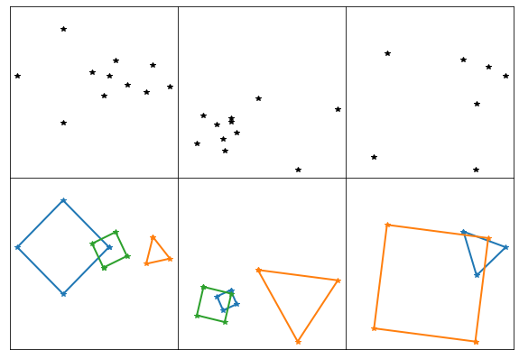
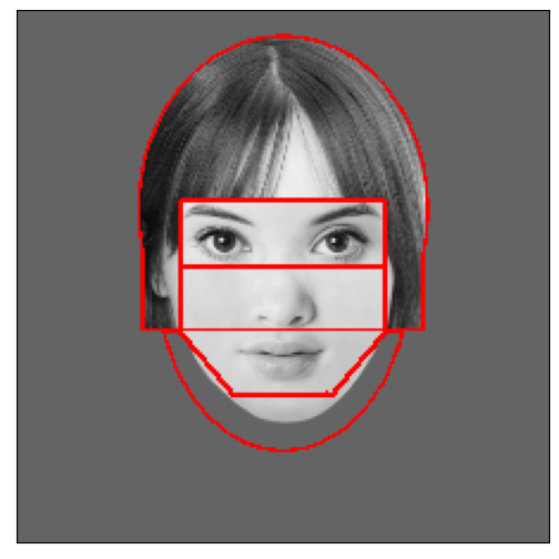
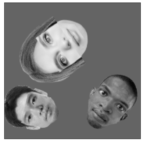
(a)	(b)	(c)

Figure 1: (a) Scenes composed of 2D points (upper figures) and their corresponding objects (lower figures). (b) A synthetic face. The red lines indicate the areas of the 5 part types (i.e. hair, eyes, nose, mouth and jaw). (c) Example scene with 3 randomly transformed faces.

2 Overview

Consider images of a set of objects in different poses, such as images of handwritten digits, faces, or geometric shapes in 2D or 3D. An object can be defined as an instantiation of a specific model object (or template) along with a particular pose (or geometric transformation). Furthermore, objects, and thus templates, are decomposed in parts, which are the basic elements that comprise the objects. For example, faces can be decomposed into parts (e.g. mouth, nose etc.), or a geometric shape can be decomposed into vertices. These parts can have internal variability, (e.g. eyes open or shut).

More formally, let $T=\{T_{k}\}_{k=1}^{K}$ be the set of $K$ templates that are used to generate a scene. Each template $T_{k}=\{{\mathbf{p}}_{n}\}_{n=1}^{N_{k}}$ is composed of $N_{k}$ parts ${\mathbf{p}}_{n}$. We assume that scenes can only be generated using the available templates. Furthermore, every scene can present a different configuration of objects, with some objects missing in some scenes. For example, in scenes that could potentially contain all digits from 0 to 9 once, and if only the digits 2 and 5 are in the image, we consider that the other digits are missing. If all the templates were employed in the scene, then the number of observed parts $M$ is equal to the sum of all the parts of all the templates $N=\sum_{k=1}^{K}N_{k}$.

Each observed template $T_{k}$ in a scene is then transformed by an independent transformation ${\mathbf{y}}_{k}$, different for each template, generating a set of transformed parts $X_{k}=\{{\mathbf{x}}_{n}\}_{n=1}^{N_{k}}$

$$T_{k}\stackrel{{\scriptstyle{\mathbf{y}}_{k}}}{{\rightarrow}}X_{k}.$$ (1)

The transformation ${\mathbf{y}}_{k}$ includes both the geometric transformation of the template, and also the appearance variability in the parts.

In this paper we assume that we are given a scene $X=\{{\mathbf{x}}_{m}\}_{m=1}^{M}$ composed of $M$ observed parts coming from multiple templates. (For example, the Part Capsule Autoencoder (PCAE) of Kosiorek et al., (2019) outputs a set of parts.) The inference problem for $X$ involves a number of different tasks. We need to determine which objects from the set of templates were employed to generate the scene. Also, we need to infer what transformation ${\mathbf{y}}_{k}$ was applied to each template to generate the objects. This allows us to infer the correspondences between the template parts and the scene parts.

We demonstrate our method on “constellations” data as shown in Fig. 1(a), and data containing multiple faces (Fig. 1(c)). In the constellations data, the real generators are triangle and square objects, but only their vertices are provided in the data. The faces data is generated from the parts-based model of faces shown in Fig. 1(b) and described in sec. 8.2.1.

3 A Generative Capsules Model (GCM)

We propose a generative model to describe the problem. Consider a template (or model) $T_{k}$ for the $k$th object. $T_{k}$ is composed of $N_{k}$ parts $\{{\mathbf{p}}_{n}\}_{n=1}^{N_{k}}$. Each part ${\mathbf{p}}_{n}$ is described in its reference frame by its geometry ${\mathbf{p}}^{g}_{n}$ and its appearance ${\mathbf{p}}^{a}_{n}$. Each object also has associated latent variables ${\mathbf{y}}_{k}$ which transform from the reference frame to the image frame, so ${\mathbf{y}}_{k}$ is split into geometric variables ${\mathbf{y}}^{g}_{k}$ and appearance variables ${\mathbf{y}}^{a}_{k}$.

Geometric transformations:

Here we consider 2D templates and a similarity transformation (translation, rotation and scaling) for each object, but this can be readily extended to allow 3D templates and a scene-to-viewer camera transformation. We assume that ${\mathbf{p}}_{n}^{g}$ contains the $x$ and $y$ locations of the part, and also its size $s_{n}$ and orientation $\phi_{n}$ relative to the reference frame. The size and orientation are represented as the projected size of the part onto the $x$ and $y$ axes, as this allows us to use linear algebra to express the transformations (see below). Thus ${\mathbf{p}}_{n}^{g}=(p^{g}_{nx},p^{g}_{ny},s_{n}\cos\phi_{n},s_{n}\sin\phi_{n})^{T}$.

Consider a template with parts ${\mathbf{p}}^{g}_{n}$ for $n=1,\ldots,N_{k}$ that we wish to scale by a factor $s$, rotate through with a clockwise rotation angle $\theta$ and translate by $(t_{x},t_{y})$. We obtain a transformed object with geometric observations for the $n$th part ${\mathbf{x}}^{g}_{n}=(x^{g}_{nx},x^{g}_{ny},x^{g}_{nc},x^{g}_{ns})$, where the $c$ and $s$ subscripts denote the projections of the scaled and rotated part onto the $x$ and $y$ axes respectively ($c$ and $s$ are mnemonic for cosine and sine).

For each part in the template, the geometric transformation works as follows:

$$\begin{pmatrix}x_{nx}\\ x_{ny}\\ x_{nc}\\ x_{ns}\end{pmatrix}=\begin{pmatrix}1&0&p_{nx}&p_{ny}\\ 0&1&p_{ny}&-p_{nx}\\ 0&0&s_{n}\cos\phi_{n}&-s_{n}\sin\phi_{n}\\ 0&0&s_{n}\sin\phi_{n}&s_{n}\cos\phi_{n}\\ \end{pmatrix}\begin{pmatrix}t_{x}\\ t_{y}\\ s\cos{\theta}\\ s\sin{\theta}\end{pmatrix}.$$ (2)

Decoding the third equation, we see that $x_{nc}=s_{n}s\cos\phi_{n}\cos\theta-s_{n}s\sin\phi_{n}\sin\theta=s_{n}s\cos(\phi_{n}+\theta)$ using standard trigonometric identities. The $x_{ns}$ equation is derived similarly. We shorten eq. 2 to ${\mathbf{x}}^{g}_{n}=F^{g}_{kn}{\mathbf{y}}^{g}_{k}$, where ${\mathbf{y}}^{g}_{k}$ is the ${\mathbb{R}}^{4}$ column vector, and $F^{g}_{kn}\in{\mathbb{R}}^{4\times 4}$ is the matrix to its left. Allowing Gaussian observation noise with precision $\lambda$ we obtain

$$p({\mathbf{x}}^{g}_{n}|T_{k},{\mathbf{y}}^{g}_{k})\sim N\left({\mathbf{x}}^{g}_{n}|F^{g}_{kn}{\mathbf{y}}^{g}_{k},\lambda^{-1}I\right).$$ (3)

The prior distribution over similarity transformations ${\mathbf{y}}^{g}_{k}$ is modelled with a ${\mathbb{R}}^{4}$ Gaussian distribution with mean ${\bm{\mu}}^{g}_{0}$ and covariance matrix $D^{g}_{0}$:

$$p(Y^{g})=\prod_{k=1}^{K}N({\mathbf{y}}^{g}_{k}|{\bm{\mu}}^{g}_{0},D^{g}_{0}),$$ (4)

where $Y^{g}$ denotes the set $\{{\mathbf{y}}^{g}_{k}\}_{k=1}^{K}$. Notice that modelling ${\mathbf{y}}^{g}_{k}$ with a Gaussian distribution implies that we are modelling the translation $(t_{x},t_{y})$ in ${\mathbb{R}}^{2}$ with a Gaussian distribution. If ${\bm{\mu}}^{g}_{0}=\mathbf{0}$ and $D^{g}_{0}=I_{4}$ then $s^{2}=(y^{g}_{k3})^{2}+(y^{g}_{k4})^{2}$ has a $\chi^{2}_{2}$ distribution, and $\theta=\arctan{{y^{g}_{k4}}/{y^{g}_{k3}}}$ is uniformly distributed in its range $[-\pi,\pi]$ by symmetry. For more complex linear transformations (e.g. an affine transformation), we need only to increase the dimension of ${\mathbf{y}}^{g}_{k}$ and change the form of $F^{g}_{kn}$, but the generative model in (4) would remain the same. For the 3D case, note that Basri, (1996) has shown that every affine projection of an object represents some uncalibrated paraperspective projection of the object.

Appearance transformations:

The appearance ${\mathbf{x}}_{n}^{a}$ of part $n$ in the image depends on ${\mathbf{y}}^{a}_{k}$. For our faces data, ${\mathbf{y}}^{a}_{k}$ is a vector latent variable which models the co-variation of the appearance of the parts via a linear (factor analysis) model; see sec. 8.2.1 for a fuller description. Hence

$$p({\mathbf{x}}^{a}_{n}|T_{k},{\mathbf{y}}_{k})\sim N\left({\mathbf{x}}^{a}_{n}|F^{a}_{kn}{\mathbf{y}}^{a}_{k}+\bm{m}_{kn}^{a},D^{a}_{kn}\right),$$ (5)

where $F^{a}_{kn}$ maps from ${\mathbf{y}}^{a}_{k}$ to the predicted appearance features in the image, $D^{a}_{kn}$ is a diagonal matrix of variances and $\bm{m}_{kn}^{a}$ allows for the appearance features to have a non-zero mean. The dimensionality of the $n$th part of the $k$th template is $d_{kn}$. The prior for ${\mathbf{y}}^{a}_{k}$ is taken to be a standard Gaussian, i.e. $N(\mathbf{0},I)$. Combining (4) and the prior for ${\mathbf{y}}^{a}_{k}$, we have that $p({\mathbf{y}}_{k})=N({\bm{\mu}}_{0},D_{0})$, where ${\bm{\mu}}_{0}$ stacks ${\bm{\mu}}^{g}_{0}$ and $\mathbf{0}$ from the appearance, and $D_{0}$ is a diagonal matrix with blocks $D^{g}_{0}$ and $I$.

Joint distribution:

Let $z_{mnk}\in\{0,1\}$ indicate whether observed part ${\mathbf{x}}_{m}$ matches to part $n$ of object $k$. The set of these match variables is denoted by $Z$. Every observation $m$ belongs uniquely to a tuple $(k,n)$, or in other words, a point ${\mathbf{x}}_{m}$ belongs uniquely to the part defined by ${\mathbf{y}}_{k}$ acting on the template matrix $F_{kn}$. The opposite is also partially true; every tuple $(k,n)$ belongs uniquely to a point $m$, or it is unassigned if part $n$ of template $k$ is missing in the scene.

The joint distribution of the variables in the model is given by

$$p(X,Y,Z)=p(X|Y,Z)p(Y)p(Z),$$ (6)

where $p(X|Y,Z)$ is a Gaussian mixture model explaining how the points in a scene were generated from the templates

$$p(X|Y,Z)=\prod_{m=1}^{M}\prod_{k=1}^{K}\prod_{n=1}^{N_{k}}N\left({\mathbf{x}}_{m}|F_{kn}{\mathbf{y}}_{k}+\bm{m}_{kn},D_{kn}\right)^{z_{mnk}},$$ (7)

where $D_{kn}$ consists of the diagonal matrices $\lambda^{-1}I$ and $D^{a}_{kn}$ and $\bm{m}_{kn}$ consists of a zero vector for the geometric features stacked on top of the mean for the appearance features $\bm{m}^{a}_{kn}$. Note that $F_{kn}$ has blocks of zeros so that ${\mathbf{x}}^{g}_{m}$ does not depend on ${\mathbf{y}}^{a}_{k}$, and ${\mathbf{x}}^{a}_{m}$ does not depend on ${\mathbf{y}}^{g}_{k}$.

Annealing parameter:

During inference, where the model is fitted to data, it is useful to modify the covariance matrix $D_{kn}$ to $\beta^{-1}D_{kn}$, where $\beta$ is a parameter $<1$. The effect of this is to inflate the variances in $D_{kn}$, allowing greater uncertainty in the inferred matches early on in the fitting process, as used, e.g. in Revow et al., (1996). $\beta$ is increased according to an annealing schedule during the fitting.

Match distribution $p(Z)$:

In a standard Gaussian mixture model, the assignment matrix $Z$ is characterized by a Categorical distribution, where each point ${\mathbf{x}}_{m}$ is assigned to one part

$$p(Z)=\prod_{m=1}^{M}\text{Cat}({\mathbf{z}}_{m}|{\bm{\pi}}),$$ (8)

with ${\mathbf{z}}_{m}$ being a 0/1 vector with only one 1, and ${\bm{\pi}}$ being the probability vector for each tuple $(k,n)$. However, the optimal solution to our problem occurs when each part of a template belongs uniquely to one observed part in a scene. This means that $Z$ should be a permutation matrix, where each point $m$ is assigned to a tuple $(k,n)$ and vice versa. Notice that a permutation matrix is a square matrix, so if $M\leq N$, we add dummy rows to $Z$, which are assigned to missing points in the scene.

The set of permutation matrices of dimension $N$ is a discrete set containing $N!$ permutation matrices. A discrete prior over permutation matrices assigns each valid matrix $Z_{i}$ a probability $\pi_{i}$:

$$p_{perm}(Z)=\sum_{i=1}^{N!}\pi_{i}\;I[Z=Z_{i}]$$ (9)

with $\sum_{i=1}^{N!}\pi_{i}=1$ and $I[Z=Z_{i}]$ being the indicator function, equal to $1$ if $Z=Z_{i}$ and $0$ otherwise.

The number of possible permutation matrices increases as $N!$, which makes exact inference over permutations intractable, except for very small $N$. An interesting property of $p_{perm}(Z)$ is that its first moment ${\mathbb{E}}_{p_{perm}}[Z]$ is a doubly-stochastic (DS) matrix, a matrix of elements in $[0,1]$ whose rows and columns sum to 1. We propose to relax $p_{perm}(Z)$ to a distribution $p_{DS}(Z)$ that is characterized by the doubly-stochastic matrix $A$ with elements $a_{mnk}$, such that ${\mathbb{E}}_{p_{DS}}[Z]=A$:

$$p_{DS}(Z)=\prod_{m=1}^{N}\prod_{k=1}^{K}\prod_{n=1}^{N_{k}}a_{mnk}^{z_{mnk}}.$$ (10)

$A$ is fully characterized by $(N-1)^{2}$ elements. In the absence of any prior knowledge of the affinities, a uniform prior over $Z$ with $a_{mnk}=\frac{1}{N}$ can be used. However, note that $p_{DS}$ can also represent a particular permutation matrix $Z_{i}$ by setting the appropriate entries of $A$ to 0 or 1, and indeed we would expect this to occur during variational inference (see sec. 4) when the model converges to a correct solution.

Related models:

Our model for a single object has both geometric and appearance variability (see eqs. 3 and 5). A similar model but with geometric features only was developed by Revow et al., (1996). Fergus et al., (2003) described a “constellation of parts” model, that used a joint Gaussian model for locations of the parts, and an image-patch model for each part appearance. However, the appearance model was a single Gaussian per part, without the correlations between parts afforded by the factor analysis model. This model was applied to images of single (foreground) objects, summing out over possible assignments $Z$. Rao and Ballard, (1999) developed a hierarchical factor analysis model, but used it to model extended edges in natural image patches rather than correlations between the parts of an object. See sec. 7 for further discussion of parts-based models.

Hierarchical modelling:

above we have described a two-layer model with part-object relations. This can of course be extended to a deeper hierarchy; for example we would expect to find relationships between the objects in a scene, such as the relationships between a dining table and the dining chairs, or between a bed and its associated nightstand(s). Such scene-level relationships can be formulated in terms of graphical models for the groups of objects. We believe the most difficult aspect is handling the assignment $Z$ between model parts and observed parts (as covered in this paper), and that inference in the graphical model above is fairly standard, and is left for future work.

4 Variational Inference

Variational inference for the above model can be derived similarly to the Gaussian Mixture model case (Bishop,, 2006, Sec. 10.1). The variational distribution under the mean field assumption is given by $q(Z,Y)=q(Z)q(Y)$, The evidence lower error bound (ELBO) for this model is derived in Appendix A. Optimizing the ELBO with respect to either $q(Z)$ or $q(Y)$, the optimal solutions can be expressed as

$$\log{q(Z)} \propto {\mathbb{E}}_{q(Y)}[\log{p(X,Y,Z)}],$$ (11)

$$\log{q(Y)} \propto {\mathbb{E}}_{q(Z)}[\log{p(X,Y,Z)}].$$ (12)

These alternating updates of $q(Y)$ and $q(Z)$ carry out routing-by-agreement.

For $q(Z)$ we obtain an expression with the same form as the prior in (10)

$$q(Z)\propto\prod_{m=1}^{N}\prod_{k=1}^{K}\prod_{n=1}^{N_{k}}\rho_{mnk}^{z_{mnk}},$$ (13)

where $\rho_{mnk}$ represents the unnormalized probability of point $m$ being assigned to tuple $(k,n)$ and vice versa. These unnormalized probabilities have a different form depending on whether we are considering a point that appears in the scene ($m\leq M$)

$$\log{\rho_{mnk}}=\log{a_{mnk}}-\frac{1}{2}\log{|\beta^{-1}D_{kn}|}-\frac{d_{kn}}{2}\log{2\pi}-$$

$$\frac{\beta}{2}{\mathbb{E}}_{{\mathbf{y}}_{k}}[({\mathbf{x}}_{m}-F_{kn}{\mathbf{y}}_{k}-\bm{m}_{kn})^{T}D_{kn}^{-1}({\mathbf{x}}_{m}-F_{kn}{\mathbf{y}}_{k}-\bm{m}_{kn})],$$ (14)

or whether we are considering a dummy row of the prior ($m>M$),

$$\log{\rho_{mnk}} =\log{a_{mnk}}.$$ (15)

When a point is part of the scene (14), and thus $m\leq M$ the update of $\rho_{mnk}$ is similar to the Gaussian mixture model case. However, if a point is not part of the scene (15), and thus $m>M$ then the matrix is not updated and the returned value is the prior $a_{mnk}$. The expectation term in (14) is given by:

$${\mathbb{E}}_{{\mathbf{y}}_{k}}[({\mathbf{x}}_{m}-F_{kn}{\mathbf{y}}_{k}-\bm{m}_{kn})^{T}D_{kn}^{-1}({\mathbf{x}}_{m}-F_{kn}{\mathbf{y}}_{k}-\bm{m}_{kn})]=\\ ({\mathbf{x}}_{m}-F_{kn}{\bm{\mu}}_{k}-\bm{m}_{kn})^{T}D_{kn}^{-1}({\mathbf{x}}_{m}-F_{kn}{\bm{\mu}}_{k}-\bm{m}_{kn})+\text{trace}(F_{kn}^{T}D_{kn}^{-1}F_{kn}\Lambda_{k}^{-1}).$$ (16)

The normalized distribution $q(Z)$ becomes:

$$q(Z)=\prod_{m=1}^{N}\prod_{k=1}^{K}\prod_{n=1}^{N_{k}}r_{mnk}^{z_{mnk}},$$ (17)

where ${\mathbb{E}}_{q(Z)}[z_{mnk}]=r_{mnk}$. The elements $r_{mnk}$ of matrix $R$ represent the posterior probability of each point $m$ being uniquely assigned to the part-object tuple $(n,k)$ and vice-versa. This means that $R$ needs to be a DS matrix. This can be achieved by employing the Sinkhorn-Knopp algorithm (Sinkhorn and Knopp,, 1967) as given in Algorithm 1, which updates a square non-negative matrix by normalizing the rows and columns alternately until the resulting matrix becomes doubly stochastic.

The use of the Sinkhorn-Knopp algorithm for approximating matching problems has also been described by Powell and Smith, (2019) and Mena et al., (2020), but note that in our case we also need to alternate with inference for $q(Y)$.

Algorithm 1 Sinkhorn-Knopp algorithm, taking as input a square non-negative matrix $M$

1:procedure SinkhornKnopp($M$)

2:     while $M$ not doubly stochastic do

3:         Normalize rows of $M$: $m_{ij}=\frac{m_{ij}}{\sum_{j}m_{ij}}$, $\forall{i}$

4:         Normalize columns of $M$: $m_{ij}=\frac{m_{ij}}{\sum_{i}m_{ij}}$, $\forall{j}$      return $M$

Furthermore, the optimal solution to the assignment problem occurs when $R$ is a permutation matrix itself. When this happens we exactly recover a discrete posterior (with the same form as (9)) over permutation matrices where one of them has probability one, with the others being zero.

The distribution for $q(Y)$ is a Gaussian with

$$q(Y) =\prod_{k=1}^{K}N({\mathbf{y}}_{k}|{\bm{\mu}}_{k},\Lambda_{k}^{-1}),$$ (18)

$$\Lambda_{k} =D^{-1}_{0}+\beta\sum^{M}_{m}\sum^{N_{k}}_{n}r_{mnk}F_{kn}^{T}D_{kn}^{-1}F_{kn},$$ (19)

$${\bm{\mu}}_{k} =\Lambda_{k}^{-1}\left[D_{0}{\bm{\mu}}_{0}+\beta\sum^{M}_{m}\sum^{N_{k}}_{n}r_{mnk}F_{kn}^{T}D_{kn}^{-1}({\mathbf{x}}_{m}-\bm{m}_{kn})\right],$$ (20)

where the updates for both $\Lambda_{k}$ and ${\bm{\mu}}_{k}$ depend explicitly on the annealing parameter $\beta$ and the templates employed in the model. Note that the prediction from datapoint $m$ to the mean of ${\mathbf{y}}_{k}$ depends on $r_{mnk}F_{kn}^{T}D^{-1}_{kn}({\mathbf{x}}_{m}-\bm{m}_{kn})$, i.e. a weighted sum of the predictions of each part $n$ with weights $r_{mnk}$. These expressions remain the same when considering a Gaussian mixture prior such as (8).

Algorithm 2 summarizes the inference procedure for this model.

Algorithm 2 Variational Inference

1:Initialize $\beta$, $\beta_{max}$ and $R\sim U[0,1]^{N\times N}$, $\forall m,n,k$

2:$R=\text{SinkhornKnopp}(R)$

3:while not converged do

4:     Update $\Lambda_{k}$ (19), $\forall k$

5:     Update ${\bm{\mu}}_{k}$ (20), $\forall k$

6:     Update $\log{\rho_{mnk}}$ (14)(15), $\forall m,n,k$

7:     Update $R=\text{SinkhornKnopp}(\rho)$

8:     if ELBO has converged then

9:         if $\beta<\beta_{max}$ then

10:              Anneal $\beta$

11:         else

12:              converged = True               return $R,\{{\bm{\mu}}_{k},\Lambda_{k}\}$

4.1 Comparison with other objective functions

In Hinton et al., (2018) an objective function $cost^{h}_{k}$ is defined (their eq. 1) which considers inference for the pose of a higher-level capsule $k$ on pose dimension $h$. Translating to our notation, $cost^{h}_{k}$ combines the predictions ${\mathbf{v}}_{mk}$ from each datapoint $m$ for capsule $k$ as $cost^{h}_{k}=\sum_{m}r_{mk}\ln P^{h}_{m|k}$, where $P^{h}_{m|k}$ is a Gaussian, and $r_{mk}$ is the “routing softmax assignment” between $m$ and $k$. It is interesting to compare this with our equation (20). Firstly, note that the vote of ${\mathbf{x}}_{m}$ to part $n$ in object $k$ is given explicitly by $\beta\Lambda_{k}^{-1}F^{T}_{kn}D^{-1}_{kn}({\mathbf{x}}_{m}-\bm{m}_{kn}),$ i.e. we do not require the introduction of an independent voting mechanism, this falls out directly from the inference. Secondly, note that our $R$ must keep track not only of assignments to objects, but also to parts of the objects. In our experiments with the constellations data each observed part could match any object/part combination of the models, so this is necessary. For the faces data, the observed parts are of identifiable type (e.g. nose, mouth), so in this case they only need to vote for the object. In contrast to Hinton et al., (2018), our inference scheme is derived from variational inference on the generative model for $X$, rather than introducing an ad hoc objective function that corresponds to a clustering in ${\mathbf{y}}$-space.

De Sousa Ribeiro et al., 2020a develop a variational Bayes extension of the model of Hinton et al., (2018). They write down a mixture model in ${\mathbf{y}}$-space where the “datapoints” are the votes ${\mathbf{v}}_{mk}$, and use Bayesian priors for the mixing proportions, and for the means and covariance matrices of the components. This can improve training stability, e.g. by reducing the problem of variance-collapse where a capsule claims sole custody of of a datapoint. However, this is still a model for clustering in ${\mathbf{y}}$-space, and not a generative model for $X$.

The specialization of the SCAE method of Kosiorek et al., (2019) to constellation data is called the “constellation capsule autoencoder (CCAE)” and discussed in their sec. 2.1. Under their equation 5, we have that

$$p({\mathbf{x}}_{1:M})=\prod_{m=1}^{M}\sum_{k=1}^{K}\sum_{n=1}^{N}\frac{a_{k}a_{k,n}}{\sum_{i}a_{i}\sum_{j}a_{ij}}N({\mathbf{x}}_{m}|\mu_{k,n},\lambda_{k,n}),$$ (21)

where $a_{k}\in[0,1]$ is the presence probability of capsule $k$, $a_{k,n}\in[0,1]$ is the conditional probability that a given candidate part $n$ exists, and $\mu_{k,n}$ is the predicted location of part $k,n$. The $a_{k}$s are predicted by the network $h^{\mathrm{caps}}$, while the $a_{k,n}$s and $\mu_{k,n}$s are produced by separate networks $h_{k}^{\mathrm{part}}$ for each part $k$.

We note that (21) provides an autoencoder style reconstructive likelihood for ${\mathbf{x}}_{1:M}$, as the $a$’s and $\mu$’s depend on the data. To handle the arbitrary number of datapoints $M$, the network $h^{\mathrm{caps}}$ employs a Set Transformer architecture (Lee et al.,, 2019). In comparison to our iterative variational inference, the CCAE is a “one shot” inference mechanism. This may be seen as an advantage, but in scenes with overlapping objects, humans may perform reasoning like “if that point is one of the vertices of a square, then this other point needs to be explained by a different object” etc, and it may be rather optimistic to believe this can be done in a simple forward pass. Also, the CCAE cannot exploit prior knowledge of the geometry of the objects, as it relies on an opaque network $h^{\mathrm{caps}}$ which requires extensive training.

Algorithm 3 RANSAC approach

1:$T$: $K$ templates of the scene

2:$B_{k}$: base matrix for template $T_{k}$

3:$X$: $M$ points of the scene

4:$out=[]$

5:for ${\mathbf{x}}_{i}\in X$ do

6:     for ${\mathbf{x}}_{j}\in X\setminus x_{i}$ do

7:         ${\mathbf{x}}_{ij}=\text{Vectorize}({\mathbf{x}}_{i},{\mathbf{x}}_{j})$

8:         for $k=1:K$ do

9:              $\hat{{\mathbf{y}}}_{k}=B_{k}^{-1}{\mathbf{x}}_{ij}$

10:              $T_{k}\xrightarrow{\hat{{\mathbf{y}}}_{k}}\hat{X}_{k}$

11:              if  SubsetMatch($\hat{X}_{k},X)$ then

12:                  Add $(T_{k},\hat{{\mathbf{y}}}_{k},\hat{X}_{k})$ to $out$                             return $out$

5 A RANSAC Approach to Inference

A radical alternative to “routing by agreement” inference is to make use of a “random sample consensus” approach (RANSAC, Fischler and Bolles,, 1981), where a minimal number of parts are used in order to instantiate an object. The original RANSAC fitted just one object, but Sequential RANSAC (see, e.g., Torr, 1998; Vincent and Laganière, 2001) repeatedly removes the parts associated with a detected object and re-runs RANSAC, so as to detect all objects.

For the constellations problem, we can try matching any pair of points on one of the templates to every possible pair of $M(M-1)$ points in the scene. The key insight is that a pair of known points is sufficient to estimate the 4-dimensional $\hat{{\mathbf{y}}}_{k}$ vector in the case of similarity transformations. Using the transformation $\hat{{\mathbf{y}}}_{k}$, we can then predict the location of the remaining parts of the template, and check if these are actually present. If so, this provides evidence for the existence of $T_{k}$ and $\hat{{\mathbf{y}}}_{k}$. After considering the $M(M-1)$ subsets, the algorithm then combines the identified instantiations to give an overall explanation of the scene.

More details of the RANSAC approach are given in Algorithm 3. Assume we have chosen parts $n_{1}$ and $n_{2}$ as the basis for object $k$, and that we have selected datapoints ${\mathbf{x}}_{i}$ and ${\mathbf{x}}_{j}$ as their hypothesized counterparts in the image. Let ${\mathbf{x}}_{ij}$ be the vector obtained by stacking ${\mathbf{x}}_{i}$ and ${\mathbf{x}}_{j}$, and $B_{k}$ be the $4\times 4$ square matrix obtained by stacking $F_{kn_{1}}$ and $F_{kn_{2}}$. Then $\hat{{\mathbf{y}}}_{k}=B_{k}^{-1}{\mathbf{x}}_{ij}$. Finally, $\text{SubsetMatch}(\hat{X}_{k},X)$ selects those points in $X_{k}$ that are close to $X$ with a given tolerance and add them to the output. Among them, the solution is given by the one that minimizes $\sum_{n=1}^{N_{k}}(\hat{x}_{nk}-x_{nk})^{2}$.

The above algorithm chooses a specific basis for each object, but one can consider all possible bases for each object. It is then efficient to use a hash table to store the predictions for each part, as used in Geometric Hashing (Wolfson and Rigoutsos,, 1997). Geometric Hashing is traditionally employed in computer vision to match geometric features against previously defined models of such features. This technique works well with partially occluded objects, and is computationally efficient if the basis dimension is low.

For the faces data, each part has location, scale and orientation information, so a single part is sufficient to instantiate the whole object geometrically. For the appearance, we follow the procedure for inference in a factor analysis model with missing data, as given in Williams et al., (2019), to predict ${\mathbf{y}}^{a}_{k}$ given the appearance of the single part.

It is interesting to compare the RANSAC and routing-by-agreement approaches to identifying objects. In RANSAC a minimal basis is chosen so as to instantiate the object, which is then verified by finding the remaining parts in the predicted locations. In contrast routing-by-agreement makes predictions from all of the observed parts, and then seeks to adjust the $R$ matrix so as to cluster these predictions into coherent objects. This is generally an iterative process, although the SCAE autoencoder architecture is “one shot”.

6 Related Work

The origins of capsule networks (including the name “capsule”) can be traced back at least as far as the work of Hinton et al., (2011) on Transforming Auto-encoders. Capsules were further developed in Sabour et al., (2017). Above we have already discussed later work by Hinton and co-workers, including Hinton et al., (2018), Kosiorek et al., (2019), and also De Sousa Ribeiro et al., 2020a .

The paper by De Sousa Ribeiro et al., (2022) provides a thorough survey of capsules. Below we highlight a few papers on capsules; for example Li and Zhu, (2019) develop a capsule Restricted Boltzmann Machine (RBM). This generative model contains a number of capsules, each having a binary existence variable and a vector of capsule variables similar to our ${\mathbf{y}}_{k}$. However, these capsule variables are not used to model geometric transformations (the key idea behind capsule networks), but instead to handle appearance variability of the parts.

Both Li et al., (2020) and Smith et al., (2021) propose a layered directed generative model. These both make use of the "single parent constraint", where a capsule in a layer can be connected to only one capsule (its parent) in the layer above. Such tree-structured relationships are similar to those studied in Hinton et al., (2000) and Storkey and Williams, (2003). Like Li and Zhu, (2019), Li et al., (2020) do not explicitly consider modelling geometric transformations with their network. This aspect is explicit in Smith et al., (2021), where their capsule variables (similar to our ${\mathbf{y}}_{k}$s) do model pose, but not appearance variability.

However, most importantly, these recent capsule models do not properly handle the fact that the input to a capsule should be a set of parts; instead in their work the first layer capsules that interact with the input image model specific location-dependent features/templates in the image, and their second layer capsules have interactions with the specific first layer capsules (e.g. the fixed affinity $\rho^{k}_{ij}$ of Smith et al., (2021) parent $i$ in layer $k$ for child $j$). But if we consider a second-layer capsule that is, for example, detecting the conjunction of the 3 strokes comprising a letter “A”, then at different translations, scales and rotations of the A it will need to connect to different image level stroke features, so these connection affinities must depend on transformation variables of the parent. This point is illustrated in Fig. 2 of sec. 7 for the PCAE parts, and is also made in sec. 5.4 of Smith et al., (2021), where it is shown that the parts decomposition used of a digit image is not stable with respect to rotation of the digit.

(a)
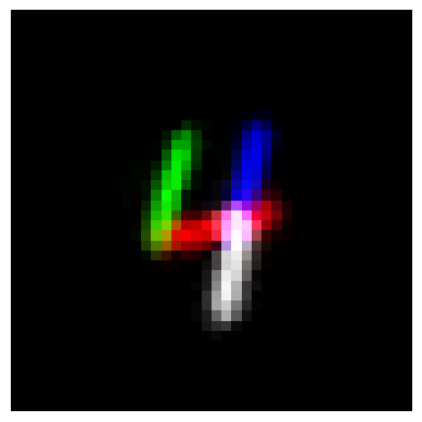
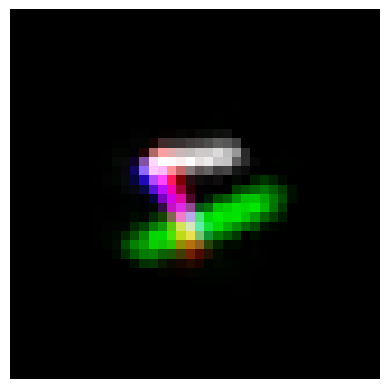
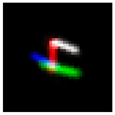
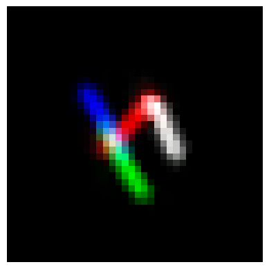
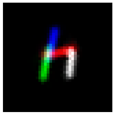
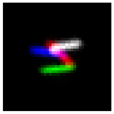
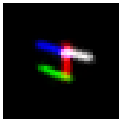
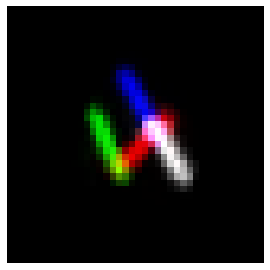
(b)
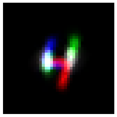
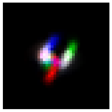
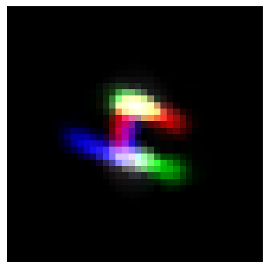
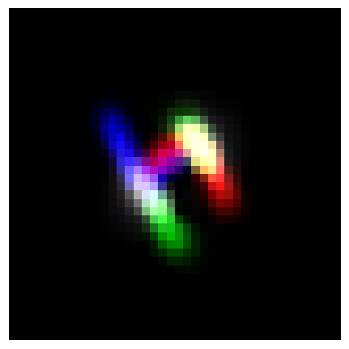
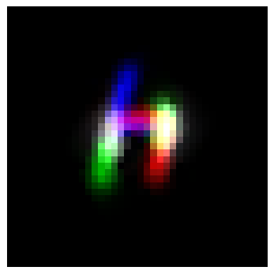
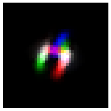
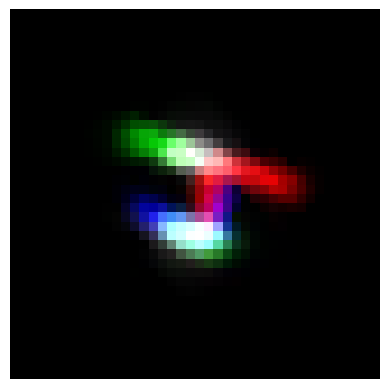
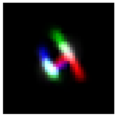
	$0^{\circ}$	$45^{\circ}$	$90^{\circ}$	$135^{\circ}$	$180^{\circ}$	$225^{\circ}$	$270^{\circ}$	$315^{\circ}$

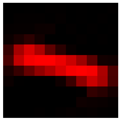
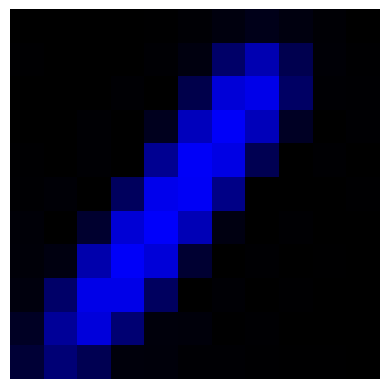
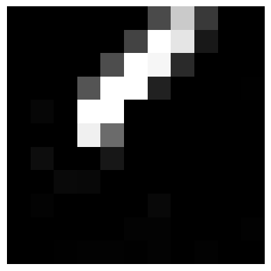
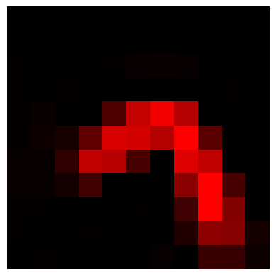
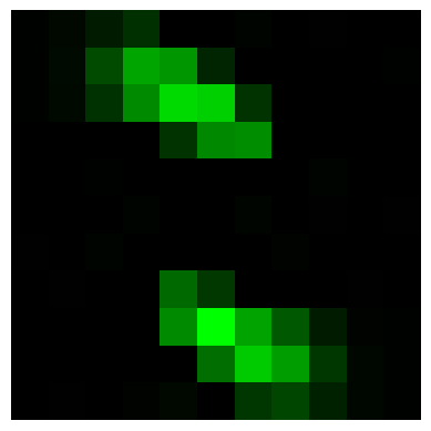
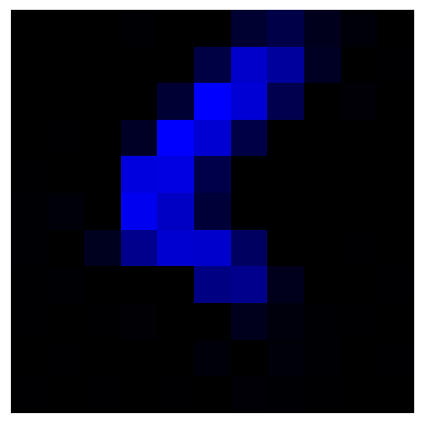
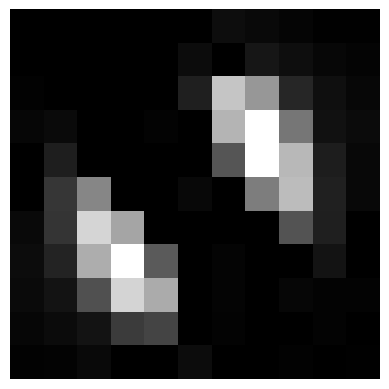
		part-set-a					part-set-b

Figure 2: PCAE-based reconstruction for different angles of rotation of the input scenes. Row (a) corresponds to reconstructions with the learned part-set-a and row (b) reconstructions with the learned part-set-b. The parts are $11\times 11$ pixels, and the images in rows (a) and (b) are $40\times 40$.

7 Learning Generative Capsule Models

Above we have assumed that the models are given, i.e. that $F_{kn}$ and $\bm{m}_{kn}$ are known for each part $n$ and model $k$. One advantage of the interpretable nature of the GCM is that one can use a “curriculum learning” approach (Bengio et al.,, 2009), where individual models can first be learned, and then composed together for inference in more complex situations.

For a given object, a key issue is the learning of the decomposition into parts. For the constellations data this is not an issue as the points (i.e. parts) are given, but for image data it must be addressed. An important issue is the degree of flexibility of each part—is it simply a fixed template, or are there internal degrees of flexibility? An example of the former is non-negative matrix factorization (NMF) (Lee and Seung,, 1999), where, for example, aligned images of faces were decomposed into non-negative basis functions (parts) that were combined with non-negative coefficients. An example of a richer parts-based model is by Ross and Zemel, (2006), who developed “multiple cause factor analysis” (MCFA) and applied it to faces, to learn the regions governed by each part and the variability within each part. This work was also carried out on aligned, vertically oriented face images, so it was not necessary to factor out geometric transformations. For our work on faces, we made use of the parts-based model from the “PhotoFitMe” work described in section 8.2.1. This provided a ready-made parts decomposition, but we learned a factor analysis model on top to model the correlations between the parts.

Kosiorek et al., (2019) developed a Part Capsule Autoencoder (PCAE) to learn parts from images, and applied it to MNIST images. Each PCAE part is a template which can undergo an affine transformation, and it has "special features" that were used to encode the colour of the part. If the overall model is to be equivariant to geometric transformations, it is vital that the input part decomposition is stable to such variation, otherwise the model is building on shaky foundations. However, we have observed that the parts detected by PCAE are not equivariant to rotation. Figure 2 shows that the PCAE part decompositions inferred for a digit 4 are not stable to different angles of rotation: notice e.g. in panel (a) how the part coloured white maps to different parts of the 4 for $45^{\circ}$-$180^{\circ}$ and $225^{\circ}$-$0^{\circ}$. The details of this experiment are described in Appendix D.

As identified above, a strength of the GCM is that individual models can first be learned, before moving on to more complex situations. We can start with an initial guess for the object configuration, which can be chosen as one of the noisy configurations from the training set. We then run variational expectation maximization (variational EM; see sec. 6.2 in Jordan et al., 1999). In the E-step, variational inference is run as in sec. 4 with this model to infer the ${\mathbf{y}}$ and $Z$ variables on each training example. In the M-step, the variatonal distributions determined in the E-step are held fixed, and the locations of the template points are updated so as to increase the ELBO, summed over the training cases. Details of this update are given in Appendix B for the constellations dataset, and experimental results are given in sec. 8.1.3.

8 Experiments and Results

We first provide experimental details and results for inference and learning for the constellations data in sec. 8.1, and then give experimental details and results for the faces data in sec. 8.2.

8.1 Constellations: experiments and results

Below we provide details of the data generators, inference methods and evaluation criteria for the constellations data in sec. 8.1.1, present results for inference on the constellations data in sec. 8.1.2, and for learning constellation models in sec. 8.1.3.

8.1.1 Constellations experiments

In order to allow fair comparisons, we use the same dataset generator for geometric shapes employed by Kosiorek et al., (2019). We create a dataset of scenes, where each scene consists of a set of 2D points, generated from different geometric shapes. The possible geometric shapes (templates) are a square and an isosceles triangle, with parts being represented by the 2D coordinates of the vertices. We use the same dimensions for the templates as used by Kosiorek et al., (2019), side 2 for the square, and base and height 2 for the triangle. All templates are centered at $(0,0)$. In every scene there are at most two squares and one triangle, so $N=11$. Each shape is transformed with a random transformation to create a scene of 2D points given by the object parts. To match the evaluation of Kosiorek et al., (2019), all scenes are normalized so as the points lie in $[-1,1]$ on both dimensions. When creating the scene, we select randomly (with probability 0.5) whether an object is going to be present or not, but delete empty scenes. A test set used for evaluation is comprised of 450-460 non-empty scenes, based on 512 draws.

Additionally, we study how the methods compare when objects are created from noisy templates. We consider that the original templates used for the creation of the images are corrupted with Gaussian noise with standard deviation $\sigma$. Once the templates are corrupted with noise, a random transformation ${\mathbf{y}}_{k}$ is applied to obtain the object $X_{k}$ of the scene. As with the noise-free data, the objects are normalized to lie in [-1,1] on both dimensions.

The CCAE is trained by creating random batches of 128 scenes as described above and optimizing the objective function in (21). The authors run CCAE for $300K$ epochs, and when the parameters of the neural networks are trained, they use their model on the test dataset to generate an estimation of which points belong to which capsule, and where the estimated points are located in each scene.

The variational inference approach allows us to model scenes where the points are corrupted with some noise. The annealing parameter $\beta$ controls the level of noise allowed in the model. We use an annealing strategy to fit $\beta$, increasing it every time the ELBO has converged, up to a maximum value of $\beta_{max}=1$. We set the hyperparameters of the model to ${\bm{\mu}}^{g}_{0}=\mathbf{0}$, $D^{g}_{0}=I_{4}$, $\lambda=10^{4}$ and $a_{mnk}=\frac{1}{N}$. We run Algorithm 2 with 5 different random initializations of $R$ and select the solution with the best ELBO. Similarly to Kosiorek et al., (2019), we incorporate a sparsity constraint in our model, that forces every object to explain at least two parts. Once our algorithm has converged, for a given $k$ if any $r_{mnk}>0.9$ and $\sum_{m}\sum_{n}r_{mnk}<2$ it means that the model has converged to a solution where object $k$ is assigned to less than 2 parts. In these cases, we re-run Algorithm 2 with a new initialization of $R$. Notice that this is also related to the minimum basis size necessary in the RANSAC approach for the types of transformations that we are considering.

The implementation of SubsetMatch in Algorithm 3 considers all matches between the predicted and the scene points where the distance between them is less than $0.1$. Among them, it selects the matching with minimum distance between scene and predicted points.

For both the variational inference algorithm and the RANSAC algorithm, a training dataset is not necessary if we have prior knowledge of the target shapes. This contrasts with SCAE, which learns from whole scenes. If prior knowledge is not available, these shapes can be learned as described in sec. 7, and illustrated in sec. 8.1.3.

Unfortunately we do not have access to the code employed by Hinton et al., (2018), so we have been unable to make comparisons with it.

Evaluation: Three metrics are used to evaluate the performance of the different methods: variation of information (Meilă,, 2003), adjusted Rand index (Hubert and Arabie,, 1985) and segmentation accuracy (Kosiorek et al.,, 2019). They are based on partitions of the datapoints into those associated with each object, and those that are missing. Compared to standard clustering evaluation metrics, some modifications are needed to handle the missing objects. Details are provided in Appendix C. We also use an average scene accuracy metric, where a scene is correct if the method returns the full original scene, and is incorrect otherwise.

Table 1: Comparison between the different methods. For Segmentation Accuracy, Adjusted Rand Index and Scene Accuracy the higher the better. For Variation of Information the lower the better. Different levels of Gaussian noise with standard deviation $\sigma$ are considered.

Metric	Model	$\sigma$=0	$\sigma$=0.1	$\sigma$=0.25
	CCAE	0.828	0.754	0.623
Segmentation	GCM-GMM	0.753	0.757	0.744
Accuracy $\uparrow$	GCM-DS	0.899	0.882	0.785
	RANSAC	1	0.992	0.965
	CCAE	0.599	0.484	0.248
Adjusted	GCM-GMM	0.586	0.572	0.447
Rand Index$\uparrow$	GCM-DS	0.740	0.699	0.498
	RANSAC	1	0.979	0.914
	CCAE	0.481	0.689	0.988
Variation of	GCM-GMM	0.478	0.502	0.677
Information $\downarrow$	GCM-DS	0.299	0.359	0.659
	RANSAC	0	0.034	0.135
	CCAE	0.365	0.138	0.033
Scene	GCM-GMM	0.179	0.173	0.132
Accuracy $\uparrow$	GCM-DS	0.664	0.603	0.377
	RANSAC	1	0.961	0.843

8.1.2 Constellation Inference Experiments

In Table 1 we show a comparison between CCAE, the variational inference method with a Gaussian mixture prior (8) (GCM-GMM), with a DS prior over permutation matrices (9) (GCM-DS), and the RANSAC approach for scenes without noise and with noise levels of $\sigma=0.1,\;0.25$ . For GCM-GMM and GCM-DS we show the results where the initial $\beta=0.05$. The effect of different $\beta$ initializations is discussed below.

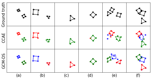
Figure 3: Reconstruction examples from CCAE and GCM-DS for noise-free data. The upper figures show the ground truth of the test images. The middle figures show the reconstruction and the capsule assignments (by colours) of CCAE. The lower figures show the reconstruction and the parts assignment of GCM-DS. Datapoints shown with a given colour are predicted to belong to the reconstructed object with the corresponding colour.

We see that GCM-DS improves over CCAE and GCM-GMM in all of the metrics, with GCM-GMM being comparable to CCAE. Interestingly, for the noise-free scenarios, the RANSAC method achieves a perfect score for all of the metrics. Since there is no noise on the observations and the method searches over all possible solutions of ${\mathbf{y}}_{k}$, it can find the correct solution for any configuration of geometric shapes in a scene. For the noisy scenarios, all the methods degrade as $\sigma$ increases. However, the relative performance between them remains the same, with RANSAC performing the best, followed by GCM-DS and then GCM-GMM.

Figure 3 shows some reconstruction examples from CCAE and GCM-DS for the noise-free scenario. In columns (a) and (b) we can see that CCAE recovers the correct parts assignments but the object reconstruction is inaccurate. In (a) one of the squares is reconstructed as a triangle, while in (b) the assignment between the reconstruction and the ground truth is not exact. For GCM-DS, if the parts are assigned to the ground truth properly, and there is no noise, then the reconstruction of the object is perfect. In column (c) all methods work well. In column (d), CCAE fits the square correctly (green), but adds an additional red point. In this case GCM-DS actually overlays two squares on top of each other. Both methods fail badly on column (e). Note that CCAE is not guaranteed to reconstruct an existing object correctly (square or triangle in this case). In column (f) we can see that CCAE fits an irregular quadrilateral (blue) to the assigned points, while GCM-DS obtains the correct fit. Additional examples for noisy cases with $\sigma=0.25$ are shown in Appendix E.

To assess the effect of in the initial value of $\beta$, we considered 6 values: 0.005, 0.01, 0.05, 0.1, 0.2, and 0.5. We found that GCM-DS is always better than CCAE and GCM-GMM. As the initial $\beta$ is increased, GCM-DS performs better across all the metrics. We found that the performance of GCM-DS and GCM-GMM degrades with $\beta>0.1$.

We conducted paired t-tests between CCAE and GCM-GMM, GCM-DS and RANSAC on the three clustering metrics for $\sigma=0$ and initial $\beta=0.05$. The differences between CCAE and GCM-DS are statistically significant with p-values less than $10^{-7}$, and between CCAE and RANSAC with p-values less than $10^{-28}$. For CCAE and GCM-GMM the differences are not statistically significant.

8.1.3 Learning Constellations

Making use of the interpretable nature of the GCM, we consider learning each template (triangle or square) individually from noisy data, with noise values of $\sigma=0,\,0.1,\,0.25$. (Note that the full dataset as generated contains 1/7 = 14% single triangles, and 28% single squares which can be selected simply based on the number of points.)

To compare the learned template to the ground-truth (GT), we have to bear in mind that the learned template could be a rotated version, as this will still be centered and have the correct scale. To remove this rotational degree of freedom, we compute the Procrustes rotation (see, e.g., Mardia et al., 1979, sec. 14.7) that best aligns them. After this, we can compute the standardized mean squared error (SMSE) $\frac{1}{N}\sum_{n=1}^{N}({\mathbf{p}}_{n}-{\mathbf{p}}^{GT}_{n})^{T}({\mathbf{p}}_{n}-{\mathbf{p}}^{GT}_{n})$.

We use $S=64$ examples to train each template, and use one random sample to seed the initial template (after translation, scaling and rotation). (In fact, for noise-free constellation data ($\sigma=0$), a single observed triangle or square configuration serves as a perfect template.) As $N$ is 3 or 4 in this case, we can use exact inference over permutations, rather than the variational approach. We initialized $\beta=0.01$ and increased it after each iteration by a factor of two, similarly to the annealing strategy utilized in Algorithm 2. The stopping criterion for the learning process was that the SMSE between two consecutive updates of the learned template should not be greater than $10^{-4}$.

For the triangle object, the SMSE of the learned template was $4.1\times 10^{-5}$ at $\sigma=0.1$, and $9.6\times 10^{-3}$ at $\sigma=0.25$. For the square object, the corresponding SMSEs were $1.8\times 10^{-4}$ and $2.1\times 10^{-2}$ respectively. Figure 4 shows example learned templates (after Procrustes rotation) compared to the GT templates. We see that with only $S=64$ examples, an accurate template can be learned for each object. As expected, the error increases with increasing $\sigma$. Note that $\sigma=0.25$ gives quite noticeably distorted examples, see e.g. the examples in Fig. 6 (top row). In contrast, for the CCAE, the encoder network in the autoencoder is not able to benefit from curriculum learning, and must tackle the full problem for the start; Kosiorek et al., (2019) used 300k batches of 128 scenes to train this model.

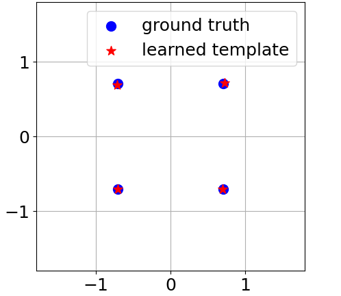
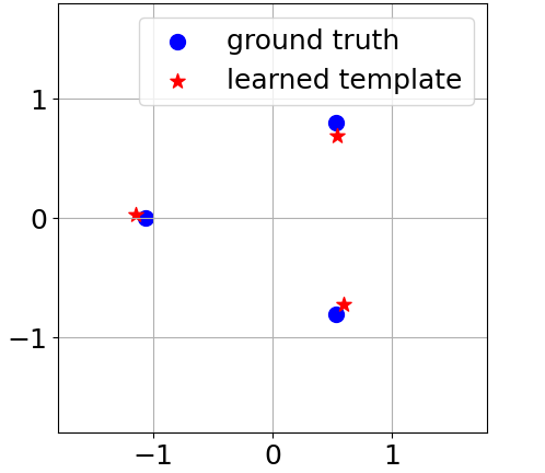
square, $\sigma=0.1$	triangle, $\sigma=0.25$

Figure 4: Visualization of GT templates and Procrustes transformed learned templates, after training with scenes of different noise levels.

8.2 Faces: experiments and results

Below we provide details of the data generator and inference methods for the faces data in sec. 8.2.1, and give inference results in sec. 8.2.2.

8.2.1 Parts-based face model

We have developed a novel hierarchical parts-based model for face appearances. It is based on five parts, namely eyes, nose, mouth, hair and forehead, and jaw (see Fig. 1(b)). Each part has a specified mask, and we have cropped the hair region to exclude highly variable hairstyles. This decomposition is based on the "PhotoFit Me" work and data of Prof. Graham Pike, see https://www.open.edu/openlearn/PhotoFitMe. For each part we trained a probabilistic PCA (PPCA) model to reduce the dimensionality of the raw pixels; the dimensionality is chosen so as to explain 95% of the variance. This resulted in dimensionalities of 24, 11, 12, 16 and 28 for the eyes, nose, mouth, jaw and hair parts respectively. We then add a factor analysis (FA) model on top with latent variables ${\mathbf{y}}^{a}_{k}$ to model the correlations of the PPCA coefficients across parts. The dataset used (from PhotoFit Me) is balanced by gender (female/male) and by race (Black/Asian/Caucasian), hence the high-level factor analyser can model regularities across the parts, e.g. wrt skin tone. ${\mathbf{x}}^{a}_{n}$ is predicted from ${\mathbf{y}}^{a}_{k}$ as $F^{a}_{kn}{\mathbf{y}}^{a}_{k}+\bm{m}^{a}_{kn}$ as in (5). ${\mathbf{y}}^{g}_{k}$ would have an effect on the part appearance, e.g. by scaling and rotation, but this can be removed by running the PPCA part detectors on copies of the input image that have been rescaled and rotated.

The “PhotoFit Me” project utilizes 7 different part-images for each gender/race group, for each of the five part types. As a result, we generated $7^{5}$ synthetic faces for each group, by combining these face-parts, which led to a total of $100,842$ faces. All faces were centered on a $224\times 224$ pixel canvas. For each synthetic face we created an appearance vector ${\mathbf{x}}^{a}_{n}$, which consisted of the stacked vectors from the 5 different principal component subspaces. Finally, we created a balanced subset from the generated faces ($18,000$ images), which we used to train a FA model. We tuned the latent dimension of this model by training it multiple times with a different number of factors, and finally chose 12 factors, where a knee in the reconstruction loss on the face data was observed on a validation set.

To evaluate our inference algorithm we generated $224\times 224$ pixel scenes of faces. These consisted of 2, 3, 4 or 5 randomly selected faces from a balanced test-set of $7,614$ synthetic faces, which were transformed with random similarity transformations. The face-objects were randomly scaled down by a minimum of 50% and were also randomly translated and rotated, with the constraint that all the faces fit the scene and did not overlap each other. An example of such a scene is shown in Fig. 1(c), and further examples are shown in Figure 5. For each scene it is easy to determine the correct number of faces, as the number of faces present is equal to the count of each of the parts detected. Afterwards, these two constraints were dropped to test the ability of our model to perform inference with occluded parts, see Figure 5(e) for an example. These occluded scenes were comprised of 3 faces. In our experiments we assume that the face parts are detected accurately, i.e. as generated.

In the case of facial parts—and parts with both geometric and appearance features in general—it only makes sense to assign the observed parts ${\mathbf{x}}_{m}$ to template parts ${\mathbf{x}}_{kn}$ of the same type (e.g. an observed “nose” part should be assigned only to a template “nose” part). We assume that this information is known, since the size of the appearance vector of each part-type is unique. Thus it no longer makes sense to initialize the assignment matrix uniformly for all entries, but rather only for the entries that correspond to templates of the observed part’s type. Consequently, (14) is only utilized for $m,n$ pairs of the same type. Similarly to the constellation experiments, we initialized the assignment matrix 5 times and selected the solution with the largest ELBO.

In the experiments we evaluated the part assignment accuracy of the algorithms. In a given scene, the assignment is considered correct if all the observed parts have been correctly assigned to their corresponding template parts with the highest probability. In order to evaluate the prediction of the appearance features, we measured the root mean square error (RMSE) between the input and generated scenes.

8.2.2 Face Experiments

Ground Truth	VI	RANSAC
(a)
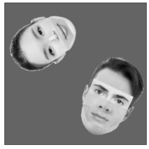
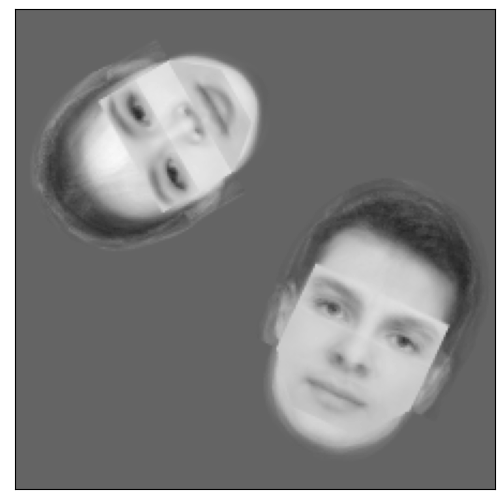
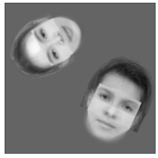
(b)
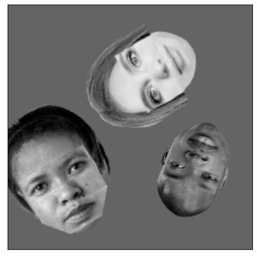
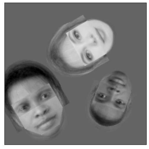
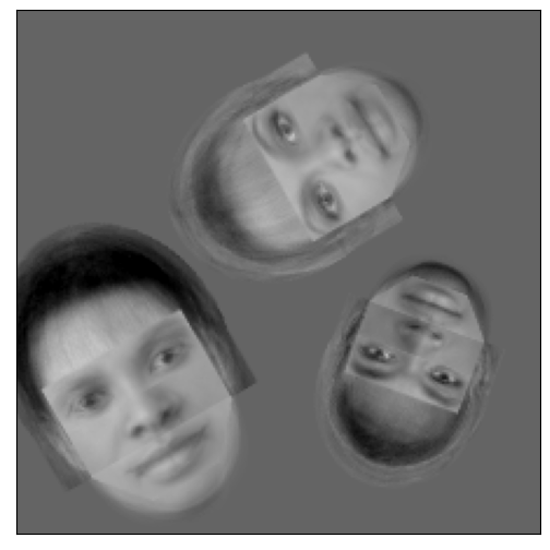
(c)
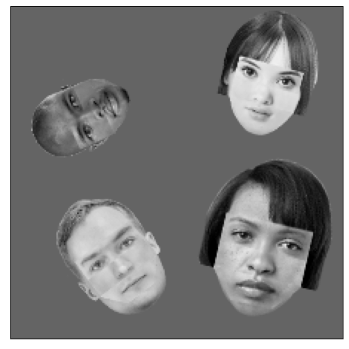
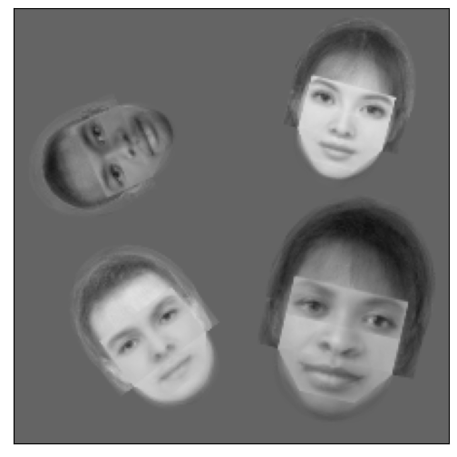
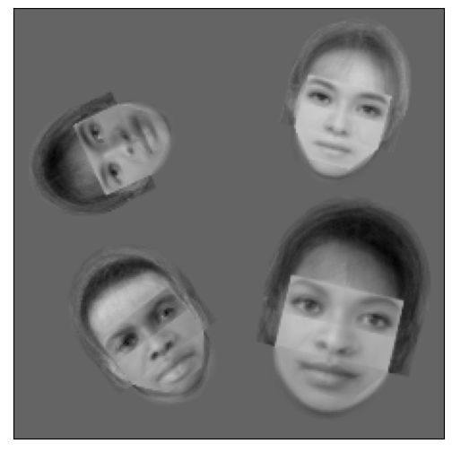
(d)
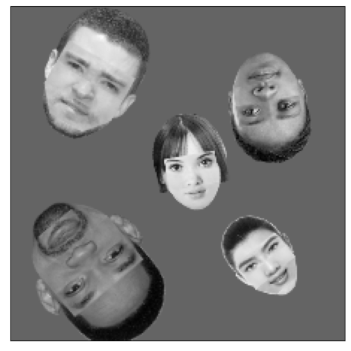
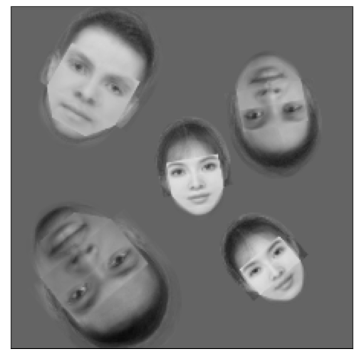
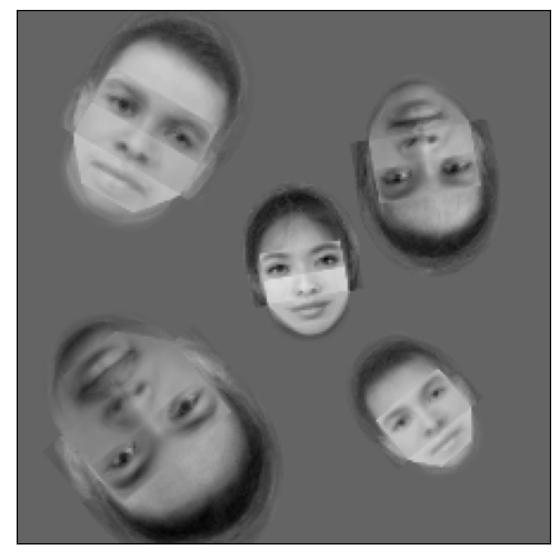
(e)

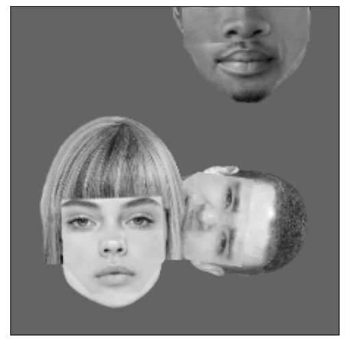
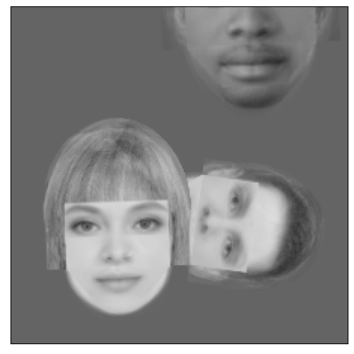
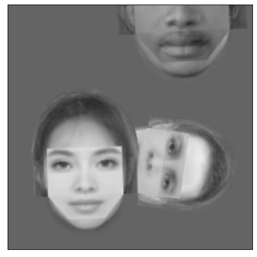
Figure 5: Reconstruction examples with our Variational Inference (VI) algorithm and the RANSAC-type algorithm: (a) scene with 2 faces, (b) scene with 3 faces, (c) scene with 4 faces (d) scene with 5 faces and (e) 3 faces with partially occluded faces. All faces have been randomly selected and transformed.

Firstly, the VI algorithm was evaluated on scenes of multiple, randomly selected and transformed faces. For scenes with 2, 3, 4 and 5 faces, the assignment accuracy was 100%, 100%, 99.2% and 93.7% respectively (based on 250 scenes per experiment). RANSAC gave 100% accurate assignments in all four cases. This is to be expected, since from each part the pose of the whole can be predicted accurately. However, RANSAC’s ability to infer the appearance of the faces proved to be limited. More specifically, in 250 instances uniformly distributed across scenes of 2, 3, 4 and 5 faces, the VI algorithm had RMSE of $0.036\pm 0.004$, while RANSAC scored $0.052\pm 0.006$, with consistently higher error on all scenes. This is illustrated in the examples of Figure 5, where it is clear that RANSAC is less accurate in capturing key facial characteristics. If inference for ${\mathbf{y}}^{a}_{k}$ is run as a post-processing step for RANSAC using all detected parts in an object, this difference disappears.

The supplementary material contains a movie showing the fitting of the models to the data. It is not possible for us to make a fair comparison with the SCAE algorithm on the faces data, as the PCAE model used is not rich enough to model PCA subspaces.

Secondly, we evaluated the ability of our algorithm to perform inference in scenes where some parts have been occluded, either by overlapping with other faces or by extending outside of the scene. In 250 scenes with 3 partially occluded faces, both the VI and RANSAC algorithms were fully successful in assigning the observed parts to the corresponding template accurately; see Figure 5(e) for an example.

9 Discussion

In our experiments RANSAC was shown to often be an effective alternative to variational inference (VI). This is particularly the case when the basis in RANSAC is highly informative about the object. For the constellations experiments this was the case, even when the datapoints were corrupted by noise. However, as we saw in sec. 8.2.2 for the faces data, an individual part was less informative about the appearance than the geometry, and so led to worse reconstructions unless a post-processing step using all of the detected parts was used. Also, RANSAC’s sampling-based inference may be less amenable to neural-network style parallel implementations than VI.

Above we have described a generative capsules model. The key features of this approach are:

• The model is interpretable, and thus admits the use of prior knowledge, e.g. if we already know some things about an object. The formulation is also composable in that models for individual objects can be learned separately, then combined together at inference time.

• The variational inference algorithm is obtained directly from a generative model for the observations $X$. In contrast other leading formulations set up an objective to produce clusters in ${\mathbf{y}}$-space.

• The interpretable structure of the GCM allows other inference methods to be used, as demonstrated by our use of RANSAC.

• The GCM conforms to the view, as promoted in Kosiorek et al., (2019), that the input is regarded as a set of parts. This formulation ensures that if the parts can be detected equivariantly, then the inferences for the objects will also be equivariant. This was demonstrated in the constellations and faces experiments.

As noted above, for the GCM to be equivariant to large transformations of the input, the parts need to to be detected equivariantly. Some capsules papers have used the affNIST dataset, but this only used small rotations of up to $\pm 20^{\circ}$. Hinton et al., (2018, sec. 5.1) did investigate the use of very different viewpoints on the smallNORB dataset; while their capsules results in Table 2 did outperform a competitor CNN, it is noticeable that there is still a performance gap between novel and familiar viewpoints. We have demonstrated (see Fig. 2) that the PCAE decomposition is not equivariant to large rotations, and similar observations have been made by Smith et al., (2021) for their model. Thus we believe that further work on the equivariant extraction of parts is necessary in order to achieve equivariant object recognition.

Acknowledgements

We thank the anonymous referees for their helpful comments. This work was supported in part by The Alan Turing Institute under EPSRC grant EP/N510129/1. For the purpose of open access, the authors have applied a Creative Commons Attribution (CC BY) licence to any Author Accepted Manuscript version arising from this submission.

Appendix A Details for Variational Inference

The evidence lower bound (ELBO) $L(q)={\mathbb{E}}_{q}[\log p(X,Y,Z)-\log q(Y,Z)]$ for this model is decomposed in three terms:

$$L(q) ={\mathbb{E}}_{q}[\log{p(X|Y,Z)}]-KL(q(Y)||p(Y))-KL(q(Z)||p(Z)),$$ (22)

where $KL(q||p)$ is the Kullback-Leibler divergence between distributions $q$ and $p$. The first term indicates how well the generative model $p(X|Y,Z)$ fits the observations under our variational model $q(Y,Z)$:

$${\mathbb{E}}_{q}[\log{p(X|Y,Z)}]=-\sum_{m=1}^{M}\sum_{k=1}^{K}\sum_{n=1}^{N_{k}}r_{mnk}\Big{[}\frac{d_{kn}}{2}\log{2\pi}+\frac{1}{2}\log{|\beta^{-1}D_{kn}|}+\Big{.}$$

$$\frac{\beta}{2}({\mathbf{x}}_{m}-F_{kn}{\bm{\mu}}_{k}-\bm{m}_{kn})^{T}D_{kn}^{-1}({\mathbf{x}}_{m}-F_{kn}{\bm{\mu}}_{k}-\bm{m}_{kn})+\Big{.}\frac{\beta}{2}\text{trace}(F_{kn}^{T}D_{kn}^{-1}F_{kn}\Lambda_{k}^{-1})\Big{]}.$$ (23)

The Kullback-Leibler divergence between the two Gaussian distributions $q(Y)$ and $p(Y)$ in our model has the following expression:

$$KL(q(Y)||p(Y))=\\ \frac{1}{2}\sum_{k=1}^{K}\left(\text{trace}(D^{-1}_{0}\Lambda^{-1}_{k})-d_{k}+({\bm{\mu}}_{k}-{\bm{\mu}}_{0})^{T}D_{0}^{-1}({\bm{\mu}}_{k}-{\bm{\mu}}_{0})+\log{|D_{0}|}+\log{|\Lambda_{k}|}\right),$$ (24)

where $d_{k}$ is the dimensionality of ${\mathbf{y}}_{k}$.

The expression for $KL(q(Z)||p(Z))$ is given by

$$KL(q(Z)||p(Z)) =\sum_{m=1}^{N}\sum_{k=1}^{K}\sum_{n=1}^{N_{k}}r_{mnk}\log{\frac{r_{mnk}}{a_{mnk}}}.$$ (25)

Appendix B Learning for the Constellations Model

We specialize the ELBO given in Appendix A for one constellation, taking $K=1$ (and hence dropping the index $k$). As there are no appearance features, we drop the $g$ superscript on $F_{n}$ and ${\mathbf{y}}$. Also the mean $\bm{m}_{kn}$ is only needed for the appearance features and thus can be omitted. $D_{n}$ is specialized to $\lambda^{-1}I_{2}$, we set $\beta=1$ in this appendix and allow $\lambda$ to vary, and we assume $p({\mathbf{y}})\sim N({\bm{0}},\Lambda_{0}^{-1})$. Hence by specializing eq. 23 we obtain

$${\mathbb{E}}_{q}[\log{p(X|Y,Z)}]=\\ -\sum_{m=1}^{M}\sum_{n=1}^{N}r_{mn}\Big{[}\log\frac{2\pi}{\lambda}+\frac{\lambda}{2}({\mathbf{x}}_{m}-F_{n}{\bm{\mu}})^{T}({\mathbf{x}}_{m}-F_{n}{\bm{\mu}})+\frac{\lambda}{2}\text{trace}(F_{n}^{T}F_{n}\Lambda^{-1})\Big{]},$$ (26)

where $q({\mathbf{y}})\sim N({\bm{\mu}},\Lambda^{-1})$, with $\Lambda$ and ${\bm{\mu}}$ specialized from eqs. 19 and 20 as

$$\Lambda=\Lambda_{0}+\lambda\sum_{m=1}^{M}\sum_{n=1}^{N}r_{mn}F_{n}^{T}F_{n},\qquad{\bm{\mu}}=\lambda\;\Lambda^{-1}(\sum_{m=1}^{M}\sum_{n=1}^{N}r_{mn}F_{n}^{T}{\mathbf{x}}_{m}).$$ (27)

Our goal in learning is to adapt the template parameters $\{F_{n}\}$ so as to increase the variational log likelihood (ELBO) $L(q)$. In the M-step of variational EM, the distributions $q({\mathbf{y}})$ and $q(Z)$ (parameterized by ${\bm{\mu}}$, $\Lambda$ and $R$) are held fixed, and the ELBO is optimized wrt $\{F_{n}\}$. Note that the terms $KL(q(Y)||p(Y))$ and $KL(q(Z)||p(Z))$ do not depend explicitly on $\{F_{n}\}$, and hence any derivative of these KL terms wrt $F_{n}$ will be zero. Thus these terms can be omitted when optimizing the ELBO wrt $\{F_{n}\}$.

The trace term in eq. 26 can be simplified using $\sum_{m}r_{mn}=1$, to give

$$\sum_{m=1}^{M}\sum_{n=1}^{N}r_{mn}\text{trace}(F_{n}^{T}F_{n}\Lambda^{-1})=\text{trace}((\sum_{n=1}^{N}F_{n}^{T}F_{n})\Lambda^{-1}).$$ (28)

It turns out that it is more convenient to write $F_{n}{\bm{\mu}}$ in terms of ${\mathbf{p}}_{n}=(p_{nx},p_{ny})^{T}$ and the mean transformation parameters ${\bm{\mu}}=(\hat{t}_{x},\hat{t}_{y},\hat{s}_{c},\hat{s}_{s})^{T}$, where $\hat{s}_{c}$ is the posterior mean of $s\cos\theta$, and $\hat{s}_{s}$ is the same for $s\sin\theta$. Hence we have that

$$F_{n}{\bm{\mu}} =\begin{pmatrix}\hat{{\mathbf{t}}}_{x}\\ \hat{t}_{y}\end{pmatrix}+\begin{pmatrix}\hat{s}_{c}&\hat{s}_{s}\\ -\hat{s}_{s}&\hat{s}_{c}\end{pmatrix}\begin{pmatrix}p_{nx}\\ p_{ny}\end{pmatrix}{\stackrel{{\scriptstyle def}}{{=}}}\;\hat{{\mathbf{t}}}+\hat{T}{\mathbf{p}}_{n}.$$ (29)

Hence ${\mathbf{x}}_{m}-F_{n}{\bm{\mu}}={\mathbf{x}}_{m}-\hat{{\mathbf{t}}}-\hat{T}{\mathbf{p}}_{n}=\tilde{{\mathbf{x}}}_{m}-\hat{T}{\mathbf{p}}_{n}$, where $\tilde{{\mathbf{x}}}_{m}={\mathbf{x}}_{m}-\hat{{\mathbf{t}}}$, and the quadratic form $({\mathbf{x}}_{m}-F_{n}{\bm{\mu}})^{T}({\mathbf{x}}_{m}-F_{n}{\bm{\mu}})$ can be rewritten as $(\tilde{{\mathbf{x}}}_{m}-\hat{T}{\mathbf{p}}_{n})^{T}(\tilde{{\mathbf{x}}}_{m}-\hat{T}{\mathbf{p}}_{n})$.

We can now rewrite the term $Q=\sum_{m}\sum_{n}r_{mn}({\mathbf{x}}_{m}-F_{n}{\bm{\mu}})^{T}({\mathbf{x}}_{m}-F_{n}{\bm{\mu}})$ in eq. 26 as

$$Q =\sum_{m}\sum_{n}r_{mn}(\tilde{{\mathbf{x}}}_{m}-\hat{T}{\mathbf{p}}_{n})^{T}(\tilde{{\mathbf{x}}}_{m}-\hat{T}{\mathbf{p}}_{n})$$ (30)

$$=\sum_{m}\sum_{n}r_{mn}\left({\mathbf{p}}_{n}^{T}\hat{T}^{T}\hat{T}{\mathbf{p}}_{n}-{\mathbf{p}}_{n}^{T}\hat{T}^{T}\tilde{{\mathbf{x}}}_{m}-\tilde{{\mathbf{x}}}_{m}^{T}\hat{T}p_{n}+\tilde{{\mathbf{x}}}_{m}^{T}\tilde{{\mathbf{x}}}_{m}\right).$$ (31)

Using $\sum_{m}r_{mn}=1$ and defining $\tilde{{\mathbf{x}}}_{n}^{r}=\sum_{m}r_{mn}\tilde{{\mathbf{x}}}_{m}$, we obtain

$$Q=\sum_{n}{\mathbf{p}}_{n}^{T}\hat{T}^{T}\hat{T}{\mathbf{p}}_{n}-{\mathbf{p}}_{n}^{T}\hat{T}^{T}\tilde{{\mathbf{x}}}^{r}_{n}-(\tilde{{\mathbf{x}}}^{r}_{n})^{T}\hat{T}{\mathbf{p}}_{n}+(\sum_{m,n}r_{mn}\tilde{{\mathbf{x}}}_{m}^{T}\tilde{{\mathbf{x}}}_{m}).$$ (32)

This can be further simplified by noting that $\hat{T}^{T}\hat{T}=\hat{s}^{2}I_{2}$, where $\hat{s}^{2}=\hat{s}^{2}_{c}+\hat{s}^{2}_{s}$.

The above derivation is all for one example $X$. Now summing $Q$ over all training examples $\{X_{i}\}$ we obtain

$$Q^{tot}=\sum_{i}Q_{i}=\sum_{i}\sum_{n}\left(\hat{s}^{2}_{i}{\mathbf{p}}_{n}^{T}{\mathbf{p}}_{n}-{\mathbf{p}}_{n}^{T}\hat{T}^{T}\tilde{{\mathbf{x}}}^{r}_{ni}-(\tilde{{\mathbf{x}}}^{r}_{ni})^{T}\hat{T}{\mathbf{p}}_{n}+\sum_{m}r_{mn}\tilde{{\mathbf{x}}}_{mi}^{T}\tilde{{\mathbf{x}}}_{mi}\right),$$ (33)

where $\tilde{{\mathbf{x}}}^{r}_{ni}$ denotes $\tilde{{\mathbf{x}}}^{r}_{n}$ in the $i$th example, and similarly for $\tilde{{\mathbf{x}}}_{mi}$.

Now consider the trace term $S_{i}=\text{trace}((\sum_{n=1}^{N}F_{n}^{T}F_{n})\Lambda_{i}^{-1})$, where $\Lambda_{i}$ is the precision matrix for ${\mathbf{y}}$ on the $i$th example. We have that

$$F_{n}^{T}F_{n}=\begin{pmatrix}1&0\\ 0&1\\ p_{nx}&p_{ny}\\ p_{ny}&-p_{nx}\end{pmatrix}\begin{pmatrix}1&0&p_{nx}&p_{ny}\\ 0&1&p_{ny}&-p_{nx}\end{pmatrix}=\begin{pmatrix}1&0&p_{nx}&p_{ny}\\ 0&1&p_{ny}&-p_{nx}\\ p_{nx}&p_{ny}&p^{2}_{nx}+p^{2}_{ny}&0\\ p_{ny}&-p_{nx}&0&p^{2}_{nx}+p^{2}_{ny}\end{pmatrix}.$$ (34)

Assume that the template is centered so that $\sum_{n}p_{nx}=\sum_{n}p_{ny}=0$, and scaled so that $\sum_{n}p^{2}_{nx}+p^{2}_{ny}=N$. Hence we have that $\sum_{n}F_{n}^{T}F_{n}=NI_{4}$. From eq. 27 and taking $\Lambda_{0}=\alpha I_{4}$ we have

$$\Lambda=\Lambda_{0}+\sum_{m}\sum_{n}r_{mn}F_{n}^{T}F_{n}=(\alpha+\lambda N)I_{4}.$$ (35)

Hence

$$\text{trace}((\sum_{n=1}^{N}F_{n}^{T}F_{n})\Lambda^{-1})=N\text{trace}(\Lambda^{-1})=\frac{4N}{\alpha+\lambda N}.$$ (36)

Crucially, this term is independent of $\{{\mathbf{p}}_{n}\}$, as long as the template is centered and scaled correctly. Hence this term can be ignored when optimizing the ${\mathbf{p}}_{n}$s.

Thus optimizing the ELBO wrt ${\mathbf{p}}_{n}$ comes down to optimizing $Q^{tot}$ wrt ${\mathbf{p}}_{n}$. Differentiating eq. 33 wrt ${\mathbf{p}}_{n}$ and setting it equal to zero we obtain

$$\frac{\partial{Q^{tot}}}{\partial{{\mathbf{p}}_{n}}}=\sum_{i}\left(2\hat{s}^{2}_{i}{\mathbf{p}}_{n}-2\hat{T}_{i}^{T}\tilde{{\mathbf{x}}}^{r}_{ni}\right)=0,$$ (37)

which gives the update formula

$${\mathbf{p}}_{n}=\frac{1}{\sum_{i}\hat{s}_{i}^{2}}\sum_{i}\hat{T}^{T}_{i}\tilde{{\mathbf{x}}}^{r}_{ni}.$$ (38)

It can also be shown that $\hat{T}^{T}=\hat{s}^{2}\hat{T}^{-1}$, yielding the update equation

$${\mathbf{p}}_{n}=\frac{\sum_{i}\hat{s}_{i}^{2}\hat{T}^{-1}_{i}\tilde{{\mathbf{x}}}^{r}_{ni}}{\sum_{i}\hat{s}_{i}^{2}}.$$ (39)

This is quite intuitive—we first remove the effect of the translation $\hat{{\mathbf{t}}}$ by computing $\tilde{{\mathbf{x}}}_{m}$, then take into account the weighted assignments $r_{mn}$ to give $\tilde{{\mathbf{x}}}^{r}_{ni}$, and then apply $\hat{T}^{-1}_{i}$ to remove the effect of the scaling and rotation. The summations are weighted by $\hat{s}_{i}^{2}$, which has the effect giving higher weight to examples with larger scale, where the relative effect of the noise $N(0,\lambda^{-1})$ is smaller.

One can also re-estimate $\lambda$ using the variational EM algorithm. Differentiating eq. 26 wrt $\lambda$ we obtain

$$\frac{1}{\lambda}=\frac{1}{2NS}\sum_{i=1}^{S}\sum_{m,n}r^{i}_{mn}({\mathbf{x}}_{mi}-F_{n}{\bm{\mu}}_{i})^{T}({\mathbf{x}}_{mi}-F_{n}{\bm{\mu}}_{i}),$$ (40)

where $S$ denotes the number of examples. As $\lambda^{-1}$ is a variance, this equation makes sense in terms of an average of squared residuals. In the derivation of eq. 40 the dependence of the trace term $4N\lambda/(\alpha+N\lambda)$ on $\lambda$ has been omitted, as for $N\lambda\gg\alpha$ this dependence is negligible.

Appendix C Evaluation metrics for the constellations data

In a given scene $X$ there are $M$ points, but we know that there are $N\geq M$ possible points that can be produced from all of the templates. Assume that $K^{\prime}\leq K$ templates are active in this scene. Then the points in the scene are labelled with indices $1,\ldots,K^{\prime}$, and we assign the missing points index $0$. Denote the ground truth partition as $V=\{V_{0},V_{1},\ldots V_{K^{\prime}}\}$. An alternative partition output by one of the algorithms is denoted by $\hat{V}=\{\hat{V}_{0},\hat{V}_{1},\ldots\hat{V}_{\hat{K}^{\prime}}\}$. The predicted partition $\hat{V}$ may instantiate objects or points that were in fact missing, thus it is important to handle the missing data properly.

In Information Theory, the variation of information (VI) (Meilă,, 2003) is a measure of the distance between two partitions of elements (or clusterings). For a given set of elements, the variation of information between two partitions $V$ and $\hat{V}$, where $N=\sum_{i}|V_{i}|=\sum_{j}|\hat{V}_{j}|$ is defined as:

$$VI(V,\hat{V})=-\sum_{i,j}r_{ij}\left[\log{\frac{r_{ij}}{p_{i}}}+\log{\frac{r_{ij}}{q_{j}}}\right]$$ (41)

where $r_{ij}=\frac{|V_{i}\cap\hat{V}_{j}|}{N}$, $p_{i}=\frac{|V_{i}|}{N}$ and $q_{j}=\frac{|\hat{V}_{j}|}{N}$. In our experiments we report the average variation of information of the scenes in the dataset.

The Rand index (Rand,, 1971) is another measure of similarity between two data clusterings. This metric takes pairs of elements and evaluates whether they do or do not belong to the same subsets in the partitions $V$ and $\hat{V}$

$$RI=\frac{TP+TN}{TP+TN+FP+FN},$$ (42)

where TP are the true positives, TN the true negatives, FP the false positives and FN the false negatives. The Rand index takes on values between 0 and 1. We use instead the adjusted Rand index (ARI) (Hubert and Arabie,, 1985), the corrected-for-chance version of the Rand index. It uses the expected similarity of all pair-wise comparisons between clusterings specified by a random model as a baseline to correct for assignments produced by chance. Unlike the Rand index, the adjusted Rand index can return negative values if the index is less than the expected value. In our experiments, we compute the average adjusted Rand index of the scenes in our dataset.

The segmentation accuracy (SA) is based on obtaining the maximum bipartite matching between $V$ and $\hat{V}$, and was used by Kosiorek et al., (2019) to evaluate the performance of CCAE. For each set $V_{i}$ in $V$ and set $\hat{V}_{j}$ in $\hat{V}$, there is an edge $w_{ij}$ with the weight being the number of common elements in both sets. Let $W(V,\hat{V})$ be the overall weight of the maximum matching between $V$ and $\hat{V}$. Then we define the average segmentation accuracy as:

$$SA=\sum_{i=1}^{I}\frac{W(V_{i},\hat{V}_{i})}{W(V_{i},V_{i})}=\frac{1}{N}\sum_{i=1}^{I}W(V_{i},\hat{V}_{i}),$$ (43)

where $I$ is the number of scenes. Notice that $W(V_{i},V_{i})$ represents a perfect assignment of the ground truth, both the observed and missing subsets, and thus $W(V_{i},V_{i})=N$.

There are some differences on how we compute the SA metric compared to Kosiorek et al., (2019). First, they do not consider the missing points as part of their ground truth, but as we argued above this is necessary. They evaluate the segmentation accuracy in terms of the observed points in the ground truth, disregarding possible points that were missing in the ground truth but predicted as observed in $\hat{V}$. Second, they average the segmentation accuracy across scenes as

$$SA=\frac{\sum_{i=1}^{I}W(V_{i},\hat{V}_{i})}{\sum_{i=1}^{I}W(V_{i},V_{i})}.$$ (44)

For them, $W(V_{i},V_{i})=M_{i}$, where $M_{i}$ is the number of points present in a scene. In our case, both averaging formulae are equivalent since our $W(V_{i},V_{i})$ is the same across scenes.

Appendix D Failures of rotation equivariance for SCAE

We trained the SCAE model with digit “4” images from the training set of the MNIST dataset, after they had been uniformly rotated by up to $360^{\circ}$ and uniformly translated by up to 6 pixels on the x and y axes. Since we used a single class in the dataset we modified the SCAE architecture to use only a single object capsule.

We repeated the training of SCAE multiple times for 8K epochs, and collected distinct sets of learned $11\times 11$ parts that the digit “4” can be decomposed into. Two example part-sets are shown in Fig. 2. We then evaluated PCAE’s ability to detect these parts in MNIST digit “4” images that had been rotated by multiples of $45^{\circ}$. Our results indicate that the PCAE model is not equivariant to rotations. This is apparent from Fig. 2, where the learned parts are inconsistently assigned to the regions of the digit-object, depending on the angle of rotation. We hypothesize that this phenomenon stems from the fact that PCAE seems to generate parts that are either characterized by an intrinsic symmetry, and thus their pose is ambiguous, as in the line features of part-set-a in Fig. 2); or pairs of parts that are transformed versions of themselves, and thus can be used interchangeably (e.g. the first and third templates of part-set-b in Fig. 2). This leads to identifiability issues, where the object can be decomposed into its parts in numerous ways.

Appendix E Examples of Noisy Cases

Figure 6 shows several examples of objects generated from noisy templates with a corruption level of $\sigma=0.25$. GCM-DS and RANSAC do not allow for deformable objects to try to fit the points exactly, contrary to CCAE. Both methods try to find the closest reconstruction of the noisy points in the image by selecting the geometrical shapes that are a best fit to those points. Nonetheless, both methods can determine that which parts belong together to form a given object, even when the matching is not perfect.

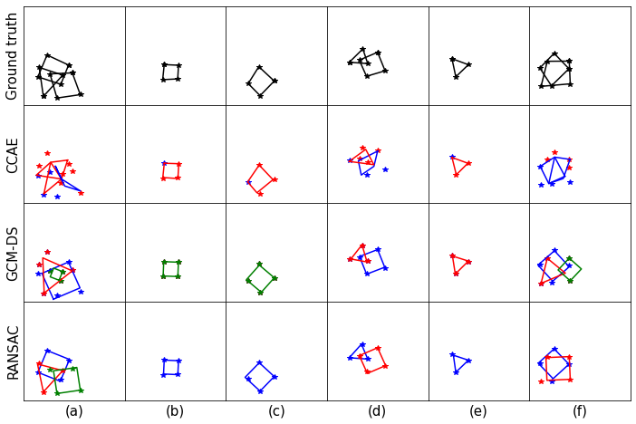
Figure 6: Reconstruction examples from CCAE, GCM-DS and RANSAC with Gaussian noise $\sigma=0.25$.

References

- Basri, (1996) Basri, R. (1996). Paraperspective Affine. International Journal of Computer Vision, 19:169–179.
- Bengio et al., (2009) Bengio, Y., Louradour, J., Collobert, R., and Weston, J. (2009). Curriculum Learning. In Proc. 26th International Conference on Machine Learning.
- Biederman, (1987) Biederman, I. (1987). Recognition-by-Components: A Theory of Human Image Understanding. Psychological Review, 94:115–147.
- Bishop, (2006) Bishop, C. M. (2006). Pattern Recognition and Machine Learning. Springer.