A new analysis of the three–body problem

Abstract

In the recent papers [18], [5], respectively, the existence of motions where the perihelions afford periodic oscillations about certain equilibria and the onset of a topological horseshoe have been proved. Such results have been obtained using, as neighbouring integrable system, the so–called two–centre (or Euler) problem and a suitable canonical setting proposed in [16], [17]. Here we review such results.

1 Overview

In the recent papers [5], [18] the existence, in the three–body problem (3BP), of motions which by no means can be regarded as “extending” in some way Keplerian motions has been proved. Indeed, the motions found in those papers can be better understood as continuations of the motions of the so–called two–centre problem (or Euler problem; 2CP from now on).
The motivation that pushed such researches was a new analysis of 2CP carried out in [17], combined with a remarkable property – which we called renormalizable integrability – pointed out in [16]. It relates the “simply averaged Newtonian potential” (see the precise definition below) and the function, which in this paper we shall refer to as Euler integral, that makes the 2CP integrable. Roughly, such property states that the averaged Newtonian potential and the Euler integral have the same motions, as they are one a function of the other. As, on the other hand, the motions of the Euler integral are, at least qualitatively, explicit, and the averaged Newtonian potential is a prominent part of the 3BP Hamiltonian, the papers [5], [18] gave partial answers to the natural question whether the motions of the Euler integral can be traced in 3BP. Let us introduce some mathematical tools in order to make our statements more precise.

In terms of Jacobi coordinates [10] the three–body problem Hamiltonian with masses $1$, ${\mu}$, ${\kappa}$ is the translation–free function

$${{\rm H}_{\rm J}} = \frac{\|\mathbf{y}\|^{2}}{2}\left(1+\frac{1}{{\mu}}\right)+\frac{\|\mathbf{y}^{\prime}\|^{2}}{2}\left(\frac{1}{1+{\mu}}+\frac{1}{{\kappa}}\right)-\frac{{\mu}}{\|\mathbf{x}\|}-\frac{{\mu}{\kappa}}{\|\mathbf{x}^{\prime}-\frac{1}{1+{\mu}}\mathbf{x}\|}$$

$$-\frac{{\kappa}}{\|\mathbf{x}^{\prime}+\frac{{\mu}}{1+{\mu}}\mathbf{x}\|}\,.$$

Here, $({\mathbf{y}}^{\prime},{\mathbf{y}},{\mathbf{x}}^{\prime},{\mathbf{x}})\in({{R}}^{3})^{4}$ (or $({{R}}^{2})^{4}$, in the planar case), $\|\cdot\|$ denotes Euclidean norm and the gravity constant has been taken equal to one, by a proper choice of the units system. We rescale impulses and positions

$${\mathbf{y}\to\frac{{\mu}}{1+{\mu}}\mathbf{y}\,,\quad\mathbf{x}\to{(1+{\mu})}{\mathbf{x}}\,,\quad\mathbf{y}^{\prime}\to{\mu}{\beta}{\mathbf{y}^{\prime}}\,,\quad\mathbf{x}^{\prime}\to{\beta}^{-1}\mathbf{x}^{\prime}},$$ (1)

multiply the Hamiltonian by $\frac{1+{\mu}}{{\mu}}$ (by a rescaling of time) and obtain

$${{\rm H}_{\rm J}=\frac{\|\mathbf{y}\|^{2}}{2}-\frac{1}{\|\mathbf{x}\|}+{\gamma}\left(\frac{\|\mathbf{y}^{\prime}\|^{2}}{2}-\frac{\overline{{\beta}}}{{\beta}+\overline{{\beta}}}\frac{1}{\|\mathbf{x}^{\prime}-{\beta}\mathbf{x}\|}-\frac{{\beta}}{{\beta}+\overline{{\beta}}}\frac{1}{\|\mathbf{x}^{\prime}+\overline{{\beta}}\mathbf{x}\|}\right)},$$ (2)

with

$${{\gamma}=\frac{{\kappa}^{3}(1+{\mu})^{4}}{{\mu}^{3}(1+{\mu}+{\kappa})}\,,\quad{\beta}=\frac{{\kappa}^{2}(1+{\mu})^{2}}{{\mu}^{2}(1+{\mu}+{\kappa})}\,,\quad\overline{{\beta}}={\mu}{\beta}}\,.$$ (3)

Likewise, one might consider the problem written in the so–called $1$–centric coordinates. In that case,

$${\rm H}_{0} = \frac{\|{\mathbf{y}}\|^{2}}{2}-\frac{1}{\|{\mathbf{x}}\|}+{\gamma}\left(\frac{\|{\mathbf{y}}^{\prime}\|^{2}}{2}-\frac{{\beta}}{{\beta}+\overline{{\beta}}}\frac{1}{\|{\mathbf{x}}^{\prime}\|}-\frac{\overline{{\beta}}}{{\beta}+\overline{{\beta}}}\frac{1}{\|{\mathbf{x}}^{\prime}-({\beta}+\overline{{\beta}}){\mathbf{x}}\|}\right)$$ (4)

$$+\overline{{\beta}}\,{{\mathbf{y}}^{\prime}\cdot{\mathbf{y}}},$$

with ${\gamma}$, ${\beta}$ and $\overline{{\beta}}$ analogous to (3), up to replace the factors $(1+{\mu}+{\kappa})$ with $(1+{\kappa})$. Note that we are not assuming ${\mu}$, ${\kappa}\ll 1$ (in fact, in our applications, we shall make different choices), which means that Jacobi or $1$–centric coordinates above are not necessarily centered at the most massive body. In order to simplify the analysis, we introduce a main assumption. Both the Hamiltonians ${\rm H}_{\rm J}$ and ${\rm H}_{0}$ in (2) and (4) include the Keplerian term

$${\rm J}_{0}:=\frac{\|\mathbf{y}\|^{2}}{2}-\frac{1}{\|\mathbf{x}\|}=-\frac{1}{2{\Lambda}^{2}}\,.$$ (5)

We assume that ${\rm J}_{0}$ is a “leading” term in such Hamiltonians. By averaging theory, this assumption allows us to replace (at the cost of a small error) ${\rm H}_{\rm J}$ and ${\rm H}_{0}$ with their respective $\ell$–averages

$$\overline{{\rm H}}_{i}=-\frac{1}{2{\Lambda}^{2}}+{\gamma}\mathaccent 866{{\rm H}}_{i}\,$$ (6)

with $i$=J,0, where $\ell$ is the mean anomaly associated to (5), and

$$\mathaccent 866{{\rm H}}_{\rm J} := \frac{\|{\mathbf{y}}^{\prime}\|^{2}}{2}-\frac{\overline{{\beta}}}{{\beta}+\overline{{\beta}}}{\rm U}_{{\beta}}-\frac{{\beta}}{{\beta}+\overline{{\beta}}}{\rm U}_{-\overline{{\beta}}}$$

$$\mathaccent 866{{\rm H}}_{0} := \frac{\|{\mathbf{y}}^{\prime}\|^{2}}{2}-\frac{\overline{{\beta}}}{{\beta}+\overline{{\beta}}}{\rm U}_{{\beta}+\overline{{\beta}}}-\frac{{\beta}}{{\beta}+\overline{{\beta}}}\frac{1}{\|{\mathbf{x}}^{\prime}\|}$$ (7)

with

$${\rm U}_{{\beta}}:=\frac{1}{2{\pi}}\int_{0}^{2{\pi}}\frac{d\ell}{\|{\mathbf{x}}^{\prime}-{\beta}{\mathbf{x}}(\ell)\|}.$$ (8)

In these formulae, the term $-\frac{1}{{2{\Lambda}^{2}}}$ will be referred to as “Keplerian term”, while terms of the form $-\frac{1}{\|{\mathbf{x}}^{\prime}-{\beta}{\mathbf{x}}\|}$ will be called “Newtonian potentials”. Therefore, ${\rm U}_{\beta}$ will be called “averaged Newtonian potential”. What we want to underline in that respect is that the averages (6) are “simple”, i.e., computed with respect to only one mean anomaly. Most often, in the literature double averages are considered; e.g. [14], [7], [15], [4],  [8], [11].

Whether and at which extent the Hamiltonians (6) are good approximations of (2), (4) is a demanding question, as, besides the mass parameters ${\mu}$, ${\kappa}$, also the region of phase space which is being considered plays a crucial rôle. We limit ourselves to some heuristics, focusing, in particular, on the case considered in [5]. Here the Hamiltonian (2) has been investigated, with ${\mu}=1\gg{\kappa}$, or, equivalently, ${\beta}=\overline{{\beta}}\gg 1$ (see (26) for the precise values). Physically, this corresponds to a couple of asteroids with equal mass interacting with a star, with ${\mathbf{x}}$ being the relative distance of the twin asteroids, and ${\mathbf{x}}^{\prime}$ the distance of the star from their center of mass. In that case, the region of phase space was chosen so that $\|{\mathbf{x}}^{\prime}\|>{\beta}\|{\mathbf{x}}\|$, so that the two denominators of the Newtonian potentials do not vanish. Expanding such Newtonian potentials in powers of $\frac{{\beta}a}{{\rm r}}$, where $a={\Lambda}^{2}$, ${\rm r}:=\|{\mathbf{x}}^{\prime}\|$, one sees that the lowest order terms depending on $\ell$ have size $\frac{\gamma{\beta}a}{{\rm r}^{2}}\sim\frac{{\kappa}^{3}a}{{\rm r}^{2}}$ (as ${\beta}\sim{\kappa}$, ${\gamma}\sim{\kappa}^{2}$). So, such terms are negligible compared to the size $\frac{1}{a}$ of the Keplerian term, provided that $\frac{{\kappa}^{3/2}a}{{\rm r}}\ll 1$.

We now turn to describe the main features of the Hamiltonians (6). Neglecting the Keplerian term, which is an inessential additive constant for $\overline{{\rm H}}_{i}$ and reabsorbing the constant ${\gamma}$ with a time change, we are led to look at the Hamiltonians $\mathaccent 866{{\rm H}}_{i}$ in (1), which, from now on, will be our object of study. Without loss of generality, we fix the constant action ${\Lambda}$ to $1$.

For definiteness and simplicity, we describe the setting in the case of the planar problem, in which case, after reducing the SO(2) symmetry, $\mathaccent 866{{\rm H}}_{i}$ have 2 degrees–of–freedom; all the generalisations to the spatial problem being described in Section 2. To describe the coordinates we used, we denote as $\mathbb{E}$ the Keplerian ellipse generated by Hamiltonian (5), for negative values of the energy. Assume $\mathbb{E}$ is not a circle. Remark that, as the mean anomaly $\ell$ is averaged out, we loose any information concerning the position of ${\mathbf{x}}$ on $\mathbb{E}$, so we shall only need two couples of coordinates for determining the shape of $\mathbb{E}$ and the vectors ${\mathbf{y}}^{\prime}$, ${\mathbf{x}}^{\prime}$. These are:

• the “Delaunay couple” $({\rm G},{\rm g})$, where ${\rm G}$ is the Euclidean length of ${\mathbf{x}}\times{\mathbf{y}}$ and ${\rm g}$ detects the perihelion. We remark that ${\rm g}$ is measured with respect to ${\mathbf{x}}^{\prime}$ (instead of with respect to a fixed direction), as the SO(2) reduction we use fixes a rotating frame which moves with ${\mathbf{x}}^{\prime}$ (compare the formulae in (81));

• the “radial–polar couple”$({\rm R},{\rm r})$, where ${\rm r}:=\|{\mathbf{x}}^{\prime}\|$ and ${\rm R}:=\frac{{\mathbf{y}}^{\prime}\cdot{\mathbf{x}}^{\prime}}{\|{\mathbf{x}}^{\prime}\|}$.

We now describe what we mean by renormalizable integrability [16]. Note first that, in terms of the coordinates above, the functions ${\rm U}_{\beta}({\rm r},{\rm G},{\rm g})$ in (8) depend on $({\rm r},{\rm G},{\rm g})$ and remark the homogeneity property

$${\rm U}_{\beta}({\rm r},{\rm G},{\rm g})={\beta}^{-1}{\rm U}({\beta}^{-1}{\rm r},{\rm G},{\rm g})\qquad{\rm where}\quad{\rm U}:={\rm U}_{1}\,.$$ (9)

By renormalizable integrability we mean that there exists a function ${\rm F}$ of two arguments such that the function ${\rm U}$ in (9) verifies

$${\rm U}({\rm r},{\rm G},{\rm g})={\rm F}({\rm E}_{0}({\rm r},{\rm G},{\rm g}),{\rm r})\,,$$ (10)

where

$${\rm E}_{0}({\rm r},{\rm G},{\rm g})={\rm G}^{2}+{\rm r}\sqrt{1-{\rm G}^{2}}\cos{\rm g}\,.$$ (11)

By (10), the level curves of ${\rm E}_{0}$ are also level curves of ${\rm U}$. On the other hand, the phase portrait of ${\rm E}_{0}$ in the plane $({\rm g},{\rm G})$ – i.e., the family of curves

$$\displaystyle{\rm E}_{0}({\rm r},{\rm G},{\rm g})={\rm G}^{2}+{\rm r}\sqrt{1-{\rm G}^{2}}\cos{\rm g}={\cal E},$$ (12)

in the plane $({\rm g},{\rm G})$ accordingly to the different values of ${\rm r}$ – is completely explicit [17]. For $0<{\rm r}<1$ or $1<{\rm r}<2$ it includes two minima $(\pm{\pi},0)$ on the ${\rm g}$–axis; two symmetric maxima on the ${\rm G}$–axis and one saddle point at $(0,0)$. When ${\rm r}>2$ the saddle point disappears and $(0,0)$ turns to be a maximum. The phase portrait includes two separatrices in the case $0<{\rm r}<2$; one separatrix in the case ${\rm r}>2$. These are the level set ${\cal S}_{0}({\rm r})$ through the saddle, corresponding to ${\cal E}={\rm r}$, for $0<{\rm r}<2$, and the level set ${\cal S}_{1}({\rm r})=\{{\cal E}=1\}$, for any ${\rm r}$. Rotational motions in between ${\cal S}_{0}({\rm r})$ and ${\cal S}_{1}({\rm r})$, do exist only for $0<{\rm r}<1$. The minima and the maxima are surrounded by librational motions and different motions (librations about different equilibria or rotations) are separated by ${\cal S}_{0}({\rm r})$ and ${\cal S}_{1}({\rm r})$. The reader is referred to Figure 1 for further qualitative details about the portion of the phase space corresponding to $[-\pi,\pi]\times[-1,1]$.

We call perihelium librations the librational motions about $(\pm{\pi},0)$ or $(0,0)$. Their physical meaning is that the perihelion of ${\mathbb{E}}$ affords oscillations while $\mathbb{E}$, highly eccentric anytime, periodically flattens to a segment in correspondence of the times when ${\rm G}$ vanishes. After the flattening time, the sense of rotation on $\mathbb{E}$ is reversed (as ${\rm G}$ changes its sign). We remark that (see the next section for a discussion) the potential ${\rm U}$ is well defined along the level sets of ${\rm E}$, with the exception of ${\cal S}_{0}({\rm r})$, where ${\rm U}$ is singular. In particular, ${\rm U}$ remains regular for all ${\rm r}>2$.

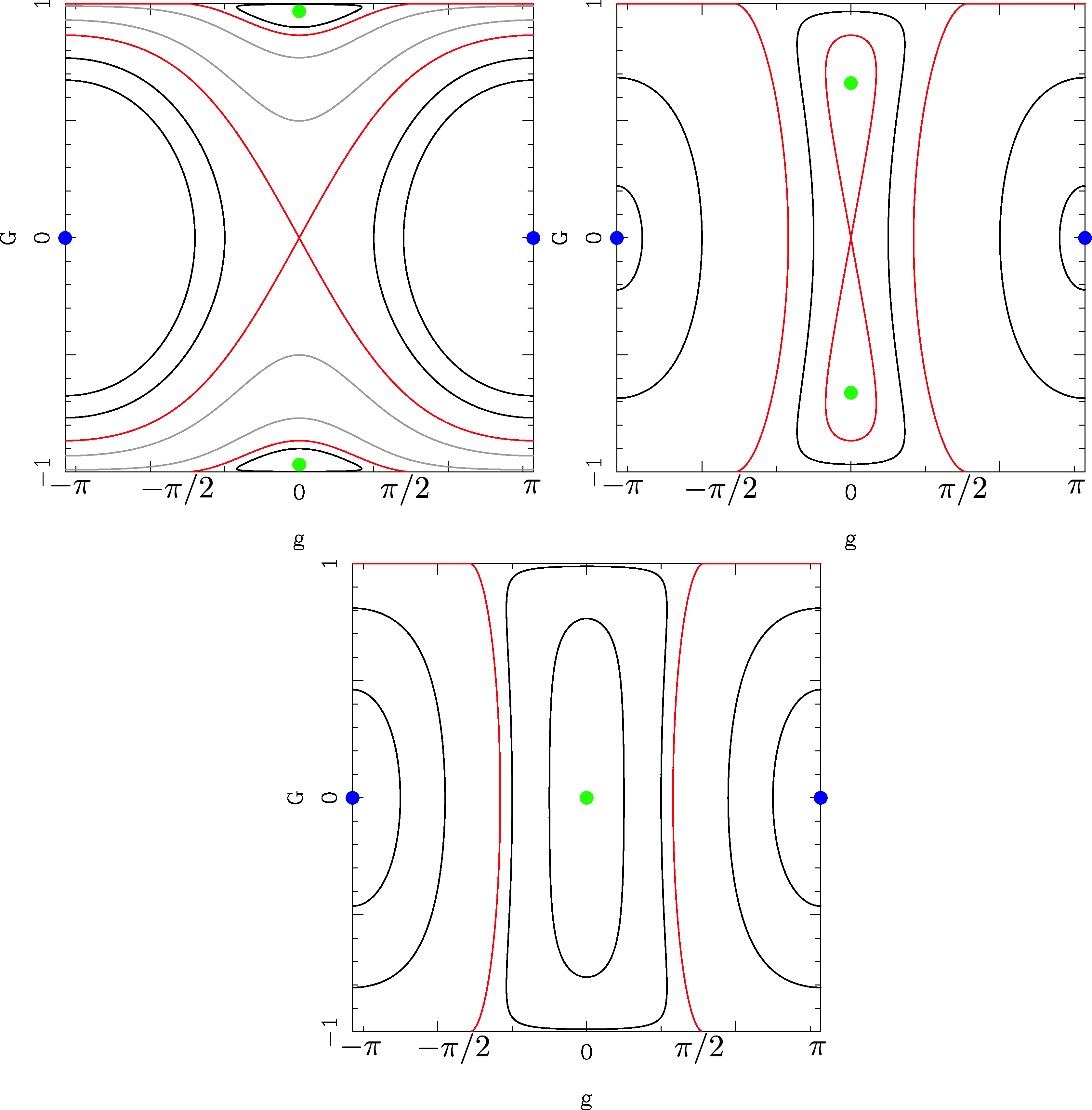
Figure 1: Phase portraits of $\textrm{E}_{0}$ given by (11) in the plane $(\textrm{g},\textrm{G})$ for $0<\textrm{r}<1$ (top left), $1<\textrm{r}<2$ (top right) and $\textrm{r}>2$ (bottom). The points corresponding to minima of $\textrm{E}_{0}$ are labeled in blue, maxima appear in green and separatrices correspond to red curves.

Let $0<{\beta}_{*}\leq{\beta}^{*}$ be defined via

$${\beta}_{*}:=\left\{\begin{array}[]{lll}\displaystyle\frac{{\beta}\overline{{\beta}}}{{\beta}+\overline{{\beta}}}&{\rm for}\ {\rm H}_{\rm J}\\ \\ \displaystyle\overline{{\beta}}&{\rm for}\ {\rm H}_{0}\end{array}\right.\qquad{\beta}^{*}:=\left\{\begin{array}[]{lll}\displaystyle\max\{{\beta},\overline{{\beta}}\}&{\rm for}\ {\rm H}_{\rm J}\\ \\ \\ \displaystyle{\beta}+\overline{{\beta}}&{\rm for}\ {\rm H}_{0}\,.\end{array}\right.$$ (20)

De–homogeneizating via (9), we see that, if ${\rm r}>2{\beta}^{*}$, then we fall in the third panel in Figure 1 for any ${\rm U}_{\beta}$’s in (1) so that all of such potentials afford perihelion librations about $(0,0)$ and $(\pm{\pi},0)$. The works [18], [5] deal precisely with this situation.

Before (and in order to) describing the purposes of such works, we informally discuss the rôle of the total angular momentum’s length ${\rm C}:=\|{\mathbf{x}}\times{\mathbf{y}}+{\mathbf{x}}^{\prime}\times{\mathbf{y}}^{\prime}\|$. This quantity enters in (1) via kinetic term $\|{\mathbf{y}}^{\prime}\|^{2}$, according to

$$\|{\mathbf{y}}^{\prime}\|^{2}={\rm R}^{2}+\frac{({\rm C}-{\rm G})^{2}}{{\rm r}^{2}},$$ (21)

(as $|{\rm C}-{\rm G}|$ is the Euclidean length of ${\mathbf{x}}^{\prime}\times{\mathbf{y}}^{\prime}$, assuming that ${\mathbf{x}}\times{\mathbf{y}}$ and ${\mathbf{x}}^{\prime}\times{\mathbf{y}}^{\prime}$ are parallel). Combining (21) with an expansion

$${\rm U}_{\beta}({\rm r},{\rm G},{\rm g})=-\frac{1}{{{\rm r}}}+\frac{1}{{{\rm r}}}\sum_{k\geq 1}u_{{\kappa}}({\rm G},{\rm g})\left(\frac{{\beta}}{{\rm r}}\right)^{k},$$

of the ${\rm U}_{\beta}$’s in (1) in powers of ${\rm r}^{-1}$, one can split the Hamiltonians $\mathaccent 866{{\rm H}}_{\rm J}$ and $\mathaccent 866{{\rm H}}_{0}$ in (1) in two parts, which we call, respectively, fast and slow:

$${\rm H}_{\rm fast}=\frac{{\rm R}^{2}}{2}+\frac{{\rm C}^{2}}{2{\rm r}^{2}}-\frac{1}{{\rm r}}\,,\quad{\rm H}_{\rm slow}:=\mathaccent 869{{\rm U}}_{{\beta},\overline{{\beta}}}({\rm r},{\rm G},{\rm g})+\frac{-2{\rm C}{\rm G}+{\rm G}^{2}}{2{\rm r}^{2}},$$ (22)

where $\mathaccent 869{{\rm U}}_{{\beta},\overline{{\beta}}}$ collects terms of order $\frac{{\beta}^{*}}{{\rm r}^{2}}$, or higher, hence, retains the symmetries and the equilibria of the ${\rm U}_{\beta}$’s discussed above. We fix, in phase space, a region of initial data where the terms in (22) verify (see [5] for an informal discussion)

$$\|{\rm H}_{\rm fast}\|\gg\|\mathaccent 869{{\rm U}}_{{\beta},\overline{{\beta}}}\|\gg\|{\rm H}_{\rm slow}-\mathaccent 869{{\rm U}}_{{\beta},\overline{{\beta}}}\|\,.$$ (23)

Then, the motions of ${\rm R}$ and ${\rm r}$, mainly ruled ${\rm H}_{\rm fast}$, are faster than the ones of ${\rm G}$ and ${\rm g}$, ruled by ${\rm H}_{\rm slow}$. If ${\rm C}=0$, the smallest term ${\rm H}_{\rm slow}-\mathaccent 869{{\rm U}}_{{\beta},\overline{{\beta}}}=\frac{{\rm G}^{2}}{2{\rm r}^{2}}$ is even with respect to ${\rm G}$, so ${\rm H}_{\rm slow}$ retains the symmetries and equilibria of $\mathaccent 869{{\rm U}}_{{\beta},\overline{{\beta}}}$ in Figure 1, for the case $\textrm{r}>2$. However, in this case, ${\rm H}_{\rm fast}$ is unbounded below, so nothing prevents ${\rm r}$ to decrease below $2{\beta}^{*}$ and the scenario rapidly changes from (c) to (b) or (a). In this case, one has then to prove that perihelion librations occur in the full Hamiltonians (1) in such a short time that it prevents the scenario to change. The following result was obtained:

Theorem 1.1 ([18]).

Take, in (1), ${\rm C}=0$. Fix an arbitrary neighbourhood ${\rm U}_{0}$ of $(0,0)$ or of $(0,{\pi})$ and an arbitrary neighbourhood ${\rm V}_{0}$ of an unperturbed curve ${\gamma}_{0}(t)=({\rm G}_{0}(t),{\rm g}_{0}(t))\in{\rm U}_{0}$ in Figure 1. Then it is possible to find six numbers $0<c<1$, $0<{\beta}_{-}<{\beta}_{+}$, $0<{\alpha}_{-}<{\alpha}_{+}$, $T>0$, such that, for any ${\beta}_{-}<{\beta}_{*}\leq{\beta}^{*}<{\beta}_{+}$ the projections ${\Gamma}_{0}(t)=({\rm G}(t),{\rm g}(t))$ of all the orbits ${\Gamma}(t)=({\rm R}(t),{\rm G}(t),{\rm r}(t),{\rm g}(t))$ of $\overline{{\rm H}}_{1}$, $\overline{{\rm H}}_{2}$ with initial datum $({\rm R}_{0},{\rm r}_{0},{\rm G}_{0},{\rm g}_{0})\in[\frac{1}{{\sqrt{c{\alpha}_{+}}}},\frac{1}{{\sqrt{c{\alpha}_{-}}}}]\times[c{\alpha}_{-},{\alpha}_{+}]\times{\rm U}_{0}$ belong to ${\rm V}_{0}$ for all $0\leq t\leq T$. Moreover, the angle ${\gamma}(t)$ between the position ray of ${\Gamma}_{0}(t)$ and the ${\rm g}$–axis affords a variation larger than $2{\pi}$ during the time $T$.

The proof of Theorem 1.1 uses a new normal form theorem, together with the construction of a system of coordinates well adapted to perihelion librations, as reviewed in Section 3.

If ${\rm C}\neq 0$, ${\rm H}_{\rm fast}$ is bounded below, attaining its minimum at

$${\rm R}_{0}=0\,,\quad{\rm r}_{0}={{\rm C}^{2}}\,.$$ (24)

It is reasonable to expect that if the initial values of ${\rm R}$ and ${\rm r}$ are close to (24), they will remain there for some time and the motions of ${\rm G}$ and ${\rm g}$ will be close to be ruled by ${\rm H}_{\rm slow}^{0}:={\rm H}_{\rm slow}|_{{\rm r}={\rm r}_{0}}$, which reads, to the lowest orders,

$$\textrm{H}_{\textrm{slow}}^{0}(\textrm{G},\textrm{g}) = \frac{{-2\textrm{C}\textrm{G}+\textrm{G}^{2}}}{2\textrm{r}_{0}^{2}}{-}\beta^{2}\frac{{(5-3\textrm{G}^{2})}}{{8}\textrm{r}_{0}^{{3}}}{-}\beta^{2}\frac{15{(1-\textrm{G}^{2})}}{{8}\textrm{r}_{0}^{{3}}}\cos 2\textrm{g}$$ (25)

$$+{\rm O}({\rm r}_{0}^{-5})\,.$$

On the other hand, the equilibria of $\mathaccent 869{{\rm U}}^{0}_{{\beta},\overline{{\beta}}}$ have some chance of surviving in ${\rm H}^{0}_{\rm slow}$ for small values of $|{\rm C}|$, but the symmetries of $\mathaccent 869{{\rm U}}^{0}_{{\beta},\overline{{\beta}}}$ do not persist. As an example, in Figure  2, we report the phase portrait of ${\rm H}_{\rm slow}^{0}$ for $\mathaccent 866{{\rm H}}_{\rm J}$, with

$${\rm C}=25\,,\quad\ {\beta}=\overline{{\beta}}=80\,.$$ (26)

We call unperturbed motions the motions obtained combining (24) with the motions in Figure 2. The natural question now is whether and at which extent the motions of (1) may be regarded as perturbations of such unperturbed ones. The question was considered in [5], from the numerical point of view. Namely, in [5] the full motions of $\mathaccent 866{{\rm H}}_{{\rm J}}$ were analysed, with ${\rm C}$, ${\beta}$ and $\overline{{\beta}}$ chosen as in (26), and the initial values of ${\rm R}$ and ${\rm r}$ close to (24). Numerical evidence of orbits continuing the unperturbed orbits above, interposed with zones of chaos, was obtained.

The paper is organised as follows:

1. In section 2, we review recent results on the two–centre problem. We discuss first the existence of an invariant, referred as Euler integral, whose expression in the asymmetric setting is also given. Taking advantages of canonical coordinates lowering the number of degrees–of–freedom, coupled together with the renormalizable integrability property, the level sets of the averaged Newtonian potential are discussed in the planar case.

2. In section 3, we outline the proof of Theorem 1.1 following [18]. The proof relies on normal form of Hamiltonians (1) free of small divisors, combined with an expression of the Euler integral suited for large values of ${\rm r}$.

3. In section 4, we further complement the understanding of the dynamics in the regime of large ${\rm r}$: we retrace the steps of [5] in constructing explicitly an horseshoe orbit, therefore introducing the existence of symbolic dynamics. The methodology relies essentially on the construction of “boxes” stretching across one another under the action of a specific Poincaré mapping, and uses arguments of covering relations as introduced in [20].

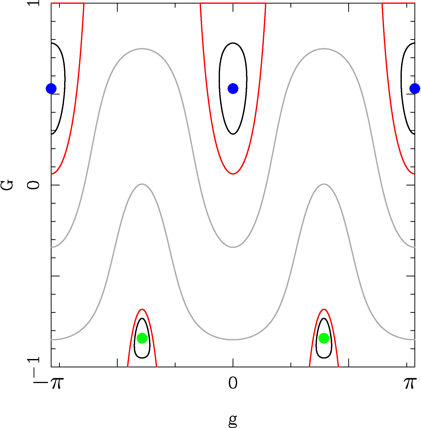
Figure 2: Phase portrait of ${\rm H}_{\rm slow}^{0}$ given in (25) with $C=25,\beta=\bar{\beta}=80$.

2 Euler problem revisited

In this section we review the classical integration of the two–centre problem and complement it with considerations that will be useful to us in the next.

The 2CP is the system, in ${\mathbb{R}}^{3}$ (or ${\mathbb{R}}^{2}$), of one particle interacting with two fixed masses via Newton Law. If $\pm{\mathbf{v}}_{0}\in{{{R}}}^{3}$ are the position coordinates of the centers, ${\rm m}_{\pm}$ their masses; ${\mathbf{v}}$, with ${\mathbf{v}}\neq\pm{\mathbf{v}}_{0}$, the position coordinate of the moving particle; ${\mathbf{u}}=\dot{\mathbf{v}}$ its velocity, and $1$ its mass, the Hamiltonian of the system (Euler Hamiltonian) is

$${\rm J}=\frac{\|{\mathbf{u}}\|^{2}}{2}-\frac{{\rm m}_{+}}{\|{\mathbf{v}}+{\mathbf{v}}_{0}\|}-\frac{{\rm m}_{-}}{\|{\mathbf{v}}-{\mathbf{v}}_{0}\|}\,.$$ (27)

Euler showed [13] that ${\rm J}$ exhibits $2$ independent first integrals, in involution. One of these first integrals is the projection

$$\Theta={\mathbf{M}}\cdot\frac{{\mathbf{v}}_{0}}{\|{\mathbf{v}}_{0}\|}$$ (28)

of the angular momentum ${\mathbf{M}}={\mathbf{v}}\times{\mathbf{u}}$ of the particle along the direction ${\mathbf{v}}_{0}$. It is not specifically due to the Newtonian potential, but, rather, to its invariance by rotations around the axis ${\mathbf{v}}_{0}$. For example, it persists if the Newtonian potential is replaced with a ${\alpha}$–homogeneous one. The existence of the following constant of motion, which we shall refer to as Euler integral:

$${\rm E}=\|{\mathbf{v}}\times{\mathbf{u}}\|^{2}+({\mathbf{v}}_{0}\cdot{\mathbf{u}})^{2}+2{\mathbf{v}}\cdot{\mathbf{v}}_{0}\left(\frac{{\rm m}_{+}}{\|{\mathbf{v}}+{\mathbf{v}}_{0}\|}-\frac{{\rm m}_{-}}{\|{\mathbf{v}}-{\mathbf{v}}_{0}\|}\right)$$ (29)

is pretty specific of ${\rm J}$. As observed in [3], in the limit of merging centers, i.e., ${\mathbf{v}}_{0}=\mathbf{0}$, ${\rm J}$ reduces to the Kepler Hamiltonian (5), and ${\rm E}$ to the squared length of the angular momentum of the moving particle.

The formula in (29) is not easy to be found in the literature, so we briefly discuss it.
After fixing a reference frame with the third axis in the direction of ${\mathbf{v}}_{0}$ and denoting as $(v_{1},v_{2},v_{3})$ the coordinates of ${\mathbf{v}}$ with respect to such frame, one introduces the so–called “elliptic coordinates”

$${\lambda}=\frac{1}{2}\left(\frac{{\rm r}_{+}}{{\rm r}_{0}}+\frac{{\rm r}_{-}}{{\rm r}_{0}}\right)\,,\quad{\beta}=\frac{1}{2}\left(\frac{{\rm r}_{+}}{{\rm r}_{0}}-\frac{{\rm r}_{-}}{{\rm r}_{0}}\right)\,,\quad{\omega}:=\arg{(-v_{2},v_{1})}\,,$$ (30)

where we have let, for short,

$${\rm r}_{0}:=\|{\mathbf{v}}_{0}\|\,,\quad{\rm r}_{\pm}:=\|{\mathbf{v}}\pm{\mathbf{v}}_{0}\|\,.$$

Regarding ${\rm r}_{0}$ as a fixed external parameter and calling $p_{\lambda}$, $p_{\beta}$, $p_{\omega}$ the generalized momenta associated to ${\lambda}$, ${\beta}$ and ${\omega}$, it turns out that the Hamiltonian (27), written in the coordinates $(p_{\lambda},p_{\beta},{\lambda},{\beta})$ is independent of ${\omega}$ and has the expression

$${\rm J}(p_{\lambda},p_{\beta},p_{\omega},{\lambda},{\beta},{\rm r}_{0}) = \frac{1}{{\lambda}^{2}-{\beta}^{2}}\Big{[}\frac{p^{2}_{\lambda}({\lambda}^{2}-1)}{2{\rm r}_{0}^{2}}+\frac{p^{2}_{\beta}(1-\beta^{2})}{2{\rm r}_{0}^{2}}+\frac{p_{\omega}^{2}}{2{\rm r}_{0}^{2}}\left(\frac{1}{1-\beta^{2}}\right.$$ (31)

$$\left.+\frac{1}{{\lambda}^{2}-1}\right)-\frac{({\rm m}_{+}+{\rm m}_{-}){\lambda}}{{\rm r}_{0}^{2}}+\frac{({\rm m}_{+}-{\rm m}_{-})\beta}{{\rm r}_{0}^{2}}\Big{]}\,.$$

It follows that the solution $W$ of Hamilton–Jacobi equation

$${\rm J}(W_{\lambda},W_{\beta},p_{\omega},{\lambda},{\beta},{\rm r}_{0})=h$$ (32)

can be searched of the form

$$W({\lambda},{\beta},p_{\omega},{\rm r}_{0},h)=W^{(1)}({\lambda},p_{\omega},{\rm r}_{0},h)+W^{(2)}({\beta},p_{\omega},{\rm r}_{0},h)$$

and (32) separates completely as

$${\cal F}^{(1)}(W^{(1)}_{\lambda},{\lambda},{p_{\omega}},{\rm r}_{0},h)+{\cal F}^{(2)}(W^{(2)}_{\beta},{\beta},{p_{\omega}},{\rm r}_{0},h)=0$$ (33)

with ${\cal F}^{(1)}$, ${\cal F}^{(2)}$ defined via (31)–(32).

The identity (33) implies that there must exist a function ${\rm E}$, which we call Euler integral, depending on $({p_{\omega}},{\rm r}_{0},h)$ only, such that

$${\cal F}^{(1)}(p_{\lambda},{\lambda},{p_{\omega}},{\rm r}_{0},h)=-{\cal F}^{(2)}(p_{\beta},{\beta},{p_{\omega}},{\rm r}_{0},h)={\rm E}({p_{\omega}},{\rm r}_{0},h)\quad\forall\ (p_{\lambda},p_{\beta},{\lambda},{\beta})\,.$$

After elementary computations, one find that, in terms of the initial position–impulse coordinates, the Euler Integral

$${\rm E}=\frac{1}{2}\left({\cal F}^{(1)}-{\cal F}^{(2)}\right)$$ (34)

has the expression in (29), when written in the original coordinates.

The “asymmetric” case

We are interested to find the expression of the Euler integral (29) when 2CP is written in the form

$${\rm J}=\frac{\|{{\mathbf{y}}}\|^{2}}{2}-\frac{1}{\|{\mathbf{x}}\|}-\frac{{\cal M}^{\prime}}{\|{\mathbf{x}}^{\prime}-{{\mathbf{x}}}\|}$$ (35)

namely, when the two centres are in “asymmetric positions”, $\mathbf{0}$, $\mathbf{x}^{\prime}$. As we shall see, in that case we have

$${\rm E}=\|{\mathbf{M}}\|^{2}-{\mathbf{x}}^{\prime}\cdot{\mathbf{L}}+{\cal M}^{\prime}\frac{({\mathbf{x}}^{\prime}-{\mathbf{x}})\cdot{\mathbf{x}}^{\prime}}{\|{\mathbf{x}}^{\prime}-{\mathbf{x}}\|}$$ (36)

where

$${\mathbf{M}}:={\mathbf{x}}\times{\mathbf{y}}\,,\qquad{\mathbf{L}}:={{\mathbf{y}}}\times{\mathbf{M}}-\frac{{{\mathbf{x}}}}{\|{{\mathbf{x}}}\|}={\rm e}{\mathbf{P}}$$ (37)

are the angular momentum and the eccentricity vector associated to the Kepler Hamiltonian (5) with ${\rm e}$ and ${\mathbf{P}}$ being the eccentricity and the perihelion direction ($\|{\mathbf{P}}\|=1$). Notice that ${\rm J}$ reduces to a Kepler Hamiltonian in two cases: either for ${\mathbf{x}}^{\prime}=\mathbf{0}$, in which case, as in the symmetric case above, ${\rm E}$ reduces to $\|{\mathbf{M}}\|^{2}$, or for ${\cal M}^{\prime}=0$. The latter case is more interesting to us, as ${\rm J}$ and ${\rm E}$ become, respectively, ${\rm J}_{0}$ in (5) and

$${\rm E}_{0} = \|{\mathbf{M}}\|^{2}-{\mathbf{x}}^{\prime}\cdot{\mathbf{L}}$$ (38)

with ${\rm E}_{0}$ being – as well expected – a combination of first integrals of ${\rm J}_{0}$.
To prove (36)–(37), we change, canonically,

$${\mathbf{x}}^{\prime}=2{\mathbf{v}}_{0}\,,\quad{\mathbf{x}}={\mathbf{v}}_{0}+{\mathbf{v}}\,,\quad{\mathbf{y}}^{\prime}=\frac{1}{2}({\mathbf{u}}_{0}-{\mathbf{u}})\,,\quad{\mathbf{y}}={\mathbf{u}}$$

(where ${\mathbf{y}}^{\prime}$, ${\mathbf{u}}_{0}$ denote the generalized impulses conjugated to ${\mathbf{x}}^{\prime}$, ${\mathbf{v}}_{0}$, respectively) we reach the Hamiltonian ${\rm J}$ in (27), with ${\rm m}_{+}=1$, ${\rm m}_{-}={\cal M}^{\prime}$. Turning back with the transformations, one sees that the function ${\rm E}$ in (29) takes the expression

$${{\rm E}} := \left\|\left({\mathbf{x}}-\frac{{\mathbf{x}}^{\prime}}{2}\right)\times{\mathbf{y}}\right\|^{2}+\frac{1}{4}({\mathbf{x}}^{\prime}\cdot{\mathbf{y}})^{2}+{\mathbf{x}}^{\prime}\cdot\left({\mathbf{x}}-\frac{{\mathbf{x}}^{\prime}}{2}\right)\left(\frac{1}{\|{\mathbf{x}}\|}-\frac{{\cal M}^{\prime}}{\|{\mathbf{x}}^{\prime}-{\mathbf{x}}\|}\right)\,.$$

and we rewrite it as

$${\rm E}={\rm E}_{0}+{\rm E}_{1}+{\rm E}_{2}$$

with

$${\rm E}_{0}:=\|{\mathbf{M}}\|^{2}-{\mathbf{x}}^{\prime}\cdot{\mathbf{L}}\,,\quad{\rm E}_{1}:={\cal M}^{\prime}\frac{({\mathbf{x}}^{\prime}-{\mathbf{x}})\cdot{\mathbf{x}}^{\prime}}{\|{\mathbf{x}}^{\prime}-{\mathbf{x}}\|}$$

$${\rm E}_{2}:=\frac{\|{\mathbf{x}}^{\prime}\|^{2}}{2}\left(\frac{\|{{\mathbf{y}}}\|^{2}}{2}-\frac{1}{\|{\mathbf{x}}\|}-\frac{{\cal M}^{\prime}}{\|{\mathbf{x}}^{\prime}-{{\mathbf{x}}}\|}\right)$$

where ${\mathbf{M}}$, ${\mathbf{L}}$ are as in (37). Since ${\rm E}_{2}$ is itself an integral for ${{\rm J}}$, we can neglect it and rename

$${\rm E}:={\rm E}_{0}+{\rm E}_{1}$$ (39)

the Euler integral to ${{\rm J}}$. Namely,

$$\Big{\{}{\rm J},{\rm E}\Big{\}}=0\,.$$ (40)

A set of canonical coordinates which lets ${\rm J}$ and ${\rm E}$ in 2 degrees–of–freedom

We describe a set of canonical coordinates, which we denote as ${\cal K}$, which we shall use for our analysis of the Euler Hamiltonian (35) and its integral ${\rm E}$ (39). This set of coordinates puts ${\rm J}$ and ${\rm E}$ in two degrees–of–freedom (represented by the couples $({\Lambda},\ell)$, $({\rm G},{\rm g})$ below), precisely like the classical ellipsoidal coordinates (30) do, both in the spatial and planar case.

We consider, in the region of $({\mathbf{y}},{\mathbf{x}})$ where ${\rm J}_{0}$ in (5) takes negative values and the ellipse ${\mathbb{E}}({\mathbf{y}},{\mathbf{x}})$ it generates starting from any initial datum $({\mathbf{y}},{\mathbf{x}})$ in this region is not a circle. Denote as:

• $a$ the semi–major axis;

• ${\mathbf{P}}$, with $\|{\mathbf{P}}\|=1$, the direction of perihelion, assuming the ellipse is not a circle;

• $\ell$: the mean anomaly, defined, mod $2{\pi}$, as the area of the elliptic sector spanned by ${\mathbf{x}}$ from ${\mathbf{P}}$, normalized to $2{\pi}$.

Finally,

• given three vectors ${\mathbf{u}}$, ${\mathbf{v}}$ and ${\mathbf{w}}$, with ${\mathbf{u}}$, ${\mathbf{v}}\perp{\mathbf{w}}$, we denote as ${\alpha}_{\mathbf{w}}({\mathbf{u}},{\mathbf{v}})$ the oriented angle from ${\mathbf{u}}$ to ${\mathbf{v}}$ relatively to the positive orientation established by ${\mathbf{w}}$.

We fix an arbitrary (“inertial”) frame

$${\rm F}_{0}:\qquad{\mathbf{i}}=\left(\begin{array}[]{lll}1\\ 0\\ 0\end{array}\right)\,,\qquad{\mathbf{j}}=\left(\begin{array}[]{lll}0\\ 1\\ 0\end{array}\right)\,,\qquad{\mathbf{k}}=\left(\begin{array}[]{lll}0\\ 0\\ 1\end{array}\right)$$

in ${{R}}^{3}$, and denote as

$${\mathbf{M}}={\mathbf{x}}\times{\mathbf{y}}\,,\quad{\mathbf{M}}^{\prime}={\mathbf{x}}^{\prime}\times{\mathbf{y}}^{\prime}\,,\quad{\mathbf{C}}={\mathbf{M}}^{\prime}+{\mathbf{M}}\,,$$

where “$\times$” denotes skew–product in ${{{R}}}^{3}$. Observe the following relations

$${{\mathbf{x}}^{\prime}}\cdot{{\mathbf{C}}}={{\mathbf{x}}^{\prime}}\cdot{\big{(}{\mathbf{M}}+{\mathbf{M}}^{\prime}\big{)}}={{\mathbf{x}}^{\prime}}\cdot{{\mathbf{M}}}\,,\qquad{\mathbf{P}}\cdot{\mathbf{M}}=0\,,\quad\|{\mathbf{P}}\|=1\,.$$ (42)

Assume that the “nodes”

$${\mathbf{n}}_{1}:={\mathbf{k}}\times{\mathbf{C}}\,,\quad{\mathbf{n}}_{2}:={\mathbf{C}}\times{\mathbf{x}}^{\prime}\,,\quad{\mathbf{n}}_{3}:={\mathbf{x}}^{\prime}\times{\mathbf{M}}$$ (43)

do not vanish. We define the coordinates

$${{\cal K}}=({\rm Z},{\rm C},\Theta,{\rm G},{\rm R},{\Lambda},\zeta,g,\vartheta,{\rm g},{\rm r},\ell)$$

via the following formulae.

$$\left\{\begin{array}[]{l}\displaystyle{\rm Z}:={\mathbf{C}}\cdot{\mathbf{k}}\\ \\ \displaystyle{\rm C}:=\|{\mathbf{C}}\|\\ \\ \displaystyle{\rm R}:=\frac{{\mathbf{y}}^{\prime}\cdot{\mathbf{x}}^{\prime}}{\|{\mathbf{x}}^{\prime}\|}\\ \\ \displaystyle{\Lambda}=\sqrt{a}\\ \\ \displaystyle{\rm G}:=\|{\mathbf{M}}\|\\ \\ \displaystyle\Theta:=\frac{{\mathbf{M}}\cdot{\mathbf{x}}^{\prime}}{\|{\mathbf{x}}^{\prime}\|}\\ \end{array}\right.\qquad\qquad\left\{\begin{array}[]{l}\displaystyle{\rm z}:={\alpha}_{{\mathbf{k}}}({\mathbf{i}},{\mathbf{n}}_{1})\\ \\ \displaystyle g:={\alpha}_{{\mathbf{C}}}({\mathbf{n}}_{1},{\mathbf{n}}_{2})\\ \\ \displaystyle{\rm r}:=\|{\mathbf{x}}^{\prime}\|\\ \\ \ell:=\textrm{\rm mean anomaly of }{\mathbf{x}}\ {\rm on\ \mathbb{E}}\\ \\ {\rm g}:={\alpha}_{{\mathbf{M}}}({\mathbf{n}}_{3},{\mathbf{M}}\times{\mathbf{P}})\\ \\ \displaystyle\vartheta:={\alpha}_{{\mathbf{x}}^{\prime}}({\mathbf{n}}_{2},{\mathbf{n}}_{3})\end{array}\right.$$ (66)

The canonical character of ${{\cal K}}$ has been discussed in [17]. In the planar case, the coordinates (66) reduce to the 8 coordinates

$$\left\{\begin{array}[]{l}\displaystyle{\rm C}=\|{\mathbf{x}}\times{\mathbf{y}}+{\mathbf{x}}^{\prime}\times{\mathbf{y}}^{\prime}\|\\ \\ \displaystyle{\rm G}=\|{\mathbf{x}}\times{\mathbf{y}}\|\\ \\ \displaystyle{\rm R}=\frac{\mathbf{y}^{\prime}\cdot\mathbf{x}^{\prime}}{\|\mathbf{x}^{\prime}\|}\\ \\ \displaystyle{\Lambda}=\sqrt{a}\end{array}\right.\qquad\qquad\left\{\begin{array}[]{l}\displaystyle{\gamma}={\alpha}_{\mathbf{k}}(\mathbf{i},\mathbf{x}^{\prime})+\frac{{\pi}}{2}\\ \\ \displaystyle{\rm g}={\alpha}_{\mathbf{k}}({\mathbf{x}^{\prime}},\mathbf{P})+{\pi}\\ \\ \displaystyle{\rm r}=\|\mathbf{x}^{\prime}\|\\ \\ \displaystyle\ell={\rm mean\ anomaly\ of\ {\mathbf{x}}\ in\ \mathbb{E}}\end{array}\right.$$ (81)

Using the formulae in the previous section, we provide the expressions of ${\rm J}$ in (35) and and ${\rm E}$ in (38) in terms of ${{\cal K}}$:

$${\rm J}({\Lambda},{\rm G},\Theta,{\rm r},\ell,{\rm g}) = -\frac{1}{2{\Lambda}^{2}}-\frac{{\cal M}^{\prime}}{\sqrt{{{\rm r}}^{2}+2{\rm r}a\sqrt{1-\frac{\Theta^{2}}{{\rm G}^{2}}}{\rm p}+{a}^{2}\varrho^{2}}}$$

$$=: {\rm J}_{0}+{\rm J}_{1}$$

$${\rm E}({\Lambda},{\rm G},\Theta,{\rm r},\ell,{\rm g}) = {\rm G}^{2}+{\rm r}\sqrt{1-\frac{\Theta^{2}}{{\rm G}^{2}}}\sqrt{1-\frac{{\rm G}^{2}}{{\Lambda}^{2}}}\cos{\rm g}$$ (82)

$$+ {\cal M}^{\prime}{\rm r}\frac{{{\rm r}}+a\sqrt{1-\frac{\Theta^{2}}{{\rm G}^{2}}}{\rm p}}{\sqrt{{{\rm r}}^{2}+2{\rm r}a\sqrt{1-\frac{\Theta^{2}}{{\rm G}^{2}}}{\rm p}+{a}^{2}\varrho^{2}}}$$

$$=: {\rm E}_{0}+{\rm E}_{1}$$

and, if $\xi=\xi({\Lambda},{\rm G},\ell)$ is the eccentric anomaly, defined as the solution of Kepler equation

$$\xi-{\rm e}({\Lambda},{\rm G})\sin\xi=\ell$$ (83)

and $a=a({\Lambda})$ the semi–major axis; ${\rm e}={\rm e}({\Lambda},{\rm G})$, the eccentricity of the ellipse, $\varrho=\varrho({\Lambda},{\rm G},\ell)$, ${\rm p}={\rm p}({\Lambda},{\rm G},\ell,{\rm g})$ are defined as

$$a({\Lambda}) = {{\Lambda}^{2}}$$

$${\rm e}({\Lambda},{\rm G}) := \sqrt{1-\frac{{\rm G}^{2}}{{\Lambda}^{2}}}$$

$$\varrho({\Lambda},{\rm G},\ell) := 1-{\rm e}({\Lambda},{\rm G})\cos\xi({\Lambda},{\rm G},\ell)$$

$${\rm p}({\Lambda},{\rm G},\ell,{\rm g}) := (\cos\xi({\Lambda},{\rm G},\ell)-{\rm e}({\Lambda},{\rm G}))\cos{\rm g}-\frac{{\rm G}}{{\Lambda}}\sin\xi({\Lambda},{\rm G},\ell)\sin{\rm g}\,.$$ (84)

The angle

$${\nu}({\Lambda},{\rm G},\ell):=\arg\left(\cos\xi({\Lambda},{\rm G},\ell)-{\rm e}({\Lambda},{\rm G}),\frac{{\rm G}}{{\Lambda}}\sin\xi({\Lambda},{\rm G},\ell)\right)$$ (85)

is usually referred to as true anomaly, so one recognises that ${\rm p}({\Lambda},{\rm G},\ell,{\rm g})=\varrho\cos({\nu}+{\rm g})$.

Observe that ${\rm E}$ and ${\rm J}$ in (2) do not depend on ${\rm C}$, ${\rm Z}$, $\zeta$, ${\gamma}$, ${\rm R}$, $\vartheta$, while the Hamiltonians (1), do not depend on ${\rm Z}$, $\zeta$, ${\gamma}$, $\ell$.

The details on the derivation of the formulae in (2) may be found in [17].

Renormalizable integrability

In this section we review the property of renormalizable integrability pointed out in [16].

We consider the function ${\rm U}_{\beta}$ in (8) with ${\beta}=1$, which is given by

$${\rm U}({\rm r},{\Lambda},\Theta,{\rm G},{\rm g})=\frac{1}{2{\pi}}\int_{0}^{2{\pi}}\frac{d\ell}{\sqrt{{{\rm r}}^{2}+2{\rm r}a\sqrt{1-\frac{\Theta^{2}}{{\rm G}^{2}}}{\rm p}+{a}^{2}\varrho^{2}}}$$ (86)

and the function

$${\rm E}_{0}={\rm G}^{2}+{\rm r}\sqrt{1-\frac{\Theta^{2}}{{\rm G}^{2}}}\sqrt{1-\frac{{\rm G}^{2}}{{\Lambda}^{2}}}\cos{\rm g}$$

in (2). These two functions have the following remarkable properties:

• they have one effective degree–of–freedom, as they depend on one conjugated couple of coordinates: the couple $({\rm G},{\rm g}$);

• they Poisson–commute:

  $$\Big{\{}{\rm U},\ {\rm E}_{0}\Big{\}}=0\,.$$ (87)

Relation (87) can be proved taking the $\ell$–average of (40), and exploiting that ${\rm J}_{0}$ depends only on ${\Lambda}$; see [16]. The following definition relies precisely with this situation.

Definition 2.1 ([16]).

Let $h$, $g$ be two functions of the form

$$h(p,q,y,x)=\mathaccent 866{h}({\rm I}(p,q),y,x)\,,\qquad g(p,q,y,x)=\mathaccent 866{g}({\rm I}(p,q),y,x)$$ (88)

where

$$(p,q,y,x)\in{\cal D}:={\cal B}\times U$$ (89)

with $U\subset{{R}}^{2}$, ${\cal B}\subset{{R}}^{2n}$ open and connected, $(p,q)=$ $(p_{1}$, $\cdots$, $p_{n}$, $q_{1}$, $\cdots$, $q_{n})$ conjugate coordinates with respect to the two–form ${\omega}=dy\wedge dx+\sum_{i=1}^{n}dp_{i}\wedge dq_{i}$ and ${\rm I}(p,q)=({\rm I}_{1}(p,q),\cdots,{\rm I}_{n}(p,q))$, with

$${\rm I}_{i}:\ {\cal B}\to{{R}}\,,\qquad i=1,\cdots,n$$

pairwise Poisson commuting:

$$\big{\{}{\rm I}_{i},{\rm I}_{j}\big{\}}=0\qquad\forall\ 1\leq i<j\leq n\qquad i=1,\cdots,n\,.$$ (90)

We say that $h$ is renormalizably integrable via $g$ if there exists a function

$$\mathaccent 869{h}:\qquad{\rm I}({\cal B})\times g(U)\to{{R}}\,,$$

such that

$$h(p,q,y,x)=\mathaccent 869{h}({\rm I}(p,q),\mathaccent 866{g}({\rm I}(p,q),y,x))$$ (91)

for all $(p,q,y,x)\in{\cal D}$.

Proposition 2.2 ([16]).

If $h$ is renormalizably integrable via $g$, then:

${\rm I}_{1}$, $\cdots$, ${\rm I}_{n}$ are first integrals to $h$ and $g$;

$h$ and $g$ Poisson commute.

Proposition 2.3 ([16]).

${\rm U}$ is renormalizably integrable via ${\rm E}_{0}$. Namely, there exists a function ${\rm F}$ such that

$${\rm U}({\rm r},{\Lambda},\Theta,{\rm G},{\rm g})={\rm F}\big{(}{\rm r},{\Lambda},\Theta,{\rm E}_{0}({\rm r},{\Lambda},\Theta,{\rm G},{\rm g})\big{)}\,.$$

The proof of Proposition 2.3 is based on ${\cal P}_{1}\div{\cal P}_{2}$ above. Below, we list some consequences.

• If ${\rm F}_{{\rm E}_{0}}\neq 0$, the time laws of $({\rm G},{\rm g})$ under ${\rm U}$ or ${\rm E}_{0}$ are basically (i.e., up to a change of time) the same;

• Motions of ${\rm E}_{0}$ corresponding to level sets for which ${\rm F}_{{\rm E}_{0}}=0$ are fixed points curves to ${\rm U}$ (“frozen orbits”). In [16] we provided an example of frozen orbit of ${\rm U}$ in the spatial case, for ${\rm r}\ll 1$;

• ${\rm U}$ and ${\rm E}_{0}$ have the same action–angle coordinates;

• ${\rm F}$ may have several expressions, as well as ${\rm U}$, which is defined via a quadrature. Two different representation formulae have been proposed in [16] and [18].

In the next section, we investigate the dynamical properties of ${\rm E}_{0}$ for the planar case ($\Theta=0$).

The phase portrait of ${\rm E}_{0}$ in the planar case

Here we fix ${\Lambda}=1$, $\Theta=0$. For ${\rm r}\in(0,2)$, the function ${\rm E}_{0}({\rm g},{\rm G})$ has a minimum, a saddle and a maximum, respectively at

$${\mathbf{P}}_{-}=(\pm{\pi},0)\,,\qquad{\mathbf{P}}_{0}=(0,0)\,,\qquad{\mathbf{P}}_{+}=\left(0,\sqrt{1-\frac{{\rm r}^{2}}{4}}\right)$$

where it takes the values, respectively,

$${\cal E}_{-}=-{\rm r}\,,\qquad{\cal E}_{0}={\rm r}\,,\quad{\cal E}_{+}=1+\frac{{\rm r}^{2}}{4}\,.$$

Thus, the level sets in (12) are non–empty only for

$${\cal E}\in\left[-{\rm r},1+\frac{{\rm r}^{2}}{4}\right]\,.$$ (92)

We denote as ${\cal S}_{0}$, the level set through the saddle ${\mathbf{P}}_{0}$. When ${\rm G}=1$, ${\rm E}_{0}$ takes the value $1$ for all ${\rm g}$ and we denote as ${\cal S}_{1}$ the level curve with ${\cal E}=1$. The equations of ${\cal S}_{0}$, ${\cal S}_{1}$ are, respectively:

$${\cal S}_{0}({\rm r})=\Big{\{}({\rm g},{\rm G}):\ {\rm G}^{2}+{\rm r}\sqrt{1-{\rm G}^{2}}\cos{\rm g}={\rm r}\Big{\}},$$

$${\cal S}_{1}({\rm r})=\Big{\{}{\rm G}=\pm 1\Big{\}}\cup\Big{\{}{\rm G}=\pm\sqrt{1-{\rm r}^{2}\cos^{2}{\rm g}}\Big{\}}.$$ (93)

${\cal S}_{1}$ is composed of two branches, which will be referred to as “horizontal”, “vertical”, respectively, transversally intersecting at $(\pm\frac{{\pi}}{2},1)$, with ${\rm g}$ mod $2{\pi}$. Note that, when $0<{\rm r}<1$, the vertical branch is defined for all ${\rm g}\in{{T}}$; when ${\rm r}>1$, its domain in ${\rm g}$ is made of two disjoint neighbourhoods of $\pm\frac{{\pi}}{2}$.
When ${\rm r}>2$, the saddle ${\mathbf{P}}_{0}$ and its manifold ${\cal S}_{0}$ do not exist, ${\mathbf{P}}_{-}=({\pi},0)$ is still a minimum, while the maximum becomes ${\mathbf{P}}_{+}=(0,0)$. The manifold ${\cal S}_{1}$ still exists, with the vertical branch closer and closer, as ${\rm r}\to+\infty$, to the portion of straight ${\rm g}=\pm\frac{{\pi}}{2}$ in the strip $-1\leq{\rm G}\leq 1$. In this case the admissible values for ${\cal E}$ are

$${\cal E}\in\left[-{\rm r},{\rm r}\right]\,.$$

It is worth mentioning [17] that, when $0<{\rm r}<2$, the motions generated by ${\rm E}_{0}$ along ${\cal S}_{0}({\rm r})$ can be explicitly computed, and are given by

$$\left\{\begin{array}[]{l}{\rm G}(t)=\frac{{\sigma}{\Lambda}}{\cosh{\sigma}{\Lambda}(t-t_{0})},\\ \\ \displaystyle{\rm g}(t)=\pm\cos^{-1}\frac{1-\frac{{\alpha}^{2}}{\cosh^{2}{\sigma}{\Lambda}(t-t_{0})}}{\sqrt{1-\frac{{\sigma}^{2}}{\cosh^{2}{\sigma}{\Lambda}(t-t_{0})}}}\,,\end{array}\right.$$

where

$${\sigma}^{2}:={\rm r}(2-{\rm r})\,,\quad{\alpha}^{2}:=2-{\rm r}\,,\quad{\rm r}\in(0,2)\,.$$ (95)

These motions – which have a remarkable similitude with the separatrix motions of the classical pendulum – are however meaningless for ${\rm U}$, which is singular on ${\cal S}_{0}({\rm r})$.

The scenario is depicted in Figure 1 to which we refer for further qualitative details.

3 Perihelion librations in the three–body problem

In this section we review the results of [16], [18], [17].

As mentioned in the introduction, the proof of Theorem 1.1 is based on two ingredients: a normal form theory well designed around the Hamiltonians (1), where no non–resonance condition is required, and a set of action–angle–like coordinates which approximate well the natural action–angle coordinates of ${\rm E}_{0}$ when ${\rm r}$ is large. In this section we briefly summarise the procedure. Full details may be found in [18].

A normal form theory without small divisors

We describe a procedure for eliminating the angles $\bm{{\varphi}}$ at high orders, given Hamiltonian of the form

$${\rm H}({\mathbf{I}},\bm{{\varphi}},{\mathbf{p}},{\mathbf{q}},y,x)={\rm h}({\mathbf{I}},{\mathbf{J}}({\mathbf{p}},{\mathbf{q}}),y)+f({\mathbf{I}},\bm{{\varphi}},{\mathbf{p}},{\mathbf{q}},y,x)$$ (96)

which we assume to be holomorphic on the neighbourhood

$${\mathbb{P}}_{{\rho},s,{\delta},r,\xi}={\mathbb{I}}_{\rho}\times{{\mathbb{T}}}^{n}_{s}\times{\mathbb{B}}_{{\delta}}\times{\mathbb{Y}}_{r}\times{\mathbb{X}}_{\xi}\supset{\mathbb{P}}={\mathbb{I}}\times{{\mathbb{T}}}^{n}\times{\mathbb{B}}\times{\mathbb{Y}}\times{\mathbb{X}}\,,$$

for suitable ${\rho}$, $s$, ${\delta}$, $r$, $\xi>0$ and

$${\mathbf{J}}({\mathbf{p}},{\mathbf{q}})=(p_{1}q_{1},\cdots,p_{m}q_{m})\,.$$

Here, ${\mathbb{I}}\subset{\mathbb{R}}^{n}$, ${\mathbb{B}}\subset{\mathbb{R}}^{2m}$, ${\mathbb{Y}}\subset{\mathbb{R}}$, ${\mathbb{X}}\subset{\mathbb{R}}$ are open and connected; $\mathbb{T}=\mathbb{R}/(2{\pi}\mathbb{Z})$ is the standard torus, and we have used the common notation $A_{r}:=\bigcup_{x\in A}B_{r}(x)$, where $B_{r}(x)$ is the complex open ball centered in $x$ with radius $r$.

We denote as ${\cal O}_{{\rho},s,{\delta},r,\xi}$ the set of complex holomorphic functions

$$\phi:\quad{\mathbb{P}}_{\hat{\rho},\hat{s},\hat{\delta},\hat{r},\hat{\xi}}\to{{{C}}}$$

for some $\hat{\rho}>{\rho}$, $\hat{s}>s$, $\hat{\delta}>{\delta}$, $\hat{r}>r$, $\hat{\xi}>\xi$, equipped with the norm

$$\|\phi\|_{{\rho},s,{\delta},r,\xi}:=\sum_{k,h,j}\|\phi_{khj}\|_{{\rho},r,\xi}e^{s|k|}{\delta}^{h+j}$$

where $\phi_{khj}({\mathbf{I}},y,x)$ are the coefficients of the Taylor–Fourier expansion

$$\phi=\sum_{k,h,j}\phi_{khj}({\mathbf{I}},y,x)e^{{\rm i}ks}{\mathbf{p}}^{h}{\mathbf{q}}^{j}\,,\quad\|\phi\|_{{\rho},r,\xi}:=\sup_{{\mathbb{I}}_{\rho}\times{\mathbb{Y}}_{r}\times{\mathbb{X}}_{\xi}}|\phi({\mathbf{I}},y,x)|\,.$$

If $\phi$ is independent of $x$, we simply write $\|\phi\|_{{\rho},r}$ for $\|\phi\|_{{\rho},r,\xi}$. If $\phi\in{\cal O}_{{\rho},s,{\delta},r,\xi}$, we define its “off–average” $\mathaccent 869{\phi}$ and “average” $\overline{\phi}$ as

$$\mathaccent 869{\phi}:=\sum_{k,h,j:\atop(k,h-j)\neq(0,0)}\phi_{khj}({\mathbf{I}},y,x)e^{{\rm i}ks}{\mathbf{p}}^{h}{\mathbf{q}}^{j}$$

$$\overline{\phi}:=\phi-\mathaccent 869{\phi}=\frac{1}{(2{\pi})^{n}}\int_{[0,2{\pi}]^{n}}{\Pi}_{{\mathbf{p}}\mathbf{q}}\phi({\mathbf{I}},\bm{{\varphi}},{\mathbf{J}}({\mathbf{p}},{\mathbf{q}}),y,x)d\bm{{\varphi}}\,,$$

with

$${\Pi}_{{\mathbf{p}}\mathbf{q}}\phi({\mathbf{I}},\bm{{\varphi}},{\mathbf{J}}({\mathbf{p}},{\mathbf{q}}),y,x):=\sum_{k,h}\phi_{khh}({\mathbf{I}},y,x)e^{{\rm i}ks}{\mathbf{p}}^{h}{\mathbf{q}}^{h}$$

We decompose

$${\cal O}_{{\rho},s,{\delta},r,\xi}={\cal Z}_{{\rho},s,{\delta},r,\xi}\oplus{\cal N}_{{\rho},s,{\delta},r,\xi}\,.$$

where ${\cal Z}_{{\rho},s,{\delta},r,\xi}$, ${\cal N}_{{\rho},s,{\delta},r,\xi}$ are the “zero–average” and the “normal” classes

$${\cal Z}_{{\rho},s,{\delta},r,\xi}:=\{\phi\in{\cal O}_{{\rho},s,{\delta},r,\xi}:\quad\phi=\mathaccent 869{\phi}\}=\{\phi\in{\cal O}_{{\rho},s,{\delta},r,\xi}:\quad\overline{\phi}=0\}$$ (97)

$${\cal N}_{{\rho},s,{\delta},r,\xi}:=\{\phi\in{\cal O}_{{\rho},s,{\delta},r,\xi}:\quad\phi=\overline{\phi}\}=\{\phi\in{\cal O}_{{\rho},s,{\delta},r,\xi}:\quad\mathaccent 869{\phi}=0\}\,.$$ (98)

respectively. We finally let $\omega_{y,{\mathbf{I}},{\mathbf{J}}}:=\partial_{y,{\mathbf{I}},{\mathbf{J}}}{\rm h}$.

In the following result, no non–resonance condition is required on the frequencies ${\omega}_{\mathbf{I}}$, which, as a matter of fact, might also be zero.

Theorem 3.1 ([18]).

For any $n$, $m$, there exists a number ${\rm c}_{n,m}\geq 1$ such that, for any $N\in{\mathbb{N}}$ such that the following inequalities are satisfied

$$4N{\cal X}\left\|{\,\rm Im\,}\frac{{\omega}_{\mathbf{I}}}{{\omega}_{y}}\right\|_{{\rho},r}<s\,,\quad 4N{\cal X}\left\|\frac{{\omega}_{\mathbf{J}}}{{\omega}_{y}}\right\|_{{\rho},r}<1$$

$${\mathaccent 869{\rm c}_{n,m}N\frac{{\cal X}}{{\rm d}}\left\|{f}\right\|_{{\rho},s,{\delta},r,\xi}\left\|\frac{1}{{\omega}_{y}}\right\|_{{\rho},s,{\delta},r,\xi}<1}$$ (99)

with ${\rm d}:=\min\big{\{}{\rho}s,r\xi,{{\delta}}^{2}\big{\}}$, ${\cal X}:=\sup\big{\{}|x|:\ x\in{\mathbb{X}}_{\xi}\big{\}}$, one can find an operator

$$\Psi_{*}:\quad{\cal O}_{{\rho},s,{\delta},r,\xi}\to{\cal O}_{1/3({\rho},s,{\delta},r,\xi)}$$ (100)

which carries ${\rm H}$ to

$${\rm H}_{*}={\rm h}+g_{*}+f_{*}$$

where $g_{*}\in{\cal N}_{1/3({\rho},s,{\delta},r,\xi)}$, $f_{*}\in{\cal O}_{1/3({\rho},s,{\delta},r,\xi)}$ and, moreover, the following inequalities hold

$$\|g_{*}-\overline{f}\|_{1/3({\rho},s,{\delta},r,\xi)}\leq 162\mathaccent 869{\rm c}_{n,m}\frac{{\cal X}}{\rm d}\left\|{\frac{\mathaccent 869{f}}{{\omega}_{y}}}\right\|_{{\rho},s,{\delta},r,\xi}\|f\|_{{\rho},s,{\delta},r,\xi}$$

$$\|f_{*}\|_{1/3({\rho},s,{\delta},r,\xi)}\leq\frac{1}{2^{N+1}}\|f\|_{{\rho},s,{\delta},r,\xi}\,.$$ (101)

The transformation $\Psi_{*}$ can be obtained as a composition of time–one Hamiltonian flows, and satisfies the following. If

$$({\mathbf{I}},\bm{{\varphi}},{\mathbf{p}},{\mathbf{q}},y,x):=\Psi_{*}({\mathbf{I}}_{*},\bm{{\varphi}}_{*},{\mathbf{p}}_{*},{\mathbf{q}}_{*},{\rm R}_{*},{\rm r}_{*})$$

the following uniform bounds hold:

$${\rm d}\max\Big{\{}\frac{|{\mathbf{I}}-{\mathbf{I}}_{*}|}{{\rho}},\ \frac{|\bm{{\varphi}}-\bm{{\varphi}}_{*}|}{s},\ \frac{|{\mathbf{p}}-{\mathbf{p}}_{*}|}{{\delta}},\ \frac{|{\mathbf{q}}-{\mathbf{q}}_{*}|}{{\delta}},\ \frac{|y-y_{*}|}{r},\frac{|x-x_{*}|}{\xi}\Big{\}}$$

$$\leq\max\Big{\{}s|{\mathbf{I}}-{\mathbf{I}}_{*}|,\ {\rho}|\bm{{\varphi}}-\bm{{\varphi}}_{*}|,\ {\delta}|{\mathbf{p}}-{\mathbf{p}}_{*}|,\ {\delta}|{\mathbf{q}}-{\mathbf{q}}_{*}|,\ \xi|y-y_{*}|,\ r|x-x_{*}|\Big{\}}$$

$$\leq{{19\,{\cal X}\left\|\frac{f}{{\omega}_{y}}\right\|_{{\rho},s,{\delta},r,\xi}}}\,.$$ (102)

Hints on the proof of Theorem 3.1 may be found in Appendix A.

Asymptotic action–angle coordinates

The explicit construction of the action–angle coordinates for ${\rm E}_{0}$ for any value of ${\rm r}$ and $\Theta$ exhibits elliptic integrals. This is true even in the case $\Theta=0$, in which the phase portrait is, as discussed, explicit. As we are interested to the case that ${\rm r}$ is large, we adopt the “approximate” solution of integrating only the leading part of ${\rm E}$. Namely, we replace equation (12) with

$$\sqrt{1-{\rm G}^{2}}\cos{\rm g}=\mathaccent 869{{\cal E}}\,.$$ (103)

We show that, for this case, the action–angle coordinates, denoted as $({\cal G},{\gamma})$, are given by

$${\cal G}=\mathaccent 869{{\cal E}}\,,\quad{\gamma}={\tau}$$ (104)

where ${\tau}$ is the time the flows employs to reach the value $({\rm G},{\rm g})$ on the level set $\mathaccent 869{{\cal E}}$, starting from $(\sqrt{1-\mathaccent 869{{\cal E}}^{2}},0)$ ($(\sqrt{1-\mathaccent 869{{\cal E}}^{2}},{\pi})$). Namely, for the Hamiltonian (103), the action–angle coordinates coincide with the energy–time coordinates. Indeed, by (103), the action variable can be taken to be

$${\cal G}(\mathaccent 869{{\cal E}}) = \left\{\begin{array}[]{l}\displaystyle-1+\frac{1}{{\pi}}\int_{-\arccos|\mathaccent 869{{\cal E}}|}^{\arccos|\mathaccent 869{{\cal E}}|}\sqrt{1-\frac{\mathaccent 869{{\cal E}}^{2}}{\cos^{2}{\rm g}}}d{\rm g}\quad-1<\mathaccent 869{{\cal E}}<0\\ \\ \displaystyle 1-\frac{1}{{\pi}}\int_{-\arccos\mathaccent 869{{\cal E}}}^{\arccos\mathaccent 869{{\cal E}}}\sqrt{1-\frac{\mathaccent 869{{\cal E}}^{2}}{\cos^{2}{\rm g}}}d{\rm g}\quad 0<\mathaccent 869{{\cal E}}<1\,.\end{array}\right.$$

We have defined ${\cal G}(\mathaccent 869{{\cal E}})$ so that ${\cal G}(0)=0$. Then the period of the orbit is given by

$${\cal T}(\mathaccent 869{{\cal E}})=2{\pi}{\cal G}_{\mathaccent 869{{\cal E}}}(\mathaccent 869{{\cal E}})\,.$$

With the change of variable

$$w=\frac{|\mathaccent 869{{\cal E}}|}{\sqrt{1-\mathaccent 869{{\cal E}}^{2}}}\tan{\rm g}\,,$$ (106)

we obtain

$${\cal T}(\mathaccent 869{{\cal E}}) = 4|\mathaccent 869{{\cal E}}|\int_{0}^{\arccos|\mathaccent 869{{\cal E}}|}\frac{1}{\cos^{2}{\rm g}}\frac{d{\rm g}}{\sqrt{1-\frac{\mathaccent 869{{\cal E}}^{2}}{\cos^{2}{\rm g}}}}=4\int_{0}^{1}\frac{dw}{\sqrt{1-w^{2}}}=2{\pi}$$

which implies (104).
Looking at the (multi–valued) generating function

$$S({\cal G},{\rm g})=\int_{P_{0}({\cal G})}^{P_{\rm g}({\cal G})}\sqrt{1-\frac{{\cal G}^{2}}{\cos^{2}{\rm g}^{\prime}}}d{\rm g}^{\prime}$$

(where, as it is standard to do [1], the integral is computed along the ${\cal G}$th level set, from $P_{0}({\cal G}):=(-\arccos{\cal G},0)$ to a prefixed point $P_{\rm g}({\cal G})=({\rm g},\cdot)$ of the level set, so as to make $S({\cal G},\cdot)$ continuous) we obtain the transformation of coordinates

$$\left\{\begin{array}[]{l}\displaystyle{\rm G}=\sqrt{1-{\cal G}^{2}}\cos{\gamma}\\ \\ \displaystyle{\rm g}=-\tan^{-1}\left(\frac{1}{{\cal G}}\sqrt{1-{{\cal G}^{2}}}\sin{\gamma}\right)+k{\pi}\\ \\ {\rm with}\quad k=\left\{\begin{array}[]{l}0\ \ {\rm if}\ 0<{\cal G}<1\\ 1\ \ {\rm if}\ -1<{\cal G}<0\,.\end{array}\right.\end{array}\right.$$ (114)

Then, using the coordinates $({\cal G},{\gamma})$, one obtains the expression

$${\rm E}_{0}={{\cal G}}\,{\rm r}+(1-{\cal G}^{2})\cos^{2}{\gamma}$$

which will be used in the next section.

The proof of Theorem 1.1 is a direct application of Proposition 3.1. As such, a careful evaluation of the involved quantities is needed. Those evaluations are completely explicit in [18]. For the purpose of this review, we report below the main ideas while we skip most of computational details. The reader who is interested in them might consult [18].

Sketch of proof of Theorem 1.1

For definiteness, we sketch the proof of Theorem 1.1 for $(0,0)$. The proof for $(0,{\pi})$ is similar. For the purposes of this proof, we let $\mathaccent 866{{\rm H}}_{1}:=\mathaccent 866{{\rm H}}_{\rm J}$ and $\mathaccent 866{{\rm H}}_{2}:=\mathaccent 866{{\rm H}}_{0}$, where $\mathaccent 866{{\rm H}}_{\rm J}$ and $\mathaccent 866{{\rm H}}_{\rm J}$ are as in (1). It is convenient to rewrite the functions $\mathaccent 866{{\rm H}}_{i}$ as

$$\mathaccent 866{{\rm H}}_{1}({\rm R},{\rm G},{\rm r},{\rm g}) = \left(\frac{{\rm R}^{2}}{2}-\frac{1}{{\rm r}}\right)+\frac{{\rm G}^{2}}{2{\rm r}^{2}}-\frac{\overline{{\beta}}}{{\beta}+\overline{{\beta}}}\frac{1}{{\rm r}}\left(\mathaccent 866{{\rm F}}_{{\beta}\varepsilon({\rm r})}\Big{(}\mathaccent 866{{\rm E}}_{{\beta}\varepsilon({\rm r})}({\rm G},{\rm g})\Big{)}-1\right)$$

$$-\frac{{\beta}}{{\beta}+\overline{{\beta}}}\frac{1}{{\rm r}}\left(\mathaccent 866{{\rm F}}_{-\overline{{\beta}}\varepsilon({\rm r})}\Big{(}\mathaccent 866{{\rm E}}_{-\overline{{\beta}}\varepsilon({\rm r})}({\rm G},{\rm g})\Big{)}-1\right)$$

$$\mathaccent 866{{\rm H}}_{2}({\rm R},{\rm G},{\rm r},{\rm g}) = \left(\frac{{\rm R}^{2}}{2}-\frac{1}{{\rm r}}\right)+\frac{{\rm G}^{2}}{2{\rm r}^{2}}-\frac{\overline{{\beta}}}{{\beta}+\overline{{\beta}}}\frac{1}{{\rm r}}\left(\mathaccent 866{{\rm F}}_{({\beta}+\overline{{\beta}})\varepsilon({\rm r})}\Big{(}\mathaccent 866{{\rm E}}_{({\beta}+\overline{{\beta}})\varepsilon({\rm r})}({\rm G},{\rm g})\Big{)}-1\right)$$

where

$$\varepsilon({\rm r}):=\frac{1}{{{\rm r}}}\,,\quad\mathaccent 866{{\rm E}}_{\varepsilon}({\rm G},{\rm g}):=\varepsilon{\rm E}_{0}(\varepsilon^{-1},{\rm G},{\rm g})\,,\quad\mathaccent 866{{\rm F}}_{\varepsilon}(t):=\varepsilon^{-1}\,{\rm F}(\varepsilon^{-1},\varepsilon^{-1}t)\,.$$

We next change coordinates via the canonical changes

$${\cal C}_{1}:\ ({\cal G},{\gamma})\to({\rm G},{\rm g})\,,\quad{\cal C}_{2}:\ (y,x)\to({\rm R},{\rm r})$$

where ${\cal C}_{1}$ is defined as in (114), with $k=0$, while ${\cal C}_{2}$ is

$$\left\{\begin{array}[]{l}\displaystyle{\rm R}(y,x)=\frac{1}{y}\sqrt{\frac{\cos{\xi}^{\prime}(x)+1}{1-\cos\xi^{\prime}(x)}}\\ \\ \displaystyle{\rm r}(y,x)=y^{2}(1-\cos\xi^{\prime}(x))\end{array}\right.$$ (118)

where $\xi^{\prime}(x)$ solves

$$\xi^{\prime}-\sin\xi^{\prime}=x\,.$$ (119)

${\cal C}_{2}$ has been chosen so that

$$\left(\frac{{\rm R}^{2}}{2}-\frac{1}{{\rm r}}\right)\circ{\cal C}_{2}=-\frac{1}{2y^{2}}\,.$$

Using the new coordinates, we have

$$\mathaccent 866{{\rm H}}_{1} = -\frac{1}{2y^{2}}+\frac{1}{{\rm r}(y,x)}\left(\varepsilon(y,x)\frac{(1-{\cal G}^{2})}{2}\cos^{2}{\gamma}-\frac{\overline{{\beta}}}{{\beta}+\overline{{\beta}}}\left(\mathaccent 866{{\rm F}}_{{\beta}\varepsilon(y,x)}\Big{(}\mathaccent 866{{\rm E}}_{{\beta}\varepsilon(y,x)}({\cal G},{\gamma})\Big{)}-1\right)\right.$$

$$\left.-\frac{{\beta}}{{\beta}+\overline{{\beta}}}\left(\mathaccent 866{{\rm F}}_{-\overline{{\beta}}\varepsilon(y,x)}\Big{(}\mathaccent 866{{\rm E}}_{-\overline{{\beta}}\varepsilon(y,x)}({\cal G},{\gamma})\Big{)}-1\right)\right)$$

$$\mathaccent 866{{\rm H}}_{2} = -\frac{1}{2y^{2}}+\frac{1}{{\rm r}(y,x)}\left(\varepsilon(y,x)\frac{(1-{\cal G}^{2})}{2}\cos^{2}{\gamma}\right.$$

$$\left.-\frac{\overline{{\beta}}}{{\beta}+\overline{{\beta}}}\frac{1}{{\rm r}(y,x)}\left(\mathaccent 866{{\rm F}}_{({\beta}+\overline{{\beta}})\varepsilon(y,x)}\Big{(}\mathaccent 866{{\rm E}}_{({\beta}+\overline{{\beta}})\varepsilon(y,x)}({\cal G},{\gamma})\Big{)}-1\right)\right)$$

having abusively denoted as $\varepsilon(y,x):=\varepsilon\big{(}{\rm r}(y,x)\big{)}$ and

$$\mathaccent 866{{\rm E}}_{\varepsilon}({\cal G},{\gamma}):={\cal G}+\varepsilon\left(1-{{\cal G}^{2}}\right)\cos^{2}{\gamma}\,.$$ (120)

A domain where we shall check holomorphy for $\mathaccent 866{{\rm H}}_{i}$ is chosen as

$${\mathbb{D}}_{{\delta},s_{0},\sqrt{{\alpha}_{-}},\sqrt{\varepsilon_{0}}}:={\mathbb{Y}}_{\sqrt{{\alpha}_{-}}}\times{\mathbb{X}}_{\sqrt{\varepsilon_{0}}}\times{\mathbb{G}}_{\delta}\times{\mathbb{T}}_{s_{0}}$$ (121)

where

$${\mathbb{Y}}:=\Big{\{}y\in{{R}}:\ 2\sqrt{{\alpha}_{-}}<y<\sqrt{{\alpha}_{+}}\Big{\}}\,,\quad{\mathbb{X}}:=\Big{\{}x\in{{R}}:\ |x-{\pi}|\leq{\pi}-2\sqrt{\varepsilon_{0}}\Big{\}}$$

$${\mathbb{G}}:=\Big{\{}{\cal G}\in{{R}}:\ 1-{\delta}<{\cal G}<1\Big{\}}$$ (122)

where $0<{\alpha}_{-}<\frac{{\alpha}_{+}}{4}$, $0<\varepsilon_{0}<\frac{{\pi}^{2}}{4}$, $0<{\delta}<1$. If $c_{0}>0$ is such that for any $0<\varepsilon_{0}<1$ and for any $x\in{\mathbb{X}}_{\sqrt{\varepsilon_{0}}}$, Equation (119) has a unique solution $\xi^{\prime}(x)$ which depends analytically on $x$ and and verifies

$$|1-\cos\xi^{\prime}(x)|\geq c_{0}\varepsilon_{0}$$ (123)

(the existence of such a number $c_{0}$ is well known) and if the following inequalities are satisfied

$$0<{\delta}\leq\frac{1}{4}\,,\qquad C^{*}(s_{0}){\delta}<1\qquad C^{*}(s_{0}):=16\left(\sup_{{{T}}_{s_{0}}}|\sin{\gamma}|\right)^{2}$$

$${\alpha}_{-}\varepsilon_{0}>\frac{4{\beta}^{*}}{c_{0}}$$ (124)

with ${\beta}^{*}$ as in (20), then $\mathaccent 866{{\rm H}}_{i}$ are holomorphic in the domain (121). The proof is based on the explicit evaluation of the function $\mathaccent 866{{\rm F}}_{\varepsilon}(t)$ for complex values of its arguments, the accomplishment of which is obtained using the explicit expression of $\mathaccent 866{{\rm F}}_{\varepsilon}(t)$: see [18, Proposition 3.1 and Proposition 3.3].

We aim to apply Theorem 3.1, with ${\mathbf{I}}={\cal G}$, $\bm{{\varphi}}={\gamma}$, $(y,x)$ as in (118), ${\rm h}(y)=-\frac{1}{2y^{2}}$ and, finally

$$f({\cal G},{\gamma},y,x)=\left\{\begin{array}[]{l}\frac{1}{{\rm r}(y,x)}\left(\varepsilon(y,x)\frac{(1-{\cal G}^{2})}{2}\cos^{2}{\gamma}-\frac{\overline{{\beta}}}{{\beta}+\overline{{\beta}}}\left(\mathaccent 866{{\rm F}}_{{\beta}\varepsilon(y,x)}\Big{(}\mathaccent 866{{\rm E}}_{{\beta}\varepsilon(y,x)}({\cal G},{\gamma})\Big{)}-1\right)\right.\\ \left.-\frac{{\beta}}{{\beta}+\overline{{\beta}}}\left(\mathaccent 866{{\rm F}}_{-\overline{{\beta}}\varepsilon(y,x)}\Big{(}\mathaccent 866{{\rm E}}_{-\overline{{\beta}}\varepsilon(y,x)}({\cal G},{\gamma})\Big{)}-1\right)\right)\quad i=1\\ \\ \frac{1}{{\rm r}(y,x)}\left(\varepsilon(y,x)\frac{(1-{\cal G}^{2})}{2}\cos^{2}{\gamma}\right.\\ \left.-\frac{\overline{{\beta}}}{{\beta}+\overline{{\beta}}}\frac{1}{{\rm r}(y,x)}\left(\mathaccent 866{{\rm F}}_{({\beta}+\overline{{\beta}})\varepsilon(y,x)}\Big{(}\mathaccent 866{{\rm E}}_{({\beta}+\overline{{\beta}})\varepsilon(y,x)}({\cal G},{\gamma})\Big{)}-1\right)\right)\\ \quad i=2\end{array}\right.$$ (131)

As ${\rm h}$ does not depend on ${\cal G}$ and the coordinates ${\mathbf{p}}$, ${\mathbf{q}}$ do not exist, in order to apply Theorem 3.1, only the last condition in (3.1) needs to be verified. Direct computations show that such condition is verified provided that $N=[N_{0}]-1$, where

$$\frac{1}{N_{0}}:={C_{*}\max\left\{\frac{{\beta}_{*}}{c_{0}^{2}\varepsilon_{0}^{2}{\delta}s_{0}}\sqrt{\frac{1}{{\alpha}_{-}}}\ ,\ \frac{{\beta}_{*}}{c_{0}^{2}\varepsilon_{0}^{\frac{5}{2}}}{\frac{1}{{\alpha}_{-}}}\right\}\frac{{\alpha}_{+}^{3/2}}{{\alpha}_{-}^{3/2}}}$$

with $\beta_{*}$ as in (20) and $C_{*}$ is independent of $s_{0}$. Assuming also that

$$N_{0}^{-1}<\frac{c_{0}^{2}\varepsilon_{0}^{2}{\alpha}_{-}^{2}}{2{\alpha}_{+}^{2}}$$ (132)

we have, in particular, $N_{0}>2$. We denote as

$$\mathaccent 866{{\rm H}}_{*}={\rm h}(y_{*})+g_{*}(y_{*},x_{*},{\cal G}_{*})+f_{*}({\cal G}_{*},{\gamma}_{*},y_{*},x_{*})$$ (133)

the Hamiltonian obtained after the application of Theorem 3.1 where, $g_{*}$, $f_{*}$ satisfy the following bounds:

$$\|g_{*}{-\overline{f}}\|\leq 2{\Delta}\,,\quad\|g_{*}\|\leq 2^{-N}{\Delta}$$

with $\overline{f}(y_{*},x_{*},{\cal G}_{*})$ the ${\gamma}_{*}$–average of $f(y_{*},x_{*},{\cal G}_{*},{\gamma}_{*})$ and

$${\Delta}:=C_{*}\frac{m_{0}^{2}a{\beta}_{*}}{c^{2}_{0}\varepsilon^{2}_{0}{\alpha}^{2}_{-}}$$

is an upper bound to $\|f\|$ above. Let now ${\Gamma}_{*}(t)=({\cal G}_{*}(t),{\gamma}_{*}(t),y_{*}(t),x_{*}(t))$ be a solution of $\mathaccent 866{{\rm H}}_{*}$ with initial datum ${\Gamma}_{*}(0)$ $=$ $({\cal G}_{*}(0)$, ${\gamma}_{*}(0)$, $y_{*}(0)$, $x_{*}(0))$ $\in{\mathbb{D}}$ and verifying

$$|{\cal G}_{*}(0)-1|\leq\frac{{\delta}}{2}\,,\quad 2\sqrt{m_{0}^{3}{\alpha}_{-}}\leq|y_{*}(0)|{\leq\frac{\sqrt{m_{0}^{3}{\alpha}_{-}}+\sqrt{m_{0}^{3}{\alpha}_{+}}}{2}}$$

$$x_{*}(0)={\pi}\,.$$ (134)

We look for a time $T>0$ such that ${\Gamma}_{*}(t)\in{\mathbb{D}}$ for all $0\leq t\leq T$. Then $T$ can be taken to be

$$T=\min\left\{\sqrt{{{\alpha}_{-}^{3}}}\,,\ {\frac{\sqrt{{\alpha}_{-}\varepsilon_{0}}}{{\Delta}}}\,,\ 2^{N_{0}}\frac{s_{0}{\delta}}{{\Delta}}\right\}$$ (135)

as this choice easily allows to check

$$|y_{*}(t)-y_{*}(0)|\leq|y_{*}(0)|-\sqrt{{\alpha}_{-}}\,,\quad{|}{\cal G}_{*}(t)-{\cal G}_{*}(0)|\leq\frac{2^{-(N+1)}{\Delta}t}{s_{0}}\leq\frac{{\delta}}{2}$$

$$|x_{*}(t)-x_{*}(0)|\leq{\pi}-\sqrt{\varepsilon_{0}}$$

for all $|t|\leq T$. In addition, at the time $t=T$, one has

$$|{\gamma}_{*}(T)-{\gamma}_{*}(0)| \geq c^{\circ}\min\left\{{\beta}_{*}\sqrt{\frac{{\alpha}_{-}^{3}}{{\alpha}_{+}^{4}}}\,,\ \frac{c^{2}_{0}\varepsilon^{5/2}_{0}{\alpha}^{2}_{-}}{{\alpha}_{+}^{2}}\sqrt{{{\alpha}_{-}}}\,,\ \frac{c^{2}_{0}\varepsilon^{2}_{0}{\alpha}^{2}_{-}}{{\alpha}_{+}^{2}}2^{N_{0}}s_{0}{\delta}\right\}$$

$$=: \frac{3{\pi}}{\eta}$$

with $c^{\circ}$ independent of ${\alpha}_{-}$, ${\alpha}_{+}$, ${\beta}$, $\overline{{\beta}}$, ${\delta}$, $\varepsilon_{0}$ and $s_{0}$. We then see that $|{\gamma}_{*}(T)-{\gamma}_{*}(0)|$ is lower bounded by $3{\pi}$ as soon as

$$\eta<1\,.$$ (136)

The last step of the proof consists of proving that inequalities (3), (132) and (136) may be simultaneously satisfied. This is discussed in [18, Remark 5.1]. $\qquad\square$

4 Chaos in a binary asteroid system

This section describes the main steps of [5] in constructing explicitly a topological horseshoe; henceforth providing evidences of the existence of symbolic dynamics. The construction essentially relies on the introduction of a two-dimensional Poincaré map from which invariants are computed. Following arguments presented in [20], the introduction of ad hoc sets and the computation of their images provide the self–covering relationships needed to conclude.

We fix ${\beta}=\overline{{\beta}}=80$, which corresponds to take ${\mu}=1$ and ${\kappa}\sim 40$; see (3). We interprete the Hamiltonian $\mathaccent 866{{\rm H}}_{\rm J}$ with this choice of parameters as governing the (averaged out after many periods of the reference asteroid) motions of a binary asteroid system interacting with a massive body, with the Jacobi reduction referred at one of the two twin asteroids. The parity triggered by the equality ${\beta}=\overline{{\beta}}$ reflects on the Taylor–Fourier coefficients of the expansion

$$\mathaccent 866{{\rm H}}_{\rm J}({\rm R},{\rm G},{\rm r},{\rm g})=\frac{{\rm R}^{2}}{2}+\frac{({\rm C}-{\rm G})^{2}}{2{\rm r}^{2}}-\frac{1}{{\rm r}}+\frac{1}{{{\rm r}}}\sum_{\nu=1}^{\infty}q_{\nu}({\rm G},{\rm g})\left(\frac{{\beta}}{{\rm r}}\right)^{\nu}$$ (137)

accordingly to

$$q_{\nu}({\rm G},{\rm g})=\left\{\begin{aligned} &\sum_{p=0}^{\nu/2}\tilde{q}_{p}({\rm G})\cos 2p\,{\rm g}\quad&{\rm if}\ \nu\ {\rm is\ even}\,\\ &\ 0\quad&{\rm otherwise}\,.\end{aligned}\right.$$ (138)

In our numeric implementations, we truncated the infinite sum in (137) up to a certain order ${\nu}_{\rm max}$, chosen so that the results did not vary increasing it again. Moreover, as the coefficients $q_{\nu}({\rm G},\cdot)$ in (138) are ${\pi}$–periodic, without loss of generality, we restricted ${\rm g}\in{{T}}/2\sim[0,{\pi})$. We describe the steps we followed in our numerical analysis, recalling the reader to use Footnote 3 to relate the values in (139) and (140) with the homonymous ones in [5].

Construction of a 2–dimensional Poincaré map

The motions of (137) evolve on $3$–dimensional manifolds ${\cal M}_{c}$ labeled by the constant value $c$ of the energy. The structure of $\mathaccent 866{{\rm H}}_{\rm J}$ allows to reduce the coordinate ${\rm R}$ after fixing $c$ and hence to identify ${\cal M}_{c}$ as the 3–dimensional space of triples $\{({\rm r},{\rm G},{\rm g})\}$. The dimension can be further reduced to $2$ considering a plane $\Sigma$ through a given $P_{*}=({\rm r}_{*},{\rm G}_{*},{\rm g}_{*})$ and perpendicular to the velocity vector $V_{*}=(v^{*}_{\rm r},v^{*}_{\rm G},v^{*}_{\rm g})$ of the the orbit through $P_{*}$. This leads us to construct a Poincaré map, which we define as follows. We start by defining two operators $l$ and $\pi$ consisting in “lifting” the initial two–dimensional seed $z=({\rm G},{\rm g})$ to the four–dimensional space $({\rm R},{\rm G},{\rm r},{\rm g})$ and “projecting” it back to plan after the action of the flow–map $\Phi^{t}_{\mathaccent 866{{\rm H}}_{\rm J}}$ during the first return time $\tau$. The lift operator reconstructs the four–dimensional state vector from a seed on $D\times\mathbb{T}/2$, where the domain $D$ of the variable ${\rm G}$ is a compact subset of the form $[-1,1]$. For a suitable $(\mathcal{A},A)\subset\mathbb{R}^{2}\times\mathbb{R}^{2}$, its definition reads

$$l:\quad D\times\mathbb{T}/2\supset\mathcal{A} \rightarrow D\times\mathbb{T}/2\times A$$

$$z \mapsto \tilde{z}=l(z),$$

where $\tilde{z}=({\rm G},{\rm g},{\rm R},{\rm r})$ satisfies the two following conditions:

1. Planarity condition. The triplet $({\rm r},{\rm G},{\rm g})$ belongs to the plane $\Sigma$, i.e. ${\rm r}$ solves the algebraic condition $v_{{\rm r}}^{*}({\rm r}-{\rm r}_{*})+v_{{\rm G}}^{*}({\rm G}-{\rm G}_{*})+v_{\rm g}^{*}(\rm g-\rm g_{*})=0$.

2. Energetic condition. The component ${\rm R}$ solves the energetic condition $\mathaccent 866{{\rm H}}_{\rm J}({\rm R},{\rm G},{\rm r},{\rm g})=c$.

The projector $\pi$ is the projection onto the first two components of the vector,

$$\pi:\quad D\times\mathbb{T}/2\times A \rightarrow D\times\mathbb{T}/2$$

$$\tilde{z}=(z_{1},z_{2},z_{3},z_{4}) \mapsto \pi(z)=(z_{1},z_{2})\,.$$

The Poincaré mapping is therefore defined and constructed as

$$P:\quad D\times\mathbb{T}/2 \rightarrow D\times\mathbb{T}/2$$

$$z \mapsto z^{\prime}=P(z)=\big{(}\pi\circ\Phi^{\tau(z)}_{\mathaccent 866{{\rm H}}_{\rm J}}\circ l\big{)}(z)\,.$$

The mapping is nothing else than a “snapshots” of the whole flow at specific return time $\tau$. It should be noted that the successive (first) return time is in general function of the current seed (initial condition or current state), i.e. $\tau=\tau(\tilde{z})$, formally defined (if it exists) as

$$\tau(z)=\inf\Big{\{}t\in\mathbb{R}_{+},\big{(}{\rm r}(t),{\rm G}(t),{\rm g}(t)\big{)}\in\Sigma\Big{\}},$$

where $\big{(}{\rm r}(t),{\rm G}(t),{\rm g}(t)\big{)}$ is obtained through the flow.

With ${\rm C}=24.394$, we fixed the initial values

$${\rm R}_{*}={-0.0060}\,,\quad{\rm G}_{*}={-0.804}\,,\quad{\rm r}_{*}={652.256}\,,\quad{\rm g}_{*}=1.4524\ \rm rad$$ (139)

and we obtained the results plotted in the first panel of Figure 3. We invite the reader to compare this figure with the unperturbed phase portrait of Figure 2. In particular, due to the non–integrability of the problem, chaotic zones appear, mostly distributed for positive values of $G$. This chaos was the object of our next investigations, as discussed below.

Hyperbolic fixed points and heteroclinic intersections

Equilibrium points of the mapping $P$ (i.e. periodic orbits of the Hamiltonian system (137)) have been found using a Newton algorithm with initial guesses distributed on a resolved grid of initial conditions in $D\times\mathbb{T}/2$. We found more than $20$ fixed points $x_{*}$. The eigensystems associated to the fixed points have been computed to determine the local stability properties. The result of the analysis is displayed on Figure 3 along with the following convention: hyperbolic fixed points appear as red crosses, elliptical points are marked with blue circles.
The local stable manifold associated to an hyperbolic point $x_{\star}$,

$$\mathcal{W}^{s}_{\textrm{loc.}}(x_{\star})=\Big{\{}x\,|\,\|{P^{n}(x)-x_{\star}}\|\to 0,\,n\in\mathbb{N}_{+},n\to\infty\Big{\}},$$

can be grown by computing the images of a fundamental domain $I\subset E_{s}(x_{\star})$, $E_{s}(x_{\star})$ being the stable eigenspace associated to the saddle point $x_{\star}$. The local unstable manifolds $\mathcal{W}^{u}_{\textrm{loc.}}(x_{\star})$ were similarly computed, but changing the sign of the time integration. See Figure 3.

Covering relations

Let us introduce some notations. Let $N$ be a compact set contained in $\mathbb{R}^{2}$ and $u(N)=s(N)=1$ being, respectively, the exit and entry dimension (two real numbers such that their sum is equal to the dimension of the space containing $N$); let $c_{N}:\mathbb{R}^{2}\rightarrow\mathbb{R}^{2}$ be an homeomorphism such that $c_{N}(N)=[-1,1]^{2}$; let $N_{c}=[-1,1]^{2}$, $N_{c}^{-}=\{-1,1\}\times[-1,1]$, $N_{c}^{+}=[-1,1]\times\{-1,1\}$; then, the two set $N^{-}=c_{N}^{-1}(N_{c}^{-})$ and $N^{+}=c_{N}^{-1}(N_{c}^{+})$ are, respectively, the exit set and the entry set. In the case of dimension $2$, they are topologically a sum of two disjoint intervals. The quadruple $(N,u(N),s(N),c_{N})$ is called a h–set and $N$ is called support of the $h$–set. Finally, let $S(N)_{c}^{l}=(-\infty,-1)\times\mathbb{R}$,   $S(N)_{c}^{r}=(1,\infty)\times\mathbb{R}$, and $S(N)^{l}=c_{N}^{-1}(S(N)_{c}^{l}),\,S(N)^{r}=c_{N}^{-1}(S(N)_{c}^{r})$ be, respectively, the left and the right side of $N$. The general definition of covering relation can be found in [9]. Here we provide a simplified notion, suited to the case that $N$ is two–dimensional, based on [20, Theorem 16].

Definition 4.1.

Let $f:\mathbb{R}^{2}\rightarrow\mathbb{R}^{2}$ be a continuous map and $N$ and $M$ the supports of two $h$–sets. We say that $M$ $f$–covers $N$ and we denote it by $M\stackrel{{\scriptstyle f}}{{\Longrightarrow}}N$ if:

• $\exists\,q_{0}\in[-1,1]$ such that $f(c_{N}([-1,1]\times\{q_{0}\}))\subset{\rm int}(S(N)^{l}\bigcup N\bigcup S(N)^{r})$,

• $f(M^{-})\bigcap N=\emptyset$,

• $f(M)\bigcap N^{+}=\emptyset$.

Conditions (2) and (3) are called, respectively, exit and entry condition.

The notions of covering (including self–covering) relations are useful in defining topological horseshoe [9], [20].

Definition 4.2.

Let $N_{1}$ and $N_{2}$ be the supports of two disjoint $h$–sets in $\mathbb{R}^{2}$. A continuous map $f:\mathbb{R}^{2}\rightarrow\mathbb{R}^{2}$ is said to be a topological horseshoe for $N_{1}$ and $N_{2}$ if

$$N_{1}\stackrel{{\scriptstyle f}}{{\Longrightarrow}}N_{1}\,,\quad N_{1}\stackrel{{\scriptstyle f}}{{\Longrightarrow}}N_{2}\,,\quad N_{2}\stackrel{{\scriptstyle f}}{{\Longrightarrow}}N_{1}\,,\quad N_{2}\stackrel{{\scriptstyle f}}{{\Longrightarrow}}N_{2}\,.$$

Topological horseshoes are associated to symbolic dynamics as discussed in in [9, Theorem 2] and in [20, Theorem 18].

The topological horseshoe

Based on the couple of hyperbolic fixed points

$$\left\{\begin{aligned} &q_{1}=({\rm g}_{1},{\rm G}_{1})=(0.203945459,{0.665706}),\\ &q_{2}=({\rm g}_{2},{\rm G}_{2})=(0.278077917,{0.714484}),\end{aligned}\right.$$ (140)

we define two sets $N_{1},N_{2}\subset\mathbb{R}^{2}$ which are supports of two $h$–sets as follows:

$$\left\{\begin{aligned} &N_{1}=q_{1}+A_{1}v_{1}^{s}+B_{1}v_{1}^{u},\\ &N_{2}=q_{2}+A_{2}v_{2}^{s}+B_{2}v_{2}^{u},\end{aligned}\right.$$

where $v_{1}^{s}$, $v_{1}^{u}$, $v_{2}^{s}$, $v_{2}^{u}$ are the stable and the unstable eigenvectors related to $q_{1}$, $q_{2}$, respectively, and the $A_{1}$, $A_{2}$, $B_{1}$ and $B_{2}$ are numbers suitably chosen in a grid of values. Then the following covering relations are numerically detected

$$N_{1}\stackrel{{\scriptstyle P}}{{\Longrightarrow}}N_{1}\,,\quad N_{1}\stackrel{{\scriptstyle P}}{{\Longrightarrow}}N_{2}\,,\quad N_{2}\stackrel{{\scriptstyle P}}{{\Longrightarrow}}N_{1}\,,\quad N_{2}\stackrel{{\scriptstyle P}}{{\Longrightarrow}}N_{2}\,,$$

proving the numerical evidence of a topological horseshoe, i.e. , existence of symbolic dynamics for $P$. The obtained horseshoe associated to $q_{1}$ and $q_{2}$ with the aforementioned parameters is illustrated in Figure 3.

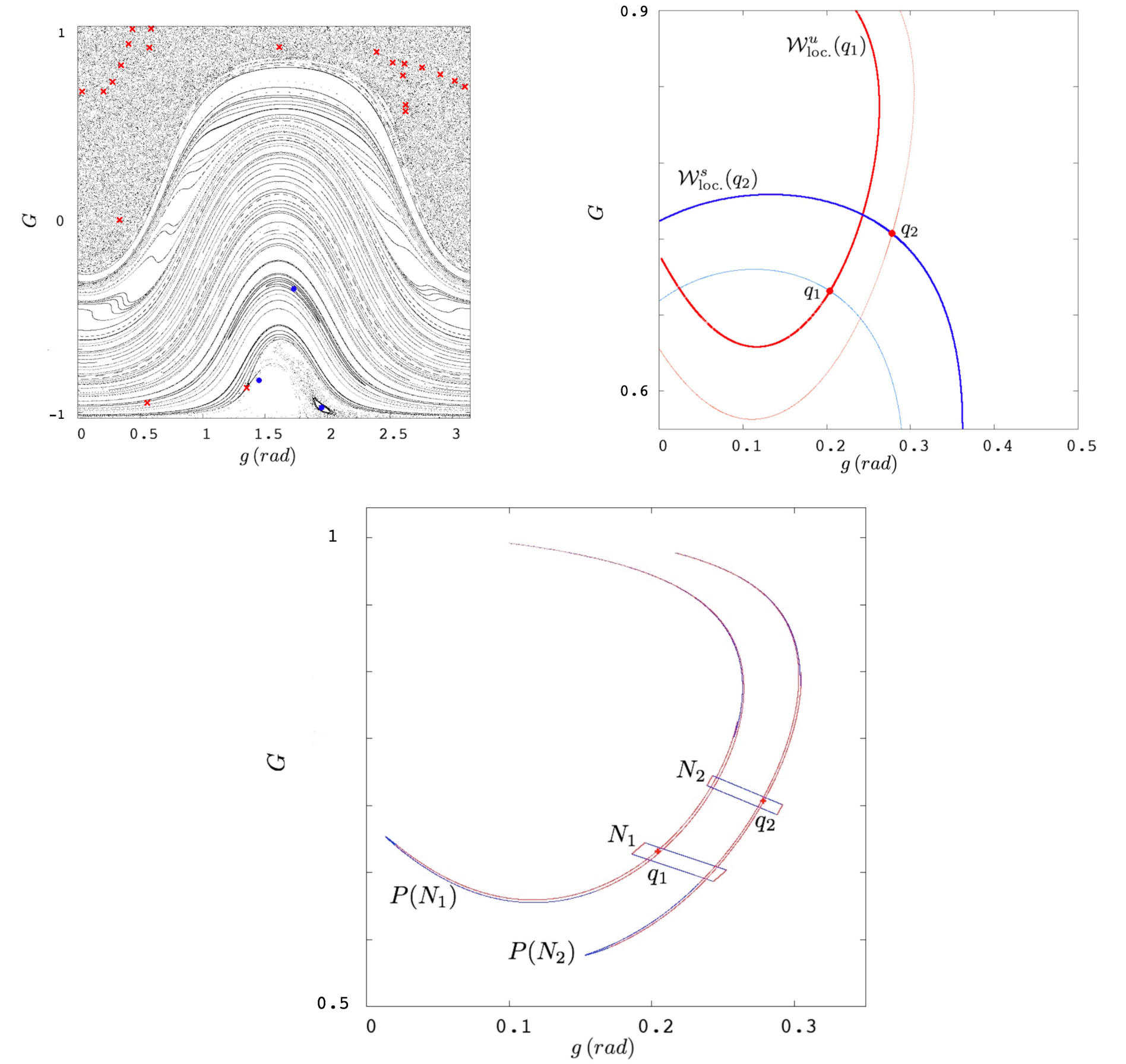
Figure 3: Composite panels illustrating our main steps in constructing the topological horseshoe. (Top left) The continuous flow is reduced to a 2–dimensional mapping by introducing a suitable Poincaré map $P$. The phase space contains both elliptic (blue) and hyperbolic (red) fixed-points. (Top right) Finite pieces of the stable and unstable manifolds might be constructed from the knowledge of the eigensystem derived from the linearisation $DP$. (Bottom) Carefully chosen sets and their images under $P$ provide the covering relations and imply existence of symbolic dynamics. See text for details.

Appendix A Outline of the proof of Theorem 3.1

In this section we provide some technical details of the proof of Theorem 3.1. For the full proof we refer to [18].

The proof is by recursion. We assume that, at a certain step, we have a system of the form

$${\rm H}({\mathbf{I}},\bm{{\varphi}},{\mathbf{J}}({\mathbf{p}},{\mathbf{q}}),y)={\rm h}({\mathbf{I}},{\mathbf{J}}({\mathbf{p}},{\mathbf{q}}),y)+g({\mathbf{I}},{\mathbf{J}}({\mathbf{p}},{\mathbf{q}}),y,x)+f({\mathbf{I}},\bm{{\varphi}},{\mathbf{J}}({\mathbf{p}},{\mathbf{q}}),y,x)$$ (141)

where $f\in{\cal O}_{{\rho},s,{\delta},r,\xi}$, $g\in{\cal N}_{{\rho},s,{\delta},r,\xi}$. At the first step, just take $g\equiv 0$.

After splitting $f$ on its Taylor–Fourier basis

$$f=\sum_{k,h,j}f_{khj}({\mathbf{I}},y,x)e^{{\rm i}k\cdot\bm{{\varphi}}}{\mathbf{p}}^{h}{\mathbf{q}}^{j}\,.$$

one looks for a time–1 map

$$\Phi=e^{{\cal L}_{\phi}}=\sum_{k=0}^{\infty}\frac{{\cal L}_{\phi}^{k}}{k!}\qquad{\cal L}_{\phi}(f):=\big{\{}\phi,\ f\big{\}}$$

generated by a small Hamiltonian $\phi$ which will be taken in the class ${\cal Z}_{{\rho},s,{\delta},r,\xi}$ in (97). Here,

$$\big{\{}\phi,\ f\big{\}} := \sum_{i=1}^{n}(\partial_{{\mathbf{I}}_{i}}\phi\partial_{\bm{{\varphi}}_{i}}f-\partial_{{\mathbf{I}}_{i}}f\partial_{\bm{{\varphi}}_{i}}\phi)+\sum_{i=1}^{m}(\partial_{{\mathbf{p}}_{i}}\phi\partial_{\mathbf{q}_{i}}f-\partial_{{\mathbf{p}}_{i}}f\partial_{\mathbf{q}_{i}}\phi)$$

$$+(\partial_{y}\phi\partial_{x}f-\partial_{y}f\partial_{x}\phi)$$

denotes the Poisson parentheses of $\phi$ and $f$. One lets

$$\phi=\sum_{(k,h,j):\atop{(k,h-j)\neq(0,0)}}\phi_{khj}({\mathbf{I}},y,x)e^{{\rm i}k\cdot\bm{{\varphi}}}{\mathbf{p}}^{h}{\mathbf{q}}^{j}\,.$$ (142)

The operation

$$\phi\to\{\phi,{\rm h}\}$$

acts diagonally on the monomials in the expansion (142), carrying

$$\phi_{khj}\to-\big{(}{\omega}_{y}\partial_{x}\phi_{khj}+{\lambda}_{khj}\phi_{khj}\big{)}\,,\quad{\rm with}\quad{\lambda}_{khj}:=(h-j)\cdot{\omega}_{\mathbf{J}}+{\rm i}k\cdot{\omega}_{\mathbf{I}}\,.$$ (143)

Therefore, one defines

$$\{\phi,{\rm h}\}=:-D_{\omega}\phi\,.$$

The formal application of $\Phi=e^{{\cal L}_{\phi}}$ yields:

$$e^{{\cal L}_{\phi}}{\rm H} = e^{{\cal L}_{\phi}}({\rm h}+g+f)={\rm h}+g-D_{\omega}\phi+f+\Phi_{2}({\rm h})+\Phi_{1}(g)+\Phi_{1}(f)$$ (144)

where the $\Phi_{h}:=\Phi_{h}:=\sum_{j\geq h}\frac{{\cal L}_{\phi}^{j}}{j!}$’s are the tails of $e^{{\cal L}_{\phi}}$.

Next, one requires that the residual term $-D_{\omega}\phi+f$ lies in the class ${\cal N}_{{\rho},s,{\delta},r,\xi}$ in (98)

$${(-D_{\omega}\phi+f)}\in{\cal N}_{{\rho},s,{\delta},r,\xi}$$ (145)

for $\phi$.

Since we have chosen $\phi\in{\cal Z}_{{\rho},s,{\delta},r,\xi}$, by (143), we have that also $D_{\omega}\phi\in{\cal Z}_{{\rho},s,{\delta},r,\xi}$. So, Equation (145) becomes

$$-D_{\omega}\phi+\mathaccent 869{f}=0\,.$$

In terms of the Taylor–Fourier modes, the equation becomes

$${\omega}_{y}\partial_{x}\phi_{khj}+{\lambda}_{khj}\phi_{khj}=f_{khj}\qquad\forall\ (k,h,j):\ (k,h-j)\neq(0,0)\,.$$ (146)

In the standard situation, one typically proceeds to solve such equation via Fourier series:

$$f_{khj}({\mathbf{I}},y,x)=\sum_{\ell}f_{khj\ell}({\mathbf{I}},y)e^{{\rm i}\ell x}\,,\qquad\phi_{khj}({\mathbf{I}},y,x)=\sum_{\ell}\phi_{khj\ell}({\mathbf{I}},y)e^{{\rm i}\ell x}$$

so as to find $\displaystyle\phi_{khj\ell}=\frac{f_{khj\ell}}{{\mu}_{khj\ell}}$ with the usual denominators ${\mu}_{khj\ell}:={\lambda}_{khj}+{\rm i}\ell\omega_{y}$ which one requires not to vanish via, e.g., a “diophantine inequality” to be held for all $(k,h,j,\ell)$ with $(k,h-j)\neq(0,0)$. In this standard case, there is not much freedom in the choice of $\phi$. In fact, such solution is determined up to solutions of the homogenous equation

$$D_{\omega}\phi_{0}=0$$ (147)

which, in view of the Diophantine condition, has the only trivial solution $\phi_{0}\equiv 0$. The situation is different if $f$ is not periodic in $x$, or $\phi$ is not needed so. In such a case, it is possible to find a solution of (146), corresponding to a non–trivial solution of (147), where small divisors do not appear. This is

$$\phi_{khj}({\mathbf{I}},y,x)=\left\{\begin{array}[]{l}\displaystyle\frac{1}{{\omega}_{y}}\int_{0}^{x}f_{khj}({\mathbf{I}},y,{\tau})e^{\frac{{\lambda}_{khj}}{{\omega}_{y}}({\tau}-x)}d{\tau}\quad{\rm if}\ \ (k,h-j)\neq(0,0)\\ \\ \displaystyle 0\qquad\qquad\qquad\qquad\qquad\qquad\qquad\ {\rm otherwise.}\end{array}\right.$$ (151)

Multiplying by $e^{ik{\varphi}}$ and summing over $k$, $h$ and $j$, we obtain

$$\phi({\mathbf{I}},{\bm{{\varphi}}},p,q,y,x)=\frac{1}{{\omega}_{y}}\int_{0}^{x}\mathaccent 869{f}\left({\mathbf{I}},{\bm{{\varphi}}}+\frac{{\omega}_{\mathbf{I}}}{{\omega}_{y}}({\tau}-x),pe^{\frac{{\omega}_{\mathbf{J}}}{{\omega}_{y}}({\tau}-x)},qe^{-\frac{{\omega}_{\mathbf{J}}}{{\omega}_{y}}({\tau}-x)},y,{\tau}\right)d{\tau}\,.$$

In [18] it is proved that, under the assumptions (3.1), this function can be used to obtain a convergent time–one map and that the construction can be iterated so as to provide the proof of Theorem 3.1. The construction of the iterations and the proof of its convergence is obtained adapting the techniques of  [19] to the present case.

Acknowledgments

The authors acknowledge the European Research Council (Grant 677793 Stable and Chaotic Motions in the Planetary Problem) for supporting them during the completion of the results described in the paper; warmly thank the organisers of I–CELMECH Training School that held in Milan in winter 2020 for their interest and especially U. Locatelli for a highlighting discussion.

References

- [1] V. I. Arnold. Mathematical Methods of Classical Mechanics, volume 60 of Graduate Texts in Mathematics. Springer-Verlag, New York, second edition (1989). Translated from the Russian by K. Vogtmann and A. Weinstein.
- [2] V. I. Arnold, V. V. Kozlov, and A. I. Neishtadt. Mathematical aspects of classical and celestial mechanics, volume 3 of Encyclopaedia of Mathematical Sciences. Springer-Verlag, Berlin, third edition (2006). [Dynamical systems. III], Translated from the Russian original by E. Khukhro.
- [3] A. A. Bekov and T. B. Omarov. Integrable cases of the Hamilton-Jacobi equation and some nonsteady problems of celestial mechanics. Soviet Astronomy, 22:366–370 (1978).
- [4] L. Chierchia and G. Pinzari. The planetary -body problem: symplectic foliation, reductions and invariant tori. Invent. Math., 186(1):1–77 (2011).
- [5] S. Di Ruzza, J. Daquin, and G. Pinzari. Symbolic dynamics in a binary asteroid system. Commun. Nonlinear Sci. Numer. Simul., 91:105414, 16 (2020).
- [6] H. R. Dullin and R. Montgomery. Syzygies in the two center problem. Nonlinearity, 29(4):1212–1237 (2016).
- [7] J. Féjoz. Démonstration du ‘théorème d’Arnold’ sur la stabilité du système planétaire (d’après Herman). Ergodic Theory Dynam. Systems, 24(5):1521–1582 (2004).
- [8] J. Féjoz and M. Guardia. Secular instability in the three-body problem. Archive for Rational Mechanics and Analysis, 221(1):335–362 (2016).
- [9] A. Gierzkiewicz and P. Zgliczyński. A computer-assisted proof of symbolic dynamics in hyperion’s rotation. Celestial Mechanics and Dynamical Astronomy, 131(7):33 (2019).
- [10] A. Giorgilli. Appunti di Meccanica Celeste. 2008. http://www.mat.unimi.it/users/antonio/meccel/Meccel˙5.pdf
- [11] A. Giorgilli, U. Locatelli, and M. Sansottera. Secular dynamics of a planar model of the sun-jupiter-saturn-uranus system; effective stability in the light of Kolmogorov and Nekhoroshev theories. Regular and Chaotic Dynamics, 22(1):54–77 (2017).
- [12] M. Guzzo and E. Lega. Evolution of the tangent vectors and localization of the stable and unstable manifolds of hyperbolic orbits by Fast Lyapunov Indicators. SIAM Journal on Applied Mathematics, 74(4):1058–1086 (2014).
- [13] C. G. J. Jacobi. Jacobi’s lectures on dynamics, volume 51 of Texts and Readings in Mathematics. Hindustan Book Agency, New Delhi, revised edition (2009). Delivered at the University of Königsberg in the winter semester 1842–1843 and according to the notes prepared by C. W. Brockardt, Edited by A. Clebsch, Translated from the original German by K. Balagangadharan, Translation edited by Biswarup Banerjee.
- [14] J. Laskar and P. Robutel. Stability of the planetary three-body problem. I. Expansion of the planetary Hamiltonian. Celestial Mech. Dynam. Astronom., 62(3):193–217 (1995).
- [15] G. Pinzari. On the Kolmogorov set for many–body problems. PhD thesis, Università Roma Tre, (2009).
- [16] G. Pinzari. A first integral to the partially averaged newtonian potential of the three-body problem. Celestial Mechanics and Dynamical Astronomy, 131(5):22 (2019).
- [17] G. Pinzari. Euler integral and perihelion librations. Discrete Continuous Dynamical Systems, (2020) 40(12):6919–6943.
- [18] G. Pinzari. Perihelion librations in the secular three-body problem. J. Nonlinear Sci., 30(4):1771–1808 (2020).
- [19] J. Pöschel. Nekhoroshev estimates for quasi-convex Hamiltonian systems. Math. Z., 213(2):187–216 (1993).
- [20] P. Zgliczynski and M. Gidea. Covering relations for multidimensional dynamical systems. Journal of Differential Equations, 202(1):32–58 (2004).