Physical properties of accretion shocks toward the Class I protostellar system Oph-IRS 44

Abstract

Context. The final outcome and chemical composition of a planetary system depend on its formation history: the physical processes that were involved and the molecular species available at different stages. Physical processes such as accretion shocks are thought to be common in the protostellar phase, where the envelope component is still present, and they can release molecules from the dust to the gas phase, altering the original chemical composition of the disk. Consequently, the study of accretion shocks is essential for a better understanding of the physical processes at disk scales and their chemical output.

Aims. The purpose of this work is to assess how the material from the infalling envelope feeds the disk and the chemical consequences thereof, particularly the characteristics of accretion shocks traced by sulfur-related species.

Methods. We present high angular resolution observations (0.1”, corresponding to 14 au) with the Atacama Large Millimeter/submillimeter Array (ALMA) of the Class I protostar Oph-IRS 44 (also known as YLW 16A). The continuum emission at 0.87 mm is observed, together with sulfur-related species such as SO, SO₂, and ³⁴SO₂. The non-local thermodynamic equilibrium (non-LTE) radiative-transfer tool RADEX and the rotational diagram method are employed to assess the physical conditions of the SO₂ emitting region.

Results. Six lines of SO₂, two lines of ³⁴SO₂, and one line of SO are detected toward IRS 44. The emission of all the detected lines peaks at $\sim$0.1” ($\sim$14 au) from the continuum peak and we find infalling-rotating motions inside 30 au. However, only redshifted emission is seen between 50 and 30 au. Colder and more quiescent material is seen toward an offset region located at a distance of $\sim$400 au from the protostar, and we do not find evidence of a Keplerian profile in these data. The SO₂ emitting region around the protostar is consistent with dense gas ($\geq$ 10⁸ cm^-3), temperatures above 70 K, high SO₂ column densities between 0.4 and 1.8 $\times$ 10¹⁷ cm^-2, line widths between 12 and 14 km s^-1, and an abundance ratio SO₂/SO $\geq$ 1, suggesting that some physical mechanism is enhancing the gas-phase SO₂ abundance.

Conclusions. Accretion shocks are the most plausible explanation for the high temperatures, high densities, and velocities found for the SO₂ emission. The offset region seems to be part of a localized streamer that is injecting material to the disk–envelope system through a protrusion observed only in redshifted emission and associated with the highest kinetic temperature. When material enters the disk–envelope system, it generates accretion shocks that increase the dust temperature and desorb SO₂ molecules from dust grains. High-energy SO₂ transitions (E_up $\sim$ 200 K) seem to be the best tracers of accretion shocks that can be followed up by future higher angular resolution ALMA observations and compared to other species to assess their importance in releasing molecules from the dust to the gas phase.

1 Introduction

The formation and evolution of protoplanetary disks are fundamental in the process of low-mass star formation, such as the formation of our own Solar System. A typical low-mass star forms when a molecular cloud with angular momentum collapses, and a protostar is formed at the central part with an infalling-rotating envelope whose inner part evolves to a circumstellar disk (Terebey et al. 1984; Shu et al. 1993; Hartmann 1998). Eventually, the star reaches its final mass, the envelope dissipates, and planets form in the disk. As a consequence, the final composition of planets is strongly dependent on the physical and chemical processes within the circumstellar disk. However, as disks first arise in the early stages of young stars (Jørgensen et al. 2009; Harsono et al. 2014; Yen et al. 2015) and the first steps of planet formation may occur when they are still deeply embedded (e.g., Harsono et al. 2018; Tychoniec et al. 2020), the chemical evolution of the material as it is accreted from the infalling envelope may play a key role.

The process of low-mass star formation comprises different stages (Robitaille et al. 2006), and Class I sources link the deeply embedded Class 0 sources (where the envelope is the dominant mass component) with the emergence of Class II disks (Keplerian disks with a negligible envelope). Class I sources are therefore the perfect candidates to study the connection between the envelope and the disk and, additionally, to investigate the dynamics and chemical composition of the young disk.

Theoretical models predict that the material from the envelope falls on the circumstellar disk and produces accretion shocks at the envelope–disk interface (Stahler et al. 1994; Yorke & Bodenheimer 1999; Krasnopolsky & Königl 2002). These accretion shocks have been invoked to explain the observed jump in density and drastic enhancement of SO toward the Class 0 and I sources L1527 and TMC-1A (Sakai et al. 2014, 2016), the asymmetric accretion found toward TMC-1A (Hanawa et al. 2022), and the emission of SO and SO₂ at the edge of the disks from two Class I/II sources, DG Tau and HL Tau (Garufi et al. 2022). Accretion shocks in dense ($\geq$ 10⁸ cm^-3) gas induce an increase in the dust temperature, and species that are locked in grain mantles are subsequently released into the gas phase, which affects the chemical content of the early disk (van Gelder et al. 2021). Although the presence of accretion shocks explains the jump in abundances observed for shock-related species and is the most plausible mechanism deduced from numerical simulations (Miura et al. 2017), only a few low-mass protostars show evidence of accretion shocks to date (e.g., Lee et al. 2014; Sakai et al. 2014; Garufi et al. 2022), and their physical parameters are not well constrained observationally. Apart from accretion shocks, contributions from disk winds or outflows would also be important (e.g., Bjerkeli et al. 2016; Alves et al. 2017; Tabone et al. 2017; Harsono et al. 2021). Therefore, observations at disk scales ($\sim$100 au) need to be performed to confirm the existence of accretion shocks, understand the origin of the observed abundances, and assess the physical parameters associated with this mechanism.

A suitable source for proving the nature of accretion shocks is Oph-IRS 44, a Class I source located in the Ophiuchus molecular cloud at a distance of 139 pc (average value for the L1688 cloud; Cánovas et al. 2019). Artur de la Villarmois et al. (2019) detected strong SO₂ emission toward a compact region ($\leq$ 60 au) in IRS 44, with an angular resolution of 0$\aas@@fstack{\prime\prime}$4 ($\sim$60 au). This particular SO₂ transition (18_4,14 – 18_3,15) is associated with an upper-level energy (E_up) of $\sim$200 K and its line profile shows a velocity range of $\sim$20 km s^-1. The angular resolution of 0$\aas@@fstack{\prime\prime}$4 of the data was not high enough to resolve the SO₂ emission and provide strong conclusions for the possible origin scenarios: accretions shocks, disk winds, or outflows.

IRS 44 was first identified as YLW 16A by Young et al. (1986) through IRAS observations, and other common names are Oph-emb 13, ISO-Oph 143, LFAM 35, and [GY92] 269, among others. It is associated with a bolometric temperature (T_bol) of 280 K, a bolometric luminosity (L_bol) of 7.1 L_⊙ (Evans et al. 2009), and an envelope mass (M_env) of 0.051 M_⊙ (for a distance of 139 pc; Jørgensen et al. 2009). IRS 44 has been proposed to be a protobinary system with a separation of $\sim$0$\aas@@fstack{\prime\prime}$3, based on observations with the Hubble Space Telescope (HST; Allen et al. 2002), the Very Large Telescope (VLT; Duchêne et al. 2007), and the Spitzer Space Telescope (McClure et al. 2010). Nevertheless, there is no evidence of a binary component in the submillimeter regime, through ALMA band 6 and band 7 observations (Sadavoy et al. 2019; Artur de la Villarmois et al. 2019).

In this paper we present high angular resolution 0$\aas@@fstack{\prime\prime}$1 (14 au) ALMA observations of multiple SO₂ molecular lines toward IRS 44. We discuss their potential to trace accretions shocks, and provide values of the physical parameters for the emitting gas. Section 2 describes the observational procedure, calibration, and the parameters of the observed molecular transitions. The observational results are presented in Sect. 3, while Sect. 4 is dedicated to the analysis of the data, with position-velocity diagrams, radiative-transfer models, estimations of rotational and excitation temperatures, and calculations of molecular column densities. We discuss the structure and kinematics of IRS 44 in Sect. 5, and end with a summary in Sect. 6.

2 Observations

IRS 44 was observed with ALMA during 2021 May 17 and 18 as part of the program 2019.1.00362.S (PI: Elizabeth Artur de la Villarmois). At the time of the observations, 47 and 45 antennas were available, respectively, in the array providing baselines between 15 and 2517 m. The observations targeted nine different spectral windows to observe multiple SO₂ lines, the less abundant ³⁴SO₂ isotopolog, and SO. The observed molecular transitions and their spectroscopic data are summarized in Table 1.

The calibration and imaging were done in CASA version 6.1.1 (McMullin et al. 2007). Gain and bandpass calibrations were performed through the observation of the quasars J1517–2422 and J1700–2610. Imaging was performed using the tclean task in CASA, where the Briggs weighting with a robust parameter of 0.5 was employed. The automasking option was chosen and the channel resolution is 0.21 km s^-1. The resulting dataset has a beam size of 0$\aas@@fstack{\prime\prime}$13 $\times$ 0$\aas@@fstack{\prime\prime}$09 (18 $\times$ 13 au) with a position angle (PA; measured from north to east) of -81$\degr$ and a largest angular scale (LAS) of 2$\aas@@fstack{\prime\prime}$3. The continuum rms level is 0.08 mJy beam^-1 and the rms level of each spectral window is listed in Table 1.

Table 1: Spectral setup and parameters of the observed molecular transitions.

Species	Transition	Frequency	Eup	Aij	rms (a)
		[GHz]	[K]	[$\times$10-5 s-1]	[mJy beam-1
					per channel]
SO	1011 – 1010	336.5538	143	1	2.8
SO2	167,9 – 176,12	336.6696	245	6	2.8
SO2	184,14 – 183,15	338.3060	197	33	2.4
SO2	201,19 – 192,18	338.6118	199	29	2.5
SO2	242,22 – 233,21	348.3878	293	19	2.7
SO2	53,3 – 42,2	351.2572	36	34	3.4
SO2	106,4 – 115,7	350.8628	139	4	3.2
34SO2	144,10 – 143,11	338.7857	134	31	2.5
34SO2	194,16 – 193,17	348.1175	213	35	2.8
34SO2(b)	96,4 – 105,5	351.0896	127	4	2.8

3 Results

3.1 Continuum emission

The continuum emission is shown in Fig. 1, where the horizontal component is slightly more extended than the vertical component, and the emission above 5$\sigma$ is contained within a radius of 0$\aas@@fstack{\prime\prime}$2 ($\sim$30 au). Two-dimensional (2D) Gaussians are used to fit emission in the image plane, obtaining an integrated flux of 22.9 $\pm$ 1.0 mJy, a peak flux of 16.91 $\pm$ 0.48 mJy beam^-1, and a deconvolved size of (0$\aas@@fstack{\prime\prime}$07 $\pm$ 0$\aas@@fstack{\prime\prime}$01) $\times$ (0$\aas@@fstack{\prime\prime}$06 $\pm$ 0$\aas@@fstack{\prime\prime}$01) with a PA of 119 $\pm$ 74$\degr$ (see the magenta ellipse in Fig. 1). The continuum peak position corresponds to $\alpha$ = 16^h27^m27^s.9858 $\pm$ 0^s.0002 and $\delta$ = -24$\degr$39$\arcmin$34$\aas@@fstack{\prime\prime}$063 $\pm$ 0$\aas@@fstack{\prime\prime}$001.

The disk mass at 0.87 mm was calculated from the continuum flux (22.9 $\pm$ 1.0 mJy) and using Eq. (2) from Artur de la Villarmois et al. (2018), which assumed optically thin emission, an opacity of 0.0175 cm^-2 per gram of gas at 0.87 mm, and a dust temperature of 30 K. A total mass M_gas+dust of (4.0 $\pm$ 0.2) $\times$ 10^-3 M_⊙ was obtained, adopting a dust temperature (T_dust) of 15 K, the value proposed by Dunham et al. (2014) for Class I sources. If T_dust = 30 K is assumed, the total mass decreases by a factor of $\sim$3. Given that the dust emission at 0.87 mm could be optically thick toward a Class I source, the calculated M_gas+dust represents a lower limit for the total mass.

Allen et al. (2002) and Duchêne et al. (2007) suggested that IRS 44 is a protobinary system with a separation of $\sim$0$\aas@@fstack{\prime\prime}$3. However, the continuum emission at 0.87 mm shows no binary detection in our ALMA data and we can only set an upper limit of 7 $\times$ 10^-5 M_⊙ for the total mass of a possible binary component (for a value of 5$\sigma$ and adopting the same parameters as in the previous paragraph).

Figure 1: Continuum emission (0.87 mm) toward IRS 44 above 5$\sigma$ ($\sigma$ = 0.08 mJy beam^-1). The white contours represent the weakest emission of [5$\sigma$, 10$\sigma$, 15$\sigma$, 20$\sigma$, and 25$\sigma$] for clarity. The black star shows the position of the continuum peak and the synthesized beam is indicated by the white filled ellipse. The magenta ellipse represents the deconvolved size from the 2D Gaussian fit.

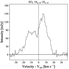
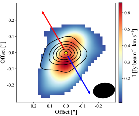
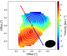
Figure 2: Emission of the SO₂ 18_4,14 – 18_3,15 line. Left: Spectrum rebinned by a factor of 4, integrated over a circular region with r = 0$\aas@@fstack{\prime\prime}$2, and centered on the continuum peak position. Center: Moment 0 map above 3$\sigma$ (color scale), integrated over 60 km s^-1, and continuum emission (black contours), starting at 20$\sigma$ and following steps of 40$\sigma$. Right: Moment 1 map (color scale) and moment 0 map (white contours) above 3$\sigma$. The blue and red arrows show the direction of the outflow from van der Marel et al. (2013), the yellow star indicates the continuum peak position, and the synthesized beam is represented by the black filled ellipse in the bottom right corner. The adopted systemic velocity is 3.7 km s^-1.

3.2 Molecular transitions

All the targeted molecular lines listed in Table 1 were detected toward IRS 44, with the exception of the ³⁴SO₂ 9_6,4 – 10_5,5 line. This nondetection is consistent with the low Einstein A coefficient (A_ij = 4 $\times$ 10^-5 s^-1) of the transition and it being a less abundant isotopolog. The six detected SO₂ lines have different upper level energies E_up, covering a broad range from 36 to 293 K. The brightest emission toward the continuum peak is from the SO₂ 18_4,14 – 18_3,15 line with E_up = 197 K, while there is an offset region located at a distance of $\sim$3$\aas@@fstack{\prime\prime}$0 ($\sim$400 au) from the protostar that shows bright emission of the SO₂ line related with the lowest energy: SO₂ 5_3,3 – 4_2,2 with E_up = 36 K.

Figure 2 presents the spectrum, and moment 0 and 1 maps of the SO₂ 18_4,14 – 18_3,15 line toward the central region. The spectrum was taken over a circular region with r = 0$\aas@@fstack{\prime\prime}$2 and shows a broad-line profile, from -20 to 20 km s^-1, and a decrease in the emission around the systemic velocity (V_sys) of 3.7 km s^-1, estimated from previous APEX observations (Lindberg et al. 2017). The moment 0 map reveals that the emission is concentrated around the protostar; however, the emission peak is slightly offset from the continuum peak, $\sim$0$\aas@@fstack{\prime\prime}$1 ($\sim$14 au), and corresponds to the redshifted component. The moment 1 map shows a clear rotational signature from northwest to southeast, with a PA of 157 $\pm$ 3$\degr$. The PA for the SO₂ 18_4,14 – 18_3,15 line emission was obtained from a 2D Gaussian fit of the moment 0 map. We note that this PA value is not perpendicular to the outflow direction (PA = 20$\degr$), which was estimated by van der Marel et al. (2013) using single-dish observations of CO 3-2. For the other detected lines (five SO₂, two ³⁴SO₂, and one SO line), the spectra and moment 0 and 1 maps are presented in the Appendix, in Figs. 10, 11, and 12, showing that SO₂, ³⁴SO₂, and SO exhibit a similar nature: broad spectra, emission concentrated around the protostar, and a clear rotational signature. In addition, all the detected transitions show that the peak of emission is offset south from the continuum peak position, at a distance of $\sim$0$\aas@@fstack{\prime\prime}$1 ($\sim$14 au). On average, the six SO₂ transitions show a full width at half maximum (FWHM) value of 12 km s^-1 for the blueshifted emission and 14 km s^-1 for the redshifted emission. Integrated fluxes of the observed transitions are presented in Table 2 in the Appendix.

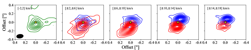
Figure 3: Contour maps of SO₂ 18_4,14 – 18_3,15 for different velocity ranges, shifted to 0 velocity. The contours start at 5$\sigma$ and follow steps of 5$\sigma$. The panel that includes the systemic velocity (3.7 km s^-1) is shown by the green contours in the first panel, while blue- and redshifted emission is represented by the blue and red contours, respectively. The yellow star shows the position of the source and the synthesized beam is indicated by the black filled ellipse in the bottom left corner of the first panel.

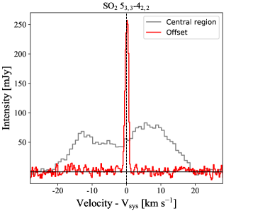
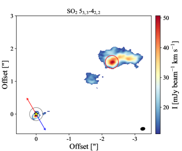
Figure 4: Emission of the SO₂ 5_3,3 – 4_2,2 line. Left: Spectra integrated over a circular region with r = 0$\aas@@fstack{\prime\prime}$2, centered on the continuum peak position (gray) and centered on the offset region (red). The spectrum taken at the continuum peak position has been rebinned by a factor of 4. Right: Moment 0 map above 3$\sigma$ integrated over 60 km s^-1. The gray and red circles represent the regions from which the spectra in the left panel were taken. The blue and red arrows show the direction of the outflow, the yellow star indicates the continuum peak position, and the synthesized beam is represented by the black filled ellipse in the bottom right corner. The adopted systemic velocity is 3.7 km s^-1.

Figure 3 shows contour maps of the SO₂ 18_4,14 – 18_3,15 line for different velocity ranges. Low-velocity contours (between -2 and 2 km s^-1) are concentrated around the protostar, but the weakest contours also present emission toward the west. Intermediate velocities, between $\pm$6 and $\pm$10 km s^-1, show that the redshifted emission is more extended than the blueshifted emission, possibly related with a protrusion from a localized streamer. Finally, a clear and symmetric rotating signature around the protostar is seen for high velocities ($\geq$10 km s^-1), which will be referred to as a disk–envelope structure.

At larger angular scales, the SO₂ 5_3,3 – 4_2,2 line (E_up = 36 K) shows bright emission toward an offset region, located at a distance of 2$\aas@@fstack{\prime\prime}$8 ($\sim$400 au) from the protostar, and its spectra and moment 0 map are presented in Fig. 4. The spectra were taken over the central region (gray) and the offset region (red), revealing that the offset region is associated with low velocities ($\leq$2 km s^-1), in contrast with the broad-line profile observed toward the central region, suggesting a different and more quiescent origin. Two other SO₂ lines (with E_up value of 197 and 199 K) show weaker emission toward the offset region and their moment 0 maps are presented in Fig. 13 in the Appendix. Given that the SO₂ line with the lowest E_up value (36 K) shows the brightest emission, the offset region is associated with colder gas, more consistent with a cloudlet or an SO₂ knot with a PA of 125 $\pm$ 7$\degr$. In this case the PA value was calculated by projecting a line that connects the continuum peak with the brightest pixel of the offset region, and it is consistent with the direction of the weakest contours seen in the first two panels of Fig. 3. The offset region is henceforth referred to as an SO₂ knot.

4 Analysis

4.1 Position–velocity diagrams

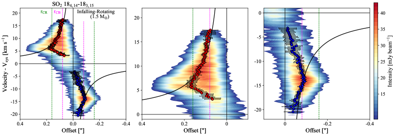
Figure 5: Position–velocity diagram for SO₂ 18_4,14–18_3,15. Left: Emission above 3$\sigma$, employing a PA of 157^∘. The blue and red dots represent blue- and redshifted emission peaks above $\pm$3 km s^-1, respectively. The black line represents an infalling-rotating profile with M_⋆ = 1.5M_⊙, an inclination of 70^∘, and r_CB = 0$\aas@@fstack{\prime\prime}$08 (magenta dashed lines). The r_CR is shown by the green dashed lies. Center: Zoomed-in version for the redshifted emission. Right: Zoomed-in version for the blueshifted emission. The systemic velocity is 3.7 km s^-1.

Figure 5 shows a position–velocity (PV) diagram for the SO₂ 18_4,14 – 18_3,15 line, employing a PA of 157$\degr$, with the peak emission of each channel superimposed. The peak emission was obtained through the CASA task imfit and the offset position was calculated by projecting the peak emission onto the disk position angle. The redshifted emission is more extended than the blueshifted emission: the former shows emission up to 0$\aas@@fstack{\prime\prime}$35 ($\sim$50 au) and the latter up to 0$\aas@@fstack{\prime\prime}$21 ($\sim$30 au). The central and right panels of Fig. 5 are zoomed-in versions of the red- and blueshifted emission. The high-velocity points are best fitted with an infalling-rotating profile (V_rot+inf), employing the equation

$$V_{\mathrm{rot+inf}}=\frac{\sqrt{2GM_{\star}sin(i)r_{CB}}}{r}\ ,$$ (1)

where G is the gravitational constant, M_⋆ the protostellar mass, r_CB the radius of the centrifugal barrier, i the inclination of the disk, and r the distance from the protostar. Equation 1 is from Oya et al. (2014), and the inclination term has been added explicitly. The r_CB is given by the maximum radial velocity (Sakai et al. 2014) and can be estimated from the PV diagram; the maximum radial velocity of 17.5 km s^-1 corresponds to r_CB =  0$\aas@@fstack{\prime\prime}$08 ($\sim$11 au). The maximum radial velocity changes depending on the assumption of V_sys; therefore, if V_sys changes by 0.5 km s^-1, r_CB will change by 0$\aas@@fstack{\prime\prime}$01 ($\sim$1.4 au). This leaves us with a degeneracy in the protostellar mass and the inclination, given by the term M_⋆sin(i). A protostellar mass of 1.5 M_⊙ is obtained if an inclination value of 70$\degr$ is assumed, following the interpretation of Terebey et al. (1992) that the outflow axis of IRS 44 lies close to the plane of the sky (from VLA observation of water masers). If we use other inclination values, such as 50$\degr$ and 90$\degr$, the points are well fitted with an infalling-rotating profile with a M_⋆ of 1.8 M_⊙ and 1.4 M_⊙, respectively. Seifried et al. (2016) proposed that the protostellar mass can be estimated by fitting the maximum velocity offset in the PV diagram (i.e., the borders above 3$\sigma$, which correspond to the outer envelope), instead of fitting the peak emission of each channel. Following this procedure, a protostellar mass of 4 M_⊙ is obtained.

The centrifugal barrier is the radius at which most of the gas kinetic energy contained in infalling motion is converted to rotational motion. The gas motion of the disk–envelope system outside r_CB can be regarded as infalling-rotating motion, while that inside can be regarded as Keplerian motion (Sakai et al. 2014; Oya et al. 2018). The r_CB is half of the centrifugal radius (r_CR), beyond which the gas is falling (Oya et al. 2018). From the SO₂ 18_4,14 – 18_3,15 line, r_CB = 0$\aas@@fstack{\prime\prime}$08 ($\sim$11 au) and r_CR = 0$\aas@@fstack{\prime\prime}$16 ($\sim$22 au). Beyond r_CR the more extended redshifted emission is seen, while no blueshifted counterpart is observed. This is consistent with the redshifted protrusion seen in the contour maps of Fig. 3 at velocities between 6 and 10 km s^-1, suggesting that a localized streamer might be infalling toward the system and, when entering the centrifugal radius at 0$\aas@@fstack{\prime\prime}$16, an infalling-rotating profile dominates the dynamics. A Keplerian disk is expected inside the centrifugal barrier of 0$\aas@@fstack{\prime\prime}$08; however, this is close to the resolution of our data and the presence of a Keplerian disk is not conclusive with the current data. If a Keplerian disk exists toward IRS 44, its radius will be $\leq$0$\aas@@fstack{\prime\prime}$08 ($\sim$11 au). Given that no Keplerian motions are observed in our data, the rotational signature seen in the moment 1 map of SO₂ (Fig. 2) suggests the presence of a disk–envelope structure and not a rotationally supported disk.

4.2 Column densities, kinetic temperatures, and optical depth

In this section we estimate kinetic temperatures (T_kin), SO₂ and SO molecular column densities (N${}_{\mathrm{SO_{2}}}$ and N_SO), and the optical depth of the lines by employing the non-LTE radiative transfer code RADEX (van der Tak et al. 2007). Later on, rotational temperatures (T_rot) and N${}_{\mathrm{SO_{2}}}$ of optically thin lines are estimated from the rotational diagram method, and excitation temperatures (T_ex) are assessed from optically thick lines.

4.2.1 Radiative transfer

The six different SO₂ transitions were employed to derive the gas density and temperature by comparing the observed relative intensities with those predicted by RADEX. The observed relative intensities are the quotient between the moment 0 maps, which present emission up to a radius of $\sim$0$\aas@@fstack{\prime\prime}$2. RADEX was run for a set of kinetic temperatures from 30 to 300 K, SO₂ column densities from 10¹² to 10¹⁸ cm^-2, and H₂ number density n_H between 10³ and 10⁹ cm^-3. Collisional rates for SO₂ were taken from the Leiden atomic and molecular database (LAMDA; Balança et al. 2016). A value of 5 km s^-1 was used for the broadening parameter (b), which corresponds to the line width observed in pixels far from the SO₂ peak. The brightest SO₂ line, which is associated with an E_up of 197 K, is used as a reference line.

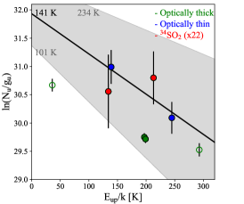
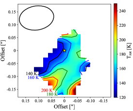
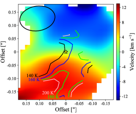
Figure 6: Temperature structure of IRS 44. Left: Rotational diagram at the source position, where only the optically thin SO₂ transitions (blue dots) and the ³⁴SO₂ lines (red dots) are used for the fit. The abundance ratio ³²S/³⁴S = 22 is from Wilson (1999). Optically thick SO₂ transitions (green dots) and those lines where the optical depth is not conclusive (open dots) show a significant offset with respect to the other lines, and they were not included in the calculation of the rotational temperature and SO₂ column densities. Center: Rotational temperature map created from optically thin SO₂ and ³⁴SO₂ transitions. Contours show specific values of 140, 160, 180, and 200 K. Right: Moment 1 map (right panel of Fig. 2) with the same specific values of the rotational temperature as those of the central panel, showing that the highest temperatures coincide with the redshifted protrusion. The synthesized beam is shown by the black ellipse in the upper left corner and the yellow star indicates the position of the source.

RADEX models with n_H between 10³ and 10⁷ cm^-3 were unable to explain the observed line ratios. The observed relative intensities are shown in Fig. 14, and they are compared with RADEX results for a H₂ number density of 10⁹ and 10⁸ cm^-3. The observed values provide a range of possibilities for T_kin and N${}_{\mathrm{SO_{2}}}$, given n_H. For n_H = 10⁸ cm^-3, there are no possible values that satisfy all the observed ranges, implying that the SO₂ emitting region is associated with n_H $\textgreater$ 10⁸ cm^-3. On the other hand, for n_H = 10⁹ cm^-3, T_kin should be higher than 90 K and 8 $\times$ 10¹⁶ $\leq$ N${}_{\mathrm{SO_{2}}}$ $\leq$ 8 $\times$ 10¹⁷ cm^-2. This possible values are shown in Fig. 15.

For n_H = 10⁹ cm^-3, the optical depth of the six SO₂ lines is analyzed, taking into account the possible values of T_kin and N${}_{\mathrm{SO_{2}}}$. Figure 16 shows that, from the six SO₂ lines, two are optically thick (SO₂ 18_4,14 – 18_3,15 and SO₂ 20_1,19 – 19_2,18), two are optically thin (SO₂ 16_7,9 – 17_6,12 and SO₂ 10_6,4 – 11_5,7), and nothing conclusive can be said about the remaining two (SO₂ 5_3,3 – 4_2,2 and SO₂ 24_2,22 – 23_3,21).

4.2.2 Rotational diagram

For optically thin SO₂ lines and the less abundant isotopolog ³⁴SO₂, the beam-averaged column densities and rotational temperatures can be assessed by the rotational diagram analysis, summarized by Goldsmith & Langer (1999). The gas is assumed to be under local thermodynamic equilibrium (LTE); therefore, all the molecular transitions can be characterized by a single excitation temperature, also called rotational temperature (T_rot). In this regime the following equation is valid:

$$\ln\frac{N_{\mathrm{u}}}{g_{\mathrm{u}}}=\frac{-1}{T_{\mathrm{rot}}}\frac{E_{\mathrm{u}}}{k}+\ln\frac{N}{Q(T_{\mathrm{rot}})}\ .$$ (2)

Here N_u is the column density of the upper level, g_u the level degeneracy, E_u/k the energy of the upper level in K, k the Boltzmann constant, N the total column density of the molecule, and Q(T_rot) the partition function that depends on the rotational temperature.

Under the optically thin condition, N_u is obtained from

$$N_{\mathrm{u}}=\frac{8\pi k\nu^{2}W}{hc^{3}A_{ul}}\ ,$$ (3)

where $\nu$ is the line frequency, W the integrated line intensity, c the speed of light, and A_ul the Einstein coefficient for spontaneous emission. Equation 3 can be rewritten as

$$N_{\mathrm{u}}=1943.59\ \left(\frac{\nu}{1\ \mathrm{GHz}}\right)^{2}\ \left(\frac{W}{1\ \mathrm{K\ km\ s^{-1}}}\right)\ \left(\frac{1\ \mathrm{s^{-1}}}{A_{\mathrm{ul}}}\right)\ ,$$ (4)

where N_u is obtained in units of cm^-2.

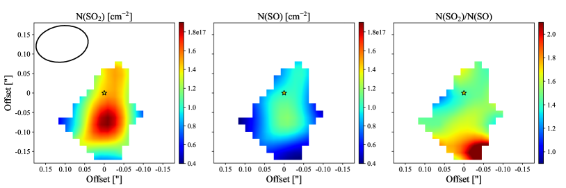
Figure 7: Column densities. Left: SO₂ column density obtained from the rotational diagram method. The synthesized beam is shown by the black ellipse in the upper left corner. Center: SO column density, assuming optically thin emission and employing the rotational temperatures from Fig. 6. Right: Column density ratio of SO₂ to SO. The yellow star indicates the position of the source.

Equations 2 and 4 were used to calculate T_rot and create the map shown in Fig. 6. For each pixel, only the optically thin SO₂ lines and ³⁴SO₂ isotopologs were used to fit the rotational temperature. For ³⁴SO₂, an abundance ratio ³²S/³⁴S = 22 (Wilson 1999) was adopted. The left panel of Fig. 6 shows the example of the fit from the pixel that corresponds to the source position and a clear offset is seen between optically thin (blue and red dots) and optically thick lines (green dots). The detection of optically thin lines and the less abundant isotopolog, ³⁴SO₂, is crucial for an accurate estimate of the rotational temperature, and consequently for the SO₂ column density as well. The T_rot map (central and right panels of Fig. 6) shows high temperatures ($\geq$120 K) in the region where the SO₂ emission arises. In addition, the warmest region, southeast from the protostar, seems to correlate with the redshifted protrusion. When infalling material reaches the surface layers of the disk–envelope structure, it generates accretion shocks that are predicted to increase the temperature and the density by up to two orders of magnitude ($\sim$10⁹ cm^-3; van Gelder et al. 2021). If the dust temperature exceeds 60 K, SO₂ molecules can efficiently desorb from dust grains.

Figure 7 shows the SO₂ and SO column densities, and the ratio between them. The region where the six SO₂ lines are detected shows N${}_{\mathrm{SO_{2}}}$ values between 1.0 and 1.8 $\times$ 10¹⁷ cm^-2, while N_SO presents lower values, between 0.6 and 1.3 $\times$ 10¹⁷ cm^-2. Since there is only one observed (and detected) SO line, RADEX was employed using the same temperature and density parameters as SO₂ (i.e., n_H = 10⁹ cm^-3 and T_kin = 90 K), concluding that this SO line in particular is optically thin. The column density ratio between SO₂ and SO is shown in the right panel of Fig. 7 and it is found to be higher than 1 toward the SO₂ emitting region.

4.2.3 Optically thick lines

As seen in Sect. 4.2.1, two out of six SO₂ lines are optically thick. For optically thick lines, the peak temperature (T_peak) provides a good measure of (T_ex) with

$$T_{\mathrm{ex}}=\frac{E_{\mathrm{up}}}{k}\left[\mathrm{log}\left(\frac{E_{\mathrm{up}}}{kT_{\mathrm{peak}}}+1\right)\right]^{-1}\ .$$ (5)

Equation 5 is from Goicoechea et al. (2016) and, if n_H is much higher than the critical density of the transition (n_crit), the line is close to thermalization and T_ex approaches T_gas. From the two optically thick SO₂ lines, the line with the lowest n_crit ($\sim$10⁷ cm^-3) corresponds to SO₂ 18_4,14–18_3,15. This transition line was used to create the temperature map shown in Fig. 8, where T_peak was obtained from a moment 8 map (which provides the maximum value of the spectrum in each pixel). The southern region presents a more extended and elongated structure in the excitation temperature map, consistent with the redshifted protrusion (see also Figs. 2, 3, and 6), and T_ex $\geq$ 70 K are found for the SO₂ emitting region. Given that the $\tau$ value of this line lies between 1 and 7 (see first panel of Fig. 16), it may not be fully thermalized, and therefore the temperature map in Fig. 8 represents a lower limit for T_ex. These excitation temperatures are consistent with those found in Sect. 4.2.2 from the rotational diagram method using optically thin transitions.

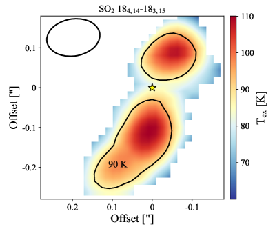
Figure 8: Excitation temperature of the optically thick SO₂ 18_4,14–18_3,15 transition using Eq. 5. The black contour represents the specific value of 90 K. The yellow star indicates the position of the source and the synthesized beam is shown by the black ellipse in the upper left corner.

5 Discussion

5.1 Accretion shocks, disk winds, or outflows?

The molecules SO and SO₂ are known as shock tracers and there are three main physical origins for these shocks: outflows (e.g., Tafalla et al. 2010; Persson et al. 2012), disk winds (e.g., Tabone et al. 2017), and accretion shocks (e.g., Sakai et al. 2014; Garufi et al. 2022).

For IRS 44 the outflow scenario can be ruled out from the shape of the PV diagram shown in Fig. 5 and the high densities ($\geq$10⁸ cm^-3) found for the SO₂ emitting region. PV diagrams related with outflow emission show that the velocity linearly increases as a function of the distance to the protostar (e.g., Lee et al. 2000; Arce et al. 2013) and densities below 10⁸ cm^-3 have been found in the inner regions of the outflow cavity associated with young protostars (Kristensen et al. 2013). In addition, the broadness of the SO₂ lines rules out the envelope origin, where typical line widths are below 2 km s^-1 (e.g., Harsono et al. 2021).

As disk winds are related with gas that is ejected at small radial distances from the central source (e.g., Bjerkeli et al. 2016; Alves et al. 2017), some degree of symmetry is expected on the surface layers of the disk, such as a butterfly shape. Tabone et al. (2017) have proposed that the SO and SO₂ emission detected toward the Class 0 source HH212 originates from a disk wind between $\sim$50 and $\sim$150 au. Nevertheless, Panoglou et al. (2012) have shown that species such as SO survive between 10 and 100 au in disk winds toward Class 0 sources, but they get destroyed by photodissociation beyond $\sim$1 au in disk winds from more evolved Class I sources. The SO₂ emission does not show the expected symmetry for a disk wind and the kinematic analysis indicates that the material follows an infalling-rotating profile without a Keplerian signature. If disk winds are present, we expect them to arise from the disk surface layers, likely inside 0$\aas@@fstack{\prime\prime}$08 (11 au).

The high temperatures estimated from optically thin ($\geq$120 K) and optically thick ($\geq$70 K) lines (Figs. 6 and 8), the moderate velocities (between 12 and 14 km s^-1), and the high densities ($\geq$ 10⁸ cm^-3) found for IRS 44 are in agreement with the accretion shock scenario. van Gelder et al. (2021) have shown that accretion shocks can efficiently desorb SO₂ from dust grains when moderate velocities ($\geq$ 10 km s^-1) and high densities ($\geq$ 10⁸ cm^-3) are present. For densities above 3 $\times$ 10⁴ cm^-3, the gas and the dust are efficiently coupled, T_dust = T_gas (Evans et al. 2001; Galli et al. 2002), and a dust temperature above 62 K is required in order to sublimate SO₂ molecules from dust grains (Penteado et al. 2017; van Gelder et al. 2021). In interstellar ices, SO₂ is tentatively detected (Boogert et al. 1997; Zasowski et al. 2009); however, chemical models predict that SO₂ is the most abundant species in the gas in the warm-up phase, when the protostar is formed (Woods et al. 2015).

Accretion shocks would also desorb SO molecules form dust grains and the gas-phase abundance of SO₂ could increase through the reaction of SO with OH (Charnley 1997; van Gelder et al. 2021). Nevertheless, Karska et al. (2018) did not detect OH toward IRS 44 from Herschel/PACS observations, suggesting that the gas-phase formation of SO₂ by oxidation of SO could be ruled out. SO₂/SO $\geq$ 1 also suggests that the radiation field from the protostar is not efficiently photo-dissociating SO₂ into SO (e.g., Booth et al. 2021) and that the cosmic ray ionization rate is low ($\zeta$= 1.3 $\times$ 10¹⁷ s^-1, Woods et al. 2015).

In this section we suggest that SO and SO₂ molecules toward IRS 44 sublimate from heated dust grains by the accretion shocks with moderate velocity shocks ($\geq$ 10 km s^-1) and high densities ($\geq$ 10⁸ cm^-3). If there is a chemical reaction that contributes to the SO₂ abundance in the gas phase, it should be a different one from the reaction of SO with OH. Future observations of other molecular species, such as OCS, H₂S, and H₂CO, will confirm the formation path of SO₂: direct desorption from dust grains, gas-phase formation, or a combination of both. H₂S and H₂CO are directly linked to the gas-phase formation of SO and SO₂, while OCS presents a similar desorption temperature to SO, but it does not participate in the gas-phase chemistry (Charnley 1997).

5.2 Morphology of IRS 44

Given that (i) quiescent and colder SO₂ emission is present at $\sim$2$\aas@@fstack{\prime\prime}$8, (ii) a redshifted protrusion is seen at velocities between 2 and 10 km s^-1, (iii) the highest temperatures seem to correlate with the redshifted protrusion, (iv) blueshifted material beyond 0$\aas@@fstack{\prime\prime}$2 ($\sim$30 au) is absent, and (v) the SO₂ emission peak is observed at a distance of $\sim$0$\aas@@fstack{\prime\prime}$1 from the continuum peak (at redshifted velocities), a localized streamer might be accreting material to the envelope–disk system and generating accretion shocks that release SO₂ molecules from the dust to the gas phase. Figure 9 shows a schematic representation of IRS 44 and the localized streamer, which would be located between the observer and the disk–envelope component and would feed the system toward the redshifted protrusion. As IRS 44 is classified as a Class I source, meaning that the envelope is still present but largely dissipated (M_env = 0.051 M_⊙ for a distance of 139 pc; Jørgensen et al. 2008, 2009), it is more likely that the infalling of material occurs through streamers and not in a spherically symmetric way. A similar behavior is seen toward the Class I source TMC-1A, as asymmetric CS and SO emission is explained by a cloudlet capture and subsequent formation of an infalling streamer (Hanawa et al. 2022), and the more evolved Class I/II sources DG Tau and HL Tau (Garufi et al. 2022), where accretion shocks traced by SO and SO₂ are located along the late infalling streamers still feeding the system.

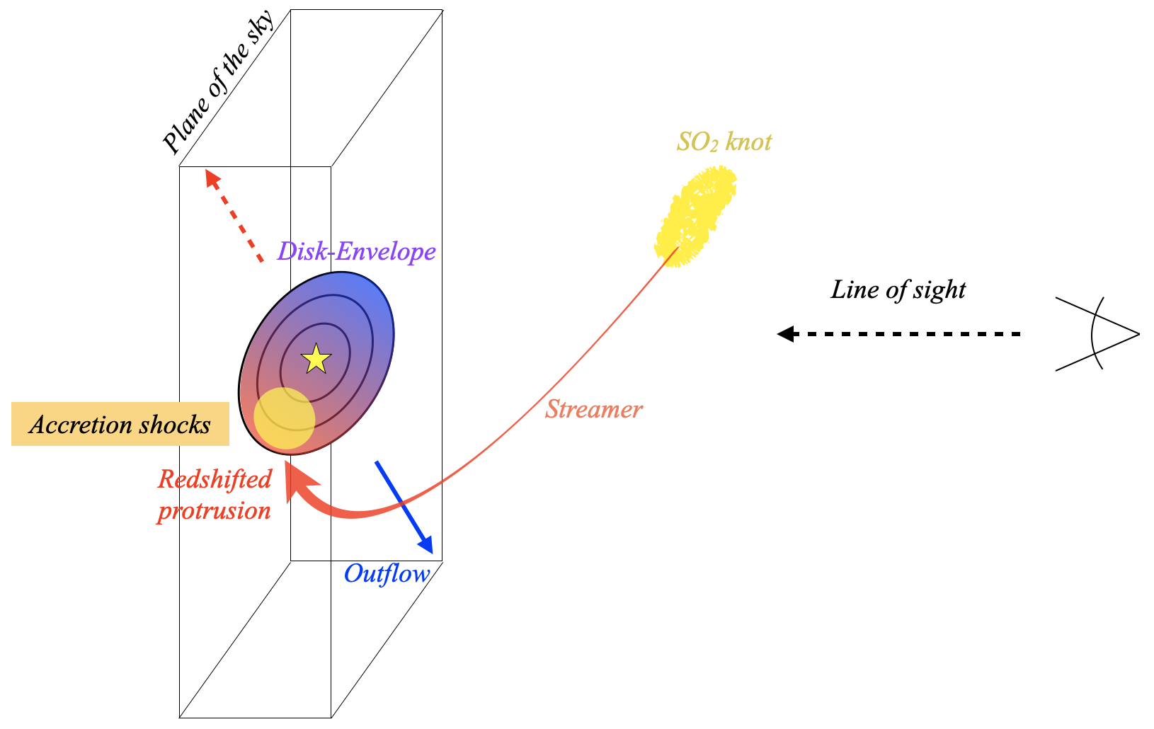
Figure 9: Schematic representation of IRS 44. The quiescent SO₂ emission (knot) would be part of a streamer that allows material to fall into the disk–envelope through the redshifted protrusion and generate accretion shocks. These shocks sublimate SO₂ molecules from dust grains and enhance the SO₂ gaseous abundance, showing an emission peak $\sim$0$\aas@@fstack{\prime\prime}$1 to the south of the protostar.

5.3 Outflow direction vs. disk–envelope direction

As seen in Fig. 2, the disk–envelope direction (157$\degr$) is not perpendicular to that of the single-dish outflow (20$\degr$). The latter is seen at large scales ($\sim$30$\arcsec$) and the outflow direction may vary due to the surrounding gas. If the misalignment is real, this could be due to the presence of a binary component, a cloudlet capture, or physical processes during the formation history, such as misalignment between the cloud rotation axis and the initial B-field direction, formation from a turbulent core, or non-ideal magnetohydrodynamics (MHD) effects.

Terebey et al. (2001) proposed that IRS 44 is a protobinary system with a separation of 0$\aas@@fstack{\prime\prime}$27 and PA = 81$\degr$, based on HST observations. The primary component has been detected at 1.60, 1.87, and 2.05 $\mu$m, while the secondary component is only visible at the longest wavelength, at 2.05 $\mu$m. Nevertheless, there is no sign of binarity toward IRS 44 in the submillimeter regime, following this work with an angular resolution of $\sim$0$\aas@@fstack{\prime\prime}$1 and the ALMA data presented in Artur de la Villarmois et al. (2019) and Sadavoy et al. (2019), which report an angular resolution of $\sim$0$\aas@@fstack{\prime\prime}$4 and $\sim$0$\aas@@fstack{\prime\prime}$25, respectively. The HST emission in 2.05 $\mu$m could therefore be associated with scattered light and not a binary component or the binary could be very faint at submillimeter wavelengths (below our sensitivity).

In the case of a cloudlet capture, each cloudlet should have a different angular momentum vector and the capture process can potentially change the rotation axis of the disk (e.g., Dullemond et al. 2019; Kuffmeier et al. 2020; Hanawa et al. 2022). The presence of a localized streamer toward IRS 44 could be affecting the rotation axis of the disk–envelope, and the result would depend on the mass and the angular momentum vector of the infalling material.

The misalignment between the cloud rotation axis and the initial B-field direction can create a warped disk structure during the protostellar core collapse (Hirano & Machida 2019), and B-fields in protostellar cores appear to be randomly aligned with their respective outflows (Hull et al. 2014; Lee et al. 2017). In the absence of a binary component, this initial misalignment could explain the change in direction observed toward IRS 44. A similar situation was proposed for the Class I disk L1489 (Sai et al. 2020), where the observation of a warped disk is explained by the initial misaligment between the initial B-field direction and the angular momentum vector.

Different velocity gradients between the direction of the rotationally supported disk and the direction of the envelope rotation were seen for a handful of Class 0/I sources (Brinch et al. 2007; Harsono et al. 2014). This misalignment might be due to formation from turbulent cores or non-ideal MHD effects, such as the Hall effect (e.g., Li et al. 2011; Braiding & Wardle 2012).

5.4 Nondetection of C¹⁷O and absence of warm CH₃OH toward IRS 44

Previous observations of IRS 44 do not detect C¹⁷O (3–2) and warm CH₃OH (E_up = 65 K) at an angular resolution of 0$\aas@@fstack{\prime\prime}$4 ($\sim$60 au); Artur de la Villarmois et al. 2019). C¹⁷O is commonly associated with Keplerian disks in Class I sources, and its nondetection might be related with the absence of a Keplerian disk, at least outside 11 au. CH₃OH, on the other hand, is hardly detected in Class I sources (Artur de la Villarmois et al. 2019); however, its gas-phase abundance is enhanced in shocked regions and a correlation between SO₂ and CH₃OH is expected. That SO₂ shows strong emission and CH₃OH is not detected toward IRS 44 might be related with one of the following possibilities: (i) CH₃OH is being desorbed form dust grains, but later on it is destroyed by the moderate velocities of the shocks ($\geq$10 km s^-1; Suutarinen et al. 2014); (ii) the formation of CH₃OH on the grain surfaces, from H₂CO, is not efficient; (iii) the presence of a disk results in colder gas (Lindberg et al. 2014; van Gelder et al. 2022); or (iv) optically thick dust can hide the emission of COMs (Nazari et al. 2022). Future observations of H₂CO could clarify the CH₃OH nondetection, and clearly there is some uncertainty regarding the origin of the SO₂ emission. The origin of this may be related to the uncertain carrier of elemental sulfur in protostellar envelopes. This carrier must be subject to destruction in shocks and clearly carry both S and O.

6 Summary

This work presents high angular resolution ($\sim$0$\aas@@fstack{\prime\prime}$1, 14 au) ALMA observations of the Class I source IRS 44. The continuum emission at 0.87 mm is analyzed, together with molecular species such as SO, SO₂, and ³⁴SO₂. The main results are summarized below:

• The continuum emission is contained within a radius of $\sim$0$\aas@@fstack{\prime\prime}$2 (30 au) and a total mass (gas + dust) of 4.0 $\times$ 10^-3 M_⊙ is calculated for IRS 44. Given that no binary component is detected with our sensitivity, an upper limit of 7 $\times$ 10^-5 M_⊙ is estimated for its total dust mass.

• One SO, six SO₂, and two out of three ³⁴SO₂ lines are detected; all of the detections show two components in their spectra, a blueshifted one and a redshifted one, both with broad linewidths (between -20 and 20 km s^-1). At small scales ($<$ 0$\aas@@fstack{\prime\prime}$3) the brightest SO₂ line is associated with high E_up = 197 K, while the SO₂ line with low E_up = 36 K presents the brightest emission at larger angular scales (between 2$\arcsec$ and 3$\arcsec$), shows narrow lines below 2 km s^-1, and has been associated with a shocked region.

• Around the protostar, SO₂ shows that the redshifted component is more extended than the blueshifted one, likely related with a redshifted protrusion, and the velocity profile is better fitted with an infalling-rotating profile with M_⋆ = 1.5 M_⊙ and r_CB = 0$\aas@@fstack{\prime\prime}$08. The quiescent shocked region and the redshifted protrusion seem to be part of a localized streamer, allowing material to fall to the disk–envelope and generate accretion shocks. No evidence of Keplerian motions are found; however, a Keplerian disk is expected inside r_CB.

• The comparison between observed relative intensities of the various lines and RADEX results indicates that the SO₂ emission around the protostar arises from a dense region (n_H $\geq$ 10⁸ cm^-3) with kinetic temperatures above 90 K. In addition, two SO₂ lines are clearly optically thin lines and two others are optically thick lines.

• The rotational diagram provides kinetic temperatures between 120 and 250 K for the SO₂ emitting region, where the warmest regions coincide with the location of the redshifted protrusion, and SO₂ column densities lie between 0.4 and 1.8 $\times$ 10¹⁷ cm^-2. SO column densities are a little lower, between 0.4 and 1.2 $\times$ 10¹⁷ cm^-2, and as a consequence the N(SO₂)/N(SO₂) ratio lies between 1.0 and 2.0.

• Optically thick SO₂ lines provide T_ex values between 70 and 110 K (regarded as lower limits) and a temperature structure consistent with warmer material arising from the south.

• The high temperatures, compact emission, high n_H densities, and moderate velocities agree with the accretion shock scenario, where molecules are being efficiently sublimated from dust grains. We can conclude, therefore, that accretion shocks toward IRS 44 are associated with n_H $\geq$ 10⁸ cm^-3, T_kin $\geq$ 90 K, T_rot between 120 and 240 K, T_ex $\geq$ 70 K, SO₂ column densities between 0.4 and 1.8 $\times$ 10¹⁷ cm^-2, and velocities between 12 and 14 km s^-1.

• Finally, high-energy SO₂ lines (E_up $\sim$ 200 K) seem to be the best tracers of accretion shocks

Accretion shocks might have important consequences for the chemical content of the disk and the release of neutral species, such as H₂O and COMs. It is therefore an important physical process that should be studied in more detail, and high angular resolution observations are essential for this purpose. Future observations of other Class I sources that show bright SO₂ emission will be necessary to increase the statistics and achieve a more complete picture of accretion shocks. Other molecular species such as CS, OCS, H₂S, and H₂CO could provide key additional information. CS is the most abundant sulfur-bearing species in young disks and OCS desorbs from dust grains at a similar temperature than SO, but it does not participate in the gas-phase chemistry below 300 K. H₂CO and H₂S are key species in the gas-phase formation of SO and SO₂. In addition, H₂CO is a good tracer of the gas temperature and it has similar desorption temperature to SO₂. Finally, a kinematic study of CO isotopologs, in special C¹⁸O, could provide information about the existence of a Keplerian disk.

Appendix A SO₂, ³⁴SO₂, and SO detections

The integrated fluxes of the detected transitions, and upper limits for nondetections, are presented in Table 2, where a region with r = 0$\aas@@fstack{\prime\prime}$2 and centered on the continuum peak position was chosen. The spectra, moment 0, and moment 1 maps of the detected transitions at small scales are shown in Figs. 10, 11, and 12, respectively. Figure 13 presents the large-scale emission, where only three SO₂ lines were detected.

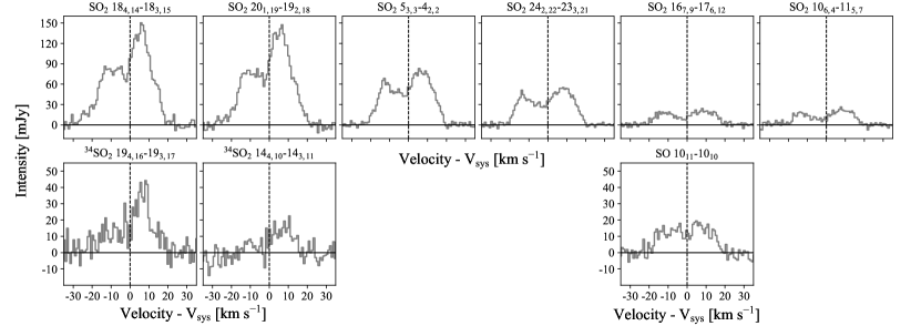
Figure 10: Spectra of SO₂ (top), ³⁴SO₂ (bottom left), and SO (bottom right), integrated over a circular region with r = 0$\aas@@fstack{\prime\prime}$2 and centered on the continuum peak position. The systemic velocity corresponds to 3.7 km s^-1.

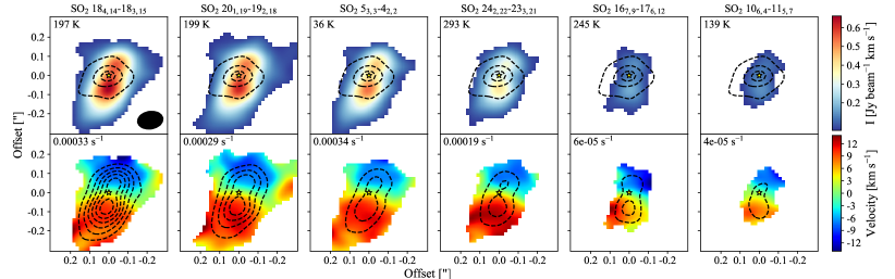
Figure 11: Small-scale emission. Top: Moment 0 maps of SO₂ above 3$\sigma$ (color scale) and continuum emission (dashed contours). The moment 0 maps were integrated over 60 km s^-1 and the continuum contours start at 20$\sigma$ and follow steps of 80$\sigma$. The E_up value of each transition is indicated in the top left corner of each panel and the synthesized beam is shown by the black filled ellipse in the bottom right corner of the first panel. The color scale is the same for the six panels. Bottom: Moment 1 maps of SO₂ above 3$\sigma$ (color scale) and selected values of their respective moment 0 maps (dashed contours). The contours start at 3$\sigma$ and follow steps of 7$\sigma$, with the exception of the last two panels, which follow steps of 3$\sigma$. The A_ij value of each transition is indicated in the top left corner of each panel; the color scale is the same for the six panels. The adopted systemic velocity is 3.7 km s^-1.

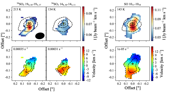
Figure 12: Same as Fig. 11, but for ³⁴SO₂ and SO. The dashed black contours in the moment 1 maps follow steps of 1$\sigma$ and 3$\sigma$ for ³⁴SO₂ and SO, respectively.

Table 2: Integrated fluxes over a velocity range of 60 km s^-1 and taking a circular region with r = 0$\aas@@fstack{\prime\prime}$2 centered on the continuum peak position.

Species	Transition	Flux density
		[mJy km s-1]
SO	1011 – 1010	624 $\pm$ 14
SO2	167,9 – 176,12	791 $\pm$ 17
SO2	184,14 – 183,15	2919 $\pm$ 18
SO2	201,19 – 192,18	2802 $\pm$ 17
SO2	242,22 – 233,21	1782 $\pm$ 19
SO2	53,3 – 42,2	2626 $\pm$ 23
SO2	106,4 – 115,7	700 $\pm$ 19
34SO2	144,10 – 143,11	221 $\pm$ 13
34SO2	194,16 – 193,17	547 $\pm$ 18
34SO2	96,4 – 105,5	$\leq$ 51 (a)

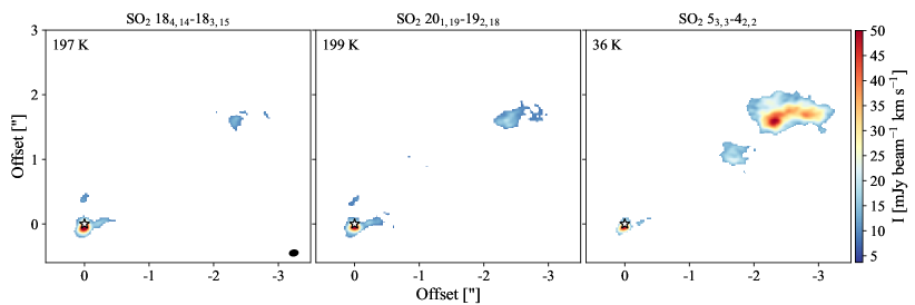
Figure 13: Large-scale emission. Moment 0 maps of SO₂ integrated over a velocity range of 2 km s^-1 and above 1$\sigma$. The white star shows the position of the source and the synthesized beam is indicated by the black filled ellipse in the bottom right corner of the first panel. The E_up value of each transition is indicated in the top left corner of each panel and the color scale is the same for all three panels.

Appendix B Radiative transfer

The six different SO₂ transitions were employed to compare the observed relative intensities with values obtained from RADEX. The observed relative intensities are shown in the upper row of Fig. 14. The middle and bottom rows show the RADEX results for a H₂ number density of 10⁹ and 10⁸ cm^-3, respectively, and the contour levels represent the observed values (shown in the top row). An error value of 1$\sigma$ (employing error propagation) was added to the observed ratios and is represented by the black dashed contours in the RADEX results.

For n_H = 10⁸ cm^-3 (bottom row of Fig. 14), the third panel (197/293) and the fifth panel (197/139) do not present an overlapping region; therefore, this density does not reproduce the observed values and n_H should be higher than 10⁸ cm^-3. On the other hand, for n_H = 10⁹ cm^-3 (middle row of Fig. 14), the possible ranges are presented in Fig. 15 and the possible values consist of T_kin $\geq$ 90 K and N${}_{\mathrm{SO_{2}}}$ between 8 $\times$ 10¹⁶ and 8 $\times$ 10¹⁷ cm^-2.

Figure 16 shows the optical depth of the six SO₂ transitions, obtained with RADEX with n_H = 10⁹ cm^-3, and the possible values discussed above are shown in gray dashed contours. The brightest transitions, those with E_up values of 197 and 199 K, are optically thick lines, while the two weakest ones (E_up of 245 and 139 K) are optically thin lines. Nothing conclusive can be said for those transitions with E_up values of 36 and 293 K.

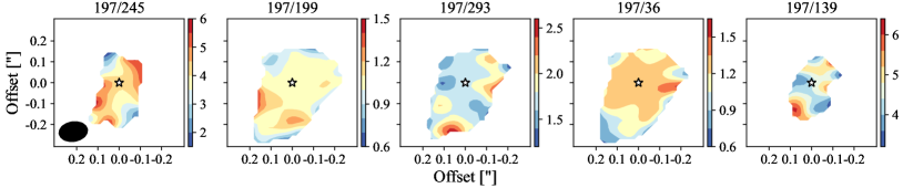
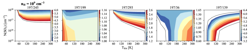
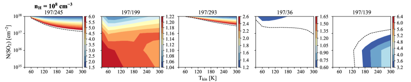
Figure 14: Comparison between observed intensity ratios and RADEX models. Top: Observed intensity ratios between SO₂ 18_4,14–18_3,15 (E_up = 197 K) and the other five transitions, above a 3$\sigma$ level. The synthesized beam is shown by the black filled ellipse in the bottom left corner of the first panel and the yellow star indicates the position of the source. Center: Intensity ratios from RADEX for the same transitions and employing a H₂ number density of 10⁹ cm^-3. Bottom: Same analysis from RADEX, but employing a H₂ number density of 10⁸ cm^-3. The black dashed contours indicate error values of 1$\sigma$ and the limits of the possible ranges. All values are possible for the panels without black dashed contours.

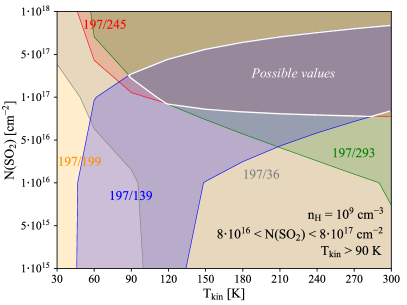
Figure 15: Range of possible values for the SO₂ column density and the kinetic temperature (white contours) from the overlap of the observed ranges in Fig. 14 (for a H₂ number density of 10⁹ cm^-3), indicated in different colors.

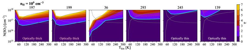
Figure 16: Optical depth for the six SO₂ transitions obtained with RADEX with n_H = 10⁹ cm^-3. The cyan contour represents $\tau$ = 1 and the dashed gray contours indicate the range of possible values for N${}_{\mathrm{SO_{2}}}$ and T_kin shown in Fig. 15.