Annealing Optimization for Progressive Learning with Stochastic Approximation

Abstract

In this work, we introduce a learning model designed to meet the needs of applications in which computational resources are limited, and robustness and interpretability are prioritized. Learning problems can be formulated as constrained stochastic optimization problems, with the constraints originating mainly from model assumptions that define a trade-off between complexity and performance. This trade-off is closely related to over-fitting, generalization capacity, and robustness to noise and adversarial attacks, and depends on both the structure and complexity of the model, as well as the properties of the optimization methods used. We develop an online prototype-based learning algorithm based on annealing optimization that is formulated as an online gradient-free stochastic approximation algorithm. The learning model can be viewed as an interpretable and progressively growing competitive-learning neural network model to be used for supervised, unsupervised, and reinforcement learning. The annealing nature of the algorithm contributes to minimal hyper-parameter tuning requirements, poor local minima prevention, and robustness with respect to the initial conditions. At the same time, it provides online control over the performance-complexity trade-off by progressively increasing the complexity of the learning model as needed, through an intuitive bifurcation phenomenon. Finally, the use of stochastic approximation enables the study of the convergence of the learning algorithm through mathematical tools from dynamical systems and control, and allows for its integration with reinforcement learning algorithms, constructing an adaptive state-action aggregation scheme.

I Introduction

Learning from data samples has proven to be an important component in the advancement of diverse fields, including artificial intelligence, computational physics, biological sciences, communication frameworks, and cyber-physical control systems. While virtually all learning problems can be formulated as constrained stochastic optimization problems, the optimization methods can be intractable, with the constraints originating mainly from model assumptions and defining a trade-off between complexity and performance [1]. For this reason, designing models of appropriate structure, and optimization methods with particular properties, has been the cornerstone of machine learning algorithms.

Currently, deep learning methods dominate the field of machine learning owing to their experimental performance in numerous applications [2]. However, they typically consist of overly complex models of a great many parameters, which comes in the expense of time, energy, data, memory, and computational resources [3, 4]. Furthermore, they are inherently uninterpretable and vulnerable to small perturbations [5, 6],which has led to an emerging hesitation in their usage outside common benchmark datasets and real-life or security critical applications [7].

In this work, we introduce a learning model designed to alleviate these limitations to meet the needs of applications in which computational resources are limited and robustness and interpretability are prioritized. To that end, the learning model should create a meaningful representation, should be updated recursively (and even in real time) with easy-to-implement updates, and its complexity should be appropriately and progressively adjusted to offer online control over the trade-off between model complexity and performance. This trade-off is also closely related to over-fitting, generalization capacity, and robustness to input perturbations and adversarial attacks [8]. This is further reinforced by recent studies revealing that existing flaws in the current benchmark datasets may have inflated the need for overly complex models [9], and that over-fitting to adversarial training examples may actually hurt generalization [10].

We focus on prototype-based models [11, 12, 13], which are iterative, consistent [11], interpretable, robust [14], and topology-preserving competitive-learning neural networks [15], sparse in the sense of memory complexity, fast to train and evaluate, and have recently shown impressive robustness against adversarial attacks, suggesting suitability in security critical applications [16]. They use a set of representatives (typically called prototypes, or codevectors) to partition the input space in an optimal way according to an appropriately defined objective function. This is an intuitive approach which parallels similar concepts from cognitive psychology and neuroscience. We approximate the global minima of the objective function by solving a sequence of optimization sub-problems that make use of entropy regularization at different levels. This is a deterministic annealing approach [12, 17] that (a) adjusts the number of prototypes/neurons (which defines the complexity of the model) as needed through an intuitive bifurcation phenomenon, (b) offers robustness with respect to the initial conditions, and (c) generalizes the proximity measures used to quantify the similarity between two vectors in the data space beyond convex metrics. In addition, the annealing nature of the algorithm contributes to (but does not guarantee) avoiding poor local minima, requires minimal hyper-parameter tuning, and allows online control over the performance-complexity trade-off.

Although deterministic annealing approaches have been known for a while [17], an online optimization method for such architectures is an important development, similar to the introduction of a greedy online training algorithm for a network of restricted Boltzmann machines that gave rise to one of the first effective deep learning algorithms [18]. We develop an online training rule based on a stochastic approximation algorithm [19, 20] and show that it is also gradient-free, provided that the proximity measure used belongs to the family of Bregman divergences: information-theoretic dissimilarity measures that play an important role in learning applications and include the widely used Euclidean distance and Kullback-Leibler divergence [21, 22]. While stochastic approximation offers an online, adaptive, and computationally inexpensive optimization framework, it is also strongly connected to dynamical systems. This enables the study of the convergence of the learning algorithm through mathematical tools from dynamical systems and control [20]. We take advantage of this property to prove the consistency of the proposed learning algorithm as a density estimator (unsupervised learning), and as a classification rule (supervised learning). Moreover, we make use of the theory of two-timescale stochastic approximation to show that the proposed learning algorithm can be used as an adaptive aggregation scheme in reinforcement learning settings with: (a) a fast component that executes a temporal-difference learning algorithm, and (b) a slow component for adaptive aggregation of the state-action space. Finally, we illustrate the properties and evaluate the performance of the proposed learning algorithm in multiple experiments.

In particular, we start by dedicating Section II to reviewing the theory of stochastic approximation as an optimization approach for learning algorithms, giving emphasis to its connection to dynamical systems. This concise background is targeted towards broader audience and aims to motivate the generalization of training updates in learning algorithms. We follow with Section III, where we introduce the Online Deterministic Annealing (ODA) algorithm for unsupervised and supervised learning and study its convergence and practical implementation. In Section IV we show how ODA can be integrated with common reinforcement learning approaches, and in particular as an adaptive state-action aggregation algorithm that allows Q-learning to be applied to Markov decision processes with infinite-dimensional state and input spaces. Finally, Section V illustrates experimental results, and Section VI concludes the paper.

II Stochastic Approximation: Learning with Dynamical Systems

In this section we briefly review the theory of stochastic approximation which is going to form the base for the convergence analysis of the proposed learning schemes. We give emphasis to its connection to dynamical systems, and how this property can be particularly useful to optimization and machine learning algorithms.

II-A Stochastic Approximation and Dynamical Systems

Stochastic approximation, first introduced in [19], was originally conceived as a tool for statistical computation, and, since then, has become a central tool in a number of different disciplines, often times unbeknownst to the users, researchers and practitioners. Stochastic approximation offers an online, adaptive, and computationally inexpensive optimization framework, properties that make it an ideal optimization method for machine learning algorithms. As a result, many of the most widely used learning algorithms partially or entirely consist of stochastic approximation algorithms; from stochastic gradient descent used in the back-propagation algorithm to train artificial neural networks [23, 24], to the Q-learning algorithm used in reinforcement learning applications [25, 26].

In addition to its connection with optimization and learning algorithms, stochastic approximation is also strongly connected to dynamical systems. A fact that is often overlooked is that almost any recursive numerical algorithm can be described by a discrete time dynamical system. In this sense, results about the behavior, e.g. stability and convergence properties, of discrete time dynamical systems can be applied to iterative optimization and learning algorithms. This connection is remarkably direct in stochastic approximation which allows the study of its convergence through the analysis of an ordinary differential equation, as illustrated in the following theorem, proven in [20]:

Theorem 1 ([20], Ch.2).

Almost surely, the sequence $\left\{x_{n}\right\}\in S\subseteq\mathbb{R}^{d}$ generated by the following stochastic approximation scheme:

$$x_{n+1}=x_{n}+\alpha(n)\left[h(x_{n})+M_{n+1}\right],\ n\geq 0$$ (1)

with prescribed $x_{0}$, converges to a (possibly sample path dependent) compact, connected, internally chain transitive, invariant set of the o.d.e:

$$\dot{x}(t)=h\left(x(t)\right),~{}t\geq 0,$$ (2)

where $x:\mathbb{R}_{+}\rightarrow\mathbb{R}_{d}$ and $x(0)=x_{0}$, provided the following assumptions hold:

• The map $h:\mathbb{R}^{d}\rightarrow\mathbb{R}^{d}$ is Lipschitz in $S$, i.e., $\exists L$ with $0<L<\infty$ such that $\left\|h(x)-h(y)\right\|\leq L\left\|x-y\right\|,~{}x,y\in S$,

• The stepsizes $\left\{\alpha(n)\in\mathbb{R}_{++},~{}n\geq 0\right\}$ satisfy $\sum_{n}\alpha(n)=\infty$, and $\sum_{n}\alpha^{2}(n)<\infty$ ,

• $\left\{M_{n}\right\}$ is a martingale difference sequence with respect to the increasing family of $\sigma$-fields $\mathcal{F}_{n}:=\sigma\left(x_{m},M_{m},~{}m\leq n\right)$, ${n\geq 0}$, i.e., $\mathbb{E}\left[M_{n+1}|\mathcal{F}_{n}\right]=0~{}a.s.$, for all $n\geq 0$, and, furthermore, $\left\{M_{n}\right\}$ are square-integrable with $\mathbb{E}\left[\left\|M_{n+1}\right\|^{2}|\mathcal{F}_{n}\right]\leq K\left(1+\left\|x_{n}\right\|^{2}\right),~{}a.s.$, where $n\geq 0$ for some $K>0$,

• The iterates $\left\{x_{n}\right\}$ remain bounded a.s., i.e., ${\sup_{n}\left\|x_{n}\right\|<\infty}$ $a.s.$

Intuitively, the stochastic process (1) can be seen as a noisy discretization (also known as Euler scheme in numerical analysis literature) of (2). As an immediate result, the following corollary also holds:

Corollary 1.1 ([20]).

If the only internally chain transitive invariant sets for (2) are isolated equilibrium points, then, almost surely, $\left\{x_{n}\right\}$ converges to a, possibly sample dependent, equilibrium point of (2).

Given the conditions of Theorem 1 and using standard Lyapunov arguments, the following corollary, regarding distributed, asynchronous implementation of the algorithm, also holds:

Corollary 1.2 ([20], Ch. 7).

Suppose there exists a continuously differentiable function $J$, such that $h(x)=-\nabla J(x)$ (or $h(x)=F(x)-x$). Define $Y_{n}\subseteq\left\{1,\ldots,d\right\}$ to be the subset of components of $x_{n}$ that are updated at time $n$, and $v(i,n):=\sum_{m=0}^{n}\mathds{1}_{\left[i\in Y_{m}\right]}$ to be the number of times the $i$-th component $x_{n}^{(i)}$ has been updated up until time $n$. Then, almost surely, the sequence $\left\{x_{n}\right\}$ generated by

$$x_{n+1}^{(i)}=x_{n}^{(i)}+\alpha(v(i,n))\mathds{1}_{[i\in Y_{n}]}\left[h^{(i)}(x_{n})+M_{n+1}^{(i)}\right]$$ (3)

where $i\in\left\{1,\ldots,d\right\}$, and $n\geq 0$, converge to the invariant set $H:=\left\{x:\nabla J(x)=0\right\}$ (or $H:=\left\{x:F(x)=x\right\}$), provided that each component $(i)$ is updated infinitely often, i.e.

$$\lim_{n\rightarrow\infty}\inf\frac{v(i,n)}{n}>0.$$

Corollaries 1.1 and 1.2, reveal the connection of the stochastic approximation algorithms with iterative approximation and optimization algorithms, including two notable special cases: stochastic gradient descent, and the Q-learning algorithm These special cases of stochastic approximation, are discussed in more detail in what follows.

II-B Stochastic Gradient Descent

Stochastic gradient descent is an iterative stochastic optimization method that tries to solve the problem of minimizing the cost:

$$\min_{\theta}\mathbb{E}\left[J(X,\theta)\right]$$ (4)

where $X:\Omega\rightarrow H$ is a random variable defined in the probability space $(\Omega,\mathcal{F},\mathbb{P})$, and $H$ is a Hilbert space. The update

$$\theta_{n+1}=\theta_{n}-\alpha_{n}\nabla_{\theta}J(x_{n},\theta_{n})$$ (5)

is used to bypass the estimation of $\mathbb{\hat{E}}\left[J(x,\theta_{n})\right]=\frac{1}{n}\sum_{i=1}^{n}J(x_{i},\theta_{n})$ which can be expensive or infeasible. This is a special case of a stochastic approximation update. Observe that, under the condition $\nabla_{\theta}\mathbb{E}\left[J(x,\theta_{n})\right]=\mathbb{E}\left[\nabla_{\theta}J(x,\theta_{n})\right]$, (5) can be written as:

$$\theta_{n+1}=\theta_{n}+\alpha_{n}\left[-\nabla_{\theta}\mathbb{E}\left[J\right]+(\mathbb{E}\left[\nabla_{\theta}J\right]-\nabla_{\theta}J)\right]$$ (6)

where $h(\theta)=-\nabla_{\theta}\mathbb{E}\left[J(X,\theta)\right]$ is a Lipschitz continuous function, and $M_{n}=\mathbb{E}\left[\nabla_{\theta}J(X,\theta)\right]-\nabla_{\theta}J(x_{n},\theta)$ is a martingale difference sequence, since the data samples $x_{n}$ are assumed independent realizations of the random variable $X$. Therefore by Theorem 1 and Corollary 1.1, as long as $\sum_{n}\alpha(n)=\infty$, and $\sum_{n}\alpha^{2}(n)<\infty$, and $\theta_{n}$ remain bounded a.s., stochastic gradient descent will converge to a possibly path dependent equilibrium of $\dot{\theta}=-\nabla_{\theta}\mathbb{E}\left[J(X,\theta)\right]$, i.e., in a minimizer of $\mathbb{E}\left[J(X,\theta)\right]$.

II-C Q-learning

As a second example, the Q-learning algorithm, widely used in reinforcement learning, is again a special case of a stochastic approximation algorithm [27]. Consider a discrete-time Markov Decision Process (MDP) $(\mathcal{X},\mathcal{U},\mathcal{P},C)$ with:

• $\mathcal{X}$ being the state space,

• $\mathcal{U}$ being the action (control) space,

• $\mathcal{P}:(x,u,x^{\prime})\mapsto\mathbb{P}\left[x^{\prime}|x,u\right]$ being the transition probabilities associated with a stochastic state transition function ${f:(x,u)\mapsto x^{\prime}}$, and

• $C:\mathcal{X}\times\mathcal{U}\rightarrow\mathbb{R}_{+}$, being the immediate cost function, assumed deterministic.

Reinforcement Learning (RL) examines the problem of learning a control policy $u:=(u_{0},u_{1},\ldots)$ that solves the discounted infinite-horizon optimal control problem

$$\min_{u}\mathbb{E}\left[\sum_{l=0}^{\infty}\gamma^{l}C(x_{l},u_{l})\right]$$

where $\gamma\in(0,1]$. Define the value function $V^{u}$ of a policy $u$ as

$$V^{u}(x_{k}): =\mathbb{E}\left[\sum_{l=k}^{\infty}\gamma^{l-k}C(x_{l},u_{l})\right]$$

$$=C(x_{k},u_{k})+\gamma\mathbb{E}\left[V^{u}(x_{k+1})\mid x_{k}\right]$$

$$=Q^{u}(x_{k},u_{k})$$

where $Q^{u}$ represents the quality function of a policy $u$, i.e. the expected return for taking action $u_{k}$ at time $k$ and state $x_{k}$, and thereafter following policy $u$. As a result of Bellman’s principle, we get the (discrete-time) Hamilton-Jacobi-Bellman (HJB) equation

$$V^{*}(x_{k}): =\min_{u}~{}\mathbb{E}\left[\sum_{l=k}^{\infty}\gamma^{l-k}C(x_{l},u_{l})\right]$$ (7)

$$\overset{(HJB)}{=}\min_{u}\left\{~{}C(x_{k},u_{k})+\gamma\mathbb{E}\left[V^{*}(x_{k+1})\mid x_{k}\right]~{}\right\}$$

$$=\min_{u_{k}}Q^{*}(x_{k},u_{k})$$

where $V^{*}:=V^{u^{*}}$ and $Q^{*}:=Q^{u^{*}}$ represent the optimal value and $Q$ functions, respectively. Reinforcement learning algorithms consist mainly of temporal-difference learning algorithms that try to approximate a solution to (7) using iterative optimization methods. The optimization is performed over a finite set of parameters which are used to describe the value (or Q) function. These parameters typically correspond to a parametric model (e.g. a neural network) used for function approximation, or to the different values of the vector $V(\mathcal{X})$ (or $Q(\mathcal{X},\mathcal{U})$), in which case $\mathcal{X}$ and $\mathcal{U}$ are assumed finite either by definition or as a result of discretization. Assuming that the state and action spaces $\mathcal{X}$ and $\mathcal{U}$ are finite, a widely used approach is the $Q$-learning algorithm:

$$Q_{j+1}(x,u^{\prime}) =Q_{j}(x,u^{\prime})+\alpha_{j}[C(x,u^{\prime})$$

$$~{}~{}~{}~{}~{}~{}~{}~{}~{}~{}~{}~{}~{}+\gamma\min_{u}Q_{j}(x^{\prime},u)-Q_{j}(x,u^{\prime})]$$

which is a stochastic approximation algorithm [27]:

$$Q_{j+1}(x,u^{\prime})=Q_{j}(x,u^{\prime})+\alpha_{j}[$$ (8)

$$~{}~{}\left(C(x,u^{\prime})+\gamma\mathbb{E}\left[\min_{u}Q_{j}(x,u)\right]-Q_{j}(x,u^{\prime})\right)$$

$$~{}~{}+\gamma\left(\min_{u}Q_{j}(x^{\prime},u)-\mathbb{E}\left[\min_{u}Q_{j}(x,u)\right]\right)]$$

with $h(Q(x,u^{\prime}))=C(x,u^{\prime})+\gamma\mathbb{E}\left[\min_{u}Q_{j}(x,u)\right]-Q_{j}(x,u^{\prime})$, and $M_{j}=\gamma\left(\min_{u}Q_{j}(x^{\prime},u)-\mathbb{E}\left[\min_{u}Q_{j}(x,u)\right]\right)$ is a martingale difference sequence. As a result, under the conditions of Theorem 1, the Q-learning algorithm converges to the global equilibrium of $\dot{Q}=F(Q)-Q$, with $F(Q(x,u^{\prime}))=C(x,u^{\prime})+\gamma\mathbb{E}\left[\min_{u}Q_{j}(x,u)\right]$, i.e., to the stationary point $Q(x,u)=C(x,u)+\gamma\mathbb{E}\left[\min_{u}Q_{j}(x,u)\right]$, which solves the Hamilton-Jacobi-Bellman equation.

II-D Dynamics and Control for Learning

It follows from the above that stochastic approximation algorithms define a family of iterative approximation and optimization algorithms that can be used, among others, for machine learning applications. Their strong connection to dynamical systems (see Theorem 1), can give rise to the study of learning algorithms and representations through systems-theoretic mathematics, connecting machine learning with stochastic optimization, adaptive control and dynamical systems, which can lead to new developments in the field of machine learning. As a first example, notice that (1) defines an iterative algorithm that can be used for stochastic optimization and does not necessarily depend on the gradient of a cost function. As will be shown in Section III, this can lead to gradient-free learning algorithms that can alleviate common problems such as that of the vanishing gradients.

In addition, the developed mathematical theory of dynamical systems can be utilized to construct and study learning algorithms that run at the same time but at different timescales. In particular, the theory of the O.D.E. method for stochastic approximation in two timescales as detailed in [20] is summarized in the following theorem:

Theorem 2 (Ch. 6 of [28]).

Consider the sequences $\left\{x_{n}\right\}\in S\subseteq\mathbb{R}^{d}$ and $\left\{y_{n}\right\}\in\Sigma\subseteq\mathbb{R}^{k}$, generated by the iterative stochastic approximation schemes:

$$x_{n+1}=x_{n}+\alpha(n)\left[f(x_{n},y_{n})+M_{n+1}^{(x)}\right]$$ (9)

$$y_{n+1}=y_{n}+\beta(n)\left[g(x_{n},y_{n})+M_{n+1}^{(y)}\right]$$ (10)

for $n\geq 0$ and $M_{n}^{(x)}$, $M_{n}^{(y)}$ martingale difference sequences, and assume that $\sum_{n}\alpha(n)=\sum_{n}\beta(n)=\infty$, $\sum_{n}(\alpha^{2}(n)+\beta^{2}(n))<\infty$, and $\nicefrac{{\beta(n)}}{{\alpha(n)}}\rightarrow 0$, with the last condition implying that the iterations for $\left\{y_{n}\right\}$ run on a slower timescale than those for $\left\{x_{n}\right\}$. If the equation

$$\dot{x}(t)=f(x(t),y),\ x(0)=x_{0}$$

has an asymptotically stable equilibrium $\lambda(y)$ for fixed $y$ and some Lipschitz mapping $\lambda$, and the equation

$$\dot{y}(t)=g(\lambda(y(t)),y(t)),\ y(0)=y_{0}$$

has an asymptotically stable equilibrium $y^{*}$, then, almost surely, $(x_{n},y_{n})$ converges to $(\lambda(y^{*}),y^{*})$.

This result allows for two learning algorithms, that may depend on each other, to run online at the same time, but at different timescales. As will be shown in Section IV, a two-timescale stochastic approximation algorithm can be used for reinforcement learning with: (a) a fast component that executes a Q-learning algorithm, and (b) a slow component, that adaptively partitions the state-action space according to an appropriately defined dissimilarity measure.

III Online Deterministic Annealing for Unsupervised and Supervised Learning

To formulate the mathematics of a prototype-based learning model that progressively grows in size, it is convenient to start our analysis with the case of unsupervised learning, i.e., clustering and density estimation, and then show how these results generalize in the supervised case, i.e., in classification and regression, as well. In the context of unsupervised learning, the observations (data) are represented by a random variable $X:\Omega\rightarrow S$ defined in a probability space $\left(\Omega,\mathcal{F},\mathbb{P}\right)$, where $S\subseteq\mathbb{R}^{d}$ is the observation space (data space). The goal of prototype-based learning is to define a similarity measure $d:S\rightarrow ri(S)$ (where $ri(S)$ represents the relative interior of $S$) and a set of $K$ prototypes $\mu:=\left\{\mu_{i}\right\}_{i=1}^{K}$, $\mu_{i}\in ri(S)$, on the data space such that an average distortion measure is minimized, i.e.,

$$\min_{\mu}~{}J(\mu):=\mathbb{E}\left[\min_{i}d(X,\mu_{i})\right]$$ (11)

Here the similarity measure as well as the number of prototypes $K$ are predefined designer parameters. This process is equivalent to finding the most suitable model out of a set of $K$ local constant models, and results in a piecewise-constant approximation of the data space $S$. This representation has been used for clustering in vector quantization applications [11, 29], and, in the limit $K\rightarrow\infty$, can be used for density estimation.

To construct a learning algorithm that progressively increases the number of prototypes $K$ as needed according to different “levels of detail” (to be defined shortly) we will define a probability space over an infinite number of candidate models, and constraint their distribution using the maximum-entropy principle at different levels. As we will show, solving a sequence of optimization problems parameterized by a single parameter $T$ will result in a series of model distributions with a finite number of $K(T)$ values with non-zero probability, i.e., this process results in a finite number of “effective codevectors” $K(T)$ that depends on a “temperature parameter” $T$.

First we need to adopt a probabilistic approach for (11), in which a quantizer $Q:S\rightarrow ri(S)$ is defined as a discrete random variable with domain $\mu:=\left\{\mu_{i}\right\}_{i=1}^{K}$, such that (11) becomes

$$\min_{\mu}~{}D(\mu) :=\mathbb{E}\left[d\left(X,Q\right)\right]$$ (12)

$$=\mathbb{E}\left[\mathbb{E}\left[d(X,Q)|X\right]\right]$$

$$=\int p(x)\sum_{i}p(\mu_{i}|x)d_{\phi}(x,\mu_{i})~{}dx$$

This is now a problem of finding the locations $\left\{\mu_{i}\right\}$ and the association probabilities $\left\{p(\mu_{i}|x)\right\}:=\left\{p(Q=\mu_{i}|X=x)\right\}$. Notice that this is a more general problem than that of (11), where it is subtly assumed that $p(\mu_{i}|x)=\mathds{1}_{\left[x\in S_{i}\right]}$, where $S_{i}=\left\{x\in S:i=\operatorname*{arg\,min}\limits_{j=1,\ldots,K}~{}d(x,\mu_{j})\right\},\ i=1,\ldots,K$, and $\left\{S_{i}\right\}$ defines a Voronoi partition.

Now, we make the assumption that we have access to an infinite number of possible models, i.e., that the quantizer $Q$ is a discrete random variable over a countably infinite set $\mu:=\left\{\mu_{i}\right\}$. Instead of choosing $K$ a priori, we will constraint the model distribution at different levels by maximizing the entropy:

$$H(\mu) :=\mathbb{E}\left[-\log P(X,Q)\right]$$ (13)

$$=H(X)+H(Q|X)$$

$$=H(X)-\int p(x)\sum_{i}p(\mu_{i}|x)\log p(\mu_{i}|x)~{}dx$$

This is essentially a realization of the Jaynes’s maximum entropy principle [30]. We formulate the resulting multi-objective optimization as the minimization of the Lagrangian

$$\min_{\mu}F(\mu):=D(\mu)-TH(\mu)$$ (14)

where $T\in[0,\infty)$ acts as a Lagrange multiplier, and, as we will show, can be seen as a temperature coefficient in an annealing process [12, 17].

Remark 1.

Alternatively, (14) can be formulated as

$$\min_{\mu}F(\mu):=(1-\lambda)D(\mu)-\lambda H(\mu)$$ (15)

where $\lambda\in\left[0,1\right]$, with

$$T:=\frac{1-\lambda}{\lambda},\quad\lambda\in\left[0,1\right]$$ (16)

representing the corresponding temperature coefficient. This is a mathematically equivalent formulation that, as will be discussed, can yield major benefits in the algorithmic implementation.

Equation (14) represents the scalarization method for trade-off analysis between two performance metrics, one related to performance, and one to generalization. The entropy $H$, acts as a regularization term, and is given progressively less weight as $T$ decreases. For large values of $T\rightarrow\infty$ we maximize the entropy. As we will show, this results in a unique effective codevector that represents the entire data space. As $T$ is lowered, we essentially transition from one solution of the multi-objective optimization (a Pareto point when the objectives are convex) to another in a naturally occurring direction that resembles an annealing process.

In this sense, the value of $T$ defines the “level of detail” of the dataset that is allowed to be seen by the maximum-entropy constraint. As we will show, when certain critical values of $T$ are reached, a bifurcation phenomenon occurs, according to which, the the number of non-zero values $K(T)$ of the model distribution increases, indicating that the solution to the optimization problem of minimizing $F(T)$ requires more “effective codevectors” $K(T)$.

Remark 2.

We note that this concept is similar to convex relaxation of hierarchical clustering, which results in a family of objective functions with a natural geometric interpretation [31]. However, as we will show, the proposed approach does not make any relaxation assumptions, uses entropy as a naturally occurring regularization term, and allows for the development of a gradient-free training rule based on stochastic approximation. This will result in a learning algorithm that can be integrated with reinforcement learning approaches.

III-A Solving the Optimization Problem

As in the case of standard vector quantization algorithms, we will minimize $F$ by successively minimizing it first respect to the association probabilities $\left\{p(\mu_{i}|x)\right\}$, and then with respect to the codevector locations $\mu$.

The following lemma provides the solution of minimizing $F$ with respect to the association probabilities $p(\mu_{i}|x)$:

Lemma 1.

The solution of the optimization problem

$$F^{*}(\mu) :=\min_{\left\{p(\mu_{i}|x)\right\}}F(\mu)$$ (17)

s.t. $$\sum_{i}p(\mu_{i}|x)=1$$

is given by the Gibbs distributions

$$p^{*}(\mu_{i}|x)=\frac{e^{-\frac{d(x,\mu_{i})}{T}}}{\sum_{j}e^{-\frac{d(x,\mu_{j})}{T}}},~{}\forall x\in S$$ (18)

Proof.

We form the Lagrangian:

$$\mathcal{L}_{f}(\left\{p(\mu_{i}|x)\right\},\nu) :=D(\mu)-TH(\mu)+\nu\left(\sum_{i}p(\mu_{i}|x)-1\right)$$ (19)

Taking $\frac{\partial\mathcal{L}}{\partial p(\mu|x)}=0$ yields:

$$d(x,\mu_{i})+T(1+\log p(\mu_{i}|x))+\nu=0$$ (20)

$$\implies\log p(\mu_{i}|x)=-\frac{1}{T}d(x,\mu_{i})-\left(1+\frac{\nu}{T}\right)$$

$$\implies p(\mu_{i}|x)=\frac{e^{-\frac{d(x,\mu_{i})}{T}}}{e^{1+\frac{\nu}{T}}}$$

Finally, from the condition $\sum_{i}p(\mu_{i}|x)=1$, it follows that

$$e^{1+\frac{\nu}{\lambda}}=\sum_{i}e^{-\frac{d(x,\mu_{i})}{T}}$$ (21)

which completes the proof. ∎

In order to minimize $F^{*}(\mu)$ with respect to the codevector locations $\mu$ we set the gradients to zero

$$\frac{d}{d\mu}F^{*}(\mu)=0\implies\frac{d}{d\mu}\left(D(\mu)-TH(\mu)\right)=0$$ (22)

$$\implies\int p(x)\sum_{i}\frac{d}{d\mu}\left(p^{*}(\mu_{i}|x)d_{\phi}(x,\mu_{i})\right)$$

$$\quad\quad\quad+T\frac{d}{d\mu}\left(p^{*}(\mu_{i}|x)\log p^{*}(\mu_{i}|x)\right)~{}dx=0$$

$$\implies\sum_{i}\int p(x)p^{*}(\mu_{i}|x)\frac{d}{d\mu_{i}}d(x,\mu_{i})~{}dx=0$$

where we have used (18), direct differentiation, and the fact that $\sum_{i}\frac{d}{d\mu}p^{*}(\mu_{i}|x)=\frac{d}{d\mu}\sum_{i}p^{*}(\mu_{i}|x)=0$. In the next section, we show that (22) has a closed form solution if the dissimilarity measure $d$ belongs to the family of Bregman divergences.

III-B Bregman Divergences as Dissimilarity Measures

Prototype-based algorithms rely on measuring the proximity between different vector representations. In most cases the Euclidean distance or another convex metric is used, but this can be generalized to alternative dissimilarity measures inspired by information theory and statistical analysis, such as the Bregman divergences [21]:

Definition 1 (Bregman Divergence).

Let $\phi:H\rightarrow\mathbb{R}$, be a strictly convex function defined on a vector space $H$ such that $\phi$ is twice F-differentiable on $H$. The Bregman divergence $d_{\phi}:H\times H\rightarrow\left[0,\infty\right)$ is defined as:

$$d_{\phi}\left(x,\mu\right)=\phi\left(x\right)-\phi\left(\mu\right)-\frac{\partial\phi}{\partial\mu}\left(\mu\right)\left(x-\mu\right),$$

where $x,\mu\in H$, and the continuous linear map $\frac{\partial\phi}{\partial\mu}\left(\mu\right):H\rightarrow\mathbb{R}$ is the Fréchet derivative of $\phi$ at $\mu$.

In this work, we will concentrate on nonempty, compact convex sets $S\subseteq\mathbb{R}^{d}$ so that the derivative of $d_{\phi}$ with respect to the second argument can be written as

$$\frac{\partial d_{\phi}}{\partial\mu}(x,\mu) =\frac{\partial\phi(x)}{\partial\mu}-\frac{\partial\phi(\mu)}{\partial\mu}-\frac{\partial^{2}\phi(\mu)}{\partial\mu^{2}}(x-\mu)+\frac{\partial\phi(\mu)}{\partial\mu}$$ (23)

$$=-\frac{\partial^{2}\phi(\mu)}{\partial\mu^{2}}(x-\mu)=-\left<\nabla^{2}\phi(\mu),(x-\mu)\right>$$ (24)

where $x,\mu\in S$, $\frac{\partial}{\partial\mu}$ represents differentiation with respect to the second argument of $d_{\phi}$, and $\nabla^{2}\phi(\mu)$ represents the Hessian matrix of $\phi$ at $\mu$.

Example 1.

As a first example, $\phi(x)=\left<x,x\right>,\ x\in\mathbb{R}^{d}$, yields the squared Euclidean distance $d_{\phi}(x,\mu)=\|x-\mu\|^{2}$.

Example 2.

A second interesting Bregman divergence that shows the connection to information theory, is the generalized I-divergence which results from $\phi(x)=\left<x,\log x\right>,\ x\in\mathbb{R}_{++}^{d}$ such that

$$d_{\phi}(x,y)=\left<x,\log x-\log\mu\right>-\left<\mathds{1},x-\mu,\right>$$

where $\mathds{1}\in\mathbb{R}^{d}$ is the vector of ones. It is easy to see that $d_{\phi}(x)$ reduces to the Kullback-Leibler divergence if $\left<\mathds{1},x\right>=1$.

The family of Bregman divergences provides proximity measures that have been shown to enhance the performance of a learning algorithm [22]. There is also a deeper connection of Bregman divergences to prototype-based learning algorithms [21]. In the next theorem, we show that we can have analytical solution to the last optimization step (22) in a convenient centroid form, if $d$ is a Bregman divergence.

Theorem 3.

The optimization problem

$$\min_{\mu}F^{*}(\mu)$$ (25)

where $F^{*}(\mu)$ is defined in (17) is solved by the codevector locations $\mu$ given by

$$\mu_{i}^{*}=\mathbb{E}\left[X|\mu_{i}\right]=\frac{\int xp(x)p^{*}(\mu_{i}|x)~{}dx}{p^{*}(\mu_{i})}$$ (26)

if $d:=d_{\phi}$ is a Bregman divergence for some function $\phi$ that satisfies Definition 1.

Proof.

Given (24), (22) becomes

$$\int(x-\mu_{i})p(x)p^{*}(\mu_{i}|x)~{}dx=0$$ (27)

which is equivalent to (26) since $\int p(x)p^{*}(\mu_{i}|x)~{}dx=p^{*}(\mu_{i})$. ∎

III-C Bifurcation and The Number of Clusters

So far, we have assumed a countably infinite set of codevectors. In this section we will show that the distribution of the quantizer $Q$ is actually discrete and takes values from a finite set of $K(T)$ codevectors which we call “effective codevectors”. Both the number and the locations of the codevectors will depend on the value of the temperature parameter $T$. These effective codevectors are the only parameters that an algorithmic implementation will need to store in memory.

First, notice that as $T\rightarrow\infty$, equation (18) yields uniform association probabilities $p(\mu_{i}|x)=p(\mu_{j}|x),\ \forall i,j,\forall x$. As a result of (26), all codevectors are located at the same point:

$$\mu_{i}=\mathbb{E}\left[X\right],\ \forall i$$

which means that there is one unique effective codevector given by $\mathbb{E}\left[X\right]$.

As $T$ is lowered below a critical value, a bifurcation phenomenon occurs, when the number of effective codevectors increases, which is a physical analogy with chemical annealing processes. Mathematically, it occurs when the existing solution $\mu^{*}$ given by (26) is no longer the minimum of the free energy $F^{*}$, as the temperature $T$ crosses a critical value. Following principles from variational calculus, we can rewrite the necessary condition for optimality (22) as

$$\frac{d}{d\epsilon}F^{*}(\mu+\epsilon\psi)|_{\epsilon=0}=0$$ (28)

with the second order condition being

$$\frac{d^{2}}{d\epsilon^{2}}F^{*}(\left\{\mu+\epsilon\psi\right\})|_{\epsilon=0}\geq 0$$ (29)

for all choices of finite perturbations $\left\{\psi\right\}$. Here we will denote by $\left\{y:=\mu+\epsilon\psi\right\}$ a perturbed codebook, where $\psi$ are perturbation vectors applied to the codevectors $\mu$, and $\epsilon\geq 0$ is used to scale the magnitude of the perturbation. Bifurcation occurs when equality is achieved in (29) and hence the minimum is no longer stable. These conditions are described in the following theorem:

Theorem 4.

Bifurcation occurs under the following condition

$$\exists y_{n}\text{ s.t. }p(y_{n})>0\text{ and }\det\left[I-T\frac{\partial^{2}\phi(y_{n})}{\partial y_{n}^{2}}C_{x|y_{n}}\right]=0$$ (30)

where $C_{x|y_{n}}:=\mathbb{E}\left[(x-y_{n})(x-y_{n})^{\mathrm{T}}|y_{n}\right]$.

Proof.

From direct differentiation the optimality condition (29) becomes

$$\sum_{i}p(y_{i})\frac{\partial^{2}\phi(y_{i})}{\partial y_{i}^{2}}\psi^{\mathrm{T}}\left[I-T\frac{\partial^{2}\phi(y_{i})}{\partial y_{i}^{2}}C_{x|y_{i}}\right]\psi$$ (31)

$$\quad+T\int p(x)\left(\sum_{i}p(y_{i}|x)\frac{\partial^{2}\phi(y_{i})}{\partial y_{i}^{2}}(x-y_{i})^{\mathrm{T}}\psi\right)^{2}dx=0$$

where

$$C_{x|y_{i}}:=\mathbb{E}\left[(x-y_{i})(x-y_{i})^{\mathrm{T}}|y_{i}\right]=\int p(x|y_{i})(x-y_{i})(x-y_{i})^{\mathrm{T}}dx$$ (32)

The left-hand side of (31) is positive for all perturbations $\left\{\psi\right\}$ if and only if the first term is positive. To see that, notice that the second term of (31) is clearly non-negative. For the left-hand side to be non-positive, the first term needs to be non-positive as well, i.e., there should exist at least one codevector value, say $y_{n}$, such that $p(y_{n})>0$ and $\left[I-T\frac{\partial^{2}\phi(y_{n})}{\partial y_{n}^{2}}C_{x|y_{n}}\right]\preceq 0$. In this case, there always exist a perturbation vector $\left\{y\right\}$ such that $y=0$, $\forall y\neq y_{n}$, and $\sum_{y=y_{n}}\psi=0$, that vanishes the second term, i.e., $T\int p(x)\left(\sum_{i}p(y_{i}|x)\frac{\partial^{2}\phi(y_{i})}{\partial y_{i}^{2}}(x-y_{i})^{\mathrm{T}}\psi\right)^{2}dx=0$. In other words we have shown that

$$\frac{d^{2}}{d\epsilon^{2}}F^{*}(y)>0\Leftrightarrow$$ (33)

$$\quad\exists y_{n}\text{ s.t. }p(y_{n})>0\text{ and }\left[I-T\frac{\partial^{2}\phi(y_{n})}{\partial y_{n}^{2}}C_{x|y_{n}}\right]\succ 0$$

which completes the proof. ∎

Notice that loss of minimality also implies that the number of effective codevectors has changed, otherwise the minimum would be stable. In addition, we have showed that bifurcation depends on the temperature coefficient $T$ (and the choice of the Bregman divergence, through the function $\phi$) and occurs when

$$\frac{1}{T}=\frac{\partial^{2}\phi(y_{n})}{\partial y_{n}^{2}}\bar{\nu}$$ (34)

where $\bar{\nu}$ is the largest eigenvalue of $C_{x|y_{n}}$. As a result, the following corollary holds:

Corollary 4.1.

The number of effective codevectors always remains bounded between two critical temperature values.

In other words, an algorithmic implementation needs only as many codevectors as the number of effective codevectors, which depends only on changes of the temperature parameter below certain thresholds that depend on the dataset at hand and the dissimilarity measure used. As shown in Alg. 1, we can detect the bifurcation points by introducing perturbing pairs of codevectors at each temperature level $T$. In this way, the codevectors $\mu$ are doubled by inserting a perturbation of each $\mu_{i}$ in the set of effective codevectors. The newly inserted codevectors will merge with their pair if a critical temperature has not been reached and separate otherwise. For more details about the implementation of the algorithm the reader is referred to [12].

III-D The Online Learning Rule

The conditional expectation $\mathbb{E}\left[X|\mu\right]$ in eq. (26) can be approximated by the sample mean of the data points weighted by their association probabilities $p(\mu|x)$, i.e., $\mathbb{\hat{E}}\left[X|\mu\right]=\frac{\sum xp(\mu|x)}{p(\mu)}$. This approach, however, defines an offline (batch) optimization algorithm and requires the entire dataset to be available a priori, subtly assuming that it is possible to store and also quickly access the entire dataset at each iteration. This is rarely the case in practical applications and results to computationally costly iterations that are slow to converge.

We propose an Online Deterministic Annealing (ODA) algorithm, that dynamically updates its estimate of the effective codevectors with every observation. This results in a significant reduction in complexity, that comes in two levels. The first refers to huge reduction in memory complexity, since we bypass the need to store the entire dataset, as well as the association probabilities $\left\{p(\mu_{i}|x),\ \forall x,i\right\}$ that map each data point in the dataset to each cluster. The second level refers to the nature of the optimization iterations. In the online approach the optimization iterations increase in number but become much faster, and practical convergence is often reached after a smaller number of observations. To define an online training rule for the deterministic annealing framework, we formulate a stochastic approximation algorithm to recursively estimate $\mathbb{E}\left[X|\mu\right]$ directly. The following theorem provides a means towards constructing a gradient-free stochastic approximation training rule for the online deterministic annealing algorithm.

Theorem 5.

Let $S$ a vector space, $\mu\in S$, and $X:\Omega\rightarrow S$ be a random variable defined in a probability space $\left(\Omega,\mathcal{F},\mathbb{P}\right)$. Let $\left\{x_{n}\right\}$ be a sequence of independent realizations of $X$, and $\left\{\alpha(n)>0\right\}$ a sequence of stepsizes such that $\sum_{n}\alpha(n)=\infty$, and $\sum_{n}\alpha^{2}(n)<\infty$. Then the random variable $m_{n}=\nicefrac{{\sigma_{n}}}{{\rho_{n}}}$, where $(\rho_{n},\sigma_{n})$ are sequences defined by

$$\rho_{n+1} =\rho_{n}+\alpha(n)\left[p(\mu|x_{n})-\rho_{n}\right]$$ (35)

$$\sigma_{n+1} =\sigma_{n}+\alpha(n)\left[x_{n}p(\mu|x_{n})-\sigma_{n}\right],$$

converges to $\mathbb{E}\left[X|\mu\right]$ almost surely, i.e. $m_{n}\xrightarrow{a.s.}\mathbb{E}\left[X|\mu\right]$.

Proof.

We will use the facts that $p(\mu)=\mathbb{E}\left[p(\mu|x)\right]$ and $\mathbb{E}\left[\mathds{1}_{\left[\mu\right]}X\right]=\mathbb{E}\left[xp(\mu|x)\right]$. The recursive equations (35) are stochastic approximation algorithms of the form:

$$\rho_{n+1} =\rho_{n}+\alpha(n)[(p(\mu)-\rho_{n})+$$ (36)

$$\quad\quad\quad\quad\quad\quad\quad\quad(p(\mu|x_{n})-\mathbb{E}\left[p(\mu|X)\right])]$$

$$\sigma_{n+1} =\sigma_{n}+\alpha(n)[(\mathbb{E}\left[\mathds{1}_{\left[\mu\right]}X\right]-\sigma_{n})+$$

$$\quad\quad\quad\quad\quad\quad(x_{n}p(\mu|x_{n})-\mathbb{E}\left[x_{n}p(\mu|X)\right])]$$

It is obvious that both stochastic approximation algorithms satisfy the conditions of Theorem 1. As a result, they converge to the asymptotic solution of the differential equations

$$\dot{\rho} =p(\mu)-\rho$$

$$\dot{\sigma} =\mathbb{E}\left[\mathds{1}_{\left[\mu\right]}X\right]-\sigma$$

which can be trivially derived through standard ODE analysis to be $\left(p(\mu),\mathbb{E}\left[\mathds{1}_{\left[\mu\right]}X\right]\right)$. This follows from the fact that the only internally chain transitive invariant sets for (36) are the isolated equilibrium points $\left(p(\mu),\mathbb{E}\left[\mathds{1}_{\left[\mu\right]}X\right]\right)$. In other words, we have shown that

$$\left(\rho_{n},\sigma_{n}\right)\xrightarrow{a.s.}\left(p(\mu),\mathbb{E}\left[\mathds{1}_{\left[\mu\right]}X\right]\right)$$ (37)

The convergence of $m_{n}$ follows from the fact that $\mathbb{E}\left[X|\mu\right]=\nicefrac{{\mathbb{E}\left[\mathds{1}_{\left[\mu\right]}X\right]}}{{p(\mu)}}$, and standard results on the convergence of the product of two random variables. ∎

As a direct consequence of this theorem, the following corollary provides an online learning rule that solves the optimization problem of the deterministic annealing algorithm.

Corollary 5.1.

The online training rule

$$\begin{cases}\rho_{i}(n+1)&=\rho_{i}(n)+\alpha(n)\left[\hat{p}(\mu_{i}|x_{n})-\rho_{i}(n)\right]\\ \sigma_{i}(n+1)&=\sigma_{i}(n)+\alpha(n)\left[x_{n}\hat{p}(\mu_{i}|x_{n})-\sigma_{i}(n)\right]\end{cases}$$ (38)

where the quantities $\hat{p}(\mu_{i}|x_{n})$ and $\mu_{i}(n)$ are recursively updated as follows:

$$\hat{p}(\mu_{i}|x_{n}) =\frac{\rho_{i}(n)e^{-\frac{d(x_{n},\mu_{i}(n))}{T}}}{\sum_{i}\rho_{i}(n)e^{-\frac{d(x_{n},\mu_{i}(n))}{T}}}$$ (39)

$$\mu_{i}(n) =\frac{\sigma_{i}(n)}{\rho_{i}(n)},$$

converges almost surely to a possibly sample path dependent solution of the optimization (25), as $n\rightarrow\infty$.

Finally, the determinsitic annealing algorithm with the learning rule (38), (39) can be used to define a consistent (histogram) density estimator at the limit $T\rightarrow 0$. In the limit $\lambda\rightarrow 0$, and as the number of observed samples $\left\{x_{n}\right\}$ goes to infinity, i.e., $n\rightarrow\infty$, the learning algorithm based on (38), (39), results in a codevector $\mu$ that constructs a consistent density estimator. This follows from the fact that as $T\rightarrow 0$, we get $p^{*}(\mu_{i}|x)\rightarrow\mathds{1}_{\left[x\in S_{i}\right]}$ and $K\rightarrow\infty$, i.e., the number of effective codevectors $K$ goes to infinity. As a result, it can be shown that $Vol(S_{i})\rightarrow 0$, where $S_{i}=\left\{x\in S:i=\operatorname*{arg\,min}\limits_{j}~{}d(x,\mu_{j})\right\}$. Then, $\hat{p}(x)=\frac{\sum_{i}\mathds{1}_{\left[x\in S_{i}\right]}}{nVol(S_{i})}$ is a consistent density estimator. The proof follows similar arguments to the stochastic vector quantization algorithm (see, e.g., [32]) but is omitted due to space limitations.

III-E Online Deterministic Annealing for Supervised Learning

The same learning algorithm can be extended for classification as well. A multi-class classification problem involves a pair of random variables $\left\{X,c\right\}\in S\times S_{c}$ defined in a probability space $\left(\Omega,\mathcal{F},\mathbb{P}\right)$, with $c\in S_{c}$ representing the class of $X$ and $S\subseteq\mathbb{R}^{d}$. The codebook is represented by $\mu:=\left\{\mu_{i}\right\}_{i=1}^{K}$, $\mu_{i}\in ri(S)$, and $c_{\mu}:=\left\{c_{\mu_{i}}\right\}_{i=1}^{K}$, such that $c_{\mu_{i}}\in S_{c}$ represents the class of $\mu_{i}$ for all $i\in\left\{1,\ldots,K\right\}$.

We can approximate the optimal solution of a minimum classification error problem by using the distortion measure

$$d^{c}(x,c_{x},\mu,c_{\mu})=\begin{cases}d(x,\mu),~{}c_{x}=c_{\mu}\\ 0,~{}c_{x}\neq c_{\mu}\end{cases}$$ (40)

It is easy to see that this particular choice for the distortion measure $d^{c}$ in (40) transforms the learning rule in (38) to

$$\begin{cases}\rho_{i}(n+1)&=\rho_{i}(n)+\beta(n)\left[s_{i}\hat{p}(\mu_{i}|x_{n})-\rho_{i}(n)\right]\\ \sigma_{i}(n+1)&=\sigma_{i}(n)+\beta(n)\left[s_{i}x_{n}\hat{p}(\mu_{i}|x_{n})-\sigma_{i}(n)\right]\end{cases}$$ (41)

where $s_{i}:=\mathds{1}_{\left[c_{\mu_{i}}=c\right]}$. As a result, this is equivalent to estimating strongly consistent class-conditional density estimators:

$$\hat{p}(x|c=j)\rightarrow\pi_{j}p(x|c=j),\ a.s.$$ (42)

where $\pi_{i}:=\mathbb{P}\left[c=i\right]$. This results in a Bayes-optimal classification scheme. The proof is beyond the scope of this paper, since we will focus our attention to reinforcement learning. As a side note, a practical classification rule such as the nearest-neighbor rule:

$$\hat{c}(x)=c_{\mu_{h^{*}}}$$ (43)

where $h^{*}=\operatorname*{arg\,max}\limits_{\tau=1,\ldots,K}~{}p(\mu_{\tau}|x),~{}h\in\left\{1,\ldots,K\right\}$, results in an easy=to-implement classifier with tight upper bound, i.e., $J_{B}^{*}\leq\hat{J}_{B}^{*}\leq 2J_{B}^{*}$, where $J_{B}$ represents the optimal Bayes error (see, e.g., [32]).

III-F The Algorithm

The Online Deterministic Annealing (ODA) algorithm for both clustering and classification is shown in Algorithm 1 and its source code is publicly available. The temperature parameter $T_{i}$ is reduced using the geometric series $T_{i+1}=\gamma T_{i}$, for $\gamma<1$. The temperature schedule $\left\{T_{i}\right\}$ affects the behavior of the algorithm by introducing the following trade-off: small steps $T_{i}-T_{i-1}$ are theoretically expected to give better results, i.e., not miss any bifurcation points, but larger steps provide computational benefits.

Remark 3.

Notice that the temperature schedule and its values depend on the range of the domain of the data. When the input domain is not known a prior, we can use the formulation (15), and (16), substituting $T_{i}$ by $T_{i}:=\frac{1-\lambda_{i}}{\lambda_{i}},\quad\lambda_{i}\in\left[0,1\right].$

Regarding the stochastic approximation stepsizes, simple time-based learning rates of the form $\alpha_{n}=\nicefrac{{1}}{{a+bn}}$, $a,b>0$, have experimentally shown to be sufficient for fast convergence. Convergence is checked with the condition $Td_{\phi}(\mu_{i}^{n},\mu_{i}^{n-1})<\epsilon_{c}$ for a given threshold $\epsilon_{c}$. This condition becomes harder as the value of $T$ decreases. Exploring adaptive learning rates is among the authors’ future research direction. The stopping criteria $SC_{stop}$ can include a maximum number of codevectors $K_{max}$ allowed, a minimum temperature $T_{min}$ to be reached, a minimum distortion/classification error $e_{target}$ to be reached, a maximum number of iterations $i_{max}$ reached, and so on.

Bifurcation, at $T_{i}$, is detected by maintaining a pair of perturbed codevectors $\left\{\mu_{j}+\delta,\mu_{j}-\delta\right\}$ for each effective codevector $\mu_{j}$ generated by the algorithm at $T_{i-1}$, i.e. for $j=1\ldots,K_{i-1}$. Using arguments from variational calculus (see Section III-C), it is easy to see that, upon convegence, the perturbed codevectors will merge if a critical temperature has not been reached, and will get separated otherwise. Therefore, the cardinality of the model is at most doubled at every temperature level. These are the effective codevectors discussed in Section III-C. For classification, a perturbed codevector for each class is generated. Merging is detected by the condition $Td_{\phi}(\mu_{j},\mu_{i})<\epsilon_{n}$, where $\epsilon_{n}$ is a design parameter that acts as a regularization term for the model that controls the number of effective codevectors. These comparisons need not be in any specific order and the worst-case number of comparisons is $N_{k}=\sum_{i=1}^{K-1}i$, which scales with $O(K^{2})$. An additional regularization mechanism is the detection of idle codevectors, which is checked by the condition $\rho_{i}(n)<\epsilon_{r}$, where $\rho_{i}(n)$ can be seen as an approximation of the probability $p(\mu_{i},c_{\mu_{i}})$. In practice, $\epsilon_{c}$, $\epsilon_{n}$, $\epsilon_{r}$ are assigned similar values and their impact on the performance is similar to any threshold parameter that detects convergence.

The complexity of Alg. 1 for a fixed temperature coefficient $T_{i}$ is $O(N_{c_{i}}(2K_{i})^{2}d)$, where $N_{c_{i}}$ is the number of stochastic approximation iterations needed for convergence which corresponds to the number of data samples observed, $K_{i}$ is the number of codevectors of the model at temperature $T_{i}$, and $d$ is the dimension of the input vectors, i.e., $x\in\mathbb{R}^{d}$. Therefore, assuming a training dataset of $N$ samples and a temperature schedule $\left\{T_{1}=T_{max},T_{2},\ldots,T_{N_{T}}=T_{min}\right\}$, the worst case complexity of Algorithm 1 becomes:

$$O(N_{c}(2\bar{K})^{2}d)$$

where $N_{c}=\max_{i}\left\{N_{c_{i}}\right\}$ is an upper bound on the number of data samples observed until convergence at each temperature level, and

$$N_{T}\leq\bar{K}\leq\min\left\{\sum_{n=0}^{N_{T}-1}2^{n},\sum_{n=0}^{\log_{2}K_{max}}2^{n}\right\}<N_{T}K_{max}$$

where the actual value of $\bar{K}$ depends on the bifurcations occurred as a result of reaching critical temperatures and the effect of the regularization mechanisms described above. Note that typically $N_{c}\ll N$ as a result of the stochastic approximation algorithm, and $\bar{K}\ll N_{T}K_{max}$ as a result of the progressive nature of the ODA algorithm.

As a final note, because the convergence to the Bayes decision surface comes in the limit $(K,T)\rightarrow(\infty,0)$, in practice, a fine-tuning mechanism can be designed to run on top of Alg. 1 after a predefined threshold temperature $T_{min}$. This can be either an LVQ algorithm [33] or some other local model, i.e., we can use the partition created by Alg. 1 to train local models in each region of the data space.

Algorithm 1 Online Deterministic Annealing (ODA)

  Select a Bregman divergence $d_{\phi}$

  Set stopping criteria $SC_{stop}$ (e.g., $K_{max}$, $T_{min}$)

  Set convergence parameters: $\gamma$, $\left\{\alpha_{n}\right\}$, $\epsilon_{c}$, $\epsilon_{n}$, $\epsilon_{r}$, $\delta$

  Initialize: $K=1$, $\lambda=1-\epsilon$, $T=\nicefrac{{1-\lambda}}{{\lambda}}$, $\left\{\mu^{i}\right\}$, $\left\{c_{\mu^{i}}=c,~{}\forall c\in\mathcal{C}\right\}$, $\left\{p(\mu^{i})=1\right\}$, $\left\{\sigma(\mu^{i})=\mu^{i}p(\mu_{i})\right\}$

  repeat

     Perturb $\mu^{i}\leftarrow\left\{\mu^{i}+\delta,\mu^{i}-\delta\right\}$, $\forall i$

     Update $K\leftarrow 2K$, $p(\mu^{i})$, $\sigma(\mu^{i})\leftarrow\mu^{i}p(\mu^{i})$, $\forall i$

     $n\leftarrow 0$

     repeat

        Observe data point $x$ and class label $c$

        for $i=1,\ldots,K$ do

           Compute membership $s^{i}=\mathds{1}_{\left[c_{\mu^{i}}=c\right]}$

           Update:

$$p(\mu^{i}|x) \leftarrow\frac{p(\mu^{i})e^{-\frac{d_{\phi}(x,\mu^{i})}{T}}}{\sum_{j}p(\mu^{j})e^{-\frac{d_{\phi}(x,\mu^{j})}{T}}}$$

$$p(\mu^{i}) \leftarrow p(\mu^{i})+\alpha_{n}\left[s^{i}p(\mu^{i}|x)-p(\mu^{i})\right]$$

$$\sigma(\mu^{i}) \leftarrow\sigma(\mu^{i})+\alpha_{n}\left[s^{i}xp(\mu^{i}|x)-\sigma(\mu^{i})\right]$$

$$\mu^{i} \leftarrow\frac{\sigma(\mu^{i})}{p(\mu^{i})}$$

           $n\leftarrow n+1$

        end for

     until Convergence: $Td_{\phi}(\mu^{i}_{n},\mu^{i}_{n-1})<\epsilon_{c}$, $\forall i$

     Keep effective codevectors: discard $\mu^{i}$ if $Td_{\phi}(\mu^{j},\mu^{i})<\epsilon_{n}$, $\forall i,j,i\neq j$

     Remove idle codevectors: discard $\mu^{i}$ if $p(\mu^{i})<\epsilon_{r}$, $\forall i$

     Update $K$, $p(\mu^{i})$, $\sigma(\mu^{i})$, $\forall i$

     Lower temperature: $\lambda\leftarrow\gamma\lambda$, $T\leftarrow\frac{1-\lambda}{\lambda}$

  until $SC_{stop}$

IV Online Deterministic Annealing for Reinforcement Learning

The learning architecture of Alg. 1 can also be integrated with reinforcement learning methods, giving rise to adaptive state-action aggregation schemes. As will be shown in this section, this is a result of using stochastic approximation as a training rule, and yields a reinforcement learning algorithm based on a progressively changing underlying model [34, 35].

We consider an MDP $(\mathcal{X},\mathcal{U},\mathcal{P},C)$, where $S\subseteq\mathbb{R}^{d_{X}}$, $S\subseteq\mathbb{R}^{d_{U}}$ are compact convex sets (see Section II-C). We are interested in the approximation of the quality function $Q:\mathcal{X}\times\mathcal{U}\rightarrow\mathbb{R}_{+}$. To this end, we use the online deterministic annealing (ODA) algorithm (Alg. 1) as an online recursive algorithm that finds an optimal representation of the data space with respect to a trade-off between minimum average distortion and maximum entropy. We define a quantizer $Q_{P}(x,u)=\sum_{h=1}^{K}\mu_{h}\mathds{1}_{\left[(x,u)\in P_{h}\right]}$, where $\left\{P_{h}\right\}_{h=1}^{K}$ is a partition of $\mathcal{X}\times\mathcal{U}$. The parameters $\mu_{h}:=(m_{h},v_{h})$ define a state-action aggregation scheme with $K$ clusters (aggregate state-action pairs), each represented by $m_{h}\in\mathcal{X}$ and $v_{h}\in\mathcal{U}$, for $h=1,\ldots,K$. After convergence, if the representation is meaningful, the finite set $\left\{\mu_{h}\right\}_{h=1}^{K}$, where $\mu_{h}\in\mathcal{X}\times\mathcal{U}$, can be used directly as a piece-wise constant approximation of the $Q$ function. We stress that the cardinality $K$ of the set of representatives of the space $\mathcal{X}\times\mathcal{U}$ is automatically updated by Alg. 1 and progressively increases, as needed, with respect to the complexity-accuracy trade-off presented above.

Remark 4.

It is also possible to use $\left\{\mu_{h}\right\}_{h=1}^{K}$ as pseudo-inputs for an adaptive and sparse Gaussian process regression [36], but this is beyond the scope of this paper.

In essence, we are approximating the $Q$ function with a piece-wise constant parametric model with the parameters that define the partition living in the data space and being chosen by the online deterministic annealing algorithm (Alg. 1). However, since the system observes its states and actions online while learning its optimal policy using a temporal-difference reinforcement learning algorithm, the two estimation algorithms need to run at the same time. This can become possible by observing that Algorithm 1, as well as most temporal-difference algorithms, are stochastic approximation algorithms. Therefore, we can design a reinforcement learning algorithm as a two-timescale stochastic approximation algorithm with (a) a fast component that updates the values $Q:=\left\{Q(h)\right\}_{h=1}^{K}$ with a temporal-difference learning algorithm, and (b) a slow component that updates the representation $\mu:=\left\{\mu_{h}\right\}_{h=1}^{K}$ based on Alg. 1. Such a framework can incorporate different reinforcement learning algorithms, including the proposed algorithm presented in Alg. 2. The exploration policy $\pi_{L}(h|\mu)$ in Alg. 2 depends on the aggregate state $h$ and balances the ratio between exploration and exploitation.

Algorithm 2 Reinforcement Learning with ODA

  Initialize $\mu_{h}$, $Q_{0}(h)$, $\forall h\in\left\{1,\ldots,K\right\}$

  repeat

     Observe $x$ and find

$$h=\operatorname*{arg\,min}\limits_{\tau=1,\ldots,k}~{}d_{\phi}((x,u^{\prime}),\mu_{\tau})$$

     Choose $u^{\prime}=\pi_{L}(h|\mu)$

     Observe $x^{\prime}=f(x,u^{\prime})$ and find

$$h^{\prime}=\operatorname*{arg\,min}\limits_{\tau=1,\ldots,k}~{}d_{\phi}(x^{\prime},\mu(\tau))$$

     Update $Q(h)$:

$$Q_{i+1}(h)=Q_{i}(h) +\alpha_{i}[C(x,u^{\prime})$$

$$~{}~{}~{}~{}~{}~{}~{}+\gamma\min_{u}Q_{i}(h^{\prime})-Q_{i}(h)]$$

     if $i\mod N=0$ then

        Update partition $\mu:=\left\{\mu_{h}\right\}_{h=1}^{K}$ using Alg. 1

     end if

  until Convergence

  Update Policy:

$$u^{*}(x)=\operatorname*{arg\,min}_{u}\left\{~{}Q(h(x))~{}\right\}$$

The convergence properties of the algorithm can be studied by directly applying the theory of the O.D.E. method for stochastic approximation in multiple timescales in Theorem 2. For more details see [20]. As a result, Alg. 2 converges according to the following theorem:

Theorem 6.

Algorithm 2 converges almost surely to $(\mu^{*},Q^{*})$ where $\mu*$ is a solution of the optimization problem (25), and $Q^{*}$ minimizes the temporal-difference error:

$$J_{h}=\|\mathbb{E}\left[C(x,u)+\gamma\min_{u}Q(h^{\prime})|(x,u)\in P_{h}\right]-Q(h)\|^{2}$$ (44)

where $h=1,\ldots,K$, and $\left\{P_{h}\right\}_{h=1}^{K}$ is a partition of $\mathcal{X}\times\mathcal{U}$ with every $P_{h}$ assumed to be visited infinitely often.

Proof.

From Theorem 5, it follows that Algorithm (1) is a stochastic approximation algorithm of the form (10) that converges to a solution of (25). It is easy to see that the $Q$ function update in Alg. 2 is also a stochastic approximation algorithm of the form (9), for $f(Q(h))=-\nabla_{Q(h)}J_{h}$. The result follows from Theorem 2. ∎

We note that the condition $\nicefrac{{\beta_{i}}}{{\alpha_{i}}}\rightarrow 0$ is of great importance. Intuitively, Algorithm 2 consists of two components running in different timescales. The slow component updates $\mu$ and is viewed as quasi-static when analyzing the behavior of the fast transient $Q$ which updates the approximation of the quality function. As an example, the condition $\nicefrac{{\beta_{n}}}{{\alpha_{n}}}\rightarrow 0$ is satisfied by stepsizes of the form $(\alpha_{n},\beta_{n})=(\nicefrac{{1}}{{n}},\nicefrac{{1}}{{1+n\log n}})$, or $(\alpha_{n},\beta_{n})=(\nicefrac{{1}}{{n^{\nicefrac{{2}}{{3}}}}},\nicefrac{{1}}{{n}})$. Another way of achieving the two-timescale effect is to run the iterations for the slow component $\left\{\mu_{n}\right\}$ with stepsizes $\left\{\alpha_{n(k)}\right\}$, where $n(k)$ is a subsequence of $n$ that becomes increasingly rare (i.e. $n(k+1)-n(k)\rightarrow\infty$), while keeping its values constant between these instants. In practice, it has been observed that a good policy is to run the slow component with slower stepsize schedule $\beta_{n}$ and update it along a subsequence keeping its values constant in between ([20], Ch. 6). This explains the parameter $N$ in Alg. 2 whose value should increase with time.

Remark 5.

Alg. 2 is essentially based on successive entropy-regularized reinforcement learning problems. However, the entropy is defined with respect to the learning representation in the state-action space $\mathcal{X}\times\mathcal{U}$. As such, this approach is not to be directly compared to common entropy-regularized approaches as in [37], and related methods, such as PPO [38]. The deeper connection to risk-sensitive reinforcement learning can be studied along the lines of [14] and [39].

V Experimental Evaluation and Discussion

We illustrate the properties and evaluate the performance of the proposed algorithm in supervised, unsupervised, and reinforcement learning problems.

V-A Supervised and Unsupervised Learning

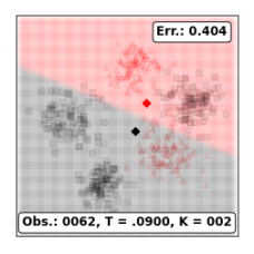
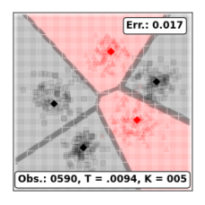
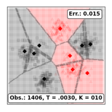
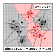
Figure 1: Evolution of the ODA algorithm in 2D binary classification based on class-conditional density estimation. Temperature $T$ decreases from left to right.

Figure 2: Performance curves for the problem of Fig. 1.

Figure 3: Illustration of the evolution of Alg. 1 for binary classification in 2D based on class-conditional density estimation. Showcasing robustness to bad initial conditions which idicates poor local minima prevention.

We first illustrate the properties of Alg. 1, in a classification problem where the data samples were sampled from a mixture of 2D Gaussian distributions. In Fig. 1 and 2, the temperature level (the values of $T$ shown are the normalized values $\lambda=\nicefrac{{1}}{{T+1}}$), the average distortion of the model, the number of codevectors (neurons) used, the number of observations (data samples) used for convergence, as well as the overall time, are shown. Since the objective is to give a geometric illustration of how the algorithm works in the two-dimensional plane, the Euclidean distance is used as the proximity measure. Notice that the classification accuracy for $K=5$ is $98\%$ and it gets to $100\%$ only when we reach $K=144$. This showcases the performance-complexity trade-off that Alg. 1 allows the user to control in an online fashion. Since classification and clustering are handled in a similar way by Alg. 1, these examples properly illustrate the behavior of the proposed methodology for clustering as well.

In Fig. 3, the progression of the learning representation is depicted for a binary classification problem with underlying class distributions shaped as concentric circles. The algorithm starts at high temperature with a single codevector for each class. Here the codevectors are poorly initialized outside the support of the data, which is not assumed known a priori (e.g. online observations of unknown domain). In this example the LVQ algorithm has been shown to fail [40]. This showcases the robustness of the proposed algorithm with respect to the initial configuration. This is an example of poor local minima prevention which, although not theoretically guaranteed, is a known property of annealing optimization methods.

(a) Gaussians.

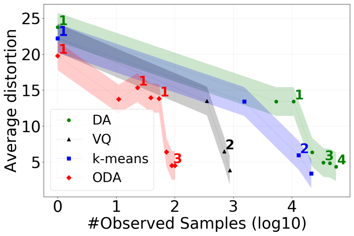
(b) PIMA.

Figure 4: Algorithm comparison for unsupervised learning.

For clustering, we consider the dataset of Fig. 1 (Gaussians), and the PIMA dataset [41]. In Fig. 4, we compare Alg. 1 with the stochastic (online) vector quantization (sVQ) algorithm ([40]), and two offline (batch) algorithms, namely $k$-means [42], and the original deterministic annealing (DA) algorithm [17]. The algorithms are compared in terms of the minimum average distortion achieved, as a function of the number of samples they observed, and the number of clusters they used. The Euclidean distance is used for fair comparison. Since there is no criterion to decide the number of clusters $K$ for $k$-means and sVQ, we run them sequentially for the $K$ values estimated by DA, and add up the computational time. All algorithms are able to achieve comparable average distortion values given good initial conditions and appropriate size $K$. Therefore, the progressive estimation of $K$, as well as the robustness with respect to the initial conditions, are key features of both annealing algorithms. Compared to the offline algorithms, i.e., $k$-means and DA, ODA and sVQ achieve practical convergence with significantly lower number of observations, which corresponds to reduced computational time, as argued above. Compared to the online sVQ (and LVQ), the probabilistic approach of ODA introduces additional computational cost: all neurons are now updated in every iteration, instead of only the winner neuron. However, the updates can still be computed relatively fast when using Bregman divergences (Theorem 3). For more experimental results regarding clustering and classification, the authors are referred to [12, 43, 36].

V-B Reinforcement Learning

Finally, we validate the proposed methodology on the inverted pendulum (Cart-pole) optimal control problem. The state variable of the cart-pole system has four components $(x,\theta,\dot{x},\dot{\theta})$, where $x$ and $\dot{x}$ are the position and velocity of the cart on the track, and $\theta$ and $\dot{\theta}$ are the angle and angular velocity of the pole with the vertical. The cart is free to move within the bounds of a one-dimensional track. The pole is free to move only in the vertical plane of the cart and track.

The action space consists of an impulsive “left” or “right” force $F\in\{-10,+10\}$N of fixed magnitude to the cart at discrete time intervals. The cart-pole system is modeled by the following nonlinear system of differential equations [44]:

$$\ddot{x} =\frac{F+ml\left(\dot{\theta}^{2}\sin\theta-\ddot{\theta}\cos\theta\right)\mu_{c}sgn(\dot{x})}{m_{c}+m}$$

$$\ddot{\theta} =\frac{g\sin\theta+\cos\theta\left(\frac{-F-ml\dot{\theta}^{2}\sin\theta+\mu_{c}sgn(\dot{x})}{m_{c}+m}\right)-\frac{\mu_{p}}{ml}\mu_{c}sgn(\dot{x})}{l\left(\frac{4}{3}-\frac{m\cos^{2}\theta}{m_{c}+m}\right)}$$

where the parameter values for $g,m_{c},m,l,\mu_{c},\mu_{p}$ can be found in [44]. The transition function for the state $x$ is $x_{n+1}=x_{n}+\tau\dot{x}$, where $\tau=0.02$s. The initial state is set to $X_{0}=(u_{x},u_{\theta},u_{\dot{x}},u_{\dot{\theta}})$ where $u_{x}$, $u_{\theta}$, $u_{\dot{x}}$, and $u_{\dot{\theta}}$ follow a uniform distribution $U(-0.05,0.05)$. Failure occurs when $|\theta|>12^{\circ}$ or when $|x|>2.4$m. An episode terminates successfully after $N_{t}$ timesteps, and the average number of timesteps $\hat{N}_{t}\leq N_{t}$ across different attempts, is used to quantify the performance of the learning algorithm. We use the Euclidean distance as the Bregman divergence $d_{\phi}$.

In Fig. 5 we compare the average number of timesteps (here $N_{t}=1000$) with respect to the number of aggregate states used, for three different state aggregation algorithms. The first one is naive discretization without state aggregation, the second is the SOM-based algorithm proposed in [34], and the last is the proposed algorithm Alg. 2. We initialize the codevectors $\mu$ by uniformly discretizing over $\hat{S}\times\left\{-10,10\right\}$, for $\hat{S}=[-1,1]\times[-4,4]\times[-1,1]\times[-4,4]$. We use $K\in\left\{16,81,256,625\right\}$ clusters, corresponding to a standard discretization scheme with only $n\in\left\{2,3,4,5\right\}$ bins for each dimension. As expected, state aggregation outperforms standard discretization of the state-action space. The ability to progressively adapt the number and placement of the centroids of the aggregate states is an important property of the proposed algorithm. Fig. 5 shows $5$ instances of Alg. 2 for $5$ different stopping criteria according to a pre-defined minimum temperature $T_{min}$. This results in different representations of the state space with $K\in\left\{56,118,136,202,252\right\}$ aggregate states, respectively.

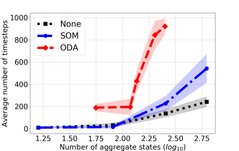
Figure 5: Average number of timesteps ($N_{t}=1000$) over number of aggregate states used. (red) the proposed algorithm. (black) $Q$-learning without state aggregation. (blue) the SOM-based algorithm of [34].

VI Conclusion

We investigate the properties of learning with progressively growing models, and propose an online annealing optimization approach as a learning algorithm that progressively adjusts its complexity with respect to new observations, offering online control over the performance-complexity trade-off. We show that the proposed algorithm constitutes a progressively growing competitive-learning neural network with inherent regularization mechanisms, the learning rule of which is formulated as an online gradient-free stochastic approximation algorithm. The use of stochastic approximation enables the study of the convergence of the learning algorithm through mathematical tools from dynamical systems and control, and allows for its use in supervised, unsupervised, and reinforcement learning settings. In addition, the annealing nature of the algorithm, contributes to poor local minima prevention and offers robustness with respect to the initial conditions. To our knowledge, this is the first time such a progressive approach has been proposed for machine learning and reinforcement learning applications. These results can lead to new developments in the development of progressively growing machine learning models targeted towards applications in which computational resources are limited and robustness and interpretability are prioritized.

Christos N. Mavridis (M’20) received the Diploma degree in electrical and computer engineering from the National Technical University of Athens, Greece, in 2017, and the M.S. and Ph.D. degrees in electrical and computer engineering at the University of Maryland, College Park, MD, USA, in 2021. His research interests include systems and control theory, stochastic optimization, learning theory, multi-agent systems, and robotics. He has served as a postdoctoral associate at the University of Maryland, and a visiting postdoctoral fellow at KTH Royal Institute of Technology, Stockholm. He has worked as a research intern for the Math and Algorithms Research Group at Nokia Bell Labs, NJ, USA, and the System Sciences Lab at Xerox Palo Alto Research Center (PARC), CA, USA. Dr. Mavridis is an IEEE member, and a member of the Institute for Systems Research (ISR) and the Autonomy, Robotics and Cognition (ARC) Lab. He received the Ann G. Wylie Dissertation Fellowship in 2021, and the A. James Clark School of Engineering Distinguished Graduate Fellowship, Outstanding Graduate Research Assistant Award, and Future Faculty Fellowship, in 2017, 2020, and 2021, respectively. He has been a finalist in the Qualcomm Innovation Fellowship US, San Diego, CA, 2018, and he has received the Best Student Paper Award (1st place) in the IEEE International Conference on Intelligent Transportation Systems (ITSC), 2021.

John S. Baras (LF’13) received the Diploma degree in electrical and mechanical engineering from the National Technical University of Athens, Athens, Greece, in 1970, and the M.S. and Ph.D. degrees in applied mathematics from Harvard University, Cambridge, MA, USA, in 1971 and 1973, respectively. He is a Distinguished University Professor and holds the Lockheed Martin Chair in Systems Engineering, with the Department of Electrical and Computer Engineering and the Institute for Systems Research (ISR), at the University of Maryland College Park. From 1985 to 1991, he was the Founding Director of the ISR. Since 1992, he has been the Director of the Maryland Center for Hybrid Networks (HYNET), which he co-founded. His research interests include systems and control, optimization, communication networks, applied mathematics, machine learning, artificial intelligence, signal processing, robotics, computing systems, security, trust, systems biology, healthcare systems, model-based systems engineering. Dr. Baras is a Fellow of IEEE (Life), SIAM, AAAS, NAI, IFAC, AMS, AIAA, Member of the National Academy of Inventors and a Foreign Member of the Royal Swedish Academy of Engineering Sciences. Major honors include the 1980 George Axelby Award from the IEEE Control Systems Society, the 2006 Leonard Abraham Prize from the IEEE Communications Society, the 2017 IEEE Simon Ramo Medal, the 2017 AACC Richard E. Bellman Control Heritage Award, the 2018 AIAA Aerospace Communications Award. In 2016 he was inducted in the A. J. Clark School of Engineering Innovation Hall of Fame. In 2018 he was awarded a Doctorate Honoris Causa by his alma mater the National Technical University of Athens, Greece.

References

- [1] K. P. Bennett and E. Parrado-Hernández, “The interplay of optimization and machine learning research,” The Journal of Machine Learning Research, vol. 7, pp. 1265–1281, 2006.
- [2] Y. LeCun, Y. Bengio, and G. Hinton, “Deep learning,” nature, vol. 521, no. 7553, pp. 436–444, 2015.
- [3] N. C. Thompson, K. Greenewald, K. Lee, and G. F. Manso, “The computational limits of deep learning,” arXiv preprint arXiv:2007.05558, 2020.
- [4] E. Strubell, A. Ganesh, and A. McCallum, “Energy and policy considerations for deep learning in nlp,” arXiv preprint arXiv:1906.02243, 2019.
- [5] C. Szegedy, W. Zaremba, I. Sutskever, J. Bruna, D. Erhan, I. Goodfellow, and R. Fergus, “Intriguing properties of neural networks,” arXiv preprint arXiv:1312.6199, 2013.
- [6] N. Carlini and D. Wagner, “Towards evaluating the robustness of neural networks,” in 2017 ieee symposium on security and privacy (sp). IEEE, 2017, pp. 39–57.
- [7] V. Sehwag, A. N. Bhagoji, L. Song, C. Sitawarin, D. Cullina, M. Chiang, and P. Mittal, “Analyzing the robustness of open-world machine learning,” in Proceedings of the 12th ACM Workshop on Artificial Intelligence and Security, 2019, pp. 105–116.
- [8] H. Xu and S. Mannor, “Robustness and generalization,” Machine learning, vol. 86, no. 3, pp. 391–423, 2012.
- [9] C. G. Northcutt, A. Athalye, and J. Mueller, “Pervasive label errors in test sets destabilize machine learning benchmarks,” arXiv preprint arXiv:2103.14749, 2021.
- [10] A. Raghunathan, S. M. Xie, F. Yang, J. C. Duchi, and P. Liang, “Adversarial training can hurt generalization,” arXiv preprint arXiv:1906.06032, 2019.
- [11] C. N. Mavridis and J. S. Baras, “Convergence of stochastic vector quantization and learning vector quantization with bregman divergences,” IFAC-PapersOnLine, vol. 53, no. 2, 2020.
- [12] ——, “Online deterministic annealing for classification and clustering,” IEEE Transactions on Neural Networks and Learning Systems, 2022.
- [13] M. Biehl, B. Hammer, and T. Villmann, “Prototype-based models in machine learning,” Wiley Interdisciplinary Reviews: Cognitive Science, vol. 7, no. 2, pp. 92–111, 2016.
- [14] C. Mavridis, E. Noorani, and J. S. Baras, “Risk sensitivity and entropy regularization in prototype-based learning,” in 2022 30th Mediterranean Conference on Control and Automation (MED). IEEE, 2022, pp. 194–199.
- [15] E. A. Uriarte and F. D. Martín, “Topology preservation in som,” International journal of applied mathematics and computer sciences, vol. 1, no. 1, pp. 19–22, 2005.
- [16] S. Saralajew, L. Holdijk, M. Rees, and T. Villmann, “Robustness of generalized learning vector quantization models against adversarial attacks,” in International Workshop on Self-Organizing Maps. Springer, 2019, pp. 189–199.
- [17] K. Rose, “Deterministic annealing for clustering, compression, classification, regression, and related optimization problems,” Proceedings of the IEEE, vol. 86, no. 11, pp. 2210–2239, 1998.
- [18] G. E. Hinton, S. Osindero, and Y.-W. Teh, “A fast learning algorithm for deep belief nets,” Neural computation, vol. 18, no. 7, pp. 1527–1554, 2006.
- [19] H. Robbins and S. Monro, “A stochastic approximation method,” The annals of mathematical statistics, pp. 400–407, 1951.
- [20] V. S. Borkar, Stochastic approximation: a dynamical systems viewpoint. Springer, 2009, vol. 48.
- [21] A. Banerjee, S. Merugu, I. S. Dhillon, and J. Ghosh, “Clustering with bregman divergences,” Journal of machine learning research, vol. 6, no. Oct, pp. 1705–1749, 2005.
- [22] T. Villmann, S. Haase, F.-M. Schleif, B. Hammer, and M. Biehl, “The mathematics of divergence based online learning in vector quantization,” in IAPR Workshop on Artificial Neural Networks in Pattern Recognition. Springer, 2010, pp. 108–119.
- [23] D. E. Rumelhart, G. E. Hinton, and R. J. Williams, “Learning representations by back-propagating errors,” nature, vol. 323, no. 6088, pp. 533–536, 1986.
- [24] L. Bottou, “Online learning and stochastic approximations,” On-line learning in neural networks, vol. 17, no. 9, p. 142, 1998.
- [25] C. J. Watkins and P. Dayan, “Q-learning,” Machine learning, vol. 8, no. 3-4, pp. 279–292, 1992.
- [26] J. N. Tsitsiklis, “Asynchronous stochastic approximation and q-learning,” Machine learning, vol. 16, no. 3, pp. 185–202, 1994.
- [27] V. S. Borkar and S. P. Meyn, “The ode method for convergence of stochastic approximation and reinforcement learning,” SIAM Journal on Control and Optimization, vol. 38, no. 2, pp. 447–469, 2000.
- [28] V. S. Borkar, “Stochastic approximation with two time scales,” Systems & Control Letters, vol. 29, no. 5, pp. 291–294, 1997.
- [29] T. Kohonen, Learning Vector Quantization. Berlin, Heidelberg: Springer Berlin Heidelberg, 1995, pp. 175–189.
- [30] E. T. Jaynes, “Information theory and statistical mechanics,” Physical review, vol. 106, no. 4, p. 620, 1957.
- [31] T. D. Hocking, A. Joulin, F. Bach, and J.-P. Vert, “Clusterpath an algorithm for clustering using convex fusion penalties,” in 28th international conference on machine learning, 2011, p. 1.
- [32] L. Devroye, L. Györfi, and G. Lugosi, A probabilistic theory of pattern recognition. Springer Science & Business Media, 2013, vol. 31.
- [33] A. Sato and K. Yamada, “Generalized learning vector quantization,” in Advances in neural information processing systems, 1996, pp. 423–429.
- [34] C. N. Mavridis and J. S. Baras, “Vector quantization for adaptive state aggregation in reinforcement learning,” in 2021 American Control Conference (ACC). IEEE, 2021, pp. 2187–2192.
- [35] C. N. Mavridis, N. Suriyarachchi, and J. S. Baras, “Maximum-entropy progressive state aggregation for reinforcement learning,” in 2021 60th IEEE Conference on Decision and Control (CDC). IEEE, 2021, pp. 5144–5149.
- [36] C. N. Mavridis, G. Kontoudis, and J. S. Baras, “Sparse gaussian process regression using progressively growing learning representations,” in 2022 61st IEEE Conference on Decision and Control (CDC). IEEE, 2022.
- [37] T. Haarnoja, H. Tang, P. Abbeel, and S. Levine, “Reinforcement Learning with Deep Energy-Based Policies,” in Proceedings of the 34th International Conference on Machine Learning - Volume 70, ser. ICML’17. JMLR.org, 2017, p. 1352–1361.
- [38] J. Schulman, F. Wolski, P. Dhariwal, A. Radford, and O. Klimov, “Proximal Policy Optimization Algorithms,” arXiv preprint arXiv:1707.06347, 2017.
- [39] E. Noorani, C. Mavridis, and J. Baras, “Risk-sensitive reinforcement learning with exponential criteria,” arXiv, 2022.
- [40] J. S. Baras and A. LaVigna, “Convergence of a neural network classifier,” in Advances in Neural Information Processing Systems, 1991, pp. 839–845.
- [41] J. W. Smith, J. Everhart, W. Dickson, W. Knowler, and R. Johannes, “Using the adap learning algorithm to forecast the onset of diabetes mellitus,” in Proceedings of the annual symposium on computer application in medical care. American Medical Informatics Association, 1988, p. 261.
- [42] L. Bottou and Y. Bengio, “Convergence properties of the k-means algorithms,” in Advances in neural information processing systems, 1995, pp. 585–592.
- [43] C. N. Mavridis and J. S. Baras, “Progressive graph partitioning based on information diffusion,” in 2021 60th IEEE Conference on Decision and Control (CDC). IEEE, 2021, pp. 37–42.
- [44] A. G. Barto, R. S. Sutton, and C. W. Anderson, “Neuronlike adaptive elements that can solve difficult learning control problems,” IEEE transactions on systems, man, and cybernetics, no. 5, pp. 834–846, 1983.