A geometric framework for asymptotic inference of principal subspaces in PCA

Abstract

In this article, we develop an asymptotic method for testing hypothesis on the set of all linear subspaces arising from PCA and for constructing confidence regions for this set. This procedure is derived from intrinsic estimation in each Grassmannian, endowed with a structure of Riemannian manifold, to which each of these subspaces belong.

1 Introduction

Let $X$ be Gaussian a random vector valued in $\mathbb{R}^{d}$, $d\geq 1$, with covariance matrix $\Sigma$. Denote by $\lambda_{1}>...>\lambda_{r}$ the different eigenvalues of $\Sigma$ and by $\mathrm{I}=(q_{i})_{1\leq i\leq r}$ their respective multiplicities. The sequence $\mathrm{I}$ induces a partition of the indices $(1,...,d)$ into $r$ parts $(B_{i})_{1\leq i\leq r}$, of respective sizes $(q_{i})_{1\leq i\leq r}$. For example, $B_{1}=(1,...,q_{1})$ and $B_{r}=(q_{r-1}+1,...,d)$. In PCA, the principal subspaces (PS’s) are defined as the eigenspaces of $\Sigma$, denoted by $\left(P_{i}(\Sigma)\right)_{1\leq i\leq r}$. Now, $\Sigma$ is estimated by the sample covariance matrices $(\widehat{\Sigma}_{n})_{n\geq 1}$ from iid samples of $X$. Recall that almost surely, for all $n\geq 1$, $\widehat{\Sigma}_{n}$ has $d$ distinct (random) eigenvalues $\mu_{1}\left(\widehat{\Sigma}_{n}\right)>...>\mu_{d}\left(\widehat{\Sigma}_{n}\right)$. To estimate the eigenspaces of $\Sigma$, these eigenvalues need to be regrouped according to the sequence $\mathrm{I}$: the PS’s are estimated by the eigenspaces $\left(P_{i}\left(\widehat{\Sigma}_{n}\right)\right)_{1\leq i\leq r}$ which are the linear subspaces spanned by the eigenvectors of $\widehat{\Sigma}_{n}$ associated to its eigenvalues in $M_{n}^{i}:=\left\{\mu_{k}\left(\widehat{\Sigma}_{n}\right):k\in B_{i}\right\}$.

The landmark papers Anderson 1963 (Anderson, 1963) and Tyler 1981 (Tyler, 1981) investigated the inference of a single PS from the asymptotic distribution of statistics involving the eigenvectors of $\widehat{\Sigma}_{n}$. The inference obtained for a PS of dimension $q=1$ in Anderson 1963 (Anderson, 1963) was generalized to the case of one PS of any dimension $q\geq 1$ in Tyler 1981 (Tyler, 1981) using linear algebraic methods. In contrast, we introduce in this paper a geometric setting which allow us to derive the inference of all PS’s together, for any sequence of dimensions. Namely, a given PS belongs to a Grassmannian, while the collection $F^{\mathrm{I}}(\Sigma):=\left(P_{i}(\Sigma)\right)_{1\leq i\leq r}$ of them lies in a Flag manifold. Here, a flag is viewed as a collection $\mathcal{P}=\left(P_{i}\right)_{1\leq i\leq r}$ of mutually orthogonal subspaces spanning $\mathbb{R}^{d}$, indexed by its type, that is the sequence $\mathrm{I}=(q_{i})_{1\leq i\leq r}$ of dimensions of the $P_{i}$’s. This incremental subspaces representation is equivalent to the more classical one as properly nested sequence of linear subspaces. We denote by $\mathcal{F}^{\mathrm{I}}$ the set of all flags of type $\mathrm{I}$. In order to estimate the PS’s, the idea is then to endow Grassmannians and flags of given type with a structure of Riemannian manifold, allowing to perform intrinsic estimation, based on Central Limit Theorems (CLT’s), as in Bhattacharya and Patrangenaru 2005 (Bhattacharya and Patrangenaru, 2005). It is well-known that $\mathcal{F}^{\mathrm{I}}$ is diffeomorphic to $O(d)/O(\mathrm{I})$, where $O(d)$ is the orthogonal group of $\mathbb{R}^{d}$ and $O(\mathrm{I}):=O(q_{1})\times...\times O(q_{r})$. While in Tyler 1981 (Tyler, 1981) each PS is estimated separately, our geometric approach enables us to estimate the whole flag $F^{\mathrm{I}}(\Sigma)$ from the limiting distribution of the sample flag $F^{\mathrm{I}}(\widehat{\Sigma}_{n}):=\left(P_{i}(\widehat{\Sigma}_{n})\right)_{1\leq i\leq r}$.

In order to obtain Confidence Regions for $F^{\mathrm{I}}(\Sigma)$ in $\mathcal{F}^{\mathrm{I}}$, a first method could be to establish a CLT in $\mathcal{F}^{\mathrm{I}}$ in normal coordinates, following Bhattacharya and Patrangenaru 2005 (Bhattacharya and Patrangenaru, 2005). However, the Riemannian Logarithm and even the geodesic distance are unknown in closed form in $\mathcal{F}^{\mathrm{I}}$. The representation of a flag by its incremental subspaces is a key point of our method: it allows embedding the flag space $\mathcal{F}^{\mathrm{I}}$ in the product of Grassmanians $\mathrm{G}^{\mathrm{I}}$, for which the geometry is much simpler and the Logarithm is available in closed form. We establish CLT’s in Grassmannians for each $P_{i}(\widehat{\Sigma}_{n})$ and we prove that their rate of convergence to a Gaussian distribution are of order $\frac{1}{\sqrt{n}}$. Thanks to the fact that the tangent space to all Grassmanians can be embedded in the same symmetric matrix space with the projector representation, we then derive the estimation of the whole flag $F^{\mathrm{I}}(\Sigma)$. Namely, we prove a result of the form

$$n\Delta_{\mbox{Spec}(\Sigma)}\left(F^{\mathrm{I}}\left(\Sigma\right),F^{\mathrm{I}}\left(\widehat{\Sigma}_{n}\right)\right)\xrightarrow[n\rightarrow\infty]{d}\chi^{2}_{D},$$ (1.1)

for some $D>0$. Here, $\Delta_{\mbox{Spec}(\Sigma)}\left(\cdot,\cdot\right)$ can be viewed as a discrepancy function on $\mathcal{F}^{\mathrm{I}}$, indexed by the spectrum of $\Sigma$. The convergence in $(\ref{mainCV})$ is proved rigorously and checked numerically on synthetic experiments. In an estimation setting, the unknown eigenvalues of $\Sigma$ are replaced by the block-means of eigenvalues of the empirical matrix $\widehat{\Sigma}_{n}$. Thanks to the consistency of this estimator, the convergence to the $\chi^{2}_{D}$ distribution is preserved, and this provides confidence regions for $F^{\mathrm{I}}\left(\Sigma\right)$.

This article is organized as follows. In Section 2, we develop the background of geometry of Grassmannians and Flag manifolds needed for the asymptotic inference methods derived in Section 3.

2 Grassmannian and Flags

For Riemannian manifolds, we refer to Lee 2018 (Lee, 1963). Our reference for the geometry of Grassmannians is Bendokat Zimmermann and Absil 2020 (Bendokat Zimmermann and Absil, 2020) and for that of Flag manifolds is Ye Wong and Lim 2022 (Ye Wong and Lim, 2022). The key formula for the closed form for the Riemannian Logarithm for Grassmannians (Theorem 1 below) is due to Batzies Huper Machado and Silva Leite 2015 (Batzies Huper Machado and Silva Leite, 2015).

2.1 The Grassmannian manifold

For $1\leq q<d$, the Grassmannian $G(q,d)$ is by definition the set of all linear subspaces of dimension $q$ of $\mathbb{R}^{d}$. In order to perform calculations, it is identified with the set of orthogonal projectors of rank $q$:

$$G(q,d)\simeq\left\{P\in\mathbb{R}^{d\times d}:P^{\prime}=P,\leavevmode\nobreak\ P^{2}=P,\leavevmode\nobreak\ \textrm{rank}(P)=q\right\}.$$ (2.1)

Then, we introduce the Stiefel manifold $\mathrm{St(q,d)}$. As a set, it is the set of all $d\times q$ matrices whose columns are orthonormal vectors. Denoting by $I_{d}$ the identity matrix of order $d$,

$$\mathrm{St(q,d)}=\left\{Y\in\mathbb{R}^{d\times q}:Y^{\prime}Y=I_{d}\right\}.$$

The sets $G(q,d)$ and $\mathrm{St(q,d)}$ are linked by the map $\pi_{q}^{SG}:St(q,d)\longrightarrow G(q,d)$, which associates to any set of $q$ orthonormal vectors, the projector whose range is the subspace which they span, i.e.:

$$\pi_{q}^{SG}(Y)=YY^{\prime}.$$

2.1.1 Action of the orthogonal group

The orthogonal group $O(d)$ acts on $G(q,d)$ by

$$(Q,P)\longmapsto QPQ^{\prime},\quad\textrm{for }Q\in O(d)\textrm{ and }P\in G(q,d).$$ (2.2)

Let $P_{0}\in G(q,d)$ whose range is spanned by the $q$ first vectors of the standard basis of $\mathbb{R}^{d}$. Let $\pi_{q}^{OG}$ be the map defined by

$$\pi_{q}^{OG}:O(d)\longrightarrow G(q,d)\quad,\quad\pi_{q}^{OG}(Q)=QP_{0}Q^{\prime}.$$

Fix $P\in G(q,d)$. Then, for any $Q\in O(d)$ whose $q$ first columns span the range of $P$, we have that $\pi_{q}^{OG}(Q)=P$. So, the orbit of $P_{0}$ is the whole $G(q,d)$. On the other hand, the stabilizer of $P_{0}$ is identified with $O(q)\times O(d-q)$, so that $\pi_{q}^{OG}$ induces a bijection

$$\widetilde{\pi}_{q}^{OG}:O(d)/(O(q)\times O(d-q))\simeq G(q,d).$$

Now, $O(d)/(O(q)\times O(d-q))$ is endowed with the manifold structure such that the canonical quotient map from $O(d)$ to $O(d)/(O(q)\times O(d-q))$ is a smooth submersion, i.e. with surjective differential at every point. Then, the manifold structure on $G(q,d)$ is the one for which $\widetilde{\pi}_{q}^{OG}$ is a diffeomorphism.

2.1.2 Tangent space

By definition, the Lie algebra of $O(d)$ is the tangent space $T_{I_{d}}O(d)$. It is the set $\mathfrak{so}(d)$ of skew-symmetric matrices. Now, for any $Q\in O(d)$,

$$T_{Q}O(d)=\left\{Q\widetilde{\Omega}:\widetilde{\Omega}\in\mathfrak{so}(d)\right\}.$$

Then, the tangent space at $P\in G(q,d)$ is the linear subspace of $\mathrm{Sym}_{d}$ defined by

$$T_{P}G(q,d)=\left\{\Delta\in\mathrm{Sym}_{d}:\Delta P+P\Delta=\Delta\right\}.$$

2.2 Riemmannian geometry of the Grassmannian

2.2.1 Metric

A metric on a smooth manifold $M$ is a collection $g=(g_{p})_{p\in M}$ of inner products on the tangent spaces $T_{p}M$, varying smoothly wrt $p$. We say that $(M,g)$ is a Riemannian manifold and we assume in the sequel that $M$ is connected. For $v\in T_{p}M$, its length is $\left\|v\right\|_{p}:=\left(g_{p}(v,v)\right)^{1/2}$ . For $p,q\in M$, a $C^{1}$ curve between $p$ and $q$ is a $C^{1}$ map $\gamma:[a,b]\longrightarrow M$ such that $\gamma(a)=p$ and $\gamma(b)=q$. Its length is $\int_{a}^{b}\left\|\frac{d}{dt}\gamma(t)\right\|_{\gamma(t)}dt$. Then, $g$ defines the geodesic distance $d_{g}$, where for any $p,q\in M$, $d_{g}(p,q)$ is the infimum of lengths of all $C^{1}$ curves between $p$ and $q$.

Let $\pi:M\longrightarrow N$ be a smooth submersion. A metric $g$ on $M$ allows to split any tangent space $T_{p}M$ into a vertical part $\mathrm{Ver}_{p}^{\pi}M:=\mathrm{ker}(d\pi_{p})$ and a horizontal part $\mathrm{Hor}_{p}^{\pi}M$, which is the orthogonal complement of $\mathrm{Ver}_{p}^{\pi}M$ in $T_{p}M$ wrt $g_{p}$. We say that $\pi$ is a Riemannian submersion when, for all $p\in M$, the restriction of $d\pi_{p}$ to $\mathrm{Hor}_{p}^{\pi}M$ is an isometry.

As a compact Lie group, $O(d)$ is endowed with its canonical metric $g^{O}$ defined by

$$g_{Q}^{O}(\Omega_{1},\Omega_{2})=\frac{1}{2}\mathrm{tr}(\Omega_{1}^{\prime}\Omega_{2}),\quad\textrm{for }Q\in O(d),\leavevmode\nobreak\ \Omega_{i}\in T_{Q}O(d).$$

We endow $G(q,d)$ with the unique metric $g^{G}$ for which $\pi^{OG}$ is a Riemannian submersion. Thus, for $P\in G(q,d)$ and $\Delta_{1},\Delta_{2}\in T_{P}G(q,d)$,

$$g_{P}^{G}(\Delta_{1},\Delta_{2})=g_{Q}^{O}(\Delta_{1,Q}^{h},\Delta_{2,Q}^{h})$$

where $\Delta_{i,Q}^{h}$ is the horizontal lift at $Q$ of $\Delta_{i}$, i.e. $\Delta_{i,Q}^{h}\in\mathrm{Hor}_{Q}O(d)$ and $d\pi^{OG}_{Q}\left(\Delta_{i,Q}^{h}\right)=\Delta_{i}$.

Lemma 1.

The action of $O(d)$ on $G(q,d)$ defined above is an isometry. This means that, for any $P,R\in G(q,d)$ and $Q\in O(d)$,

$$d_{g}^{G}\left(QPQ^{\prime},QRQ^{\prime}\right)=d_{g}^{G}\left(P,R\right),$$

where $d_{g}^{G}$ denotes the geodesic distance on $G(q,d)$ associated to $g^{G}$.

2.2.2 Geodesics

Let $\gamma$ be a smooth curve in $M$. If $M$ is a submanifold of $\mathbb{R}^{n}$, then the acceleration $\ddot{\gamma}(t)$ is not always a tangent vector at $\gamma(t)$. On a Riemannian manifold $(M,g)$, one builds from the metric an operation of derivation of vector fields whose outputs are tangent vectors, called the covariant derivative and denoted by $\nabla$. Thus, if $\gamma$ is in $(M,g)$, the acceleration vector of $\gamma$ at $\gamma(t)$ is the vector of $T_{\gamma(t)}M$ equals to the covariant derivative of the velocity $\dot{\gamma}$ at $\gamma(t)$ in the direction of $\dot{\gamma}(t)$, denoted by $\left(\nabla_{\dot{\gamma}}\dot{\gamma}\right)_{\gamma(t)}$. Then, a geodesic is a smooth curve $\gamma$ on $M$ of zero acceleration, i.e. such that

$$\nabla_{\dot{\gamma}}\dot{\gamma}=0.$$

This equation is locally an ODE, so that for any $p\in M$ and $v\in T_{p}M$, there exists a unique geodesic $\gamma_{p,v}$ such that $\gamma_{p,v}(0)=p$ and $\dot{\gamma_{p,v}}(0)=v$. By the Hopf-Rinow theorem, the metric space $(M,d_{g})$ is complete if and only if all geodesics are defined on $\mathbb{R}$. In that case, for any $p,q\in M$, there exists at least one geodesic of minimal length between $p$ and $q$. Given a Riemannian submersion $\pi:M\longrightarrow N$, the geodesics in $N$ are the images by $\pi$ of the geodesics with horizontal tangent vectors in $M$. Since $\pi^{OG}$ is a Riemannian submersion, the geodesics in $G(q,d)$ are given by those in $O(d)$. The geodesic in $O(d)$ starting at $Q$ with initial velocity $Q\widetilde{\Omega}$ is

$$t\longmapsto Q\exp_{m}(t\widetilde{\Omega}),$$

where $\exp_{m}$ is the matrix exponential. So, the geodesic in $G(q,d)$ starting at $P$ with initial velocity $\Delta$ is

$$t\longmapsto\pi^{OG}\left(Q\exp_{m}(t\widetilde{\Omega})\right)=Q\exp_{m}(t\widetilde{\Omega})P_{0}\exp_{m}(-t\widetilde{\Omega})Q^{\prime},$$ (2.3)

for any $Q\in\left(\pi^{OG}\right)^{-1}\left(P\right)$ and where $Q\widetilde{\Omega}=\Delta_{Q}^{h}$. Therefore, $\left(G(q,d),g^{O}\right)$ is complete.

2.2.3 Exponential map

In the sequel, $(M,g)$ is a complete Riemannian manifold. For any $p\in M$, the Riemannian exponential at $p$ is the map $\mathrm{Exp}_{p}^{M}$ from $T_{p}M$ to $M$ defined by

$$\mathrm{Exp}_{p}^{M}(v)=\gamma_{p,v}(1).$$

Lemma 2.

By $(\ref{geodesicGrass})$, for any $P\in G(q,d)$ and $\Delta\in T_{P}G(q,d)$,

$$\mathrm{Exp}_{P}^{G(q,d)}(\Delta)=\exp_{m}([\Delta,P])P\exp_{m}(-[\Delta,P]).$$

2.2.4 Cut locus

It is known that, for all $p\in M$, any geodesic starting at $p$ is locally length-minimizing. The cut locus of $p\in M$ is the set $\mathrm{Cut}(p)$ of points $q$ such that the geodesics starting at $p$ cease to be length-minimizing beyond $q$. It is established that if $q\notin\mathrm{Cut}(p)$, then there exists a unique length-minimizing geodesic between $p$ and $q$. For exemple, on a sphere, the geodesics are the great circles, so that two antipodal points are each other’s cut locus.

Lemma 3.

Let $P\in G(q,d)$. Then, writing $P=YY^{\prime}$,

$$\mathrm{Cut}(P)=\left\{R=ZZ^{\prime}\in G(q,d):\mathrm{rank}\left(Y^{\prime}Z\right)<q\right\}.$$

This means that this characterization is independent of $Y\in\mathrm{St}(q,d)$ such that $P=YY^{\prime}$.

2.2.5 Riemannian Logarithm

Let $p\in M$ and $q\in M\setminus\mathrm{Cut}(p)$. Then, there exists a unique shortest geodesic between $p$ and $q$, whose initial velocity is thus the smallest tangent vector $v\in T_{p}M$ such that $\mathrm{Exp}_{p}^{M}\left(v\right)=q$. It is called the Riemannian Logarithm of $q$ at $p$, denoted by $\mathrm{Log}_{p}^{M}(q)$. We have that

$$d_{g}(p,q)=\left\|\mathrm{Log}_{p}^{M}(q)\right\|_{p}.$$ (2.4)

For $G(q,d)$, combining $(\ref{dgLog})$, Lemmas 3 and 1 yield the following result.

Proposition 1.

For all $P,R\in G(q,d)$ and $Q\in O(d)$,

$$QRQ^{\prime}\notin\mathrm{Cut}(QPQ^{\prime})\iff R\notin\mathrm{Cut}(P),$$ (2.5)

and in that case,

$$\left\|\mathrm{Log}_{QPQ^{\prime}}^{G(q,d)}\left(QRQ^{\prime}\right)\right\|_{QPQ^{\prime}}=\left\|\mathrm{Log}_{P}^{G(q,d)}\left(R\right)\right\|_{P}.$$ (2.6)

Finally, the next result provides the closed form for the Riemannian Logarithm for $G(q,d)$.

Theorem 1.

Let $P\in G(q,d)$ and $R\in G(q,d)\setminus\mathrm{Cut}(P)$. Then, $\mathrm{Log}_{P}^{G(q,d)}(R)=[\Omega,P]$, where $\Omega$ is determined by

$$\Omega=\frac{1}{2}\log_{m}\left((I_{d}-2R)(I_{d}-2P)\right),$$

and $\log_{m}$ denotes the matrix logarithm.

2.3 The set of flags of fixed type

Let $\mathrm{I}=(q_{i})_{1\leq i\leq r}$ be a sequence of positive integers such that $\sum\limits_{i=1}^{r}q_{i}=d$.

2.3.1 Notations

The sequence $\mathrm{I}$ induces a partition of the indices $\left\{1,...,d\right\}$ into $r$ parts $(B_{i})_{1\leq i\leq r}$, i.e. $B_{1}=(1,...,q_{1})$, $B_{r}=(q_{r-1}+1,...,d)$ and for $1<i<r$, $B_{i}=(\overline{q}_{i-1}+1,...,\overline{q}_{i})$, where $\overline{q}_{i}:=\sum\limits_{j=1}^{i}q_{j}$. Let $A$ be a $d\times d$ matrix. If $A$ is defined by its columns, i.e. $A=[A_{1},...,A_{d}]$, then, for all $1\leq i\leq r$, set

$$A^{(i)}:=[A_{k}:k\in B_{i}].$$

If $A$ is defined by its entries, i.e. $A=(a_{k\ell})_{1\leq k\leq\ell\leq d}$, then, for all $1\leq i\leq j\leq r$, set

$$A^{(ij)}:=(a_{k\ell})_{\begin{subarray}{c}k\in B_{i}\\ \ell\in B_{j}\end{subarray}}.$$

Then, setting $I_{d}^{(i)}:=\left(I_{d}\right)^{(i)}$, we have that $A^{(i)}=AI_{d}^{(i)}$ and $A^{(ij)}=\left(I_{d}^{(i)}\right)^{\prime}AI_{d}^{(j)}$.

2.3.2 Definitions

We recall that a flag of type $\mathrm{I}$ is a collection $\mathcal{V}=(V_{i})_{1\leq i\leq r}$ of $r$ mutually orthogonal linear subspaces of $\mathbb{R}^{d}$ such that for all $1\leq i\leq r$, $\dim(V_{i})=q_{i}$. Thus, the set $\mathcal{F}^{\mathrm{I}}$ of flags of type $\mathrm{I}$ is a subset of

$$\mathrm{G}^{\mathrm{I}}:=\prod\limits_{i=1}^{r}G^{i}\quad\textrm{where}\quad G^{i}:=G(q_{i},d).$$

Identifying Grassmannians with projectors as in $(\ref{identifyGrass})$,

$$\mathcal{F}^{\mathrm{I}}\simeq\left\{\mathcal{P}=(P_{i})_{1\leq i\leq r}\in\mathrm{G}^{\mathrm{I}}:P_{i}P_{j}=0,i\neq j\right\}.$$

Introduce the standard flag $\mathcal{P}_{0}^{\mathrm{I}}=(P_{0}^{i})_{1\leq i\leq r}$, where $P_{0}^{i}\in G^{i}$ is the block-diagonal matrix defined by

$$P_{0}^{i}:=\mathrm{Diag}[0_{q_{1}},...,I_{q_{i}},...,0_{q_{r}}],$$

and $0_{q_{i}}$ is the null matrix of order $q_{i}$. Then,

$$P_{0}^{i}=I_{d}^{(i)}\left(I_{d}^{(i)}\right)^{\prime}.$$ (2.7)

2.3.3 Action of the orthogonal group

The action of $O(d)$ on Grassmanianns induces an action of $O(d)$ on $\mathcal{F}^{\mathrm{I}}$, defined by

$$(Q,\mathcal{P})\mapsto(QP_{i}Q^{\prime})_{1\leq i\leq r}\in\mathcal{F}^{\mathrm{I}},$$

for $Q\in O(d)$ and $\mathcal{P}=(P_{i})_{1\leq i\leq r}\in\mathcal{F}^{\mathrm{I}}$. Indeed, $O(d)$ acts naturally on $\mathrm{G}^{\mathrm{I}}$ and this action preserves the mutual orthogonality of linear subspaces. Then, define the map $\pi^{\mathrm{I}}:O(d)\longrightarrow\mathcal{F}^{\mathrm{I}}$ by

$$\pi^{\mathrm{I}}(Q)=(QP_{0}^{i}Q^{\prime})_{1\leq i\leq r}.$$

Proposition 2.

The orbit of $\mathcal{P}_{0}^{\mathrm{I}}$ under this action is the whole $\mathcal{F}^{\mathrm{I}}$ and the stabilizer of $\mathcal{P}_{0}^{\mathrm{I}}$ is the group $O(\mathrm{I})$, where

$$O(\mathrm{I}):=\left\{\mathrm{Diag}[H_{1},...,H_{r}]:H_{i}\in O(q_{i}),1\leq i\leq r\right\}=\prod\limits_{i=1}^{r}O(q_{i}).$$

In other words, the map $\pi^{\mathrm{I}}$ is surjective and for all $Q\in O(d)$ and $H\in O(\mathrm{I})$, $\pi^{\mathrm{I}}(QH)=\pi^{\mathrm{I}}(Q)$. Therefore, $\pi^{\mathrm{I}}$ induces a bijection

$$\widetilde{\pi}^{\mathrm{I}}:O(d)/O(\mathrm{I})\simeq\mathcal{F}^{\mathrm{I}}.$$

such that $\pi^{\mathrm{I}}=\widetilde{\pi}^{\mathrm{I}}\circ\overline{p}^{\mathrm{I}}$, where $\overline{p}^{\mathrm{I}}$ is the canonical quotient map from $O(d)$ to $O(d)/O(\mathrm{I})$.

Now, let $\pi_{\mathrm{I}}^{SG}$ be the map from $\mathrm{St}^{\mathrm{I}}:=\prod\limits_{i=1}^{r}\mathrm{St}(q_{i},d)$ to $\mathrm{G}^{\mathrm{I}}$ defined by

$$\mathcal{Y}=(Y_{i})_{1\leq i\leq r}\longmapsto\left(\pi_{q_{i}}^{SG}(Y_{i})\right)_{1\leq i\leq r}.$$

Set $\mathrm{St}^{\mathrm{I}}_{\perp}=\left\{\mathcal{Y}=\left(Y_{i}\right)_{1\leq i\leq r}\in\mathrm{St}^{\mathrm{I}}:(Y_{i})^{\prime}Y_{j}=0,i\neq j\right\}$. Then, the restriction of $\pi_{\mathrm{I}}^{SG}$ to $\mathrm{St}^{\mathrm{I}}_{\perp}$ is valued in $\mathcal{F}^{\mathrm{I}}$.

Lemma 4.

Let $\pi_{\mathrm{I}}^{OS}$ be the bijection between $O(d)$ and $\mathrm{St}^{\mathrm{I}}_{\perp}$ defined by $\pi_{\mathrm{I}}^{OS}\left(Q\right)=\left(Q^{(i)}\right)_{1\leq i\leq r}$. Then, for all $Q\in O(d)$,

$$\pi_{\mathrm{I}}^{SG}\left(\pi_{\mathrm{I}}^{OS}\left(Q\right)\right)=\pi^{\mathrm{I}}(Q).$$

Proof.

For $Q\in O(d)$, $\pi_{\mathrm{I}}^{SG}\left(\pi_{\mathrm{I}}^{OS}\left(Q\right)\right)=\left(\pi_{q_{i}}^{SG}(Q^{(i)})\right)_{1\leq i\leq r}$ and for all $1\leq i\leq r$, by $(\ref{PzeroId})$,

$$\pi_{q_{i}}^{SG}\left(Q^{(i)}\right)=Q^{(i)}\left(Q^{(i)}\right)^{\prime}=\left(QI_{d}^{(i)}\right)\left(QI_{d}^{(i)}\right)^{\prime}=QP_{0}^{i}Q^{\prime}.$$

∎

Corollary 1.

The triangles of the following diagram commute.

2.4 Flag of eigenspaces

For $S\in\mathrm{Sym}_{d}$, its spectrum is denoted by

$$\mathrm{Spec}(S)=\left\{\mu_{1}(S)\geq...\geq\mu_{d}(S)\right\}.$$

We denote by $\mathrm{Sym}_{d}^{\neq}$ the set of $S\in\mathrm{Sym}_{d}$ such that $\mu_{1}(S)>...>\mu_{d}(S)$. For all $1\leq i\leq r$, set $\overline{q}_{i}:=\sum\limits_{j=1}^{i}q_{j}$. Let $\overline{\mathrm{Sym}}_{d}^{(\mathrm{I})}$ be the set of $S\in\mathrm{Sym}_{d}$ such that for all $1\leq i\leq r-1$, $\mu_{\overline{q}_{i}}(S)>\mu_{\overline{q}_{i}+1}(S)$. Denote by $\mathrm{Sym}_{d}^{\mathrm{I}}$ the set of $S\in\overline{\mathrm{Sym}}_{d}^{(\mathrm{I})}$ such that for all $1\leq i\leq r$ and $k,\ell$ in $B^{i}$, $\mu_{k}(S)=\mu_{\ell}(S)$. Then,

$$\mathrm{Sym}_{d}^{\neq}\cup\mathrm{Sym}_{d}^{\mathrm{I}}\subset\overline{\mathrm{Sym}}_{d}^{(\mathrm{I})}.$$

Let $S\in\overline{\mathrm{Sym}}_{d}^{(\mathrm{I})}$. For $1\leq i\leq r$, let $\left\{u_{k}:1\leq k\leq d\right\}$ be eigenvectors respectively associated to the eigenvalues $\left\{\mu_{k}(S):k\in B_{i}\right\}$. Then, the linear subspace $\mathcal{V}_{i}$ spanned by $\left\{u_{k}:1\leq k\leq d\right\}$ is independent of the choice of these eigenvectors. We define the eigenprojection associated to $\left\{\mu_{k}(S):k\in B_{i}\right\}$ as the map $P_{i}:\overline{\mathrm{Sym}}_{d}^{(\mathrm{I})}\rightarrow G^{i}$ such that $P_{i}(S)$ is the projector onto $\mathcal{V}_{i}$. Then, define the map $F^{\mathrm{I}}:\overline{\mathrm{Sym}}_{d}^{(\mathrm{I})}\rightarrow\mathcal{F}^{\mathrm{I}}$ by

$$F^{\mathrm{I}}(S)=\left(P_{i}\left(S\right)\right)_{1\leq i\leq r}.$$

$F^{\mathrm{I}}(S)$ is called the flag of eigenspaces of $S$.

Lemma 5.

Let $S\in S\in\overline{\mathrm{Sym}}_{d}^{(\mathrm{I})}$ and $Q\in O(d)$. Then, $\pi^{\mathrm{I}}(Q)=F^{\mathrm{I}}(S)$ if and only if $Q$ is a matrix of eigenvectors of $S$ such that for all $1\leq i\leq r$, the columns of $Q^{(i)}$ are eigenvectors associated to $\left\{\mu_{k}(S):k\in B_{i}\right\}$ if and only if

$$QP_{0}^{i}Q^{\prime}=P_{i}(S),\quad 1\leq i\leq r.$$ (2.8)

3 Estimation of $F^{\mathrm{I}}(\Sigma)$

Recall that $X$ is a random vector valued in $\mathbb{R}^{d}$, $d\geq 1$, with covariance matrix $\Sigma$ whose different eigenvalues $\lambda_{1}>...>\lambda_{r}$ have respective multiplicities $\mathrm{I}=(q_{i})_{1\leq i\leq r}$. We aim at estimating $F^{\mathrm{I}}\left(\Sigma\right)$, through $F^{\mathrm{I}}\left(\widehat{\Sigma}_{n}\right)$, where $\widehat{\Sigma}_{n}$ is a sample covariance matrix from an iid sample of size $n$ of $X$. In the preceding section, we have not described the Riemannian geometry of $\mathcal{F}^{\mathrm{I}}$, since the Riemannian logarithm is not available in closed form. Instead, when $X$ is normally distributed in $\mathbb{R}^{d}$, we derive the estimation of $F^{\mathrm{I}}\left(\Sigma\right)$ from the collection of CLT’s for all $P_{i}\left(\widehat{\Sigma}_{n}\right)$, $1\leq i\leq r$, established below. Throughout the sequel, $\Gamma$ is a matrix of eigenvectors of $\Sigma$ such that $\pi^{\mathrm{I}}(\Gamma)=F^{\mathrm{I}}(S)$. Such a $\Gamma$ is described by Lemma 5. So, for all $1\leq i\leq r$, $P_{i}(\Sigma)=\Gamma P_{0}^{i}\Gamma^{\prime}$.

3.1 Review of Anderson’s results

The following CLT provides the uncertainty of the estimation of $\widehat{\Sigma}_{n}$ by $\Sigma$, which one wishes to propagate, in order to derive that of flags of eigenspaces.

Theorem 2.

Let $\Delta$ be the diagonal matrix of eigenvalues of $\Sigma$ defined by $\Delta=\Gamma^{\prime}\Sigma\Delta$. Then,

$$U_{n}:=\sqrt{n}\left(\Gamma^{\prime}\widehat{\Sigma}_{n}\Gamma-\Delta\right)\xrightarrow[n\rightarrow\infty]{d}U,$$

where $U$ is a random matrix whose distribution is characterized as follows: $U\in\mathrm{Sym}_{d}$, the blocks $\left\{U^{(i,j)}:1\leq i<j\leq r\right\}$ are mutually independent and for $i\neq j$, the entries of $U^{(i,j)}$ are iid rv’s $\mathcal{N}\left(0,s_{i,j}^{2}\right)$, of standard deviation $s_{i,j}:=\sqrt{\lambda_{i}\lambda_{j}}$.

Let $\psi$ be the map from $\mathrm{Sym}_{d}^{\neq}$ to $O(d)$ such that for $S\in\mathrm{Sym}_{d}^{\neq}$ and $1\leq k\leq d$, the $k$-th column of $\psi(S)$ is the eigenvector associated to $\mu_{k}(S)$ whose $k$-th entry is non-negative. Then, for all $n\geq 1$, set

$$C_{n}:=\psi\left(\widehat{\Sigma}_{n}\right)\quad\textrm{and}\quad E_{n}:=\Gamma^{\prime}C_{n}.$$

Thus, $C_{n}$ is a matrix of eigenvetors of $\widehat{\Sigma}_{n}$ such that $\pi^{\mathrm{I}}(C_{n})=F^{\mathrm{I}}\left(\widehat{\Sigma}_{n}\right)$. The following Theorem is the main result of Anderson 1963 (Anderson, 1963).

Theorem 3.

For $1\leq i\leq r$,

$$E_{n}^{(i,i)}\xrightarrow[n\rightarrow\infty]{d}E^{(i,i)},$$

where $E^{(i,i)}$ is uniformly distributed over the set of orthogonal matrices with non-negative diagonal entries. For all $i\neq j$ and $n\geq 1$, set $F_{n}^{(i,j)}:=\sqrt{n}E_{n}^{(i,j)}$. Then,

$$F_{n}^{(i,j)}\xrightarrow[n\rightarrow\infty]{d}F^{(i,j)},$$

where $F^{(i,j)}$ is a random matrix whose entries are iid rv’s $\mathcal{N}(0,\sigma_{i,j}^{2})$, of standard deviation

$$\sigma_{i,j}:=\frac{\sqrt{\lambda_{i}\lambda_{j}}}{|\lambda_{i}-\lambda_{j}|}.$$

Furthermore, the blocks $\left\{E^{(i,i)},F^{(i,j)}:1\leq i\leq r,1\leq j\leq r,i\neq j\right\}$ are mutually independent.

The strategy for the proof of Theorem 3 is to express $E_{n}$ in function of $U_{n}$ and then to apply Theorem 4 below. Recall that $U_{n}=\sqrt{n}\left(\Gamma^{\prime}\widehat{\Sigma}_{n}\Gamma-\Delta\right)$, so that $\hat{\Sigma}_{n}=\phi_{n}(U_{n})$ where $\phi_{n}$ is the map from $\mathrm{Sym}_{d}$ to $\mathrm{Sym}_{d}$ defined by

$$\phi_{n}(u)=\Gamma\left(\Delta+\frac{u}{\sqrt{n}}\right)\Gamma^{\prime}.$$

Then, $E_{n}=f_{n}(U_{n})$, where $f_{n}$ is the map from $\left(\phi_{n}\right)^{-1}\left(\mathrm{Sym}_{d}^{\neq}\right)$ to $O(d)$ defined by

$$f_{n}:u\mapsto\Gamma^{\prime}\psi(\phi_{n}(u))\quad\textrm{that is},\quad f_{n}(u)=\psi\left(\Delta+\frac{u}{\sqrt{n}}\right).$$

Theorem 4.

Let $\mathcal{F},\mathcal{T}$ be metric spaces and $(\mathcal{F}_{n})_{n\geq 1}$ a sequence of subsets of $\mathcal{F}$. Let $(V_{n})_{n\geq 1}$ be a sequence of rv’s valued in $(\mathcal{F}_{n})_{n\geq 1}$. Assume that

$$V_{n}\xrightarrow[n\rightarrow\infty]{d}V,$$

where $V$ is a rv valued in $\mathcal{F}$. For all $n\geq 1$, let $g_{n}$ be a map from $\mathcal{F}_{n}$ to $\mathcal{T}$ and $g$ a map from $\mathcal{F}$ to $\mathcal{T}$. Let $\mathcal{F}_{0}$ be a subset of $\mathcal{F}$ such that $g$ is continuous on $\mathcal{F}_{0}$ and

$$\mathrm{Pr}\left(V\in\mathcal{F}_{0}\right)=1.$$

Assume that for all $u\in\mathcal{F}_{0}$, and all sequence $(u_{n})_{n\geq 1}$ valued in $(\mathcal{F}_{n})_{n\geq 1}$,

$$u_{n}\xrightarrow[n\rightarrow\infty]{}u\leavevmode\nobreak\ \implies\leavevmode\nobreak\ g_{n}(u_{n})\xrightarrow[n\rightarrow\infty]{}g(u).$$

Then,

$$g_{n}(V_{n})\xrightarrow[n\rightarrow\infty]{d}g(V).$$

Proof.

See APPENDIX D in Anderson 1963 (Anderson, 1963) or section 18.11 in Van der Vaart 2000 (Van der Vaart, 2000). ∎

3.2 CLT for $P_{i}\left(\widehat{\Sigma}_{n}\right)$

For any $u\in\mathrm{Sym}_{d}$, set $M^{i}_{<}(u)=\left[\frac{1}{\lambda_{i}-\lambda_{j}}u^{(i,j)}:i<j\right]$ and $M^{i}_{>}(u)=\left[\frac{1}{\lambda_{i}-\lambda_{j}}u^{(i,j)}:i>j\right]$.

For all $1\leq i\leq r$, define the map $g^{i}:\mathrm{Sym}_{d}\longrightarrow T_{P_{0}^{i}}G^{i}$ by

$$g^{1}(u)=\begin{pmatrix}0_{q_{1}}&M^{1}_{>}(u)\\ \left(M^{1}_{>}(u)\right)^{\prime}&0\\ \end{pmatrix}\qquad,\qquad g^{r}(u)=\begin{pmatrix}0&\left(M^{r}_{<}(u)\right)^{\prime}\\ M^{r}_{<}(u)&0_{q_{r}}\\ \end{pmatrix}$$

$$g^{i}(u)=\begin{pmatrix}0&\left(M^{i}_{<}(u)\right)^{\prime}&0\\ M^{i}_{<}(u)&0_{q_{i}}&M^{i}_{>}(u)\\ 0&\left(M^{i}_{>}(u)\right)^{\prime}&0\end{pmatrix},\quad i\neq 1,r.$$

Hereabove, when we write $0$ as a block matrix, it is implicit that its size is the suitable one. In the sequel, given rv’s $X:\Omega\rightarrow V$ and $Y:\Omega\rightarrow(E,\mathcal{B})$, where $V$ is a vector space and $(E,\mathcal{B})$ a measurable space, for $B\in\mathcal{B}$, we denote by $X\mathbf{1}_{\left\{Y\in B\right\}}$ the rv valued in $V$ equals to $X$ if $Y\in B$ and to $0$ else.

Theorem 5.

For all $1\leq i\leq r$,

$$\sqrt{n}\mathrm{Log}_{P_{0}^{i}}^{G^{i}}\left(\Gamma^{\prime}P_{i}\left(\hat{\Sigma}_{n}\right)\Gamma\right)\mathbf{1}_{\mathcal{T}_{n}^{i}}=g^{i}(U)+O_{\mathrm{Pr}}\left(1/\sqrt{n}\right),$$ (3.1)

where $\mathcal{T}_{n}^{i}:=\left\{\Gamma^{\prime}P_{i}\left(\hat{\Sigma}_{n}\right)\Gamma\notin\mathrm{Cut}\left(P_{0}^{i}\right)\right\}$.

The proof of Theorem 5 is based on Theorem 4. We introduce below some sequences of different natures satisfying the assumptions of Theorem 4. For all $1\leq i\leq r$ and $n\geq 1$, set

$$\mathcal{F}^{i}_{n}:=\left\{u\in\phi_{n}^{-1}\left(\mathrm{Sym}_{d}^{\neq}\right):\Gamma^{\prime}P_{i}(\phi_{n}(u))\Gamma\notin\mathrm{Cut}(P_{0}^{i})\right\}.$$

Then, consider the rv $V_{n}^{i}$ valued in $\mathcal{F}^{i}_{n}$, defined by

$$V_{n}^{i}:=U_{n}\mathbf{1}_{\left\{U_{n}\in\mathcal{F}^{i}_{n}\right\}}$$

Define the map $g_{n}^{i}:\mathcal{F}^{i}_{n}\longrightarrow T_{P_{0}^{i}}G^{i}$ by

$$g_{n}^{i}(u)=\sqrt{n}\log_{P_{0}^{i}}^{G^{i}}\left(\Gamma^{\prime}P_{i}\left(\hat{\Sigma}_{n}\right)\Gamma\right).$$

Since $\phi_{n}(0)=\Gamma\Delta\Gamma^{\prime}=\Sigma$ and $\Gamma^{t}P_{i}\left(\Sigma\right)\Gamma=P_{0}^{i}$, we have that $0\in\mathcal{F}^{i}_{n}$ and $g_{n}^{i}(0)=0$. Therefore,

$$g_{n}^{i}(V_{n}^{i})=\sqrt{n}\log_{P_{0}^{i}}^{G^{i}}\left(\Gamma^{\prime}P_{i}\left(\hat{\Sigma}_{n}\right)\Gamma\right)\mathbf{1}_{\mathcal{T}_{n}}.$$

The following series of results imply that the assumptions of Theorem 4 are fullfilled.

Proposition 3.

For all $1\leq i\leq r$,

$$V_{n}^{i}\xrightarrow[n\rightarrow\infty]{d}U.$$

Proof.

By the CLT for $\hat{\Sigma}_{n}$, $U_{n}\xrightarrow[n\rightarrow\infty]{d}U$, which combined to Lemma 6 below, concludes the proof. ∎

Lemma 6.

For all $1\leq i\leq r$,

$$\mathrm{Pr}\left(U_{n}\in\mathcal{F}^{i}_{n}\right)\xrightarrow[n\rightarrow\infty]{}0.$$

Proof.

For all $1\leq i\leq r$ and $n\geq 1$,

$$U_{n}\in\mathcal{F}^{i}_{n}\iff E_{n}^{(i)}\left(E_{n}^{(i)}\right)^{\prime}\notin\mathrm{Cut}\left(P_{0}^{i}\right)\iff\mathrm{rk}\left(E_{n}^{(ii)}\right)=q_{i}.$$

By Theorem 3, $E_{n}^{ii}\xrightarrow[n\rightarrow\infty]{d}E^{ii}$ and $E^{ii}$ is uniformly distributed on the orthogonal group $O(q_{i})$, so that, a.s., $\mathrm{rk}(E^{ii})=q_{i}$. Now, for all $n\geq 1$, $\mathrm{rk}(E_{n}^{ii})\leq q_{i}$. We conclude by Lemma 7 below. ∎

Lemma 7.

Let $B_{n}$ and $B$ be random matrices of same size. Assume that $B_{n}\xrightarrow[n\rightarrow\infty]{d}B$, that, a.s., $\mathrm{rk}(B)=b$ and that $\mathrm{Pr}(\mathrm{rk}(B_{n})\leq b)\xrightarrow[n\rightarrow\infty]{}1$. Then, $\mathrm{Pr}(\mathrm{rk}(B_{n})=b)\xrightarrow[n\rightarrow\infty]{}1$.

Proof.

See Lemma 2.6. in Tyler 1981 (Tyler, 1981) ∎

Remark 1.

For all $1\leq i\leq r$, $g^{i}$ is continuous on $\mathrm{Sym}_{d}^{\neq}$ and

$$\mathrm{Pr}\left(U\in\mathrm{Sym}_{d}^{\neq}\right)=1$$

Proposition 4.

Fix $1\leq i\leq r$. Let $v\in\mathrm{Sym}_{d}^{\neq}$. Let $(v_{n})_{n\geq 1}$ be a sequence in $\left(\mathcal{F}^{i}_{n}\right)_{n\geq 1}$ such that $v_{n}\xrightarrow[n\rightarrow\infty]{}v$. Then, $g_{n}^{i}(v_{n})$ is of the form

$$g_{n}^{i}(v_{n})=\left[\Lambda_{n}^{i}(v_{n}),P_{0}^{i}\right]+(\sqrt{n})^{-1}\left[\Phi_{n}^{i}(v_{n}),P_{0}^{i}\right]+o((\sqrt{n})^{-1}),$$

where for all $n\geq 1$, $\Delta_{n}^{i}(v_{n})$ is a matrix such that

$$\left[\Lambda_{n}^{i}(v_{n}),P_{0}^{i}\right]\in T_{P_{0}^{i}}G^{i}\qquad\textrm{with}\qquad\left[\Lambda_{n}^{i}(v_{n}),P_{0}^{i}\right]\xrightarrow[n\rightarrow\infty]{}g^{i}(v),$$

and the sequence $\left(\Phi_{n}^{i}(v_{n})\right)_{n\geq 1}$ converges to a matrix $\Phi^{i}(v)$, as $n\rightarrow\infty$.

Proof.

We use the proof of Theorem 3 and expand the matrix logarithm involved in the closed form of the Riemannian Logarithm for Grassmannians. ∎

3.3 A pivotal statistic

We aim at deriving a pivotal statistic of $F^{\mathrm{I}}(\Sigma)$, i.e. which depends only on $F^{\mathrm{I}}(\Sigma)$ and the sample, and whose asymptotic distribution does not depend on any unknown parameter.

In the sequel, we denote by $\mathcal{D}(\mathrm{I})$ the set of $d\times d$ diagonal matrices $D$ of the form

$$D=\mathrm{diag}\left[\beta_{i}I_{q_{i}}:1\leq i\leq r\right].$$

Remark 2.

For all $H\in O(\mathrm{I})$ and $K\in\mathcal{D}(\mathrm{I})$, $[H,K]=0$.

For any $1\leq i\leq r$, we aim at normalizing the entries of $g^{i}(U)$. By Theorem 2, for $i\neq j$, the entries of $\frac{1}{\lambda_{i}-\lambda_{j}}U^{(i,j)}$ are real i.i.d rv’s $\mathcal{N}(0,\sigma_{i,j}^{2})$, of standard deviation $\sigma_{i,j}=\frac{\sqrt{\lambda_{i}\lambda_{j}}}{|\lambda_{i}-\lambda_{j}|}$. For any $1\leq i\leq r$, define $K^{i}\in\mathcal{D}(\mathrm{I})$ by

$$K^{i}:=\mathrm{diag}\left[\frac{1}{\sigma_{i,1}}I_{q_{1}}\leavevmode\nobreak\ ,\leavevmode\nobreak\ ...\leavevmode\nobreak\ ,\leavevmode\nobreak\ I_{q_{i}}\leavevmode\nobreak\ ,\leavevmode\nobreak\ ...\leavevmode\nobreak\ ,\leavevmode\nobreak\ \frac{1}{\sigma_{i,r}}I_{q_{r}}\right].$$ (3.2)

Now, consider the rv $\overline{g}^{i}(U)$ defined by

$$\overline{g}^{i}(U):=K^{i}g^{i}(U)K^{i}.$$

Then, $\overline{g}^{i}(U)$ is a rv valued in $T_{P_{0}^{i}}G^{i}$, with the same stochastic dependence between and within blocks as $\overline{g}^{i}(U)$. Now, left and right multiplications of $g^{i}(U)$ by $K^{i}$ imply that $\frac{1}{\lambda_{i}-\lambda_{j}}U^{(i,j)}$ is replaced by

$$W^{(i,j)}:=\frac{1}{\sigma_{i,j}}\left(\frac{1}{\lambda_{i}-\lambda_{j}}U^{(i,j)}\right),$$

whose entries are real iid rv’s $\mathcal{N}(0,1)$. Since $U$ is a symmetric random matrix,

$$\sum\limits_{i=1}^{r}\left\|\overline{g}^{i}(U)\right\|_{F}^{2}=4\sum\limits_{1\leq i<j\leq r}\left\|W^{(i,j)}\right\|_{F}^{2}.$$

Now, the blocks $\left\{W^{(i,j)}:1\leq i<j\leq r\right\}$ are mutually independent. So,

$$\frac{1}{4}\sum\limits_{i=1}^{r}\left\|\overline{g}^{i}(U)\right\|_{F}^{2}=\sum\limits_{1\leq i<j\leq r}\left\|W^{(i,j)}\right\|_{F}^{2}\sim\chi^{2}_{\mathrm{D}^{\mathrm{I}}},$$

where

$$\mathrm{D}^{\mathrm{I}}:=\frac{1}{2}\left(d^{2}-\sum\limits_{i=1}^{r}q_{i}^{2}\right).$$ (3.3)

By Theorem 5, for all $1\leq i\leq r$,

$$\sqrt{n}\left[K^{i}\left(\mathrm{Log}_{\Pi_{0}^{i}}^{G^{i}}\left(\Gamma^{\prime}P^{j}\left(\hat{\Sigma}_{n}\right)\Gamma\right)\right)K^{i}\right]\mathbf{1}_{\mathcal{T}_{n}^{i}}\xrightarrow[n\rightarrow\infty]{d}\overline{g}^{i}(U).$$

Therefore, we have proved the following result.

Proposition 5.

For $(K^{i})_{1\leq i\leq r}$ defined in $(\ref{defKi})$, and $\mathrm{D}^{\mathrm{I}}$ defined in $(\ref{defDI})$,

$$\frac{n}{4}\sum\limits_{i=1}^{r}\left\|K^{i}\mathrm{Log}_{P_{0}^{i}}^{G^{i}}\left(\Gamma^{\prime}P^{i}\left(\hat{\Sigma}_{n}\right)\Gamma\right)K^{i}\right\|_{F}^{2}\mathbf{1}_{\mathcal{T}_{n}^{i}}\xrightarrow[n\rightarrow\infty]{d}\chi^{2}_{\mathrm{D}^{\mathrm{I}}}.$$

Corollary 2.

The statistic $\hat{T}_{n}$ defined below is a a pivotal statistic of $F^{\mathrm{I}}(\Sigma)$:

$$\hat{T}_{n}:=\frac{n}{4}\sum\limits_{i=1}^{r}\left\|\widehat{K}^{i}_{n}\mathrm{Log}_{P_{0}^{i}}^{G^{i}}\left(\Gamma^{\prime}P^{i}\left(\hat{\Sigma}_{n}\right)\Gamma\right)\widehat{K}^{i}_{n}\right\|_{F}^{2}\mathbf{1}_{\mathcal{T}_{n}^{i}}\xrightarrow[n\rightarrow\infty]{d}\chi^{2}_{\mathrm{D}^{\mathrm{I}}},$$ (3.4)

where, for $1\leq i\leq r$, $\widehat{K}^{i}_{n}$ is derived from $K^{i}$ by replacing $\lambda_{i}$ by any consistent estimator $\widehat{\lambda}_{n}^{i}$, for example

$$\widehat{\lambda}_{n}^{i}=\frac{1}{q_{i}}\sum\limits_{k\in B_{i}}\mu_{k}\left(\widehat{\Sigma}_{n}\right).$$

3.4 Simulation

Figure 1 illustrates the convergence in distribution of $\hat{T}_{n}$ to a $\chi^{2}$ distribution. The parameters for this simulation are $d=4$ and $\mathrm{I}=(1,1,1,1)$, so that $\Sigma\in Sym^{\neq}_{d}$. Then $D^{\mathrm{I}}=d(d-1)/2=6$. For the sample size, we take $n=10000$. The histogram in blue represents the probability distribution of $\hat{T}_{n}$ and the curve in red is that of the probability distribution function of the $\chi^{2}_{6}$ distribution. We see that the empirical distribution, i.e. that of $\hat{T}_{n}$ is indeed very close to that of the $\chi^{2}_{6}$ one.

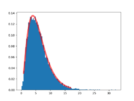
Figure 1: Illustration of the convergence of $\hat{T}_{n}$ to the $\chi^{2}_{6}$ distribution

3.5 Confidence regions and Tests

Let $\mathbb{K}=\left(K^{i}\right)_{1\leq i\leq r}\in\left(\mathcal{D}(\mathrm{I})\right)^{r}$. For $Q\in O(d)$ and $\mathcal{R}=\left(R_{i}\right)_{1\leq i\leq r}\in\mathcal{F}^{\mathrm{I}}$, set

$$\Delta_{\mathbb{K}}\left(Q,\mathcal{R}\right)=\frac{1}{4}\sum\limits_{i=1}^{r}\left\|K^{i}\mathrm{Log}_{P_{0}^{i}}^{G^{i}}\left(Q^{\prime}R_{i}Q\right)K^{i}\right\|_{F}^{2}\mathbf{1}_{\left\{Q^{\prime}R_{i}Q\notin\mathrm{Cut}\left(P_{0}^{i}\right)\right\}}.$$

Proposition 6.

For all $H\in O(\mathrm{I})$,

$$\Delta_{\mathbb{K}}\left(QH,\mathcal{R}\right)=\Delta_{\mathbb{K}}\left(Q,\mathcal{R}\right).$$ (3.5)

Proof.

First, we prove that for all $1\leq i\leq r$ and $H\in O(\mathrm{I})$,

$$(QH)^{\prime}R_{i}(QH)\notin\mathrm{Cut}\left(P_{0}^{i}\right)\iff Q^{\prime}R_{i}Q\notin\mathrm{Cut}\left(P_{0}^{i}\right)$$ (3.6)

Indeed, writing $R_{i}=C_{i}(C_{i})^{\prime}$ with $C_{i}\in\mathrm{St}(q_{i},d)$,

$$(QH)^{\prime}R_{i}(QH)\notin\mathrm{Cut}\left(P_{0}^{i}\right) \iff(H^{\prime}Q^{\prime}C_{i})(H^{\prime}Q^{\prime}C_{i})^{\prime}\notin\mathrm{Cut}\left(P_{0}^{i}\right)$$

$$\iff\mathrm{rank}\left(\left(I_{d}^{(i)}\right)^{\prime}\left(H^{\prime}Q^{\prime}C_{i}\right)\right)=q_{i}$$

$$\iff\mathrm{rank}\left(\left(HI_{d}^{(i)}\right)^{\prime}\left(Q^{\prime}C_{i}\right)\right)=q_{i}$$

Now, for all $1\leq i\leq r$, $\left(HI_{d}^{(i)}\right)\left(HI_{d}^{(i)}\right)^{\prime}=HP_{0}^{i}H^{\prime}=P_{0}^{i}$. Therefore,

$$\mathrm{rank}\left(\left(HI_{d}^{(i)}\right)^{\prime}\left(Q^{\prime}C_{i}\right)\right)=q_{i}\iff\mathrm{rank}\left(\left(I_{d}^{(i)}\right)^{\prime}\left(Q^{\prime}C_{i}\right)\right)=q_{i}\iff Q^{\prime}R_{i}Q\notin\mathrm{Cut}\left(P_{0}^{i}\right).$$

This proves $(\ref{equivCut})$. Now, when $(QH)^{\prime}R_{i}(QH)\notin\mathrm{Cut}\left(P_{0}^{i}\right)$, the closed formula for $\mathrm{Log}_{P_{0}^{i}}^{G^{i}}\left(\cdot\right)$ yields that

$$\mathrm{Log}_{P_{0}^{i}}^{G^{i}}\left((QH)^{\prime}R_{i}(QH)\right)=\mathrm{Log}_{P_{0}^{i}}^{G^{i}}\left(H^{\prime}(Q^{\prime}R_{i}Q)H\right)=H^{\prime}\mathrm{Log}_{P_{0}^{i}}^{G^{i}}\left(Q^{\prime}R_{i}Q\right)H.$$

Now, Remark 2 combined to the properties of invariance of the Frobenius norm imply that for all $1\leq i\leq r$,

$$\left\|K^{i}\left(H^{\prime}\mathrm{Log}_{P_{0}^{i}}^{G^{i}}\left(Q^{\prime}R_{i}Q\right)H\right)K^{i}\right\|_{F}=\left\|H^{\prime}\left(K^{i}\mathrm{Log}_{P_{0}^{i}}^{G^{i}}\left(Q^{\prime}R_{i}Q\right)K^{i}\right)H\right\|_{F}=\left\|K^{i}\mathrm{Log}_{P_{0}^{i}}^{G^{i}}\left(Q^{\prime}R_{i}Q\right)K^{i}\right\|_{F}$$

∎

For fixed $n\geq 1$, set $\widehat{\mathbb{K}}_{n}:=\left(\widehat{K}^{i}_{n}\right)_{1\leq i\leq r}\in\left(\mathcal{D}(\mathrm{I})\right)^{r}$ and define the map $\widehat{T}_{n}:O(d)\longrightarrow[0,\infty)$ by

$$\widehat{T}_{n}(Q):=n\Delta_{\widehat{\mathbb{K}}_{n}}\left(Q,F^{\mathrm{I}}\left(\widehat{\Sigma}_{n}\right)\right).$$

Then, for any matrix $\Gamma$ of eigenvectors of $\Sigma$, $\widehat{T}_{n}(\Gamma)$ is the pivotal statistic $\widehat{T}_{n}$ defined in $(\ref{PivotStat})$. Furthermore, Proposition 6 implies that the value of $\widehat{T}_{n}(Q)$ is independent of the class of $Q$ modulo $O(\mathrm{I})$.

Corollary 3.

For any $\alpha\in(0,1)$, a confidence region for $F^{\mathrm{I}}\left(\Sigma\right)$ of asymptotic level $(1-\alpha)$ is given by

$$R_{n,\alpha}:=\left\{\pi^{\mathrm{I}}(Q)\in\mathcal{F}^{\mathrm{I}}:\widehat{T}_{n}(Q)\leq\chi^{2}_{\mathrm{D}^{\mathrm{I}}}(1-\alpha)\right\},$$

where $\chi^{2}_{\mathrm{D}^{\mathrm{I}}}(1-\alpha)$ is the quantile of order $(1-\alpha)$ of the $\chi^{2}_{\mathrm{D}^{\mathrm{I}}}$ distribution.

Corollary 4.

Consider the following null hypothesis assumption.

$H_{0}$ : $\pi^{\mathrm{I}}\left(Q_{0}\right)=F^{\mathrm{I}}\left(\Sigma\right)$, for $Q_{0}\in O(d)$.

For any $\alpha\in(0,1)$, consider the test which accepts $H_{0}$ when $\widehat{T}_{n}(Q_{0})\leq\chi^{2}_{\mathrm{D}^{\mathrm{I}}}(1-\alpha)$ and reject $H_{0}$ else. Then, this test is of asymptotic level $\alpha$.

3.6 Conclusion

Given a normally distributed random vector $X$ valued in $\mathbb{R}^{d}$, $d\geq 1$, a geometric framework allows us to develop an asymptotic procedure to infer the set of all its PS’s. In addition, we provide easily implementable tests concerning the complete collection of principal subspaces and confidence regions for them. These results opens many questions which could lead to useful extensions. Among them, two of the most striking questions are:

• How to estimate or learn the type $\mathrm{I}$?

• Is it possible to relax the Gaussian assumption?

Acknowledgements

The authors have received funding from the European Research Council (ERC) under the European Union’s Horizon 2020 research and innovation program (grant agreement G-Statistics No 786854). It was also supported by the French government through the 3IA Côte d’Azur Investments ANR-19-P3IA-0002 managed by the National Research Agency.

References

• (1) Anderson, T.W. (1963). Asymptotic theory for principal components analysis. Ann. Math. Stat. (1963), Vol. 34, 122-148.
• (2) Batzies, E., Huper, K., Machado, L. and Silva Leite, F. (2015). Geometric mean and geodesic regresssion on Grassmannians. Linea Algebra Appl., 466:83-101, 2015.
• (3) Bhattacharya, R. and Patrangenaru, V. (2005). Large sample theory of intrinsic and extrinsic sample means on manifolds-II. The Annals of Statistics (2005), Vol. 33, No. 3, 1225-1259.
• (4) Bendokat, T., Zimmermann, R., Absil, P.A. (2020). A Grassmann Manifold Handbook: Basic Geometry and Computational Aspects. arXiv preprint arXiv:2011.13699, 2020.
• (5) Lee, J.M. (2018). Introduction to Riemannian manifolds. volume 176 of Graduate Texts in Mathematics. Springer, Cham, 2018.
• (6) Tyler, D.E. (1981). Asymptotic inference for eigenvectors. The Annals of Statistics 9 (4), 725-736, 1981.
• (7) Van der Vaart, A.W. (2000). Asymptotic Statistics. Cambridge Series in Statistical and Probabilistic Mathematics, Volume 3.
• (8) Ye, K., Wong, K.S.W., Lim, L.H. (2022). Optimization on flag manifolds. Mathematical Programming (Series A), 2022, 194(1-2), pp. 621-660.