Mass splitting and spin alignment for $\phi$ mesons in a magnetic field in NJL model

Abstract

Based on the Nambu-Jona-Lasinio (NJL) model, we develop a framework for calculating the spin alignment of vector mesons and applied it to study $\phi$ mesons in a magnetic field. We calculate mass spectra for $\phi$ mesons and observe mass splitting between the longitudinally polarized state and transversely polarized states. The $\phi$ meson in a thermal equilibrium system is preferred to occupy the state with spin $\lambda=0$ than those with spin $\lambda=\pm 1$, because the former state has a smaller energy. As a consequence, we conclude that the spin alignment will be larger than 1/3 if one measures along the direction of the magnetic field, which is qualitatively consistent with the recent STAR data. Around the critical temperature $T_{C}=150$ MeV, the positive deviation from 1/3 is proportional to the square of the magnetic field strength, which agrees with the result from the non-relativistic coalescence model. Including the anomalous magnetic moments for quarks will modify the dynamical masses of quarks and thus affect the mass spectra and spin alignment of $\phi$ mesons. The discussion of spin alignment in the NJL model may help us better understand the formation of hadron’s spin structure during the chiral phase transition.

I Introduction

Non-central relativistic heavy-ion collisions provide a unique opportunity to study quantum chromodynamics (QCD) matter in a strong magnetic field (Rafelski and Muller, 1976). The hot and dense matter created in collisions is known as the quark-gluon plasma (QGP), which evolves with time and cools down to the hadronic phase at the freeze-out time. In Au-Au collisions at the Relativistic Heavy Ion Collider (RHIC) or Pb-Pb collisions at the Large Hadron Collider (LHC), the magnetic field perpendicular to the reaction plane can reach $5\,m_{\pi}^{2}\sim 10^{18}$ Gauss ($m_{\pi}$ is the pion mass) or even larger (Kharzeev et al., 2008; Skokov et al., 2009; Kharzeev et al., 2013; Deng and Huang, 2012; Tuchin, 2013). Such a strong magnetic field is mainly generated by spectators in the colliding nuclei. It drops fastly with time, but the existence of medium electrical conductivity will extend its lifetime (McLerran and Skokov, 2014; Gursoy et al., 2014; Tuchin, 2015; Li et al., 2016; Chen et al., 2021; Yan and Huang, 2021; Wang et al., 2022). Therefore it may have sizeable contributions to many phenomena, for example, the chiral magnetic effect (Kharzeev et al., 2008; Fukushima et al., 2008; Son and Surowka, 2009), the $\Lambda$’s polarization (Liang and Wang, 2005a; Becattini et al., 2017; Adamczyk et al., 2017), and the charge-odd directed flow (Gursoy et al., 2014; Das et al., 2017; Gürsoy et al., 2018; Dubla et al., 2020; Zhang et al., 2022). On the other hand, the electromagnetic fields also have event-by-event fluctuations, which are still significantly large even in the late stage of collisions (Bzdak and Skokov, 2012; Deng and Huang, 2012; Siddique et al., 2021). The fluctuating fields thus contribute to phenomena at the freeze-out time, such as the magnetic catalysis (Klimenko, 1992; Gusynin et al., 1994, 1996; Miransky and Shovkovy, 2002; Endrodi et al., 2019), the inverse magnetic catalysis (Bali et al., 2012; Endrodi et al., 2019), and the phase structure of the QGP (Gusynin et al., 1994; Fraga and Mizher, 2009; Mizher et al., 2010; Andersen et al., 2016).

Recently, the STAR collaboration has measured the $\phi$ and $K^{*0}$ meson’s spin alignment along the out-of-plane direction and observes a significant positive deviation from 1/3 for the $\phi$ meson (Abdallah et al., 2022). The spin alignment refers to the 00-element of the normalized spin density matrix for a vector meson with spin-1 (Liang and Wang, 2005b; Tang et al., 2018). The positive derivation from 1/3 observed in experiments indicates that the spin of $\phi$ meson is preferred to align in the reaction plane. According to the quark coalescence model, the spin alignment of vector meson is induced by polarizations of its constituent quarks (Liang and Wang, 2005b; Yang et al., 2018) and thus have various sources such as the vorticity field (Liang and Wang, 2005b; Yang et al., 2018; Xia et al., 2021), the electromagnetic field (Yang et al., 2018), the helicity polarization (Gao, 2021), the turbulent color field (Müller and Yang, 2022), the shear stress (Li and Liu, 2022; Wagner et al., 2022), and the strong force field (Sheng et al., 2020a, b, 2022a, 2022b). Among these works, only the fluctuations of the strong force field successfully reproduce the experiment data (Sheng et al., 2022b). Since the strong force field in (Sheng et al., 2022b) has the same structure as the classical electromagnetic field, one naturally expects that fluctuations of electromagnetic fields, rather than their event-average values, also contribute to the spin alignment of vector mesons.

In this work, we study the spin alignment of $\phi$ meson in a constant magnetic field using the three flavor Nambu-Jona-Lasinio (NJL) model (Nambu and Jona-Lasinio, 1961a, b; Klimt et al., 1990; Vogl et al., 1990; Klevansky, 1992; Buballa, 2005; Volkov and Radzhabov, 2006; Fukushima, 2008). Such a field configuration can be straightforwardly extended to the case of a space-time dependent magnetic field with the typical length of its inhomogeneity much larger than the typical hadron size. In the NJL model, gluons are integrated out and quarks interact via local four-fermion interactions, which have the form that keeps the chiral symmetry. Mesons are treated as quantum fluctuations beyond a constant mean-field and their propagators are introduced through the random phase approximation by the resummation of quark bubbles (Klevansky, 1992; Hatsuda and Kunihiro, 1994; Buballa, 2005). The mass spectra for mesons are given by the poles, of their propagators. Within the framework of magnetized NJL model, the spectra of light-flavor mesons, including $\sigma$, $\pi^{0}$, $\pi^{\pm}$, $\omega$, $\rho^{0}$, and $\rho^{\pm}$, have attracted a lot of interest (Liu et al., 2015; Avancini et al., 2016, 2017; Mao, 2019; Coppola et al., 2018; Chaudhuri et al., 2019; Xu et al., 2021; Wei et al., 2020; Yang et al., 2022), but few works focus on the $\phi$ meson. One can refer to (Andersen et al., 2016; Miransky and Shovkovy, 2015; Cao, 2021) for recent reviews on the NJL model in a strong magnetic field. In this manuscript, we observe the splitting between masses of $\phi$ mesons in different spin states, which is induced by the magnetization of the constituent quark and antiquark. In a hot and thermal equilibrium system, the mass splitting leads to different spin-dependent equilibrium distributions and thus corresponds to a nontrivial spin alignment. We also study the effect of quark anomalous magnetic moments (AMM) considering that constituent quarks have different magnetic moments compared with free quarks (Brekke and Rosner, 1988; Chang et al., 2011; Fayazbakhsh and Sadooghi, 2014; Ayala et al., 2016; Chaudhuri et al., 2019; Xu et al., 2021). The AMMs are included in the fermion Hamiltonian by putting a new term $q_{f}\kappa_{f}F_{\mu\nu}\sigma^{\mu\nu}/2$, where $F^{\mu\nu}$ is the electromagnetic field tensor, $\sigma^{\mu\nu}\equiv(i/2)[\gamma^{\mu},\gamma^{\nu}]$, and $q_{f}$, $\kappa_{f}$ are the charge and the AMM for a quark with flavor $f=u,d,s$. The AMMs change the dynamical masses of quarks and therefore affect the spectra and spin alignment of the $\phi$ meson.

This manuscript is organized as follows. In Sec. II we review the theoretical framework for the three flavor NJL model and numerically calculate quark dynamical masses. Then in Sec. III we give analytical formulas for the vector meson’s propagator, the spectral function, and the spin alignment. Numerical results for $\phi$ mesons are given in Sec. IV. We then repeated the calculations in the presence of nonzero AMMs in Sec. V. Finally, in Sec. VI we summarize our findings and conclude.

II Nambu-Jona-Lasinio model for quarks

II.1 Theoretical framework

In order to describe a strongly-interaction quark matter, we use the three-flavor Nambu-Jona-Lasinio model with scalar and vector channels of four-fermion interactions (Klevansky, 1992; Hatsuda and Kunihiro, 1994; Buballa, 2005; Volkov and Radzhabov, 2006),

$$\mathcal{L}_{\text{eff}} =\mathcal{L}_{q}+G_{S}\sum_{a=0}^{8}\left[(\overline{\psi}\lambda_{a}\psi)^{2}+(\overline{\psi}i\gamma_{5}\lambda_{a}\psi)^{2}\right]$$

$$-G_{V}\sum_{a=0}^{8}\left[(\overline{\psi}\gamma_{\mu}\lambda_{a}\psi)^{2}+(\overline{\psi}i\gamma_{\mu}\gamma_{5}\lambda_{a}\psi)^{2}\right]$$

$$-K\left\{\text{det}_{f}\left[\overline{\psi}(1+\gamma_{5})\psi\right]+\text{det}_{f}\left[\overline{\psi}\left(1-\gamma_{5}\right)\psi\right]\right\}\,,$$ (1)

where $\psi=(\psi_{u},\psi_{d},\psi_{s})$ are Dirac spinors for $u$, $d$, and $s$ quarks, respectively, $\lambda_{a}$ with $a=1,2,\cdots,8$ are Gell-Mann matrices, and $\lambda_{0}=\sqrt{2/3}I_{0}$ with $I_{0}$ being the identity matrix in the color space. The last term in Eq. (1) is the six-quark Kobayashi-Maskawa - ’t Hooft interaction that breaks the $U_{A}(1)$ symmetry (’t Hooft, 1976). Here $G_{S}$ and $G_{V}$ are coupling constants for scalar and vector interactions, respectively. The Lagrangian $\mathcal{L}_{q}$ for quarks in an external electromagnetic field is given by

$$\mathcal{L}_{q}=\sum_{f=u,d,s}\overline{\psi}_{f}\left(i\gamma_{\mu}D_{f}^{\mu}-m_{f}\right)\psi_{f}\,,$$ (2)

where $m_{f}$ denotes current mass for quarks with flavor $f=u,d,s$. The covariant derivative is $D_{f}^{\mu}\equiv\partial^{\mu}+iq_{f}A^{\mu}$ with $q_{f}$ being the quark charges and $A^{\mu}$ being the gauge potential for the external electromagnetic field. Under the mean-field approximation, the Lagrangian becomes

$$\mathcal{L}_{\text{MF}} = \sum_{f=u,d,s}\overline{\psi}_{f}\left(i\gamma_{\mu}D_{f}^{\mu}-M_{f}\right)\psi_{f}$$ (3)

$$-2G_{S}\sum_{f=u,d,s}\sigma_{f}^{2}+4K\sigma_{u}\sigma_{d}\sigma_{s}\,,$$

where $\sigma_{f}$ is the quark chiral condensate $\sigma_{f}\equiv\left\langle\overline{\psi}_{f}\psi_{f}\right\rangle$. Here we only consider the chiral condensate and set all other possible condensates to zeros. The dynamical mass $M_{f}$ is related to $\sigma_{f}$ as

$$M_{f}\equiv m_{f}-4G_{S}\sigma_{f}+2K\prod_{f^{\prime}\neq f}\sigma_{f^{\prime}}\,,$$ (4)

where the last term arises from the ’t Hooft interaction.

We consider quarks in a constant magnetic field. Without loss of generality, we assume the magnetic field is along the positive $z$-direction and take the Landau gauge $A^{\mu}=(0,0,Bx,0)$. For each flavor of quark, it is straightforward to derive the Dirac equation from the Lagrangian (3). The Dirac equation can be analytically solved by applying the Ritus method (Ritus, 1972, 1978), resulting in the following dispersion relation for the $n$-th Landau level,

$$E=\pm E_{f,n}(p_{z})=\pm\sqrt{p_{z}^{2}+M_{f}^{2}+2n|q_{f}B|}\,,$$ (5)

where the momentum perpendicular to the $z$-direction is quantized as the Landau levels, while the longitudinal momentum is not restricted. Here $B>0$ denotes the magnetic field strength and $q_{f}$ is the electric charge of a quark with flavor $f$, with $q_{u}=(2/3)e$, $q_{d}=q_{s}=(-1/3)e$, and $e$ being the elementary charge. The positive and negative energies are related to particles and antiparticles, respectively. Using Eq. (5), the quark grand thermodynamic potential $\Omega_{f}$ can be written as

$$\Omega_{f} =\frac{N_{c}|q_{f}B|}{4\pi^{2}}\sum_{n,s}\int dp_{z}\Biggl{\{}\frac{E_{f,n}(p_{z})}{2}$$

$$+2T\ln\left[1+e^{-E_{f,n}(p_{z})/T}\right]\Biggr{\}}\,,$$ (6)

where $T$ is the temperature and $N_{c}=3$ is the degeneracy of color. The summation in Eq. (6) runs over $s=+$ for the lowest Landau level $n=0$ and $s=\pm$ for other Landau levels $n=1,2,3,\cdots$. The total grand potential for the whole system includes $\Omega_{f}$ and the mean field part, which is given by

$$\Omega=\sum_{f=u,d,s}\left(2G_{S}\sigma_{f}^{2}-\Omega_{f}\right)+4K\sigma_{u}\sigma_{d}\sigma_{s}\,.$$ (7)

The quark condensates $\sigma_{f}$ and the corresponding quark masses $M_{f}$ are then calculated by minimizing the grand potential, $\partial\Omega/\partial\sigma_{f}=0$.

II.2 Numerical results

Since the NJL model is non-renormalizable, it is necessary to include a regularization scheme for the divergent momentum integrals in Eqs. (6). Since a sharp three-momentum cutoff will lead to nonphysical oscillations in the presence of a magnetic field, we choose a Pauli-Villas regularization scheme (Pauli and Villars, 1949). Any function of $M_{f}$ is replaced by a summation,

$$f(M_{f})\rightarrow f_{\text{P.V.}}(M_{f})=\sum_{j=0}^{3}c_{j}f\left(\sqrt{M_{f}^{2}+j\Lambda^{2}}\right)\,,$$ (8)

with $c_{0}=1$, $c_{1}=-3$, $c_{2}=3$, and $c_{3}=-1$. We take the parameter set given in (Carignano and Buballa, 2020),

$$m_{u,d}=10.3\,\text{MeV}, m_{s}=236.9\,\text{MeV}, \Lambda=0.7812\,\text{GeV},$$

$$G_{S}\Lambda^{2}=4.90, K\Lambda^{5}=129.8,$$ (9)

which are obtained by fitting vacuum values for the pion decay constant and masses of pion, kaon, $\eta^{\prime}$, while fixing the vacuum mass for light-quarks to $M_{u,d}=325$ MeV. For the strange quark, this set of parameters leads to a dynamical mass $M_{s}=554$ MeV in the vacuum in absence of the magnetic field.

We first focus on dynamical masses for quarks, which are related to the chiral condensates $\sigma_{f}$ as given in Eq. (4). The condensates $\sigma_{f}$ are order parameters for the chiral phase transition. In the chiral symmetry breaking phase, $\sigma_{f}\neq 0$ and thus quarks have nonvanishing dynamical masses. In the chiral symmetry restored phase, $\sigma_{f}=0$ and quark dynamical masses reduce to their current masses. The behavior of dynamical masses for $u$, $d$, and $s$ quarks as functions of the temperature is shown in Fig. 1. Here we choose two sets of values for the magnetic field strength: solid lines for $eB=0$ and dashed lines for $eB=10\,m_{\pi}^{2}$. We observe that the chiral phase transition is a cross-over with critical temperature around $T_{C}\approx 150$ MeV. Compared to the case with $eB=0$, a nonzero magnetic field, $eB=10\,m_{\pi}^{2}$, corresponds to larger quark masses and slightly higher $T_{C}$, which is the behavior of the magnetic catalysis. We also observe that the $u$ and $d$ quarks have identical masses when $eB=0$, but have different masses in a nonzero magnetic field. That is because the difference in their electric charges, $q_{u}=(2/3)e$ and $q_{d}=(-1/3)e$, leads to different magnetic energies and breaks the symmetry between light-flavor quarks.

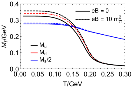
Figure 1: Dynamical masses as functions of the temperature for $u$ quark (black lines), $d$ quark (red lines), and $s$ quark (blue lines). The magnetic field strength is set to $eB=0$ (solid lines) or $eB=10\,m_{\pi}^{2}$ (dashed lines).

In order to explicitly show the magentic field dependence, we plot in Fig. 2 the ratio of quark masses as functions of the field strength to those in absence of the magnetic field. Here we fix the temperature at the ordinary critical temperature $T=150$ MeV. We find that quark masses grow with an increasing magnetic field, which is the phenomena of magnetic catalysis. The $u$ quark mass is more affected by the magnetic field than the $d$ quark mass since $|q_{u}|>|q_{d}|$. On the other hand, the $s$ quark is less affected by the magnetic field because $s$ quark has a larger dynamical mass than $u,\,d$ quarks.

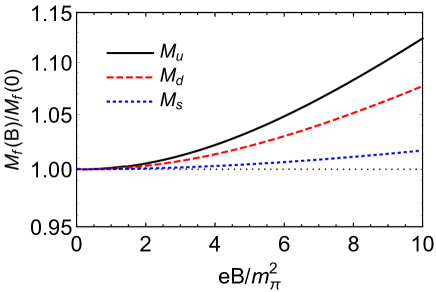
Figure 2: Dynamical masses as functions of the magnetic field strength at $T=150$ MeV for $u$, $d$, and $s$ quarks, denoted by the black solid line, the red dashed line, and the blue dotted line, respectively. The masses are normalized by the corresponding values in absence of magnetic field.

III Spin alignment for $\phi$ mesons in NJL model

III.1 Propagator for $\phi$ mesons

In the NJL model, mesons are described as excitations beyond the mean field. The progator of a meson is obtained by taking the quark bubble summation in the random phase approximation, corresponding to the Dyson-Schwinger equation shown in Fig. 3. For the vector meson channel, the Dyson-Schwinger equation is given by

$$D^{\mu\nu}(k)=4G_{V}\Delta^{\mu\nu}(k)+4G_{V}\Delta^{\mu\alpha}(k)\Sigma_{\alpha\beta}(k)D^{\beta\nu}(k)\,,$$ (10)

where $D^{\mu\nu}$ is the vector meson’s propagator and $\Sigma^{\mu\nu}$ is the self-energy tensor. The projection operator $\Delta^{\mu\nu}(k)\equiv g^{\mu\nu}-k^{\mu}k^{\nu}/k^{2}$ ensures the Ward identity $k_{\mu}D^{\mu\nu}(k)=0$. Using the quark propator $S_{f}(p)$, the self-energy at one-quark-loop level is given by

$$\Sigma^{\mu\nu}(k)=-iN_{c}\int\frac{d^{4}p}{(2\pi)^{4}}\text{Tr}\left[\gamma^{\mu}S_{f}(k+p)\gamma^{\nu}S_{f^{\prime}}(p)\right]\,,$$ (11)

where the quark flavors $f$ and $f^{\prime}$ depend on the type of considered meson. In this work we focus the $\phi$ meson and thus we take $f=f^{\prime}=s$ in Eq. (11). Following Ref. (Miransky and Shovkovy, 2015), the quark propagator in momentum space is expressed as follows,

$$S_{f}(p)=ie^{-p_{\perp}^{2}/|q_{f}B|}\sum_{n=0}^{\infty}\frac{(-1)^{n}D_{n}^{f}(p)}{(k^{0})^{2}-[E_{f,n}(k_{z})]^{2}+i\epsilon}$$ (12)

where the poles are shifted above or below the real axis by an infinite small imaginary part $\pm i\epsilon$ such that $S_{f}(p)$ denotes the Feynmann propagator. The residue at each pole energy is determined by the function in the numerator,

$$D_{n}^{f}(p) = 2(p^{0}\gamma^{0}-p_{z}\gamma^{3}+M_{f})\left[\mathcal{P}_{+}L_{n}\left(\frac{2p_{\perp}^{2}}{|q_{f}B|}\right)\right.$$ (13)

$$\left.-\mathcal{P}_{-}L_{n-1}\left(\frac{2p_{\perp}^{2}}{|q_{f}B|}\right)\right]$$

$$+4{\bf p}_{\perp}\cdot\boldsymbol{\gamma}_{\perp}L_{n-1}^{1}\left(\frac{2p_{\perp}^{2}}{|q_{f}B|}\right)$$

where the projection operators are $\mathcal{P}_{\pm}=[1\pm i\gamma^{1}\gamma^{2}\text{sgn}(q_{f}B)]/2$ and $L_{n}^{i}(x)$ are associated Laguerre polynomials with $L_{n}(x)\equiv L_{n}^{0}(x)$.

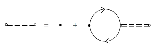
Figure 3: Dyson-Schwinger equation for meson’s propagator. Solid lines denote quark propagators, dashed lines denote meson propagator, black dots denotes four-quark vertexes, and white dots denotes the quark-meson vertexes.

As spin-1 particles, the vector mesons have three spin states, $\lambda=0,\,\pm 1$. Taking the spin quantization direction as the $z$-direction in the meson’s rest frame, which is the same as the direction of magnetic field, we have the following spin polarization vectors,

$$\boldsymbol{\epsilon}_{0} = (0,0,1)\,,$$

$$\boldsymbol{\epsilon}_{+1} = -\frac{1}{\sqrt{2}}(1,i,0)\,,$$

$$\boldsymbol{\epsilon}_{-1} = \frac{1}{\sqrt{2}}(1,-i,0)\,,$$ (14)

corresponding to $\lambda=0,\pm 1$, respectively. By taking a Lorentz boost, we derive the covariant form of spin polarization vectors,

$$\epsilon^{\mu}(\lambda,k)=\left(\frac{{\bf k}\cdot\boldsymbol{\epsilon}_{\lambda}}{m_{V}},\boldsymbol{\epsilon}_{\lambda}+\frac{{\bf k}\cdot\boldsymbol{\epsilon}_{\lambda}}{m_{V}(\omega+m_{V})}{\bf k}\right)\,,$$ (15)

where $k^{\mu}\equiv(\omega,{\bf k})$ is the four-momentum and $m_{V}=\sqrt{\omega^{2}-{\bf k}^{2}}$ is the mass of the vector meson. It is easy to check that these vectors are perpendicular to $k^{\mu}$, $k_{\mu}\epsilon^{\mu}(\lambda,k)=0$, and they are properly normalized as $\epsilon^{\mu\ast}(\lambda,k)\epsilon_{\mu}(\lambda^{\prime},k)=-\delta_{\lambda\lambda^{\prime}}$. They also form a complete basis as $\sum_{\lambda=0,\pm 1}\epsilon^{\mu\ast}(\lambda,k)\epsilon^{\nu}(\lambda,k)=-\Delta^{\mu\nu}(k)$. Then the meson propagator $D^{\mu\nu}(k)$ can be cast into the following form,

$$D^{\mu\nu}(k)=\sum_{\lambda,\lambda^{\prime}=0,\pm 1}\epsilon^{\ast\mu}(\lambda,k)\epsilon^{\nu}(\lambda^{\prime},k)D_{\lambda\lambda^{\prime}}(k)\,,$$ (16)

where the element $D_{\lambda\lambda^{\prime}}(k)$ is a Lorentz invariant function that is derived by projecting $D^{\mu\nu}(k)$ onto $\epsilon_{\mu}(\lambda,k)\epsilon_{\nu}^{\ast}(\lambda^{\prime},k)$,

$$D_{\lambda\lambda^{\prime}}(k)=\epsilon_{\mu}(\lambda,k)\epsilon_{\nu}^{\ast}(\lambda^{\prime},k)D^{\mu\nu}(k)\,.$$ (17)

Similarly, projecting the Dyson-Schwinger equation in (10) onto $\epsilon_{\mu}(\lambda,k)\epsilon_{\nu}^{\ast}(\lambda^{\prime},k)$ gives the equation for $D_{\lambda\lambda^{\prime}}(k)$,

$$D_{\lambda\lambda^{\prime}}(k)=-4G_{V}\delta_{\lambda\lambda^{\prime}}-4G_{V}\sum_{\lambda_{1}=0,\pm 1}\Sigma_{\lambda\lambda_{1}}(k)D_{\lambda_{1}\lambda^{\prime}}(k)\,,$$ (18)

where the self-energy matrix element in the spin space, $\Sigma_{\lambda\lambda^{\prime}}(k)$, is defined as

$$\Sigma_{\lambda\lambda^{\prime}}(k)=\epsilon_{\mu}(\lambda,k)\epsilon_{\nu}^{\ast}(\lambda^{\prime},k)\Sigma^{\mu\nu}(k)\,.$$ (19)

Equation (18) has the following formal solution,

$$D_{\lambda\lambda^{\prime}}(k)=-\left[\frac{4G_{V}}{1+4G_{V}\Sigma(k)}\right]_{\lambda\lambda^{\prime}}\,.$$ (20)

where $1$ and $\Sigma(k)$ in the denominator are short-handed notations for the $3\times 3$ unit matrix and the matrix $\Sigma_{\lambda\lambda^{\prime}}(k)$.

III.2 Spectral function and spin alignment

In a thermal equilibrium system, the meson’s propagator can be expressed in the spectral representation as (Kapusta and Gale, 2011)

$$D^{\mu\nu}(k)=n_{\text{BE}}(\omega/T)\frac{1}{\pi}\text{Im}D^{\mu\nu}(k)\,,$$ (21)

where $n_{\text{BE}}(\omega/T)=1/(e^{\omega/T}-1)$ is the Bose-Einstein distribution. The density matrix for the vector meson is the given by

$$\overline{\rho}_{\lambda\lambda^{\prime}}({\bf k})=\int d\omega\,2\omega\,n_{\text{BE}}(\omega/T)\xi_{\lambda\lambda^{\prime}}(k)\,,$$ (22)

where the spectral function is derived from the imaginary part of the full propagator,

$$\xi_{\lambda\lambda^{\prime}}(k)\equiv\frac{1}{\pi}\epsilon_{\mu}(\lambda,k)\epsilon_{\nu}^{\ast}(\lambda^{\prime},k)\text{Im}D^{\mu\nu}(k)\,.$$ (23)

In Eq. (22), we integrate over $\omega$ so that the diagonal element $\overline{\rho}_{\lambda\lambda}({\bf k})$ has definite physical meaning of particle number for vector mesons with spin $\lambda$ and three-momentum ${\bf k}$. The spin alignment is then given by the $00$-element of the normalized density matrix,

$$\rho_{00}({\bf k})\equiv\frac{\overline{\rho}_{00}({\bf k})}{\sum_{\lambda=0,\pm 1}\overline{\rho}_{\lambda\lambda}({\bf k})}\,.$$ (24)

The result in a constant magnetic field can be evaluated by using Eqs. (11), (12), and (21) - (24). When calculating the self-energy in (11), we substitute the energy integral with a summation over Matsubara frequencies at finite temperature (Kapusta and Gale, 2011). This allows us to study the meson properties at finite temperature.

We emphasize that Eqs. (21) - (24) are universal formulas, which can be applied in calculating momentum-dependent spin alignments along any measuring direction. However, it will significantly simplify our calculation to focus on a static meson ${\bf k}={\bf 0}$ and choose the measuring direction as the $z$-direction. The corresponding spin polarization vectors as given in Eqs. (14) and (15). Due to the rotational invariance in the $x-y$ plane, one can also prove that $\Sigma_{\lambda\lambda^{\prime}}$, $D_{\lambda\lambda^{\prime}}$, and the density matrix $\overline{\rho}_{\lambda\lambda^{\prime}}({\bf 0})$ are diagonal in the spin space,

$$\overline{\rho}_{\lambda\lambda^{\prime}}({\bf 0})=\left(\begin{array}[]{ccc}\overline{\rho}_{11}&0&0\\ 0&\overline{\rho}_{00}&0\\ 0&0&\overline{\rho}_{-1,-1}\end{array}\right)\,,$$ (25)

where the states with $\lambda=\pm 1$ are degenerate, $\overline{\rho}_{-1,-1}=\overline{\rho}_{11}$. In general, if the measuring direction is characterized by Euler angles $(\alpha,\,\beta,\,\gamma)$, the density matrix is calculated by performing a rotation in spin space,

$$\overline{\rho}_{\lambda\lambda^{\prime}}({\bf 0};\alpha,\beta,\gamma)$$

$$\ \ =\sum_{\lambda_{1},\lambda_{2}}R_{\lambda\lambda_{1}}(\alpha,\beta,\gamma)\overline{\rho}_{\lambda_{1}\lambda_{2}}({\bf 0})R_{\lambda_{2}\lambda^{\prime}}^{-1}(\alpha,\beta,\gamma)\,,$$ (26)

where $R_{\lambda\lambda^{\prime}}(\alpha,\beta,\gamma)$ is the spin-1 representation of the rotation with Euler angles $(\alpha,\,\beta,\,\gamma)$. Here $\overline{\rho}_{\lambda_{1}\lambda_{2}}({\bf 0})$ is the density matrix when measuring along the $z$-direction. A straightforward calculation shows that the spin alignment is independent to Euler angles $\alpha$ and $\gamma$,

$$\rho_{00}({\bf 0};\alpha,\beta,\gamma)=\frac{\overline{\rho}_{00}({\bf 0})\cos^{2}\beta+\overline{\rho}_{11}({\bf 0})\sin^{2}\beta}{\overline{\rho}_{00}({\bf 0})+2\overline{\rho}_{11}({\bf 0})}\,.$$ (27)

Defining the spin alignment in the magnetic field direction as

$$\rho_{00}^{B}({\bf 0})\equiv\frac{\rho_{00}({\bf 0})}{\rho_{00}({\bf 0})+2\rho_{11}({\bf 0})}\,,$$ (28)

we derive that

$$\rho_{00}({\bf 0};\alpha,\beta,\gamma)=\frac{1}{2}\left\{1-\rho_{00}^{B}({\bf k})+\left[3\rho_{00}^{B}({\bf k})-1\right]\cos^{2}\beta\right\}\,,$$ (29)

which only depends on $\rho_{00}^{B}$ and the angle between the direction of the magnetic field and the measuring direction. For a fluctuating magnetic field, one has to take an average over the $\beta$-angle and the field strength. If the field does not have a preferred direction, one can prove that the average $\left\langle\rho_{00}({\bf 0};\alpha,\beta,\gamma)\right\rangle=1/3$, as expected. If the fluctuations are anisotropic in space, the average spin alignment will deviate from 1/3, as predicted in Refs. (Sheng et al., 2020a, b, 2022a, 2022b).

IV Numerical results for $\phi$ mesons

The property of vector meson depends on the coupling strength $G_{V}$ for the vector channel in the Lagrangian (1). In our calculation, we take

$$G_{V}\Lambda^{2}=-4.67\,,$$ (30)

which is determined by fitting the $\phi$ meson’s vacuum mass $M_{\phi}=1.02$ GeV in the absence of magnetic field.

IV.1 Mass spectra for $\phi$ meson

Using quark masses as functions of the temperature and the magnetic field strength discussed in Sec. II.2, we are then able to calculate the vector meson’s spectral functions from Eqs. (11), (12), and (23). In this work, we focus on the vector $\phi$ meson, which has constituent quarks $s$ and $\bar{s}$. At the one-loop level, the self-energy for the $\phi$ meson depends on the propagator of $s$ quark, but does not depend on propagators of $u$ and $d$ quarks. We set the spin quantization direction parallel to the magnetic field and therefore the spectral function is diagonal $\xi_{\lambda\lambda^{\prime}}=\text{diag($\xi_{+1},\,\xi_{0}$,\,$\xi_{-1}$)}$, and spin states $\lambda=\pm 1$ are degenerate, $\xi_{+1}=\xi_{-1}$. In this work, we only focus on static $\phi$ mesons, i.e., the three-momenta of meson are set to zeros, ${\bf k={\bf 0}}$.

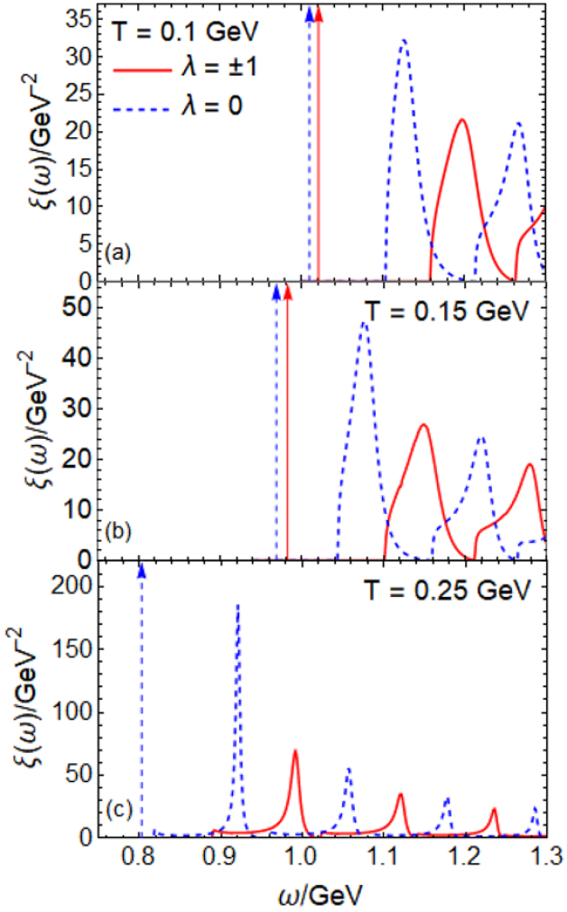
Figure 4: Spectral functions for $\phi$ mesons in a constant magnetic field with $eB=5m_{\pi}^{2}$, at $T=100$ MeV [panel (a)], $T=150$ MeV [panel (b)], and $T=250$ MeV [panel (c)]. Here red solid lines denote spectral functions for $\phi$ mesons with spin state $\lambda=\pm 1$ and blue dashed lines denote the spectral function of $\lambda=0$. Red and blue arrows correspond to delta functions.

In order to clearly show the influence of the magnetic field to the spectral function, we choose the magnetic field strength $eB=5\,m_{\pi}^{2}$ and plot the mass spectra for the $\phi$ meson at temperatures $T=100$ MeV, $150$ MeV, and $250$ MeV in Fig. 4. In general, the spectral function can be separated into a delta-function part and a continuum part as

$$\xi_{\lambda}(\omega,{\bf 0})=\delta(\omega^{2}-M_{\phi,\lambda}^{2})+\xi_{\lambda}^{\ast}(\omega)\,.$$ (31)

The delta-function part is identified as a stable bound state that corresponds to a real on-shell $\phi$ meson with mass $M_{\phi,\lambda}$. The continuum part $\xi_{\lambda}^{\ast}(\omega)$ is related to unstable resonance excitations. In Fig. 4, the delta-functions are plotted as arrows. We observe a mass splitting between bound states with $\lambda=0$ and $\lambda=\pm 1$ in Fig. 4 (a) and (b), indicating that the longitudinally polarized $\phi$ meson and the transversely polarized $\phi$ meson have different energies. The bound state masses and the thresholds for the continuum drop with increasing $T$, which is the result of the decreasing $s$ quark mass. The bound states will dissociate when $T$ is large enough, which is the Mott transition (MOTT, 1968; Hufner et al., 1996; Costa et al., 2003; Blaschke et al., 2017; Mao, 2021). In this work, the $\phi$ meson self-energy is purelly contributed by the $s$ quark loop since we only consider the coupling between the $\phi$ meson and the $s$ quark. In a thermal medium, the physical $\phi$ meson was observed to have a large broadening (Ishikawa et al., 2005; Muto et al., 2007; Qian et al., 2009), which may arise from $\phi N$ interations and is beyond the scope of our discussion. We also observe in Fig. 4 that the continuum parts contains several well-separated peaks. One can understand the multi-peak structure of the spectral function in Fig. 4 as follows. In the presence of a magnetic field, the dispersion relation of $s$ quark is quantized as Landau levels given in Eq. (5). Supposing the constituent $s$ and $\bar{s}$ quarks inside a $\phi$ meson are at Landau levels $n_{1}$ and $n_{2}$, respectively, the angular momentum conservation demands that the $\phi$ meson with $\lambda=0$ must be consist of quark and antiquark with $n_{1}=n_{2}$, and the $\phi$ meson with $\lambda=\pm 1$ correspond to $n_{1}=n_{2}\pm 1$. Different sets of $n_{1}$ and $n_{2}$ give different resonance peaks as shown in Fig. 4.

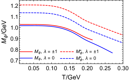
Figure 5: Dynamical masses as functions of the temperature for $\phi$ mesons at $eB=5\,m_{\pi}^{2}$. Masses for bound states with spin $\lambda=0$ and $\lambda=\pm 1$ are plotted with red solid lines and blue solid lines, respectively, while those for resonance excitations are plotted with red dashed lines and blue dashed lines, respectively.

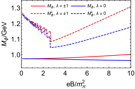
Figure 6: Dynamical masses as functions of $eB$ for $\phi$ mesons at $T=150$ MeV. Notations are the same as in Fig. 5.

Denoting the energy for the most significant peak in the continuum as $M_{\phi,\lambda}^{\ast}$, we plot $M_{\phi,\lambda}^{\ast}$, and $M_{\phi,\lambda}$ for bound states, as functions of the temperature at $eB=5m_{\pi}^{2}$ in Fig. 5. Similar to the temperature dependence of the $s$ quark, the $\phi$ meson masses also decrease at higher temperatures. One can observe from Fig. 5 the mass splitting between states with $\lambda=0$ and $\lambda=\pm 1$, induced by the broken symmetry because of the magnetic field. States with $\lambda=0$ always have smaller masses compared to states with $\lambda=\pm 1$. As the temperature increases, the bound states finally dissociate, and the corresponding dissociation temperature is $215$ MeV for $\lambda=\pm 1$ and $270$ MeV for $\lambda=0$. Therefore when the temperature $215\,\text{MeV}<T<270\,\text{MeV}$, $\phi$ meson bound states are purely at states with $\lambda=0$. In Fig. 6, we show the field strength dependence for the $\phi$ meson masses.The mass for $\lambda=0$ bound-states decreases with an increasing $eB$, while that for $\lambda=\pm 1$ increases. Masses for resonance excitations oscillate when $eB<2.5\,m_{\pi}^{2}$, and is nearly linear in $eB$ when $2.5\,m_{\pi}^{2}<eB<10\,m_{\pi}^{2}$.

IV.2 Spin alignment for $\phi$ mesons

Substituting the spectral functions calculated in subsection IV.1 into Eqs. (22) and (24), we derive the $\phi$ meson’s spin alignment. Note that the bound states and resonance excitations are at different mass regions: the bound states have masses $\sim 1$ GeV or smaller, while masses for the resonance excitations have larger masses. Therefore we treat them as different kinds of particles and calculate their spin alignments separately.

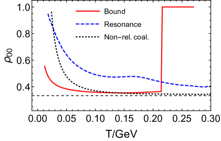
Figure 7: Spin alignments as functions of the temperature. The magnetic field strength is taken as $eB=5\,m_{\pi}^{2}$. Red solid lines are spin alignment for bound states, calculated using the delta-function part in the spectral function Eq. (31), while blue dashed lines are spin alignment for resonance excitations, calculated using the continuum part in Eq. (31). Black dash-dotted lines are results from the non-relativistic coalescence model, given in Eq. (32).

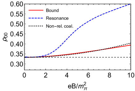
Figure 8: Spin alignments as functions of the magnetic field strength at temperature $T=150$ MeV. Notations are the same as in Fig. 7.

In Fig. 7, we plot spin alignments $\rho_{00}$ as functions of the temperature at $eB=5\,m_{\pi}^{2}$. Spin alignments for bound states and resonance excitations are denoted as red solid lines and blue dashed lines, respectively. As a comparison, we also plot the result from a non-relativistic coalescence model (Yang et al., 2018),

$$\rho_{00}^{\text{Non-rel. coal.}}=\frac{1}{3}+\frac{4}{9T^{2}}\mu_{s}^{2}B^{2}\,,$$ (32)

where $\mu_{s}=q_{s}/(2M_{s})$ is the magnetic moment for the $s$ quark, with $q_{s}=(-1/3)e$. The spin alignment $\rho_{00}$ for bound states, shown by the red solid line in Fig. 7, is significantly smaller than the result from the non-relativistic coalescence model (black dotted line) when $T<100$ MeV. The $\rho_{00}$ for bound states decreases towards $1/3$ with an increasing $T$. For the temperature $T=150$ MeV, $\rho_{00}$ for bound states is in very good agreement with the coalescence model. Above 150 MeV, $\rho_{00}$ for bound states is larger than the result from the coalescence model. Especially, bound states with $\lambda=\pm 1$ vanish when $T>215$ MeV, leading to the result of $\rho_{00}=1$ in this temperature region. On the other hand, the spin alignment $\rho_{00}$ for resonance states is always larger than the result from the coalescence model except at very low temperatures. In Fig. 8 we show spin alignments as functions of the magnetic field strength. We focus on a fixed temperature $T=150$ MeV and observe that $\rho_{00}$ increases with increasing $eB$. In the zero-field limit $eB\rightarrow 0$, $\rho_{00}$ agrees with $1/3$, as expected. We find that the spin alignment for bound states agrees with the result of the non-relativistic coalescence model, while the spin alignment for resonance excitations is significantly larger.

V Effect of anomalous magnetic field

Considering that constituent quark may have different magnetic moments compared with free quarks (Brekke and Rosner, 1988; Chang et al., 2011; Fayazbakhsh and Sadooghi, 2014; Ayala et al., 2016; Chaudhuri et al., 2019; Xu et al., 2021), we study the effect of AMM in this section. The AMM is included in the Lagrangian $\mathcal{L}_{q}$ by a term $q_{f}\kappa_{f}F_{\mu\nu}\sigma^{\mu\nu}/2$ as

$$\mathcal{L}_{q}=\sum_{f=u,d,s}\overline{\psi}_{f}\left(i\gamma_{\mu}D_{f}^{\mu}-m_{f}-\frac{1}{2}q_{f}\kappa_{f}F_{\mu\nu}\sigma^{\mu\nu}\right)\psi_{f}\,,$$ (33)

where $\kappa_{f}$ denote the AMMs for quarks with flavor $f=u,d,s$. By applying the Foldy–Wouthuysen transformation Foldy and Wouthuysen (1950), one can show that the magnetic moment for quark is modified to $\mu_{f}=(1+2M_{f}\kappa_{f})q_{f}/(2M_{f})$, where $M_{f}$ is the dynamical mass that includes the contribution of chiral condensate. By fitting the phenomenological values of magnetic moments for valence quarks (Dothan, 1982), i.e., $\mu_{u}=2.08\mu_{N}$, $\mu_{d}=-1.31\mu_{N}$, and $\mu_{s}=-0.77\mu_{N}$, where the nuclear magneton $\mu_{N}\equiv e/2m_{p}$ with $m_{p}=0.938\ \text{GeV}$ being the proton mass, we derive the following set of AMMs,

$$\kappa_{u}=0.123\,\text{GeV}^{-1}, \kappa_{d}=0.555\,\text{GeV}^{-1},$$

$$\kappa_{s}=0.329\,\text{GeV}^{-1}.$$ (34)

In later parts of this section, this set of AMM is denoted as $\kappa_{f}\neq 0$ for simplicity.

V.1 Quark mass

We first focus on dynamical quark masses. In the presence of AMMs, the dispersion relation for Landau levels reads

$$E = \pm E_{f,n,s}(p_{z})$$ (35)

$$= \pm\sqrt{p_{z}^{2}+\left(\sqrt{M_{f}^{2}+2n|q_{f}B|}-s\kappa_{f}|q_{f}B|\right)^{2}}\,,$$

where $s=+$ for the lowest Landau level and $s=\pm$ for Landau levels $n\geq 1$ denote the spin state. The AMMs induce an additional spin-magnetic coupling and therefore Landau levels $n\geq 1$ are no-longer two-fold degenerate in spin. The grand thermodynamic potential is constructed in a similar way as Eq. (6) and the chiral condensates are still solved by $\partial\Omega/\partial\sigma_{f}=0$.

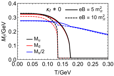
Figure 9: Dynamical masses as functions of the temperature for $u$ quark (black lines), $d$ quark (red lines), and $s$ quark (blue lines) with AMMs $\kappa_{f}\neq 0$ in magnetic fields $eB=5\,m_{\pi}^{2}$ (solid lines) and $eB=10\,m_{\pi}^{2}$ (dashed lines).

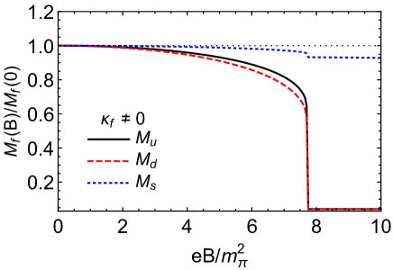
Figure 10: Dynamical masses as functions of the magnetic field strength at $T=150$ MeV for quarks with nonvanishing AMMs, normalized by masses when $eB=0$. Dynamical masses for $u$, $d$, and $s$ quarks are plotted with black solid line, red dashed line, and blue dotted line, respectively.

We plot in Fig. 9 dynamical masses as functions of the temperature for $u$, $d$, and $s$ quarks with $\kappa_{f}\neq 0$. As $T$ increases, masses of $u$ and $d$ quarks sharply decrease to their current masses, indicating a first-order phase transition that happens at $176$ MeV when $eB=5\,m_{\pi}^{2}$, and at $133$ MeV when $eB=10\,m_{\pi}^{2}$. Such a behaviour is significantly different from the cross-over in Fig. 1, indicating that the phase structure for light quarks are strongly affected by AMMs. On the other hand, the $s$ quark is less affected by the AMM and still undergoes a cross-over. In the chiral symmetry breaking phase, the quark masses at $eB=5\,m_{\pi}^{2}$ is larger than those at $eB=10\,m_{\pi}^{2}$, which is the inverse magnetic catalysis phenomena. The dependence to the magnetic field strength is shown in Fig. 10. We observe that the nonzero AMMs result in the inverse magnetic catalysis, i.e., the dynamical masses decrease with an increasing field strength, which is opposite to the case with $\kappa_{f}=0$ as shown in Fig. 2. Moreover, at a particular field strength, $M_{u}$ and $M_{d}$ suffer a discontinuity, corresponding to a first-order phase transition. For the set of AMMs in Eq. (34), the critical field strength is $eB_{C}=7.75\,m_{\pi}^{2}$ at $T=150$ MeV. Above this $eB_{C}$, dynamical masses for $u$ and $d$ quarks are consistent with current quark masses.

V.2 Spectral function for $\phi$ mesons

The propagator for vector meson is derived by solving the Dyson-Schwinger equation (10) with self-energy (11). In the presence of AMMs, the quark propagator is given by the following form,

$$S_{f}(p)=ie^{-p_{\perp}^{2}/|q_{f}B|}\sum_{n=0}^{\infty}(-1)^{n}D_{n}^{f}(p)\frac{1}{\mathcal{M}(p)-2n|q_{f}B|}\,,$$ (36)

where $D_{n}^{f}(p)$ is given by Eq. (13) with $M_{f}$ replaced by $M_{f}+i\kappa_{f}q_{f}B\gamma^{1}\gamma^{2}$. The explicit form of the matrix $\mathcal{M}$ is given in Ref. (Miransky and Shovkovy, 2015), from which we derive

$$\frac{1}{\mathcal{M}(p)-2n|q_{f}B|} =\frac{1}{U_{n}}\left[(p^{0})^{2}-(p_{z})^{2}-M_{f}^{2}-2n|q_{f}B|\right.$$

$$\left.\!\!\!\!\!\!\!\!\!\!\!\!\!\!+(\kappa_{f}q_{f}B)^{2}+2\kappa_{f}q_{f}B(p_{z}\gamma^{0}\gamma^{5}-p^{0}\gamma^{3}\gamma^{5})\right]\,,$$ (37)

where the denominator $U_{n}$ is given by

$$U_{n} = \left[(p^{0})^{2}-(p_{z})^{2}-M_{f}^{2}-2n|q_{f}B|-(\kappa_{f}q_{f}B)^{2}\right]^{2}$$ (38)

$$-4(M_{f}^{2}+2n|q_{f}B|)(\kappa_{f}q_{f}B)^{2}\,.$$

We note that the eigenenergies in Eq. (35) are determined by solutions of $U_{n}=0$. One can also prove that the propagator reduce to Eq. (12) in the absence of $\kappa_{f}$. Using the quark propagator and the dynamical mass obtained in the previous subsection, we are then able to calculate the vector meson’s spectral function. We still focus on the $\phi$ meson at static, ${\bf k={\bf 0}}$. The spectral functions at $T=100$ MeV, $150$ MeV, and 200 MeV are shown in Fig. 11. The magnetic field strength is set to $eB=5\,m_{\pi}^{2}$, leading to the difference between longitudinally $(\lambda=0)$ and transversely $(\lambda=\pm 1)$ polarized states. We also observe the bound state with $\lambda=0$ vanishes for all three considered temperatures, while bound states with $\lambda=\pm 1$ vanish at $T=250$ MeV and exist at $T=100$ MeV or $150$ MeV. The temperature dependence for the peak masses are shown in Fig. (12), where we observe that the bound state with $\lambda=0$ does not exist even at lower temperatures. Compared Fig. 12 with Fig. 5, we find that the $\lambda=\pm 1$ states and the resonance masses are nearly not affected by the AMMs. We also plot in Fig. 13 the $\phi$ meson masses as functions of magnetic field strength. When $eB<2.9\,m_{\pi}^{2}$, masses for bound states decrease in larger magnetic fields. The bound state with $\lambda=0$ suddenly increases approach the mass of the resonance state at $eB\sim 2.9\,m_{\pi}^{2}$ and then dissociate when $eB\gtrsim 3.4\,m_{\pi}^{2}$, corresponding to the Mott transition. The masses for resonance excitations are nearly independent to the AMMs, as compared to Fig. 6.

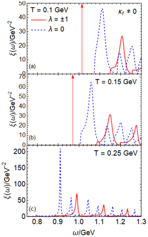
Figure 11: Spectral functions for $\phi$ mesons in a constant magnetic field with $eB=5m_{\pi}^{2}$, at $T=100$ MeV [panels (a)], $T=150$ MeV [panels (b)], and $T=250$ MeV [panels (c)]. The AMMs are set to nonzero values given in Eq. (34). Here red solid lines denote spectral functions for $\phi$ mesons with spin state $\lambda=\pm 1$ and blue dashed lines denote the spectral function of $\lambda=0$. Red and blue arrows correspond to delta functions.

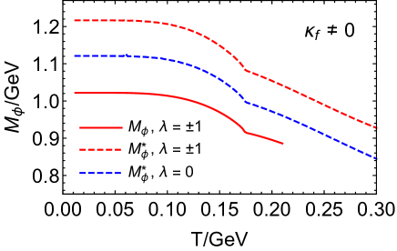
Figure 12: Dynamical masses as functions of the temperature for $\phi$ mesons at $eB=5\,m_{\pi}^{2}$. Masses for bound states with spin $\lambda=0$ and $\lambda=\pm 1$ are plotted with red solid lines and blue solid lines, respectively, while those for resonance excitations are plotted with red dashed lines and blue dashed lines, respectively. The AMMs for quarks are nonzero values given in Eq. (34).

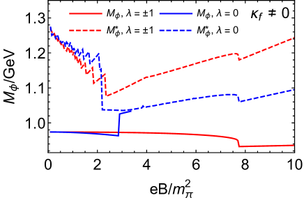
Figure 13: Dynamical masses as functions of $eB$ for $\phi$ mesons at $T=150$ MeV. Notations are the same as in Fig. 5.

V.3 Spin alignment for $\phi$ mesons

Substituting the spectral functions into Eqs. (22) and (24), we derive the $\phi$ meson’s spin alignment. For the case with nonzero AMMs, the spin alignments as functions of temperature and magnetic field strength are shown in Figs. 14 and 15, respectively. As a comparison, we also show results from a non-relativistic coalescence model (Yang et al., 2018), given by Eq. (32), with the magnetic moment $\mu_{s}=(1+2M_{s}\kappa_{s})q_{s}/(2M_{s})$ including the effect of AMM. From Fig. 14 we observe that the spin alignment for bound states is always equal to zero because all bound states have $\lambda=\pm 1$, as indicated by Fig. 12. The resonance states still have $\rho_{00}>\rho_{00}^{\text{Non-rel. coal.}}>1/3$, which is similar to the case with $\kappa_{f}=0$. On the other hand, in a weak magnetic field with $eB<2.5\,m_{\pi}^{2}$, $\rho_{00}$ for bound states still agrees well with the non-relativistic model. It jumps to a negative value at $eB\sim 2.9\,m_{\pi}^{2}$, which is a straightforward result of the Mott transition for states with $\lambda=0$. When the magnetic field strength $eB\gtrsim 3.4\,m_{\pi}^{2}$, the bound state with $\lambda=0$ dissociates in the thermal medium, resulting in a vanishing spin alignment $\rho_{00}=0$. Meanwhile, the $\rho_{00}$ for resonance excitations shows a non-monotonic structure: $\rho_{00}<1/3$ when $eB<2.6\,m_{\pi}^{2}$ and $\rho_{00}>1/3$ when $eB>2.6\,m_{\pi}^{2}$.

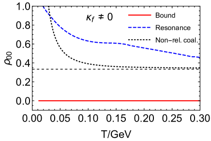
Figure 14: Spin alignments as functions of the temperature. The magnetic field strength is taken as $eB=5\,m_{\pi}^{2}$. The quark AMMs are set to nonzero values given in Eq. (34).

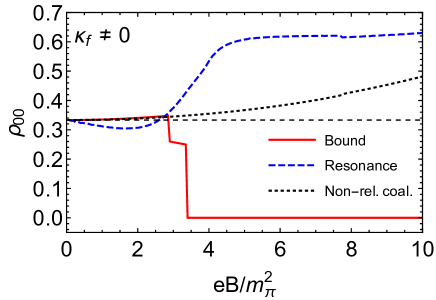
Figure 15: Spin alignments as functions of the magnetic field strength at temperature $T=150$ MeV. Notations are the same as in Fig. 7.

VI Summary

In this manuscript, we study the mass splitting and the spin alignment for the vector $\phi$ meson in a hot magnetized matter. The three-flavor NJL model is used to properly include the chiral phase transition. In this framework, mesons are described as quantum fluctuations beyond the mean-field background. The meson’s propagator is given by resuming quark bubbles at the random phase approximation. For a vector meson, the propagator is a Lorentz tensor perpendicular to the meson’s momentum, which can be further projected into the spin space. The spin density matrix is then derived by the convolution of the spectral function and the Bose-Einstein distribution, while the spectral function is given by the imaginary part of the propagator. In this way, we are able to calculate the vector meson’s spin alignment in a thermal medium.

If we choose the spin quantization direction for the vector meson as the direction of the external magnetic field, the density matrix is then diagonal and spin states $\lambda=\pm 1$ are degenerate. We numerically calculated the spectral functions for $\phi$ mesons. In general the spectral function can be separated into a delta-function part corresponding to a quark-antiquark bound state, and a continuum part corresponding to resonance excitations. We observe multi-peak structures in the continuum part, which is the result of Landau quantization for constituent quarks. The magnetic field leads to a mass splitting between states with $\lambda=0$ and $\lambda=\pm 1$, resulting in the spin alignment $\rho_{00}\neq 1/3$ for the $\phi$ meson in a hot medium. If we only focus on the bound states, we find that $\rho_{00}>1/3$ and is in good agreement with the result from the non-relativistic coalescence model. However, the spin alignment for resonance states gives a much larger result.

Since constituent quarks and free quarks have different magnetic moments, we incorporate the quark AMMs according to the constituent quark magnetic moments observed in experiments. The light-flavor quarks then show the inverse magnetic catalysis behaviors, and the chiral phase transition is first order. The AMMs then significantly modify the mass spectra and the spin alignment for the $\phi$ meson, especially in a strong magnetic field. Considering a different choice of AMMs, like in Ref. (Kawaguchi and Huang, 2022), may result in a different $\rho_{00}$, which is waiting for more comprehensive studies in the future.

Even though the spin quantization direction is fixed to the direction of the magnetic field in our numerical calculations, we can easily generalize the results to the case that $\rho_{00}$ is measured along any other direction, c.f., Eq. (29). This is achieved by performing a rotation in spin space for the density matrix. Therefore results in this work can be applied to study the $\phi$ meson’s spin alignment in a fluctuating magnetic field. When the fluctuation is anisotropic in space, the spin alignment $\rho_{00}$ will deviate from $1/3$. Therefore this work may help us better understand the role of the magnetic field in the $\phi$ mesons’ spin alignment.