Unsupervised Domain Adaptation
via Style-Aware Self-intermediate Domain

Abstract

Unsupervised domain adaptation (UDA) has attracted considerable attention, which transfers knowledge from a label-rich source domain to a related but unlabeled target domain. Reducing inter-domain differences has always been a crucial factor to improve performance in UDA, especially for tasks where there is a large gap between source and target domains. To this end, we propose a novel style-aware feature fusion method (SAFF) to bridge the large domain gap and transfer knowledge while alleviating the loss of class-discriminative information. Inspired by the human transitive inference and learning ability, a novel style-aware self-intermediate domain (SSID) is investigated to link two seemingly unrelated concepts through a series of intermediate auxiliary synthesized concepts. Specifically, we propose a novel learning strategy of SSID, which selects samples from both source and target domains as anchors, and then randomly fuses the object and style features of these anchors to generate labeled and style-rich intermediate auxiliary features for knowledge transfer. Moreover, we design an external memory bank to store and update specified labeled features to obtain stable class features and class-wise style features. Based on the proposed memory bank, the intra- and inter-domain loss functions are designed to improve the class recognition ability and feature compatibility, respectively. Meanwhile, we simulate the rich latent feature space of SSID by infinite sampling and the convergence of the loss function by mathematical theory. Finally, we conduct comprehensive experiments on commonly used domain adaptive benchmarks to evaluate the proposed SAFF, and the experimental results show that the proposed SAFF can be easily combined with different backbone networks and obtain better performance as a plug-in-plug-out module.

1 Introduction

Deep neural networks have achieved remarkable achievements in various machine learning fields, including image classification [1, 2], semantic segmentation [3], and object recognition [4]. However, recent achievements heavily relied on large-scale datasets under the major assumption that the training and testing data have a consistent feature distribution. While in practice, the data collected from various scenes may suffer from different lighting conditions, color saturation, hue, visual angles, and background environments, resulting in domain gaps between training and testing data. Aiming at the above problems, domain adaptation can map data from different distributions of source and target domains into a feature space, and optimize the corresponding model parameters to make the distance of features from different domains as close as possible in this space. According to the existence of labels in the target domain, domain adaptation can be divided into supervised domain adaptation, semi-supervised domain adaptation and unsupervised domain adaptation (UDA) [5]. Since data labeling is often time-consuming, labor-intensive, and expensive, obtaining high-quality labels has always been an important factor limiting performance improvement. Compared with supervised and semi-supervised methods, UDA does not require any labeled target domain data and has more potential application scenarios, which deserves further attention. Therefore, in this paper, we focus on exploring UDA method aiming to transfer knowledge from a labeled source domain to a different unlabeled target domain.

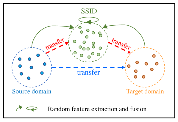
Figure 1: The illustration of the proposed SSID. The large gap between the source and target domains (indicated by the blue dashed line) adds to the challenge of class-discriminative information transfer in UDA task. The proposed SSID learning strategy randomly extracts samples from multiple domains as anchors, and computes their object and style features. Then a labeled intermediate auxiliary class-discriminative information is generated by randomly fusing the object and style features for knowledge transferring (indicated by the red dashed line). Finally, the labeled and style-rich SSID could act as a bridge to implicitly transfer class information from the source to the target domains.

Over the past few years, many UDA methods have emerged, which can be roughly categorized as two types: 1) difference-based methods [6, 7, 8, 9, 10, 11, 12, 13, 14, 15], which explicitly mitigate inter-domain difference by minimizing statistical metrics such as maximum mean discrepancy, joint maximum mean discrepancy, margin disparity discrepancy, and optimal transport distance; and 2) adversarial-based methods [16, 17, 18, 19], which introduce a discriminator to adversarially learn domain-invariant representations by obfuscating domain-specific information. These methods devote to strengthening the feature transferability between domains to alleviate the problem of inter-domain differences. However, under the UDA conditions, for the former, the feature extractor may incorrectly draw the distance of different classes closer, resulting in a decline in class recognition ability, i.e. a decrease in discriminability; for the latter, the discriminator forces the feature extractor to learn domain-invariant representations, while ignoring the learning of class-variant representations, which may also lead to a decline in discriminability. This decline in discriminability is ineviTable. Since the target domain is completely unlabeled, when the domain gap is large, the class-discriminative information is easily lost when performing domain alignment, and the classifier remains inevitably biased towards the source domain [18, 20], leading to unexpected deterioration of discriminability in the target domain. Based on the above observations, our work focuses on designing a more robust solution to simultaneously enhance feature transferability and discriminability to further reduce the domain gap.

Inspired by the human transitive inference and learning ability [21], we investigate a novel domain adaptation method: style-aware self-intermediate domain (SSID), where two seemingly un-overlapping domains can be linked through a series of intermediate auxiliary synthesis concepts. Specifically, the source and target domains are distinguished mainly by their image styles, such as lighting conditions, color saturation, hue, visual angle, background environment, etc. When the styles of the same class are quite different, incorrect feature alignment will occur and the discriminability of the target domain will also be sacrificed. Therefore, we consider generating labeled and style-rich auxiliary intermediate features to connect the source and target domains. Based on this, as in Fig. 1, the learning strategy of SSID is to randomly extract features from multiple domains as anchors, and compute their object and style features. And then the labeled auxiliary class-discriminative information is synthesized by randomly fusing the object and style features. Therefore, labeled and style-rich SSID can act as a bridge to implicitly transfer domain information from the source to the target domain. Moreover, we also introduce an external memory bank with six memory cells to store the specified features of the SSID and the source domain. The feature centers are calculated and stored through the labels of the source domain data to obtain sTable class features and class-wise style features. Based on the proposed memory bank, we further design novel intra- and inter-domain losses for SAFF to improve the class recognition ability and feature compatibility, respectively. We simulate the rich latent feature space of SSID through infinite sampling, deduce the upper bound loss function, and demonstrate the convergence of the proposed loss function.

In general, we highlight our four-fold contributions:

• In this paper, we propose a novel UDA solution, named style-aware feature fusion (SAFF), to bridge the large gap between domains and transfer knowledge while alleviating the loss of class-discriminative information. Meanwhile, a novel style-aware self-intermediate domain (SSID) is also designed to generate labeled and style-rich auxiliary intermediate features by style-aware extraction and fusion, implicitly narrowing the gap between the source and target domains.

• An external memory bank is introduced to store specified features based on the sample index and then calculate their class centers for the subsequent computation.

• Develop the novel intra- and inter-domain losses for the SAFF to improve the class recognition ability and feature compatibility of the network respectively. Besides, we simulate the rich latent feature space of SSID by infinite sampling and demonstrate the convergence of the proposed loss function for the first time.

• Conduct extensive experiments on commonly used domain adaptive benchmarks to validate the proposed method. The experimental results show that, as a plug-in-plug-out technique, SAFF can be easily applied to various UDA backbones and achieves the best performances, including 84.86$\%$ on Office-Home and 85.40$\%$ on VisDA-2017.

2 RELATED WORK

UDA has attracted increasing attention in the deep learning community, aiming to minimize distribution differences between different but related domains. Recently, many UDA methods have been proposed and successfully applied in cross-domain applications. Existing UDA methods could be mainly divided into two categories, difference-based UDA and adversarial-based UDA.

2.1 Difference-Based UDA Method

Difference-based UDA alleviates domain differences by minimizing statistical differences. [6] minimized the maximum mean difference for task-specific layers to explicitly narrow the domain gap. [7] introduced joint maximum mean difference to enforce joint distribution alignment between domains. [8] and [9] minimized inter-domain differences by aligning the second-order statistics of the source and target distributions. Based on the optimal transfer distance, [10, 11, 12, 13] designed optimal transfer models to perform feature alignment in source and target domains. Regularizes such as entropy constraints [14] or maximum prediction rank [15] can be used to implicitly constrain the cross-domain feature space. Although such methods help to narrow the distance of similar features between domains, due to the lack of labels in the target domain, the feature extractor may incorrectly draw the distance of similar but non-same-class features, resulting in a decrease in discriminability.

2.2 Adversarial-Based UDA Method

Adversarial-based UDA introduces a discriminator to adversarially learn domain-invariant representations by obfuscating domain-specific information. DANN [16] introduced a gradient inversion layer and a domain discriminator to confuse the feature distributions of the two domains. CDAN [17] further introduced categorical information entropy into the domain discriminator to alleviate the class mismatch problem. In order to maintain the inter-class discriminativeness while confusing the domain feature distribution, [18] proposed a penalty method for penalizing the largest singular value. [19] adopted a new adversarial paradigm, where the adversarial way occurs between the feature extractor and the classifier, rather than between the feature extractor and the domain discriminator. Such methods take the features within a domain as a whole and force the feature extractor to learn domain-invariant representation by confusing the domain discriminator. However, finer intra-domain information, such as class-specific features may be confused, thus reducing the discriminability.

2.3 Other UDA Method

Furthermore, some works exploit pseudo labels for target domain data [26, 27, 28], and take them as labeled data to refine the model. Their success partly depends on the quality of the pseudo-labels obtained during the preprocessing step. Through the marginal sampling algorithm, [29] collected and labeled a small number of representative samples of the target domain, and explicitly further optimizes and generalizes the decision boundary to the target distribution. However, professionals are required to label the samples multiple times during training.

Other line of traditional methods [30, 31] tried to embed the source and target data into a Grassmann manifold and learn a specific geodesic path between the two domains to bridge the source and target domains, but they are not easily applicable to deep model. Following them, [32] proposed a person re-identification method based on the shortest geodesic path definition, forcing the positioning of the intermediate domain on the appropriate path between the source and target domains in the manifold, but their method is designed for supervised domain adaptation since their bridging loss involves labels from the target-train set. [33] proposed a GAN-based source domain-like target domain image, but it is computationally expensive and GAN-based methods may cause mode collapse. [34] proposed a transferable semantic augmentation approach to enhance the classifier adaptation ability, but missed the feature admixture association between different categories.

Recently, some Transformer-based UDA explorations [35, 36, 37] have been reported. CDTrans [35] provides one of the first attempts to solve UDA tasks with a pure transformer solution, and it applies cross attention on source-target image pairs, However, it ignores the cross-attention from the target domain to the source domain. TransDA [36] considers the source-free domain adaptation task and proposes a novel self-supervised knowledge distillation approach with target pseudo-labels, but it focuses on extracting object features and weakens useful style features. [37] leverage class token and discriminative clustering to enhance feature diversity and separation which are undermined during adversarial domain alignment. However, its number parameters are large and only suiTable for Transformer-based networks Our method differs in that it not only considers the transfer from the source domain to the target domain, but also generates a labeled, style-rich SSID as a bridge between the source and target domains through random fusion for implicitly transferring class-discriminative information. Therefore, transferability and discriminability can be improved simultaneously.

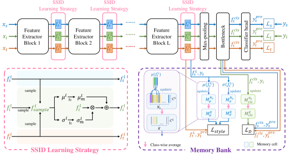
Figure 2: The illustration of our proposed SAFF, including the SSID learning strategy, the external memory bank, and intra/inter-domain losses. The samples from the source domain, SSID, and target domain are fed into the feature extractor in parallel, denoted by blue, green, and orange, respectively. The SSID is deployed after each feature extractor block, while the external memory bank is designed to store specified labeled features to obtain sTable class features and class-wise style features for subsequent computation.

3 Methodology

In this section, we detail each part of our proposed SAFF, which aims to develop a solution that can both improve the transferability of cross-domain features and exploit class-discriminative information to generate labeled cross-domain representations that implicitly preserve class-discriminative information, thereby further narrowing the domain gap in UDA. Fig. 2 illustrates our proposed SAFF. $x_{s}$, $x_{i}$ and $x_{t}$ are samples from source domain $S=\left\{{\left({{x_{sm}},{y_{sm}}}\right)}\right\}_{m=1}^{{N_{s}}}$, SSID $I=\left\{{\left({{x_{in}},{y_{in}}}\right)}\right\}_{n=1}^{{N_{s}}}$ and target domain $T=\left\{{\left({{x_{tp}}}\right)}\right\}_{p=1}^{{N_{t}}}$ respectively, which are fed into the feature extractor in parallel, and $I$ is initialized by $S$. Where $y\in\left\{{1,2,\ldots,K}\right\}$ is the label of $x$, $N$ and $K$ denote the number of sample and class respectively. The Vision Transformer (ViT) [38, 39] is used as the feature extractor to extract more general representations as its outstanding performance in many computer vision tasks [40, 41]. Our feature extractor consists of $L$ feature extractor blocks followed by SSID learning strategy, which we described in detail in Section III. A. Then there is the max-pooling layer, the bottleneck layer, and the classifier head layer for classification. The specified output of the feature extractor and bottleneck layer are stored and updated in the external memory bank for subsequent loss function computation. The memory bank and loss functions are introduced in Sections III. B and III. C, respectively.

3.1 Style-aware Self-Intermediate Domain (SSID) Learning Strategy

Style refers to a series of weak semantically related cues in the feature map, such as lighting conditions, hue, color saturation, background environment, etc. Samples from different domains have large stylistic differences, which leads to an increase in the difficulty of UDA tasks. Most of the previous UDA work is devoted to improving the feature transferability of different domains, that is, suppressing the weak style-related feature that appears to be a distractor. But this suppression also inevitably leads to the loss of fine class-discriminative features, while the model should rely on richer cues to become robust. Therefore, instead, we improve the robustness of the model by enriching cross-domain style information.

Style transfer practices have conjectured that styles are homogeneous, consisting of repeated structural motifs. Two images are similar in style if the features extracted by a trained classifier share the same statistics [42, 43], such as first- and second-order statistics, which are used due to their computational efficiency. The first- and second-order statistics refer to the mean and variance of the extracted features, which are called style features. Object features refer to pure semantic information without style information. Similar to [44], the object features $f_{o}$ can be obtained by cleaning style features as:

$$f_{o}=\frac{{f_{c}-{\mu(f_{c})}}}{{{\sigma(f_{c})}}},$$ (1)

where $\mu(f_{c})$ and $\sigma(f_{c})$ denote the mean and variance of extracted feature $f_{c}$. Furthermore, style can be re-assign by $f_{o}\cdot\gamma+\beta$, where $\gamma$ and $\beta$ are learned parameters. Afterward, [42] further explored adapting $f_{o}$ to arbitrarily given style by using style features of another extracted feature instead of learned parameters. Inspired by them, we design a feature fusion method as shown in Fig. 3, and applied it to the UDA task. First, the input images are divided into content images and style images, and their features extracted by a trained classifier are denoted as $f_{c}$ and $f_{s}$, respectively. Secondly, the style features $\mu(f_{c})$ and $\sigma(f_{c})$ of content images are cleaned to obtain the object features $f_{o}$. Thirdly, the styles of style images are re-assigned to $f_{o}$ to obtain fused features $f_{c\rightarrow s}$. Based on these, the content and style of $f_{c\rightarrow s}$ are consistent with the content images and style images respectively. The feature fusion method aims to generate another style of features for the class in the content images, thereby enriching the distribution of that class in the feature space.

We extend the above feature fusion method and design the learning strategy of SSID: randomly sample and fuse features from different domains to generate labeled, style-rich features to enrich the feature space of each class, so as to implicitly transfer class-discriminative information from the source to the target domain.

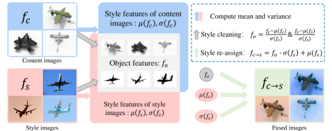
Figure 3: The illustration of style fusion from content images to style images. Style features of the style images are used to perform style re-assign on the object features of the content images to obtain the fused features. The content and style of the fused images are consistent with the content images and the style images, respectively. Features can be visualized by a trained generator.

As shown in Fig. 2, SSID learning strategy is appended to each feature extractor block. The input feature maps of the $l$-th learning strategy in source domain, SSID and target domain are $f_{s}^{l}$, $f_{i}^{l}$, and $f_{t}^{l}\in{\mathbb{R}^{B\times N\times{C^{l}}}}$ respectively, where $B$ represents the batch size, $N$ represent the window size and ${C^{l}}$ is the output feature dimension in this block. In the SSID learning strategy, we first randomly sample the feature maps of the three domains at a one-third scale to obtain feature maps $f_{sample}^{l}\in{\mathbb{R}^{B\times N\times{C^{l}}}}$. Then calculate its channel-wise mean $\mu^{l}\in{\mathbb{R}^{B\times{C^{l}}}}$ and variance $\sigma^{l}\in{\mathbb{R}^{B\times{C^{l}}}}$ as style features.

To avoid the overflow caused by the small divisor in Eq. (1), two fully connected layers $FC$ are applied to linearly transform ${\mu^{l}}$ and ${\sigma^{l}}$, and the above feature fusion process is modified as:

$$f_{i}^{l}\leftarrow(f_{i}^{l}\bigotimes FC(\sigma^{l}))\bigoplus FC(\mu^{l}),$$ (2)

where $\bigotimes$ and $\bigoplus$ represent channel multiplication and addition, respectively. Since we discard the object features and only use the style features of $f_{sample}^{l}$, the semantic information and labels of $f_{i}^{l}$ are preserved. Through continuous feature fusion, SSID can build a labeled, style-rich latent feature space for each class, so as to implicitly transfer class-discriminative information from the source to the target domain.

3.2 Memory Bank

In our method, we utilize an external memory bank with six memory cells to store the specified features of the SSID and the source domain in real time during training via index. These features are then applied to calculate sTable class features and class-wise style features for downstream computing tasks, as shown in Fig. 2. In this section, we detailed the workflow of our proposed memory bank.

3.2.1 Initialization Strategy of Memory Bank

Before training, the pre-trained feature extractor with frozen model parameters is utilized to initialize the memory bank as follows:

• Since the output feature maps of the feature extractor $F^{L}=\left[f_{s}^{L},f_{i}^{L},f_{t}^{L}\right]$ contains rich semantic information with style clues, and feature vector $F^{cls}=\left[f_{s}^{cls},f_{i}^{cls},f_{t}^{cls}\right]$ before the classifier head layer contains refined class-discriminative information, we store $f_{s}^{L}\in{\mathbb{R}^{B\times N\times{C^{L}}}}$ and $f_{i}^{cls}\in{\mathbb{R}^{B\times{C^{cls}}}}$ in the memory bank, where $C^{L}$ and $C^{cls}$ denote the output feature dimension of feature extractor and bottleneck layer.

• Calculate the channel-wise mean $\mu\left({f_{s}^{L}}\right)\in{\mathbb{R}^{B\times{C^{L}}}}$ and variance $\sigma\left({f_{s}^{L}}\right)\in{\mathbb{R}^{B\times{C^{L}}}}$ of $f_{s}^{L}$, and update the corresponding $B$ features in memory cells $M_{\mu}^{{N_{s}}}\in{\mathbb{R}^{{N_{s}}\times{C^{L}}}}$ and $M_{\sigma}^{{N_{s}}}\in{\mathbb{R}^{{N_{s}}\times{C^{L}}}}$ according to the sample index. Meanwhile, $M_{cls}^{{N_{s}}}\in{\mathbb{R}^{{N_{s}}\times{C^{cls}}}}$ is updated with $f_{i}^{cls}$ according to the sample index.

• Repeat the above steps until all samples in $S$ and $I$ have been traversed. Calculate the class centers of all features in $\left\{{M_{\mu}^{{N_{s}}},M_{\sigma}^{{N_{s}}},M_{cls}^{{N_{s}}}}\right\}$ according to their class labels and store the result in $\left\{{M_{\mu}^{K}\in{\mathbb{R}^{K\times{C^{L}}}},M_{\sigma}^{K}\in{\mathbb{R}^{K\times{C^{L}}}},M_{cls}^{K}\in{\mathbb{R}^{K\times{C^{cls}}}}}\right\}$, respective. Finally, unfreeze the model parameters.

3.2.2 Update Strategy of Memory Bank

During training, we directly discard those obsolete features $f_{s}^{L}$ and $f_{i}^{cls}$ according to the index of the samples and replace them with the latest features, then calculate and update the corresponding features in six memory cells $\left\{{M_{\mu}^{{N_{s}}},M_{\sigma}^{{N_{s}}},M_{cls}^{{N_{s}}},M_{\mu}^{K},M_{\sigma}^{K},M_{cls}^{K}}\right\}$ as in the initialization strategy. Among them, $M_{cls}^{K}$ stores $K$ class features, while $M_{\mu}^{K}$ and $M_{\sigma}^{K}$ store style features of $K$ classes, which are used for downstream computation. Furthermore, the proposed memory bank is only an external repository and does not participate in the back-propagation calculation of the network.

3.3 Loss Function

Based on the designed memory bank, we proposed a novel joint loss function which integrates the intra-domain loss ${{\cal L}_{intra}}$ and inter-domain loss ${{\cal L}_{inter}}$ to improve the class recognition ability and feature compatibility, respectively. The overall loss function $\cal L$ is as follows:

$${\cal L}={{\cal L}_{intra}}+\alpha\cdot{{\cal L}_{inter}},$$ (3)

where $\alpha$ is a hyperparameter with a default value of 1.0 to balance ${{\cal L}_{intra}}$ and ${{\cal L}_{inter}}$.

3.3.1 Intra-domain Loss Function

Intra-domain loss function ${{\cal L}_{intra}}$ is designed to improve the class recognition ability, which consists of the respective domain loss functions of the source domain ${{\cal L}_{s}}$, style-aware self-intermediate domain ${{\cal L}_{i}}$ and target domain ${{\cal L}_{t}}$, as:

$${{\cal L}_{intra}}={{\cal L}_{s}}+{{\cal L}_{i}}+{{\cal L}_{t}}.$$ (4)

For the labeled source domain and SSID, the network can be trained with the traditional cross-entropy loss function:

$${{\cal L}_{s}}={{\cal L}_{CE}}\left({y_{s}^{pre},{y_{s}}}\right),$$ (5)

$${{\cal L}_{i}}={{\cal L}_{CE}}\left({y_{i}^{pre},{y_{i}}}\right),$$ (6)

where ${\cal L}_{CE}$ represent the cross-entropy loss function, $y^{pre}$ and $y$ denote the predicted result by classifier head layer and the ground truth, respectively. Meanwhile, mutual information maximization is employed on the unlabeled target domain, as:

$${{\cal L}_{t}}=\frac{1}{{{N_{t}}}}\sum\limits_{p=1}^{{N_{t}}}{\sum\limits_{k=1}^{K}{y_{tpc}^{pre}}}\log(y_{tpc}^{pre})-\sum\limits_{k=1}^{K}{y_{tc}^{pre}\log(y_{tc}^{pre})},$$ (7)

where $y_{tpc}^{pre}$ denotes the probability that the $p$-th sample in the target domain is predicted to be the $c$-th class, and $y_{tc}^{pre}=\sum\limits_{p=1}^{{N_{t}}}{y_{tc}^{pre}}$.

3.3.2 Inter-domain Loss Function

Inter-domain loss function ${{\cal L}_{inter}}$ consists of discrimination loss function ${{\cal L}_{D}}$ and style loss function ${{\cal L}_{style}}$, as:

$${{\cal L}_{inter}}={{\cal L}_{D}}+{{\cal L}_{style}}.$$ (8)

To maintain the consistency of the class features of the source domain $\&$ SSID and the target domain $\&$ SSID to improve the discriminability, we design a discrimination loss function ${\cal L}_{D}$, as:

$${{\cal L}_{D}}=KL(M_{cls}^{K}[y_{s}^{pre}]||f_{s}^{cls})+KL(M_{cls}^{K}[y_{t}^{pre}]||f_{t}^{cls}),$$ (9)

where $f_{s}^{cls}$ and $f_{t}^{cls}$ represent the real-time feature vectors of the source domain and the target domain before the classifier head layer in the current iteration, respectively. $M_{cls}^{K}[y^{pre}]$ represents the class center of $y^{pre}$ stored in memory cell $M_{cls}^{K}$, and $KL$ stands for Kullback–Leibler divergence.

Style loss function ${{\cal L}_{style}}$ aims to reduce the difference of class-wise style features in the source and target domain to improve inter-domain transferability, as:

$${{\cal L}_{style}}={up_{rate}}\cdot KL(M_{\mu}^{K}[y_{t}^{pre}]||\mu(f_{t}^{L}))$$ (10)

$$\quad\quad\quad+KL(M_{\sigma}^{K}[y_{t}^{pre}]||\mu(f_{t}^{L})),$$

where $M_{\mu}^{K}[y_{t}^{pre}]$ and $M_{\sigma}^{K}[y_{t}^{pre}]$ represents the style features of $y_{t}^{pre}$ stored in memory cell $M_{\mu}^{K}$ and $M_{\sigma}^{K}$ respectively. $f_{t}^{L}$ denotes the feature maps of the target domain output by the feature extractor in the current iteration, $\mu(\cdot)$ and $\sigma(\cdot)$ denote mean and variance operations, respectively. Furthermore, since the style features in the early stage of the network are not robust enough, we introduced a rising factor $u{p_{rate}}={\left({\frac{{epoch\_num}}{{total\_epoch}}}\right)^{rate}}$, where $rate$ is set to 0.9.

3.3.3 Convergence Analysis of Loss Function

The convergence of the loss function is a crucial necessary condition for calculating the optimal network parameters. With a limited number of samples, it is easy to infer that the cross-entropy loss function and the mutual information maximization function are convergent, that is, ${\cal L}_{s}$, ${\cal L}_{t}$, ${\cal L}_{D}$ and ${\cal L}_{style}$ are all convergent. Therefore, in this section, we focus on proving the convergence of ${\cal L}_{i}$. The expansion of ${\cal L}_{i}$ is as follows:

$${\cal L}_{i}=\frac{1}{N_{s}}\sum\limits_{n=1}^{N_{s}}\frac{1}{N_{i}}\sum\limits_{m=1}^{N_{i}}{-y_{in}\log(y_{in\rightarrow m}^{pre})},$$ (11)

where $N_{i}$ denotes the number of features in the latent feature space of SSID. $y_{in}$ and $y_{in\rightarrow m}^{pre}$ represent the ground truth of the $n$-th input sample and the prediction result of the $m$-th feature fusion of the n-th sample, respectively.

From a statistical point of view, the latent feature space of SSID is huge. At each iteration, the mini-batch of each domain is randomly selected, a total ${\left({C_{{N_{s}}}^{B}}\right)^{2}}C_{{N_{t}}}^{B}{({A_{B}^{B/3}})^{3}}$ features can be obtained after one layer of SSID learning strategy. After $L$ layers, the number of features ${N_{i}}$ in the latent feature space will reach an amazing value. Since it is nearly impossible to traverse all features in the latent feature space of the SSID, the real number $N_{i}$ is approximately replaced by the sampling number $M$.

Assuming that the feature of each class in each domain obeys a normal distribution $N(\mu_{d}^{k},\sigma_{d}^{k})$ , where $k$ denote the class number, and $d$ takes the value from $\left[s,i,t\right]$. For the input sample $(x_{in},y_{in})$ in SSID, its fused feature before classifier head layer is noted as $\widehat{f_{in\rightarrow 1}^{{y_{in}}}}$. After $M$ times sampling and fusion, an auxiliary synthesis feature set of $(x_{in},y_{in})$ will be obtained:

$$\left\{{\left({\widehat{f_{in\rightarrow 1}^{y_{in}}},y_{in}}\right),\left({\widehat{f_{in\rightarrow 2}^{y_{in}}},y_{in}}\right),\ldots,\left({\widehat{f_{in\rightarrow M}^{y_{in}}},y_{in}}\right)}\right\}.$$ (12)

Under the above condition, using the parameters of the classifier head layer and softmax to expand the predicted value $y_{in\rightarrow m}^{pre}$ of all input samples, then Eq. (11) can be rewritten as:

$${\cal L}_{i}\left({\theta,W,b}\right)=\frac{1}{N_{s}}\sum\limits_{n=1}^{N_{s}}\frac{1}{M}\sum\limits_{m=1}^{M}{-\log(\frac{{{e^{W_{{y_{in}}}^{T}\widehat{f_{in\rightarrow m}^{{y_{in}}}}+{b_{{y_{in}}}}}}}}{{\sum\limits_{k^{\prime}=1}^{K}{{e^{W_{k^{\prime}}^{T}\widehat{f_{in\rightarrow m}^{{y_{in}}}}+{b_{k^{\prime}}}}}}}})},$$ (13)

where $W$ and $b$ denote the weight matrix and bias vector of the classifier head layer respectively. Eq. (13) aims to reduce the difference between the predicted distribution and the actual distribution of features in the latent feature space of the SSID, so as to improve the classification performance of the network. Intuitively, the closer the value of $M$ is to $N_{i}$, the more robust the features in the latent space. Therefore, we need to explore whether ${\cal L}_{i}$ converges when the sampling times $M$ are continuously growing until infinity. When $M\rightarrow\infty$, Eq. (13) can be rewritten as:

$$\mathop{\lim}\limits_{M\to\infty}{{\cal L}_{i}}\left({\theta,W,b}\right)$$ (14)

$$=\frac{1}{{{N_{s}}}}\sum\limits_{n=1}^{{N_{s}}}{{E_{\widehat{f_{in\to m}^{{y_{in}}}}}}}\left[{-\log(\frac{{{e^{W_{{y_{in}}}^{T}\widehat{f_{in\to m}^{{y_{in}}}}+{b_{{y_{in}}}}}}}}{{\sum\limits_{k^{\prime}=1}^{K}{{e^{W_{k^{\prime}}^{T}\widehat{f_{in\to m}^{{y_{in}}}}+{b_{k^{\prime}}}}}}}})}\right]$$

$$=\frac{1}{{{N_{s}}}}\sum\limits_{n=1}^{{N_{s}}}{\sum\limits_{k=1}^{K}{\frac{{{N_{ik}}}}{{{N_{i}}}}}{E_{\widehat{f_{in}^{k}}}}[\log\left({\sum\limits_{k^{\prime}=1}^{K}{{e^{\left({W_{k^{\prime}}^{T}-W_{{y_{in}}}^{T}}\right)\widehat{f_{in}^{k}}+{b_{k^{\prime}}}-{b_{{y_{in}}}}}}}}\right)]},$$

where $\frac{N_{ik}}{N_{i}}$ denotes the proportion of the $k$-th class in the latent feature space, which is unknown but can be estimated statistically. According to the moment generating function and Jason’s inequality, the upper bound of Eq. (14) can be found as follows:

$$\mathop{\lim}\limits_{M\to\infty}{{\cal L}_{i}}\left({\theta,W,b}\right)$$ (15)

$$\leq\frac{1}{{{N_{s}}}}\sum\limits_{n=1}^{{N_{s}}}{\sum\limits_{k=1}^{K}{\frac{{{N_{ik}}}}{{{N_{i}}}}}\log\left({\sum\limits_{k^{\prime}=1}^{K}{{E_{\widehat{f_{in}^{k}}}}}\left[{{e^{W_{k^{\prime}y}\widehat{f_{in}^{k}}+B}}}\right]}\right)}$$

$$=\frac{1}{{{N_{s}}}}\sum\limits_{n=1}^{{N_{s}}}{\sum\limits_{k=1}^{K}{\frac{{{N_{ik}}}}{{{N_{i}}}}}\log\left({\sum\limits_{k^{\prime}=1}^{K}{{e^{W_{k^{\prime}y}\widehat{\mu_{in}^{k}}+B+\frac{1}{2}{W_{k^{\prime}y}^{T}}\widehat{\sigma_{in}^{k}}W_{k^{\prime}y}}}}}\right)}$$

$$=\frac{1}{{{N_{s}}}}\sum\limits_{n=1}^{{N_{s}}}{\sum\limits_{k=1}^{K}{\frac{{{N_{ik}}}}{{{N_{i}}}}}\left({-\log\left({\frac{{{e^{{A_{{y_{in}}}}}}}}{{\sum\limits_{k^{\prime}=1}^{K}{{e^{{A_{k^{\prime}y}}}}}}}}\right)}\right)},$$

where $W_{k^{\prime}y}=W_{k^{\prime}}^{T}-W_{{y_{in}}}^{T}$ and $B=B_{k^{\prime}}-b_{{y_{in}}}$, respectively. ${A_{{y_{in}}}}=W_{{y_{in}}}^{T}\widehat{\mu_{in}^{k}}+{b_{{y_{{}_{in}}}}}+\frac{1}{2}{(W_{{y_{in}}}^{T}-W_{{y_{in}}}^{T})^{T}}\widehat{\sigma_{in}^{k}}(W_{{y_{in}}}^{T}-W_{{y_{in}}}^{T})$ and ${A_{k^{\prime}}}=W_{k^{\prime}}^{T}\widehat{\mu_{in}^{k}}+{b_{k^{\prime}}}+\frac{1}{2}{(W_{k^{\prime}}^{T}-W_{{y_{in}}}^{T})^{T}}\widehat{\sigma_{in}^{k}}(W_{k^{\prime}}^{T}-W_{{y_{in}}}^{T})$ are polynomials related to $W_{y_{in}}^{T}$ and $W_{k^{\prime}}^{T}$.

Essentially, since the upper bound function Eq. (15) is a form of cross-entropy loss function, $\mathop{\lim}\limits_{M\to\infty}{L_{i}}\left({\theta,W,b}\right)$ is convergent and its performance is independent of the value of the sampling times $M$. Finally, we summarize the strategy of our proposed SAFF in Algorithm 1.

Algorithm 1 Style-aware Feature Fusion Method (SAFF).

0:  The source domain $S$, SSID $I$, the target domain $T$, number of feature extractor blocks $L$, and sampling number $M$.

1:  Initialize $I$ with $S$.

2:  Initialize the memory bank.

3:  For $epoch=1$ to $Maxepochs$ do

4:    For $l=1$ to $L$ do

5:      Calculate the output of $x_{s}$, $x_{i}$, $x_{t}$ in the $l$-th     feature extractor block: $f_{s}^{l}$, $f_{i}^{l}$, $f_{t}^{l}$.

6:      Randomly select $M/3$ features from $f_{s}^{l}$, $f_{i}^{l}$     and $f_{t}^{l}$ to form $f_{sample}^{l}$.

7:      Update $f_{i}^{l}$ according to Eq. (2).

8:    End For

9:    update $\left\{{M_{\mu}^{{N_{s}}},M_{\sigma}^{{N_{s}}},M_{cls}^{{N_{s}}},M_{\mu}^{K},M_{\sigma}^{K},M_{cls}^{K}}\right\}$ .

10:    Update SAFF with the intra-domain loss function   Eqs. (5), (6) and (7).

11:    Update SAFF with the inter-domain loss function   Eqs. (9) and (10).

12:  End For

4 EXPERIMENT

4.1 Implementation Details

We evaluate the proposed method on two popular hard UDA benchmarks. One is VisDA-2017 [45], which is a Synthetic-to-Real dataset that consists of 152,397 images from the synthetic domain (Sy) and 55,388 images from the real domain (Re) across 12 categories. The second is Office-Home [46], which contains 15,500 images from 65 categories in four domains: Artistic (A), Clipart (C), Product (P), and Real-world (R) images. Following the general setup, we adopt accuracy as the performance metric of each task.

We use several mainstream vision transformers such as SWIM [47] BOAT [48] and TVT [37] with a patch size of 16×16 as the feature extractors to evaluate the effectiveness of the proposed SAFF. The number of feature extractor block $L$ in SAFF is set to 4 since both SWIN and BOAT contain four stages. For TVT with twelve stages, we divide its stages into four groups, corresponding to four blocks in SAFF. Pre-trained models are used for three backbones on all datasets for a fair comparison. All experiments are implemented on the PyTorch and NVIDIA Tesla K40 GPU with 12GB memory. The batch size of each domain is set to 18.

TABLE I: Accuracy ($\%$) of Comparative Experimental Results on VisDA-2017 Dataset. The Bold Numbers Indicate the Best Performance.

Method	Sy $\rightarrow$ Re	Method	Sy $\rightarrow$ Re
DANN [16]	57.4	SWD [52]	76.4
DAN [6]	61.1	TPN [53]	80.4
BNM [15]	70.4	MSTN+DSBN [54]	80.2
MCD [19]	71.9	BSP+TSA [34]	82.0
SimNet [49]	72.9	CGDM [55]	82.3
CDAN+E [17]	73.9	SHOT [60]	82.9
DMRL [50]	75.5	TransDA [36]	83.0
DM-ADA [51]	75.6	TVT + SAFF	85.4

TABLE II: Accuracy ($\%$) of Backbone Experiment Results on VisDA-2017 Dataset. The Bold Numbers Indicate the Best Performance.

Method	Sy $\rightarrow$ Re
SWIN (backbone)	74.16
SWIN + SAFF	81.74
BOAT (backbone)	78.60
BOAT + SAFF	84.02
TVT (backbone)	84.76
TVT + SAFF	85.40

TABLE III: Accuracy ($\%$) of Comparative Experimental Results on Office-Home Dataset. The Bold Numbers Indicate the Best Performance.

Method	A $\rightarrow$ C	A $\rightarrow$ P	A $\rightarrow$ R	C $\rightarrow$ A	C $\rightarrow$ P	C $\rightarrow$ R	P $\rightarrow$ A	P $\rightarrow$  C	P $\rightarrow$ R	R $\rightarrow$ A	R $\rightarrow$ C	R $\rightarrow$ P	Avg
DANN[16]	45.6	59.3	70.1	47.0	58.5	60.9	46.1	43.7	68.5	63.2	51.8	76.8	57.6
JAN[7]	45.9	61.2	68.9	50.4	59.7	61.0	45.8	43.4	70.3	63.9	52.4	76.8	58.3
TAT[56]	51.6	69.5	75.4	59.4	69.5	68.6	59.5	50.5	76.8	70.9	56.6	81.6	65.8
CDAN+E[17]	50.7	70.6	76.0	57.6	70.0	70.0	57.4	50.9	77.3	70.9	56.7	81.6	65.8
TPN[53]	51.2	71.2	76.0	65.1	72.9	72.8	55.4	48.9	76.5	70.9	53.4	80.4	66.2
DeiT-S[57]	54.4	73.8	79.9	68.6	72.6	75.1	63.6	50.2	80.0	73.6	55.2	82.2	69.1
GVB-GD[58]	57.0	74.7	79.8	64.6	74.1	74.6	65.2	55.1	81.0	74.6	59.7	84.3	70.4
Liu et al[59]	57.6	74.8	80.4	63.6	74.1	75.7	65.0	54.7	81.0	75.1	60.7	84.7	70.6
BSP+TSA[34]	57.6	75.8	80.7	64.3	76.3	75.1	66.7	55.7	81.2	75.7	61.9	83.8	71.2
SHOT[60]	57.1	78.1	81.5	68.0	78.2	78.1	67.4	54.9	82.2	73.3	58.8	84.3	71.8
Zeng et al[61]	58.9	79.5	82.2	66.3	78.2	78.2	65.9	53.0	81.6	74.5	60.2	85.1	72.0
GVB-GD+SPCL[62]	59.3	76.8	80.7	66.6	75.9	75.8	66.7	57.4	82.9	76.5	61.8	85.8	72.2
ATDOC-NA[63]	58.3	78.8	82.3	69.4	78.2	78.2	67.1	56.0	82.7	72.0	58.2	85.5	72.2
MCC+NWD[64]	58.1	79.6	83.7	67.7	77.9	78.7	66.8	56.0	81.9	73.9	60.9	86.1	72.6
SFDA-DE[65]	59.7	79.5	82.4	69.7	78.6	79.2	66.1	57.2	82.6	73.9	60.8	85.5	72.9
EADA[66]	63.6	84.4	83.5	70.7	83.7	80.5	73.0	63.5	85.2	78.4	65.4	88.6	76.7
WinTR-S[67]	65.3	84.1	85.0	76.8	84.5	84.4	73.4	60.0	85.7	77.2	63.1	86.8	77.2
TransDA[36]	67.5	83.3	85.9	74.0	83.8	84.4	77.0	68.0	87.0	80.5	69.9	90.0	79.3
CDTrans[35]	68.8	85.0	86.9	81.5	87.1	87.3	79.6	63.3	88.2	82.0	66.0	90.6	80.5
TVT + SAFF	76.8	89.4	90.0	84.3	88.5	89.3	83.7	73.5	90.6	86.1	74.8	91.4	84.9

TABLE IV: Accuracy ($\%$) of Backbone Experimental Results on Office-Home Dataset. The Bold Numbers Indicate the Best Performance.

Method	A $\rightarrow$ C	A $\rightarrow$ P	A $\rightarrow$ R	C $\rightarrow$ A	C $\rightarrow$ P	C $\rightarrow$ R	P $\rightarrow$ A	P $\rightarrow$  C	P $\rightarrow$ R	R $\rightarrow$ A	R $\rightarrow$ C	R $\rightarrow$ P	Avg
SWIN (backbone)	58.81	77.74	81.38	69.76	76.28	78.31	68.15	55.10	82.51	74.62	60.92	84.25	72.32
SWIN + SAFF	58.92	78.62	82.21	70.83	78.22	79.21	69.14	55.12	82.97	75.86	61.63	85.20	73.16
BOAT (backbone)	62.31	81.17	84.58	76.10	80.22	81.36	74.70	59.08	83.93	78.49	64.08	87.36	76.12
BOAT+ SAFF	63.90	81.30	85.20	76.47	81.42	81.41	75.07	59.73	84.99	79.98	64.38	87.66	76.79
TVT (backbone)	75.00	87.00	89.47	82.53	87.81	88.23	82.24	73.49	90.13	84.99	74.80	90.90	83.87
TVT + SAFF	76.77	89.43	89.95	84.34	88.53	89.28	83.72	73.52	90.57	86.07	74.82	91.35	84.86

TABLE V: Accuracy ($\%$) of Ablation Experimental Results on VisDA-2017 Dataset. The Bold Numbers Indicate the Best Performance.

Method	$\mathcal{L}_{s}+\mathcal{L}_{t}$	$\mathcal{L}_{i}$	$\mathcal{L}_{D}$	$\mathcal{L}_{style}$	Sy $\rightarrow$ Re
SWIN	✓				74.16
	✓	✓			75.64
	✓	✓	✓		78.24
	✓	✓		✓	79.47
	✓	✓	✓	✓	81.74
BOAT	✓				78.60
	✓	✓			80.84
	✓	✓	✓		83.03
	✓	✓		✓	80.95
	✓	✓	✓	✓	84.02
TVT	✓				84.76
	✓	✓			85.10
	✓	✓	✓		85.14
	✓	✓		✓	85.16
	✓	✓	✓	✓	85.40

TABLE VI: Accuracy ($\%$) of Experimental Results with Different Hyperparameters on VisDA-2017 Dataset. The Bold Numbers Indicate the Best Performance.

Method	backbone	Method	$\alpha=0.1$	$\alpha=0.3$	$\alpha=0.5$	$\alpha=0.7$	$\alpha=0.9$	$\alpha=1.0$	$\alpha=1.1$	$\alpha=1.3$	$\alpha=1.5$
SWIM	74.16	SWIM + SAFF	76.28	77.64	77.51	78.99	81.31	81.74	81.56	80.92	80.32
BOAT	78.60	BOAT + SAFF	81.73	82.21	82.94	83.13	83.49	84.02	83.03	82.98	82.89
TVT	84.76	TVT + SAFF	84.89	84.92	85.02	85.04	85.23	85.40	85.23	84.83	84.78

4.1.1 Results on VisDA-2017 Dataset

VisDA-2017 is a challenging dataset with large domain discrepancies for UDA. We compare the proposed method with 15 SOTA methods on this dataset, including adversarial-based methods, difference-based methods, and mixed methods, as reported in Tables I and II. These methods were chosen based on two criteria: 1) representative; and 2) released code or results.

As shown in Table I, TVT+SAFF achieves the best performance, which proves the effectiveness of the proposed SAFF. DANN [16] achieves the worst results since it uses a gradient reversal layer to learn invariant features between domains for adversarial adaptation, which may weaken the difference between categories, resulting in lower recognition ability. MCD [19] and CDAN+E [17] further exploit discriminative information conveyed in the classifier predictions to assist adversarial adaptation, improving classification accuracy by 25.3$\%$ and 28.7$\%$ respectively.

Compared with the above adversarial-based method, difference-based methods, such as DAN [6], BNM [15], SimNet [49], SWD [52], MSTN+DSBN [54], TPN [53], CGDM [55], SHOT [60] and TransDA [36], introduces specific metrics or function layers to quantify the difference of prototypes and align the features between source and target domains by minimizing the difference of prototypes between domains. As shown in Table I, most difference-based networks achieve better results than adversarial-based since they focus more on the class-discriminative information, especially TransDA [36] with an accuracy rate of 83.0$\%$. In contrast, the proposed SAFF utilizes information from all domains to synthesize object-invariant features to further enhance attention, so TVT+SAFF can align the object region better, and improve inter-domain generalization and robustness. In addition, DMRL [50] and DM-ADA [51] mix inter-domain pixel-level or feature-level representations to obtain a more continuous domain-invariant latent space and help match the global domain statistics across different domains, with an accuracy of 75.5$\%$ and 75.6$\%$, respectively. However, the weighted-based element mixing strategy of elements may lead to the blurring and out-of-bounds of the objective semantics, resulting in the decline of discriminability. Instead, SAFF overcomes this problem by using labeled synthetic information. Moreover, BSP+TSA [34], with 82.0$\%$, enriches internal feature patterns in the latent space by generating cross-domain features through random sampling enhancement. However, unlike the proposed SAFF, the enhancement approach adopted by BSP+TSA is unidirectional and does not consider the enhancement of information between different classes. In summary, as shown in Table I, TVT+SAFF achieves the best performance with an accuracy of 85.40$\%$, 2.89$\%$ higher than the second-placed TransDA [36]. In particular, as shown in Table II, SAFF can consistently improve the performance of three mainstream vision transformer-based backbones. Specifically, SAFF empowers SWIN, BOAT, and TVT with 10.22$\%$, 6.90$\%$, and 0.99$\%$ improvement, respectively. Based on these promising results, we can infer that SAFF can explore truly useful information to stably enhance the feature transferability and discriminability of the classifier on this difficult cross-domain dataset.

4.1.2 Results on Office-Home Dataset

To further evaluate the generality, we validate the proposed method on an office-home dataset and compare the performance with 19 SOTA methods as reported in Tables III and IV, including adversarial-based methods, difference-based methods, and mixed methods. It can be seen that the four domains in Office-Home form 12 different UDA tasks, and the proposed TVT+SAFF achieves the best performance on all tasks, with an average accuracy of 84.86$\%$, which outperforms other UDA methods significantly. As shown in Table III, DANN [16] consistently underperforms, and other adversarial-based methods such as TAT [56], CDAN+E [17] and CVB-GD [58] perform slightly better, but still unsatisfactory. JAN [7] is one of the early attempts of difference-based methods, which learn a transfer network by aligning the joint distributions of multiple domain-specific layers across domains based on a joint maximum mean discrepancy (JMMD) criterion. Similarly, TransDA [36], TPN [53], SHOT [60], DeiT-S [57], Liu et al [59], GVB-GD+SPCL [62], ATDOC-NA [63], SFDA-DE [65], and WinTR-S [67] utilize strategies such as optimal transport theory, pseudo-labels, etc. to align domain features. Although these methods achieve better performance than adversarial-based methods, they ignore styles between different domain features. In contrast, our proposed SAFF can make full use of multiple-style information to enrich the latent feature space and greatly improves the classification accuracy.

In addition, as shown in Table III, the performance of MCC+NWD [64] is 72.6$\%$, which reuses the classifier as a discriminator to exploit the predicted discriminative information for adversarial learning, while Zeng et al [61] only achieves 72.0$\%$, which generates pseudo-domains with small differences from the target domain to enhance knowledge by minimizing the difference between the target and pseudo-domains. However, both methods may output inaccurate prediction information at the early stage of training, which tends to cause the algorithm to converge to a local minimum. Instead, the proposed SAFF uses fused features that object invariant, overcoming the drawbacks of the above pseudo labeling scheme, and improving the accuracy by 16.9$\%$ and 17.9$\%$, respectively. Moreover, as seen from Table III, compared with BSP+TSA [34] and CDTrans [35], the proposed SAFF can simultaneously sample the information of the source and target domains to synthesize richer, more diverse features, and the accuracy of TVT+SAFF is improved by 19.2$\%$ to BSP+TSA [34] and 5.5$\%$ to CDTrans [35], respectively.

Furthermore, it can be summarized in Table IV that SAFF comprehensively improves the performance of different backbones on all tasks, and the accuracy of SWIN+SAFF, BOAT+SAFF, and TVT+SAFF are 73.16$\%$, 76.79$\%$ and 84.86$\%$, respectively. These encouraging results demonstrate that the proposed SAFF can generate more transferable cross-domain representations and implicitly preserve class-discriminative information.

4.2 Analysis

4.2.1 Ablation Study

As shown in Table V, in this section, we explore the contributions of each part in SAFF and its corresponding loss function. Where ${\cal L}_{s}+{\cal L}_{t}$ is related to the backbone, and ${\cal L}_{i}$ is related to SSID. ${\cal L}_{D}$ and ${\cal L}_{style}$ are related to the designed memory bank and are used to maintain class-discriminative information and improve style compatibility, respectively.

Table V is divided into three sub-Tables, corresponding to the adoption of SWIN, BOAT and TVT backbones. The symbol ”$\surd$” represents the use of the loss function corresponding to the first row in Table V. The first row in each sub-Table yields the worst results since they only use ${\cal L}_{s}+{\cal L}_{t}$, which is consistent with the configuration of the original backbone. Compared with the original backbone shown in the first row in each sub-Table, the second row in each sub-Table adds the SSID, which enriches the features of the latent hypothesis space, and the accuracy is increased by 2.0$\%$, 2.8$\%$, and 0.4$\%$, respectively. Furthermore, compared with the results of the second row in each sub-Table, the third and fourth rows in each sub-Table respectively add ${\cal L}_{D}$ and ${\cal L}_{style}$ related to the memory bank, which further improves the performance of the network. The last row in each sub-Table represents the complete SAFF configuration, which outperforms any incomplete combination. It can be concluded that each part of SAFF can improve the performance of different backbone models, and these parts can interact with each other to jointly improve the performance of the model. Also, SAFF is a lightweight method with a negligible computational burden on the network.

4.2.2 Hyperparameters

We also explore the improvement of network performance when the hyperparameter $\alpha$ in the overall loss function $\cal L$ takes different values, as shown in Table VI. $\alpha$ is the trade-off hyperparameter between the intra-domain loss function ${{\cal L}_{intra}}$ and the inter-domain loss function ${{\cal L}_{inter}}$, where $\alpha<1$ indicates that ${{\cal L}_{intra}}$ is more important than ${{\cal L}_{inter}}$, and vice versa.

As seen in Table VI, when the value of $\alpha$ gradually approaches 1, the network performance is improved and the gain is continuously increasing. Each backbone takes its maximum value at $\alpha=1.0$. It can be concluded that the improvement of network performance is not an accidental result caused by a specific hyperparameter value. This ablation experiment indicates equal importance of intra- and inter-domain loss function, therefore in other experiments, we set the value of $\alpha$ as 1.0 by default.

4.2.3 Transferability and discriminability

Transferability refers to the ability of the classifier to transfer features from the source distribution to the target distribution, while discriminability refers to the ability of the classifier to discriminate the class information. Since the target domain is completely unlabeled in UDA, it is a challenge to simultaneously improve transferability and discriminability. In this section, we explore whether the proposed SAFF can improve the transferability of cross-domain features while implicitly preserving class-discriminative information for satisfactory discriminability.

After training, SAFF with frozen model parameters is utilized to traverse all the data to obtain the feature vector $F_{s}^{cls}\in{\mathbb{R}^{{N_{s}}\times{C^{cls}}}}$ of the source domain and $F_{t}^{cls}\in{\mathbb{R}^{{N_{t}}\times{C^{cls}}}}$ of the target domain before the classifier head layer on the VisDA-2017 dataset, and then calculate their class center vectors $\overline{F_{s}^{cls}}\in{\mathbb{R}^{K\times{C^{cls}}}}$ and $\overline{F_{t}^{cls}}\in{\mathbb{R}^{K\times{C^{cls}}}}$ respectively, where $K$ represents the number of classes. Then the average mean square error $(MSE)$ of each class center are calculated to represent the average inter-domain distance ${D_{s\leftrightarrow t}}$ between the source and the target feature distributions, as:

$${D_{s\leftrightarrow t}}=MSE(\overline{F_{s}^{cls}},\overline{F_{t}^{cls}}).$$ (16)

The smaller distance indicates better transferability of the network. Fig. 4 shows the average inter-domain distance ${D_{s\leftrightarrow t}}$ of different backbone and backbone + SAFF. As can be seen, SAFF can stably reduce the distance between the source feature distribution and the target feature distribution. Therefore, SAFF is beneficial to improve transferability.

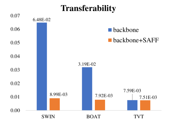
Figure 4: The transferability comparison: average inter-domain distance ${D_{s\leftrightarrow t}}$ of different backbone and backbone + SAFF on VisDA-2017 dataset, where smaller distance indicates better transferability.

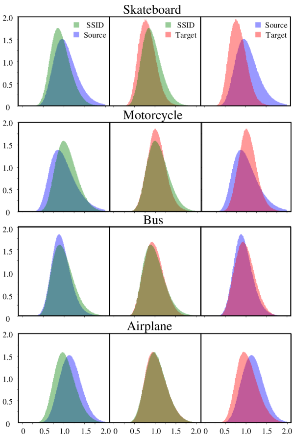
Figure 5: Pairwise distance distribution for four categories randomly selected from the twelve categories of VisDA-2017 dataset. The blue, green, and orange histograms represent the distribution of source domain, SSID, and target domain, respectively.

Meanwhile, as shown in Fig. 5, we randomly select four categories in the VisDA-2017 dataset and draw the pair-wise distance histograms according to the Johnson-Lindenstrauss theorem. The blue, green, and red histograms represent the feature distributions of the source domain, SSID, and target domain, respectively. As a whole, it can be seen that the feature distribution difference between the source domain and the target domain is the largest, and the difficulty of direct transfer is relatively high. The feature distribution difference between source domain $\&$ SSID and target domain $\&$ SSID is relatively small, indicating that SSID is able to transfer the distribution of the source to the target domain, which has successfully improved the transferability between domains.

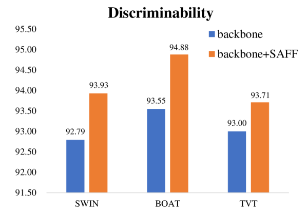
Figure 6: The discriminability comparison: accuracy of all samples in the source and target domains of different backbone and backbone + SAFF on VisDA-2017 dataset, where higher accuracy means better discriminability.

To further demonstrate the improvement of the proposed SAFF in discriminability, the average accuracy of all samples in the source and target domains of VisDA-2017 dataset is calculated to verify how well the class-discriminative information is preserved during the transfer process, as shown in Fig. 6. Obviously, the proposed SAFF performs better, with the overall classification accuracy of SWIN+SAFF, BOAT+SAFF, and TVT+SAFF improving by 1.16$\%$, 0.88$\%$ and 1.11$\%$ over the SWIN, BOAT and TVT backbones, respectively. It can be concluded that SAFF is able to retain more class-discriminative information and thus improve discriminability.

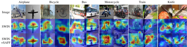
Figure 7: Grad-CAM visualizations on VisDA-2017 dataset. “Image” rows present the random original images from the dataset, ”SWIN” and “SWIN+SAFF” rows present the results of the Grad-CAM visualization obtained by SWIN and SWIN+SAFF respectively. Column Airplanes, Bicycles, Bus, etc. provide the image of corresponding categories in the dataset. The network tends to focus more on the red region and less on the blue-violet region.

In addition, we further compare the Grad-CAM visualizations [68] of SWIN and SWIN+SAFF in each class on VisDA-2017 dataset and randomly select six classes for presentation, as shown in Fig. 7. In the figure, red represents areas with high network attention, and blue-violet represents areas with low attention. As shown, SWIN+SAFF pays more attention to the discriminative features of objects, which further illustrates that SAFF can improve the discriminability of the network. Specifically, the attention of SWIN+SAFF is mainly focused on the backbone skeleton that can reflect the object category, such as the head and wing of an airplane, the two tires, and frame of a bicycle, the body of a train, and the blade of a knife, etc. In contrast, the focus of SWIN is shifted to a certain extent, such as the head of an airplane, a tire or frame of a bicycle, a small part of the body of a train, and food around a knife. Therefore, it is easier for SWIN+SAFF to infer the correct class of objects based on regions of interest. Furthermore, when more than one class of objects is present in the sample, SWIN+SAFF can better focus on the correct class with less effect of distractors. For example, in bus and motorcycle identification, SWIN focuses most of the attention on the surrounding vehicles and cyclists, while SWIN+SAFF focuses on the main body of the bus and the motorcycle, almost paying no attention to surrounding objects. Therefore, these visualization results further demonstrate that the proposed SAFF can improve the discriminability of the network.

5 CONCLUSION

Focusing on the challenges in UDA, we proposed a novel SAFF to bridge the large domain gap and transfer knowledge while alleviating the loss of class-discriminative information with negligible computational costs. It is the first time to introduce the SSID and its corresponding learning strategy to obtain labeled and style-rich features for knowledge transfer. Also, we designed a novel memory bank and intra-/inter-domain loss, and validate their effectiveness in improving transferability and discriminability, while demonstrating for the first time the convergence of the loss function in the latent feature space simulated by infinite sampling through mathematical theory. Finally, the proposed SAFF was applied to various UDA backbones and can yield significant improvements. Comprehensive experimental results on two challenging cross-domain datasets have demonstrated the efficacy and generality of our proposed SAFF.

References

- [1] K. He, X. Zhang, S. Ren, and J. Sun, “Deep residual learning for image recognition,” In IEEE Conference on Computer Vision and Pattern Recognition, 2016, pp. 770–778.
- [2] G. Huang, Z. Liu, L. V. D. Maaten, and K. Q. Weinberger, “Densely connected convolutional networks,” In IEEE Conference on Computer Vision and Pattern Recognition, 2017, pp. 4700–4708.
- [3] S. Minaee, et al, “Image segmentation using deep learning: A survey,” In IEEE Transactions on Pattern Analysis and Machine Intelligence, 2021.
- [4] S. Qi, et al, “Review of multi-view 3D object recognition methods based on deep learning,” Displays, vol. 69, pp. 102053, 2021.
- [5] M. Wang, and W. Deng, “Deep visual domain adaptation: A survey,” Neurocomputing, vol. 312, pp. 135-153, 2018.
- [6] M. Long, Yue Cao, J. Wang, and M. I. Jordan, “Learning transferable features with deep adaptation networks,” In International Conference on Machine Learning, 2015, pp. 97-105.
- [7] M. Long, H. Zhu, J. Wang, and M. I. Jordan, “Deep transfer learning with joint adaptation networks,” In International Conference on Machine Learning. PMLR, 2017, pp. 2208-2217.
- [8] B. Sun, J. Feng, and K. Saenko, “Correlation alignment for unsupervised domain adaptation,” In Domain Adaptation in Computer Vision Applications. Springer, 2017, pp. 153-171.
- [9] J. Zhuo, S. Wang, W. Zhang, and Q. Huang, “Deep unsupervised convolutional domain adaptation,” In Proceedings of the 25th ACM International Conference on Multimedia, 2017, pp. 261-269
- [10] N. Courty, R. Flamary, D. Tuia, and A. Rakotomamonjy, “Optimal transport for domain adaptation,” IEEE Transactions on Pattern Analysis and Machine Intelligence, vol. 39, no. 9, pp. 1853-1865, 2016.
- [11] B. B. Damodaran, B. Kellenberger, R. Flamary, D. Tuia, and N. Courty, “Deepjdot: Deep joint distribution optimal transport for unsupervised domain adaptation,” In Proceedings of the European Conference on Computer Vision (ECCV), 2018, pp. 4470463.
- [12] M. Li, Y. M. Zhai, Y. W. Luo, P. F. Ge, and C. X. Ren, “Enhanced transport distance for unsupervised domain adaptation,” In Proceedings of the IEEE/CVF Conference on Computer Vision and Pattern Recognition, 2020, pp. 13936-13944.
- [13] Z. Zhang, M. Wang, and A. Nehorai, “Optimal transport in reproducing kernel hilbert spaces: Theory and applications,” IEEE Transactions on Pattern Analysis and Machine Intelligence, vol. 42, no. 7, pp. 1741-1754, 2020.
- [14] K. Saito, D. Kim, S. Sclaroff, T. Darrell, and K. Saenko, “Semi-supervised domain adaptation via minimax entropy,” In Proceedings of the IEEE/CVF International Conference on Computer Vision, 2019, pp. 8050-8058.
- [15] S. Cui, S. Wang, J. Zhuo, L. Li, Q. Huang, and Q. Tian, “Towards discriminability and diversity: Batch nuclear-norm maximization under label insufficient situations,” In Proceedings of the IEEE/CVF Conference on Computer Vision and Pattern Recognition, 2020, pp. 3941–3950.
- [16] Y. Ganin and V. S. Lempitsky, “Unsupervised domain adaptation by backpropagation,” In International Conference on Machine Learning, PMLR, 2015, pp. 1180-1189.
- [17] M. Long, Z. Cao, J. Wang, and M. I. Jordan, “Conditional adversarial domain adaptation,” Advances in Neural Information Processing Systems, pp. 31, 2018.
- [18] X. Chen, S. Wang, M. Long, and J. Wang, “Transferability vs. Discriminability: Batch Spectral Penalization for Adversarial Domain Adaptation,” In International Conference on Machine Learning, 2019, pp. 1081–1090.
- [19] K. Saito, K. Watanabe, Y. Ushiku, and T. Harada, “Maximum classifier discrepancy for unsupervised domain adaptation,” In Maximum Classifier Discrepancy for Unsupervised Domain Adaptation, 2018, pp. 3723-3732.
- [20] J. Liang, D. Hu, and J. Feng, “Domain adaptation with auxiliary target domain-oriented classifier,” In IEEE Conference on Computer Vision and Pattern Recognition, 2021, pp. 16632–16642.
- [21] P. E. Bryant and T. Trabasso, “Transitive inferences and memory in young children,” Nature, 1971.
- [22] J. Liang, R. He, Z. Sun, and T. Tan, “Aggregating randomized clustering-promoting invariant projections for domain adaptation,” IEEE Transactions on Pattern Analysis and Machine Intelligence, vol. 41, no. 5, pp. 1027–1042, 2018.
- [23] Y. Chen, W. Li, C. Sakaridis, D. Dai, and L. V. Gool, “Domain adaptive faster r-cnn for object detection in the wild,” In IEEE Conference on Computer Vision and Pattern Recognition, 2018.
- [24] Y.-H. Tsai, W.-C. Hung, S. Schulter, K. Sohn, M.-H. Yang, and M. Chandraker, “Learning to adapt structured output space for semantic segmentation,” In IEEE Conference on Computer Vision and Pattern Recognition, 2018.
- [25] X. Glorot, A. Bordes, and Y. Bengio, “Domain adaptation for large-scale sentiment classification: a deep learning approach,” In International Conference on Machine Learning, 2011.
- [26] K. Mei, C. Zhu, J. Zou, and S. Zhan, “Instance adaptive self-training for unsupervised domain adaptation,” In European Conference on Computer Vision, Springer, Cham, 2020, pp. 415-430.
- [27] Y. Zou, Z. Yu, B. Kumar, and J. Wang, “Unsupervised domain adaptation for semantic segmentation via class-balanced self-training,” In European Conference on Computer Vision, 2018, pp. 289-305.
- [28] Y. Zou, Z. Yu, X. Liu, B. Kumar, and J. Wang, “Confidence regularized self-training,” In Proceedings of the IEEE/CVF International Conference on Computer Vision, 2019, pp. 5982-5991.
- [29] M. Xie, et al, “Learning Distinctive Margin toward Active Domain Adaptation,” In Proceedings of the IEEE/CVF Conference on Computer Vision and Pattern Recognition, 2022, pp. 7993-8002.
- [30] B. Gong, Y. Shi, F. Sha, and K. Grauman, “Geodesic flow kernel for unsupervised domain adaptation,” In Proceedings of the IEEE/CVF Conference on Computer Vision and Pattern Recognition, 2012, pp. 2066-2073.
- [31] R. Gopalan, R. Li, and R. Chellappa, “Unsupervised adaptation across domain shifts by generating intermediate data representations,” IEEE Transactions on Pattern Analysis and Machine Intelligence, vol. 36, no. 11, 2013.
- [32] Y. Dai, J. Liu, Y. Sun, Z. Tong, C. Zhang, L. Y. Duan, “Idm: An intermediate domain module for domain adaptive person re-id,” In Proceedings of the IEEE/CVF International Conference on Computer Vision, 2021, pp. 11864-11874.
- [33] Y. Sun, et al, “A GAN-based domain adaptation method for glaucoma diagnosis,” In International Joint Conference on Neural Networks, 2020.
- [34] S. Li, et al, “Transferable semantic augmentation for domain adaptatio,” In Proceedings of the IEEE/CVF Conference on Computer Vision and Pattern Recognition, 2021.
- [35] T. Xu, W. Chen, P. Wang, F. Wang, H. Li, and R. Jin, “Cdtrans: Cross-domain transformer for unsupervised domain adaptation,” arXiv preprint arXiv:2201.13027, 2022.
- [36] G. Yang, et al, “Transformer-based source-free domain adaptation,” arXiv preprint arXiv:2105.14138, 2021.
- [37] J. Yang, J. Liu, N. Xu, and J. Huang, “Tvt: Transferable vision transformer for unsupervised domain adaptation,” arXiv preprint arXiv:2108.05988, 2021.
- [38] A. Dosovitskiy, et al, “An image is worth 16x16 words: Transformers for image recognition at scale,” In International Conference on Learning Representations, 2021.
- [39] S. Khan, et al, “Transformers in vision: A survey,” ACM Computing Surveys (CSUR), 2021.
- [40] X. Li, Y. Hou, P. Wang, Z. Gao, M. Xu, and W. Li, “Trear: Transformer-based rgb-d egocentric action recognition,” IEEE Transactions on Cognitive and Developmental Systems, vol. 14, no. 1, pp. 246-252, 2021.
- [41] Y. H. H. Tsai, Shaojie Bai, P. P. Liang, J. Z. Kolter, L. P. Morency, and R. Salakhutdinov, “Multimodal transformer for unaligned multimodal language sequences,” Proceedings of the Conference. Association for Computational Linguistics. Meeting. NIH Public Access, 2019, pp. 6558.
- [42] X. Huang and S. Belongie, “Arbitrary style transfer in real-time with adaptive instance normalization,” In Proceedings of the IEEE International Conference on Computer Vision, 2017, pp. 1501-1510.
- [43] D. Ulyanov, A. Vedaldi, and V. Lempitsky, “Improved texture networks: Maximizing quality and diversity in feed-forward stylization and texture synthesis,” In Proceedings of the IEEE Conference on Computer Vision and Pattern Recognition, 2017, pp. 6924-6932.
- [44] D. Vincent, S. Jonathon and K. Manjunath, “A learned representation for artistic style,” arXiv preprint arXiv:1610.07629, 2016.
- [45] X. Peng, B. Usman, N. Kaushik, J. Hoffman, D. Wang, and K. Saenko, “Visda: The visual domain adaptation challenge,” arXiv preprint arXiv:1710.06924, 2017.
- [46] H. Venkateswara, J. Eusebio, S. Chakraborty, and S. Panchanathan, “Deep hashing network for unsupervised domain adaptation,” In Proceedings of the IEEE Conference on Computer Vision and Pattern Recognition, 2017, pp. 5018–5027.
- [47] Z. Liu, et al, “Swin transformer: Hierarchical vision transformer using shifted windows,” In Proceedings of the IEEE/CVF International Conference on Computer Vision, 2021.
- [48] Y. Tan, et al, “BOAT: Bilateral Local Attention Vision Transformer,” arXiv preprint arXiv:2201.13027, 2022.
- [49] P. O. Pinheiro, “Unsupervised domain adaptation with similarity learning,” In Proceedings of the IEEE Conference on Computer Vision and Pattern Recognition, 2018, pp. 8004-8013.
- [50] Y. Wu, D. Inkpen, and A. El-Roby, “Dual mixup regularized learning for adversarial domain adaptation,” In European Conference on Computer Vision, Springer, Cham, 2020, pp. 540-555.
- [51] M. Xu, et al, “Adversarial domain adaptation with domain mixup,” In Proceedings of the AAAI Conference on Artificial Intelligence, 2020, vol. 34, no. 04, pp. 6502-6509.
- [52] C. Y. Lee, T. Batra, M. H. Baig, and D. Ulbricht, “Sliced Wasserstein discrepancy for unsupervised domain adaptation,” In Proceedings of the IEEE/CVF Conference on Computer Vision and Pattern Recognition, 2019, pp. 10285-10295.
- [53] Y. Pan, T. Yao, Y. Li, Y. Wang, C.-W. Ngo, and T. Mei, “Transferrable prototypical networks for unsupervised domain adaptation,” In Proceedings of the IEEE/CVF Conference on Computer Vision and Pattern Recognition, 2019.
- [54] W.-G. Chang, T. You, S. Seo, S. Kwak, and B. Han, “Domain-specific batch normalization for unsupervised domain adaptation,” In Proceedings of the IEEE/CVF Conference on Computer Vision and Pattern Recognition, 2019.
- [55] Z. Du, J. Li, H. Su, L. Zhu, and K. Lu, “Cross-domain gradient discrepancy minimization for unsupervised domain adaptation,” In Proceedings of the IEEE/CVF Conference on Computer Vision and Pattern Recognition, 2021.
- [56] H. Liu, et al, ”Transferable adversarial training: A general approach to adapting deep classifiers”, In International Conference on Machine Learning, PMLR, 2019, pp.4013-4022.
- [57] H. Touvron, M. Cord, M. Douze, F. Massa, A. Sablayrolles, and H. Jegou, “Training data-efficient image transformers distillation through attention,” In International Conference on Machine Learning. PMLR, 2021, pp. 10347-10357.
- [58] S. Cui, S.i Wang, J. Zhuo, C. Su, Q. Huang, and Q. Tian, ”Gradually vanishing bridge for adversarial domain adaptation,” In Proceedings of the IEEE/CVF Conference on Computer Vision and Pattern Recognition, 2020, pp. 12455–12464.
- [59] Y. Liu, et al, “Unsupervised Domain Adaptation by Optimal Transportation of Clusters Between Domains,” [Online]. Available: https://openreview.net/pdf?id=q5ru7alcpfM
- [60] J. Liang, D. Hu, and J. Feng, “Do we really need to access the source data? Source hypothesis transfer for unsupervised domain adaptation,” In International Conference on Machine Learning. PMLR, 2020.
- [61] Q. Zeng, T. Luo, and B. Wang, “Domain-Augmented Domain Adaptation,” arXiv preprint arXiv:2202.10000, 2022.
- [62] S. Zhang, T. Lin, and Y. Xu, “Boosting Unsupervised Domain Adaptation with Soft Pseudo-label and Curriculum Learning,” arXiv preprint arXiv:2112.01948, 2021.
- [63] J. Liang, D. Hu, and J. Feng, “Domain adaptation with auxiliary target domain-oriented classifier,” In Proceedings of the IEEE/CVF Conference on Computer Vision and Pattern Recognition, 2021, pp. 16632-16642.
- [64] L. Chen, et al, “Reusing the Task-specific Classifier as a Discriminator: Discriminator-free Adversarial Domain Adaptation,” In Proceedings of the IEEE/CVF Conference on Computer Vision and Pattern Recognition, 2022, pp. 7181-7190.
- [65] N. Ding, et al, “Source-Free Domain Adaptation via Distribution Estimation,” In Proceedings of the IEEE/CVF Conference on Computer Vision and Pattern Recognition, 2022, pp. 7212-7222.
- [66] B. Xie, et al, “Active Learning for Domain Adaptation: An Energy-based Approach,” arXiv preprint arXiv:2112.01406, 2021.
- [67] W. Ma, et al, “Exploiting Both Domain-specific and Invariant Knowledge via a Win-win Transformer for Unsupervised Domain Adaptation,” arXiv preprint arXiv:12941, 2021.
- [68] R. R. Selvaraju, et al, “Grad-cam: Visual explanations from deep networks via gradient-based localization,” In Proceedings of the IEEE international conference on computer vision, 2017, pp. 618-626.
Acknowledgment
This work was supported by the National Natural Science Foundation of China (Nos. 62136004, 61732006, 61876082).